Summary The Washington Legislature directed the Washington State Institute for Public Policy to begin conducting economic analyses of certain K–12 policies. Augmenting the work of the recent Washington Learns process, this report describes our initial cost-benefit findings for class size reductions and full-day vs. half-day kindergarten. Upcoming reports will examine other K–12 topics.

Research Approach We examine all rigorous research studies to estimate whether academic achievement can be expected to improve with each policy. We also compute an expected return on investment by estimating long-run labor market and other non-market benefits of improved academic outcomes.

Finding: Class Size Reductions We analyze 38 recent high-quality evaluations of whether reducing the number of students in a classroom improves student test scores. The results are mixed. We find that during kindergarten through second grade, there is evidence that reducing class size increases test scores. During third through sixth grade, the gains remain significant but are much smaller—only 35 percent of the kindergarten through second grade gains. In middle and high school, we find that reduced class sizes do not lead to statistically significant test score gains. We estimate that reductions in class size in kindergarten through second grade produce a 6 to 11 percent annual real rate of return on investment.

Finding: Full-Day vs. Half-Day Kindergarten We analyze 23 rigorous evaluations and find that full-day kindergarten, compared with half-day kindergarten, produces a statistically significant boost to test scores during, or shortly after, kindergarten. These positive early gains, however, appear to erode almost completely during grades one through three. Thus, for full-day kindergarten to generate long-term academic benefits, public policies need to examine how to sustain the early gains from any investments in full-day kindergarten. Experimentation seems warranted.

‡ Suggested citation: Steve Aos, Marna Miller, & Jim Mayfield. (2007). Benefits and Costs of K–12 Educational Policies: Evidence-Based Effects of Class Size Reductions and Full-Day Kindergarten. Olympia: Washington State Institute for Public Policy, Document No. 07-03-2201. Contact email: saos@wsipp.wa.gov.

Initial Report March 2007

BENEFITS AND COSTS OF K–12 EDUCATIONAL POLICIES: Evidence-Based Effects of Class Size Reductions and Full-Day Kindergarten‡

The Washington State Legislature directed the Washington State Institute for Public Policy (Institute) “to begin the development of a repository of research and evaluations of the cost-benefits of various K–12 educational programs and services.”1 This report contains our initial findings on two topics: class size reductions and full-day kindergarten. We examine existing research evidence to estimate whether student academic achievement can be expected to improve with each policy. We also compute the expected return on investment for the two options. Upcoming reports will include other K–12 topics. This research assignment from the Legislature is designed to augment the recent Washington Learns process—the statewide effort to identify ways to improve Washington’s early learning, K–12, and higher education systems. In its final report issued in November 2006, the Washington Learns Steering Committee adopted principles for changing Washington’s public education system. Among other recommendations, the Committee stated that Washington “will invest only in programs that work” and that the state “must be diligent about redirecting current educational dollars into proven strategies for improved results.”2 Following these principles, the purpose of this research is to estimate the likely costs and benefits of “research-proven” K–12 policies and programs. Any attempt to calculate costs and benefits encounters a high analytical bar. Conducting this type of study implies being able to answer central questions about causality. That is, if costs are incurred, will benefits be obtained?

Washington State Institute for Public Policy

110 Fifth Avenue Southeast, Suite 214 • PO Box 40999 • Olympia, WA 98504-0999 • (360) 586-2677 • FAX (360) 586-2793 • www.wsipp.wa.gov

Continues on page 2

2

These questions are, of course, difficult to answer because in the real world few things can be known with certainty. Determining causality, however, is not a problem unique to education policy. Almost all business and public policy decisions involve different degrees of risk and uncertainty in knowing whether desired outcomes can be secured with a given strategy. In this report, we describe the steps we have taken to identify whether the costs of certain evidence-based K–12 policies and programs are likely to relate to student outcomes. Our analytical work is not yet complete; rather, this is our first report describing progress to date. Comments are welcomed. For this current assignment on K–12 topics, the Institute is building on its previous analyses of the costs and benefits of other public policies. The Washington State legislature has, in recent years, directed the Institute to examine evidence-based programs related to prevention, early intervention, mental health, substance abuse treatment, and criminal justice policies for both juveniles and adults.3 In these previous studies, the legislature also asked the Institute to estimate the costs and benefits of research-based approaches. This report begins by describing, briefly, our research approach. We then present and discuss our findings for the two K–12 topics covered in this report: class size reductions and full-day kindergarten. For readers interested in technical matters, we also include an appendix, beginning on page 16, that provides greater detail on the Institute’s analytic procedures, economic methods, and results. Research Approach In this initial review of K–12 topics, we focus on a single type of educational outcome: student academic performance. In addition to academic skills, of course, public expectations place many other goals on the K–12 system. These additional goals include improved non-cognitive outcomes such as promoting individual discipline and a work ethic, citizenship, reduced criminal activity, reduced drug and alcohol abuse, reduced teen pregnancy, and so on.4 While these goals are important, our initial review focuses on a narrower question: What works to improve academic outcomes? This outcome is especially timely, because state and federal polices have placed student academic performance as the prime outcome measure for the K–12 system.

The types of academic outcomes that we analyze depend on the specific measures used in the existing K–12 evaluation studies we review. These academic outcome measures include, but are not limited to, the following:

Standardized test scores;

Course grades or grade point averages;

Grade retention;

Years in special education;

High school graduation/dropping out; and

Longer-range outcomes such as college attendance, college graduation, employment, and earnings.

Our research approach involves two general steps. Step One: What Works? What Doesn’t? In order to estimate whether a particular type of K–12 program or policy is likely to affect student academic performance, we systematically assess the findings of all methodologically sound research studies we can locate. For each high-quality evaluation we find, we compute an “effect size”—a

Legislative Study Direction

The 2006 Washington State Legislature directed the Institute to initiate research that will provide Washington with an on-going analysis of evidence-based K–12 programs and services, as well as cost-benefit analyses of each approach. The language initiating the study was in Engrossed Substitute Senate Bill 6386 §607 (15) which directed the Institute to:

“…begin the development of a repository of research and evaluations of the cost-benefits of various K–12 educational programs and services. The goal for the effort is to provide policymakers with additional information to aid in decision making. Further, the legislative intent for this effort is not to duplicate current studies, research, and evaluations but rather to augment those activities on an on-going basis. Therefore, to the extent appropriate, the institute shall utilize and incorporate information from the Washington learns study, the joint legislative audit and review committee, and other entities currently reviewing certain aspects of K–12 finance and programs. The institute shall provide the following: (a) By September 1, 2006, a detailed implementation plan for this project; (b) by March 1, 2007, a report with preliminary findings; and (c) annual updates each year thereafter.”

3

statistical summary measure indicating the degree to which an evaluated policy or program changes an academic outcome. Then, for a group of studies on a particular K–12 topic, we combine the effect sizes to determine whether, on average, outcomes can be expected to change with the program or policy under consideration.5 While it may be tempting to examine only one or two studies on a topic, we think a restricted review of existing research may lead to unrealistic or biased expectations. By considering all methodologically sound studies on a topic, our approach seeks to determine the average evidence-based effectiveness of each K–12 topic. One always hopes for above-average performance—a so called “Lake Wobegon” effect—but for the K–12 taxpayer investments considered in this review, we think it is more prudent to base expectations on the average evidence-based result. An analogy may help explain our approach: investing in the stock market. If one is interested in knowing the likely return from investing in the stock market, it is better to examine the historical and expected returns of many stocks rather than focusing on one stock that has performed exceptionally well. Thus, a broad stock market index like the S&P 500 provides a more realistic gauge of expected stock market returns than the historical return of any one exceptional stock, such as Microsoft. One always hopes for a Microsoft-like return, but expectations are more likely to be fulfilled by anticipating the average performance of many stocks. Following this logic, for example, if one wants to know whether a typical real-world investment in preschool improves the academic outcomes for low-income children, it is more prudent to assess the results of all methodologically sound studies that have been done on preschools for this population (the equivalent of the S&P 500 approach) rather than selecting one preschool study that happened to achieve exceptional returns (the Microsoft analogy). Unless one has inside knowledge of how to pick consistently the next Microsoft, or confidence that schools can duplicate regularly the all-time best preschool approach, then it is safer to assume an average return based on a larger group of results. Thus, our approach to determining “What Works?” is to review all of the methodologically sound studies on a topic in order to estimate the likely return on investment for a typical, real-world, K–12 program or policy.

We include studies in our review after screening for methodological rigor and relevance for Washington State. We include random assignment studies, although there are relatively few of these “gold-standard” studies. Therefore, we also include rigorous quasi-experimental or observational studies when special methodological care has been taken to isolate the causal effect of a K–12 policy or program on academic outcomes. In the education field, paying close attention to a study’s methodological quality appears to be especially important because parents, students, schools, and voters each exert a considerable influence on how students and educational resources are distributed. This real-world non-random sorting of students and resources can make it difficult for a study to isolate the causal effect of a program or policy on student outcomes. A study with very good data can statistically control for some or perhaps many of these factors, but usually there are other factors—unobserved to the researcher—that can confound the ability of a study to identify causal effects. Fortunately, as we discuss, there have been recent advances in datasets, as well as increased use of advanced statistical methods, that have allowed researchers to improve their ability to identify important outcomes of certain education policies and programs. Step Two: What Are the Expected Returns on Investment? One of the precepts of economics is that “there is no such thing as a free lunch.” Each of the programs and policies discussed in this report can cost taxpayers money. Therefore, in addition to estimating whether research indicates something works, it is also important to estimate whether the benefits of an approach outweigh its costs. In this study, we conduct an economic analysis by stacking the expected monetary value of any statistically significant benefits against the costs of the program or policy. To do this, we have developed, and are continuing to refine, techniques to measure costs and benefits associated with the outcomes of K–12 programs, policies, and services. We use the findings from recent economic research to provide a range of estimates of the benefits of statistically significant educational outcomes. We model these outcomes in a “human capital” framework. Economists such as Alan Krueger and Eric Hanushek, who often disagree on whether certain K–12 policies achieve outcomes, generally use a similar human capital approach to monetize the benefits of any outcomes obtained.6 In the

4

human capital model, successful investments in K–12 policies and programs (i.e., investments that have an evidence-based ability to boost academic performance), are estimated to generate benefits over a number of years into the future. The benefits typically include labor market and other types of non-market benefits. We summarize these monetary costs and benefits with the usual set of financial summary statistics: net present values, benefit-to-cost ratios, and rates of return on investment. As in our previous cost-benefit analyses, we estimate life-cycle costs and benefits from two perspectives: first, we estimate the benefits that accrue directly to program participants (in this case, the students), and second, we estimate the benefits that accrue to non-participants. For example, a student who scores higher on standardized tests can be expected to enjoy the benefit of greater earnings in the labor market compared with students who do not score as well.7 Non-participants benefit from the taxes paid on those increased earnings. Economists have also been examining whether improved K–12 outcomes are related to other desirable outcomes such as: reduced crime; improved health care and lower health care costs; reduced foster care; so-called “knowledge spillovers” that stimulate general economic growth; and increased civic participation.8 While the research underlying many of these non-market outcomes is more uncertain and less well developed than the labor market outcomes, we conduct sensitivity analyses to test how the range of total benefits might be affected by successful K–12 educational policies. The appendix to this report describes our economic procedures in detail.

K–12 Topics Scheduled for Evidence-Based

Reviews and Cost-Benefit Analyses

The assignment from the Legislature was “to begin the development of a repository of research and evaluations of the cost-benefits of various K–12 programs and services.” In addition to the two topics covered in this initial report, we have also begun work on a number of additional topics by collecting and analyzing the relevant research literature. The work on several of these additional topics is underway but not yet complete; results will be presented in upcoming reports.

Topics for upcoming reports include, but are not limited to the following:

Preschool education

Dropout prevention programs

Professional development activities

Effect of school size

Teacher quality effects

Alternative education programs

English language learner programs

Charter schools

Vouchers

Other early learning approaches

Teacher aides

Mentors for students

Mentors for new teachers

Tutoring

Teacher compensation

Summer school

Extended day/weekend programs

Grade retention

5

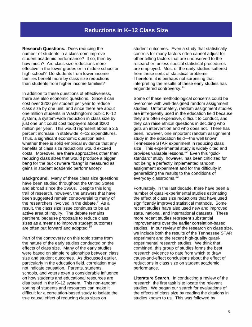
Research Questions. Does reducing the number of students in a classroom improve student academic performance? If so, then by how much? Are class size reductions more effective in the lower grades or in middle school or high school? Do students from lower income families benefit more by class size reductions than students from higher income families? In addition to these questions of effectiveness, there are also economic questions. Since it can cost over $200 per student per year to reduce class size by one unit, and since there are about one million students in Washington’s public K–12 system, a system-wide reduction in class size by just one unit could cost taxpayers about $200 million per year. This would represent about a 2.5 percent increase in statewide K–12 expenditures. Thus, a significant economic question asks whether there is solid empirical evidence that any benefits of class size reductions would exceed costs. Moreover, are there approaches other than reducing class sizes that would produce a bigger bang for the buck (where “bang” is measured as gains in student academic performance)? Background. Many of these class size questions have been studied throughout the United States and abroad since the 1960s. Despite this long trail of research, however, the answers that have been suggested remain controversial to many of the researchers involved in the debate.9 As a result, the class size issue continues to be an active area of inquiry. The debate remains pertinent, because proposals to reduce class sizes as a means to improve student outcomes are often put forward and adopted.10 Part of the controversy on this topic stems from the nature of the early studies conducted on the effects of class size. Many of the early studies were based on simple relationships between class size and student outcomes. As discussed earlier, particularly in the education field, correlation may not indicate causation. Parents, students, schools, and voters exert a considerable influence on how students and educational resources are distributed in the K–12 system. This non-random sorting of students and resources can make it difficult for a correlation-based study to isolate the true causal effect of reducing class sizes on

student outcomes. Even a study that statistically controls for many factors often cannot adjust for other telling factors that are unobserved to the researcher, unless special statistical procedures are employed. Most of the early studies suffered from these sorts of statistical problems. Therefore, it is perhaps not surprising that interpreting the results of these early studies has engendered controversy.11 Some of these methodological concerns could be overcome with well-designed random assignment studies. Unfortunately, random assignment studies are infrequently used in the education field because they are often expensive, difficult to conduct, and they can raise ethical questions in deciding who gets an intervention and who does not. There has been, however, one important random assignment study in the education field—the well known Tennessee STAR experiment in reducing class size. This experimental study is widely cited and provides valuable lessons.12 Even this “gold-standard” study, however, has been criticized for not being a perfectly implemented random assignment experiment and for the difficulty in generalizing the results to the conditions of everyday classrooms.13 Fortunately, in the last decade, there have been a number of quasi-experimental studies estimating the effect of class size reductions that have used significantly improved statistical methods. Some recent studies have also used new and improved state, national, and international datasets. These more recent studies represent substantial improvements over the earlier correlation-based studies. In our review of the research on class size, we include both the results of the Tennessee STAR experiment and the recent high-quality quasi-experimental research studies. We think that, combined, this group of studies forms the best research evidence to date from which to draw cause-and-effect conclusions about the effect of reductions in class size on student academic performance. Literature Search. In conducting a review of the research, the first task is to locate the relevant studies. We began our search for evaluations of the effects of class size by reading the citations in studies known to us. This was followed by

Reductions in K–12 Class Size

6

searching the internet and academic library information systems for published or yet-to-be published studies. We then read and screened all prospective studies for methodological rigor and relevance for Washington State policy questions. Individual authors of the studies frequently needed to be contacted to obtain additional information. We found 38 class size studies with sufficient methodological rigor to include in our analysis. The citations to these studies are listed in Exhibit 5. Characteristics of the Studies Included in Our Review. Exhibit 1 lists some of the characteristics of the 38 methodologically sound studies included in our review. The majority of the studies were written or published recently. The oldest study was published in 1989, seven were published between 1995 and 1999, and 30 were published from 2000 to 2006.

Exhibit 1 Description of Studies Included

Number Pct. Number of studies included in analysis 38 100% Publication Date 1980s 1 3% 1995 to 1999 7 18% 2000 to 2006 30 79%

Number of grade-level effect sizes (ES) 69

Domestic or International grade-level ES United States 34 49% International 35 51%

Methodology of grade-level ES Instrumental variables (IV) or regression discontinuity design 43 62%

Hierarchical linear model or ordinary least squares regression 14 20%

Fixed effects regression without an IV 4 6% Random assignment 8 12%

Outcome variable: student test scores 67 97% Outcome variable: other (graduation) 2 3% Policy variable: class size change 62 90% Policy variable: K–12 spending 7 10%

Grade when the resources were spent to lower class size

Kindergarten through third grade 18 26% Fourth through sixth grade 25 36% Seventh through eighth grade 18 26% Ninth through twelfth grade 8 12% These studies contributed 69 separate tests of whether reductions in K–12 class sizes affect student academic performance. The reason there are more tests than studies is that some studies estimated results of class size reductions for different grade levels. In our analysis, the unit of observation is the estimated effect size for a one-

unit change in class size for the grade level in which the resources were spent. About 49 percent of the separate tests were from studies conducted in the United States and the remaining were of populations outside the United States. We excluded international studies where class sizes are at substantially different levels than those found in the United States. As we describe, we also tested to determine whether results from United States class size studies are significantly different from international studies. In terms of methodology, about 62 percent of these effects were from studies that employed an instrumental variables or regression discontinuity design; 20 percent used a correlation-based design (a hierarchical linear model or ordinary least squares) with rich datasets that allowed the researchers to include a considerable number of statistical controls; about 6 percent used a fixed effects panel data approach without an instrumental variable; and there were two random assignment studies. For the Tennessee STAR study, we included two reports that independently analyzed the data from this important study.14 Of these 69 separate tests, 97 percent directly measured whether standardized test scores were influenced by changes in class size, and about 3 percent measured whether high school graduation rates were influenced by class size changes. We also examined studies testing whether changes in K–12 spending influenced standardized test scores; seven of the 69 separate tests (10 percent) in our analyses were of this form. Even though this last group of studies does not measure class size directly, we included their findings because a high proportion of K–12 operational spending is for teaching staff and, therefore, expenditures are probably a reasonable proxy for changes in class size. We did, however, conduct our overall analysis with and without this last group of studies included. Twenty-six percent of the 69 tests were for class size reductions primarily in kindergarten through second grade. Thirty-six percent were for reductions in grades three through six, 26 percent occurred during seventh through eighth grades, and 12 percent during high school.

7

Results and Findings. To measure results, we calculate an “effect size” for each of the 69 separate tests contributed by the 38 studies in our review. An effect size is a statistical summary measure describing the degree to which academic performance is improved as a result of a reduction in class size. The bigger the effect size, the bigger the impact. An effect size of zero means there is no effect of the class size reduction on test scores. For technical readers, the appendix describes the procedures we use to calculate effect sizes. An effect size measures the expected change in test scores, expressed in standard deviation units. Washington’s standardized test is the Washington Assessment of Student Learning (WASL). The average student-level score on the 2006 10th-grade math WASL was 401 with a standard deviation of 38. Thus, for example, an educational policy that produces a large effect size of 0.5 would mean an average gain of 19 points on the WASL (19 = .5 X 38), or about a 4.7 percent change in average test scores (.047 = 19 / 401). In our analysis of class size, we calculate the effect of a one-unit change in class size on test scores. For example, our effect sizes measure the change in standard deviation units by moving from a class size of 20 to a class size of 19.15 Exhibit 2 displays a simple plot of the 69 effect sizes arranged by the grade in which the class size reduction took place. Each dot represents an effect size from an individual study and measures the change on average math and/or reading tests. A simple examination of Exhibit 2 indicates that reducing class sizes in kindergarten through the

second grade is consistently associated with positive gains in academic test scores. For third through sixth grade, the results are more mixed with some studies indicating positive results and some indicating lower or negative results. By middle school and high school, the effects appear to be small, on average, and there have been some studies indicating no gain or even a reduced level of academic performance with reduced class sizes. It is also clear that in middle school, the raw results are quite varied, while in high school there are relatively few rigorous studies that have tested the effect of class size reductions. Thus, the simple plot of effect sizes in Exhibit 2 reveals that class size reductions in the early grades are likely to be more effective than during higher grades. We then examine these 69 raw effect sizes with multivariate regression. The purpose of this more in-depth analysis is to refine the simple plot shown in Exhibit 2 by controlling for the characteristics of the studies. As shown in Exhibit 1, some of the studies were from the United States, some were from international locations; some used certain types of statistical identification methodologies, others did not; some used student-level data, others used class- or district-level data. Using standard statistical procedures, we also weight the results of the different studies so that a study that evaluated many students is given more weight than a study that evaluated far fewer students. Our multivariate analyses allow us to test for the significance of these factors. In the appendix we describe our methods and results in technical detail.

Exhibit 2Changes in Academic Achievment

From Reducing Class Size by One Unit

-.04

-.03

-.02

-.01

.00

.01

.02

.03

.04

.05

0 1 2 3 4 5 6 7 8 9 10 11 12Grade in Which the Class Size Was Reduced

K

Each circle is the effect

size from a study, N = 69

Effe

ct S

ize

Gai

ns o

n Av

erag

e M

ath

and

Rea

ding

Tes

ts

8

Our estimated effects from our preferred regression model are presented in Exhibit 3. The findings are consistent with those in Exhibit 2. There are statistically significant effects for two grade levels: kindergarten through second grade, and third through sixth grade, although the effects for the latter group are just 35 percent of the effects for the kindergarten through second grade group. The results for middle and high schools indicate that class size reductions do not generate statistically significant improvements in test scores—note that the 95 percent confidence intervals shown in Exhibit 3 for these two grade level groups include zero as a possibility. Return on Investment (ROI) Calculations. The purpose of this study is to estimate the costs and benefits of K–12 policies and programs. We calculate a return on investment statistic that is computed in the same general way as that for private sector investments. In the appendix, we describe in detail the procedures we use to estimate the monetary benefits associated with the effect sizes we just discussed. We estimate that increased test scores generate monetary benefits beginning at age 18 when the student would begin to be attached to the labor market. We provide a range of returns on investment, since there are several factors that can be estimated only with uncertainty. In particular, we varied these factors (details shown in Exhibit B.2 in the appendix):

1) The estimate of the initial gain is test score effect size, shown in Exhibit 3;

2) An annual rate of decay in this effect size to the end of high school;

3) An average annual real rate of growth in labor market earnings;

4) An estimate of the effect of a gain in test scores on lifetime earnings in the labor market;

5) Alternative social rates of return to account for such non-labor market factors as reduced crime, reduced health care costs, increased civic participation, and “knowledge spillovers” that stimulate general economic growth;

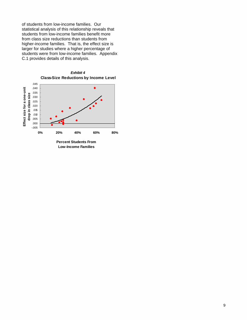
6) Alternative real discount rates. ROI Finding: Class Size Reductions in Kindergarten Through Grade Two. As shown in Exhibit 3, kindergarten through grade two are the grade levels for which we estimate the largest effects on test scores. We estimate that a one-unit drop in class size for these grades would cost about $217 per student per year to pay for the increased operating and capital costs. We estimate that the real internal rate of return on investment for a one-unit drop in class size during kindergarten through second grade ranges from 5.7 to 11 percent. The average return on investment is 8.3 percent.16 Expressed in terms of an average benefit-to-cost ratio, this investment generates $2.79 in benefits for each dollar of cost. For comparison purposes, the long-run annual rate of return on investment for the equities that make up the S&P 500 stock market index is about 4.4 percent per year.17 ROI Finding: Class Size Reductions in Grades Three Through Six. Exhibit 3 indicates that class size reductions in grades three through six generate a significant—but lower—effect on test scores than in the first few grades. This reduced effect means lower returns on investment. We estimate that the real average return on investment for a one-unit drop in class size during grades three through six is about 6 percent, or $1.38 in benefits per dollar of cost. ROI Finding: Class Size Reductions in Middle School and High School. As shown in Exhibit 3, we did not find statistically significant effects for class size reductions in middle and high school, so we did not compute return on investment estimates. Additional Analysis of Low-Income Populations. Some of the studies in our review include information on whether students from low-income families fare better with class size reductions than students from non-low-income families. We conducted an additional analysis for this group of studies, and Exhibit 4 plots effect sizes against the percentage of low-income students reported in these studies. The effect of class size reductions appears greater in classes with larger proportions

Exhibit 3Effect of Class Size Reductions

.019

.007

-.001

.004

-.010

-.005

.000

.005

.010

.015

.020

.025

.030

K to 2 3 to 6 7 to 8 9 to 12

Grade Level When Class Size Reduced

Effe

ct s

ize

for a

one

-uni

t dr

op in

cla

ss s

ize

T he red bo xes are the est imated ef fect

s izes; the vert ical lines are 95%

co nf idence intervals.

9

of students from low-income families. Our statistical analysis of this relationship reveals that students from low-income families benefit more from class size reductions than students from higher-income families. That is, the effect size is larger for studies where a higher percentage of students were from low-income families. Appendix C.1 provides details of this analysis.

Exhibit 4Class-Size Reductions by Income Level

-.005.000.005.010.015.020.025.030.035

.040

.045

0% 20% 40% 60% 80%

Percent Students From Low-Income Families

Effe

ct s

ize

for a

one

-uni

t dr

op in

cla

ss s

ize

10

Exhibit 5 Citations to the Studies Used in the Statistical Analyses of Class Size Reductions

(Some studies contributed independent effect sizes from more than one location or grade level)

Akerhielm, K. (1995). Does class size matter? Economics of Education Review, 14(3): 229-241. Angrist, J. & Lavy, V. (1999). Using Maimonides' Rule to estimate the effect of class size on children's academic achievement. Quarterly Journal of

Economics, 114(2): 533-576. Blatchford, P., Goldstein, H., Martin, C., & Browne, W. (2002). A study of class size effects in English school reception year classes. British Education

Research Journal, 28(2): 169-185. Bonesrønning, H. (2003). Class size effects on student achievement in Norway: Patterns and explanations. Southern Economic Journal, 69(4): 952-965. Borland, M.V., Howsen, R.M., & Trawick, M.W. (2005). An investigation of the effect of class size on student achievement. Education Economics, 13(1):

73-83. Bressoux, P., Kramarz, F., & Prost, C. (2005). Teachers' training, class size and students' outcomes: Evidence from their grade classes in France. Paris,

France: Center for Research in Economics and Statistics. Browning, M. & Heinesen, E. (2005). Class size, teacher hours and educational attainment (CAM Working Papers No. 2003-1). Copenhagen, Denmark:

University of Copenhagen, Department of Economics, Centre for Applied Microeconometrics. Dearden, L., Ferri, J., & Meghir, C. (2002). The effect of school quality on educational attainment and wages. Review of Economics and Statistics, 84(1):

1-20. Dustmann, C., Rajah, N., & van Soest, A. (2003). Class size, education, and wages. The Economic Journal, 113(485): F99-F120. Ecalle, J., Magnan, A., & Gibert, F. (2006). Class size effects on literacy skills and literacy interest in first grade: A large-scale investigation. Journal of

School Psychology, 44(3): 191-209. Feinstein, L. & Symons, J. (1999). Attainment in secondary school. Oxford Economic Papers, 51(2): 300-321. Fergeson, R.F. & Ladd, H.F. (1996). How and why money matters: An analysis of Alabama schools. In H.F. Ladd (Ed.), Holding schools accountable:

Performance-based reform in education (pp. 265-298). Washington: Brookings Institution. Fuchs, T. & Wößmann, L. (2004). What accounts for international difference in student performance? A re-examination using PISA data (Report no.

1287). Bonn, Germany: Institute for the Study of Labor (IZA). Grissmer, D.W. & Flanagan, A. (2006). Improving the achievement of Tennessee students: Analysis of the National Assessment of Educational Progress.

Santa Monica, CA: RAND. Grissmer, D.W., Flanagan, A., Kawata, J., & Williamson, S. (2000). Improving student achievement: What state NAEP test scores tell us. Santa Monica,

CA: RAND. Guryan, J. (2003). Does money matter? Estimates from education finance reform in Massachusetts. Chicago, IL: University of Chicago, Graduate School

of Business. Haegeland, T., Raaum, O., & Salvanes, K.G. (2005). Pupil achievement, school resources and family background (Report No. 1459). Bonn, Germany:

Institute for the Study of Labor (IZA). Hoxby, C.M. (2000). The effects of class size on student achievement: New evidence from population variation. The Quarterly Journal of Economics,

115(4): 1239-1285. Iacovou, M. (2002). Class size in the early years: Is smaller really better? Education Economics, 10(3): 261-290. Jakubowski, M. & Sakowsi, P. (2005). Quasi-experimental estimates of class size effects in primary school in Poland. Warsaw, Poland: Warsaw

University, Faculty of Economics. Jenkins, A., Levacic, R., & Vignoles, A. (2006). Estimating the relationship between school resources and pupil attainment at GCSE (Report No. RR727).

London: University of London, Institute of Education. Jepsen, C. & Rivkin, S. (2002). Class size reduction, teacher quality, and academic achievement in California public elementary schools. San Francisco,

CA: Public Policy Institute of California. Kang, C. (2005). Effects of small classes on academic achievement: Evidence from new entrants to Project STAR. Singapore: National University of

Singapore, Department of Economics. Kinnucan, H.W., Zheng, Y., & Brehmer, G. (2006). State aid and student performance: A supply-demand analysis. Education Economics, 14(4): 487-509. Krueger, A. (1999). Experimental estimates of education production functions. Quarterly Journal of Economics, 114(2): 497-532. Levacic, R., Jenkins, A., Vignoles, A., Steele, F., & Allen, R. (2005). Estimating the relationship between school resources and pupil attainment at Key

Stage 3 (Report No. RR679). London: University of London, Institute of Education. Levin, J. (2001). For whom the reductions count: A quantile regression analysis of class size and peer effects on scholastic achievement. Empirical

Economics, 26(1): 221-246. McGiverin, J., Gilman, D., & Tillitski, C. (1989). A meta-analysis of the relation between class size and achievement. The Elementary School Journal,

90(1): 47-56. Molnar, A., Smith, P., Zahorik, J., Palmer, A., Halbach, A., & Ehrle, K. (1999). Evaluating the SAGE program: A pilot program in targeted pupil-teacher

reduction in Wisconsin. Educational Evaluation and Policy Analysis, 21(2): 165-177. NICHD Early Child Care Research Network. (2004). Does class size in first grade relate to children's academic and social performance or observed

classroom processes? Developmental Psychology, 40(5): 651-664. Papke, L.E. (2006). The effects of changes in Michigan's school finance system. East Lansing, MI: Michigan State University, Department of Economics. Pikkety, T. (2004). Should we reduce class size or school segregation? Theory and evidence from France. Paris, France: ENS-EHESS (as described in

Valdenaire, 2004). Ready, D.D. & Lee, V.E. (2006). Optimal context size in elementary schools: Disentangling the effects of class size and school size. Washington, DC:

Brookings Papers on Education Policy. Rivkin, S.G., Hanushek, E.A., & Kain, J.F. (2005). Teachers, schools, and academic achievement. Econometrica, 73(2): 417. Sander. W. (1999). Endogenous expenditures and student achievement. Economics Letters, 64(2): 223-231. Urquiola, M. (2006). Identifying class size effects in developing countries: Evidence from rural Bolivia. The Review of Economics and Statistics, 88(1): 171-

177. Valdenaire, M. (2006). Do younger pupils need smaller classes? Evidence from France. London: London School of Economics, Centre for Economic

Performance. Wößmann, L. & West, M.R. (2006). Class size effects in school systems around the world: Evidence from between-grade variation in TIMSS. European

Economic Review, 50(3): 695-736.

11

Research Questions. Do children who attend full-day kindergarten exhibit greater academic gains than children who attend half-day kindergarten? If so, how big are the gains? Is full-day kindergarten of greater benefit for minority and low-income students? Are the gains sustained as children progress in school? We also ask economic questions. We estimate that full-day kindergarten costs about $2,611 more per child than half-day programs to pay for changes in operating and capital costs. Providing full-day kindergarten to all children in Washington could increase state education expenditures by $190 million. Are the academic benefits of full-day kindergarten worth the additional cost of these programs? Background. When kindergartens were first introduced in the United States, they were full-day programs. Later, during the Second World War when there was a teacher shortage, kindergarten programs were shortened to half-days and children attended either morning or afternoon programs.18 In the 1960s, more schools began to implement full-day programs, particularly to enhance the school-readiness of disadvantaged children. The trend toward full-day programs has continued. Nationally, between 1970 and 2000, the percentage of kindergartners attending full-day programs increased from 14 percent19 to over 60 percent. 20 Across the United States, decisions about offering full- or half-day kindergarten are made primarily at the local level. In 2005, nine states required local districts to offer full-day kindergarten.21 In Washington State, half-day kindergarten is funded by the state general appropriation. Some districts have chosen to offer full-day programs funded by local levies, parent fees, or other non-designated sources. During the 2006-07 school year, 37 percent of kindergartners in Washington public schools attended full-day programs.22 The relative merits of full-day kindergarten—compared with half-day kindergarten—have been studied in the United States since the 1960s. Despite this long history of research, however, there is still controversy about the long-term

academic benefits of full-day programs. The majority of studies have focused on the academic gains of children at the end of kindergarten. More recent studies, however, have included longer-term follow-up periods enabling researchers to examine whether academic gains persist in the early years of education. For example, the Early Childhood Longitudinal Study—Kindergarten Class of 1998–99 (ECLS-K) is a nationally representative study following a sample of 20,000 children enrolled in kindergarten in 1998. 23 These public-use data have allowed three independent evaluations of the longer-term effects of full-day vs. half-day kindergarten. Literature Search. In conducting a review of the research, the first task is to locate the relevant studies. We began our search for evaluations of the effects of full-day kindergarten by reading the citations in studies known to us. This was followed by searching the internet and academic library information systems for published or yet-to-be published studies. We then read and screened all prospective studies for methodological rigor and relevance to Washington State policy questions. Individual authors of the studies frequently were contacted to obtain additional information. We found 23 studies with sufficient methodological rigor to include in our analysis. The citations to these studies are listed in Exhibit 10. We only include studies of full-day kindergarten that have a comparison group of children who attended half-day kindergarten. We would expect children to show an increase in learning over the course of the kindergarten year; our research question is to find out whether a full-day program enhances the learning we would expect from a half-day program. We exclude some studies with comparison groups if the authors did not make clear how children were chosen for the full- and half-day programs, particularly if the analysis did not control for demographics or children’s skills at the start of kindergarten. These controls are especially important if full-day programming is optional, because parents who opt for full-day kindergarten may be different in ways that influence their children’s academic performance from parents who choose half-day kindergarten.

Full-Day vs. Half-Day Kindergarten

12

Full-day kindergarten is often one part of a remediation package for children at risk of academic difficulty. In addition to full-day kindergarten, some interventions included class size reductions, bilingual instruction, or additional classroom aides. In most cases, we excluded these studies, because we could not isolate the effects of full-day kindergarten. We did include one study where the only other intervention was a reduction in class size. In that case we adjusted results using our effect size for smaller classrooms described in the previous section of this report. Characteristics of the Studies Included in Our Review. Exhibit 6 lists some characteristics of the 23 methodologically sound studies included in our review. As we saw with the class size literature, the majority of studies are recent. Six were published before 1990, including the oldest study published in 1970. Of the 11 studies published after 2000, five are independent analyses of the ECLS-K survey data; between them they provide follow-up information through the fifth grade. All of the studies were conducted in the United States. Citations for these studies are provided in Exhibit 10.

Exhibit 6 Description of Studies Included

Number Pct. Number of studies included in analysis 23 100% Publication Date 1970 to 1990 6 26% 1991 to 2000 6 26% 2001 to 2006 11 48%

Number of grade-level effect sizes (ES) 32

Domestic or International grade-level ES United States 32 100% International 0 0%

Grade when the effects were measured Kindergarten 17 53% First grade 6 19% Second grade 2 6% Third grade 3 9% Fourth grade 3 9% Fifth grade 1 3% The 23 studies provide results for 22 distinct groups of children. The number of studies and number of groups are not the same because the five ECLS-K studies report on the same population of children at different times after kindergarten, and some studies report on more than one group. Altogether, the studies provide 32 effect sizes for use in our analysis. We have more effect sizes than studies because some of the studies measured outcomes at several times after the end of kindergarten.

All of the studies reported results on standardized tests. While some reported other results, such as attendance, behavior, and teacher and parent satisfaction, our analysis includes just academic achievement. Of course, these other outcomes are important, but they are beyond the focus of this initial report. Many of the programs evaluated in the studies were targeted at disadvantaged children in inner-city schools. Some, but not all, reported the percentage of poor or minority children in the schools. Four studies reported on schools where children were predominantly white, located in upper-middle-class neighborhoods. Results and Findings. To measure results, we calculate an “effect size” for each of the 32 separate tests contributed by the 23 studies in our review. An effect size is a statistical summary measure describing the degree to which academic performance is improved as a result of lengthening the kindergarten program from half- to full-day. The bigger the effect size, the bigger the impact that full-day kindergarten is estimated to have on standardized test scores. An effect size of zero means there was no effect of full-day kindergarten on test scores. For technical readers, Appendix A describes the procedures we use to calculate effect sizes. An effect size measures the expected change, in standard deviation units, in test scores. For example, Washington’s standardized test is the Washington Assessment of Student Learning (WASL). The average student-level score on the 2006 4th grade math WASL was 406 with a standard deviation of 37. Thus, for example, an educational policy that produced a large effect size of 0.5 would mean a gain of 18.5 points on the WASL (18.5 = .5 X 37), or about a 4.6 percent change in average test scores (.046 = 18.5 / 406). Our results are consistent with the findings of others: Full-day kindergarten provides a significant effect by the end of kindergarten. This effect size, based on all 17 populations measuring effects during kindergarten, is 0.181. The result is statistically significant because, as shown in Exhibit 7, the 95 percent confidence interval does not include zero. Using the analogy above, and assuming no decay in effect over time, this effect size would result in a 4th-grade math WASL score of 413, or about a 1.7 percent increase in average test scores.

13

Research has shown that low-income and minority students are more often disadvantaged by the time they begin school.24 Many school districts have employed full-day kindergarten programs to better prepare these groups for first grade. Several studies evaluated the results for low-income and minority students. By the end of kindergarten, the effects for disadvantaged children were about the same as for the entire sample (Exhibit 7).25

Do these early gains persist? As noted, the question of whether these early gains in full-day kindergarten are sustained is central to determining the return on investment. While the results at the end of kindergarten are statistically significant, Exhibit 8 indicates that the gains are no longer evident by the end of first grade.26 There were 15 effects that measured academic success beyond kindergarten. Exhibit 8 shows that these results are insignificant because the 95 percent confidence intervals include zero effect as a possibility.

Because full-day kindergarten is often offered to disadvantaged children, we also analyzed from five studies reporting on low-income and minority children separately. Exhibit 9 shows the results at kindergarten and later for these groups.27 The exhibit indicates that the short-term benefits decrease significantly, in a pattern similar to that of the entire sample.

Exhibit 9Effect Size Decay for

Disadvantaged Groups

-0.1

-0.05

0

0.05

0.1

0.15

0.2

0.25

K 1 3Grade When Effect Was Measured

Effe

ct S

ize

Poverty

Black

Hispanic

Head Start

Based on our analysis, it is clear that full-day kindergarten provides academic benefits by the end of the kindergarten school year but that the effects erode almost completely in grades one through three.

Exhibit 7Effect Size at End of Kindergarten

.181.168

.000

.050

.100

.150

.200

.250

.300

Entire Sample DisadvantagedChildren

Effe

ct S

ize

T he red bo xes are the est imated ef fect

s izes; the vert ical lines are 95%

co nf idence intervals.

Exhibit 8Effect Size Decay

.181

.048.011 .000

-.100

-.050

.000

.050

.100

.150

.200

.250

.300

K 1 2 to 3 4 to 5

Grade When Effect Was Measured

Effe

ct S

ize

T he red bo xes are the est imated ef fect

s izes; the vert ical lines are 95%

co nf idence intervals.

14

Why do the benefits erode so quickly? An effect size statistic measures the difference between children in the two kindergarten schedules. Thus, the decrease in effect size could be due to losses by full-day children in the years after kindergarten, greater gains made by half-day children, or some combination of the two. DeCicca’s (2006) analysis of ECLS-K data for Black, Hispanic and White children found evidence of a “summer fallback” between the end of kindergarten and the start of first grade. This summer effect was especially noticeable for Black children. The lesson seems to be that for full-day kindergarten to generate long-term academic benefits, public policies need to examine how to sustain the early gains from any investments in full-day kindergarten. Return on Investment Calculations. The purpose of this study is to estimate the costs and benefits of K–12 policies and programs. Without sustained benefits beyond the end of kindergarten, we would estimate no long-term financial benefits for full-day kindergarten. Thus, the net result is a negative benefit of -$2,611—our estimated per-student cost of full-day vs. half-day kindergarten. If, on the other hand, public policies can be implemented that sustain the early gains in test scores of full-day kindergarten, then there would be significant net long-term benefits. To estimate the potential net benefits that could be obtained if full-day kindergarten’s short-term gains can be sustained to the end of high school, we calculate a return on investment statistic. We use the same economic model we describe in our discussion of class size reduction and in Appendix B. We provide a range of returns on investment since there are several factors that can be estimated only with uncertainty. In particular, we varied these factors (details shown on Exhibit B.2 in the appendix):

1) The estimated initial gain effect size from full-day kindergarten, shown on Exhibit 7;

2) An average annual real rate of growth in labor market earnings;

3) An estimate of the effect of a gain in test scores on lifetime earnings in the labor market;

4) Alternative social rates of return to account for such non-labor-market factors as reduced crime, reduced health care costs, increased civic participation, and “knowledge spillovers” that stimulate general economic growth;

5) Alternative real discount rates.

We estimate that extending kindergarten schedules from half- to full-day costs $2,611 per student per year to pay for the increased operating and capital costs. If public policies can be found that sustain the initial test score gains of full-day kindergarten (shown in Exhibit 7), then we estimate the present value of the benefits to be $5,600. These benefits would represent the lifetime gains in earnings and other benefits if the early test score gains could be maintained. Of course, the programs necessary to sustain the full-day kindergarten gains would not be free, so from the $5,600 advantage one would need to subtract the costs of these supplemental programs, in addition to subtracting the $2,611 cost of full-day kindergarten.

15

Exhibit 10 Citations to the Studies Used in the Statistical Analyses of Full-Day vs. Half-Day Kindergarten

(Some studies contributed independent effect sizes from more than one location or grade level)

Amsden, D., Buell, M., Paris, C., Bagdi, A., Cureval, T., Edwards, N., et al. (2005). Delaware pilot full-day kindergarten evaluation: A comparison of ten full-day and eight part-day kindergarten programs, School year 2004-2005. Newark, DE: University of Delaware, Center for Disabilities Studies.

Cannon, J.S., Jacknowitz, A., & Painter, G. (2006). Is full better than half? Examining the longitudinal effects of full-day kindergarten. Journal of Policy Analysis and Management, 25(2): 299-321.

Carapella, R. & Loveridge, R.L. (1978). A comparative report of the achievement of the kindergarten extended day program. St. Louis, MO: St. Louis Public Schools.

DeCicca, P. (2007). Does full-day kindergarten matter? Evidence from the first two years of schooling. Economics of Education Review, 26(1): 67-82. Del Gaudio Weiss, A. M., & Offenberg, R. M. (n.d.) Differential impact of three types of kindergarten experience on students' academic achievement through

third grade. Philadelphia, PA: School District of Philadelphia, Office of Research & Evaluation. Del Gaudio Weiss, A.M., & Offenberg, R.M. (n.d.). Differential impact of type of kindergarten experience on academic achievement and cost-benefit through

grade 4: An examination of four cohorts in a large urban school district. Philadelphia, PA: School District of Philadelphia, Office of Research & Evaluation. Elicker, J. & Mathur, S. (1997). What do they do all day? Comprehensive evaluation of full-day kindergarten. Early Childhood Research Quarterly, 12: 459-80. Entwisle, D., Alexander, K.L., Cadigan, D., & Pallas, A.M. (1987). Kindergarten experience: Cognitive effects or socialization? American Educational Research

Journal, 24(Autumn): 337-364. Evans, E.D. & Marken, D. (1983). Longitudinal follow-up comparison of conventional and extended-day public school kindergarten programs. Paper presented

at the annual meeting of the American Educational Research Association, New Orleans, April (ERIC No. ED254298). Hildebrand, C. (1997). Effects of all-day and half-day kindergarten programming on reading, writing, math, and classroom social behaviors. National Forum of

Applied Educational Research Journal, 10E(3): 14. Holmes, C.T. & McConnell, B.M. (1990). Full-day versus half-day kindergarten: An experimental study. Paper presented at the annual meeting of the American

Educational Research Association, Boston, April (ERIC No. ED369540). Le, V., Kirby, S.N., Barney, H., Setodji, C.M., & Gerswhin, D. (2006). School readiness, full-day kindergarten, and student achievement: An empirical

investigation. Santa Monica, CA: RAND Corporation. Lee, V.E., Burkam, D.T., Ready, D., Honigman, J., & Meisels, S.J. (2006). Full-day versus half-day Kindergarten: In which program do children learn more?

American Journal of Education, 112(2): 163-208. Morrow, L.M., Strickland, D.S., & Woo, D.G. (1998). Literacy instruction in half- and whole-day kindergarten. Newark, NJ: International Reading Association. Nielsen, J., Cooper-Martin, E. (2002). Evaluation of the Montgomery County public schools assessment program: Kindergarten and grade 1 reading report.

Rockville, MD: Montgomery County Public Schools, Office of Shared Accountability. Nunnelley, J. (1996). The impact of half-day versus full-day kindergarten programs on student outcomes: A pilot project (ERIC No. ED396857). Park Hill School District. (1998). Full-day kindergarten 1997-98 evaluation report. Kansas City, MO: Park Hill School District, Office of Research, Evaluation,

and Assessment. Saam, J., Nowak, J.A. (2005). The effects of full-day versus half-day kindergarten on the achievement of students with low/moderate income status. Journal of

Research in Childhood Education, 20: 27-35. Stofflet, F.P. (1998). Anchorage school district full-day kindergarten study: A follow-up of the kindergarten classes of 1987-88, 1988-89, and 1989-90.

Anchorage, AK: Anchorage School District, Kindergarten Experience Comparison (ERIC No. ED426790). Uguroglu, M., Nieminen, G. (1986). Wilmette district #39 kindergarten study: Final report. Glen Ellyn, IL: The Institute for Educational Research (ERIC No.

ED294 681). Walston, J., West, J. (2004). Full-day and half-day kindergarten in the United States: Findings from the early childhood longitudinal study, kindergarten class of

1998-99. Washington DC: U.S. Department of Education, National Center for Education Statistics. NCES 2004-078. Winter, M., and Klein, A.E. (1970). Extending the kindergarten day: Does it make a difference in the achievement of educationally advantaged and

disadvantaged pupils? Washington, DC: Bureau of Elementary and Secondary Education (ERIC No. ED087534). Wolgemuth, J.R., Cobb, R.B., Winokur, M.A., Leech, N., & Ellerby, D. (2006). Comparing longitudinal academic achievement of full-day and half-day

kindergarten students. Journal of Educational Research, 99(5): 260-269.

16

Appendix A: Effect Size Procedures This technical appendix describes the study coding criteria and the procedures for calculating effect sizes that we use in the Institute’s analysis of K–12 educational programs and services. In recent years, researchers have developed a set of statistical tools to facilitate systematic reviews of evaluation evidence. The set of procedures is called “meta-analysis” and we employ this methodology in our study.28 A1. Study Selection and Coding Criteria A meta-analysis is only as good as the selection and coding criteria used to conduct the study. The following are key coding criteria for our meta-analysis of evaluations of K–12 educational programs and services. 1) Study Search and Identification Procedures. We

search for all K–12 evaluation studies written in English. We use three primary sources: a) study lists in other reviews of the K–12 research literature; b) citations in individual evaluation studies; and c) research databases/search engines such as Google, Proquest, Ebsco, ERIC, and SAGE.

2) Peer-Reviewed and Other Studies. Many K–12 evaluation studies are published in peer-reviewed academic journals, while others are from government or other reports. It is important to include non-peer reviewed studies, because it has been suggested that peer-reviewed publications may be biased toward positive program effects. Therefore, our meta-analysis includes studies regardless of their source.

3) Review of a Study’s Research Methodology. We examine each potential study to ascertain whether the study’s research design and data allow it to identify causal effects of a program or policy on an educational outcome.29 We include true experimental studies and other non-experimental or observational studies that have plausibly addressed the endogeneity problem inherent in K–12 educational studies. Econometric approaches to identify causal effects include instrumental variables regression, regression discontinuity designs, and fixed effects panel models. Some multivariate correlational designs employing hierarchical linear models, ordinary least squares regression, and matching

designs are included if they have used a sufficient set of right-hand side controls. We do not include studies with a single-group, pre-post research design. We believe that it is only through rigorous comparison group studies that average treatment effects can be reliably estimated.30

4) Enough Information to Calculate an Effect Size. Following the statistical procedures in Lipsey and Wilson (2001), a study must provide the necessary statistical information to calculate an effect size. If such information is not provided, we attempt to contact the author of the study. If this effort still does not produce results, then we drop the study from our review.

5) Mean Difference Effect Sizes. For this study we are coding mean difference effect sizes following the procedures in Lipsey and Wilson (2001).

6) Unit of Analysis. Our unit of analysis is an independent test of treatment at a particular site or grade level. Some studies report outcome evaluation information for multiple sites or grade levels; we include each site or grade level as an independent observation if a unique comparison group is also used at each site.

7) Multivariate Results Preferred. Some studies present two types of analyses: raw outcomes that are not adjusted for covariates, such as family income and ethnicity; and those that are adjusted with multivariate statistical methods. In these situations, we code the multivariate outcomes.

8) Some Special Coding Rules for Effect Sizes. Most studies that meet the criteria for inclusion in our review have sufficient information to code exact mean difference effect sizes. Some studies report some, but not all, of the information required. The rules we follow for these situations are as follows:

a) Two-Tail P-Values. Sometimes, studies only report p-values for significance testing of program outcomes. If the study reports a one-tail p-value, we will convert it to a two-tail test.

b) Declaration of Significance by Category. Some studies report results of statistical significance tests in terms of categories of p-values, such as p<=.01, p<=.05, or “not significant at the p=.05 level.” We calculate effect sizes in these cases by using the highest p-value in the category; e.g., if a study reports significance at “p<=.05,” we

Technical Appendices Appendix A: Effect Size Procedures

A1: Study Selection and Coding Criteria A2: Procedures for Calculating Effect Sizes

Appendix B: Methods and Parameters to Estimate the Benefits and Costs of Educational Options

B1: Valuation of Gains in Test Scores From Class Size Reductions and Full-Day Kindergarten B2: Sensitivity/Risk Analysis B3: The Per-Student Cost of Class Size Reductions B4: The Per-Student Cost of Full-Day vs. Half-Day Kindergarten

Appendix C: Analysis of K–12 Outcomes

C1: Class Size Reduction Analysis C2: Full-Day vs. Half-Day Kindergarten

17

calculate the effect size at p=.05. This is the most conservative strategy. If the study simply states a result was “not significant,” we compute the effect size assuming a p-value of .50 (i.e. p=.50).

A2. Procedures for Calculating Effect Sizes Effect sizes measure the degree to which a program has been shown to change an outcome for program participants relative to a comparison group. There are several methods used by meta-analysts to calculate effect sizes, as described in Lipsey and Wilson (2001). In this analysis, we use statistical procedures to calculate standardized mean difference effect sizes of programs. We do not use the odds-ratio effect size because many of the outcomes measured in this study, such as test scores, are continuously measured. A mean difference effect size involves continuous data where the differences are in the means of an outcome.31

(A1)

2

2c

2t

ctm

SDSD

MMES+

−=

In this formula, ESm is the estimated effect size for the difference between means obtained from the information in a research study; Mt is the mean value of an outcome for the treatment or experimental group; Mc is the mean value of an outcome for the control group; SDt is the standard deviation of the mean for the treatment group; and SDc is the standard deviation of the mean for the control group. Often, Mt - Mc is obtained from coefficients in regression equations. Some research studies report the mean values needed to compute ESm in (A1), but they fail to report the standard deviations. In these cases, if the authors report statistical tests or confidence intervals, then this information allows the pooled standard deviation to be estimated. These procedures are described in Lipsey and Wilson (2001). Some of the outcomes we record are measured as dichotomies; for example, high school graduation. For these yes/no outcomes, Lipsey and Wilson (2001) show that the mean difference effect size calculation can be approximated using the arcsine transformation of the difference between proportions.32

(A2) ctm PPES arcsin2arcsin2 ×−×= In this formula, ESm is the estimated effect size for the difference between proportions from the research information; Pt is the percentage of the population that had an outcome for the experimental or treatment group; and Pc is the percentage of the population that had an outcome for the control or comparison group.

Adjusting Effect Sizes for Small Samples. Since some studies have very small sample sizes, we follow the recommendation of many meta-analysts and adjust for this. Small sample sizes have been shown to upwardly bias effect sizes, especially when samples are less than 20. Following Hedges,33 Lipsey and Wilson34 report the “Hedges correction factor,” which we use to adjust all mean difference effect sizes (N is the total sample size of the combined treatment and comparison groups):

(A3) [ ]mm ESN

E ×⎥⎦⎤

⎢⎣⎡

−−=′

9431S

Adjusting Effect Sizes and Variances for Multi-Level Data Structures. Most studies in the education field use data that are hierarchical in nature. That is, students are clustered in classrooms; classrooms are clustered in schools; schools are clustered in districts; and districts are clustered in states. These data structures require additional adjustments. There are two types of studies, each requiring a different set of adjustments.35 First, for child-level studies that ignore the variance due to clustering, we make adjustments to the mean effect size and its variance,

(A4) ( )2

121−−

−∗=NnESES mT

ρ

(A5)

{ } ( )( )

( )( ) ( ) ( ) ( )( ) ( ) ( )[ ] ⎟

⎟

⎠

⎞

⎜⎜

⎝

⎛

−−−−−−+−+−−

+−+⎟⎟⎠

⎞⎜⎜⎝

⎛ −=

ρρρρρ

ρ

12222122212

11

222

nNNnNnNnNES

nNN

NNESV

m

ct

ctT

K

K

where ρ is the intraclass correlation, the ratio of the variance between clusters to the total variance; N is the total number of individuals in the treatment group, Nt , and the comparison group, Nc; and n is the average number of persons in a cluster, K. In the educational field, clusters can be classes, schools, or districts. For this study, we used 2006 Washington Assessment of Student Learning (WASL) data to calculate values of ρ for the school-level (ρ = 0.114) and the district-level (ρ = 0.052). Class-level data are not available for the WASL, so we use a value of ρ = 0.200 for class-level studies. Second, for studies that report means and standard deviations at a cluster level, we make adjustments to the mean effect size and its variance:

(A6) ( ) ρρ

ρ∗

−+∗=

nnESES mT

11

18

(A7)

{ } [ ]ρ

ρρ

ρρ

∗⎪⎭

⎪⎬⎫

⎪⎩

⎪⎨⎧

−+∗−+

+⎟⎟⎠

⎞⎜⎜⎝

⎛ −+∗⎟⎟⎠

⎞⎜⎜⎝

⎛ −=

)2(2)1(1)1(1 2

ctm

ctct

T KKnESn

nn

KKKKESV

Computing Weighted Average Effect Sizes, Confidence Intervals, and Homogeneity Tests. Once effect sizes are calculated for each program effect, the individual measures are summed to produce a weighted average effect size for a program area. We calculate the inverse variance weight for each program effect and these weights are used to compute the average. These calculations involve three steps. First, the standard error, SET of each mean effect size is computed with:36

(A8) )(2

)( 2

ctT

ctct

T NNES

NNNNSE

++

+=

Next, the inverse variance weight w is computed for each mean effect size with:37

(A9) 21

TSEw =

The weighted mean effect size for a group with i studies is computed with:38 (A10)

∑∑

=i

Tiw

ESwES i

)(

Confidence intervals around this mean are then computed by first calculating the standard error of the mean with:39 (A11)

∑=

iES wSE 1

Next, the lower, ESL, and upper limits, ESU, of the confidence interval are computed with:40 (A12) )()1( ESL SEzESES α−−=

(A13) )()1( ESU SEzESES α−+=

In equations (A8) and (A9), z(1-α) is the critical value for the z-distribution (1.96 for α = .05). The test for homogeneity, which provides a measure of the dispersion of the effect sizes around their mean, is given by:41

(A14) ∑ ∑∑−=

i

iiiii w

ESwESwQ

22 )(

)(

The Q-test is distributed as a chi-square with k-1 degrees of freedom (where k is the number of effect sizes). Computing Random Effects Weighted Average Effect Sizes and Confidence Intervals. When the p-value on the Q-test indicates significance at values of p less than or equal

to .05, a random effects model is performed to calculate the weighted average effect size. This is accomplished by first calculating the random effects variance component, v.42 (A15)

)()1(

∑∑∑ −−−

=iii

iwwsqw

kQv

This random variance factor is then added to the variance of each effect size and finally all inverse variance weights are recomputed, as are the other meta-analytic test statistics. Appendix B: Methods and Parameters to Estimate the Benefits and Costs of Educational Options This technical appendix describes our current model to compute estimates of the benefits and costs of various educational outcomes. Our approach employs a standard human capital framework to value the outputs (effect sizes) of education inputs (e.g., class size reductions and full-day kindergarten). Then, using other research that has been conducted on the degree to which labor market and other benefits accrue to those with improved academic outcomes, we compute life-cycle benefits. Measuring the earnings implications of these human capital variables in this manner is a commonly used approach in economics.43 In recent years, economists have also been estimating certain non-earnings outcomes from indicators of improved education outcomes.44 B1. Valuation of Gains in Test Scores From Class Size Reductions and Full-Day Kindergarten Exhibits B.1, B.2, and B.3 provide an illustration of how our model computes benefits and costs of estimated gains in standardized test scores. In this description, we use the example of an estimated gain in test scores stemming from a reduction in class size. We use the same procedures for our analysis of full-day kindergarten. Column (3) in Exhibit B.3 indicates our estimated effect size, in standard deviation units of a standardized test score, in the grade in which the class size reduction takes place. In the example shown in Exhibit B.3, we have estimated the results for a class size reduction of one unit during first grade. The input parameters are shown in Exhibit B.1. We then use another parameter to model any expected annual rate of decay (or growth) in this effect size by the end of high school. This adjustment to align effect sizes in an early grade with effect sizes in later grades is made because the long-run effect of improved test scores on earnings has generally been estimated by economists for high school test scores. Equation (B1) describes this process, where ES18 is the estimated effect size at age 18. It is calculated with the effect size age of the student during the program year, ESprogyear (first grade in our example), and an annual rate of decay in the effect size, ESdecay.

(B1) progyearprogyear ESdecayESES −+×= 18

18 )1(

19

In our analysis, all human capital earnings estimates derive from a common dataset. The estimates are taken from the U.S. Census Bureau’s March Supplement to the Current Population Survey, which provides cross-sectional data for earnings by age and by educational status. To these data, we apply different measures of the net advantage gained through increases in a human capital outcome such as test scores. The level of earnings shown on column (4) of Exhibit B.3 is taken from cross-sectional data from the 2005 March Supplement to the Current Population Survey (CPS), with data on earnings during 2004.45 The earnings are those for people with education levels between 9th grade through some college. The number of non-earners is included in the estimates so that the average earning level reflects earnings of all people at each age (earners and non-earners). In column (5), we adjust these CPS earnings data for general inflation to bring the CPS data, denominated in 2004 dollars, up to the base year for our analysis (2006), fringe benefits, and the economy-wide real growth rates in earnings. Equation B2 describes this adjustment process.

(B2) 18)1()1( −+×+××= y

cpsbase

yy EarnescFringeIPDIPDCPSEarnEarn

CPS earnings in each year (from age 18 to age 65), CPSEarny, are first converted to 2006 dollars with an inflation index. The inflation index is taken from the Washington State Economic and Revenue Forecast Council, the official forecasting agency for Washington State government. The index is the chain-weight implicit price deflator for personal consumption expenditures.46 In equation B2, this adjustment is IPDbase / IPDcps. We then adjust for an estimate of the average fringe benefit rate for earnings, Fringe. This estimate is from the Employment Cost Index as computed by the U.S. Bureau of Labor Statistics.47 We also adjust for long-run expected growth rates in real earnings, Earnesc. The estimate for the medium case is taken from the Congressional Budget Office (CBO) analysis of long-run Social Security.48 We model a higher rate of growth and a lower rate of growth in our sensitivity analyses (ranges shown on Exhibit B.2). In column (6) of Exhibit B.3, we indicate the gain in earnings with a one standard deviation increase in test scores each year. In equation B3, this is given by OneSDEarny.

(B3) 18)1( −+××= yyy TSRORescTSROREarnOneSDEarn

In this equation we multiply the earnings estimates from B2 by an estimate of the rate of return on earnings from a one standard deviation increase in test scores, TSROR. Our estimate of this factor follows the summary made by Hanushek (2004) of recent economic analyses (our estimates are shown on Exhibit B.2).49 Hanushek (2004) also describes economic research indicating that the expected rate of return from test scores on earnings may grow over time as the market in general, and employers in particular, place increasingly higher values on skills and

schooling.50 We provide for this in equation B3 by including an estimate for the annual rate of escalation in the rate of return to test scores, TSROResc. We also test various rates for these factors in our sensitivity analyses (ranges shown on Exhibit B.2). In column (7), we show estimates for the annual earnings gained from the example increase in test scores. These amounts are estimated with equation B4, where adjusted earnings, AdjEarny, in each year is derived from the expected gain in earnings from a one standard deviation gain multiplied by the end-of-high school estimated effect size (also in standard deviation test score units). (B4) 18ESOneSDEarnAdjEarn yy ×= Recent research literature has also focused attention on several types of non-market or social benefits associated, perhaps causally, with human capital education outcomes. A listing of possible non-market benefits to education appears in the work of Wolfe and Haveman, and Riddell.51 These factors include “knowledge spillovers” that stimulate general economic growth; improved health care and lower health care costs; reduced crime; reduced foster care; and increased civic participation. In our current cost-benefit model, we provide a simple multiplicative parameter that can be applied to the estimated earnings effects so that the non-market benefits can be roughly modeled. Since some research indicates that these non-market benefits of human capital outcomes can be considerable, future refinements to our cost-benefit model will attempt to analyze these possible non-wage benefits explicitly. In the meantime, we run our model with and without the social benefits included, and we test various assumed levels of social rates of return. Our model calculates these non-market benefits using a social rate of return parameter as applied to the earnings estimates already discussed. These are shown in columns (8) and (9) of Exhibit B.3 and are described with equations B5 and B6. As before, earnings are multiplied by an assumed social rate of return, SocialROR, and then the resulting series is multiplied by the effect size at age 18. High and low ranges for this social return factor are modeled in a simulation framework (ranges shown on Exhibit B.2). (B5) SocialROREarnlOneSDSocia yy ×= (B6) 18ESlOneSDSociaAdjSocial yy ×= Present values of the estimated market and total benefits are then computed with the information in columns (7) and (9) of Exhibit B.3. For example, for the total benefits case, equation B7 first discounts the sum of the labor market earnings and the social earnings to age 18, with a real discount rate, Dis. Equation B8 then discounts this sum further to the year in which the investment in the K–12 resources are made, page (e.g. the age of the student in the grade level when the resources were spent to lower class sizes).

(B7) ∑=

−+

+=

65

181818

)1(yy

yy

Dis

AdjSocialAdjEarnPVBen

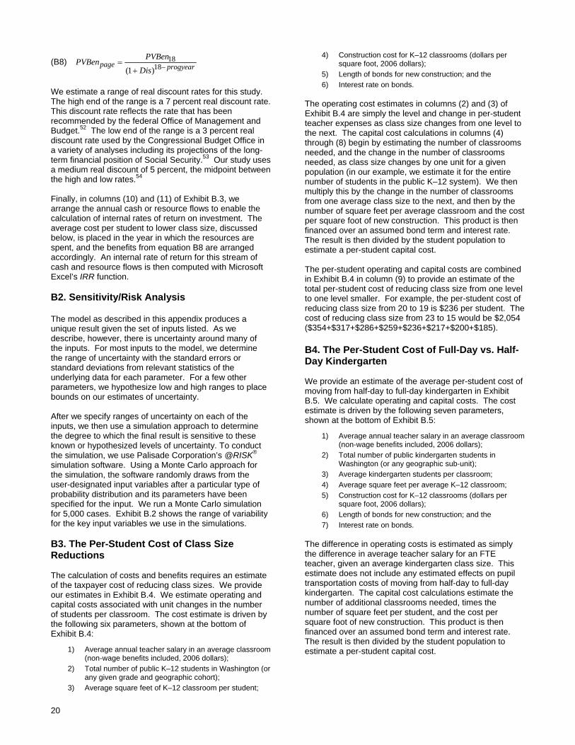
20

(B8) progyearpageDis

PVBenPVBen−+

= 1818

)1(

We estimate a range of real discount rates for this study. The high end of the range is a 7 percent real discount rate. This discount rate reflects the rate that has been recommended by the federal Office of Management and Budget.52 The low end of the range is a 3 percent real discount rate used by the Congressional Budget Office in a variety of analyses including its projections of the long-term financial position of Social Security.53 Our study uses a medium real discount of 5 percent, the midpoint between the high and low rates.54 Finally, in columns (10) and (11) of Exhibit B.3, we arrange the annual cash or resource flows to enable the calculation of internal rates of return on investment. The average cost per student to lower class size, discussed below, is placed in the year in which the resources are spent, and the benefits from equation B8 are arranged accordingly. An internal rate of return for this stream of cash and resource flows is then computed with Microsoft Excel’s IRR function. B2. Sensitivity/Risk Analysis The model as described in this appendix produces a unique result given the set of inputs listed. As we describe, however, there is uncertainty around many of the inputs. For most inputs to the model, we determine the range of uncertainty with the standard errors or standard deviations from relevant statistics of the underlying data for each parameter. For a few other parameters, we hypothesize low and high ranges to place bounds on our estimates of uncertainty. After we specify ranges of uncertainty on each of the inputs, we then use a simulation approach to determine the degree to which the final result is sensitive to these known or hypothesized levels of uncertainty. To conduct the simulation, we use Palisade Corporation’s @RISK® simulation software. Using a Monte Carlo approach for the simulation, the software randomly draws from the user-designated input variables after a particular type of probability distribution and its parameters have been specified for the input. We run a Monte Carlo simulation for 5,000 cases. Exhibit B.2 shows the range of variability for the key input variables we use in the simulations. B3. The Per-Student Cost of Class Size Reductions The calculation of costs and benefits requires an estimate of the taxpayer cost of reducing class sizes. We provide our estimates in Exhibit B.4. We estimate operating and capital costs associated with unit changes in the number of students per classroom. The cost estimate is driven by the following six parameters, shown at the bottom of Exhibit B.4:

1) Average annual teacher salary in an average classroom (non-wage benefits included, 2006 dollars);

2) Total number of public K–12 students in Washington (or any given grade and geographic cohort);

3) Average square feet of K–12 classroom per student;

4) Construction cost for K–12 classrooms (dollars per square foot, 2006 dollars);

5) Length of bonds for new construction; and the 6) Interest rate on bonds.

The operating cost estimates in columns (2) and (3) of Exhibit B.4 are simply the level and change in per-student teacher expenses as class size changes from one level to the next. The capital cost calculations in columns (4) through (8) begin by estimating the number of classrooms needed, and the change in the number of classrooms needed, as class size changes by one unit for a given population (in our example, we estimate it for the entire number of students in the public K–12 system). We then multiply this by the change in the number of classrooms from one average class size to the next, and then by the number of square feet per average classroom and the cost per square foot of new construction. This product is then financed over an assumed bond term and interest rate. The result is then divided by the student population to estimate a per-student capital cost. The per-student operating and capital costs are combined in Exhibit B.4 in column (9) to provide an estimate of the total per-student cost of reducing class size from one level to one level smaller. For example, the per-student cost of reducing class size from 20 to 19 is $236 per student. The cost of reducing class size from 23 to 15 would be $2,054 ($354+$317+$286+$259+$236+$217+$200+$185). B4. The Per-Student Cost of Full-Day vs. Half-Day Kindergarten We provide an estimate of the average per-student cost of moving from half-day to full-day kindergarten in Exhibit B.5. We calculate operating and capital costs. The cost estimate is driven by the following seven parameters, shown at the bottom of Exhibit B.5:

1) Average annual teacher salary in an average classroom (non-wage benefits included, 2006 dollars);

2) Total number of public kindergarten students in Washington (or any geographic sub-unit);

3) Average kindergarten students per classroom; 4) Average square feet per average K–12 classroom; 5) Construction cost for K–12 classrooms (dollars per

square foot, 2006 dollars); 6) Length of bonds for new construction; and the 7) Interest rate on bonds.

The difference in operating costs is estimated as simply the difference in average teacher salary for an FTE teacher, given an average kindergarten class size. This estimate does not include any estimated effects on pupil transportation costs of moving from half-day to full-day kindergarten. The capital cost calculations estimate the number of additional classrooms needed, times the number of square feet per student, and the cost per square foot of new construction. This product is then financed over an assumed bond term and interest rate. The result is then divided by the student population to estimate a per-student capital cost.

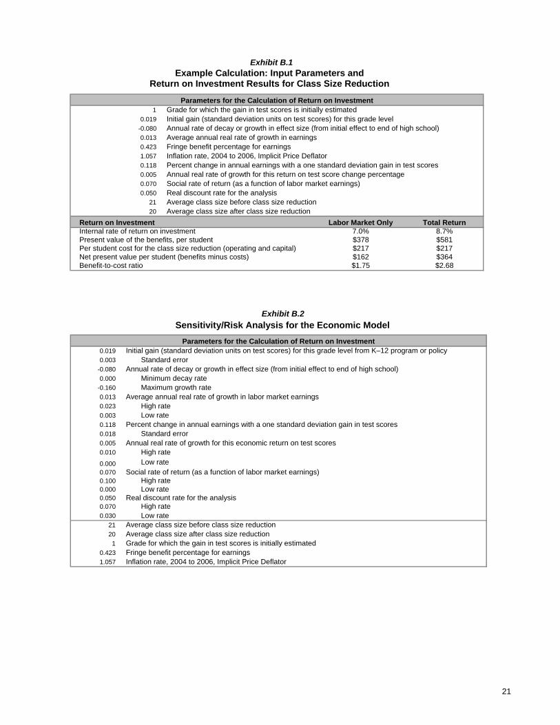
21

1 Grade for which the gain in test scores is initially estimated0.019 Initial gain (standard deviation units on test scores) for this grade level

-0.080 Annual rate of decay or growth in effect size (from initial effect to end of high school) 0.013 Average annual real rate of growth in earnings0.423 Fringe benefit percentage for earnings1.057 Inflation rate, 2004 to 2006, Implicit Price Deflator0.118 Percent change in annual earnings with a one standard deviation gain in test scores 0.005 Annual real rate of growth for this return on test score change percentage 0.070 Social rate of return (as a function of labor market earnings)0.050 Real discount rate for the analysis

21 Average class size before class size reduction20 Average class size after class size reduction

Return on Investment Internal rate of return on investment Present value of the benefits, per student Per student cost for the class size reduction (operating and capital)Net present value per student (benefits minus costs)Benefit-to-cost ratio

Exhibit B.1Example Calculation: Input Parameters and

Return on Investment Results for Class Size Reduction

Labor Market Only Total Return

$162

7.0% 8.7%

Parameters for the Calculation of Return on Investment

$1.75

$581$217$364$2.68

$217$378

0.019 Initial gain (standard deviation units on test scores) for this grade level from K–12 program or policy 0.003 Standard error

-0.080 Annual rate of decay or growth in effect size (from initial effect to end of high school) 0.000 Minimum decay rate

-0.160 Maximum growth rate 0.013 Average annual real rate of growth in labor market earnings0.023 High rate 0.003 Low rate 0.118 Percent change in annual earnings with a one standard deviation gain in test scores 0.018 Standard error 0.005 Annual real rate of growth for this economic return on test scores0.010 High rate 0.000 Low rate 0.070 Social rate of return (as a function of labor market earnings)0.100 High rate 0.000 Low rate 0.050 Real discount rate for the analysis0.070 High rate 0.030 Low rate

21 Average class size before class size reduction20 Average class size after class size reduction1 Grade for which the gain in test scores is initially estimated

0.423 Fringe benefit percentage for earnings1.057 Inflation rate, 2004 to 2006, Implicit Price Deflator

Exhibit B.2Sensitivity/Risk Analysis for the Economic Model

Parameters for the Calculation of Return on Investment

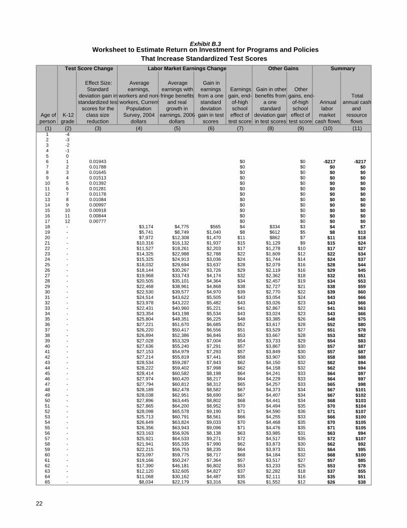
22

(1) (2) (3) (4) (5) (6) (7) (8) (9) (10) (11) 1 -4 2 -3 3 -2 4 -1 5 0 6 1 0.01943 $0 $0 -$217 -$2177 2 0.01788 $0 $0 $0 $08 3 0.01645 $0 $0 $0 $09 4 0.01513 $0 $0 $0 $010 5 0.01392 $0 $0 $0 $011 6 0.01281 $0 $0 $0 $012 7 0.01178 $0 $0 $0 $013 8 0.01084 $0 $0 $0 $014 9 0.00997 $0 $0 $0 $015 10 0.00918 $0 $0 $0 $016 11 0.00844 $0 $0 $0 $017 12 0.00777 $0 $0 $0 $018 - $3,174 $4,775 $565 $4 $334 $3 $4 $719 - $5,741 $8,749 $1,040 $8 $612 $5 $8 $1320 - $7,972 $12,308 $1,470 $11 $862 $7 $11 $1821 - $10,316 $16,132 $1,937 $15 $1,129 $9 $15 $2422 - $11,527 $18,261 $2,203 $17 $1,278 $10 $17 $2723 - $14,325 $22,988 $2,788 $22 $1,609 $12 $22 $3424 - $15,325 $24,913 $3,036 $24 $1,744 $14 $24 $3725 - $18,032 $29,694 $3,637 $28 $2,079 $16 $28 $4426 - $18,144 $30,267 $3,726 $29 $2,119 $16 $29 $4527 - $19,968 $33,743 $4,174 $32 $2,362 $18 $32 $5128 - $20,505 $35,101 $4,364 $34 $2,457 $19 $34 $5329 - $22,468 $38,961 $4,868 $38 $2,727 $21 $38 $5930 - $22,530 $39,577 $4,970 $39 $2,770 $22 $39 $6031 - $24,514 $43,622 $5,505 $43 $3,054 $24 $43 $6632 - $23,978 $43,222 $5,482 $43 $3,026 $23 $43 $6633 - $22,431 $40,960 $5,221 $41 $2,867 $22 $41 $6334 - $23,354 $43,198 $5,534 $43 $3,024 $23 $43 $6635 - $25,804 $48,351 $6,225 $48 $3,385 $26 $48 $7536 - $27,221 $51,670 $6,685 $52 $3,617 $28 $52 $8037 - $26,220 $50,417 $6,556 $51 $3,529 $27 $51 $7838 - $26,894 $52,386 $6,846 $53 $3,667 $28 $53 $8239 - $27,028 $53,329 $7,004 $54 $3,733 $29 $54 $8340 - $27,636 $55,240 $7,291 $57 $3,867 $30 $57 $8741 - $27,153 $54,979 $7,293 $57 $3,849 $30 $57 $8742 - $27,214 $55,819 $7,441 $58 $3,907 $30 $58 $8843 - $28,534 $59,287 $7,943 $62 $4,150 $32 $62 $9444 - $28,222 $59,402 $7,998 $62 $4,158 $32 $62 $9445 - $28,414 $60,582 $8,198 $64 $4,241 $33 $64 $9746 - $27,974 $60,420 $8,217 $64 $4,229 $33 $64 $9747 - $27,794 $60,812 $8,312 $65 $4,257 $33 $65 $9848 - $28,189 $62,478 $8,582 $67 $4,373 $34 $67 $10149 - $28,038 $62,951 $8,690 $67 $4,407 $34 $67 $10250 - $27,896 $63,445 $8,802 $68 $4,441 $34 $68 $10351 - $27,865 $64,200 $8,952 $70 $4,494 $35 $70 $10452 - $28,098 $65,578 $9,190 $71 $4,590 $36 $71 $10753 - $25,713 $60,791 $8,561 $66 $4,255 $33 $66 $10054 - $26,649 $63,824 $9,033 $70 $4,468 $35 $70 $10555 - $26,356 $63,943 $9,096 $71 $4,476 $35 $71 $10556 - $23,163 $56,926 $8,138 $63 $3,985 $31 $63 $9457 - $25,921 $64,533 $9,271 $72 $4,517 $35 $72 $10758 - $21,941 $55,335 $7,990 $62 $3,873 $30 $62 $9259 - $22,215 $56,753 $8,235 $64 $3,973 $31 $64 $9560 - $23,097 $59,775 $8,717 $68 $4,184 $32 $68 $10061 - $19,166 $50,247 $7,364 $57 $3,517 $27 $57 $8562 - $17,390 $46,181 $6,802 $53 $3,233 $25 $53 $7863 - $12,120 $32,605 $4,827 $37 $2,282 $18 $37 $5564 - $11,068 $30,162 $4,487 $35 $2,111 $16 $35 $5165 - $8,034 $22,179 $3,316 $26 $1,552 $12 $26 $38

Gain in earnings

from a one standard deviation

gain in test scores

Exhibit B.3Worksheet to Estimate Return on Investment for Programs and Policies

That Increase Standardized Test Scores

Age of person

K-12 grade

Average earnings,

workers and non- workers, Current

Population Survey, 2004

dollars

Average earnings with fringe benefits

and real growth in

earnings, 2006 dollars

Effect Size: Standard

deviation gain in standardized test

scores for the class size reduction

Test Score Change Labor Market Earnings Change

Total annual cash

and resource

flows

Earnings gain, end-

of-high school

effect of test score

Gain in other benefits from

a one standard

deviation gain in test scores

Other gains, end-

of-high school

effect of test score

Other Gains Summary

Annual labor

market cash flows

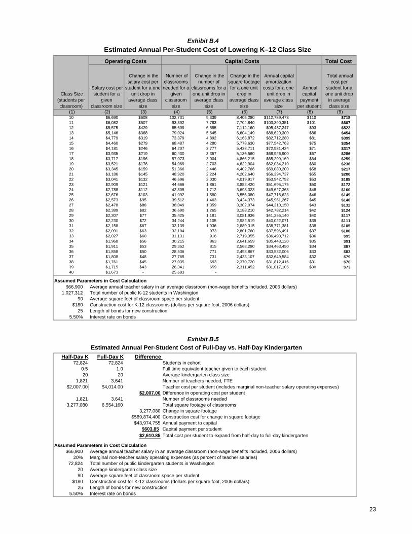
23

Total Cost

(1) (2) (3) (4) (5) (6) (7) (8) (9) 10 $6,690 $608 102,731 9,339 8,405,280 $112,789,473 $110 $71811 $6,082 $507 93,392 7,783 7,704,840 $103,390,351 $101 $60712 $5,575 $429 85,609 6,585 7,112,160 $95,437,247 $93 $52213 $5,146 $368 79,024 5,645 6,604,149 $88,620,300 $86 $45414 $4,779 $319 73,379 4,892 6,163,872 $82,712,280 $81 $39915 $4,460 $279 68,487 4,280 5,778,630 $77,542,763 $75 $35416 $4,181 $246 64,207 3,777 5,438,711 $72,981,424 $71 $31717 $3,935 $219 60,430 3,357 5,136,560 $68,926,900 $67 $28618 $3,717 $196 57,073 3,004 4,866,215 $65,299,169 $64 $25919 $3,521 $176 54,069 2,703 4,622,904 $62,034,210 $60 $23620 $3,345 $159 51,366 2,446 4,402,766 $59,080,200 $58 $21721 $3,186 $145 48,920 2,224 4,202,640 $56,394,737 $55 $20022 $3,041 $132 46,696 2,030 4,019,917 $53,942,792 $53 $18523 $2,909 $121 44,666 1,861 3,852,420 $51,695,175 $50 $17224 $2,788 $112 42,805 1,712 3,698,323 $49,627,368 $48 $16025 $2,676 $103 41,092 1,580 3,556,080 $47,718,623 $46 $14926 $2,573 $95 39,512 1,463 3,424,373 $45,951,267 $45 $14027 $2,478 $88 38,049 1,359 3,302,074 $44,310,150 $43 $13228 $2,389 $82 36,690 1,265 3,188,210 $42,782,214 $42 $12429 $2,307 $77 35,425 1,181 3,081,936 $41,356,140 $40 $11730 $2,230 $72 34,244 1,105 2,982,519 $40,022,071 $39 $11131 $2,158 $67 33,139 1,036 2,889,315 $38,771,381 $38 $10532 $2,091 $63 32,104 973 2,801,760 $37,596,491 $37 $10033 $2,027 $60 31,131 916 2,719,355 $36,490,712 $36 $9534 $1,968 $56 30,215 863 2,641,659 $35,448,120 $35 $9135 $1,911 $53 29,352 815 2,568,280 $34,463,450 $34 $8736 $1,858 $50 28,536 771 2,498,867 $33,532,006 $33 $8337 $1,808 $48 27,765 731 2,433,107 $32,649,584 $32 $7938 $1,761 $45 27,035 693 2,370,720 $31,812,416 $31 $7639 $1,715 $43 26,341 659 2,311,452 $31,017,105 $30 $7340 $1,673 - 25,683 -

Assumed Parameters in Cost Calculation $66,900 Average annual teacher salary in an average classroom (non-wage benefits included, 2006 dollars)

1,027,312 Total number of public K-12 students in Washington 90 Average square feet of classroom space per student

$180 Construction cost for K-12 classrooms (dollars per square foot, 2006 dollars)25 Length of bonds for new construction

5.50% Interest rate on bonds

Half-Day K Full-Day K Difference 72,824 72,824 Students in cohort

0.5 1.0 Full time equivalent teacher given to each student20 20 Average kindergarten class size

1,821 3,641 Number of teachers needed, FTE$2,007.00 $4,014.00 Teacher cost per student (includes marginal non-teacher salary operating expenses)

$2,007.00 Difference in operating cost per student1,821 3,641 Number of classrooms needed

3,277,080 6,554,160 Total square footage of classrooms3,277,080 Change in square footage

$589,874,400 Construction cost for change in square footage$43,974,755 Annual payment to capital

$603.85 Capital payment per student$2,610.85 Total cost per student to expand from half-day to full-day kindergarten

Assumed Parameters in Cost Calculation $66,900 Average annual teacher salary in an average classroom (non-wage benefits included, 2006 dollars)

20% Marginal non-teacher salary operating expenses (as percent of teacher salaries) 72,824 Total number of public kindergarten students in Washington

20 Average kindergarten class size 90 Average square feet of classroom space per student

$180 Construction cost for K-12 classrooms (dollars per square foot, 2006 dollars)25 Length of bonds for new construction

5.50% Interest rate on bonds

Exhibit B.5Estimated Annual Per-Student Cost of Full-Day vs. Half-Day Kindergarten

Exhibit B.4Estimated Annual Per-Student Cost of Lowering K–12 Class Size

Class Size (students per classroom)

Capital CostsOperating Costs

Salary cost per student for a

given classroom size

Number of classrooms needed for a

given classroom

size

Change in the number of

classrooms for a one unit drop in average class

size

Change in the salary cost per

student for a one unit drop in

average class size

Change in the square footage for a one unit

drop in average class

size

Annual capital amortization

costs for a one unit drop in

average class size

Annual capital

payment per student

Total annual cost per

student for a one unit drop

in average class size

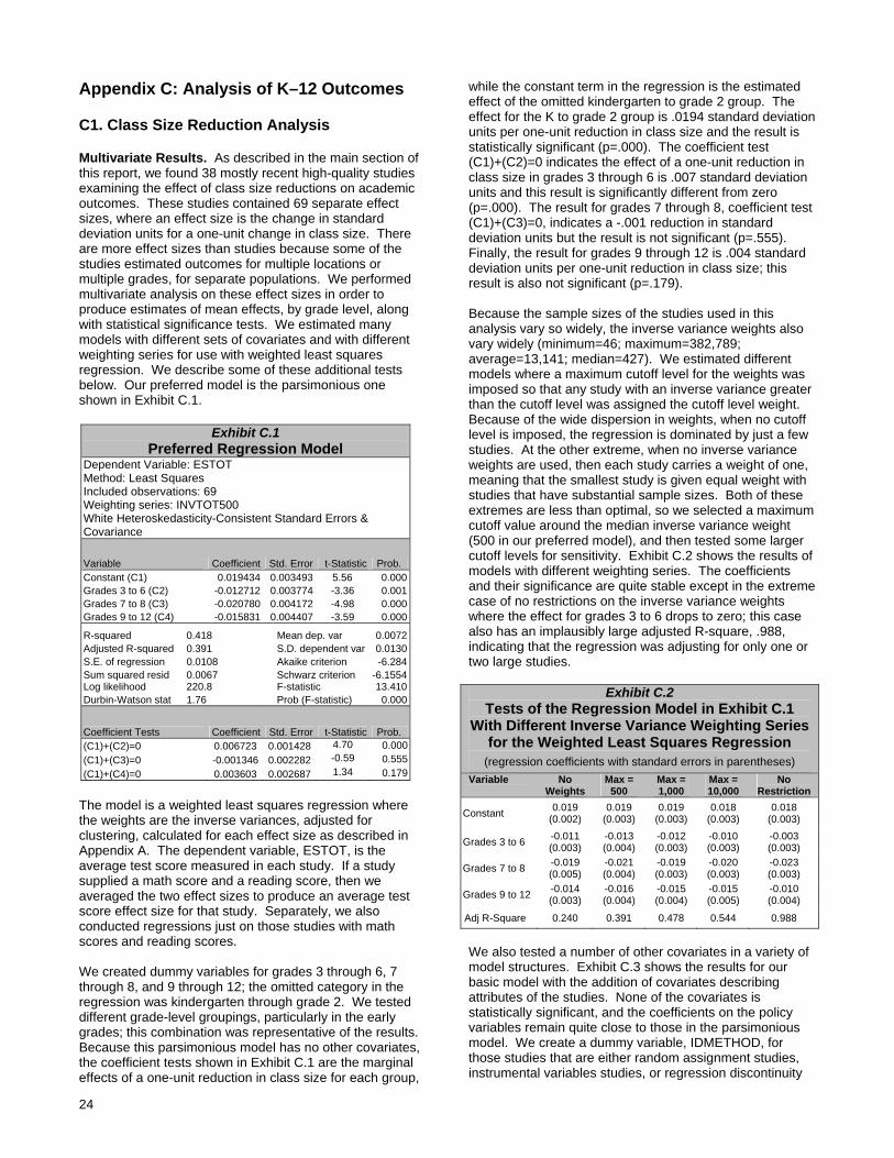
24

Appendix C: Analysis of K–12 Outcomes C1. Class Size Reduction Analysis Multivariate Results. As described in the main section of this report, we found 38 mostly recent high-quality studies examining the effect of class size reductions on academic outcomes. These studies contained 69 separate effect sizes, where an effect size is the change in standard deviation units for a one-unit change in class size. There are more effect sizes than studies because some of the studies estimated outcomes for multiple locations or multiple grades, for separate populations. We performed multivariate analysis on these effect sizes in order to produce estimates of mean effects, by grade level, along with statistical significance tests. We estimated many models with different sets of covariates and with different weighting series for use with weighted least squares regression. We describe some of these additional tests below. Our preferred model is the parsimonious one shown in Exhibit C.1.

Exhibit C.1 Preferred Regression Model

Dependent Variable: ESTOT Method: Least Squares Included observations: 69 Weighting series: INVTOT500 White Heteroskedasticity-Consistent Standard Errors & Covariance

Variable Coefficient Std. Error t-Statistic Prob. Constant (C1) 0.019434 0.003493 5.56 0.000Grades 3 to 6 (C2) -0.012712 0.003774 -3.36 0.001Grades 7 to 8 (C3) -0.020780 0.004172 -4.98 0.000Grades 9 to 12 (C4) -0.015831 0.004407 -3.59 0.000

R-squared 0.418 Mean dep. var 0.0072Adjusted R-squared 0.391 S.D. dependent var 0.0130S.E. of regression 0.0108 Akaike criterion -6.284Sum squared resid 0.0067 Schwarz criterion -6.1554Log likelihood 220.8 F-statistic 13.410Durbin-Watson stat 1.76 Prob (F-statistic) 0.000

Coefficient Tests Coefficient Std. Error t-Statistic Prob. (C1)+(C2)=0 0.006723 0.001428 4.70 0.000(C1)+(C3)=0 -0.001346 0.002282 -0.59 0.555(C1)+(C4)=0 0.003603 0.002687 1.34 0.179

The model is a weighted least squares regression where the weights are the inverse variances, adjusted for clustering, calculated for each effect size as described in Appendix A. The dependent variable, ESTOT, is the average test score measured in each study. If a study supplied a math score and a reading score, then we averaged the two effect sizes to produce an average test score effect size for that study. Separately, we also conducted regressions just on those studies with math scores and reading scores. We created dummy variables for grades 3 through 6, 7 through 8, and 9 through 12; the omitted category in the regression was kindergarten through grade 2. We tested different grade-level groupings, particularly in the early grades; this combination was representative of the results. Because this parsimonious model has no other covariates, the coefficient tests shown in Exhibit C.1 are the marginal effects of a one-unit reduction in class size for each group,

while the constant term in the regression is the estimated effect of the omitted kindergarten to grade 2 group. The effect for the K to grade 2 group is .0194 standard deviation units per one-unit reduction in class size and the result is statistically significant (p=.000). The coefficient test (C1)+(C2)=0 indicates the effect of a one-unit reduction in class size in grades 3 through 6 is .007 standard deviation units and this result is significantly different from zero (p=.000). The result for grades 7 through 8, coefficient test (C1)+(C3)=0, indicates a -.001 reduction in standard deviation units but the result is not significant (p=.555). Finally, the result for grades 9 through 12 is .004 standard deviation units per one-unit reduction in class size; this result is also not significant (p=.179). Because the sample sizes of the studies used in this analysis vary so widely, the inverse variance weights also vary widely (minimum=46; maximum=382,789; average=13,141; median=427). We estimated different models where a maximum cutoff level for the weights was imposed so that any study with an inverse variance greater than the cutoff level was assigned the cutoff level weight. Because of the wide dispersion in weights, when no cutoff level is imposed, the regression is dominated by just a few studies. At the other extreme, when no inverse variance weights are used, then each study carries a weight of one, meaning that the smallest study is given equal weight with studies that have substantial sample sizes. Both of these extremes are less than optimal, so we selected a maximum cutoff value around the median inverse variance weight (500 in our preferred model), and then tested some larger cutoff levels for sensitivity. Exhibit C.2 shows the results of models with different weighting series. The coefficients and their significance are quite stable except in the extreme case of no restrictions on the inverse variance weights where the effect for grades 3 to 6 drops to zero; this case also has an implausibly large adjusted R-square, .988, indicating that the regression was adjusting for only one or two large studies.

Exhibit C.2 Tests of the Regression Model in Exhibit C.1

With Different Inverse Variance Weighting Series for the Weighted Least Squares Regression

(regression coefficients with standard errors in parentheses) Variable No

Weights Max =

500 Max = 1,000

Max = 10,000

No Restriction

Constant 0.019 (0.002)

0.019 (0.003)

0.019 (0.003)

0.018 (0.003)

0.018 (0.003)

Grades 3 to 6 -0.011 (0.003)

-0.013 (0.004)

-0.012 (0.003)

-0.010 (0.003)

-0.003 (0.003)

Grades 7 to 8 -0.019 (0.005)

-0.021 (0.004)

-0.019 (0.003)

-0.020 (0.003)

-0.023 (0.003)

Grades 9 to 12 -0.014 (0.003)

-0.016 (0.004)

-0.015 (0.004)

-0.015 (0.005)

-0.010 (0.004)

Adj R-Square 0.240 0.391 0.478 0.544 0.988

We also tested a number of other covariates in a variety of model structures. Exhibit C.3 shows the results for our basic model with the addition of covariates describing attributes of the studies. None of the covariates is statistically significant, and the coefficients on the policy variables remain quite close to those in the parsimonious model. We create a dummy variable, IDMETHOD, for those studies that are either random assignment studies, instrumental variables studies, or regression discontinuity

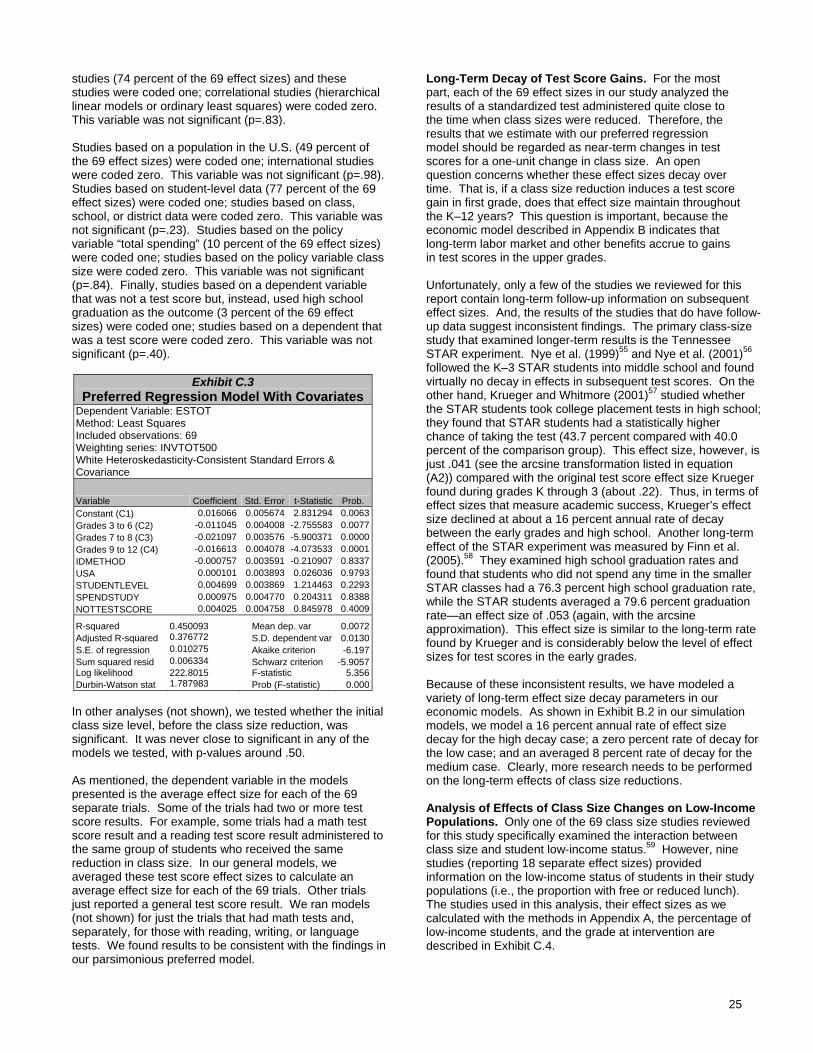
25

studies (74 percent of the 69 effect sizes) and these studies were coded one; correlational studies (hierarchical linear models or ordinary least squares) were coded zero. This variable was not significant (p=.83). Studies based on a population in the U.S. (49 percent of the 69 effect sizes) were coded one; international studies were coded zero. This variable was not significant (p=.98). Studies based on student-level data (77 percent of the 69 effect sizes) were coded one; studies based on class, school, or district data were coded zero. This variable was not significant (p=.23). Studies based on the policy variable “total spending” (10 percent of the 69 effect sizes) were coded one; studies based on the policy variable class size were coded zero. This variable was not significant (p=.84). Finally, studies based on a dependent variable that was not a test score but, instead, used high school graduation as the outcome (3 percent of the 69 effect sizes) were coded one; studies based on a dependent that was a test score were coded zero. This variable was not significant (p=.40).

Exhibit C.3 Preferred Regression Model With Covariates

Dependent Variable: ESTOT Method: Least Squares Included observations: 69 Weighting series: INVTOT500 White Heteroskedasticity-Consistent Standard Errors & Covariance

Variable Coefficient Std. Error t-Statistic Prob. Constant (C1) 0.016066 0.005674 2.831294 0.0063Grades 3 to 6 (C2) -0.011045 0.004008 -2.755583 0.0077Grades 7 to 8 (C3) -0.021097 0.003576 -5.900371 0.0000Grades 9 to 12 (C4) -0.016613 0.004078 -4.073533 0.0001IDMETHOD -0.000757 0.003591 -0.210907 0.8337USA 0.000101 0.003893 0.026036 0.9793STUDENTLEVEL 0.004699 0.003869 1.214463 0.2293SPENDSTUDY 0.000975 0.004770 0.204311 0.8388NOTTESTSCORE 0.004025 0.004758 0.845978 0.4009

R-squared 0.450093 Mean dep. var 0.0072Adjusted R-squared 0.376772 S.D. dependent var 0.0130S.E. of regression 0.010275 Akaike criterion -6.197Sum squared resid 0.006334 Schwarz criterion -5.9057Log likelihood 222.8015 F-statistic 5.356Durbin-Watson stat 1.787983 Prob (F-statistic) 0.000

In other analyses (not shown), we tested whether the initial class size level, before the class size reduction, was significant. It was never close to significant in any of the models we tested, with p-values around .50. As mentioned, the dependent variable in the models presented is the average effect size for each of the 69 separate trials. Some of the trials had two or more test score results. For example, some trials had a math test score result and a reading test score result administered to the same group of students who received the same reduction in class size. In our general models, we averaged these test score effect sizes to calculate an average effect size for each of the 69 trials. Other trials just reported a general test score result. We ran models (not shown) for just the trials that had math tests and, separately, for those with reading, writing, or language tests. We found results to be consistent with the findings in our parsimonious preferred model.

Long-Term Decay of Test Score Gains. For the most part, each of the 69 effect sizes in our study analyzed the results of a standardized test administered quite close to the time when class sizes were reduced. Therefore, the results that we estimate with our preferred regression model should be regarded as near-term changes in test scores for a one-unit change in class size. An open question concerns whether these effect sizes decay over time. That is, if a class size reduction induces a test score gain in first grade, does that effect size maintain throughout the K–12 years? This question is important, because the economic model described in Appendix B indicates that long-term labor market and other benefits accrue to gains in test scores in the upper grades. Unfortunately, only a few of the studies we reviewed for this report contain long-term follow-up information on subsequent effect sizes. And, the results of the studies that do have follow-up data suggest inconsistent findings. The primary class-size study that examined longer-term results is the Tennessee STAR experiment. Nye et al. (1999)55 and Nye et al. (2001)56 followed the K–3 STAR students into middle school and found virtually no decay in effects in subsequent test scores. On the other hand, Krueger and Whitmore (2001)57 studied whether the STAR students took college placement tests in high school; they found that STAR students had a statistically higher chance of taking the test (43.7 percent compared with 40.0 percent of the comparison group). This effect size, however, is just .041 (see the arcsine transformation listed in equation (A2)) compared with the original test score effect size Krueger found during grades K through 3 (about .22). Thus, in terms of effect sizes that measure academic success, Krueger’s effect size declined at about a 16 percent annual rate of decay between the early grades and high school. Another long-term effect of the STAR experiment was measured by Finn et al. (2005).58 They examined high school graduation rates and found that students who did not spend any time in the smaller STAR classes had a 76.3 percent high school graduation rate, while the STAR students averaged a 79.6 percent graduation rate—an effect size of .053 (again, with the arcsine approximation). This effect size is similar to the long-term rate found by Krueger and is considerably below the level of effect sizes for test scores in the early grades. Because of these inconsistent results, we have modeled a variety of long-term effect size decay parameters in our economic models. As shown in Exhibit B.2 in our simulation models, we model a 16 percent annual rate of effect size decay for the high decay case; a zero percent rate of decay for the low case; and an averaged 8 percent rate of decay for the medium case. Clearly, more research needs to be performed on the long-term effects of class size reductions. Analysis of Effects of Class Size Changes on Low-Income Populations. Only one of the 69 class size studies reviewed for this study specifically examined the interaction between class size and student low-income status.59 However, nine studies (reporting 18 separate effect sizes) provided information on the low-income status of students in their study populations (i.e., the proportion with free or reduced lunch). The studies used in this analysis, their effect sizes as we calculated with the methods in Appendix A, the percentage of low-income students, and the grade at intervention are described in Exhibit C.4.

26

Exhibit C.4

Data From Studies Describing the Proportion of Students in Low-Income Families

Study Average Effect Size

Percent Low-income Grade

Akerhielm (1995) 0.0034 39.3 8 Ecalle et al (2006) 0.0137 24.0 1 Feinstein & Symons (1999) 0.0038 25.0 10 Hoxby (2000) 0.0014 24.9 2 Hoxby (2000) -0.0007 24.9 3 Hoxby (2000) 0.0001 24.9 2 Hoxby (2000) 0.0000 24.9 4 Krueger (1999) 0.0275 47.0 0 Krueger (1999) 0.0404 59.0 1 Krueger (1999) 0.0266 66.0 2 Krueger (1999) 0.0229 60.0 3 Levacic et al (2005) -0.0019 13.0 8 Levacic et al (2005) 0.0055 11.8 9.5 Molnar et al (1999) 0.0196 57.7 1 Molnar et al (1999) 0.0173 54.0 1 NICHD (2004) 0.0174 32.2 1 Sander (1999) 0.0014 20.9 8 Sander (1999) 0.0022 23.0 3

We performed multivariate analyses on these effect sizes in order to produce estimates of effects by low-income status and perform tests of significance. The model is a weighted least squares regression where the weights are the inverse variances (see the discussion in C1, Multivariate Results), adjusted for clustering, calculated for each effect size as described in Appendix A. The dependent variable, ESTOT, is the average effect size, also described earlier. There were too few observations to model math and reading scores separately. The independent variables are percentages of students receiving free or reduced lunch (LowSES) and the grade at which class size was reduced (Grade). The results of a linear model using LowSES and Grade to predict ESTOT, summarized in Exhibit C.5, show that LowSES has a significant positive effect on ESTOT (p=.0015) even after controlling for grade level. A scatter plot of ESTOT and LowSES (Exhibit 4) indicates a curvilinear relationship, so a squared LowSES term was added to the model. The results of this model are summarized in Exhibit C.6. Individually, the LowSES and LowSES2 covariates are not statistically significant. Tested jointly, however, they are significant at p=0.0042. Exhibit C.7 illustrates the effect sizes predicted by the curvilinear model (in black) and the linear model (in blue), while holding grade level constant at 3.79 (the mean value for grade level in the model). Actual values are represented in red. While there is no compelling reason to pick one model over the other, they point towards the same general conclusion, that, all things equal, class size reductions are more effective for classes comprising low-income students than for other students. Using the curvilinear results, the effect on achievement of a one-student reduction in class size for a class with 40 percent low-income students is more than double that of a class with 20 percent low-income students (.011 and .005 respectively)

Exhibit C.5

Linear Model Dependent Variable: ESTOT Method: Least Squares Included observations: 18 Weighting series: INVTOT500

Variable Coefficient Std. Error t-Statistic Prob. Constant -0.00224 0.00702 -.32 0.7538LowSES 0.004821 0.000125 3.87 0.0015Grade -0.000726 0.000653 -1.11 0.2834

R-squared 0.7151 Mean dep. var 0.0137Adjusted R-squared 0.6771 S.D. dependent var 0.0124S.E. of regression 0.14131 F-statistic 18.82Sum squared resid 0.75166 Prob (F-statistic) 0.0001

Exhibit C.6 Curvilinear Model

Dependent Variable: ESTOT Method: Least Squares Included observations: 18 Weighting series: INVTOT500

Variable Coefficient Std. Error t-Statistic Prob. Constant 0.00967 0.01250 .77 0.4519LowSES2 0.0000087 0.000076 1.15 0.2706LowSES -0.0002180 0.000632 -0.35 0.7315Grade -0.0009336 0.000670 -1.39 0.1857

R-squared 0.7395 Mean dep. var 0.0137Adjusted R-squared 0.6837 S.D. dependent var 0.0124S.E. of regression 0.13985 F-statistic 13.25Sum squared resid 0.2738 Prob (F-statistic) 0.0002

Joint Significance Tests F-statistic Prob. LowSES and LowSES2 8.31 0.0042LowSES and LowSES2 and Grade 13.25 0.0002

Exhibit C.7Change in Acheivement From Reducing Class Size: Predicted by Student Low-Income Status

-.005.000.005.010.015.020.025.030.035.040.045

5 25 45 65Percent of Low-Income Students

Effe

ct S

ize

27

C2. Full-Day vs. Half-Day Kindergarten This exhibit provides more information on the effect sizes for full-day kindergarten at various follow-up periods.

Exhibit C.8 Effect Sizes At the End of Kindergarten and

In The Early Years of Education (Maximum inverse variance weight set at 500)

Follow-up

K Grade 1 Grade 2

or 3 Grade 4

or 5 Effect size 0.1805 0.0108 0.0477 0.0004 Standard Error on Effect Size 0.02874 0.0375 0.0300 0.0310 Upper limit with 95% confidence 0.2370 0.0840 0.1060 0.0600 Lower limit with 95% confidence 0.1242 -0.0628 -0.0111 -0.0612

Number of Effect Sizes 17 6 5 4 Endnotes 1 ESSB 6386 §607(15), Chapter 372, Laws of 2006. 2 Washington Learns Steering Committee. (2006). Washington Learns: World class, learner-focused, seamless education. Olympia: Washington Learns, pp. 7-8. 3 See: (a) S. Aos, M. Miller, & E. Drake. (2006). Evidence-Based Public Policy Options to Reduce Future Prison Construction, Criminal Justice Costs, and Crime Rates. Olympia: Washington State Institute for Public Policy; (b) S. Aos, M. Miller, & E. Drake. (2006). Evidence-based adult corrections programs. Olympia: Washington State Institute for Public Policy; (c) S. Aos, J. Mayfield, M. Miller, & W. Yen. (2006). Evidence-based treatment of alcohol, drug, and mental health disorders: Potential benefits, costs, and fiscal impacts for Washington State. Olympia: Washington State Institute for Public Policy; (d) S. Aos, R. Lieb, J. Mayfield, M. Miller, & A. Pennucci. (2004). Benefits and costs of prevention and early intervention programs for youth. Olympia: Washington State Institute for Public Policy; and (e) S. Aos, P. Phipps, R. Barnoski, & R. Lieb. (2001). The comparative costs and benefits of programs to reduce crime. Olympia: Washington State Institute for Public Policy. 4 See: F. Cunha, J. Heckman, L. Lochner, & D. Masterov. (2005). Interpreting the evidence on life cycle skill formation. In Handbook of the Economics of Education, E. Hanushek & F. Welch (Eds.), North-Holland. See also: W. Riddell. (2006). The impact of education on economic and social outcomes: An overview of recent advances in economics. University of British Columbia: Department of Economics. 5 As described in the appendix, we calculate mean-difference effect sizes for each study and then meta-analyze these individual effect sizes to produce an average effect size for a group of studies on a particular topic. In general, we follow the procedures in M.W. Lipsey & D. Wilson. (2001). Practical meta-analysis. Thousand Oaks: Sage Publications. Many studies of education topics, however, are based on data that are organized hierarchically: students are nested in classes, classes are nested in schools, and schools are nested in districts. To account for this, we adjust effect sizes and inverse variance weights using methods suggested in L.V. Hedges. (2006). Effect sizes in cluster-randomized designs. Institute for Policy Research, Northwestern University, Working Paper Series manuscript.

6 The disagreements between Hanushek and Krueger over the effectiveness of policies can be seen in: L. Mishel & R. Rothstein (Eds.). (2002). The class size debate. Washington DC: Economic Policy Institute. On the other hand, the agreements between these two economists on how to calculate benefits of any statistically significant effect can be seen in: A. Krueger. (2003). Economic considerations and class size. The Economic Journal, 113: F34-F64; and E.A. Hanushek. (2004). The economic value of improving local schools, downloaded from: <http://edpro.stanford.edu/Hanushek/admin/pages/files/uploads/Economic%20Value.cleveland%20fed.pdf>. 7 See: Hanushek (2004), citing the work of R.J. Murnane, J.B. Willett, Y. Duhaldeborde, & J.H. Tyler. (2000). How important are the cognitive skills of teenagers in predicting subsequent earnings? Journal of Policy Analysis and Management, 19(4): 547-568. See also: J. Currie & D. Thomas. (2001). Early test scores, school quality and SES: Longrun effects on wage and employment outcomes. Research in Labor Economics, 20: 103-132. 8 For a review of this literature see: W.C. Riddell. (2006). The impact of education on economic and social outcomes: An overview of recent advances in economics. University of British Columbia: Department of Economics. 9 For a review of the issues in the debate, see: L. Mishel & R. Rothstein (Eds.). (2002). The class size debate. Washington DC: Economic Policy Institute. See also the opposing arguments in: R. Greenwald, L.V. Hedges, & R.D. Laine. (1996). The effect of school resources on student achievement. Review of Educational Research, 66(3): 361-396. E.A. Hanushek. (1996). A more complete picture of school resource policies. Review of Educational Research, 66(3): 361-396. 10 For example, in 2000 Washington voters passed Initiative 728 (72 percent yes vote) authorizing additional funding for reduced class size, extended learning programs, educator professional development, and facility improvements. 11 For a summary, see: R. Ehrenberg, D.J. Brewer, A. Gamoran, & J.D. Willms. (2001). Class size and student achievement. Psychological Science, 2(1): 1-30. 12 A.B. Krueger. (1999). Experimental estimates of education production functions. Quarterly Journal of Economics, 114(2): 497-532. A.B. Krueger & D.M. Whitmore. (2001). The effect of attending a small class in the early grades on college-test taking and middle school test results: Evidence from Project STAR. Economic Journal, 111(468): 1-28. 13 For a study questioning some of the STAR findings, see: E.A. Hanushek. (1999). Some findings from an independent investigation of the Tennessee STAR experiment and from other investigations of class size effects. Educational Evaluation and Policy Analysis, 21(2): 143-168. 14 The two studies that analyzed the same dataset for STAR are: A. Krueger. (1999). Experimental estimates of education production functions. Quarterly Journal of Economics, 114(2: 497-532; and C. Kang. (2005). Effects of small classes on academic achievement: Evidence from new entrants to Project STAR. Singapore: National University of Singapore, Department of Economics. 15 For small changes greater than a one-unit drop in class size, our effect sizes can be multiplied by the class size change to approximate the total effect. To date, only a few analysts have tried to estimate non-linear relationships between class size and test scores; see Borland et al. (2005). 16 The average return and the range were computed from the simulation model. The range was set to include 1.5 standard deviations above and below the mean level of returns in the 5,000 case simulation. 17 The long-term nominal rate of return on the S&P 500 is about 7.4 percent per year. After adjusting for inflation, the real rate is about 4.4 percent. 18 M. Oelerich. (1984). Should kindergarten children attend school all day every day? The Journal of the College of Education, Fall: 13-16 (ERIC No. ED254318). 19 Ibid.

28

20 K. Kauerz. (2005). Full day kindergarten: A study of state policies in the United States. Denver, CO: Education Commission of the States. 21 Ibid. 22 Preliminary findings from the 2007 Washington State full-day kindergarten survey. Personal communication with Debra Williams-Appleton, Office of Superintendent of Public Instruction, March 2, 2007. 23 Complete information on the ECLS-K is available on the website of National Center for Education Statistics: <http://nces.ed.gov/ecls/kindergarten.asp>. 24 V.E. Lee, & D.T. Burkam. (2002). Inequality at the starting gate: Social background differences in achievement as children begin school. Washington, DC: Economic Policy Institute. 25 Because not all studies provided information on demographics, we are unable to split the studies into advantaged vs. disadvantaged children. 26 More detailed information about these effect sizes is provided in Appendix C2. 27 These groups are derived from several papers. Head Start: Nielsen & Cooper-Martin (2002) analyzed results separately for children who attended the local Head Start program the year before kindergarten. In the Head Start group, 92 percent belonged to racial or ethnic minorities and 83 percent qualified for free or reduced lunch. Minority status: DeCicca (2006) analyzed results through the end of first grade for Black and Hispanic children separately. Poverty: Cannon, et al. (2006) analyzed results through third grade for children with family income below the federal poverty level. Saam & Nowak (2005) analyzed results at third grade for children eligible for free lunch. DeCicca and Cannon, et al. used data from the Early Childhood Longitudinal Study-Kindergarten (ECLS-K). 28 We follow the meta-analytic methods described in M.W. Lipsey, & D. Wilson. (2001). Practical meta-analysis. Thousand Oaks: Sage Publications. 29 D. Webbink (2005). Causal effects in education. Journal of Economic Surveys, 19(4): 535-560. 30 See: Identifying and implementing education practices supported by rigorous evidence: A user friendly guide (2003, December) Coalition for Evidence-Based Policy, U.S. Department of Education, Institute of Education Sciences, National Center for Education Evaluation and Regional Assistance. Available at: <http://www.evidencebasedpolicy.org/docs/Identifying_and_Implementing_Educational_Practices.pdf>. 31 Lipsey & Wilson (2001), Table B10, equation 22, p. 200. 32 Ibid., Table B10, equation 1, p. 198>. 33 L.V. Hedges. (1981). Distribution theory for Glass’s estimator of effect size and related estimators. Journal of Educational Statistics, 6: 107-128. 34 Lipsey & Wilson (2001), equation 3.22, p. 49. 35 These formulas are taken from: L.V. Hedges. (2007). Effect sizes in cluster-randomized designs. Manuscript downloaded from the author’s website, cited with permission of the author. 36 Lipsey & Wilson (2001), equation 3.23, p. 49. 37 Ibid., equation 3.24, p. 49. 38 Ibid., p. 114. 39 Ibid. 40 Ibid. 41 Ibid., p. 116. 42 Ibid., p. 134. 43 See, for example: A. Krueger. (2003). Economic considerations and class size. The Economic Journal, 113: F34-F64; and E.A. Hanushek. (2004). The economic value of improving local schools, downloaded from <http://edpro.stanford.edu/Hanushek/admin/pages/files/ uploads/Economic%20Value.cleveland%20fed.pdf>. 44 W.C. Riddell. (2006). The impact of education on economic and social outcomes: An overview of recent advances in economics. University of British Columbia: Department of Economics.

45 Current Population Survey data downloaded from the U.S. Census Bureau site with the DataFerrett extraction utility: <http://www.bls.census.gov/cps/cpsmain.htm>. 46 Washington State Economic and Revenue Forecast Council: <http://www.erfc.wa.gov/pubs/nov06pub.pdf>. 47 United State Bureau of Labor Statistics, Employment Cost Index, March 14, 2006 release, data for December 2005: <http://www.bls.gov/news.release/ecec.toc.htm>. 48 See Congressional Budget Office data for the June 2006 report, Table W-5, at: <http://www.cbo.gov/ftpdocs/72xx/doc7289/06-14-SupplementalData.xls>. 49 Our estimated return and standard error of the return are calculated from the findings in: R.J. Murnane, J.B. Willett, Y. Duhaldeborde, & J.H. Tyler. (2000). How important are the cognitive skills of teenagers in predicting subsequent earnings? Journal of Policy Analysis and Management, 19(4): 547-568. This study and others are also reviewed in: E.A. Hanushek. (2004). The economic value of improving local schools, pg 6. downloaded from: <http://edpro.stanford.edu/Hanushek/admin/pages/files/uploads/Economic%20Value.cleveland%20fed.pdf>. 50 Hanushek (2004), p. 7. 51 B. Wolfe & R. Haveman. (2002). Social and nonmarket benefits from education in an advanced economy. “Proceedings from the Federal Reserve Bank of Boston's 47th economic conference,” Education in the 21st Century: Meeting the Challenges of a Changing World, accessed from: <http://www.bos.frb.org/ economic/conf/conf47/index.htm>. See also a collection of articles on the topic published in J. Behrman & N. Stacey (Eds.). (1997). The social benefits of education. Ann Arbor: The University of Michigan Press. See also: W.C. Riddell. (2006). The impact of education on economic and social outcomes: An overview of recent advances in economics. University of British Columbia: Department of Economics. 52 Office of Management and Budget, Circular A-94 (revised 1992). 53 See Congressional Budget Office report: <http://www.cbo.gov/ ftpdocs/72xx/doc7289/06-14-LongTermProjections.pdf>. 54 For a general discussion of discount rates for applied public benefit-cost analyses, see: C. Bazelon & K. Smetters. (1999). Discounting inside the Washington D.C. Beltway. Journal of Economic Perspectives, 13(4): 213-28. See also: H. Kohyama. (2006). Selecting discount rates for budgetary purposes, Briefing Paper No. 29. <http://www.law.harvard.edu/faculty/hjackson/ DiscountRates_29.pdf>. 55 B. Nye, L. Hedges, & S. Konstantopoulos. (1999). The long-term effects of small classes: A five-year follow-up of the Tennessee class size experiment. Educational Evaluation and Policy Analysis, 21(2): 127-142. 56 B. Nye, L. Hedges, & S. Konstantopoulos. (2001). The long-term effects of small classes in early grades: Lasting benefits in mathematics achievement at grade 9. The Journal of Experimental Education, 69(3): 245-257. 57 A. Krueger, & D. Whitmore. (2001). The effect of attending a small class in the early grades on college-test taking and middle school test results: Evidence from project star. The Economic Journal, 111(January): 1-28. 58 J. Finn, S. Gerber, & J. Boyd-Zaharias. (2005). Small classes in the early grades, academic achievement, and graduating from high school. Journal of Educational Psychology, 97(2): 214-223. 59 Krueger (1999).

Document No. 07-03-2201