was there ever a ruling class? 1,000 years of social mobility in england€¦ · · 2013-06-07was...
TRANSCRIPT

1
Was there ever a Ruling Class? 1,000 years of Social Mobility in England
Gregory Clark, University of California, Davis
(this paper also reports on joint work with Neil Cummins, Economics, Queens College, CUNY).
Using surnames we follow the socio-economic status of elites and underclasses in
England all the way from 1066 to 2011. Paradoxically we find two things. The first
is that England does not have, and never had, a persistent ruling elite. Social
mobility in the long run for the indigenous English and western European migrants
has been complete. The second, however, is that mobility rates are much lower
than social scientists conventionally measure, and have increased little between the
middle ages and now. There is one big change between the years before and after
1850. Before then elites had higher fertility than the poor. Since then elite groups
display much lower fertility, so that the permanent effect of a period spent at the
social summit is a reduction in number of descendants, even when the group
returns to average status.
Introduction
What is the fundamental nature of human society? Is it stratified into enduring layers of
privilege and want, with some mobility between the layers, but permanent social classes? Or is
there, over generations, complete mobility between all ranks in the social hierarchy, and complete
long run equal opportunity?
Specifically, will the unemployed youths of the French banlieues, the English council estates,
and the American projects, be the founding fathers of unending lineages of want? Are the
students at Choate, Hotchkiss and Groton, or at Eton, Harrow and Rugby, representatives of a
timeless elite? To ordinary opinion it is near axiomatic that privilege perpetuates privilege, and
want breeds want. The wealthy orbit social circles distinct from those of the poor. They marry
their peers. They invest enormous time and money in the care and raising of their children.
These children, in consequence, inherit not just wealth, but education, socialization, and

2
connections. Richard Herrnstein and Charles Murray argue, for example, in The Bell Curve that
modern America will acquire both an entrenched meritocratic elite, and an entrenched
underclass, with prospect of little future mobility between these strata. And when people think of
class ridden societies, England strikes them as a particularly clear example.
Take, for example, the history of the Earls of Derby in England. Figure 1 shows the current
holder of the earldom, Edward Richard William Stanley, 19th Earl of Derby, pictured below
in festive mood with Lady Derby. Also shown in figure 2 is the Stanley family home, Knowsley
Hall, which sits 15 minutes from the council estates of Liverpool in 2,500 acres of parkland.
The current Earl of Derby can trace his ancestry all the way back to Ligulf of Aldithley who
was an English landowner in the Domesday Book of 1086. The family adopted the name Stanley
in the early twelfth century, and by the time of John Stanley (1350-1414) they were knights. The
modern ascent of the family was secured by Thomas Stanley, who playing an important role in
the Tudor victory at the Battle of Bosworth Field, was created first Earl of Derby in 1485. Since
then important members of the family included Edward Smith-Stanley, 14th Earl, who was
conservative Prime Minister of the United Kingdom three times, in 1852, 1858-9, and 1866-8. The
town of Stanley, capital of the Falkland Isles was named in Smith-Stanley’s honor.
The assumption of persistent class privilege also underlies the public provision of
education, demands for inheritance taxes, and affirmative action programs in hiring and
education.
Social sciences such as economics and sociology have frequently measured the connection
between children and parents. But they have been unable to measure the long run dynamics of
class, because modern social science databases have existed for only a couple of generations, and
following the same families over three generations is not possible with the design of most such
panels.
Here we exploit a new method of tracing social mobility over many generations, surnames,
to measure the persistence of classes over nearly 1,000 years, 33 generations. In England
surnames were inherited, unchanged, by children from fathers. In such cases they thus serve as a
tracer of the distant social origins of the modern population (and interestingly also as a tracer of
the Y chromosome in the population).
Figure 1: Earl and Lady Derby in Festive Mood

3
Figure 2: Knowsley Hall, Home of the Stanleys

4
In this role surnames are a surprisingly powerful instrument for measuring long
run social mobility. The results they reveal are clear, powerful, and a shock to our
casual intuitions.
In England, where we can trace mobility to 1066 using surnames, there was
never persistent ruling and lower classes for the indigenous population: not
in medieval England, and not now. Elites are unable to protect their
position, and with enough time fall to average status. For the English class
is, and always was, an illusion. Histories such as those of the Stanley family
turn out to be rare exceptions, not the rule.
Paradoxically, while England reveals complete long run mobility, the rates
of social mobility per generation, better measured by looking over multiple
generations, are much lower than is conventionally estimated. But the
mathematics of mobility is such that even slow regression to the mean,
over time, completely erases initial advantage and want.
The rate of social mobility in England was as high in the middle ages as since
the Industrial Revolution, despite major social and political changes since
1800 and the extension of the political franchise. The huge social resources
spent on publicly provided education and health since 1870 have seemingly
not increased the rate of social mobility. The modern meritocracy is no
better at achieving social mobility than the medieval oligarchy. Instead that
rate seems to be a constant of social physics, beyond the control of social
engineering.
Though parents at the top of the economic ladder in any generation in pre-
industrial England did not derive any lasting advantage for their progeny,
there was one odd effect. There was a permanent increase in the share of
the DNA in England from rich parents before 1850. But after 1850 a
frequency effect operated, but in reverse. Surname frequencies show the
DNA share of families in England who were rich in 1850 declined
significantly relative to that of poor families of the same generation by
2011.
The different demographic correlates of social status before and after 1800
mean that in the modern world social mobility tends to be predominantly
upward, while in the pre-industrial world it was mainly downward.
There is tentative, but disquieting, evidence that after 1000 years of complete

5
long run social mobility, modern England, is becoming more stratified by
class. The children of groups of recent immigrants to the UK – specifically
those from Bangladesh and Pakistan – have levels of wealth, income, and
education that are substantially below those of the general population. Even
if the same rate of social mobility that we observe for the indigenous
population applies to these groups then it will be many generations – perhaps
centuries – before they achieve status equality with the rest of UK society.
But these groups face additional handicaps that may further slow mobility.
The poor of England 1086-1940 were mainly identical in terms of appearance
and religion to the rich. But these new disadvantaged groups differ in both in
race and religion from the mass of society, potentially creating further
barriers to mobility.
What is the meaning and explanation of these results? This is a much more
contentious and difficult area. Why can’t the ruling class in a place like England
defend itself against downwards mobility? If the main determinants of economic and
social success were wealth, education and connections then there would be no
explanation of the consistent tendency of the rich to regress to the society mean.
Only if genetics is the main element in determining economic success, only if
nature trumps nurture, is there a built-in mechanism that ensures the observed
regression. That mechanism is the intermarriage of the rich with those from the
lower classes. Even though there is strong assortative mating, since this is based on
the phenotype created in part by chance and luck, those of higher than average
innate talent tend to systematically mate with those of lesser ability and regress to
the mean.
This in turn has three implications. (1) The world is a much fairer place than
we intuit. Innate talent is the main source of economic success, not inherited
privilege. (2) The upper classes have tended to vastly over-invest in the care and
raising of their children, to no avail in preventing long run downwards
mobility. The wealthy Manhatten attorneys who hire coaches for their toddlers to
ensure placement in elite kindergartens cannot prevent the eventual regression of
their descendants to the mean. (3) Government interventions to improve social
mobility are unlikely to have much impact, unless they impact the rate of
intermarriage between the levels of the social hierarchy.

6
Racial, ethnic and religious differences allow long persisting social stratification
through the barriers they create to this intermarriage. Thus for a society to achieve
complete social mobility it must achieve cultural homogeneity. Multiculturalism is
the enemy of long run equality. The existence in England of complete social
mobility before the Industrial Revolution further shows that institutional barriers
do not explain the long delay in the timing of the Industrial Revolution. Even
medieval England was not a society where most of the talent was trapped under the
yoke of serfdom, but a place where abilities and skills constantly rose to the top.
Measuring Social Mobility
Existing studies of social mobility generally look at the income, education, or
occupational status of children compared to their parents examined just over a
generation. Such studies typically use data from modern social science panels such as
the PSID in the USA, or from income tax records, and so concern just the last 40-60
years. These studies typically try and estimate b, the rate of persistence of income,
from the expression
(1)
where y1 is the log income of sons or daughters and y0 the corresponding log income
of parents. The range of values for b, the persistence of income, is 0.1-0.6 depending
on the country, the period over which income is averaged, and controls for age.1
There will be measurement error in y, however, even when income is averaged over
many years. Another source of measurement error is that income will always be an
imperfect measure of the true social status of people (since people trade off income
for other work aspects such as status). So these studies will tend to underestimate the
true persistence of social status.
Economists such as Gary Becker have argued that whatever the exact value of b
such studies show that in the long run – meaning 2-3 generations – we live in a world
of complete and rapid social mobility. For if all that predicts the income or status of
children is that of their parents, then by iteration over n generations
1 Solon (1999, 2002), Muzumdar (2005), Harbury and Hitchens (1979), Nimubona and Vencatachellum (2007). For a recent literature survey see Black and Devereux 2010.

7
(2)
even if b = 0.5, then b2 = 0.25, b3 = 0.125, b4 = 0.06, b5 = 0.03. Thus within a few
generations most of the advantages and disadvantages of earlier generations get wiped
out. All that matters for income in generation n is the cumulative random component
un. Indeed if the income distribution is stable then the amount of the variance in y
that is explained by inheritance will be b2. Thus Becker and Tomes conclude:
Almost all earnings advantages and disadvantages of ancestors are wiped out in
three generations. Poverty would not seem to be a “culture” that persists for several
generations (Becker and Tomes, 1986, S32).
However there are reasons to suspect this reasoning on both theoretical and
empirical grounds. The theoretical doubt is that the Becker argument assumes that
the only information relevant for the prediction of the economics success of the
current generation is the success of the previous generation. If there are important
genetic elements determining economic and social success then this assumption will
not hold. The economic and social position of grandparents, and even earlier
ancestors will all be predictive of current outcomes.2 The assumption also will not
hold if membership of a social group or caste is an important determinant of
outcomes.
The empirical reason to doubt Becker’s reasoning is that in the USA where we
can distinguish families by race or ethnicity, we find that children in these groups are
in fact regressing to means that are different from the population mean. This shows
if we instead estimate the expression
y1 = ai + by0 + u0 (3)
where ai is estimated separately for different sub-groups of the population. If all
subgroups in the population are regressing to a common mean, ai will be the same for
all groups.
Thomas Hertz carried out exactly such an exercise in a recent study of the link
between parental and child income in the USA where he grouped people by race –
white, black and Latino – and by religion. Table 1 reports his estimated regression
2 That is why breeders of thoroughbred racing horses maintain elaborate pedigrees for the animals.

8
coefficients, with and without dummies for race, for a sample of 3,568 parental
incomes in 1967-71, and the income of adult children in 1994-2000. Simply knowing
the race of someone in the USA has a powerful effect on the ability to predict their
income, even controlling for the family income of the parents. It also significantly
increases regression to the mean, though this time to the group mean. This holds true
even controlling for all other measured attributes of parents in 1967-71 such as
education, occupation, and household cleanliness.3 These results suggest that indeed
the modern USA is a society divided by class, where there is no sign of the ultimate
regression to the mean and social mobility that Becker expected.
Hertz’s study looked just at the identifiable correlates of class: race and ethnicity.
There may be within these populations further hidden divisions of class – but
divisions that are not marked by such outward signs such as race or religion. All
societies might thus have groups persistently at the top, and those persistently at the
bottom, that the simple analysis of regression to the mean cannot capture. If such
families are otherwise indistinguishable from the general population, then only by
observing them over many generations would we know whether there was for such
groups complete long run social mobility.
A simple example of society with hidden classes would be the following, where
income depends on parental income, but also an unobserved fixed class or group
membership effect, ai , so that
y1 = ai + by0 + e1 .
In this case if we estimate the connection between y1 and y0, using the
misspecified expression, y1 = a + by0 + u0, we will observe classic regression to
the mean. But the estimated coefficient will relate to the true b through the
expression
1 1
where
3 Hertz, 2005.

9
Table 1: Regression to the mean controlling for race, USA
Independent Variable
No
controls
Only Race
All Observable Parental
Characteristics
Ln Family Income Parents 0.52** 0.43** 0.20**
Black - -0.33** -0.28**
Latino - -0.27** -0.15
Jewish - - 0.33**
Notes: ** = significant at the 1 percent level. Only 3 percent of the sample was
Latino.
Source: Hertz, 2005, table 6.
Now over many generations the estimated coefficient between current and earlier
income will not converge on 0, but instead on (1 . 4
Figure 3 shows a simple simulation of a society of hidden classes, where there are
two social classes, with the first (shown by the squares) having an underlying inherited
component of income 3, and the second (the triangles) an inherited component of 5,
and where the true b is 0. In this case there are social classes that persist – because of
access to education, or exclusion of a different religion, or a caste system. But if we
4 The regression coefficient for descendants n generations distant will be 1 1
.

10
Figure 3: Regression to the mean with different social classes
just pool the raw data and estimate the coefficient b, then the estimated value is 0.5.
The dashed line shows the estimated connection with the incorrect specification.
In this example, the estimated b linking grandparents and grandchildren, and
even more distant generations will always be close to 0.5. After one generation
there will be no further regression to the mean. As can be seen in figure 1 the two
groups can never merge in income with this specification, because the groups are
regressing to different mean incomes. In the example, once we included separate
intercepts for each class, the estimated b becomes close to the true 0 (-0.04 for this
simulation). There are persistent classes.
If, however, we do not know a priori what the social strata are – because, for
example, they are distinguished by race or religion - then there will be no way of
disentangling the various social classes. Presented with the raw data we would
incorrectly observe just the general regression to the mean of the world of complete
long run mobility. So to observe whether there are persistent social classes in any
society we must look at families across multiple generations. By tracking specific
groups over many generations we can correct for the potential mis-measurement of
intergenerational correlations, and test whether families/groups are in fact regressing
to different means.
0
1
2
3
4
5
6
7
8
0 1 2 3 4 5 6 7 8
y1
y0

11
Common Surnames
The idea of this paper is not to look at specific family linkages across generations,
but instead to exploit naming conventions as a way to track families across many
generations. We can track economic and social mobility using surnames in a society
like England because, from medieval times onward, children inherited the surname of
their father. Surnames thus trace the patrilineal descendants of men of earlier
generations.5 Adoption in England before the nineteenth century was rare, so
surnames also trace the path of the Y chromosome, and their later frequency can also
measure reproductive success.6
In looking at mobility from surnames in England we can use two types of
analysis. The first concerns common surnames – those held by many people – such
as Smith, Clark and Jones. These surnames attached to the population in the Middle
Ages, starting with the upper classes in 1086 in the Domesday Book, and moving
down to the general population by the thirteenth century. By 1381 surnames were
near universal.7
At the time of establishment many surname types were a marker of economic
and social status. Thus there is a class of surnames that show the original bearer was
an artisan or petty trader: smith, carpenter, mason, cooper, shepherd, baker, chapman. This
group was not at the bottom of society, but lay outside the landed elite and the
educated elite in the thirteenth century.
There are various sources that give the names of the English elite in the late
middle ages and later. Alfred Emden, for example, published a complete listing of all
known members of Oxford and Cambridge Universities for the years 1180-1500
(Emden, 1957, 1974). From 1180 to 1499 this records 14,654 faculty and students at
Oxford. The overwhelming majority of these university members, even from the
earliest years, had surnames. Other sources record all members of these universities
1500-1998.
5Illegitimate children in England bore the mother’s surname. Thus there is still a linkage through the surname to ancestors, just a different ancestor in this case. But illegitimacy was uncommon for most of English history. 6 Adoption did not become legally sanctioned until 1926 (McCauliff, 2006). 7 Surnames developed because of the limited variety in forenames. Four or five common male and female first names covered the majority of people before 1800. Surnames became essential to identification in England because it was commercial and mobile by the thirteenth century.

12
Figure 4 shows the percentage of university members, by the year of their first
appearance in the record, who had artisan surnames. There is a clear and sharp rise in
such members from near 0 percent before 1260 to 7 percent and over by the 1440-59
interval. Thus by the 1450s the share of those of artisan origin attending Oxford
university is close to the estimated share of those of artisan origin surnames in the
general population in later years. Oxford by the thirteenth century was a prestigious
and well known center of learning, and a vehicle for access to the upper levels of the
medieval church. By 1450-79 the share of artisan surnames at the ancient universities
was within 10 percent of its long run level. A group of lower class origin is here being
absorbed into the upper reaches of medieval society with what looks like remarkable
rapidity.
Another source for the diffusion of artisan names into the upper classes, is the
records of the Exchequer and Prerogative courts of the archdiocese of York in the
north of England from 1267 to 1501. Until 1858 church courts were where wills were
proved in England. There was a hierarchy of such courts, beginning with
archdeaconry courts, then bishop’s courts, then the archbishop’s courts of York and
Canterbury. The appropriate court for filing for probate of a will was theoretically
determined by where the real property of the deceased lay. If it was in more than one
bishopric then it should be filed in the Archbishopric Courts. So the archbishopric
courts dealt with the elite amongst property owners. The Exchequer court dealt with
people lower down in the social scale – such as clergy without benefices (endowed
positions).
Figure 5 shows the percentage of testators in these courts with artisan names. To
establish a baseline, the percentage in the Prerogative Court of York with such names
is shown for 1825-49. Interestingly by 1400-24 the share of testators in these courts
with artisan surnames had already risen to that of the general population. Social
mobility again seems rapid in the late middle ages.

13
Figure 4: Artisan Names among Members of Oxford University, 1180-1499
Figure 5: Artisan Names in the York Courts Wills
Source: Index of the Exchequer and Prerogative Courts of York, Borthwick Institute,
York.
0
2
4
6
8
10
1190 1290 1390 1490 1590 1690 1790 1890
Perc
enta
ge
artisan surnames
0
1
2
3
4
5
6
7
8
9
1250 1300 1350 1400 1450 1500
% ar
tisan
surn
ames
1825-49 PC Yorks

14
We also have available an index of surviving wills filed in the Prerogative Court
of Canterbury (PCC) 1384-1858. Canterbury was the most important of the
ecclesiastical courts that probated wills, dealing with relatively wealthy individuals
living mainly in the south of England, and Wales.
More than 1 million of these wills survive, with table 2 showing the frequency in
terms of distribution by century. Normalizing by the number of adult deaths per year
gives an impression, in the last column, of the share of the population they covered.
By the eighteenth century 4 percent of those dying in England and Wales would leave
wills probated in the Canterbury court. Allowing for those dying intestate, and the
fact that will makers were more likely male, represented perhaps the top 10 percent of
wealth distribution. In earlier years PCC wills represented a much smaller fraction of
deaths, so they may represent a smaller share at the top of the wealth distribution.
Over time, particularly over the years 1400-1500, the distribution of names in the
Prerogative Court of Canterbury wills also changed markedly in favor or artisan
surnames. Such names were not found in any PCC wills before 1400, but by 1500
they had risen to what was likely close to the shares of these names in the general
population (based here on just a subset of artisan names), as figure 6 shows. Since the
PCC measures wealth at death, averaging age 55, and the Oxbridge membership
measures status at age 15-20, these two data sets are very consistent. They both imply
the large scale movement of the artisan class into the top 2-5% of the wealth/status
distribution by 1460-79.
We can get an even finer slice of the rich from the PCC wills by focusing on
those labeled with “gentleman,” “sir,” “lord” and other such honorifics This came to
stabilize at about 16 percent of all those leaving PCC wills by 1550 and later.8 These
individuals represented the richest of the PCC testators, and thus typically the top 1%
of less of the wealth distribution of England. Figure 6 also shows the fraction of all
“gentleman” testators with lower artisan surnames. Again there is convergence of a
stable share of such surnames, though the convergence takes much longer and is not
complete until after the 1660s. This implies that in the course of 260 years the artisan
class of the middle ages moves from the lower end of the income distribution to
8 Earlier most wills have no indication of the occupation or status of the testator.

15
Table 2: Distribution of Prerogative Court of Canterbury Wills
Century
PCC wills
Population
(millions)
Wills/year/death
1384-99 87 2.5 .0002
1400-99 5,915 2.3 .002
1500-99 45,555 3.3 .010
1600-99 218,624 5.2 .029
1700-99 361,827 6.7 .040
1800-58
384,119 14.6 .036
Source: Index to the Prerogatory Court of Canterbury Wills.
Figure 6: Artisan Names in Prerogative Court of Canterbury Wills
Source: Index to the Prerogatory Court of Canterbury Wills. Notes: This graph is drawn for a subset of all artisan surnames.
0
1
2
3
4
5
6
7
1400 1450 1500 1550 1600 1650 1700 1750 1800 1850
% A
rtis
an S
urn
ames
Others
"Gentlemen"

16
being fully represented among the richest in the society. There is complete long run
mobility in medieval and early modern England.
While we see here signs of complete mobility to all ranks of society by the
original artisan class, what is the rate of that mobility? The speed of convergence of
any elite or subordinate group to the general distribution of wealth, income or status,
where relative representation becomes 1 everywhere in the wealth distribution, is
dependent on two things: b, which measures the extent of regression to the mean over
a single generation, and σ2y the variance of wealth, income or status. The bigger that
variance, the longer it will take for an advantaged or disadvantaged group to have a
wealth or income distribution the same as that of the general population.
Thus to measure the implied speed of this mobility, the b of medieval England,
we thus need to know just three things: where did the artisan group start in the
wealth/income/status distribution, how elite a share of the population was Oxbridge,
and what was the dispersion of (log) wealth/income/status σ2y .
How elite a share of the population were students and faculty at Oxford and
Cambridge? The number of men born per year in England 1480-99, and surviving to
age 15, would be about 20,600.9 179 men per year are recorded first at Oxford and
Cambridge in 1480-99 (this number depends on record survival, so will be a lower
bound). Thus entrants to the university represented 0.9% of the male cohort in these
years. Entry to the university was a prelude in these years to service at the university,
in the church, in law, or in government. The students of Oxford and Cambridge thus
constituted an elite of between the top 2% and 5% of the population (not all the
social elite attended the universities).
The second thing we need to know is where those of artisan surnames started in
the rank of socio-economic status in society. Here I assume that they were at the
median status level, as is shown in figure 7. They outranked the large population of
landless agricultural laborers, and of domestic servants. The third element is the
variance of log wealth in pre-industrial England. I assume that wealth overall is
distributed log normally with a variance of 3.24 (based on data on wealth at death
1550-1750).
9 Assuming a total population of 2.4 million, a crude birth rate of 35, and that 60% of males survived to age 15.

17
Figure 7: The Original Position of Artisans in a Hypothetical Wealth Distribution in 1250
A measure of the movement of a group into or out of an elite position in
society is its relative representation at different points in the wealth distribution. This is
just defined as
A subgroup of the society that has wealth or status distributed the same as the
society as a whole will have a relative representation at all levels of the society of 1.
And elite group will have a relative representation at the top x% of the income or
wealth distribution that is greater than one. A lower class group will have a relative
representation that is less than one. Thus in 1260 the relative representation of artisan
surnames at Oxbridge was 0. By 1460-79 that relative representation was 0.9, and by
1580-99 it was 1.
0.0
0.2
0.4
0.6
0.8
1.0
1 10 100
Wealth
All
Artisans

18
With these assumptions the implied b, the degree of persistence of status or
wealth in medieval England can be calculated by simulating the movement of the
relative representation of the artisans at Oxbridge with different assumed values of b.
Figure 8 shows the actual movement of the relative representation of artisan names at
Oxbridge, as well as the path that we would see with the assumptions above if b = 0.5,
and if b = 0.75. As can be seen the b = 0.75 simulated path of convergence, with the
assumptions above, is close to the actual path.
This implies that while there was complete social mobility in medieval England
for these lower social classes, the speed of that mobility was actually quite slow by the
expected standards of the modern world. This simulated path is based on the
assumption that Oxbridge represented the top 2% of the English population. If
instead we assumed that Oxbridge was less elite, and represented a draw from a full
5% of the top wealth and incomes in English society, then the b will be somewhat
lower, though the difference is not great. Now the best fitting b would be close to
0.8.
The artisan surnames show the ascent of the lower classes. What about the
decline of the ruling class? Figure 10 shows the relative representation at Oxbridge of
two groups of medieval elite from 1180 to 1900. The first set of elite surnames we
can examine are those of the Norman conquerors of 1066, who took over much of
the wealth of England from the earlier Anglo-Saxon nobility. This group was among
the first in England to bear hereditary surnames, though not all their descendants
adopted these original surnames.10 These surnames are first recorded in the
Domesday Book of 1086 and associated charters and other documents (Keats-Rohan,
1999).
These surnames identified people by their village of origin in Normandy (and
also Brittany and Flanders, since some of the conquering army was drawn also from
these regions). These names include such well known English names as Balliol,
Baskerville, Bruce, Darcy, Glanville, Lacy, Mandeville, Percy, Sinclair, and Venables.
Thus Baskerville is from the village of Bacqueville in Normandy, Venables from
10 Some of the Domesday elite had children that took another surname. For example, Ernald de Nazanda had children who did not use the surname “de Nazanda.” But those with the Domesday surnames we can assume the descendants of this elite (Keats-Rohan, 1999, 190).

19
Figure 8: Simulated Convergence of Artisan Names to the Oxbridge Elite under different values of b (top 2%)
Figure 9: Simulated Convergence of Artisan Names to the Oxbridge Elite, Elite being top 5%
0.0
0.2
0.4
0.6
0.8
1.0
0 30 60 90 120 150 180 210 240 270 300
Rel
ativ
e R
epre
sent
atio
n
Years
b = 0.5
Actual
b = 0.75
0.0
0.2
0.4
0.6
0.8
1.0
0 30 60 90 120 150 180 210 240 270 300
Rel
ativ
e R
epre
sent
atio
n
Years
b = 0.8
b = 0.75
Actual

20
Figure 10: Relative Representation of Medieval Elites at Oxbridge, 1180-1900
Venables, Ivry from Ivry-la-Bataille. As the ruling class imposed by force in 1066, did
this group remain a distinct upper class in medieval England thereafter?
For the Norman elite a group of 236 names of this form, appearing in the
Domesday book, was compiled. The frequency of these names in the later medieval
population was estimated at 0.4 percent in 1538-1599 from Boyd’s marriage register,
though by 1881 it had risen to 0.521%. What was the relative representation of this
conquering elite at Oxford university by the thirteenth century, assuming their name
share in the general population was 0.4 percent? Figure 10 shows this by 20 year
periods from 1180. In the thirteenth century these surnames were on average eight
times as frequent at the university as in the general population. However, their
representation fell rapidly in the fourteenth century, so that by the early fifteenth
century these names were only a bit more than twice as common at the university
than in the general population.
Also shown figure 10 are the percentage of students and faculty at Oxbridge with
surnames the same as a 10 percent sample of the medieval elite identified though the
Inquisitions post Mortem of 1236-99. Inquisitions post mortem were inquiries at the death of
feudal tenant in chief (direct tenants of the crown), to establish what lands were held,
0.5
1.0
2.0
4.0
8.0
16.0
1180 1280 1380 1480 1580 1680 1780 1880
Rel
ativ
e Rep
rese
ntat
ion
Norman Conquerors
1235-99 Elite

21
and who should succeed to them. The holders of these properties were typically
members of the upper classes of medieval England. With rarer names typical of this
group there is a problem of their mutation over time. Since they are not anchored to
a well known form, like “smith”, they can and will mutate, especially for names of
foreign origin if their original meaning and significance is lost. Thus in forming a 10
percent sample of the upper class names of 1236-1299 from the Inquisitiones Post
Mortem I deliberately favored those names that correspond to places in England since
this will tend to anchor the form of the name over time, or two names so distinct that
even if they mutated their mutations would be discernable. Names in this sample
included Baskerville, Berkeley, Beaumont, Essex, Hilton, Lancaster, Maundeville
(Mandeville), Neville, Normanville, Percy, Somerville, Wake. This sample thus
includes many from the original Norman elite, but also a variety of new rich emerging
between 1086 and 1235.
In the thirteenth century this 10% sample of elite names constituted 5.2 percent
of university members, implying that the whole of the elite identified in the
Inquisitions Post Mortem could have been as much as 52 percent of the members of
Oxford then. But as we see their relative representation declined in a similar manner
to that of the Norman elite (this sample surname group was 0.67% of the population
in 1538-99).
Assuming Oxbridge was the top 2% of the population, what was the b implied by
the subsequent decline of the relative representation of this group? Figure 11 shows
the relative representation of this 1235-99 elite at Oxbridge over 10 generations,
where generation 0 is 1236-1299. Also shown is the implied representation, given the
starting point in generation 0, for a b of 0.5 and 0.85, and the assumption that
Oxbridge was the top 2% of the population. The assumption here is that the elite had
the same variance of status as the general population, but a higher mean status in the
original generation. At a b of 0.5, with these assumptions the advantage of the elite
would be gone in 5 generations. In order to fit the data we need instead to assume a
b of 0.85, which is even higher than the 0.75 we estimated for artisan surnames.
Though here what shows is that the initial convergence towards the mean seems
higher than that observed as the group becomes less distinct. Thus over the first 3
generations the implied b is 0.8, close to the artisan persistence measure.

22
Figure 11: Simulated b for the 1236-99 Elite at Oxbridge
However, when we look at the end of the data on Oxbridge, in 1880-1900 we do
see an extraordinary residuum of the medieval past. It is still the case for this
generation that Norman origin surnames are still 51% more frequent than they are in
the general population, though those of the 1236-99 elite are just 22% more frequent.
This is a relatively inconsequential overrepresentation. If 2% of the population were
then at Oxford or Cambridge, then among the Normal elite surnames the share would
be 3%, hardly a noticeable difference. This old elite has effectively become average –
testament to the slow but inevitable forces of regression to the mean. But it is
testament to the slowness of these processes that 800 years after the Norman
Conquest you can still discern this residual effect.
Rare Surnames
By 1650 common surnames lost most information on economic and social status,
as a result of the extraordinarily complete social mobility of the English in the years
1200-1650. To trace mobility through surnames after this we turn to rare surnames.11
11 See the interesting study of Güell, Rodríguez Mora, Telmer (2007) which also measures social mobility through rare surnames, but using cross-section data.
1
2
4
8
0 30 60 90 120 150 180 210 240 270 300
Rel
ativ
e R
epre
sent
atio
n
Years
b = 0.5
b = 0.85
Actual
b=0.8

23
In England there always has been a significant fraction of the population holding rare
surnames. We have good measures of what surnames were rare in England after
1540 from various sources: 1538-1840 Boyd’s marriage index (together with various
supplements) which lists 7 million surnames of people married in England, and the
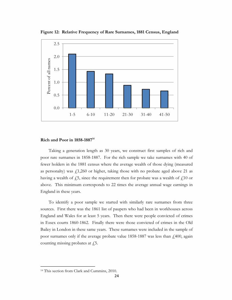
manuscript censuses of 1841-1911. Figure 12, for example, shows the share of the
population holding surnames held by 50 people or less, for each frequency grouping,
for the 1881 census of England. The vagaries of spelling and transcribing handwriting
mean that, particularly for many of the surnames in the 1-5 frequency range, this is
just a recording or transcription error. But for names in the frequency ranges 6-50
most will be genuine rare surnames. Thus in England in 1881 5 percent of the
population, 1.3 million people, held 92,000 such rare surnames. Such rare surnames
arose in various ways: immigration of foreigners to England, such as the Huguenots
after 1685 (example, “Bazalgette”), spelling mutations from more common surnames
(example, “Bisshopp”), or just names that were always held by very few people, such
as “Binford” or “Blacksmith.”
Through two forces – the fact that many of those with rare names were related,
and the operation of chance – the average wealth levels of those with rare surnames
will vary greatly at any time. We can thus divide people post 1600 into constructed
social and economic classes by focusing on those with rare surnames.
We can follow the economic and social success of those with rare surnames
1858-2011 using a number of sources. First probate records which give an indication
of the wealth at death of everyone in England and Wales by name.12 We can also
measure social status using the death register which allows us to calculate the age at
death of most people with rare surnames dying in England 1841-66, and of all people
1866-2008.13 Average age at death in all periods is a good index of socio-economic
status. The third source we use are the public records of address and occupation,
such as the electoral register, which become available for 1998 and later. The last
source is the records of those admitted to elite institutions such as Oxford and
Cambridge, available 1200-1998.
12 Those not probated typically have wealth at death close to 0. 13 For people dying 1841-1866 with rare names we can infer age at death for most of them from the censuses of 1841, 1851 and 1861, and the birth register 1837-1866.
24
Figure 12: Relative Frequency of Rare Surnames, 1881 Census, England
Rich and Poor in 1858-188714
Taking a generation length as 30 years, we construct first samples of rich and
poor rare surnames in 1858-1887. For the rich sample we take surnames with 40 of
fewer holders in the 1881 census where the average wealth of those dying (measured
as personalty) was £1,260 or higher, taking those with no probate aged above 21 as
having a wealth of £5, since the requirement then for probate was a wealth of £10 or
above. This minimum corresponds to 22 times the average annual wage earnings in
England in these years.
To identify a poor sample we started with similarly rare surnames from three
sources. First there was the 1861 list of paupers who had been in workhouses across
England and Wales for at least 5 years. Then there were people convicted of crimes
in Essex courts 1860-1862. Finally there were those convicted of crimes in the Old
Bailey in London in these same years. These surnames were included in the sample of
poor surnames only if the average probate value 1858-1887 was less than £400, again
counting missing probates at £5.
14 This section from Clark and Cummins, 2010.
0.0
0.5
1.0
1.5
2.0
2.5
1-5 6-10 11-20 21-30 31-40 41-50
Perc
ent o
f al
l nam
es

25
Table 3: Summary of the 1858-2009 Rare Name Sample
Period
Rich
Surnames
Rich
Probates
Rich
Deaths
Rich
Deaths
21+
Poor
Surnames
Poor
Probates
Poor
Deaths
Poor
Deaths
21+
1858-87 64 412 800 636* 294 77 3,291 1,720*
1888-1917 59 331 661 541 279 231 3,048 1,789
1918-1947 57 456 720 675 269 461 2,636 2,152
1948-77 47 428 625 615 283 921 3,177 2,966
1978-2008 51 289 523 518 273 1,116 3,503 3,431
Note: * Estimated from 1866-87 ratio of deaths 21+ to all deaths for 1858-65.
The surname database then consisted of everyone dying with these surnames in
the interval 1858-2008, 5 generations of 30 years, plus a last of 31 years, as well as
their ages at death and probate values where they were probated. Table 3 gives a
summary of the data.
Figure 13 shows the probate rates of the rich and poor surnames by decade, for
those dying 21 and older. Also shown as a measure of the general indigenous English
population are the probate rates for the surname “Brown.” The extreme difference in
probate rates narrows over time. But even by 2000-2008 probate rates for the rich
surname group are above average by at least 10%.
Figure 14 shows the average of the log value of the probates of those probated
among rich and poor by decade, as well as for the control group, the “Brown”
surname, until 1930-9. Probate values here in £ are normalized by dividing them by
the average annual wage in England in the year of probate. Thus the normalized
values are bequests expressed in multiples of the average annual wage.

26
Figure 13: Probate Rates of Rich, Poor and “Brown” samples, by decade
Figure 14: Ave Log Value of Probates, those probated, by decade
0
0.1
0.2
0.3
0.4
0.5
0.6
0.7
0.8
1850 1870 1890 1910 1930 1950 1970 1990 2010
Base
Rich
Poor
0
1
2
3
4
5
6
1850 1870 1890 1910 1930 1950 1970 1990 2010
Log
Rea
l Pro
bate
Val
ues
Base
Rich
Poor

27
Figure 15: Average Log Probate value, including those not probated, by decade
The average values for those probated among the rich approach those of the
poor surname group over time, but are still higher in 2000-7. Finally figure 5
combines the information in figures 3 and 4 to produce an estimate of the average
wealth at death of the rich and poor surname groups by decade, all normalized by
annual wages in pounds. The fact that generally only a minority of those dying aged
21 and above are probated means that we have to infer wealth at death for those not
probated to get average wealth levels. The measure we use for these inferred probates
is half the estate value at which probate was required. These minimum values for
required probate were £10 (1858-1900), £50 (1901-1930), £50-500 (1931-1974),
£1,500 (1975-1983), and £5,000 (1984-2011) (Turner, 628). Figure 15 shows that
there is clearly a process of long run convergence in wealth of the two surname
groups, and that process continues generation by generation, so that eventually there
will be complete convergence in wealth of the two groups. For the indigenous
population in England there are no permanent social classes, and all groups are
regressing to the social mean. But this process of convergence turns out to be much
slower than recent estimates of bs for income, earnings and education would suggest.
Average wealth at death in 2000-8 was still significantly higher for the group identified
as rich in 1858-1887. Indeed the average wealth of the “rich” surname group from
1858-1887 was still 4.2 times that of the “poor” surname group in 2000-8.
-3
-2
-1
0
1
2
3
1850 1870 1890 1910 1930 1950 1970 1990 2010
Ave
Log
Val
ue
Rich
Poor

28
It is also evident in figure 15 that the estimated rate of convergence will be
influenced by the need to infer the value of the missing probates. The jump upwards
in the relative average log wealth of the poor in 1900-9 is purely an artifact of the
raising of the probate cutoff value to £50 in this period, which led missing values
under our procedure to be inferred as £25, compared to £5 before. We hope to find
better ways of inferring these missing values in future work.
Another way we can observe this convergence is though average age at death.
Life expectancy in England, for example, has since at least the nineteenth century
been dependent on socio-economic status. In 2002-2005 life expectancy for
professionals in England and Wales was 82.5 years. For unskilled manual workers it
was only 75.4. Thus another way to observe whether the rich and poor of 1858
converge, and how quickly, is using the death register for England and Wales, which
for 1866-2005 shows the age of death of everyone in England by name.
If we take just the overall average age of death by group then the differences in
1857-1887 are dramatic: 50.7 for the rich, 31.7 for the poor. As figure 16 shows these
average ages at death converged steadily over time, but had not completely converged
by 1978-2008. Average age at death for the rich surnames was still 78.0 for the rich
surnames, compared to 74.1 for the poor, a difference of 3.9 years. The reason for
the extreme difference in life expectancy in the first generation is actually a
combination of lower death rates for the rich at each age, but also differences in
fertility which expose more of the poor population in the early years to high child
mortality risks.
Since we do not know the age structure of the population, measuring fertility
accurately is not possible. However, given the average age at death of those 21+ we
can estimate for each group in each decade the stock of the population in the 25-45
age group if we assume (counterfactually) a uniform age distribution. Then we can
calculate a rough measure of the numbers of children born per woman. This is
shown in figure 17.
As can be seen there are substantial differences in the estimated fertility of rich
and poor surname groups which while narrowing over time are still present in 2000-8.
In the nineteenth century the higher fertility of the poor was partially counterbalanced
by substantially higher infant and child mortality. Thus child mortality in the poor

29
Figure 16: Average Age at Death, by Generation
Figure 17: Estimated births per woman by decade, rich and poor surnames
Note: By construction this will overestimate fertility in a stable population since the 25-45 cohort will be larger than is estimated here.
0
10
20
30
40
50
60
70
80
0 1 2 3 4
Ave
rage
Age
at D
eath
Generation
Rich
Poor
0
2
4
6
8
1850 1870 1890 1910 1930 1950 1970 1990 2010
Birt
hs p
er w
oman
Rich
Poor

30
Figure 18: Numbers of Poor 21+ Relative to the Rich, 1858-2009
group before 1900 was 138 per 1000 more than for the rich. But the relative
population of the poor surname group has increased substantially over time relative to
that of the rich group. To measure the population of those aged 21+ in each group
we used the formula
21
where the average age of death is that of those dying 21+. Figure 18 shows the
relative size of the stock of “poor” surname people, and the stock of “brown”
surname people, compared to the stock of the “rich” surname group. The relative
poor stock rose more than 150 percent between 1858-87 and 1978-2008. But the
brown stock increased even more, by 200 percent.
Thus in this period, instead of survival of the richest, and the growing share of
0.0
0.5
1.0
1.5
2.0
2.5
3.0
3.5
0 1 2 3 4
Stoc
k of
rich
and
poo
r 21+
Generation
Poor/Rich
Brown/Rich

31
the rich descendants in population, we see the decline of the rich class even as it
regresses towards the social mean. It must be emphasized that these stock estimates
are subject to much error, but they are underlain by a basic fact that the numbers of
those dying with rare rich surnames declined substantially relative to those with rare
poor surnames, and even more substantially relative to a common name like Brown.
Estimating bs
We can estimate the bs, the measure of persistence in wealth, in several different
ways. If we define yRi and yPi as the average of ln wealth for generation i for the rich
and poor surname groups, then the b linking this generation with the nth future
generation can be measured simply as
yRi+n - yPi+n = b(yRi - yPi) This estimation has an advantage that after the first generation, when rich and poor
samples were chosen partly based on wealth, there is no tendency for the b estimate
to be attenuated by measurement error in wealth, since the average measurement
error for both rich and poor groups will be zero. Also as long as wealth is linked to
true underlying social status, even imperfectly, this measure will show how rapidly the
two groups are moving towards each other. However, there is a disadvantage that
there is no associated standard error with the estimated b. Figure 9 shows the mean
log wealth of each group by generation, and table 3 the implied bs.
Another advantage of this estimate is that by construction,
b04 = b01.b12.b23.b34
so the individual period b estimates are consistent with the observed long run
mobility.
It is striking how high the b estimates are in table 4. It is also striking that over 4
generations the b is still 0.26, though as figure 19 shows there will be eventual
convergence in wealth. The fact that the b between generations 3 and 4 was only 0.53
might give some hope of faster regression to the mean in future. But if you look at
figure 15, you will see that for those dying in 2000-8 there is no sign of any faster
convergence, though this may just be random error. Wealth at death now may be

32
much more subject decade to decade to the vagaries of the housing market and stock
market.
Suppose we count complete regression to the mean as the two groups of
descendants having average wealth within 10 percent. If we assume the b from now
on is the one between the last two generations of 0.53, it will take 8 generations (the
generation of 2098-2127) to achieve this. But if the future b is the average of the
between generations bs for 1858-2008, then complete convergence will require 12
generations (2218-2247).
The more conventional way to estimate b is by taking the average wealth of each
surname in each generation as the unit of observation, and then estimate by OLS the
b values (weighting by the average number of observations in each surname group).
The regressions run are
(4)
where here yn+i is the average log wealth by surname in period i+n. As noted this
measure is always subject to attenuation bias because of the errors in measuring
wealth, and the imperfect link between wealth and true underlying social status. The
first set of regression coefficients are reported in table 5, along with standard errors.
We included controls for the fraction of testators in each surname group who were
female in each generation.

33
Figure 19: Average Log Probate value, by generation
Table 4: Wealth Persistence measures
Generation
1
Generation
2
Generation
3
Generation
4
Generation 0
0.74
0.64
0.48
0.26
Generation 1
0.87
0.65
0.35
Generation 2
0.75
0.40
Generation 3
0.53
-3
-2
-1
0
1
2
0 1 2 3 4
Ave
rage
ln W
ealth
(All)
Generation
Rich
Poor

34
Table 5: Estimated b values between generations, conventional estimates
Generation
1
Generation
2
Generation
3
Generation
4
Generation 0
0.662 (.030)
0.604 (.027)
0.469 (.028)
0.308 (.032)
Generation 1
0.748 (.034)
0.567 (.035)
0.379 (.041)
Generation 2
0.684 (.034)
0.441 (.041)
Generation 3
0.501
(0.044)
Note: Standard errors in parentheses.
As predicted the one-period b estimates here are always lower than with the
estimates in table 4, though not dramatically so. However, we do see evidence in
table 4 that the b’s either are being estimated as too low, or the rich and poor groups
are regressing to different means. For if the process was the Markov one that most
studies of social mobility assume, then
b04 = b01.b12.b23.b34
In fact we see in table 4 that
= 0.31 > . . . = 0.67×.75×.68×.50 = 0.17
The long run regression to the mean is slower than the one period bs would
predict. One possibility is that measurement error in wealth is leading to b estimates
that are too low. If there is the same measurement error in estimating the bs, an
attenuation factor θ, between any two generations, then

35
= b04θ > . . . = . . . = θ4
In this case we can get better estimates of the true bs between periods by taking
the ratios of the estimated bs. Thus
This method suggests the following “true” values of b across each generation of
b01 = 0.89, b12 = 0.83, b23 = 0.88, b34 = 0.66.
Another possibility, however, is that the rich and poor surname groups are
regressing to different means, so that they will never converge. To test for this
possibility we estimate (4), but with a separate intercept term for the rich surnames.
Table 6 shows the results of this estimation. Now the b estimates fall very
substantially, and at the same time the rich are estimated across all generations to be
regressing to a higher mean than that of the poor (DRICH, the indicator for the rich
surnames, is positive). If we were just to estimate wealth mobility across two
generations with this method we would conclude that rich and poor would never
converge.
However, while DRICH is always positive and significant, it is clear from figure
19, and from the associated evidence on measures such as average years lived, that the
rich and poor surnames groups will eventually converge. And in table 6 we see that
the separate intercept term for the rich surname group is always declining in size as we
go across more generations. This suggests that Hertz’s finding that Jews and Blacks
in the US were regressing to means different from the general population in the long
run may be just an artifact of the estimation method, and that instead there is a much
slower general regression to the same social mean (Hertz, 2005).
All this suggests that there is no substitute for observing the long run outcomes
in trying to observe the process of social mobility. Regressions run on the
characteristics of just two adjacent generations will not be able to statistically predict
the nature and the rate of the long run mobility regime. Our conclusion here is that
while the bs were high, very high, there is no sign that the upper class will persist in
advantage for ever, or the lower class persist in disadvantage.

36
Table 6: Intergenerational b, Distinct Intercepts for Rich and Poor
Generation
1
Generation
2
Generation
3
Generation
4
Generation 0.360 0.450 0.246 0.147
0 (.072)
(.065) (.068) (.075)
Generation 0.429 0.331 0.195 1 (.057)
(.057) (.064)
Generation 0.472 0.320 3 (.055)
(.065)
Generation 0.398 4 (.058)
DRICH 1.663 0.861 1.074 0.680 0 (.329) (.303) (.317)
(.342)
DRICH 1.184 0.963 0.783 1 (.213) (.215)
(.239)
DRICH 0.809 0.514 2 (.182)
(.216)
DRICH 0.467 3 (.172)

37
Will Universal Regression to the Mean Continue in England?
What the rare surname dataset implies is somewhat paradoxical. On the one
hand the Beckerian vision of ultimate regression to the social mean seems to apply to
modern England as well as late medieval England. In the long run no social class, at
least among the indigenous English and immigrants from western Europe, is able to
stop from regressing to the mean. The poor similarly regress upwards. There are no
permanent upper classes and under classes, but instead long run equality. On the
other hand these processes are occurring at a very slow pace, as slow as in medieval
England.
There is evidence, however, that England’s period of complete social mobility
will potentially end as a result of the immigration in the last 100-200 years of new
groups to England who are more heterogenous in terms of religion and ethnicity.
Table 7 thus shows the median wealth of families from a variety of religious and
ethnic backgrounds in England in 2006/8. This snapshot of wealth in one cross
section does not reveal the underlying dynamics of wealth in England. But it does
suggest that these new immigrant groups are experiencing radically different social
situations in England, with Jews and Bangladeshi’s forming groups at the polar
opposite. Given the rates of convergence to the mean we observe for the indigenous
population, even if we assume these rates of regression would apply to these
immigrant groups, it would take 6-10 generations for Bangladeshi and Jewish median
wealth to equalize. But more likely there are characteristics of these groups that
would imply even slower rates of convergence, implying that for England in the next
200-300 years there will be quite clear and identifiable persistent upper and lower
classes, not observed since the times of the Norman Conquest to 1460.

38
Table 7: Total wealth inequality between groups in Britain, 2006/08
Religion/Ethnicity
Median wealth (£)
Jewish 422,100 Sikh 228,700 Christian 222,900 Hindu 206,100 Other Religion 161,100 No religion 138,500 Buddhist 74,800 Muslim 41,600 Pakistani 96,900 Black Caribbean 75,500 Black African 20,600 Bangladeshi 15,000 ALL 204,500 Source: Wealth and Assets Survey 2006/08.
Conclusions
What should we think of these results? Does it imply a society of enduring
privilege, with limited opportunities for the lower class? Assuming the b estimates
here survive greater amounts of data, the problem is that we have no clear idea of
what b would be in a society of complete opportunity and access. Indeed Richard
Herrnstein and Charles Murray in The Bell Curve argue that recent creation of a
meritocracy, combined with assortative mating, will lead to an ever more stratified
society, but stratified by intellectual abilities that are strongly inherited (Herrnstein and
Murray, 1996).
It is also likely that most of the strong correlation of wealth across generations
does not come from direct transfers of assets from parents to children. In other work
Clark has shown that only about a third of the correlation of wealth between fathers

39
and sons in England 1550-1850 is explained by bequests from fathers (Clark, 2007).
Rich fathers have rich sons mainly because the sons are inheriting other characteristics
of the fathers, such as their genetics, which are transmitted independently of how
many surviving children father’s have at death.
The fact that by 2000-8 there was still a difference in average age at death
between the rich and poor surname groups does suggest that other types of
transmission of characteristics that create socio-economic advantage, social and
genetic, are important. Years lived is not going to be directly a function of wealth, but
much more a function of lifestyle, aptitudes, and attitudes. There is no expectation
that in England, with its open access National Health Service, wealth would create
much direct benefit in terms of years lived. Wealth must thus just be correlated with
other attributes that promote longer lives. So the plausible cause of the
intergenerational correlation of wealth is not inheritance of wealth, but of these other
attributes.
It matters to people’s sense of the fairness of society whether the high correlation
of wealth across generations is largely the product of home environment, or of
genetics. The bs we find here for wealth are equivalent in magnitude to those for the
most strongly inherited genetically controlled human traits. The b for human height
for example between parents and children in modern high income societies is 0.8-0.9,
with most of this from genetics and not environment (height differences by social
class are now modest). But we see nothing problematic in this high height b, since it
is mainly genetic. So what matters in our attitude to the bs found here is whether they
turn out to be largely explained by genetics. Twin studies reveal that both earnings
and education are strongly influenced by genetics, but there is no equivalent study for
wealth.
We also have to do more in looking at the startling divergence in the numbers of
those with the rich rare surnames compared to those with poor rare surnames and the
indigenous population (represented by the name Brown). Our data suggests that
starting with the generation born around 1860, the poor and the general population
had much greater reproductive success than our rich group, resulting in much larger
numbers of poor deaths in the generations 3 and 4. Indeed at a time when English
population tripled, the rich surname group barely increased its numbers. This might,
however, in part arise from greater migration of the rich from England to the USA, to
the British Empire, and to Europe in the late nineteenth century. And indeed there is

40
evidence in the probates that a significant number of the rich were dying abroad. If
the wealthy are in general more cosmopolitan and polyglot, so that they end up spread
around the globe, then this would explain their surprisingly small numbers in later
years.
But the crude estimates of fertility shown in Figure 17 control for out migration,
in that it looks at deaths in England compared to births in England. And these
suggest consistently low fertility rates by the rich surname group, though again with a
tendency to converge on the poor. This, however, does mean that while all wealth is
ultimately transitory, and there is no enduring ruling class, the ruling group of any
moment in the modern world is likely to see a permanent reduction in their share of
the population. Wealth does have persistent effects, but only through demography.
Since some of the rich surnames were distinctive and aristocratic in their sound,
could it be that as people in this group moved down they changed surname? The
names in our rich sample include Willoughby de Broke, Bazalgette, Du Cane, and
Champion de Crespigny. With a larger sample of rich surnames we will be able to
check if the relative frequency of such aristocratic surnames declined over time, as a
possible indicator of name changing. However, these four names were 6.6 percent of
rich surname deaths in 1858-87, and 6.1 percent of deaths in 1978-2008. So there is
no indication so far that elite names are being abandoned as people become less elite.
One interesting issue that this raises, however, is with the quality-quantity
tradeoff theory that dominates modern discussions of fertility. The rich had fewer
children, yet in the end they were condemned to regress to the social mean. The poor
had many children yet moved up to the social mean. So interestingly there was no
strategy of investing more in fewer children that could keep the elite in the same
social position permanently. The forces of regression are stronger than any family
strategies could overcome. In that sense though regression to the mean is slow here,
its inexorable power on elites and under classes is surprising in light of the ability of
elites to trade off quantity for quality in children, and to endow their children with
considerable wealth.

41
Data Sources
UK, House of Commons Papers. 1861. Paupers in workhouses. Returns from each
workhouse in England and Wales, of the name of every adult pauper who has been an inmate of the workhouse during a continuous period of five years. Vol LV, 201. Cmd. 490.
Emden, Alfred B. 1957. A Biographical Register of the University of Oxford to AD 1500 (3 vols.). Oxford: Clarendon Press.
Emden, Alfred B. 1974. A Biographical Register of the University of Oxford AD 1501 to 1540. Oxford: Clarendon Press.
England and Wales, Census, 1851-1881. Available online at http://www.nationalarchives.gov.uk/records/census-records.htm
England and Wales, Index to Wills and Administrations, 1858-2011. Principle Probate registry, London (available online 1861-1942 at Ancestry.co.uk).
England and Wales, Register of Births, 1837-2005. Available online at Ancestry.co.uk. England and Wales, Register of Deaths, 1837-2005. Available online at Ancestry.co.uk. England and Wales, Register of Deaths, 2006-2010. London Metropolitan Archives. The Proceedings of the Old Bailey, 1674-1913. http://www.oldbaileyonline.org/index.jsp Index to the Prerogatory Court of Canterbury Wills, 1384-1858. (UK National Archives,
London). Keats-Rohan, K. S. B. 1999. Domesday People: A Prosopography of Persons Occurring in
English Documents 1066-1166. Woodbridge, Suffolk: The Boydell Press. Public Record Office. 1904. Calendar of Inquisitions Post Mortem and other Analogous
Documents preserved in the Public Record Office, Vol. 1 Henry III. London: Public Record Office.
Public Record Office. 1906. Calendar of Inquisitions Post Mortem and other Analogous Documents preserved in the Public Record Office, Vol. 2 Edward I. London: Public Record Office.
References Becker, Gary. 1988. “Family Economics and Macro Behavior.” American Economic
Review, 78: 1-13. Becker, Gary and Nigel Tomes. 1986. “Human Capital and the Rise and Fall of
Families.” Journal of Labor Economics, 4(3): S1-S39. Biblarz, Timothy J., Vern L. Bengtson and Alexander Bucur. 1996. “Social Mobility
Across Three Generations.” Journal of Marriage and the Family, 58(1): 188-200. Black, Sandra E. and Paul J. Devereux. “Recent Developments in Intergenerational
Mobility.” Working Papers, Geary Institute, University College Dublin. 2010. Bowles, S. and H. Gintis. 2002. “The Inheritance of Inequality” Journal of Economic
Perspectives. Volume 16, Number 3, 1 August 2002, pp. 3-30(28) Clark, Gregory. 2007. A Farewell to Alms: A Brief Economic History of the World.
Princeton: Princeton University Press. Clark, Gregory and Neil Cummins. 2010. “Was there ever a Ruling Class? Rare
Surnames and Long Run Social Mobility in England, 1858-2011?” Working Paper, Cliometrics Society Conference, Boulder, Colorado.

42
Galton, Francis 1869. Hereditary Genius: An Enquiry into its Laws and Consequences.
London: Macmillan and Co. Galton, Francis. 1877. “Typical laws of heredity.” Proceedings of the Royal Institution 8:
282-301 Galton, Francis 1886. "Regression Towards Mediocrity in Hereditary Stature".
Journal of the Anthropological Institute of Great Britain, 15: 246–263. Güell, Maia, José V. Rodríguez Mora, and Telmer, Chris. 2007. “Intergenerational
Mobility and the Informative Content of Surnames.” Working Paper, Edinburgh University.
Harbury, C. D. and Hitchens, D. M. W. N. 1979. Inheritance and Wealth Inequality in Britain. London: Allen and Unwin.
Herrnstein, Richard J. and Charles Murray. 1996. The Bell Curve: Intelligence and Class Structure in American Life. New York: Free Press.
Hertz, Thomas. 2005. “Rags, Riches and Race: The Intergenerational Mobility of Black and White Families in the United States” in Samuel Bowles, Herbert Gintis and Melissa Osborne (eds.), Unequal Chances: Family Background and Economic Success, 165-191. New York: Russell Sage and Princeton University Press.
Jebb, Richard. 1858. The act to amend the law relating to probates and letters of administration in England. London: V. & R. Stevens and G.S. Norton, H. Sweet, and W. Maxwell.
Jobling, Mark A. 2001. “In the name of the father: surnames and genetics.” TRENDS in Genetics, Vol. 17, No. 6 (June): 353-357.
King, Turi E., Stéphane J. Ballereau, Kevin E. Schürer, and Mark A. Jobling. 2006. “Genetic Signatures of Coancestry within Surnames.” Current Biology, 16 (21 February): 384-388.
Long, Jason and Joseph Ferrie. 2009. “Intergenerational Occupational Mobility in Britain and the U.S. since 1850.” Working Paper, Colby College, Maine.
Mayer, Susan E. and Leonard M. Lopoo. 2005. “Has the Intergenerational Transmission of Economic Status Changed.” Journal of Human Resources, 40(1): 169-185.
Mazumdar, Bhaskar. 2005. “Fortunate Sons: New Estimates of Intergenerational Mobility in the United States Using Social Security Earnings Data.” Review of Economics and Statistics, 87(2): 235-255.
McCauliff , C.M.A. 1986. “The First English Adoption Law and its American Precursors.” Seton Hall L. Rev: 16:656-677
Nimubona, Alain-Désiré and Désiré Vencatachellum. 2007. “Intergenerational Education Mobility of black and white South Africans.” Journal of Population Economics, 20(1): 149-182.
Solon, Gary. 1999. "Intergenerational mobility in the labor market," in Handbook of Labor Economics, Vol. 3A, Orley C. Ashenfelter and David Card (eds.), Amsterdam: Elsevier.
Solon, Gary. 2002. "Cross Country Differences in Intergenerational Earnings Mobility," Journal of Economic Perspectives, 16(3): 59-66.
Turner, John D. 2010. “Wealth concentration in the European periphery: Ireland, 1858–2001.” Oxford Economic Papers, 62: 625-646.
Watson, H. W. and Francis Galton. 1875. "On the Probability of the Extinction of Families", Journal of the Anthropological Institute of Great Britain, 4: 138–144.

43