Warming Trend of the Indian Ocean SST and Indian Ocean Dipole from 1880 to 2004*

CHIE IHARA, YOCHANAN KUSHNIR, AND MARK A. CANE

Lamont-Doherty Earth Observatory, Columbia University, Palisades, New York

(Manuscript received 9 March 2007, in final form 14 September 2007)

ABSTRACT

The state of the Indian Ocean dipole representing the SST anomaly difference between the western andsoutheastern regions of the ocean is investigated using historical SST reconstructions from 1880 to 2004.First, the western and eastern poles of the SST-based dipole mode index are analyzed separately. Both thewestern and eastern poles display warming trends over this period, particularly after the 1950s. The westernpole tends to be anomalously colder than the eastern pole from 1880 to 1919, whereas in the interval1950–2004 the SST anomalies over the western pole are comparable to those over the eastern pole thoughthere are occasional outliers where the eastern pole is anomalously colder than the western pole.

The tendencies of the occurrences of positive and negative dipole events in September–November showthree distinct regimes during the period analyzed. In 1880–1919, negative dipole events associated with LaNiña events occur more frequently than positive events. In 1920–49, some weak positive events occurrelatively independently of El Niño events over the Pacific. The period of 1960–2004 is characterized bystrong and frequent occurrences of positive events associated with El Niño events.

1. Introduction

Though there had been earlier studies of the inter-annual variability of the zonal sea surface temperature(SST) gradient over the equatorial Indian Ocean (e.g.,Saha 1970; Reverdin et al. 1986), after Saji et al. (1999)and Webster et al. (1999) discovered a phenomenonthat includes both atmospheric and oceanic variablesand called it the Indian Ocean dipole mode or IndianOcean zonal mode, the number of studies related to thisphenomenon increased dramatically. According to Sajiet al. (1999), the Indian Ocean dipole mode is charac-terized by the anomalous west–east SST gradient ac-companying zonal wind anomalies over the equatorialIndian Ocean; during positive events the western In-dian Ocean is warmer than normal; the southeast In-dian Ocean, off of Sumatra, is colder than normal; andthe anomalous easterlies appear around the centralequatorial Indian Ocean. They also found that the di-

pole events were seasonally phase locked: an eventstarted in May–June, matured in October, and decayedin boreal winter. Li et al. (2003) suggested that a ther-modynamic air–sea interaction over the southeast In-dian Ocean explained this feature of the dipole mode.In boreal summer, the anomalous wind induced by thecooling over this region enhances the mean southeast-erly flow over the equatorial Indian Ocean, which inturn enhances the surface evaporation, vertical mixing,and coastal upwelling off of Sumatra. This sequence offactors further cools the southeast Indian Ocean. Whenthe mean flow changes from southeasterly to north-westerly in boreal winter, the same anomalous flowweakens the mean flow and dampens the cooling overthe southeast Indian Ocean. The thermodynamic air–sea interaction works as a positive feedback in borealsummer but also as a negative feedback in boreal win-ter. Thus, Li et al. (2003) claimed that feedback mecha-nisms that were dependent on the season could explainwhy dipole events developed in boreal summer and de-cayed in boreal winter.

There is some controversy over whether the dipolemode events are independent of El Niño–Southern Os-cillation (ENSO) and are inherent to the Indian Ocean(Allan et al. 2001). Saji et al. (1999) and Webster et al.(1999) claimed that the events could occur withoutENSO, pointing to 1961, a year when a strong positive

* Lamont-Doherty Earth Observatory Contribution Number7107.

Corresponding author address: Chie Ihara, Lamont-DohertyEarth Observatory, Columbia University, 61 Route 9W, Pali-sades, NY 10964-8000.E-mail: cihara@ldeo.columbia.edu

15 MAY 2008 I H A R A E T A L . 2035

DOI: 10.1175/2007JCLI1945.1

© 2008 American Meteorological Society

JCLI1945

dipole event occurred without El Niño. Lau and Nath(2004) suggested that in addition to ENSO, the south-ern annular mode (SAM) could be one of the triggersof the Indian Ocean events based on output from acoupled general circulation model simulation. Fischeret al. (2004) concurred with the findings of Lau andNath and in their study, the cold SST in the southeasttropical Indian Ocean accompanying the strong Mas-carene high triggered the northward penetration of thesoutheast trades over the equatorial Indian Ocean,which was favorable for the development of the dipolemode.

As a mode of climate variability in the Indian Ocean,the impacts of the Indian Ocean dipole on the globalclimate are also examined. Previous papers have ad-dressed the connection of the dipole mode to the cli-mate of India (Ashok et al. 2001, 2004b; Ihara et al.2008), East Africa (Clark et al. 2003; Behera et al.2005), the extratropics (Guan and Yamagata 2003; Sajiand Yamagata 2003), and the East Asian monsoon(Kripalani et al. 2005). Discussions of the definition andphysical mechanisms of the Indian Ocean dipole mode,particularly its relation to ENSO, are on going. How-ever, it may now be fair to say that its existence andscientific importance are becoming accepted within thescientific community.

The Indian Ocean dipole, defined by a zonal SSTgradient, is known to have decadal to multidecadalvariability (e.g., Annamalai et al. 2005; Ashok et al.2004a; Chang et al. 2006; Kripalani and Kumar 2004;Tozuka et al. 2007). Annamalai et al. (2005) suggesteda connection between the strong dipole events in the1960s and 1990s and the Pacific decadal variability.Ashok et al. (2004a) demonstrated the existence of8–25-yr low-frequency signals of the Indian Ocean di-pole. Tozuka et al. (2007) pointed out asymmetric oc-currences of positive and negative dipole mode eventsover a period that spanned about 10 yr and called it thedecadal modulation of interannual Indian Ocean dipolemode events. In terms of multidecadal variability, Kri-palani and Kumar (2004) found that the Indian Oceandipole was in a negative phase in the period between1880 and 1920 and was in a positive phase in the periodbetween 1960 and 2000. Our interest here is in the mul-tidecadal variability, as found in Kripalani and Kumar(2004), that is, irregular occurrences of negative (in thelate nineteenth century and the early twentieth cen-tury) and positive events (in the second half of thetwentieth century). Thus, the time scale of the changefocused upon in this study is about a century—longerthan earlier studies on decadal variations.

We are particularly interested in multidecadal vari-ability since this secular change in the occurrences of

positive and negative events between the first and sec-ond halves of the twentieth century is conceivably re-lated to the warming trend over the Indian Ocean dur-ing this period. The warming SST over the IndianOcean has been addressed by many earlier papers (Al-lan et al. 1995; Terray and Dominiak 2005, and refer-ences therein). Allan et al. (1995) examined the condi-tions of the Indian Ocean from 1900 to 1983 in borealwinter and found that overall, the SST displayed awarming trend. Terray and Dominiak (2005) showedthat the entire Indian Ocean basin demonstrated sub-stantial warming after the 1976–77 climate regime shiftover the Pacific Ocean. These changes may in part benatural variation, or may be the local manifestation ofglobal warming caused by the anthropogenic green-house gases and aerosols. If we suppose these warmingtrends are homogeneous in space, the anomalous SSTgradient over the equatorial Indian Ocean should re-main the same. But if not, these trends could affect thestrength of both positive and negative dipole events,and may be related to the multidecadal variability ofthe Indian Ocean dipole mode events. Thus, it is ofgreat importance to delineate the relationship betweenthe SST anomalies in the western and eastern poles ofthe dipole mode over the long term in consideration ofthe warming trend over these regions.

In this paper, we investigate the state of the IndianOcean dipole as represented by SST anomalies from1880 to 2004, and reveal that a change occurred in therelationship between SST anomalies over the westernand eastern poles of the Indian Ocean dipole. Thechange in the characteristics of the same positive andnegative dipole events defined by their index is alsodelineated during this long-term period. Since the weakwarming trend in the early half of the twentieth centurycompared to the intense warming after the mid-1970s isreported in the global mean annual land surface airtemperature (e.g., Jones et al. 2006), we infer thatwarming trend of the Indian Ocean from 1880 to 2004may not be monotonic and thus we try to take intoaccount the different regimes of the warming trend inour analysis. Our work is different from that of Ashoket al. (2003) in that they examined the long-term stateof the Indian Ocean dipole because the trend of thedipole mode index was linearly removed in their analy-sis. Kripalani and Kumar (2004) pointed out the multi-decadal variability of the Indian Ocean dipole but thestate of the Indian Ocean dipole in the warming trend,particularly the relationship between the western andeastern poles, was not fully examined there. Section 2 isdevoted to the description of the datasets used in thisstudy. In section 3, we discuss the warming trends overthe western and eastern poles separately and present

2036 J O U R N A L O F C L I M A T E VOLUME 21

their relationships in three different periods. In section4, we demonstrate the changes within the occurrencesof positive and negative events and the Indo-PacificSST patterns associated with these events. Section 5 isdevoted to a summary and discussions.

2. Data descriptions

Monthly, 1° � 1° gridded SST anomalies from 1880to 2004 are obtained from Smith and Reynolds (2004),the so-called National Oceanic and Atmospheric Ad-ministration/National Climatic Data Center (NOAA/NCDC) Extended Reconstructed SST (ERSST) data-set, version 2. For comparison, monthly 4° � 4° griddedSST anomalies from 1880 to 2004 obtained from Kap-lan et al. (2003) are also used. SST anomaly data areaveraged over 3 months by season: December–Febru-ary, March–May, June–August, and September–No-vember. The climatology in this study is defined as themean SST during the period between 1880 and 2004 toaddress the state of the Indian Ocean SST, includingthe trend component.

Different methods are used for the reconstructions ofthe ERSST and Kaplan SST datasets. Smith and Reyn-olds (2003) separated low- and high-frequency vari-abilities and reconstructed the high-frequency variabil-ity by the projection method. Kaplan et al. (2003) usedan optimal smoothing method assuming the stationarityof the data in the modern base period and dealt with allfrequencies in the same manner. Thus, there is a criti-cism that the warming trend of SST over the twentiethcentury is underestimated in the Kaplan SST data whileit more effectively captures the large-scale structures ofSSTs (Hurrell and Trenberth 1999). However, the re-sults we are going to show do not differ remarkablybetween the ERSST data and the Kaplan SSTs eventhough some discrepancies are expected between thesetwo SST datasets.

The data prior to the 1880s are not included in ourstudy to avoid the uncertainties that have been re-ported to affect this early period (Kaplan et al. 1998;Smith and Reynolds 2003). The equatorial IndianOcean displays rich data coverage from the early periodof analysis compared to the equatorial eastern Pacific.The Comprehensive Ocean–Atmosphere Data Set(COADS) SSTs, from which the ERSST results arederived (Slutz et al. 1985), show that, roughly speaking,the tropical Indian Ocean has twice the number of ob-servations as the equatorial eastern Pacific from thelate nineteenth century throughout the 1960s, exceptfor the 1940s when the data coverage was sparse in theboth oceans. Thus, it can be said that the tropical IndianOcean is the region that offers reliable SST datasets

even in the late nineteenth century and the early twen-tieth century. There may be a concern about the dataquality before the 1950s compared to the data qualityafter the 1950s in the tropical Indian Ocean, but thenumber of observations in the equatorial Indian Oceanbefore the 1950s is comparable or sometimes larger tothat from the 1950s throughout the 1970s, except forthree short periods: 1880–1900, just before 1920, andthe time of World War II, 1940–45. In 1880–1900, thenumber of observations of the tropical Indian Ocean isgenerally about half of that from the 1950s throughoutthe 1970s. But in the short periods just before 1920and 1940–45, the number of observations of the tropi-cal Indian Ocean drops steeply compared to the pre-ceding period. The overall tendency of the data cover-age is almost the same for the data from version 5 ofthe Met Office Historical Sea Surface Temperature(MOHSST5) dataset, from which the Kaplan SST dataare derived (Kaplan et al. 1998). We judge that thoughthe SST data before the 1950s are not as good as theSST data from the 1950s throughout the 1970s becauseof these short data-sparse periods, we still believe thatthe historical SST datasets in the early period are reli-able enough to conduct research on the secular changeof the equatorial Indian Ocean SST. We use cautionwith the results based on the data-sparse periods men-tioned above and we compensate for the limitations ofthe data quality during these periods; thus, we confirmour results by using the two new and different SSTreconstructions.

3. Western and eastern poles of the Indian Oceandipole events

a. Trends in the SST anomalies over the westernand eastern poles

The Indian Ocean dipole events are represented bythe dipole mode index obtained by the SST anomalydifference over the western Indian Ocean and thesoutheast Indian Ocean (hereafter referred to asSSTDMI). The western pole of SSTDMI is located atthe western equatorial Indian Ocean (hereafter re-ferred to as WEIO) representing SST anomalies aver-aged in the box from 10°S to 10°N and from 50° to 70°E(Fig. 1). The eastern pole of SSTDMI is located at theeastern equatorial Indian Ocean (hereafter referred toas EEIO) representing SST anomalies averaged in thebox from 10°S to 0° and from 90° to 110°E (Fig. 1).Figure 2 shows the 10-yr running means of the seasonalWEIO and EEIO from 1880 to 2004; the top panelcorresponds to WEIO and EEIO obtained from theERSST data, and the bottom panel corresponds to theresults obtained from the Kaplan SST data. Both the

15 MAY 2008 I H A R A E T A L . 2037

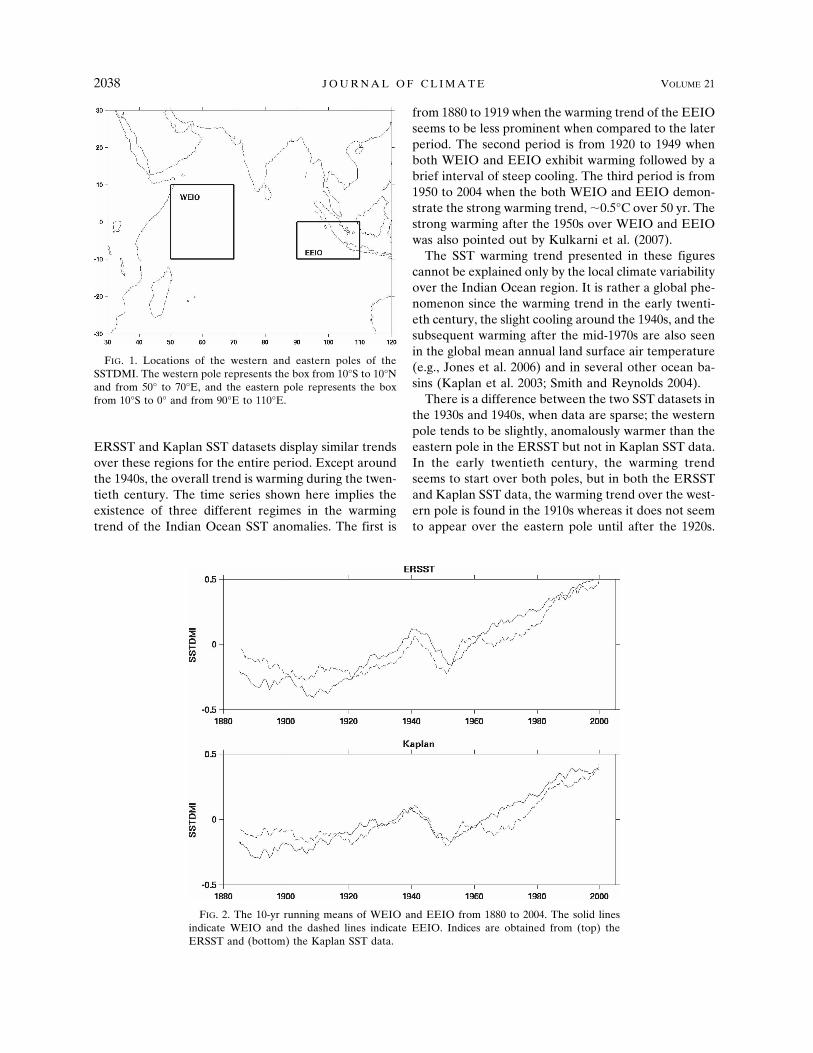
ERSST and Kaplan SST datasets display similar trendsover these regions for the entire period. Except aroundthe 1940s, the overall trend is warming during the twen-tieth century. The time series shown here implies theexistence of three different regimes in the warmingtrend of the Indian Ocean SST anomalies. The first is

from 1880 to 1919 when the warming trend of the EEIOseems to be less prominent when compared to the laterperiod. The second period is from 1920 to 1949 whenboth WEIO and EEIO exhibit warming followed by abrief interval of steep cooling. The third period is from1950 to 2004 when the both WEIO and EEIO demon-strate the strong warming trend, �0.5°C over 50 yr. Thestrong warming after the 1950s over WEIO and EEIOwas also pointed out by Kulkarni et al. (2007).

The SST warming trend presented in these figurescannot be explained only by the local climate variabilityover the Indian Ocean region. It is rather a global phe-nomenon since the warming trend in the early twenti-eth century, the slight cooling around the 1940s, and thesubsequent warming after the mid-1970s are also seenin the global mean annual land surface air temperature(e.g., Jones et al. 2006) and in several other ocean ba-sins (Kaplan et al. 2003; Smith and Reynolds 2004).

There is a difference between the two SST datasets inthe 1930s and 1940s, when data are sparse; the westernpole tends to be slightly, anomalously warmer than theeastern pole in the ERSST but not in Kaplan SST data.In the early twentieth century, the warming trendseems to start over both poles, but in both the ERSSTand Kaplan SST data, the warming trend over the west-ern pole is found in the 1910s whereas it does not seemto appear over the eastern pole until after the 1920s.

FIG. 2. The 10-yr running means of WEIO and EEIO from 1880 to 2004. The solid linesindicate WEIO and the dashed lines indicate EEIO. Indices are obtained from (top) theERSST and (bottom) the Kaplan SST data.

FIG. 1. Locations of the western and eastern poles of theSSTDMI. The western pole represents the box from 10°S to 10°Nand from 50° to 70°E, and the eastern pole represents the boxfrom 10°S to 0° and from 90°E to 110°E.

2038 J O U R N A L O F C L I M A T E VOLUME 21

Over the equatorial Indian Ocean, the annual meanwinds are weak westerlies and the thermocline depth isrelatively flat but larger in the east than in the west (Liet al. 2003). Thus, it is possible to hypothesize that itmight take a longer time to warm the upper layer of theeastern equatorial Indian Ocean than the western equa-torial Indian Ocean. Also, since WEIO extends farthernorthward as compared to EEIO, the difference in thetiming may arise from the north–south gradient of thewarming trend.

b. Relationships between WEIO and EEIO in threeperiods

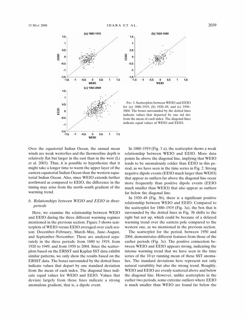
Here, we examine the relationship between WEIOand EEIO during the three different warming regimesmentioned in the previous section. Figure 3 shows scat-terplots of WEIO versus EEIO averaged over each sea-son: December–February, March–May, June–August,and September–November. These are analyzed sepa-rately in the three periods: from 1880 to 1919, from1920 to 1949, and from 1950 to 2004. Since the scatter-plots based on the ERSST and Kaplan SST data exhibitsimilar patterns, we only show the results based on theERSST data. The boxes surrounded by the dotted linesindicate values that depart by one standard deviationfrom the mean of each index. The diagonal lines indi-cate equal values for WEIO and EEIO. Values thatdeviate largely from those lines indicate a stronganomalous gradient, that is, a dipole event.

In 1880–1919 (Fig. 3 a), the scatterplot shows a weakrelationship between WEIO and EEIO. More datapoints lie above the diagonal line, implying that WEIOtends to be anomalously colder than EEIO in this pe-riod, as we have seen in the time series in Fig. 2. Strongnegative dipole events (EEIO much larger than WEIO)that appear as outliers far above the diagonal line occurmore frequently than positive dipole events (EEIOmuch smaller than WEIO) that also appear as outliersfar below the diagonal line.

In 1920–49 (Fig. 3b), there is a significant positiverelationship between WEIO and EEIO. Compared tothe scatterplot for 1880–1919 (Fig. 3a), the box that issurrounded by the dotted lines in Fig. 3b shifts to theright but not up, which could be because of a delayedwarming trend over the eastern pole compared to thewestern one, as we mentioned in the previous section.

The scatterplot for the period, between 1950 and2004, demonstrates different features from those of theearlier periods (Fig. 3c). The positive connection be-tween WEIO and EEIO appears strong, indicating theintense warming trend that we have seen in the timeseries of the 10-yr running mean of these SST anoma-lies. The standard deviations here represent not onlynatural variability but also the strong trend. Roughly,WEIO and EEIO are evenly scattered above and belowthe diagonal line. However, unlike scatterplots in theearlier two periods, some extreme outliers where EEIOis much smaller than WEIO are found far below the

FIG. 3. Scatterplots between WEIO and EEIOfor (a) 1880–1919, (b) 1920–49, and (c) 1950–2004. The boxes surrounded by the dotted linesindicate values that departed by one std devfrom the mean of each index. The diagonal linesindicate equal values of WEIO and EEIO.

15 MAY 2008 I H A R A E T A L . 2039

diagonal line, reflecting strong anomalous west–eastSST gradients over the equatorial Indian Ocean be-tween 1950 and 2004.

The asymmetry in the strong anomalous west–eastgradients can be expressed by the skewness of the dis-tribution of WEIO minus EEIO. Positive (negative)skewness implies that the occurrences of strong positive(negative) events are dominant over the occurrences ofstrong negative (positive) events. The skew coefficient1

based on the ERSST data is �1.6 in 1880–1919, 0.98 in1920–49, and 2.3 in 1950–2004. This is consistent withthe presence of outliers far above the diagonal line inthe scatterplot in 1880–1919 and far below the diagonalline in 1950–2004.

4. Indian Ocean dipole events over the threeperiods

a. Boreal fall SSTDMI

The Indian Ocean dipole mode index, as derivedfrom SST anomalies (SSTDMI), is obtained by sub-

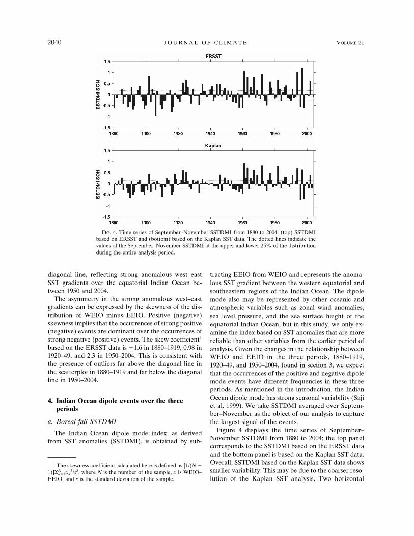
tracting EEIO from WEIO and represents the anoma-lous SST gradient between the western equatorial andsoutheastern regions of the Indian Ocean. The dipolemode also may be represented by other oceanic andatmospheric variables such as zonal wind anomalies,sea level pressure, and the sea surface height of theequatorial Indian Ocean, but in this study, we only ex-amine the index based on SST anomalies that are morereliable than other variables from the earlier period ofanalysis. Given the changes in the relationship betweenWEIO and EEIO in the three periods, 1880–1919,1920–49, and 1950–2004, found in section 3, we expectthat the occurrences of the positive and negative dipolemode events have different frequencies in these threeperiods. As mentioned in the introduction, the IndianOcean dipole mode has strong seasonal variability (Sajiet al. 1999). We take SSTDMI averaged over Septem-ber–November as the object of our analysis to capturethe largest signal of the events.

Figure 4 displays the time series of September–November SSTDMI from 1880 to 2004; the top panelcorresponds to the SSTDMI based on the ERSST dataand the bottom panel is based on the Kaplan SST data.Overall, SSTDMI based on the Kaplan SST data showssmaller variability. This may be due to the coarser reso-lution of the Kaplan SST analysis. Two horizontal

1 The skewness coefficient calculated here is defined as [1/(N �1)]�N

k�1xk3/s3, where N is the number of the sample, x is WEIO–

EEIO, and s is the standard deviation of the sample.

FIG. 4. Time series of September–November SSTDMI from 1880 to 2004: (top) SSTDMIbased on ERSST and (bottom) based on the Kaplan SST data. The dotted lines indicate thevalues of the September–November SSTDMI at the upper and lower 25% of the distributionduring the entire analysis period.

2040 J O U R N A L O F C L I M A T E VOLUME 21

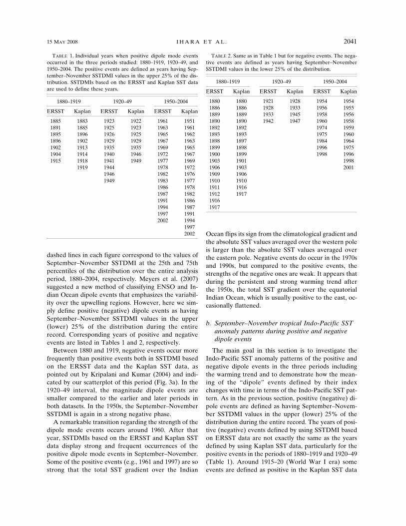
dashed lines in each figure correspond to the values ofSeptember–November SSTDMI at the 25th and 75thpercentiles of the distribution over the entire analysisperiod, 1880–2004, respectively. Meyers et al. (2007)suggested a new method of classifying ENSO and In-dian Ocean dipole events that emphasizes the variabil-ity over the upwelling regions. However, here we sim-ply define positive (negative) dipole events as havingSeptember–November SSTDMI values in the upper(lower) 25% of the distribution during the entirerecord. Corresponding years of positive and negativeevents are listed in Tables 1 and 2, respectively.

Between 1880 and 1919, negative events occur morefrequently than positive events both in SSTDMI basedon the ERSST data and the Kaplan SST data, aspointed out by Kripalani and Kumar (2004) and indi-cated by our scatterplot of this period (Fig. 3a). In the1920–49 interval, the magnitude dipole events aresmaller compared to the earlier and later periods inboth datasets. In the 1950s, the September–NovemberSSTDMI is again in a strong negative phase.

A remarkable transition regarding the strength of thedipole mode events occurs around 1960. After thatyear, SSTDMIs based on the ERSST and Kaplan SSTdata display strong and frequent occurrences of thepositive dipole mode events in September–November.Some of the positive events (e.g., 1961 and 1997) are sostrong that the total SST gradient over the Indian

Ocean flips its sign from the climatological gradient andthe absolute SST values averaged over the western poleis larger than the absolute SST values averaged overthe eastern pole. Negative events do occur in the 1970sand 1990s, but compared to the positive events, thestrengths of the negative ones are weak. It appears thatduring the persistent and strong warming trend afterthe 1950s, the total SST gradient over the equatorialIndian Ocean, which is usually positive to the east, oc-casionally flattened.

b. September–November tropical Indo-Pacific SSTanomaly patterns during positive and negativedipole events

The main goal in this section is to investigate theIndo-Pacific SST anomaly patterns of the positive andnegative dipole events in the three periods includingthe warming trend and to demonstrate how the mean-ing of the “dipole” events defined by their indexchanges with time in terms of the Indo-Pacific SST pat-tern. As in the previous section, positive (negative) di-pole events are defined as having September–Novem-ber SSTDMI values in the upper (lower) 25% of thedistribution during the entire record. The years of posi-tive (negative) events defined by using SSTDMI basedon ERSST data are not exactly the same as the yearsdefined by using Kaplan SST data, particularly for thepositive events in the periods of 1880–1919 and 1920–49(Table 1). Around 1915–20 (World War I era) someevents are defined as positive in the Kaplan SST data

TABLE 1. Individual years when positive dipole mode eventsoccurred in the three periods studied: 1880–1919, 1920–49, and1950–2004. The positive events are defined as years having Sep-tember–November SSTDMI values in the upper 25% of the dis-tribution. SSTDMIs based on the ERSST and Kaplan SST dataare used to define these years.

1880–1919 1920–49 1950–2004

ERSST Kaplan ERSST Kaplan ERSST Kaplan

1885 1883 1923 1922 1961 19511891 1885 1925 1923 1963 19611895 1896 1926 1925 1965 19621896 1902 1929 1929 1967 19631902 1913 1935 1935 1969 19651904 1914 1940 1946 1972 19671915 1918 1941 1949 1977 1969

1919 1944 1978 19721946 1982 19761949 1983 1977

1986 19781987 19821991 19861994 19871997 19912002 1994

19972002

TABLE 2. Same as in Table 1 but for negative events. The nega-tive events are defined as years having September–NovemberSSTDMI values in the lower 25% of the distribution.

1880–1919 1920–49 1950–2004

ERSST Kaplan ERSST Kaplan ERSST Kaplan

1880 1880 1921 1928 1954 19541886 1886 1928 1933 1956 19551889 1889 1933 1945 1958 19561890 1890 1942 1947 1960 19581892 1892 1974 19591893 1893 1975 19601898 1897 1984 19641899 1898 1996 19751900 1899 1998 19961903 1901 19981906 1903 20011909 19061910 19101911 19161912 191719161917

15 MAY 2008 I H A R A E T A L . 2041

but not in the ERSST data. Three positive events dur-ing 1940–45 (World War II era) are captured by theERSST data but not by the Kaplan SST data. However,those differences do not substantially impact the mainresults of this section.

We first confirm the dipole patterns over the IndianOcean using the mean SST anomalies of each period asthe reference state instead of using the entire climatol-ogy from 1880 to 2004. In each period the composites ofthe September–November SST anomalies obtainedfrom the ERSST data over the tropical Indian Oceanduring positive–negative events are compared to thecomposite means including all years of each period, andthe difference between them is tested using a two-sample Student’s t test2 (figures not shown). Significantwarming compared to the mean of the period over thewestern pole and significant cooling compared to themean of the period over the eastern pole are foundduring positive events in all periods. During negativeevents significant cooling over the western pole andsignificant warming over the eastern pole are found in1880–1919 and 1950–2004, but not in 1920–49. Note thatthere are only four negative events during this period.Thus, the dipole variability of the positive and negativeevents is observed in all periods when the different ref-erence states are used in each period. However, whenthe climatology of the entire period is used as the ref-erence state, what do these same positive and negativeevents look like?

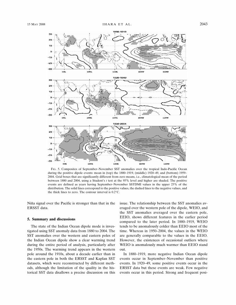
Figure 5 presents the composites of the September–November SST anomalies over the tropical Indo-Pacific Ocean obtained from the ERSST data duringthe positive dipole events; the top panel corresponds tothe mean in 1880–1919, the middle panel is for 1920–49,and the bottom panel for 1950–2004 (see Table 1 for theindividual years). Grid points with values that are sig-nificantly different from the zero means3 compared tothe 1880–2004 climatology at 95% and higher areshaded.

In 1880–1919 and 1920–49, the eastern pole is colderthan normal during the positive dipole events. In 1920–49, the cold anomalies extend over the Maritime Con-tinent and the Southern Hemisphere. In 1880–1919,anomalous warming is observed in the equatorial Pa-

cific. The co-occurrence of the positive Indian Oceandipole events with El Niños (i.e., a warming anomaly inthe eastern equatorial Pacific) is not strong but signif-icant. In 1920–49, there is no significant signal over thetropical Pacific Ocean during positive events except forthe small region in the western South Pacific. The timeseries of SSTDMI and for the Niño-3 region also indi-cate frequent occurrences of weak positive dipoleevents in the absence of Pacific warm events in thisperiod (figure not shown). In 1950–2004, during thepositive dipole mode events, the western pole tends tobe warmer than normal and the eastern pole tends to becolder than normal. It is worth noting that despite thestrong warming trend in this period (shown in section3), the eastern pole still shows significant cooling com-pared to the climatology during the positive dipoleevents. A strong warming signal is displayed over theequatorial eastern Pacific Ocean, indicating that strongEl Niño events tend to co-occur with positive dipoleevents during this period (e.g., 1982, 1997). Significantcooling compared to the climatology over the easternpole is seen during positive events in all three periods,but significant warming compared to the climatologyover the western pole appears only in 1950–2004. Thiscan explain why the strength of the positive dipolemode events is dramatically increased after 1960. Thesame positive events in terms of the dipole mode indexexhibit different SST patterns in three periods when thesame reference is used. We repeated the same analysisusing the Kaplan SST data and obtained similar results,with the El Niño pattern in 1880–1919 composite ap-pearing to be stronger than in the ERSST composites.

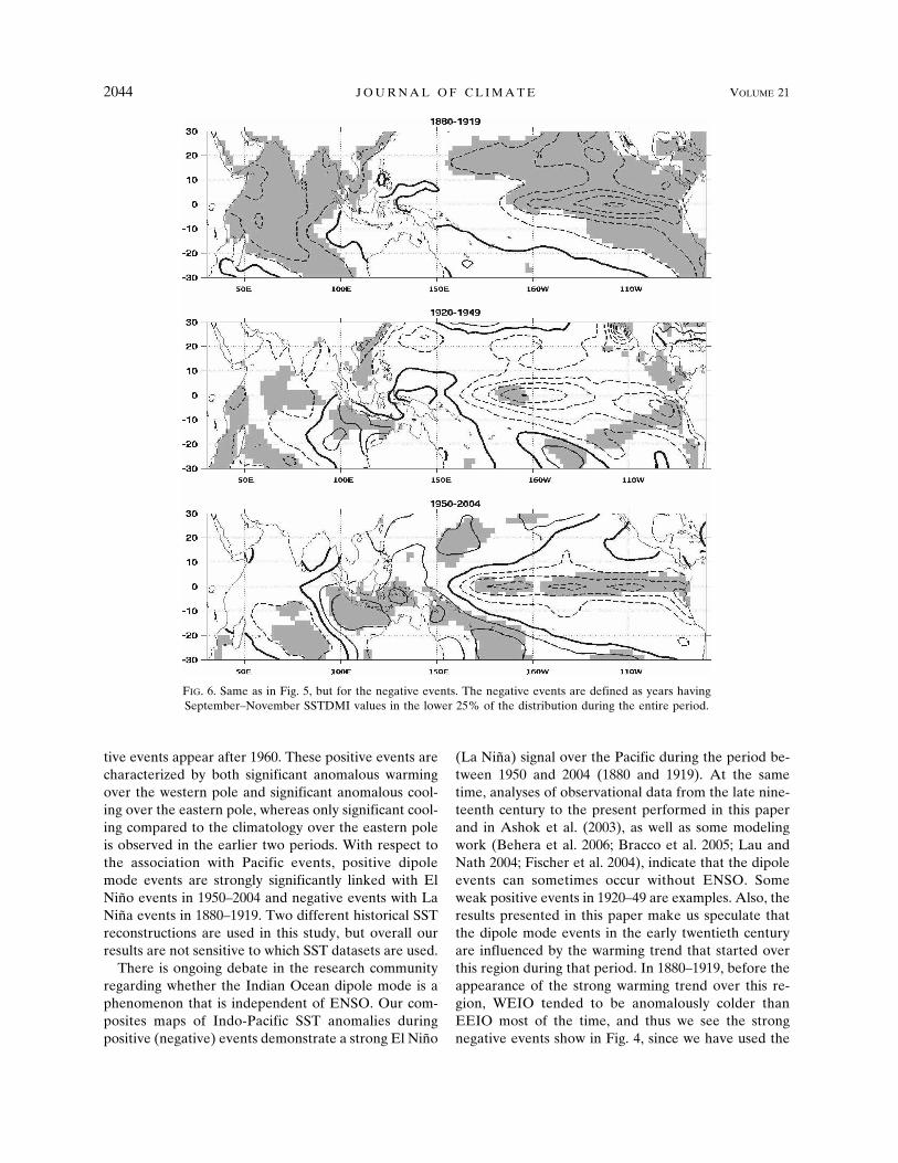
Figure 6 is the same as Fig. 5 but during the negativeevents (see Table 2 for the individual years). In 1880–1919, the Indian Ocean basin is characterized by basin-wide cold anomalies and the absence of significantwarmth over the eastern pole. Over the eastern Pacificthere are significant cold anomalies, implying that thenegative events tends to co-occur with La Niña events.In the 1920–49 interval, there are only four negativeevents; thus, the statistical significance is not robustenough to judge whether a signal is different from thenoise. However, cooling is found over the western poleand warming is found over the eastern pole. La Niñafeatures are seen in the Pacific basin although they arenot significant at the 95% level. In 1950–2004, over theIndian Ocean, the eastern pole is warmer than normaland the southern Indian Ocean is colder than normal,but there is no signal at the western pole. Over theequatorial Pacific Ocean, there is weak but significantcooling. We obtained the same results using the KaplanSST data. However, in 1950–2004, significant coolingover the southern Indian Ocean is not found and the La

2 The test statistics of the two-sample Student’s t test is (�1 ��2)/�(s2

1/ n1 � s22/n2), where �1 and �2 are the means, s1 and s2 the

standard deviations of samples 1 and 2, and n1 and n2 are thenumbers of values in samples 1 and 2, respectively.

3 The test statistics of the Student’s t test is obtained by �/�(s2/n), where � is the mean of the sample, s is the standard deviationof the sample, and n is the number of the sample. It is calculatedusing the mean, standard deviation, and sample number of eachperiod. A two-tailed test is used in this analysis.

2042 J O U R N A L O F C L I M A T E VOLUME 21

Niña signal over the Pacific is stronger than that in theERSST data.

5. Summary and discussions

The state of the Indian Ocean dipole mode is inves-tigated using SST anomaly data from 1880 to 2004. TheSST anomalies over the western and eastern poles ofthe Indian Ocean dipole show a clear warming trendduring the entire period of analysis, particularly afterthe 1950s. The warming trend appears in the westernpole around the 1910s, about a decade earlier than inthe eastern pole in both the ERSST and Kaplan SSTdatasets, which were reconstructed by different meth-ods, although the limitation of the quality in the his-torical SST data disallows a precise discussion on this

issue. The relationship between the SST anomalies av-eraged over the western pole of the dipole, WEIO, andthe SST anomalies averaged over the eastern pole,EEIO, shows different features in the earlier periodcompared to the later period. In 1880–1919, WEIOtends to be anomalously colder than EEIO most of thetime. Whereas in 1950–2004, the values in the WEIOare generally comparable to the values in the EEIO.However, the existences of occasional outliers whereWEIO is anomalously much warmer than EEIO standout.

In 1880–1919, more negative Indian Ocean dipoleevents occur in September–November than positiveevents. In 1920–49, some positive events occur in theERSST data but these events are weak. Few negativeevents occur in this period. Strong and frequent posi-

FIG. 5. Composites of September–November SST anomalies over the tropical Indo-Pacific Oceanduring the positive dipole events: mean in (top) the 1880–1919, (middle) 1920–49, and (bottom) 1959–2004. Grid boxes that are significantly different from zero means, i.e., climatological mean of the periodbetween 1880 and 2004, using a Student’s t test at the 95% level and higher are shaded. The positiveevents are defined as years having September–November SSTDMI values in the upper 25% of thedistribution. The solid lines correspond to the positive values, the dashed lines to the negative values, andthe thick lines to zero. The contour interval is 0.2°C.

15 MAY 2008 I H A R A E T A L . 2043

tive events appear after 1960. These positive events arecharacterized by both significant anomalous warmingover the western pole and significant anomalous cool-ing over the eastern pole, whereas only significant cool-ing compared to the climatology over the eastern poleis observed in the earlier two periods. With respect tothe association with Pacific events, positive dipolemode events are strongly significantly linked with ElNiño events in 1950–2004 and negative events with LaNiña events in 1880–1919. Two different historical SSTreconstructions are used in this study, but overall ourresults are not sensitive to which SST datasets are used.

There is ongoing debate in the research communityregarding whether the Indian Ocean dipole mode is aphenomenon that is independent of ENSO. Our com-posites maps of Indo-Pacific SST anomalies duringpositive (negative) events demonstrate a strong El Niño

(La Niña) signal over the Pacific during the period be-tween 1950 and 2004 (1880 and 1919). At the sametime, analyses of observational data from the late nine-teenth century to the present performed in this paperand in Ashok et al. (2003), as well as some modelingwork (Behera et al. 2006; Bracco et al. 2005; Lau andNath 2004; Fischer et al. 2004), indicate that the dipoleevents can sometimes occur without ENSO. Someweak positive events in 1920–49 are examples. Also, theresults presented in this paper make us speculate thatthe dipole mode events in the early twentieth centuryare influenced by the warming trend that started overthis region during that period. In 1880–1919, before theappearance of the strong warming trend over this re-gion, WEIO tended to be anomalously colder thanEEIO most of the time, and thus we see the strongnegative events show in Fig. 4, since we have used the

FIG. 6. Same as in Fig. 5, but for the negative events. The negative events are defined as years havingSeptember–November SSTDMI values in the lower 25% of the distribution during the entire period.

2044 J O U R N A L O F C L I M A T E VOLUME 21

climatology of the entire period from 1880 to 2004 asthe reference. It can be said that the warming trendappeared earlier in WEIO than in EEIO; thus, the val-ues of WEIO caught up with those of EEIO before thewarming trend started over EEIO. After the 1960s, un-like in the early twentieth century, the values of WEIOare mostly comparable to those of EEIO. However,strong positive events that are characterized by bothsignificantly warmer than normal WEIO and signifi-cantly colder than normal EEIO occasionally appear;something that is not found in the earlier two periods.

It is interesting that the eastern pole sometimes coolsamong the strong warming trend over this region. Incontrast to the surface warming trend of the IndianOcean, Alory et al. (2007) found a subsurface coolingtrend of the main thermocline over the IndonesianThroughflow region, that is, near EEIO, in 1960–99, theinterval using the new Indian Ocean Thermal Archive.Thus, it can be speculated that water carried to thesurface by upwelling during positive dipole events isbecoming colder and results in a colder EEIO duringpositive events in recent decades. We also hypothesizethat shoaling of the thermocline over the EEIO, corre-sponding to a subsurface cooling trend (Alory et al.2007), can make this region more susceptible to thewind–thermocline feedback and leads to frequent oc-currences of positive events in recent decades. Thus,the emergence of intense and frequent positive dipoleevents in recent decades may be speculated to havesome connection to the trend of the climatic conditionsover this region.

Acknowledgments. Authors offer their thanks to Dr.Alexey Kaplan for helpful comments on the datasets.This work was supported by NASA Headquarters un-der Earth System Science Fellowship Grant NGT5.Both YK and MAC were supported under NSF GrantATM0347009.

REFERENCES

Allan, R. J., J. A. Lindesay, and C. J. C. Reason, 1995: Multide-cadal variability in the climate system over the Indian Oceanregion during the austral summer. J. Climate, 8, 1853–1873.

——, and Coauthors, 2001: Is there an Indian Ocean dipole, andis it independent of the El Niño–Southern Oscillation?CLIVAR Exchanges, Vol. 6, No. 3, International CLIVARProject Office, Southampton, United Kingdom, 18–22.

Alory, G., S. Wijffels, and G. Meyers, 2007: Observed tempera-ture trends in the Indian Ocean over 1960–1999 and associ-ated mechanisms. Geophys. Res. Lett., 34, L02606,doi:10.1029/2006GL028044.

Annamalai, H., J. Potemra, R. Murtugudde, and J. P. McCreary,2005: Effect of preconditioning on the extreme climate eventsin the tropical Indian Ocean. J. Climate, 18, 3450–3469.

Ashok, K., Z. Guan, and T. Yamagata, 2001: Impact on the Indian

Ocean dipole on the relationship between the Indian mon-soon rainfall and ENSO. Geophys. Res. Lett., 28, 4499–4502.

——, ——, and ——, 2003: A look at the relationship between theENSO and the Indian Ocean dipole. J. Meteor. Soc. Japan,81, 41–56.

——, W. Chan, T. Motoi, and T. Yamagata, 2004a: Decadal vari-ability of the Indian Ocean dipole. Geophys. Res. Lett., 31,L24207, doi:10.1029/2004GL021345.

——, Z. Guan, N. H. Saji, and T. Yamagata, 2004b: Individual andcombined influences of the ENSO and the Indian Ocean di-pole on the Indian summer monsoon. J. Climate, 17, 3141–3154.

Behera, S. K., J. J. Luo, S. Masson, P. Delecluse, S. Gualdi, A.Navarra, and T. Yamagata, 2005: Paramount impact of theIndian Ocean dipole on the East African short rains: ACGCM study. J. Climate, 18, 4514–4530.

——, ——, ——, S. A. Rao, H. Sakuma, and T. Yamagata, 2006:A CGCM study on the interaction between IOD and ENSO.J. Climate, 19, 1688–1705.

Bracco, A., F. Kucharski, F. Molteni, W. Hazeleger, and C. Sever-ijns, 2005: Internal and forced modes of variability in theIndian Ocean. Geophys. Res. Lett., 32, L12707, doi:10.1029/2005GL023154.

Chang, P., and Coauthors, 2006: Climate fluctuations of tropicalcoupled system—The role of ocean dynamics. J. Climate, 19,5122–5174.

Clark, C. O., P. J. Webster, and J. E. Cole, 2003: Interdecadalvariability of the relationship between the Indian Oceanzonal mode and East African coastal rainfall anomalies. J.Climate, 16, 548–554.

Fischer, A. S., P. Terray, E. Guilyardi, S. Gualdi, and P. Delec-luse, 2004: Two independent triggers for the Indian Oceandipole/zonal mode in a coupled GCM. J. Climate, 18, 3428–3449.

Guan, Z., and T. Yamagata, 2003: The unusual summer of 1994 inEast Asia: IOD teleconnections. Geophys. Res. Lett., 30,1544, doi:10.1029/2002GL016831.

Hurrell, J. W., and K. E. Trenberth, 1999: Global sea surface tem-perature analyses: Multiple problems and their implicationsfor climate analysis, modeling, and reanalysis. Bull. Amer.Meteor. Soc., 80, 2661–2678.

Ihara, C., Y. Kushnir, and M. A. Cane, 2008: July droughts overthe homogeneous Indian monsoon region and Indian Oceandipole during El Niño events. Int. J. Climatol., in press.

Jones, P. D., D. E. Parker, T. J. Osborn, and K. R. Briffa, 2006:Global and hemispheric temperature anomalies—Land andmarine instrumental records. Trends: A Compendium of Dataon Global Change, Carbon Dioxide Information AnalysisCenter, Oak Ridge National Laboratory, U.S. Department ofEnergy, Oak Ridge, TN.

Kaplan, A., M. Cane, Y. Kushnir, A. Clement, M. Blumenthal,and B. Rajagopalan, 1998: Analyses of global sea surfacetemperature 1856–1991. J. Geophys. Res., 103, 18 567–18 589.

——, M. A. Cane, and Y. Kushnir, 2003: Reduced space approachto the optimal analysis interpolation of historical marine ob-servations: Accomplishments, difficulties, and prospects. Ad-vances in the Applications of Marine Climatology: The Dy-namic Part of the WMO Guide to the Applications of MarineClimatology, WMO/TD-1081, World Meteorological Organi-zation, Geneva, Switzerland, 199–216.

Kripalani, R. H., and P. Kumar, 2004: Northeast monsoon rainfallvariability over south peninsular India vis-à-vis the IndianOcean dipole mode. Int. J. Climatol., 24, 1267–1282.

15 MAY 2008 I H A R A E T A L . 2045

——, J. H. Oh, J. H. Kang, S. S. Sabade, and A. Kulkarni, 2005:Extreme monsoons over East Asia: Possible role of IndianOcean zonal mode. Theor. Appl. Climatol., 82, 81–94.

Kulkarni, A., S. S. Sabade, and R. H. Kripalani, 2007: Associationbetween extreme monsoons and the dipole mode over theIndian subcontinent. Meteor. Atmos. Phys., 95, 255–268.

Lau, N.-C., and M. J. Nath, 2004: Coupled GCM simulation ofatmosphere–ocean variability associated with zonally asym-metric SST changes in the tropical Indian Ocean. J. Climate,17, 245–265.

Li, T., B. Wang, C.-P. Chang, and Y. S. Zhang, 2003: A theory forthe Indian Ocean dipole–zonal mode. J. Atmos. Sci., 60,2119–2135.

Meyers, G., P. McIntosh, L. Pigot, and M. Pook, 2007: The yearsof El Niño, La Niña, and interactions with the tropical IndianOcean. J. Climate, 20, 2872–2880.

Reverdin, G., D. L. Cadet, and D. Gutzler, 1986: Interannual dis-placements of convection and surface circulation over theequatorial Indian Ocean. Quart. J. Roy. Meteor. Soc., 112,43–67.

Saha, K., 1970: Zonal anomaly of sea surface temperature in equa-torial Indian Ocean and its possible effect upon monsooncirculation. Tellus, 4, 403–409.

Saji, N. H., and T. Yamagata, 2003: Possible impacts of Indian

Ocean dipole mode events on global climate. Climate Res.,25, 151–169.

——, B. N. Goswami, P. N. Vinayachandran, and T. Yamagata,1999: A dipole mode in the tropical Indian Ocean. Nature,401, 360–363.

Slutz, R. J., S. J. Lubker, J. D. Hiscox, S. D. Woodruff, R. L.Jenne, D. H. Joseph, P. M. Steuer, and J. D. Elms, 1985:Comprehensive Ocean–Atmosphere Data Set: Release 1.NOAA/Environmental Research Laboratories/Climate Re-search Program, Boulder, CO, 268 pp. [NTIS PB86-105723.]

Smith, T. M., and R. W. Reynolds, 2003: Extended reconstructionof global sea surface temperatures based on COADS data(1854–1997). J. Climate, 16, 1495–1510.

——, and ——, 2004: Improved extended reconstruction of SST(1854–1997). J. Climate, 17, 2466–2477.

Terray, P., and S. Dominiak, 2005: Indian Ocean sea surface tem-perature and El Niño–Southern Oscillation: A new perspec-tive. J. Climate, 18, 1351–1368.

Tozuka, T., J. J. Luo, S. Masson, and T. Yamagata, 2007: Decadalmodulations of the Indian Ocean dipole in the SINTEX-F1coupled GCM. J. Climate, 20, 2881–2894.

Webster, P. J., A. M. Moore, J. P. Loschnigg, and R. R. Leben,1999: Coupled ocean–atmosphere dynamics in the IndianOcean during 1997–98. Nature, 401, 356–360.

2046 J O U R N A L O F C L I M A T E VOLUME 21