warehouse optimisation at abb - diva portal

Margrét Björgvinsdóttir

Vt 2015

Examensarbete, 30 hp

Industriell ekonomi, inriktning logistik och optimering 300 hp

Warehouse Optimisation at ABB

Finding strategic locations for incoming warehouse items using operational research methods

Margrét Björgvinsdóttir

Abstract

Warehouse Management Systems, WMS, contributes to new opportunities concerning strategies in the placement of items in a warehouse. The department Components in ABB Ludvika implemented the system in the spring of 2015. The

purpose of this thesis and project is to find new strategies for placing items in the warehouse and give suggestions that increase the efficiency and reduce the time

spent on order picking. In the project a program was written in C-code where time is presented as cost. The program gives suggested placements for all items in the warehouse, size of shelves and batches taken into account, and presents the cost reduction. A heuristic method within the field of operational research is used and

the result shows improvements by 20-30 percent compared to the cost of the present placements. Routines for usage concerning the delivered program are suggested. Storage policies are also discussed and further improvements are

suggested.

Sammanfattning

Ett Warehouse Management Systems, WMS, bidrar med nya möjligheter vad gäller strategiska placeringar av artiklar i ett lager. Avdelningen Components på ABB i Ludvika implementerade ett sådant system under våren 2015. Syftet med detta

examensarbete är att hitta nya strategier för placeringar och ge förslag för att öka effektiviteten och reducera plocktiden. Under projektet skrevs ett program i

programmeringsspråket C där tiden representeras som en kostnad. Programmet ger förslag på placeringar för artiklarna i lagret, där hyllornas och

artikelförvaringarnas storlekar tagits med i beräkningen, och presenterar kostnadsreduceringen. En heuristisk metod inom operationsanalys har använts

och visar förbättringar på 20-30 procent jämfört med den ursprungliga kostnaden. I arbetet finns föreslagna rutiner för användningen av programmet. Lagerpolicies är även diskuterade och förslag på ytterligare förbättringar ges.

Contents

1. Introduction ____________________________________________________________________________________________________4

1.1 ABB Transformer components; On-load tap changers _____________________________________________________4

1.1.1 Material flow in Components Warehouse ______________________________________________________________4

1.1.2 Order picking _____________________________________________________________________________________________5

1.2 Project _________________________________________________________________________________________________________5

1.2.1 Aim of the project ________________________________________________________________________________________5

1.2.2 Limitations and constraints _____________________________________________________________________________5

1.2.2.1 Limitations of data _____________________________________________________________________________________6

1.2.2.2 Limitations in the model ______________________________________________________________________________6

1.2.2.3 Drawers and kitting ____________________________________________________________________________________6

1.3 Data ____________________________________________________________________________________________________________7

1.3.1 Shelves ____________________________________________________________________________________________________7

1.3.2 Incoming batches to T30 ________________________________________________________________________________7

1.3.3 Items in the warehouse __________________________________________________________________________________8

2. Theory – Literature review ____________________________________________________________________________________8

2.1 Warehouse theory ____________________________________________________________________________________________8

2.1.1 Lean warehouses _________________________________________________________________________________________8

2.1.2 Storage policies __________________________________________________________________________________________9

2.2 Optimisation theory __________________________________________________________________________________________9

2.2.1 Multiple-Level Warehouse Layout Problem -MLWLP _________________________________________________9

2.2.2 Model Assumptions ____________________________________________________________________________________ 10

2.2.3 Mathematical model ___________________________________________________________________________________ 10

2.2.4 Problem description ___________________________________________________________________________________ 11

2.2.5 0-1 NP-hard integer programs ________________________________________________________________________ 11

2.2.6 Simulated Annealing ___________________________________________________________________________________ 11

2.2.6.1 Simulated Annealing - model________________________________________________________________________ 11

2.2.4.2 Simulated Annealing - parameters__________________________________________________________________ 12

3. Method ________________________________________________________________________________________________________ 13

3.1 Modified MLWLP ____________________________________________________________________________________________ 13

3.2 Simulated Annealing ________________________________________________________________________________________ 14

3.2.1 Initial solution __________________________________________________________________________________________ 14

3.2.2 The Simulated Annealing optimisation program ____________________________________________________ 15

3.2.3 Program initialisation _________________________________________________________________________________ 15

3.3 Optimisation _________________________________________________________________________________________________ 15

3.3.1 Parameters _____________________________________________________________________________________________ 16

3.4 Simulations and data _______________________________________________________________________________________ 16

3.4.1 Data _____________________________________________________________________________________________________ 16

3.4.2 Adding an extended dataset ___________________________________________________________________________ 17

4. Results _________________________________________________________________________________________________________ 17

4.1 The extended dataset ____________________________________________________________________________________ 19

4.2 Comparing results to lower bounds ____________________________________________________________________ 19

4.3 Adding data for items without order pick frequency __________________________________________________ 19

4.4 Influential items in the reduced dataset ________________________________________________________________ 21

5. Discussion _____________________________________________________________________________________________________ 22

5.1 Results _______________________________________________________________________________________________________ 22

5.1.1 Results – Comparing the reduced with the extended dataset ______________________________________ 22

5.1.2 Strategies and further improvements for updating the items locations ___________________________ 22

5.1.3 Dedicated storage policies _____________________________________________________________________________ 23

5.1.4 Including drawers; further improvements ___________________________________________________________ 24

5.2 Method _______________________________________________________________________________________________________ 24

5.3 Validation of data ___________________________________________________________________________________________ 24

6. Conclusion ____________________________________________________________________________________________________ 24

Bibliography _____________________________________________________________________________________________________ 26

(27)

1. Introduction

In the spring 2015 a WMS, Warehouse Management System, was installed in Components central

warehouse. This enabled new order picking systems. Before the installation, the warehouse items were

mostly sectioned by production line and/or groups such as motors, wires, cabinets etc. The previous

system is used to make it easier for personnel to locate items without login on to the ERP-LN or know

every item location by heart, they only have to know the system. This system is not flexible and items get

positions that may not be optimal from a transportation aspect.

1.1 ABB Transformer components; On-load tap changers

ABB is a global leader in automation and power technologies. The company has a history of technological

innovations such as the ultra-efficient high-voltage direct current power transmission that is produced in

Ludvika, Sweden. ABB employs 145,000 people around the world and operates in approximately 100

countries. (About ABB in brief, 2015)

Components is a division within ABB Power Products and is located in Ludvika, Sweden. Components has

produced components to power transformers since the beginning of the 19th century. The department is

ABB’s largest production of on-load tap chargers, OLTC, and IEC Current Transformers. (ABB i Sverige-

Components, 2015)

Figur 1. The OLTC-lines and warehouse of Components

The production lines are located as shown in Figure 1. (UB, UC, UZ and DON). The red arrow in marks the

in- and output port, I/O-port, which the items are transported thru to get to the production lines.

1.1.1 Material flow in Components Warehouse

The storage units that are delivered by subcontractors first arrive at the incoming section of the

Component warehouse, marked X in Figure 1..The department has a large warehouse, the central

warehouse called T30, and smaller warehouse sections in other parts of the department. After being

scanned in the units are moved by trucks to their location in the warehouse. The scanners are connected to

the computer system, called ERP LN, for stock levels. T30 has 1841 shelves in six aisles, A-F. The aisles

have between 28 and 38 columns and the columns have between 6 and 12 levels from floor to top. UB-line

has its own warehouse aisles in the UB-area, see Figure 1. When there is a demand in the production for an

item, the truck-driver finds its location, then collects and delivers it to the production-lines. Some items

are family grouped1 and have specific aisles for a specific production-line.

1.1.2 Order picking

The items are collected differently depending on size and which line and/or part of the line they are to be

delivered to. The items of concern in this thesis project are collected by truck, one item-sort at a time but

in various amounts. The items are delivered on demand to the production lines.

The WMS system includes barcode scanners that are used for order picking. The items are scanned when

delivered and the scanners propose a location for the item in the warehouse. The scanner is used to find

items in the warehouse when needed. When an item is moved from the warehouse to the production lines

the item is ‘checked out’ from the warehouse and into the production. This gives a real-time inventory, a

snapshot of reality, in the material flow.

The implementation of the WMS enabled new possibilities in handling the order picking. The personnel

no longer need to know where items are located, and not be restricted to certain areas, the items locations

can therefore be optimised from a time aspect instead.

1.2 Project

1.2.1 Aim of the project

The department Components at ABB Ludvika use a Warehouse Management System, WMS, in the

production- and central warehouse. The WMS gives suggested locations for incoming warehouse items in

the central warehouse or other locations such as UB-Line storage. The locations, as they are set today, are

fixed to positions which are given when an item is delivered for the first time. The purpose of this project

and thesis is to optimise warehouse layout by finding strategic locations for incoming items to reduce the

time for order picking by operational research.

1.2.2 Limitations and constraints

There are some limitations due to lack of data and simplifications have been made to limit the effects of

these lacking in the project.

1 Definition in theory chapter 2.1.2 Storage policies

1.2.2.1 Limitations of data

Due to the lack of data regarding sizes of batches and locations for the batches simplifications are made.

The batches can be delivered in sizes from one to six collars high. A collar is a standardised industry size

according to ABB personnel (Strandberg, E. 2015, pers.comm., 5 may). The batches have one or multiple

locations after the installation of the WMS, i.e. they are located on multiple locations. To handle this, the

program stores the largest location size of multiple locations as the batch size. This could be misleading

because if multiple items are stored in the same shelf it means that the batch is smaller than the location

size it is placed in. The WMS-system is limited to store one location per item and that is therefore a

constraint in the model. The alternative, to take a mean value of the multiple sizes, could lead to lack in

storage capacity for the fixed location and is therefore rejected. Assigning a batch to a location that it does

not fit in is more problematic than assigning it to a larger one.

The data from ERP-LN is accurate and up to date. The data is collected from the past year. An alternative

could be to use prognoses or assumptions about the future but that is considered to be outside the scope of

this thesis project. The model is made as adaptable and flexible as possible so that it can be used to update

the locations when necessary.

Not all items have data on order picking frequency. This limits the items in the model. There are about

500 of the items that are excluded in the original dataset. To get a better appreciation of the complete

warehouse, including the items that lack data, simulations are done with an extended data for order pick

frequency.2

1.2.2.2 Limitations in the model

A simplification that is made in the objective function is regarding the transportation cost. The cost is

simplified and approximated. The cost for picking an item is the approximate time for moving from the

cell to the I/O-port and an additional cost of 4 seconds if the location is above a specific limit. The limit is

because above a certain height the truck driver has to unfold safety armature. Because the shelves have

different dimensions the limit is not the same for all columns of the warehouse but an approximated

mean.

The model can only dedicate each item one location. The most frequently used items use more than one

location in reality, this is further discussed in 5.1.3 Dedicated storage policies.

1.2.2.3 Drawers and kitting

Some locations are drawers and are therefore extensible. These drawers contain smaller items and often

contain more than one item sort, i.e. article number. The kitting contains items that are small enough to be

collect by hand and are often order specific. The kitting is located in the extensible drawers because of the

item sizes and that the extensible drawers are in picking height, they are reachable without any tools. The

2 More in 3.4.2 Simulation comparison

extensible drawers are mostly stored in family-grouping, both the items within the drawers and the

neighbours. That is, items that are similar or belong to the same kitting are stored in the same area. This

correlation between items makes the optimisation including them more complex. This problem is

considered a sub-problem and is therefore separated from the optimisation. Due to the time constraint of

this thesis project this problem is excluded.

1.3 Data

ERP LN is the computerised system used which contains data about items, orders, locations etc. Not all

data is computerised and is therefore collected manually if needed. Validation of computerised data is

discussed with employees from the division strategic-purchasing and programmers knowledgeable within

the system.

1.3.1 Shelves

The sizes of the storage shelves were collected by hand due to lack of computerised data. The shelves were

divided into six sizes depending on notches in the rack. The batches that the items are delivered in, mostly

used to store the items in the storage, are between one and six collars hence the division of six sizes.3

Selected areas have drawers for smaller items that are handpicked or kitted. The drawers can contain

multiple items and smaller batches. These specific drawers are of size 1 or 2.

1.3.2 Incoming batches to T30

A batch is a quantity of items taken together, in this case one or a number of items of the same sort in a

wooden box .The batches are from subcontractors and do not have sizes recorded in the system. The sizes

of the batches are a necessary input in the model. To get an approximation of the batch sizes, the batches

current location is matched to the collected location sizes. To make the matches between the two datasets

an extra function was written in the C-program. This function can be called if necessary or if all batch sizes

are available the function is ignored. The data for the program is collected after the implementation of the

WMS, from ERP LN, to get the most accurate description.

3 Explained in 1.2.2.1 Limitations of data

1.3.3 Items in the warehouse

The data for the items is from ERP LN, collected by hand or from personnel:

• Items with fixed positions outside the central warehouse are excluded

• Items with zero usage within the last 12 months are excluded

• Items that are to be excluded from ordering or replaced (flagged in the ERP-LN) are excluded.

• Order picking frequencies are taken from the program QlickView. The frequency shows how many

times per year the item is collected.

• The kitting and drawers data is collected from kitting-personnel.

• Information about the drawers is collected into the dataset by hand. Data on which items that are

stored in the drawers is taken from ERP-LN and data on those items is excluded from the

programs dataset.

2. Theory – Literature review

2.1 Warehouse theory

2.1.1 Lean warehouses

According to the Lean philosophy a reduction of non-value adding activities and an optimisation of value

adding activities are requirements in leaning the warehouse operations in terms of cost and time. In

reducing the non-value adding activities, efficiency of warehouse operations is necessary. These

efficiencies depend on the material handling techniques, media of transportation, and layout

arrangements (Dharmapriya, U.S.S. & Kulatunga A.K., 2011, s. 513). Major warehouse operations can be

activities such as kitting away4, receiving, order picking, storing, sorting, and shipping. According to

Koster et al. (2007), order picking is the most labor-intensive activity amongst these operations. Order

picking can be described as the retrieval of an article from its location in the storage and its delivery to

production, or further process such as transportation (Rouwenhorst, B. et al., 1999, s. 517).

4 See chapter 1.2.2.3

2.1.2 Storage policies

Koster et al. (2007) suggests that there are five frequently used types of storage assignment policies.

Rouwenhorst, et al.,(1999) describes them in short as follows:

• In the random storage policy, the choice of storage locations is dedicated to the operator to

determine.

• In a dedicated storage policy the items are suggested, contradictory to random storage policy, to

have their own particular location.

• A class based storage policy (ABC zoning) divides the products into classes or groups and allocates

them to zones based on these classes. A commonly used parameter for this class division is turnover

rate.

• Family grouping and correlated storage takes into account items that are often required

simultaneously and therefore preferably stored nearby each other.

(Rouwenhorst, B. et al., 1999, s. 517) Family grouping can also be combined with the other storage policies

(De Koster, R., et al., 2007, s. 14).

2.2 Optimisation theory

The operation in a warehouse concerning order picking has a cost in terms of time consumed. The items in

a warehouse have transportation costs both vertically and horisontally. The horisontal cost represents the

transportation from the location of the item along the aisle to the I/O-port and to the production line. If

there is not more than one I/O-port the transportation between the port and the production line is

insignificant. The following chapter follows a general description of the Multiple-Level Warehouse Layout

Problem (MLWPL). The model presented in this chapter is a general version to describe the problem. In

chapter 3. a modified version of the MLWLP is developed for solving the problem at ABB in Ludvika.

2.2.1 Multiple-Level Warehouse Layout Problem -MLWLP

The goal of the multiple-level warehouse layout problem, MLWLP, is to minimise the total transportation

cost both horizontally and vertically. Each item is assigned to one and only one cell or location. One item

type can only be stored in one cell, but one cell can store more than one type of items. The problem is

viewed as NP-hard.5

5 see 2.2.3

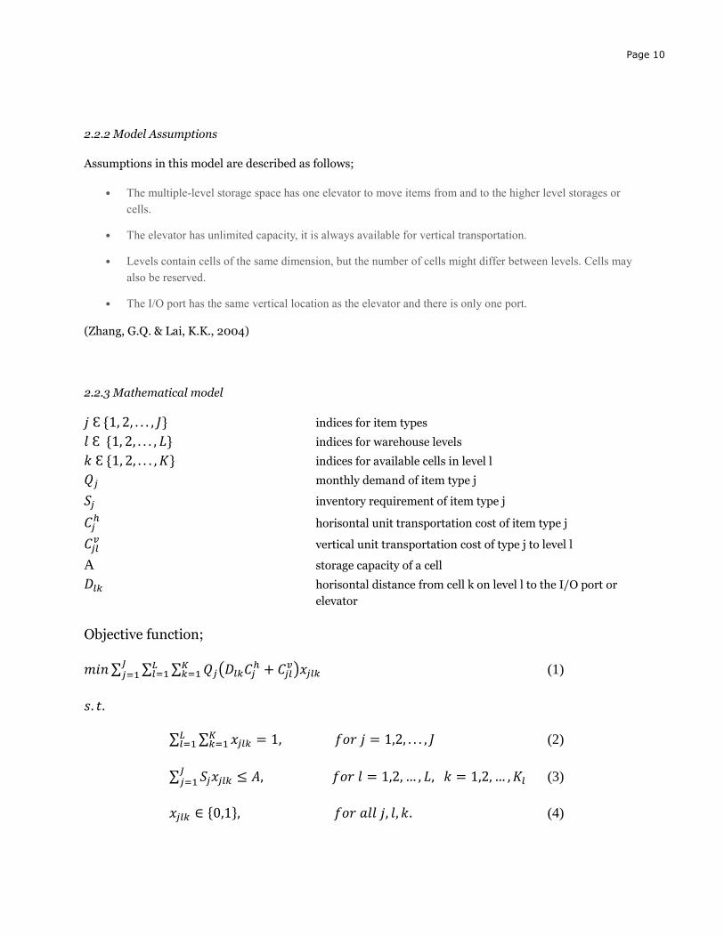
2.2.2 Model Assumptions

Assumptions in this model are described as follows;

• The multiple-level storage space has one elevator to move items from and to the higher level storages or

cells.

• The elevator has unlimited capacity, it is always available for vertical transportation.

• Levels contain cells of the same dimension, but the number of cells might differ between levels. Cells may

also be reserved.

• The I/O port has the same vertical location as the elevator and there is only one port.

(Zhang, G.Q. & Lai, K.K., 2004)

2.2.3 Mathematical model

𝑗 Ԑ {1, 2, . . . , 𝐽} indices for item types

𝑙 Ԑ {1, 2, . . . , 𝐿} indices for warehouse levels

𝑘 Ԑ {1, 2, . . . , 𝐾} indices for available cells in level l

𝑄𝑗 monthly demand of item type j

𝑆𝑗 inventory requirement of item type j

𝐶𝑗ℎ horisontal unit transportation cost of item type j

𝐶𝑗𝑙𝑣 vertical unit transportation cost of type j to level l

A storage capacity of a cell

𝐷𝑙𝑘 horisontal distance from cell k on level l to the I/O port or

elevator

Objective function;

𝑚𝑖𝑛 ∑ ∑ ∑ 𝑄𝑗(𝐷𝑙𝑘𝐶𝑗ℎ + 𝐶𝑗𝑙

𝑣)𝑥𝑗𝑙𝑘𝐾𝑘=1

𝐿𝑙=1

𝐽𝑗=1 (1)

𝑠. 𝑡.

∑ ∑ 𝑥𝑗𝑙𝑘 = 1, 𝑓𝑜𝑟 𝑗 = 1,2, . . . , 𝐽𝐾𝑘=1

𝐿𝑙=1 (2)

∑ 𝑆𝑗𝑥𝑗𝑙𝑘 ≤ 𝐴, 𝑓𝑜𝑟 𝑙 = 1,2, … , 𝐿, 𝑘 = 1,2, … , 𝐾𝑙𝐽𝑗=1 (3)

𝑥𝑗𝑙𝑘 ∈ {0,1}, 𝑓𝑜𝑟 𝑎𝑙𝑙 𝑗, 𝑙, 𝑘. (4)

2.2.4 Problem description

The warehouse is constructed with cells, k, on different levels, l. The items, j, are to be assigned one cell

each. The goal is to minimise the transportation costs which are expressed in the objective function. The

cost is a vertical transportation cost of moving item from the floor to level, l, and the horizontal cost for

moving an item one meter, which is multiplied with the horizontal distance from cell k to the I/O port. The

decision variable is binary and has value 1 if item is designated for a cell, otherwise 0. The cells have a

maximum storage capacity, A, which the inventory requirements for an assigned item may not exceed. The

cells can store more than one item as long as the storage capacity is not violated.

2.2.5 0-1 NP-hard integer programs

A version of a 0-1 integer program is the Knapsack-problem. It is one of the simplest formulations of a

zero-one program. (Lundgren, J., Rönnqvist, M. & Värbrand, P., 2011, s. 330) The 0-1 knapsack problem is

NP-hard (Pochet, Y. & Wolsey, L., A., 2000, s. 274). The MLWLP can be reduced to a 0-1 Knapsack-

problem and is therefore also NP-hard.

According to Abramson et al(1996) there are two ways of solving 0-1 integer problems. Either it is solved

exactly or an appropriate heuristic algorithm is used, usually a problem specific heuristic. Many practical

problems are NP-hard and there are multiple different heuristic methods to solve those such as Tabu

Search, Greedy Search, Local search and Simulated Annealing. Both Tabu Search and Simulated

Annealing are improved local exchange heuristics and include ways to escape from a local optimum

(Wolsey, 1998, s. 204).

2.2.6 Simulated Annealing

The Simulated Annealing, S.A., heuristic picks a random neighbor and replaces it with a new one if the

new solution is a better one, according to the objective function, or if the probability from the temperature

allows it to. The probability depends on the present temperature and the cost of switching the neighbors,

i.e. the difference in the results of the objective function. The temperature decreases with time and

henceforth the chance of making a move to a worse solution. Initially the solution might get worse, more

costly, but with sufficiently large number of iterations the solution will always end up converging towards

a local minimum. (Wolsey, 1998, s. 208)

2.2.6.1 Simulated Annealing - model

𝑇𝐼 Initial temperature, diverges by time

0 < 𝑟 < 1 The reduction factor

𝑆 Initial solution L Loop variable/Epoch length

𝑊ℎ𝑖𝑙𝑒 𝑛𝑜𝑡 𝑓𝑟𝑜𝑧𝑒𝑛 𝑑𝑜: a. 𝑃𝑒𝑟𝑓𝑜𝑟𝑚 𝑓𝑜𝑙𝑙𝑜𝑤𝑖𝑛𝑔 𝐿 𝑡𝑖𝑚𝑒𝑠

i. 𝑅𝑎𝑛𝑑𝑜𝑚 𝑛𝑒𝑖𝑔ℎ𝑏𝑜𝑟 𝑆’ 𝑜𝑓 𝑆

ii. 𝛥 = 𝑓(𝑆’) − 𝑓(𝑆)

iii. 𝑖𝑓 𝛥 ≤ 0, 𝑠𝑒𝑡 𝑆 = 𝑆’

iv. 𝑖𝑓 𝛥 ≥ 0, 𝑠𝑒𝑡 𝑆 = 𝑆’ 𝑤𝑖𝑡ℎ 𝑝𝑟𝑜𝑏𝑎𝑏𝑖𝑙𝑖𝑡𝑦 𝑒−𝛥

𝑇

b. 𝑆𝑒𝑡 𝑇 ← 𝑟𝑇, 𝑟𝑒𝑑𝑢𝑐𝑖𝑛𝑔 𝑡ℎ𝑒 𝑡𝑒𝑚𝑝𝑒𝑟𝑎𝑡𝑢𝑟𝑒

𝑅𝑒𝑡𝑢𝑟𝑛 𝑡ℎ𝑒 𝑏𝑒𝑠𝑡 𝑠𝑜𝑙𝑢𝑡𝑖𝑜𝑛.

The definitions temperature, cooling ratio, loop length and “frozen” have to be specified numerically.

(Wolsey, 1998, s. 208)

2.2.4.2 Simulated Annealing - parameters

The initial temperature determines the initial probability of accepting solutions or steps. Wolsey

suggests choosing that the probability of accepting a transition is:

𝑒−𝛥

𝑇⁄ (5)

This probability is called the initial acceptance probability. A too high initial temperature is known to

cause bad performance or high use of CPU-time but initially the solutions should have a probability to

accept transitions close to 1. (Park, M.-W. & Kimt, Y.-D., 1998)

Different cooling functions are proposed throughout the literature. The cooling can be set with a

proportional cooling function which is common. The cooling function is the reduction of T by the

reduction factor, or reduction ratio, r. One option of finding a suitable r, proposed by Potts and Van

Wassenhove is:

𝑟 = (𝑇𝑀

𝑇𝐼)

1

𝑀−1 (6)

where M is the total number of epochs and 𝑇𝑀 is the temperature at the final epoch. If a slower cooling

than the proportional cooling function is preferred, Lundy and Mees suggest temperature be given by:

𝑇𝑘 =𝑇𝑘−1

1+𝛽𝑇𝑘−1, 𝛽 > 𝑂. (7)

where 𝛽 =𝑇𝐼 − 𝑇𝑀

(𝑀− 1)𝑇𝐼𝑇𝑀 (8)

The loop or the epoch length can be selected in proportion to the size of the problem instance, such as

in the case of MLWLP, where L can be set equal to the number of cells or items in the warehouse. Other

options are setting the L to the total number of trials of the neighborhood solutions that are generated.

The stopping condition can be a predetermined maximum count or a value depending on the CPU-time

(Park, M.-W. & Kimt, Y.-D., 1998, s. 209).

The stopping condition and the definition of frozen varies in the literature. The total number of

epochs can be predetermined and simulations terminated when it is reached. The total number of trials,

limitations of CPU time, or the temperature itself can also be predetermined and used as a stopping

condition. (Park, M.-W. & Kimt, Y.-D., 1998, s. 209) Another method concerning the temperature is

Johnson’s stopping rule which considers the percentage of accepted moves in an epoch (Johnson et al.

161).

According to Park, M.-W and Kimt, Y.-D. it is difficult to select all the variables so that the S.A. gives the

best performance. This is because all the parameters have to be selected and determined at the same time.

Some values for the parameters need to be decided simultaneously because of the correlation between

them, which complicates the choices (Park, M.-W. & Kimt, Y.-D., 1998, s. 209).

3. Method

Because the problem is NP-hard6 the heuristic method of Simulated Annealing is used. The MLWLP is

modified to represent the given parameters and the problem definition. The drawers are considered a sub-

problem, see chapter 1.2.3., and are separated initially from the dataset.

3.1 Modified MLWLP

There is only one I/O-port in T30, see Figure 1., and it has the same vertical location as the elevator which

is an assumption in the MLWLP. In the modification of the MLWLP the cells are not allowed to store more

than one item. This is a request from ABB because storing more than one item in the shelves costs

additional time, retrieving items lying under other items. Because of the different sizes of items and

locations the levels in the model do not contain the same dimensions as in the original MLWLP.

𝑖 Ԑ {1,2,...,𝐼} Indices for item types

𝑗 Ԑ {1, 2,..., 𝐽} Indices for cell size category

𝑘 Ԑ {1, 2,..., 𝐾} Indices for cell in size category

𝑄𝑖 Order pick frequency of item type i

𝑆𝑖 Size of batch for item i

𝐶𝑗𝑘 Total transportation cost from cell 𝑗𝑘 to I/O-port

𝐴𝑗𝑘 Size of cell 𝑗𝑘

𝑥𝑖𝑗𝑘 Item i at cell jk

6 See chapter 2.2.3

𝑚𝑖𝑛 ∑ ∑ ∑ 𝑄𝑖𝐶𝑗𝑘𝑥𝑖𝑗𝑘𝐾𝑘=1

𝐽𝑗=1

𝐽𝑖=1 (9)

s.t.

∑ 𝑆𝑖𝑥𝑖𝑗𝑘 ≤ 𝐴𝑗𝑘𝐼𝑖=1 𝑓𝑜𝑟 𝑎𝑙𝑙 𝑗 𝑎𝑛𝑑 𝑘 (10)

𝐴𝑗𝑘 = {1,2, . . ,6}, 𝑆𝑖 = {1,2, . . ,6}

∑ 𝑥𝑖𝑗𝑘 ≤ 1 𝐼𝑖=1 𝑓𝑜𝑟 𝑎𝑙𝑙 𝑗 𝑎𝑛𝑑 𝑘 (11)

𝑥𝑗𝑙𝑘 ∈ {0,1} 𝑓𝑜𝑟 𝑎𝑙𝑙 𝑗, 𝑙 𝑎𝑛𝑑 𝑘 (12)

The cells are sorted such that

𝐶𝑗𝑘 ≥ 𝐶𝑗𝑘′ 𝑓𝑜𝑟 𝑘 > 𝑘′ (13)

𝑄𝑖 ≤ 𝑄𝑖′ 𝑓𝑜𝑟 𝑖 > 𝑖′

(14)

The objective function, (9) contains both the vertical and horizontal cost, 𝐶𝑙𝑘, representing the total cost for

transportation to location 𝑘𝑙. The constraint 𝑆𝑗𝑥𝑗𝑙𝑘 ≤ 𝐴𝑗𝑙𝑘 is changed so that the cells have their different

sizes represented, from 1 to 6 instead of the same size for all cells. Equation (11) is added so that the cells

are limited to contain only one item. Equation (13) represents the sorting of the cells in each size category.

Cells are sorted in descending order by cost. From Equation (13) the order pick frequency, 𝑄𝑖, for items

within each size category are also sorted but in increasing order, constraint (14). These constraints are set

to contain the optimal order within each size category at all time. The items with the highest order pick

frequency, have their optimal position, within the size category, at the least costly location.

3.2 Simulated Annealing

3.2.1 Initial solution

To get the initial solution the items and cells are sorted first by size, then by cost. The cells are sorted in

descending order; the minimum: 𝐶𝑗𝑘 first and maximum last. The items are sorted in decreasing order for

𝑄𝑖. The lists are combined so that the maximum 𝑄𝑖 is paired with the minimum 𝐶𝑗𝑘 for each size.

3.2.2 The Simulated Annealing optimisation program

The program is written in the programming language C and is written for this project. The program is

property of ABB due to agreement and is therefore not included in this report. The following chapter

describes the program and how it uses the Simulated Annealing to optimise the locations of the items. The

program is an executable file that is run through the windows command prompt.

Input; A .txt-file with items, order pick/year per item and current location of the item and a

file including all locations with size

Output; the optimised locations for all items and the improvement of cost in percentage

The data for the input file is from ERP-LN and has to be formatted with only a “space” separating the data

for each item and a “enter” between each item.

3.2.3 Program initialisation

For both items and locations the sizes and cost (order picking frequency for items and transportation cost

for location) are stored. The total initial cost is calculated from the items current location in the warehouse

or at least a location it has had in the past year. When constructing the initial solution, fictional locations

are added with a transportation cost of 1000. By adding locations, the program allows items to be placed

in locations that do not exist but the cost is up to a hundred times greater than the transportation cost for

the closest cells, making the move non-profitable and only acceptable in the early stages of the simulation

if there are more locations than items.

The locations are sorted in increasing order, with the smallest cost for transportation first. The items are

sorted in decreasing order with the highest order pick frequencies first. The items are then paired to the

first empty location within the same size category. Because the items with the highest order pick

frequencies are paired to the locations with the lowest cost, the initial solution has each size category

optimised within itself.

3.3 Optimisation

The program uses the Simulated Annealing techniques to compares different solutions. If the new solution

has a lower cost than the previous solution or if the temperature allows it to, a move is made. The moves

are made between size categories and the item placement in the category is determined by equation (13).

The moves are made between size categories because no move within the size category is better, the

positions within the category is always optimal, due to Equation (13).

As in the initialisation cells are added if a move is made to a size category with no empty cells. The new cell

gets the cost 1000 and this move is more likely to get accepted in the earlier stages of the simulation. Using

the fact that no empty cells are allowed, unless located in the end of each size category, and that the

categories are sorted at all time, the categories are guaranteed to be optimal within each category

throughout the simulation.

3.3.1 Parameters

The reduction factor reduces the temperature every epoch. A suitable initial acceptance probability is

found by simulation, different initial temperatures are tried out. The items have great differences in order

pick frequencies and can therefore make large differences in cost when making a “move”. This gives a high

delta, in Equation (4), and makes a slower cooling function more suitable. The slower cooling temperature

function is therefore used with temperature from equation (7) and (8). The epoch length is set close to the

number of items that are in the optimisation, 500, after removing drawers. The total number of loops is

equal to the initial temperature divided by the final temperature. The reduction factor is from equation (5).

3.4 Simulations and data

3.4.1 Data

Figure 1. Plotted order pick per year for the items included in the model

The 366 items7 that are included in the model have order pick frequencies between 1 and 1389 per year,

see Figure 2. The order pick varies and have a mean value of 146. The spread indicates that a few items

7 A total of 876 with 510 of them belonging to the drawers

have a lot of influence on the cost for order picking. As can be seen in Figure 1. there are 105 items that

have a higher value than the mean value. And the 106 items with the highest order pick frequencies stands

for 81,53 percentage of the total percentage of order picks. The 160 items that have the highest order pick

per year are accountable for 91,80 percentage of the total order picks.

54 of the 366 items have an order pick frequency above 365. That means that 15 percent of the items are

picked once or more a day each year. If the number of working days, approximated to a maximum of 229

per year, is used 80 items are above the limit. That means that 22 percent of the items are approximately

above the limit of being picked once a day.

3.4.2 Adding an extended dataset

Because not all items are included in the model, due to lack of data regarding order pick frequency, the

items that do not have the required data are included in a dataset to compare. This is done to get a clearer

picture of the results when adding the missing data in the model.

To make a simulation with all the items, the ones that are missing data for order pick are given one

simulated randomly from a uniform distribution between 1 and 1550, which is the interval for the current

existing order pick frequencies8. There are 5149 items that do not have order pick frequencies.

4. Results

In this chapter the results from simulations are presented. The results are discussed in chapter 5. First

simulations are done to compare the reduced dataset to the extended. Runs are then presented to show the

convergence in the improvements due to the algorithm. Best and worst performance of the two datasets

are compared to a lower bound and the initial solution for each of the two datasets. The influence of items

is studied in 4.4.

Table 2. The parameters for the runs in figure 2.

8 From the total items including the ones that are in drawers 9 A total of 2000 items with 1120 of them belonging to the drawers

Run 1 and 2 3 4 5 6 7 8

Initial Temp 0,9 0,9 0,8 0,5 0,4 0,7 0,6

Final Temp 0,0000001 0,00000001 0,000001 0,000001 0,000001 0,000001 0,000001

Loop Length 500 500 500 500 500 500 500

Nr of Loops 18000 180000 180000 180000 1800 1800 1800

Total Epochs 9000000 90000000 900000 900000 900000 900000 900000

The variation of parameters is done to look for a better final solutions. The parameters that are varied are

number of loops, total epochs, initial and final temperature. The variation are presented in Table 2. and

the results are plotted in Figure 2.

Figure 2. The initial and optimal value from eight runs

The runs shown in Figure 2. shows both the available dataset, the items with order pick, and the extended

dataset which includes items with the simulated order pick frequencies10. The initial solution in the figure

are the values after sorting the items in each size category11. The final and initial solution for the reduced

dataset are within the same range, between 48,99 and 51,99 for all simulations. The extended dataset

shows a significantly larger improvement in the final solution compared to the initial solution. A

comparison of the reduced and the extended dataset is presented in chapter 5.1.1.

The best results from the eight simulations for the extended dataset are number 7 and 8. They have an

initial temperature between 0,6 -0,7 and 1800 number of loops. Compared to the other runs they are in

the middle of the used temperature span and the least number of loops.

10 Further explanation in 3.4.2 Adding an extended dataset 11 The initial solution is explained in 3.2.3 Program initialisation

Figure 3. Changes in percentage of total cost through one run

4.1 The extended dataset

Figure 3. is an illustration of changes in percentage of total cost through one run using the extended

dataset. The y-axis shows the change in total cost and the x-axis shows the number of improvement steps.

The blue line shows the lowest found cost each improvement step and the red line shows the theoretical

lower bound given no size constraint. The lower bound, 62 %. The improvement steps are an improvement

in cost or the temperature allows a move to be made. The plot line showing the changes are not

continuously decreasing, moves are made which are not profitable because of the temperature constraint.

4.2 Comparing results to lower bounds

By sorting the items in locations without a size constraint a lower-bound for cost is found. By removing the

size constraint it is made possible for an item of size five to be placed in a location of size two for example,

this just to get a lower bound to compare to. All items will be placed in an optimal location without the size

constraint, it is only the order pick frequency that determines the items position. The sorted list without

size constraint is 42,33% of the original cost when using the items included in the model. This indicates

that an optimised solution close to 50% is a solution close to the optimal solution. The large amount of

CPU-time that is necessary for adding epochs makes it harder to simulate with more loops.

4.3 Adding data for items without order pick frequency

Because some item data is missing, the results only including them are somewhat misleading. Excluding

items, because of the missing order pick frequencies, creates empty space in the storage. This can cause

potential misleading cost savings. When adding missing items the results will get more reliable.

The test run with the items missing, order pick frequency is first made with random numbers from a

uniform distribution, and the solution gets about 26% better than the original placements. When the

dataset is used and order pick frequencies are added to the items that are missing data with randomised

values from a Uniform distribution the best run gives about 29% improvement, the cost is down to 71% of

the original cost for placements.

Table 3. Results from simulations

Best performance Worst performance Lower bound Initial solution

Extended dataset 71% 78% 62% 99%

Reduced dataset 49% 52% 42 % 52%

Table 3. shows the best and worst results of 20 simulations. The initial solution is only 10% from the lower

bound for the reduced dataset but 21% when using the extended dataset. Both end up having a best

performance circa 10% above the lower bound.12

The reduced dataset has a final solution that is close to the initial. The largest improvements are made in

the initial solution when sorting the items and locations to pair them. When adding the total items, the

extended dataset with random order pick frequencies from a uniform distribution, the initial solution is

further away from the final solution. 3,4-4,5

The difference in initial solution will be discussed further in 5.1.

12 See 4.2 Comparing results to lower bounds for definition of lower bound

4.4 Influential items in the reduced dataset

Figure 4. The improvements, plotted per item

In Figure 4. the improvements are plotted per article i.e. item. Almost a third, 105/366, of all items that

contribute to the largest cost improvements. The left vertical line shoes the 105 most influential items. The

right one shows the 160 items from Table 4.

Table 4. Influential items from the reduced dataset

Number of items Cost Percentage of total cost

105 1576310 76%

160 1835514 88%

In Table 3. the percentage of total cost for the most influential items are shown. The 160 items, ca 44%,

which were responsible for more than 90% of the order picking per year are also responsible for 88% of

the improvements of cost in the simulation.

5. Discussion

5.1 Results

With a fewer items in the model, using the reduced dataset, the optimal solution is not that far from the

initial solution, Figure 2. This means that the ordering of items in each size category is a good solution

when the warehouse is not close to full. This is hardly ever the case. When adding all items to the model,

making the warehouse close to full, the final solution is further from the initial solution. In this case, and

most when in need of optimising a warehouse, the goal is to effectively use space and lacking space is a

more common problem. The comparison with the extended dataset for order pick is therefore needed to

make a more realistic analysis of the outcome.

5.1.1 Results – Comparing the reduced with the extended dataset

The results in Table 3. and Figure 2. show a distinguishable difference between the initial and final

solutions between the two datasets used. This can be explained with the “empty space” created by the

lacking data for items. Because the reduced dataset is closer to its lower bound than the extended, the final

solution is not that far from the initial. The largest improvements are possible when the initial solution is

further from the lower bound.

The improvements from an initial solution is limited due to the size constrain, all items are placed in a

location of their size, but when items in a warehouse do not fill close to all locations there could be

advantages to use from just the initial solution. This could be used without an optimisation program, the

only data needed is sizes and order pick frequencies.

5.1.2 Strategies and further improvements for updating the items locations

By keeping track of new items, i.e. new articles that have not been in the previous assortment, the timing

for a new optimisation can be more efficient. This by dividing the items in categories, using order pick

frequencies, to keep track of influential items that are added. Running the program itself does not take

very long, when keeping the parameters within the set range, making updates to compare with when items

are added to the assortment easy.

Items are sometimes replaced or outbound by other reasons. This makes a new optimisation relevant. The

question is how many items and by which limit of order pick frequency is it efficient to do one. The cost of

a new optimisation lies not in the optimisation program itself but in the possible rearranging of the items

in the warehouse. The program output includes time saved, in percentage, made by a possible rearranging

and that gives a clear indication of whether or not it is rewarding. By comparing time saved by the

rearranging to the time it takes to rearrange, limits can be found. The time rearranging can be measured

the first time it is done. The period of time to compare with in the optimisation is not as obvious. To get a

time perspective for the optimisation, to translate the percentage into time, a hint of the length of the

period between rearranging should be approximated. This could have been built into the program, after

measuring the time, and a simpler output could be presented but as in many simplifications the dynamics

has to pay the price. In a couple of years the company may have streamlined the rearranging of items for

example and this would probably make the program almost useless if time for rearranging was built into

it.

Further improvements to the program is to highlight the items that do not get the same location as in the

last run. This could ease the rearranging decision if only a few items have to switch locations but still

gaining a better solution.

5.1.3 Dedicated storage policies

The low order picking frequency in Figure 1. gives clear indications that not all items should be dedicated

to specific locations due to the low order picking per year. If an item is only picked a couple of times a year

it is not necessary to give it a dedicated location, this will only create empty space when the item is not in

stock and keep other items further away from the I/O-port. The spread in order picking frequencies within

the items indicates that there are items that have large influence and others who do not have as much

influence. This is supported by the results in Table 4. By analyzing the items order pick frequency the limit

for when a dedicated storage is efficient could be found.

Where the storage policy is dedicated, but not grouped, there could be advantages of grouping them into

fixed and not fixed locations. This would be a combination of dedicated storage policy and a class based

storage policy. The 44% of the items that holds 88% of the improvements, Table 4, and 90% of the order

pick frequencies shows that half of the items could be a reasonable limit to circle the items with greatest

impact and keep the efficiency of the optimisation by giving those fixed positions. The items that have a

low order picking frequency and are not frequently ordered could have floating locations, not fixed. The

dedication of storages could be implemented in the program with an algorithm, based on order pick

frequencies, that gives the items dedicated or not dedicated storages. When the warehouse is running out

of space, given that each location holds one item, this is a solution. But it could be profitable before

running out of space to have floating areas especially because frequently used items only have one location

but can require more when ordering is high. The available dataset has 20% which are picked once or more

a day, see 3.4.1 Data, and the items which are missing order pick frequencies could have around the same

percentage. This means that those items will need more than one location sometimes and a floating area

without fixed positions could solve that problem.

A further improvement could be to include this in the model. By using the quota;

𝑃 =𝑂𝑟𝑑𝑒𝑟 𝑃𝑖𝑐𝑘 𝐹𝑟𝑒𝑞𝑢𝑒𝑛𝑐𝑦

𝑊𝑜𝑟𝑘𝑖𝑛𝑔 𝐷𝑎𝑦𝑠 𝑃𝑒𝑟 𝑌𝑒𝑎𝑟

and give the items P number of locations. In this model, the MLWLP, the items could only be signed to one

and only one location.

5.1.4 Including drawers; further improvements

The drawers could be included but stacked together in their family-grouping and thereafter optimised as

one object per family. The program could stack shelves and items together and include them in the

optimisation but a thorough mapping of the correlations between items has to be made before

implementation. The kitting is a part of the drawers and is included there but should be kept together as

one family because of the picking process described in 1.2.2.3.

5.2 Method

When using a heuristic method a global optimum is not guaranteed, but a local optimum or a close enough

optimum can sometimes be as profitable, considering time consumption. By comparing multiple iterations

of the optimisation and a sufficiently large number of iterations in each, the solution should end up

converting towards a local minimum and therefore at least be a good solution. Considering time-efficiency,

CPU-time, and that the solution is close to the lower bound the method was usable.

5.3 Validation of data

The computerised data is accounted is provided by ABB and should be accurate. The handpicked data is as

reliable as human error allows. The data that is the least trustworthy is the sizes of the items. An item

could be placed on a location that fits one day but the next delivery could be of a larger size or the item

could be placed in a temporary location as noted in limitations and constraints. But as the WMS system

only gives suggestions to placements, temporary wrongs are not too alarming; as long as the sizes are

correct most of the time then the exceptions are a minor subject of concern. The program uses a “.txt” file

to get the data for items and locations so if error is discovered, there is an opportunity to make changes

regarding sizes and accurate locations.

6. Conclusion

The items that have higher frequency of order picking per years should be in focus for moving to new

locations. When implementing the program and using it on the complete data set, i.e. with order pick

frequencies for all items, the time consumption is predicted to go down with 20- 30%.

There are potential cost reduces concerning the order picking in the warehouse. The savings are

estimated to be 20-30 percent of the time spent on the order picking activity.

A storage policy should be implemented with dedicated locations for the frequently used items

and floating locations for the least used items but also to back up space for the frequently used

items.

Strategies and routines concerning the program and update, using period of time or an estimate of

how many new items before update, has to be found that is suitable for ABB. Instruments for that

are given but the implementation and finding what is necessary and suitable is up to the

Company.

There are multiple further improvements possible which are outside of the scope for this project.

Bibliography ABB i Sverige- Components. (5 February 2015). ABB:

http://www.abb.se/cawp/seabb361/e95d4a113f75970dc1256c8a00369a61.aspx

About ABB in brief. (5 February 2015). ABB: http:/new.abb.com/about/abb-in-brief

Abramson, D., Dang, H. & Krishnamoorthy, M. (1996). A comparison of two methods for solving 0-1 integer

programs using a general purpose simulated annealing algorithm. Annals of Operations Research 63(1996),

129-150 .

Chiang , D. M-H , Lin, C-P & Chen M-C. (2011). The adaptive approach for storage assignment by mining data of

warehouse management system for distribution centres. Enterprise Information Systems, 5:2, 219-234.

doi:10.1080/17517575.2010.537784

De Koster, R., Le-Duc, T., and Roodbergen, K.J. (2007). Design and control of warehouse order picking: a literature

review. European Journal of Operational Research 182(2), 481-501.

Dharmapriya, U.S.S. & Kulatunga A.K. (2011). New Strategy for Warehouse Optimization– Lean warehousing.

Proceedings of the 2011 International Conference on Industrial Engineering and Operations

Management, (ss. 513-519). Kuala Lumpur.

Lundgren, J., Rönnqvist, M. & Värbrand, P. (2011). Optimeringslära (3:4 uppl.). Studentlitteratur AB.

Mati´c, M.,Kratica, J.,Filipovi´c, V. & Dugoˇsija, D. (2012). Variable neighborhood search for Multiple Level

Warehouse Layout Problem. Electronic Notes in Discrete Mathematics 39, 161–168.

Park, M.-W. & Kimt, Y.-D. (1998). A Systematic Procedure For Setting Parameters In. Computer Ops Res., 25(3),

207-2 17.

Pochet, Y. & Wolsey, L., A. (2000). Springer Series in Operational Research and Financial Engineering:

Production Planning by Mixed Integer Programming. Belgium: Springer Science + Buisness Media, Inc. .

Proceedings of the Conference "Breaking down the barriers between research and industry". (2011). Abano Terme,

Padua.

Rouwenhorst, B. Reuter, B., Stockrahm, V., van Houtum, G.J., Mantel, R.J., Zijm, W.H.M. (1999). Warehouse design

and control: Framework and literature review. European Journal of Operational Research 122 (2000), 515-

533.

Wolsey, L. A. (1998). Integer Programming. Wiley-Interscience.

Zhang, G.Q. & Lai, K.K. (2004). Combining path relinking and generic algorithms for the multiple-level warehouse

layout problem. European Journal of Operational Research 164 (2006), 413-425.

warehouse optimisation at abb - diva portal

Documents