waifem-cbp.orgwaifem-cbp.org/wafer vol 19 no 2.pdf · 2020-02-07 · issn 0263-0699 west african...
TRANSCRIPT
ISSN 0263-0699
WEST AFRICAN INSTITUTE FOR FINANCIAL AND ECONOMIC MANAGEMENT (WAIFEM)
DETERMINANTS OF FDI INFLOWS TO NIGERIA: DOES CRIME RATE MATTER?
FOREIGN AID AND ECONOMIC GROWTH IN ECOWAS COUNTRIES: DO MACROECONOMIC POLICY ENVIRONMENT AND INSTITUTIONAL QUALITY MATTER?
CREDIT MARKET DEVELOPMENT AND ECONOMIC GROWTH IN LIBERIA: AN EMPIRICAL INVESTIGATION
MONETARY POLICY EFFECTIVENESS IN AFRICA: DOES TRADE OPENNESS MATTER?
OPTIMAL CAPITAL ACCUMULATION AND BALANCED GROWTH PATHSIN AN EXOGENOUS GROWTH SETTING FOR NIGERIA (2017-2030): DGE FRAMEWORK
VOLATILITY SPILLOVERS BETWEEN OIL AND STOCK MARKETS: EVIDENCE FROM NIGERIA AND SOUTH AFRICA
ECONOMIC GROWTH AND EMISSIONS: TESTING THE ENVIRONMENTAL KUZNETS CURVE HYPOTHESIS FOR ECOWAS COUNTRIES.
Volume 19 December 2019 Number 2
WEST AFRICA FINANCIAL AND ECONOMIC REVIEW
WEST AFRICAN FINANCIAL AND ECONOMIC REVIEW is aimed at providing a forum for the dissemination of research and developments in financial sector management as they affect the economic performance of the Third World, especially the WAIFEM member countries: The Gambia, Ghana, Liberia, Nigeria and Sierra Leone.
The journal is published bi-annually and directed to a wide readership among economists, other social scientists and policy makers in government, business and international organizations as well as academia.
Articles in the West African Financial and Economic Review (WAFER) are drawn primarily from the research and analyses conducted by the staff of the Institute and articles by contributors from the academia, capacity building institutions, central banks, ministries of finance and planning, etc. Comments or brief rejoinders to articles in the journal are also welcome and will be considered for publication. All articles published have undergone anonymous peer review.
The editorial board reserves the right to shorten, modify or edit any article for publication as it is deemed fit. Reference citation must be full and follow the current standard for social sciences publications. The views and interpretations in articles published in the West African Financial and Economic Review are those of authors and do not necessarily represent the views and policies of the Institute.
Materials in this journal are copyrighted. Request for permission to reproduce, transmit or reprint articles are, however, welcome. All such requests and other editorial correspondence should be addressed to the Director-General, West African Institute for Financial and Economic Management (WAIFEM). Lagos, Nigeria.
Subscriptions for the West African Financial and Economic Review are available upon request and attract a token charge to institutions, corporations and embassies.
DISCLAIMERAny opinions expressed in the West African Financial and Economic Review are those of the individual authors and should not be interpreted to represent the views of the West African Institute for Financial and Economic Management, its Board of Governors or its Management
The Institute is grateful to the African Capacity Building Foundation (ACBF) for the financial support toward the publication of this journal.
West African Institutefor Financial and
Economic Management
West African Financial and Economic Review
(WAFER)
EDITORIAL BOARD
Editor-in-ChiefBaba Yusuf Musa
Managing EditorAlvin G. Johnson
Associate EditorsPaul Mendy
Williams EuracklynEmmanuel Owusu-Afriyie
Basil JonesA. T. Jerome
Patricia A. Adamu
Editorial Advisory BoardMilton Iyoha
Ibi AjayiMike Obadan
Nii SowaErnest Aryeetey
Festus EgwaikhideJoe Umoh
Cletus DordunooNewman K. Kusi
Abwaku Englama Mohamed Ben Omar
Ndiaye
WEST AFRICAN INSTITUTE FOR FINANCIALAND ECONOMIC MANAGEMENT (WAIFEM)
WEST AFRICAN FINANCIAL AND ECONOMIC REVIEW
Foreign Aid And Economic Growth In Ecowas Countries: Do Macroeconomic
Policy Environment and Institutional Quality Matter?
Hassan O. Ozekhome .. .. .. .. .. .. 31
Determinants of FDI Inflows To Nigeria: Does Crime Rate Matter? Oziengbe Scott Aigheyisi .. .. .. .. .. .. 33
Monetary Policy Effectiveness in Africa: Does Trade Openness Matter?
Ekpeno L. Effiong, Akpan H. Ekpo and Alvin G. Johnson .. .. .. 61
Credit Market Development and Economic Growth in Liberia:
An Empirical Investigation Mussah A. Kamara, Michael D. Titoe, Jr. .. .. .. .. 83
Volatility Spillovers between Oil and Stock Markets: Evidence from Nigeria
and South Africa
Moses K. Tule, J.S. Akuns, L.R. Balakeffi, C.C. Chiemeke S.A, Abdulsalam.. 105
Optimal Capital Accumulation and Balanced Growth Paths in An
Exogenous Growth Setting For Nigeria (2017-2030): DGE Framework
Ernest Simeon O. Odior .. .. .. .. .. .. 137
Economic Growth and Emissions: Testing The Environmental
Kuznets Curve Hypothesis for Ecowas Countries.
Douglason G. Omotor.. .. .. .. .. .. 163
OR FI F NE AT NU CTI IT A
S L N AI N
N D
A ECI C
R OF NA OTS ME I
W C
MA TN NA EGEM
WAIFEM
Volume 19 December 2019 Number 2

© Copyright 2019 by West African Institute for Financial and Economic Management (WAIFEM)
All rights reserved. No part of this publication may be reproduced in
whole or in part, stored in a retrieval system, or transmitted in any form
or by any means, electronic, mechanical, photocopying, recording, or
otherwise, without the written permission of the publisher.
For information regarding permission, please send an email to:
[email protected] (Tel: +2348054407387)
Published in Lagos, Nigeria by
West African Institute for Financial and Economic Management (WAIFEM),
Central Bank of Nigeria Learning Center, Navy Town Road, Satellite Town,
PMB 2001, Lagos, Nigeria.
ISSN 0263-0699
Printed by
Kas Arts Service Ltd.
08056124959

FOREIGN AID AND ECONOMIC GROWTH IN ECOWAS COUNTRIES: DO
MACROECONOMIC POLICY ENVIROMENT AND INSTITUTIONAL QUALITY
MATTER?
Hassan O. Ozekhome*1
Abstract
After many years of large development assistance, ECOWAS countries are still mired
in poor growth and development performance. The obvious question is: why have
these countries not experience impressive growth despite receiving large inflows of
foreign aid? Against this backdrop, this paper examines the effect of foreign aid, and
in particular whether macroeconomic policy environment and institutional quality
influence aid effectiveness, for the period 2002-2015. The study used the Generalized
Method of Moments (GMM) Estimator developed for dynamic models of panel data
is used. The empirical results show that aid has negative and insignificant effect on
growth in ECOWAS countries, but when interacted with macroeconomic policy
environment (proxied by inflation) and the institutional quality variable, the negative
impact is moderated, with the interactive term appearing positive and significant,
implying that macroeconomic policy environment and institutional quality matter to
aid effectiveness. The study recommends sound and stable macroeconomic policies,
solid institutional framework, and efficient economic management in terms of good
governance that will enhance aid effectiveness in the region. These should be
supported with open trade and investment-enhancing policies in order to enhance
economic growth in sub-region.
Keywords: Foreign aid, Economic growth, Macroeconomic environment, Institutional
quality, ECOWAS, Generalized Method of Moments (GMM)
JEL Classification: F35, 047, E61, C30
*Corresponding author’s e-mail: [email protected] 1 Department of Economics and Statistics, Faculty of Social Sciences, University of Benin, Benin
City, Nigeria
2 | P a g e Hassan O. Ozekhome
1.0 INTRODUCTION
The role of foreign aid in the growth process of developing countries has been a topic
of extensive investigation in recent times among economists, researchers and policy
makers. The main role of foreign aid is to stimulate economic growth through the
augmentation of domestic resources, such as savings, thereby increasing the amount
of investment and capital stock in resource-scarce developing countries. On the role
of foreign aid on economic growth and development, Morrissey (2001) points out that
aid could contribute to economic growth through a number of mechanisms to
include; increasing investment in physical and human capital, increasing the
capacity to import capital goods or technology, by not discouraging domestic
investment or savings rates through indirect effect and by increasing the productivity
of capital and promoting endogenous technical change in the case of aid linked
technology transfer programmes. Yet, after decades of capital transfers in the form of
aid to developing countries, the effectiveness in term of economic growth and
increase in social welfare remains a mirage. In the light of this, McGillivray, et al. (2006),
posits that aid effectiveness is influenced by external and domestic policy conditions,
as well as institutional quality (Ekanayake, and Chatrna 2012). Empirical studies have
found positive relationship between foreign aid and economic growth (Burnside &
Dollar, 1997; Asteriou, 2009; 2004; Karras, 2006). On the contrary, other studies
(Bhaaderi, et al, 2007) confirm the negative relationship between foreign aid and
economic growth. Burnside and Dollar (2000), for instance claim good fiscal,
monetary, trade and institutional policies as, well as political stability are necessary
condition for effectiveness of foreign aid on economic growth.
Understanding the potential implications of foreign aid on growth in the presence of
macroeconomic policy environment and institutional quality is critical because good
institutions and sound macroeconomic policy environment are major determinant of
economic performance. In particular, the existing institutional environment of the
recipient country and the macroeconomic environment play big role in determining
the success of aid-led development. Abuzeid, (2012) argue that differences between
countries in capital accumulation, productivity and output can ultimately be
attributed to differences in “social infrastructure,” which refers to institutions and
government policies that determine the economic environment. This view is supported
by Fiodendji and Evlo (2013) that sound institutional framework in the form of
predictable, impartial, and consistently applied rule of law, is crucial for the sustained
and rapid growth in per-capita incomes of poor countries. In fact, government policies
and institutions which constitute the economic environment, is an important
determinant of foreign private capital inflow and growth. The degree of private

Vol. 19, December 2019, No. 2 West African Financial and Economic Review (WAFER) P a g e | 3
capital inflows and the ability to reap returns differ considerably across countries,
arising partly from variation in government policies and institutions, which constitutes
the infrastructure of a country. A country that attracts considerable investments in the
form of foreign private capital, technology transfer from abroad, and skills of
individuals will be one in which the institutions and laws favours production over
diversion; the economy is open to international trade and competition in the global
marketplace; and the economic institutions are stable. A good infrastructure provides
an environment which encourages private investment, the acquisition of skills,
invention and technology transfer.
In the pursuit for economic growth, many developing countries, including ECOWAS
countries run import surpluses for a host of reasons including extreme dependence on
volatile primary commodity exports, exports instability, unfavourable terms of trade
and, internationally transmitted shocks (Iyoha, 2004; Ozekhome, 2017), lack of
technical know-how, weak managerial enterprise and innovation. The combination of
these growth-constraining factors constitutes critical resource gaps which aid can
naturally fill. Available evidence by the World Bank Development Indicators points to
the fact that official development assistance (ODA) from members of the OECD’s
Development Assistance Committee (DAC) rose in real terms from US$108.71 billion in
2013 to US$119.8 billion in 2014 representing a 10. 2 percent increase, which further rose
to US$150 billion by 2015, an equivalent of 25.2 percent increase (World Bank, 2016).
Africa is the largest recipient of foreign aid. For example, net bilateral ODA from DAC
donors to Africa in 2008 totalled US$26 billion, of which US$22.5 billion went to sub-
Saharan Africa, including ECOWAS. Excluding volatile debt relief grants, bilateral aid
to Africa and Sub-Saharan Africa rose from US$28.5 billion to US$31.52 billion, an
equivalent of 10.6% in the period 2008-2010 and further rose by 10% in the period 2011-
2015 in real terms (World Bank, 2016).
There is a growing convergence of opinion in the academic community that aid has
spectacularly failed to achieve its intended outcomes in Sub-Saharan Africa, including
ECOWAS countries, because of the absence of strong absorptive capacities in terms
of good macroeconomic policy environment, quality institutional structure and good
governance. The indiscriminate nature of foreign aid allocation is believed to have a
direct impact on governance through its tendency to perpetuate existing corruption
in recipient countries (Abuzeid, 2012). Given that many of the largest recipients of ODA
in Sub-Saharan Africa are also some of the world’s lowest-ranking countries in many
areas of governance, particularly with regards to corruption, foreign aid apparently
seems to increase the volume of funds at the disposal of already corrupt government

4 | P a g e Hassan O. Ozekhome
officials and kleptocratic elites. This position is corroborated by Alesina and Weder’s
(2002, cited in Abuzeid, 2012) who posit that an increase in aid influx is associated with
a statistically significant increase in corruption, and vice versa.
To the best of the author’s knowledge, the effects of aid on growth, considering the
place of macroeconomic policy environment and institutional settings for aid
effectiveness has not received any notable empirical attention in the literature,
particularly at regional level. In addition, the few related existing studies on the subject
matter (see Hatemi- J and Irandoust, 2005; Malik, 2012; Ekanayake, 2012) ignored the
role of macroeconomic policy environment and institutional framework in the aid-
growth channel. It is the perceived gap in literature that has made this study important.
Given the strong impact of foreign aid-as resource supplement in enhancing
economic growth in ECOWAS region, there is need to empirically re-examine their
effects on growth. Against this backdrop, the focus of this study is thus to analyze the
effects of foreign aid on economic growth in the presence of macroeconomic policy
environment and institutional setups, in a regional-based study like ECOWAS, which no
other study has examined.
Following this introduction, the paper is organised as follows. Section two presents a
stylized facts on aid, economic performance and institutional quality in ECOWAS
countries. Section three consists of literature review which considers key theoretical,
empirical and policy issues associated with foreign aid-economic growth nexus.
Section four contains methodology, model specification and data, while section five
contains the empirical results and analysis. Section six contains the conclusion and
policy recommendations.
2.0 Stylized Facts on Foreign Aid, Economic Performance and Institutional Quality
in ECOWAS.
2.1 Aid Performance
This section presents some stylized facts on aid, economic performance and
institutional quality in ECOWAS countries over the period. The distribution of foreign aid
to different regions is presented in Table 1.
Vol. 19, December 2019, No. 2 West African Financial and Economic Review (WAFER) P a g e | 5
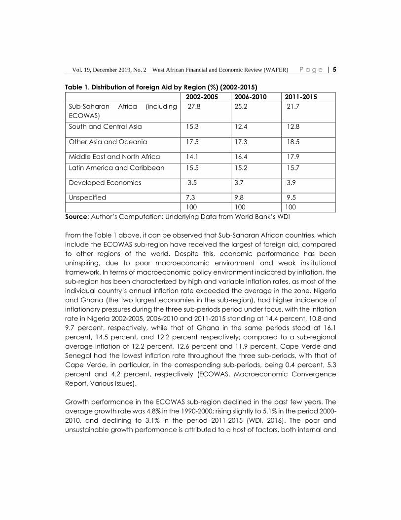
Table 1. Distribution of Foreign Aid by Region (%) (2002-2015)
Source: Author’s Computation: Underlying Data from World Bank’s WDI
From the Table 1 above, it can be observed that Sub-Saharan African countries, which
include the ECOWAS sub-region have received the largest of foreign aid, compared
to other regions of the world. Despite this, economic performance has been
uninspiring, due to poor macroeconomic environment and weak institutional
framework. In terms of macroeconomic policy environment indicated by inflation, the
sub-region has been characterized by high and variable inflation rates, as most of the
individual country’s annual inflation rate exceeded the average in the zone. Nigeria
and Ghana (the two largest economies in the sub-region), had higher incidence of
inflationary pressures during the three sub-periods period under focus, with the inflation
rate in Nigeria 2002-2005, 2006-2010 and 2011-2015 standing at 14.4 percent, 10.8 and
9.7 percent, respectively, while that of Ghana in the same periods stood at 16.1
percent, 14.5 percent, and 12.2 percent respectively; compared to a sub-regional
average inflation of 12.2 percent, 12.6 percent and 11.9 percent. Cape Verde and
Senegal had the lowest inflation rate throughout the three sub-periods, with that of
Cape Verde, in particular, in the corresponding sub-periods, being 0.4 percent, 5.3
percent and 4.2 percent, respectively (ECOWAS, Macroeconomic Convergence
Report, Various Issues).
Growth performance in the ECOWAS sub-region declined in the past few years. The
average growth rate was 4.8% in the 1990-2000; rising slightly to 5.1% in the period 2000-
2010, and declining to 3.1% in the period 2011-2015 (WDI, 2016). The poor and
unsustainable growth performance is attributed to a host of factors, both internal and
2002-2005 2006-2010 2011-2015
Sub-Saharan Africa (including
ECOWAS)
27.8 25.2 21.7
South and Central Asia 15.3 12.4 12.8
Other Asia and Oceania 17.5 17.3 18.5
Middle East and North Africa 14.1 16.4 17.9
Latin America and Caribbean 15.5 15.2 15.7
Developed Economies 3.5 3.7 3.9
Unspecified 7.3 9.8 9.5
100 100 100

6 | P a g e Hassan O. Ozekhome
external. The internal factors borders on poor domestic macroeconomic
management, leading to high and variable inflation, unemployment, stagnation and
rising fiscal deficits, corruption and poor governance. The external factors reflect the
increasingly hostile international economic environment, characterized by low and
falling primary commodity prices, resulting from negative external shocks, declining
terms of trade, and dwindling aid and capital flows into the region (Iyoha, 2004). Table
2 show the real GDP growth in ECOWAS countries in three sub-periods under focus.
Table 2: Growth Rate of Real GDP in ECOWAS
2002-2005 2006-2010 2011-2015
Benin 3.6 4.8 4.5
Burkina Faso 6.1 4.9 5.1
Cape Verde 5.2 6.8 7.1
Cote d’ Ivoire 0.1 2.9 5.2
The Gambia 5.6 6.5 5.6
Ghana 5.3 6.1 4.7
Guinea 2.7 3.3 3.2
Guinea Bissau 0.1 2.8 3.4
Liberia 1.1 8.9 5.5
Mali 5.1 4.9 4.9
Niger 4.3 4.8 4.8
Senegal 4.8 4.2 4.4
Nigeria 6.8 6.5 5.6
Sierra-Leone 8.6 6.2 5.5
Togo 2.1 2.6 2.6
Source: Author’s Computation Using Data from ECOWAS Central Banks and World
Economic Outlook
A cursory observation of Table 2 shows that most of the countries in the Sub-region
have had low and unsustainable growth pattern over three sub-periods, with the
exception of Cape Verde, Gambia, Ghana, Sierra- Leone and Nigeria, all member
countries of the West African Monetary Zone (WAMZ). Beginning from the latter part
of 2014 was a more testing economic period for the sub-region owing to pronounced
economic contraction in the ECOWAS region, particularly Nigeria (the largest
Vol. 19, December 2019, No. 2 West African Financial and Economic Review (WAFER) P a g e | 7
economy in the sub-region), due to internationally generated and transmitted shocks
from volatile primary commodity exports in the world market and exports instability; a
development which had negative reverberations in ECOWAS countries in terms of
economic and fiscal vacillations.
2.2 Institutional Quality
In this section, we show some stylized facts on the quality of institutions in the ECOWAS
sub- region using three institutional variables; control of corruption, rule of law and
political stability.
Control of Corruption
Corruption is the abuse of public office for self-gratification through fraudulent
activities especially siphoning, embezzlement and misappropriation of public funds
and is endemic in most ECOWAS countries (World Bank, 2016). Corruption has majorly
hampered growth trajectories in the sub-region and negatively affected aid
effectiveness. It weakens the ability to attract the much-needed external finance,
dislocates the productive system, and diminishes the incentive for creativity,
productivity and enterprise (Ozekhome, 2017). Most countries in the ECOWAS sub-
region have established anti-graft laws and institutions to curb the menace, like the
Economic and Financial Crimes Commission (EFCC) in Nigeria. Control of corruption,
therefore entails government commitment and transparency to fighting corruption
and the extent to which those found culpable are brought to face the law. It captures
the perceptions of the ability of the government to fight corruption to the barest
minimum through strong and effective institutional framework and rule of law and
procedures. Figure 1 shows the details of corruption control ranking in ECOWAS
countries.

8 | P a g e Hassan O. Ozekhome
Source: Eregha (2014)
Figure 1 above gives further credence to the trend of the ranking. The ranking is
between -2.5 to +2.5. It is evident from the figure that all the countries performed poorly
in the fight against corruption, except Cape Verde that performed better. The effect
of this is that government capacity to function effectively is reduced (Diop et al. 2010,
cited in Eregah, 2014), as it reduces the ability to attract and judiciously deploy
external finance resources (foreign aid in this context) for development purposes, as
expropriation, rent-seeking activities amongst others become prevalent.
Rule of Law
Another prominent institutional factor that has given rise to weak and negative effect
of aid on growth in the ECOWAS sub-region that has undermine growth and
development trajectory is the weak rule of law system. The rule of law (RL), as the
fulcrum of governance includes several measure of the degree to which citizens have
confidence in, and abide by the rules of society, and in particular, the independence,
effectiveness and predictability of the judiciary, the quality of contract enforcement,
property rights, the police, and the courts, as well as the likelihood of crime and
violence. Rule of law is based on a number of indicators measuring the supremacy of
the law, equality before the law, civil liberties and human rights, independence of the
judiciary and its effectiveness and predictability, and the enforceability of contracts
proceedings (World Bank, 2015). In a performance rating by the World Bank, the sub-
-1.5
-1
-0.5
0
0.5
12
00
0
20
02
20
03
20
04
20
05
20
06
20
07
20
08
20
09
20
10R
ank
Fig 1: Control of Corruption
Cote
Cape
Benin
Gambia
Guinea
Mali
Ghana
Niger
Nigeria
Vol. 19, December 2019, No. 2 West African Financial and Economic Review (WAFER) P a g e | 9
region performed poorly in many of the institutional variables. Using a range of (+2.5)
to –(2.5) , the sub region , except Cape Verde that consistently maintained an average
of -0.92 for regulatory quality, -1.20 for rule of law and -1.05 for government
effectiveness. Sound institutional reforms, which embed the rule of law, government
effectiveness and regulatory quality are thus required in the sub-region to make
foreign aid beneficial to growth, and drive economic growth to sustainable levels.
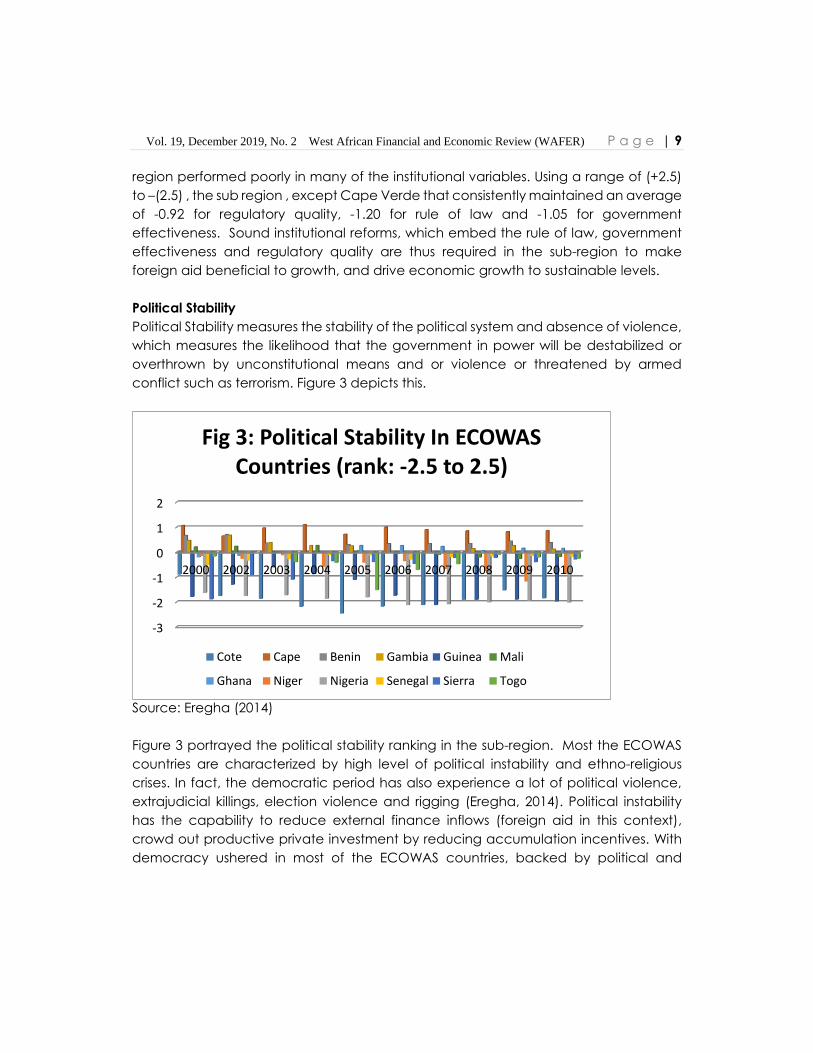
Political Stability
Political Stability measures the stability of the political system and absence of violence,
which measures the likelihood that the government in power will be destabilized or
overthrown by unconstitutional means and or violence or threatened by armed
conflict such as terrorism. Figure 3 depicts this.
Source: Eregha (2014)
Figure 3 portrayed the political stability ranking in the sub-region. Most the ECOWAS
countries are characterized by high level of political instability and ethno-religious
crises. In fact, the democratic period has also experience a lot of political violence,
extrajudicial killings, election violence and rigging (Eregha, 2014). Political instability
has the capability to reduce external finance inflows (foreign aid in this context),
crowd out productive private investment by reducing accumulation incentives. With
democracy ushered in most of the ECOWAS countries, backed by political and
-3
-2
-1
0
1
2
2000 2002 2003 2004 2005 2006 2007 2008 2009 2010
Fig 3: Political Stability In ECOWAS Countries (rank: -2.5 to 2.5)
Cote Cape Benin Gambia Guinea Mali
Ghana Niger Nigeria Senegal Sierra Togo
10 | P a g e Hassan O. Ozekhome
institutional reforms, democratic institutions are being strengthened and the regulatory
framework is being improved to enable external finance inflow affect growth
positively.
O, Connell and Soludo (1999) and Iyoha (2004) have argued that the diminishing aid
flows to African countries is attributable to poor macroeconomic policy environment,
donor fatigue, evidence of low aid effectiveness in many African countries, and
evidence of negative systemic effects of aid recipient countries. Other reasons
advance for the declining aid flows are absorptive capacity constraints, and that it
tends to crowd out domestic institutional developments and create rent-seeking
opportunities in African countries (Ozekhome, 2017). Similarly, Abuzeid (2012) posits
that aid also creates a moral hazard problem in the recipient country by serving as a
permanent soft budget constraint. The persistent influx of easy foreign aid money
creates the impression that the recipient government is always likely to be bailed out
when things go wrong. He maintained that foreign aid could affect governance and
growth through direct and indirect mechanisms. Through the direct mechanism, aid
can and does directly strengthen existing corruption patterns in contexts where high
levels of corruption are already rampant, if institutions are weak, and indirectly foreign
aid could harm governance and growth through its tendency to create multiple
distortions in the public sector, foster the emergence of a rentier state effect, and
delay pressures for effective reform.
3.0 REVIEW OF LITERATURE
3.1 Conceptual Issues
Foreign aid is often used synonymously with Official Development Assistance (ODA).
ODA is defined as the flow of official financing to the developing world that is
concessional in character, comprising of grants and loans with at least a 25 percent
grant component. It is generally administered with the objective of promoting the
economic development and welfare of developing countries, and comprises both
bilateral aid that flows directly from donor to recipient governments and multilateral
aid that is channelled through an intermediary lending institution like the World Bank.
This definition excludes debt relief, technical assistance, and other forms of aid
(Abuzeid, 2012). Official development assistance in the form of transfers constitutes an
important channel through which wealth is transferred from the rich developed nations
to the poor underdeveloped nations (Chatterjee and Turnosky, 2005). Net ODA is
defined as the sum of grants and net concessional loan disbursements for
development purposes less repayments, and includes free-standing technical
Vol. 19, December 2019, No. 2 West African Financial and Economic Review (WAFER) P a g e | 11
cooperation (TC) grants (Iyoha, 2004). Official development assistance to Africa,
including ECOWAS is provided mainly by the rich industrialized countries of Europe,
North America, Japan and Australia. These donors are members of the Development
Assistance Committee (DAC) of the Organization for Economic Cooperation and
Development (OECD). DAC countries are the source of official development
assistance to Africa and other developing countries.
In the narrow sense, aid consists of grants and technical assistance. A grant is transfer
of resources with no obligation for repayment. The grant may be in hard currency
(foreign exchange), services or kind. Technical assistance consists of men, capital and
technical equipment. More often than not technical assistance is designed to
promote capacity building in the recipient country through the training of manpower
and institution building. Nevertheless, in a wider sense, aid is often conceived to
include all transfer of resources. Thus, in addition to grants, aid encompasses loans and
private foreign investment. The loan, can be long-term, medium-term or short-term
and can have strings or conditionalities attached to it, just as grants. The key difference
between a grant and a loan is that a grant is a free gift, while the loan has to be repaid
(Iyoha, 2004). The justification for foreign aid according to Asher (1996) includes -
reconstruction of the economies of war military defence of the free world, and the
promotion of economic growth and political stability of the underdeveloped Africa.
3.2 Theoretical Literature
The theoretical underpinning for the proposition that aid can promote economic
growth is rooted in the two gap model (i.e- savings gap and foreign exchange gap)
articulated by McKinnon, (1964). According to the proposition, the savings gap arises
from the fact that domestic savings tend to be low in typical developing countries,
and thus falls short of required investment needed to drive economic growth, while
the foreign exchange gap arises from the fact that for variety of reasons to include;
extreme dependence on single or few range of primary commodity exports, export
instability, unfavourable terms of trade, and internationally generated and transmitted
shocks, many developing countries run import surpluses or balance of payment deficit
(Iyoha, 2004), leading to inadequate foreign exchange earnings needed to facilitate
the import of the required capital machineries and other inputs needed for growth.
Thus, these gaps can be filled by foreign capital inflow in the form of aid (Ozekhome,
2017).
In addition, there exist two strands of literature on the role of foreign aid on economic
growth. The first proponents- the Modernisation Hypothesis asserts that foreign capital
12 | P a g e Hassan O. Ozekhome
inflow is necessary and sufficient for economic growth in the less developed countries.
They argue that there exists a positive relationship between aid and economic growth
because it complements domestic resources and also supplements domestic savings.
Furthermore, foreign aid assists in closing the foreign exchange gap, provides access
to modern technology and managerial skills, and allows easier access to foreign
market (Chenery and Strout, 1966; Levy, 1988; Islam, 1992). The second proponents
argue that external capital in the form of aid exerts significant negative effects on the
economic growth of recipient countries. According to this view, foreign aid is fully
consumed and substitutes rather than compliments domestic resources. Furthermore,
foreign aid assists to import inappropriate technology, distorts domestic income
distribution, and encourages a bigger, inefficient and corrupt government in
developing countries (Boone, 1994; 1996; Easterly, 1999). They argue that the host
country tend to depend on aid (aid dependency-syndrome) and its poor linkages
within the economy to the detriment of meaningful and productive domestic
investment. This situation has the tendency to create destabilizing effects on growth,
especially when aid is withdrawn or reversed (Bornscier, 1980). They further maintained
that as a result of diversion of aid from investment to unproductive consumption uses,
corruption tend to increase in host countries, thereby lowering growth.
The literature on the role of foreign private capital inflow however contains
overwhelming evidence in support of the growth-enhancing effects of aid, particularly
in the presence of sound macroeconomic policy environment, good institutional
framework and effective governance. In the same vein, recent developments in
growth theory argue that improvements in technology, efficiency, capital
accumulation and productivity brought about by foreign private capital (aid in this
context) have the capacity to stimulate growth. The theoretical contention is based
on the notion that aid increases the rate of technical progress in the host country
through its positive spillovers from advanced technology, managerial expertise,
entrepreneurship, and innovation (Morrissey, 2001).
3.3 Review of Empirical Studies
Different approaches have been used to analyze growth models to foreign aid,
macroeconomic policy and institutional quality. Studies focusing on single country
analyses, although few have adopted univariate models (see Chatterjee, & Turnosky,
2005; Dalgaard, Hasen, & Tarp, 2004), multivariate model (see Feeny, & McGillivray
(2008 and Sakyi, 2010) and simultaneous equations model (Dollar & Easterly; 1999,
Gounder, 2001). For studies that utilize panel data, the static model estimators involving
fixed effects and random effects are evident (see Dhakal, Upadhyaya, & Upadhyaya,
Vol. 19, December 2019, No. 2 West African Financial and Economic Review (WAFER) P a g e | 13
1996; Burnside and Dollar, 2000; Gomannee, Girma & Morrissey , 2002; Iyoha, 2004;
Ericsson and Irandoust, 2005; Hatemi-J & Irandoust, 2005; Kasuga, 2007; Cieslik and
Tarsalewska, 2008; Ndambendia & Njoupouognigni, 2010; Malik, 2010; Eregha, Sede &
Ibidapo, 2012; Ekanayake, & Chatrna, 2012; and Olabode, 2013), while the dynamic
model estimators involving the GMM-type seem to have gained prominence (e.g
Veiderpass and Andersson (2007); hence, the choice of the latter in the current study.
Some of the attractions to the GMM-type estimators, including the underlying
assumptions are well-documented in the studies of Ndambendia and Njoupouognigni,
(2010), Tiwari (2011); Fiodenji & Evlo, (2013; Ozekhome, (2017). In addition, this category
of estimators require short T, which is one of the features of data on aid and institutional
quality (see Fiodendji & Evlo, 2013). These variables are rarely available for a longer
time horizon, and that partly explains why most studies use panel with several cross-
sections to compensate for the short time series.
As observed by the previous studies, the effect of foreign private capital inflow (aid in
this respect) on economic growth is positive and statistically significant (Roy and Berg,
2006; Xu and Wang, 2007; Bhandari et al., 2007). The effect has been found to be
supported by some institutional factors such as level of education, basic physical
infrastructure, and appropriateness of institutions (Adams, 2008). However,
attractiveness of aid which is based on good policy, economic and political stability
of host country is a necessary condition, but not sufficient to stimulate positive
relationship between aid and economic growth. Concerning the channels, it seems
obvious that domestic investment is likely the most important in which private capital
exerts a strong positive effect on economic growth in developing countries. Some
other studies find that good fiscal, monetary and trade policies as well as right
institutional framework are a necessary condition for effectiveness in the foreign aid-
growth nexus (Ekanayake and Chatrna, 2012; Fiodenji and Evlo, 2013). Olabode (2013)
re-examines the effects of disaggregated foreign aid on poverty level in 8 West African
countries between 1975 and 2010. Employing both the techniques of heterogeneous
panel unit root test, cointegration test and empirical estimators with heterogeneous
slopes, the findings reveal that total foreign aid impact positively on poverty, while
technical aid reduces poverty.
Fiodendji and Evlo (2013) in particular, examine the threshold effects in the foreign aid-
economic growth nexus using institutional quality and macroeconomic policy
environment. Employing a modified panel threshold model on panel data of 13
ECOWAS countries over the period 1984 to 2010, the findings show that the relationship
between aid and economic growth is nonlinear with a unique threshold of 0.206. The
14 | P a g e Hassan O. Ozekhome
evidence further show that stable macroeconomic environment and good
institutional framework are indispensable for aid effectiveness in ECOWAS countries
since bad institutional quality may have detrimental effects on economic growth. The
study identified the conditions under which aid has a positive impact on economic
growth which include: the combination of macroeconomic policy environment and
institutional quality above their thresholds respectively. This according to them, is
relevant for the achievement of sustainable economic growth. The authors conclude
that the findings will be important for policymakers and international financial
institutions which increasingly favour conditionality and selectivity in the allocation of
aid resources. The major policy implication of the findings according to the authors is
not that foreign aid should be reduce, but rather a call for rethinking strategies for
international assistance and redesigning existing aid programmes.
From the fairly large volume of literature, there is paucity of empirical studies on the
effects of aid on growth, accounting for macroeconomic policy environment and
institutional quality, using dynamic panel estimators, hence, warranting further
empirical investigations.
4.0 METHODOLOGY
4.1. Theoretical Framework and Model Specification
The empirical model used in this study is motivated by the endogenous growth model.
The most interesting aspect of endogenous growth models is that it helps to explain
the disparities in growth rate across countries, arising from differential rates of capital
accumulation (i.e domestic and external capital in this context), institutional quality
and macroeconomic environment.
The general endogenous production function is
Y = AK i L1-i (1)
Where:
A = Total factor productivity- a measure of efficiency of factor inputs
K = Capital stock (which is decomposed to into human and physical capital)
L = Labour.
α and β, represents the elasticity of output with respect to capital and labour,
respectively.
The model in equation (1) is an endogenous growth model since the residual
component, A, which is a measure of technological progress and human capital
accumulation are endogenized; thus, implying that technological knowledge and the

Vol. 19, December 2019, No. 2 West African Financial and Economic Review (WAFER) P a g e | 15
accumulation of human capital are incorporated not as exogenous growth-
generating factors but explaining the growth process itself.
Following Jones [1998], the aggregate production function is provided:
Y= IKα(AL)1- α (2)
Where, Y= Real output (ie as real GDP (a measure of economic growth), I denotes the
influence of an economy’s infrastructure on the productivity of its inputs, K is capital,
decomposed to into human and physical capital, A is a measure of technology, (i.e
total factor productivity or a measure of efficiency of factor inputs), L is labour stock;
α and 1- α (i.e β), represent the elasticity of output with respect to capital and labour,
respectively, where α is a parameter between 0 and 1. In contrast to Solow and
neoclassical models of growth, in endogenous growth models, changes in the rate of
investment and changes in government policies can impact on the long run rate of
growth. This model suggests that the infrastructure of an economy (I), relating to the
government policies and institutions which make up the economic environment, is an
important determinant of growth. Jones (1998) suggested that the cost of setting up
businesses and the ability of investors to reap returns from their investments, varies
considerably across countries. Thus, an important assumption in this specification is that
institutions and government policies are considered to affect growth through two
channels, the total factor productivity and the investment channels. A large part of
this variation arises from differences in government policies and institutions – referred
to as the infrastructure of a country. He predicts that a country that attracts
investments in the form of capital for businesses, technology transfer from abroad and
skills of individuals will be one in which: (a) the institutions and laws favour production
over diversion; (b) the economy is open to international trade and competition in the
global marketplace; and (c) the economic institutions are stable. Jones (1998, cited in
Eregha, Sede & Ibidapo, 2012) states that a good infrastructure provides an
environment which encourages investment, the acquisition of skills, invention and
technology transfer. The empirical model motivated by the above theoretical
considerations takes the stylized extended (modified) aid-growth function.
yit = f (AID, I, X) (3)
Where yit is the dependent variable, which is the growth rate of real GDP (GRGDP)- a
measure of economic growth, I , is a measure of infrastructure (encompassing
macroeconomic policy and institutional quality), X is a vector of other
macroeconomic control variables, which according to literature influences the aid
growth nexus. This is because aid can only contribute significantly to growth through
increase capital stock, improvements in human capital (i.e investment in human and
physical capital) and other policy variables. In particular, good macroeconomic
policy and institutional quality enhances aid effectiveness. The inclusion of these

16 | P a g e Hassan O. Ozekhome
variables is to include, as much as possible other critical variables that impact on the
assumed relationship, and thus avoid omitted variable bias.
These variables thus include;
OPN = Openness of the domestic economy
SCHL = enrolment in secondary school as a measure of human capital accumulation
INV= real gross domestic capital formation to GDP (percent)
INST=institutional quality measured by averaging the six indicators of institutional quality
to include rule of law, accountability, government effectiveness, control of corruption,
regulatory quality and political stability
INF=Inflation rate (a measure of macroeconomic environment). As an indicator of
macroeconomic environment, the inflation rate assumes greater importance, and it
reflects the overall ability of a government to manage the economy.
The empirical specification of the model to be estimated, without the interaction terms
is:
yi t=, α0 + α1OPNi,t+ α2AID,t+ α3INVi,t+ α4SCHi,t+ α5INFi,t + α6INST (4)
The extended model is further expanded to include three interaction terms to capture
the influence of institutional quality and macroeconomic policy environment on the
effectiveness of aid on growth. Doing this leads to the following interaction model:
yi t=, α0 + α1OPNi,t+ α2AIDi,t+ α3INVi,t+ α4SCHi,t+ α5INFi,t + α6INST + α7AID*INFi,t
+ α8AID *INSTi,t + α9INST*INFi,t + εt (5)
Where AID*INST, AID*INF, INST*INF = interaction of aid and institution, aid and
macroeconomic policy environment, and institutional quality and macroeconomic
policy environment, respectively, i represent country (The 15 ECOWAS, and t represents
the period (2002-2015). All other variables are as previously defined.
The a priori expectations are (α1, α2 α3, α4, α6, α7, α8, α9) > 0; α5 < 0.
α0 – α9 are parameters to be estimated and εt is the unobserved error term.
From macroeconomic theory, aid, openness, foreign direct investment, real domestic
capital formation, human capital and interaction term consisting of aid interacted
with institutional quality variable and macroeconomic policy are expected to have
positive impact on economic growth, while the coefficient of inflation is expected to
Vol. 19, December 2019, No. 2 West African Financial and Economic Review (WAFER) P a g e | 17
have a negative relationship with economic growth. The expected signs are based on
capital accumulation and external finance theory. The higher degree of trade
openness of a country, the higher will be the economic growth rate since trade
openness facilitates greater integration into the global economy and stimulates
growth through the channels of better resource allocation, greater competition,
innovation, transfer of technology and access to foreign capital. Foreign aid stimulates
growth by increasing the stock of capital, easing domestic resource and foreign
exchange constraints to development, and facilitating the transfer of advanced
technology, managerial and technical know-how from industrialized countries to host
countries, thereby increasing productivity through positive spillovers, which in turn
stimulates growth.
The higher the level of domestic investment, the more rapid will be the rate of
economic growth since investment increases the capital stock and stimulate
aggregate demand. An improvement in human capital brought about by human
capital accumulation enhances economic growth through increase in the
productivity of the work force. Thus, the higher the quality of human capital, the higher
the rate of economic growth. Strong institutional framework that guarantees
regulatory quality, government effectiveness, combats corruption and rent-seeking
behaviour of economic agent is expected to impact positively on growth and
enhance the effectiveness of aid. The interaction of aid with macroeconomic policy
variable and aid with institutional quality variable is thus theoretically expected to
have a positive relationship with economic growth. This is because; sound
macroeconomic policy environment and institutional framework enhance aid
effectiveness on growth.
4.2 Definition of Variables and Sources of Data
The definitions of the variables in the model, as well as the sources of data are provided
in Table 3.

18 | P a g e Hassan O. Ozekhome
Table 3. Definition of Variables and Data Sources
Variable Description Source
Growth rate
of real GDP
Annual real GDP growth
World Economic
Outlook (IMF), WAMZ
Macroeconomic
Convergence Report
Trade
Openness
Sum of Imports and exports as
percentage of GDP
World Development
Indicators (World Bank)
AID Ratio of foreign aid (Official
Development Assistance) to GDP
percent
World Development
Indicators (World Bank)
Investment Ratio of gross capital formation to GDP
percent
World Economic
Outlook (IMF
Human
capital
Secondary school enrolment ratio World Development
Indicators (World Bank)
Institutional
quality
Institutional quality is measured as the
average of six institutional indicators
http://info.worldbank.org/governance/
wgi/index #home
World Development
Indicators (World Bank)
Inflation Annual growth rate of consumer price
index
WAMZ Macroeconomic
Convergence
Source: Author’s compilation
4.3 Justification for the Inclusion of the Control variables
Several control variables are critical to the effectiveness of aid on growth. First,
institutional quality and government policies (proxied by macroeconomic policy
influence aid effectiveness in line with the endogenous growth theory that strong
policy variables and institutional quality are critical determinants of growth, as well as
influencing the effect of external private capital (aid in this context). Thus, the inclusion
of macroeconomic policy, institutional quality variable and trade openness is in line
with the extant of theory.
Second, domestic investment influences the absorptive capacity of foreign private
capital. As stock of capital increases, the rate of growth increases as well, as
accumulation of human and physical capital are critical to sustained economic
growth in the long run, since they facilitate the efficient absorption of new capital
development, improves the speed of adaptation of entrepreneurs and generates

Vol. 19, December 2019, No. 2 West African Financial and Economic Review (WAFER) P a g e | 19
innovation necessary for sustained economic growth. In particular, increase level of
domestic investment, will generate more rapid economic growth since investment
increases the capital stock and stimulate aggregate demand. Human capital
accumulation, in accordance with the endogenous growth model, permits diffusion
of knowledge (knowledge spillovers), technology efficiency and productivity growth,
which have the capacity to stimulate growth. Through ‘learning by doing’, the model
further demonstrates the high growth-generating capacity of human capital
accumulation. In general, the model demonstrates that human capital accumulation
encompassing knowledge and skills which induce labour efficiency is critical to rapid
and sustained growth path. This position is supported by Lucas (1988) who argued that
increased investment and improvements in innovations and technical progress arising
from human capital development can lead to increase productivity and
competitiveness, which trigger a further growth. The inclusion of the variables is thus in
line with theory and extant literature.
4.4 Estimation Technique
The choice of a GMM-type is based on a number of reasons. First, the GMM-type
estimators including the system GMM estimator are used for dynamic models as they
help resolve any inherent endogeneity in the model. Second, the GMM-type
estimators are also useful when dealing with a situation where N>T, I presumed to be
the case here. Third, the estimators are used if T is short (where T<25) after accounting
for the first and second conditions.
One of the problems of most studies of the aid-growth relationship based on cross-
country regressions is that they lump together countries of heterogeneous
characteristics and size. There is also the problem of reverse causality. For example,
aid may rise in response to poor growth (and saving) performance, producing a high
correlation between low growth and high aid flows. This may generate potential bias
in estimation. In order to avoid the problems of potential bias and heteroskedasticity
arising from endogeneity (simulataneity) associated with cross-country studies, and
problems of mis-specification and omission of variable bias, this study adopts the
system-GMM. The technique addresses the triple-problem of endogeneity of the
regressors, the measurement error and omitted variables. In the literature, one of the
methods of estimating a dynamic panel data model is the first-differenced equation
estimated by the Generalized Method of Moments (GMM) approach. This approach
overcomes the problem of unobserved period and country specific effects (economic
peculiarities) and joint endogeneity of most of the explanatory variables with the
endogenous variable, and, thus, control for the biases resulting from simultaneous or

20 | P a g e Hassan O. Ozekhome
reverse causation. The system-GMM estimator developed by Arellano and Bover
(1995), Blundell and Bond (1998) tends to have better finite sample properties, provide
more precise, less biased, consistent estimates and asymptotically efficient estimates
than the first-differenced GMM estimator since it exploits the available time-series
information more efficiently; Blundell and Bond (1998), and Bond et al. (2001).
The good performance of the System GMM estimator relative to the difference-GMM
estimator in terms of finite sample bias and root mean square error has made it
preferable, particularly when series are persistent and there is asymptotic reduction in
the finite sample bias due to the exploitation of additional moment conditions (Alonso-
Borrego and Arellano, 1999). The system GMM estimator is computed by combining
moment conditions for the equations in first-differences using suitably lagged variables
as instruments, with additional moment conditions for the equations in levels where the
instruments are suitably lagged values, provided these first-differences are
uncorrelated with the within-sample effects. System GMM estimator thus eliminates
any potential bias that may arise from ignoring dynamic endogeneity and also
provides theoretically based and powerful instruments that accounts for simultaneity
while eliminating any unobservable heterogeneity (Blundell and Bond (1998). Unlike
the difference estimation, the system estimators make use of lagged differences of the
endogenous variables as standard instruments for the level equation. In view of the
obvious strengths of the Blundell and Bond’s (1998) extended version of the GMM
estimator (known as the System- GMM estimator) in overcoming complications that
may arise from efforts to estimate the usual linear dynamic panel data models; it is
therefore considered appropriate and applied in this study. To check for the robustness
of the estimated parameters, the Fully Modified Ordinary Least Squares (FMOLS), which
corrects for autocorrelation, potential endogeneity of regressors and reverse
cauasality is also employed to estimate the model. The FMOLS is also able to account
for considerable heterogeneity across individual panel to produce asymptotic
unbiased estimators and nuisance parameters, free normal distributions (Pedroni,
2000).
5.0 EMPIRICAL RESULTS
5.1 Descriptive Statistics
Table 4 presents the summary statistics for the variables used in this study. Average real
GDP growth for the ECOWAS countries during the period is 4.9 percent. The median
value is 5.1 percent. The maximum and minimum growth rate is 8.2 percent and 0.8
percent respectively. Invariably, growth performance tend to have converged
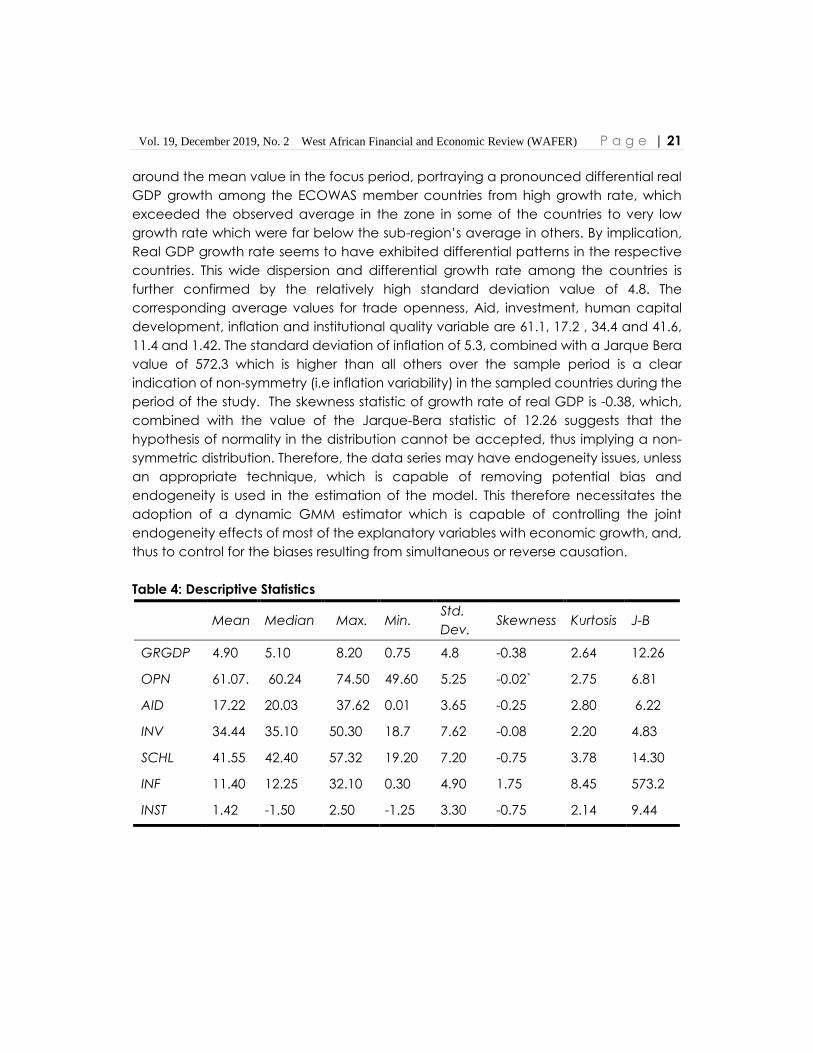
Vol. 19, December 2019, No. 2 West African Financial and Economic Review (WAFER) P a g e | 21
around the mean value in the focus period, portraying a pronounced differential real
GDP growth among the ECOWAS member countries from high growth rate, which
exceeded the observed average in the zone in some of the countries to very low
growth rate which were far below the sub-region’s average in others. By implication,
Real GDP growth rate seems to have exhibited differential patterns in the respective
countries. This wide dispersion and differential growth rate among the countries is
further confirmed by the relatively high standard deviation value of 4.8. The
corresponding average values for trade openness, Aid, investment, human capital
development, inflation and institutional quality variable are 61.1, 17.2 , 34.4 and 41.6,
11.4 and 1.42. The standard deviation of inflation of 5.3, combined with a Jarque Bera
value of 572.3 which is higher than all others over the sample period is a clear
indication of non-symmetry (i.e inflation variability) in the sampled countries during the
period of the study. The skewness statistic of growth rate of real GDP is -0.38, which,
combined with the value of the Jarque-Bera statistic of 12.26 suggests that the
hypothesis of normality in the distribution cannot be accepted, thus implying a non-
symmetric distribution. Therefore, the data series may have endogeneity issues, unless
an appropriate technique, which is capable of removing potential bias and
endogeneity is used in the estimation of the model. This therefore necessitates the
adoption of a dynamic GMM estimator which is capable of controlling the joint
endogeneity effects of most of the explanatory variables with economic growth, and,
thus to control for the biases resulting from simultaneous or reverse causation.
Table 4: Descriptive Statistics
Mean Median Max. Min. Std.
Dev. Skewness Kurtosis J-B
GRGDP 4.90 5.10 8.20 0.75 4.8 -0.38 2.64 12.26
OPN 61.07. 60.24 74.50 49.60 5.25 -0.02` 2.75 6.81
AID 17.22 20.03 37.62 0.01 3.65 -0.25 2.80 6.22
INV 34.44 35.10 50.30 18.7 7.62 -0.08 2.20 4.83
SCHL 41.55 42.40 57.32 19.20 7.20 -0.75 3.78 14.30
INF 11.40 12.25 32.10 0.30 4.90 1.75 8.45 573.2
INST 1.42 -1.50 2.50 -1.25 3.30 -0.75 2.14 9.44
22 | P a g e Hassan O. Ozekhome
5.2 Analysis of Generalized Method of Moments (GMM) Results
The Arellano and Bond (1991) GMM estimator can be carried out to determine the
impact of foreign aid on economic growth in ECOWAS. The growth model is estimated
first without accounting for macroeconomic policy environment and institutional
quality and then, accounting for their respective interaction with aid (i.e without the
inclusion of the interaction of aid with institutional quality and aid with macroeconomic
policy and with their inclusion The alternative results from the FMOLS which is used to
test for robustness, by using alternative proxies for the institutional quality variable is also
presented.
Lagged growth rate of real GDP has the correct sign and is significant at the 10 percent
level in all the estimations. This implies that previous economic growth constitute a basis
for attaining higher economic growth rate in countries. This is particular important as it
tends to help in the re-direction of macroeconomic policies towards achieving better
growth rate in succeeding years. Basing the elasticity estimate on the interaction
model, a 10 percent increase in previous economic growth will stimulate future
economic growth in the succeeding year by 0.8 percent. The coefficient of trade
openness is consistent with theoretical projection in all the model estimations and
significant at the 1 percent level. Thus, increased trade openness stimulates economic
growth in ECOWAS countries through more integration into the global economy,
efficient and optimal resource allocation and competition. The finding supports the
results of Adamu, Igodaro and Iyoha (2012) and Ozekhome (2017). In line with the
estimates, a 10 percent increase in trade openness will stimulate economic growth by
2.1 percent in ECOWAS countries.
The coefficient of foreign aid is negative and fails the significance test in the model
without the pair of interaction. Invariably, in the absence of good institutions and
macroeconomic environment, aid effectiveness on growth is negative and weak. The
interaction of aid with macroeconomic policy and institutional quality with
macroeconomic policy are both positive, but pass the significance test only at the 10
percent level, while that of the interaction of aid with institutional quality is statistically
significant at the 5 percent level. This implies that strong institutional framework that
encompasses government effectiveness, regulatory quality, rule of law, political
stability, enforceability of contract proceedings, prevention of expropriation and rent-
seeking behaviours matters more to aid effectiveness than macroeconomic policy, in
terms of moderating the negative impact of aid on growth in ECOWAS countries, and
making aid beneficial to growth. Apparently, the latter enhances the former, as it
provides strong institutional settings for good economic policy management. Thus,

Vol. 19, December 2019, No. 2 West African Financial and Economic Review (WAFER) P a g e | 23
sound macroeconomic policy environment and good institutional framework are
critical to aid effectiveness on growth in the sub-region, but building strong institutional
framework is more compelling and result-oriented. The finding corroborates the results
of Abuzeid (2012) and Fiodendji and Evlo (2013).
Thus, aid effectiveness in ECOWAS countries can be enhanced through sound and
stable macroeconomic policies, good institutional framework, excellent economic
management and good governance. This idea is also consistent with the insight that
countries with lower level of distortions, good macroeconomic policies and institutional
framework, will on the average grow faster than countries with poor macroeconomic
and institutional environment. Aid effectiveness is thus responsive to sound
macroeconomic policy environment, good institutions and efficient economic
management. The elasticity coefficient of the interaction of aid with macroeconomic
policy, aid with institutional quality and institutional quality with macroeconomic policy
show a growth intensification of 0.6 percent, 0.2 percent and 0.1 percent, respectively.
Invariably, sound economic policy management, good governance and quality
institutional framework enhance growth effectiveness of aid.
The coefficient of domestic investment (real gross domestic capital formation) has the
expected positive sign and is significant at the 1 percent level in all the estimations.
This implies that increase investment in capital is highly growth-inducing. Invariably,
increased capital accumulation has the capacity to generate faster economic
growth in the sub-region. The elasticity coefficient of gross capital formation (domestic
investment) shows that a 10 percent increase in domestic capital accumulation will on
the average trigger economic growth in ECOWAS region by 2.3 percent.
The coefficient of human capital is appropriately signed in line with theoretical
expectation and passes the significance test at the 5 percent level in all the
estimations. Thus, increase human capital development will promote rapid economic
growth in ECOWAS countries, through the acquisition of better knowledge that
induces the speed of technological adaptation, via its positive spillovers, labour
productivity, efficient absorption of new capital developments, improved managerial
enterprise and generation of innovation necessary for growth (Baliamount-Lutz, 2004;
Ozekhome, 2017). The elasticity coefficient indicates that a 10 percent increase in
human capital accumulation (development) will on the average induce economic
growth in ECOWAS by 2.2 percent.

24 | P a g e Hassan O. Ozekhome
The coefficient of institutions is positively signed but not significant at conventional
levels in all the estimations. This implies that though institutions positively affect growth,
the sub-region is characterized by weak institutional framework. The result buttresses
the findings of Park (2012) and Ozekhome (2016) and again confirms the earlier
findings that in the absence of interaction, the impact of institutions on growth is weak
in the sub-region, but when interacted with aid, growth is enhanced.
Inflation (an indicator of macroeconomic environment) is negatively signed in line with
theoretical expectation, and is statistically significant at the 5 percent in all the
estimations. Thus, high inflation (a symptom of macroeconomic instability) undermines
economic growth in the sub-region. The elasticity coefficient indicates that a 10
percent rise in the rate of inflation will dampen economic growth in ECOWAS by
percent 1.8 percent.
Considering key diagnostic tests for the robustness and validity of results obtained, the
Hansen-J over-identification test, which serves to verify the validity of instruments fails
to reject the null hypothesis that there is no endogeneity problem in the two GMM-
type estimations. This implies that the over-identifying restrictions are equal to zero and
valid. Thus, we cannot reject the specification of the model, since it is well specified
and the instruments seem to be appropriate and valid. The result provides good
certification for the choice of the exogeneity of the levels and differenced instruments,
as required in a system-GMM. The post-estimation evidence also leads to the rejection
of the null hypothesis of no serial correlation at order one in the first-difference errors,
but a failure to reject same at order two (with AR (1) = -2.88 (0.003)*** and AR (2) =
-0.65 (0.51) and AR (1) = -3.01 (0.003) *** and AR (2) = -0.61 (0.54), respectively for the
model without interaction and with interaction. There is thus no evidence to invalidate
the model considering that, according to Arellano and Bond (1991), the GMM
estimates are robust in the presence of first-order serial correlation, but not in the
second-order serial correlation in the error terms. The long-run variance in the
alternative FMOLS estimation used for robustness check also indicates that the model
is robust and sound. This therefore implies both models are good for structural and
policy analysis.

Vol. 19, December 2019, No. 2 West African Financial and Economic Review (WAFER) P a g e | 25
Table 5. Results from the Arellano and Bover (1995) (GMM) Estimator
The Effect of Aid on Growth in ECOWAS
Regressors Without
Interaction
With
(Interaction)
FMOLS
C 0.892 0.125* -
S.E 0.015 0.107
Lagged GRGDP 0.8024* 0.076* -0.773*
S.E 0.002 0.104
OPN 0.314*** 0.213*** 0.356***
S.E 0.070 0.051
AID -0.113 -0.016 -0.093
S.E 0.104 0.102
INST 0.019 0.046 0.031
S.E 0.105 0.103
INF -0.109** -0.177** -0.126**
S.E 0.020 0.003
AID*INF 0.061 0.032
S.E 0.033 0.029
AID*INST 0.024** 0.003**
S.E 0.024 0.018
INST*INF 0.011* 0.016*
S.E 0.0041 0.038
INV 0.202*** 0.225*** 0.049***
S.E 0.202 0.196
SCHL 0.1320*** 0.223** 0.170**
S.E 0.602 0.014
J statistic 3.60 4.025
AR(1)
AR(2)
-2.880[0.004]
-0.652[0.51]
-3.01[0.003]
-0.610[0.54]
Long-run Variance 0.032

26 | P a g e Hassan O. Ozekhome
Reported coefficients and corresponding standard errors (S.E.) in the interaction model
estimation are average marginal effects and have been calculated following the
approach suggested by Bartus (2005).
*** Statistical significance at the 1% level: ** Statistical significance at the 5 % level; *
Statistical significance at the 10% level
Note: Sargan, Hansen tests, AR (1) indicates rejection of the null hypothesis of no serial
correlation at order one (1) and non-rejection of same at order two (2) AR (2).
Source: Author’ computation
6.0 CONCLUSION
This study investigates the impact of foreign aid on economic growth, and whether
macroeconomic policy environment and institutional settings matter to the to aid
effectiveness in the ECOWAS region, using system-GMM on dynamic panel data for
the period 2002-2015. In doing this, a growth model that does not account for
macroeconomic policy environment and institutional quality (i. e without their
interaction with aid) is first estimated, and then, estimating another, where they are
accounted for, using pairs of interaction of variables. The empirical results reveal that
foreign aid has a negative but weak impact on growth in the model where
macroeconomic policy environment and institutional quality are not accounted for.
But when macroeconomic policy environment (poxied by inflation) and institutional
quality variable are accounted for (i.e interaction of aid with macroeconomic policy
environment and interaction of aid with institutional quality), the negative effect of aid
is moderated, with the coefficient of the interactive terms appearing positive and
significant, with that of the interaction of aid and institutional quality more
pronounced. This implies that although macroeconomic policy environment and
institutional quality both matter for aid effectiveness, greater emphasis should be
placed on creating strong institutional framework in terms of rule of law, political
stability, control of corruption, government effectiveness, regulatory framework and
curtailment of rent-seeking and expropriational tendencies.
The interaction of institutional quality with macroeconomic policy environment also
yields positive and significant effect on economic growth. The intuition and implication
of this finding is that sound policy and good economic management and institutional
setup are critical to enhancing aid effectiveness. As the evidence show, without good
institutions and favourable macroeconomic policies, given the poor macroeconomic
policy environment and institutional framework in the sub-region, aid is likely to have a
detrimental impact on growth. Ostensibly, selectivity on the basis of institutional setups
that promote good governance and macroeconomic policy management could

Vol. 19, December 2019, No. 2 West African Financial and Economic Review (WAFER) P a g e | 27
become potential policy conditonalities for official development assistance by donors.
Other variables that influence economic growth in the region are openness to trade,
real gross domestic capital formation and human capital development.
Against the backdrop of making aid and other private capital inflows beneficial to
growth in the sub-region, in terms of effectiveness, it is important that sound and stable
macroeconomic policy environment and good institutional structures be put in place
in the sub-region. In addition, economic openness to trade, increase investments in
physical and human capital accumulation are critical to sustained economic growth
in the sub-region. Nevertheless, cautious optimism should be exercised in terms of over-
dependence on foreign aid, a condition termed ‘aid dependency syndrome’, in
which after large injections of aid for many years, a country or region becomes too
dependent on aid and no longer prepares to be self-reliant. Given sudden policy
reversal culminating in abrupt aid withdrawal by donors, such country or region might
be heavily affected, in addition to sometimes ‘too stringent’ and unfavourable
economic conditionalites that may be attached to receiving aid form bilateral donors.
28 | P a g e Hassan O. Ozekhome
References
Abuzeid, A. (2012). Foreign aid and the Big-Push theory: Lessons or Sub-Saharan Africa,
Stanford Journal of International Relations, 11 (1), 16-23.
Adamu, P. A., Ighodaro, C.A. & Iyoha, M.A. (2012). Trade, foreign direct investment
and economic growth: Evidence from the countries of the West African
Monetary Zone. The West African Economic Review, 1(2), 10-31.
Alesina, A., & Weder, B. (2002). Do corrupt governments receive less? The American
Economic Review, 92 (4), 1126-1137.
Arellano, M., & Bond, S., (1991). Some tests of specification for panel data: Monte Carlo
Evidence and an application to employment equations. Review of Economic
Studies, Wiley Blackwell, 58(2), 277-97, April.
Arellano, M., & Bover, S., (1995). Another look at the instrumental variable estimation of
error-components models. Journal of Econometrics, 68, 29-51.
Asher, R.E (1966). Grants, loan and local currencies: Their role in foreign aid.
Washington D.C. The Brookings Institute.
Baliamoune – Lutz, M. & Ndikumana, L. (2007). The growth effects of openness to trade
and the role of institution: New evidence from African countries working paper
N0 2007-05. Department of economics, University of Massachusetts, Amherst,
February.
Bartus, T. (2005). Estimation of marginal effects using margeff. Stata Journal, 5(3).
Bhandari, R., Dhakal D., Pradhan G., Upadhyaya K. (2007). “Foreign aid, FDI and
economic growth in East
European countries”. Economics Bulletin, 6, (13), 1-9
Boone, P. (1994). The impact of foreign aid on savings and growth. Center for
Economic Performance, Working Paper 1265, London.
Boone, P (1996). Politics and effectiveness of aid. European Economic Review, 40, 289-
329.
Bowles, P. (1987). Foreign aid and domestic savings in less developed countries: some
tests for causality. World Development 15(6), 789-796.
Bornschier, V. (1980). Multinational corporations and economic growth: A cross-
national test of the decapitalization thesis. Journal of Development Economics,
7, 59.71
Burnside, C. & Dollar, D. (2000). Aid, policies, and growth. American Economic Review,
90,847–868.
Burnside, C., &Dollar, D. (1997). “Aid, policies, and growth”. Policy research Working
Paper 1777. Washington,
DC: World Bank.

Vol. 19, December 2019, No. 2 West African Financial and Economic Review (WAFER) P a g e | 29
Chatterjee, S and Turnosky, S.J. (2005). Foreign Aid and economic growth: The role of
flexible labour supply. A Paper Presented at the Annual Conference of the
royal Economic Society in Swansea.
Chenery, H.B., & Strout, A. (1966). Foreign assistance and economic development.
American Economic Review 56, 679-733.
Ciselik, A, & T arsalewska, M. (2008). Trade, foreign direct investment and economic
growth: Empirical evidence from CEE
countries.www.etsg.org/ETSG2008/Papers/Ciestlik.
Collier, P. and Dollar, D. (2002). Aid Allocation and poverty reduction. European
Economic Review, 46, 1475–1500.
Dalgaard, C, Hasen, H & Tarp, F. (2004). On the empirics of foreign aid and Growth.
The Economic Journal, 114, F191-F216.
De Gregorio, J. (1992). Economic growth in Latin America. Journal of Development
Economics, 39(1), 59-84.
Dhakal, D., K. Upadhyaya, & M. Upadhyaya (1996). Foreign aid, economic growth and
causality. Rivista Internazionale di Scienze Economiche Commerciali. 43: 597-
606.
Diop, A., G. Dufrenot and G. Sanon (2010), ‘Is Per Capita Growth in Africa Hampered
by Poor Governance and weak institutions? An empirical study on the
ECOWAS Countries. African Development Review, 22 (2), 265–75.
Gounder, R. (2001). Aid-growth nexus: empirical evidence from Fiji, Applied
Economics, 33, 1009- 1019.
Dollar, D. and Easterly, E. (1999. The search for the key: Aid, investment and policies in
Africa. Journal of African Economies, 8 (4), 546-577.
Dornbusch, R. & Edward S. (2004). Transition from stabilization and adjustment to
growth. Proceedings of the World Bank Annual Conference on Development
Economics. Washington DC: World Bank.
Dupasquier, C., Osakwe, N. P. (2006). Foreign direct investment in Africa: performance,
challenges and Responsibilities. Journal of Asian Economics, 27, 241-260.
ECOWAS Macroeconomic Convergence Report (2009), WAMA, Freetown, Sierra-
Leone.
Easterly, W. (1999. The ghost of financing gap: Testing the growth model used in
international financial institutions. Journal of Development Economics 60, 423-
438.
Ekanayake, E. M. & Chatrna, D. (2012). The effect of foreign aid on economic growth
in developing countries. Journal of International Business and Cultural Studies,
1-13.
30 | P a g e Hassan O. Ozekhome
Eregha, B. P. (2014). Is per capita growth hampered by weak institutions and poor
governance in ECOWAS countries? A panel data analysis. Paper prepared for
the 55th Session of the Nigerian Economic Society, Abuja.
Eregha, B.P, Sede, P.I. & Ibidapo, C.O.K. (2012). Foreign aids flow, investment and
economic growth in Afica: Does uncertainty matter? African Journal of Social
Sciences, 2(2), 100-107.
Ericsson J. & Irandoust M. (2005). Foreign aid, domestic savings, and growth in LDCs:
an application of likelihood-based panel cointegration. Economic Modelling,
22, 616-627.
Feeny, S. and. McGillivray, M. (2008). Aid allocation to fragile states: Absorptive
capacity constraints. Journal of International Development, 20(7), 1031-1050.
Fiodendji, D. K. & Evlo, K. (2013). Threshold effects in the foreign aid-economic growth
relationship: The role of institutional quality and macroeconomic policy
environment. Modern Economy, 4, 681-695. Growth in developing countries.
Journal of International Business and Cultural Studies, 1-13.
Gomanee, K. Girma, S. & Morrissey, O (2002). Aid, investment and economic growth in
Sub-Saharan Africa. A paper Presented at the 10th General Conference of
EADI, LjubIjana, 19-21 September.
Gounder, S. (2001). Foreign –aid growth link in Fiji. International Journal of
Development, 5(2).
Hatemi-J, A. & Irandoust, M. (2005). Foreign aid and economic growth: New evidence
from panel cointegration. Journal of Economic Development 30 (1), 71-80.
Islam, A. (1992). Foreign aid and economic growth: An econometric study of
Bangladesh, Applied Economics, 24, 541-544.
Iyoha, M.A. (2004). Macroeconomics theory and policy, Revised Edition, Benin City,
Mindex Publishing.
Hall, R. E., & Jones, C. I. (1999a). Why do some countries produce so much more output
per worker than others?” Quarterly Journal of Economics, 114, (1), 83-116.
Jones, C.I. (1998). Introduction to Economic Growth. New York: W.W. Norton &
Company.
Kandiero, R., & Chitiga L. (2003). Openness can be good for growth. The role of policy
complementarities. Washington DC: World Bank
Karras, G. (2006). Foreign aid and long-run economic growth: empirical evidence for
a panel of developing Countries. Journal of International Development, 18, 15-
28.
Kasuga, H. (2007). Evaluating the impacts of foreign direct investment, aid and saving
in developing countries. Journal of International Money and Finance, 26, 213-
228.

Vol. 19, December 2019, No. 2 West African Financial and Economic Review (WAFER) P a g e | 31
Keefer, P., & Knack, S. (1997b). Why don’t poor countries catch up? A cross-national
test of an institutional explanation, Economic Inquiry, 53, (3), 590-602.
Levy, V. (1988). Aid and growth in the Sub-Saharan Africa: The recent experience.
European Economic Review 32, 1777-1795.
Lucas, R. E. (1988). On the mechanics of economic development’, Journal of
Monetary Economics, 2 (1), 3-42.
Morrissey, O. (2001). Does aid increase growth? Progress in Development Studies, 1 (1),
37- 50.
Malik, J. (2008).Foreign aid and economic growth: Cointegration analysis of the six
poorest African countries. Economic Analysis and Policy, 38(2).
McGillivray, M., Feeny, S., Hermes, N. & Lensink, R. (2006). Controversies over the
impact of development aid: it works; it doesn’t; it can, but that depends.
Journal of International Development, 18, (7), 1031–1050
Mencinger, J. (2003). Does foreign direct investment always enhance economic
growth? KYKLOS, 56(4), 491-508.
Ndambendia, H & Njoupouognigni, M. (2010). Foreign aid, foreign direct investment
and economic growth in Sub-Saharan Africa: Evidence from pooled mean
group estimator (PMG). International Journal of Economics and Finance, 2(3).
O, Connell, S.A. & Soludo, C. C. (1999). Aid intensity in Africa. CSEA Discussion Paper,
Oxford.
Pedroni, P. (2000). Fully modified OLS for heterogenous cointegrated panels, non-
staionary panels and dynamic panels. Econometrica, 15, 93-130.
Pesaran, M.H., Shin, Y., & Smith, R.P. (1999). Pooled mean group estimation of dynamic
heterogeneous panels. Journal of American Statistical Association, 94, 621-634.
Olabode, O.P (2013). Foreign aid and poverty level in West African Countries: New
evidence using a heterogeneous panel analysis. Australian Journal of Business
and Management Research, 3(4), 9-18.
Ozekhome, H.O. (2017). Does democratic institutions and foreign direct investment
affect economic growth? Empirical evidence from Nigeria, Oradea Journal of
Business and Economics (OJBE), 2(2), 68-92.
Ozekhome, H. O. (2017). Foreign aid, foreign direct investment and economic growth
in WAMZ countries: Are there diminishing returns in the aid-growth nexus? West
African Journal of Monetary and Economic Integration (WAJMEI), 19 (2).
Tiwari, A. K. (2011). Foreign aid, FDI, economic freedom and economic growth in Asian
Countries. Global Economic Journal, 11(3), 32-46.
Sakyi, D. (2010). Trade Openness, foreign aid and economic Growth in post liberation
Ghana: An application of ARDL Bounds Test. Journal of Economic and
International Finance, (3), 146-156.
32 | P a g e Hassan O. Ozekhome
UNCTAD (2017). World Investment Report 2014: Investing in SDGs: An action Plan.
Retrieved from http://unctad.org/en/publicationsLibrary/wir2014 en.pdf.
UNCTADSTAT (2017). United Nations conference on trade and Investment Statistics.
Varamini, H. & Kalash, S. (2010). Foreign direct investment inflows, economic growth,
and trade balance: The experience of new members of the European Union.
Journal of East- West Business, 16(1), 4-23.
Viederpass, A & Anderson, P. A. (2007). Foreign aid, economic growth and efficiency
development: A Data Envelopment Analysis Approach. Swedish Agency for
Development Evaluation (SADEV)
World Development Indicators (WDI) (2016, & 2017). Washington DC. World Bank.
World Bank (2015). Institutions and Governance. Washington D.C: World Bank.
World Bank (2016). External Finance for Developing Countries. Analysis and Summaries,
Washington D.C, World Bank.
DETERMINANTS OF FDI INFLOWS TO NIGERIA: DOES CRIME RATE MATTER?
Oziengbe Scott AIGHEYISI*1
Abstract
The study investigates the effect of crime on inflow of FDI to Nigeria. The effects of other
macroeconomic factors on FDI inflows are also investigated. To achieve these
objectives, the dynamic OLS (DOLS) technique is employed to analysis annual time
series data spanning 1981 to 2016. The study finds that crime rate in Nigeria discourages
FDI inflows. Further evidences from the study are that globalization, financial
development and acceptable levels of inflation enhance the flow of FDI into the
country. Based on the evidence, the study recommends, as measures to attract more
FDI into country, intensification of government’s efforts at combating crime in the
country.
Keywords: Crime, FDI, Multinational Corporations, Political Regime
JEL Codes: F21, F23, K14.
1.0 Introduction
The role of FDI in economic growth has been copiously investigated (Asogwa &
Osondu, 2014; Iamsiraroj & Ulubasoglu, 2015; Carbonell & Werner, 2018). Owing to low
level of savings consequent on low income levels, the level of investment in Nigeria
has been quite low. The savings-investment gap necessitates the need for inflow of
foreign investment to expand the level of capital formation in the country. Foreign
direct investment (FDI) in Nigeria constitutes significant portion of investment in key
sectors of the economy such as oil and gas, manufacturing, and telecommunications
(NCC, 2017). These sectors contribute largely to the nation’s gross domestic product.
The country’s government is also making efforts to attract more FDI into other sectors
of the economy to boost the level of economic activities therein.
The amount of FDI that flows into the economy is affected by myriads of factors and
these have been investigated by various researchers (Demirhan & Masca, 2008;
Mottaleb & Kalirajan, 2010; Wafure & Nurudeen, 2010; Offiong & Atsu, 2014; Ndem,
Okoronkwo & Nwamuo, 2014; Akinlo, 2017; Arawomo & Apanisile, 2018). Most of the
*Corresponding author’s e-mail: [email protected] 1 Department of Economics, University of Benin
34 | P a g e Oziengbe Scott Aigheyisi
literature involving the determinants of FDI inflows have argued from economics
perspective (such as effects of inflation, trade openness, infrastructure, exchange rate,
interest rate, government spending, inflation, domestic investment, market size,
economic growth, etc ), ignoring the behavioural issues in FDI inflows. This creates an
obvious gap in the literature. This study is motivated by the need to investigate the
determinant of FDI inflows following the behavioural approach as suggested by
Hosseini (2005). In doing this, the effect of crime (which is a behavioural factor) on FDI
inflows to Nigeria is investigated.
Crime refers to “any activity publicly proscribed by the written laws of the society”
(McGuire 2004, p.3). These activities are proscribed by law because of the dangers
they pose to (and their harmful effects on) lives, property, investment, etc. Criminal
activities include burglary, theft, murder, homicide, armed robbery, kidnapping,
advanced fee fraud (online and offline), bribery and corruption, violence perpetrated
by terrorists, and other violent and non-violent crimes. The causes of crime are
numerous and they include economic, political, cultural and psychological factors.
These have been investigated by researchers (Buonanno, 2003; İmrohoroğlu, Merlo &
Rupert, 2006; Meera & Jayakumar, 2006; Khan, Ahmed, Nawaz & Zaman, 2015;
Igbinedion & Ebomoyi, 2017).
According to Ramos and Ashby (2017, p. 1), the Halo Effect theory posits that “foreign
investors draw overly broad impressions about a country based on high level of violent
crimes in specific locations impacting on foreign direct investment (FDI) across the
country”. This suggests that crime rate could be a determinant of FDI in a country. High
crime rate may serve as deterrent to FDI inflows to an economy. Considering the rising
crime rate in Nigeria in recent times, and the recent ranking of the country as one of
the top 20 countries with the highest crime rates in the world (NUMBEO, 2019), testing
the validity of the Halo Effect theory for Nigeria will not be out of place. The outcome
of the study will serve as a useful guide for the formulation of policies that are germane
to enhancing the attractiveness of the country to foreign investors.

Vol. 19, December 2019, No. 2 West African Financial and Economic Review (WAFER) P a g e | 35
Figure 1 shows the trends in crime rate in the country in the period from 1981 to 2017.
Figure 1. Nigeria’s Annual Crime Rate.
Source: National Bureau of Statistics (2018)
Figure 1 shows that annual crime rate in the country generally trended upwards
following the return of the country to the new democratic rule in 1999. From 1980 to
1997, crime rate was less than 20.5%. In fact, the highest crime rate in the period was
recorded in 1997 as 20.3%. However, following the return of the country to democratic
rule, crime rate in the country has been quite high. During the period from 2000-2008,
annual crime rate was over 40%; during the 2009-2011 period, it was over 50%; during
2012-2013 period it was over 60%; during the period from 2014-2017 it was over 70%.
With these figures, the efficiency of the anti-graft agencies such as the Independent
Corrupt Practices and Other Related Offences Commission and Economic and
Financial Crimes Commission which were set up in the period, and other government
agencies set up to combat crime is in doubt. The rise in crime rate in the country may
not be unconnected to the recent spate of kidnappings in the country, which may be
linked to the high rates of unemployment, underemployment, and poverty (among
other factors) prevalent in the country.
0
20
40
60
80
19
81
19
83
19
85
19
87
19
89
19
91
19
93
19
95
19
97
19
99
20
01
20
03
20
05
20
07
20
09
20
11
20
13
20
15
Crime Rate
Years
Trend in Nigeria's Crime Rate (1981-2017)
cr
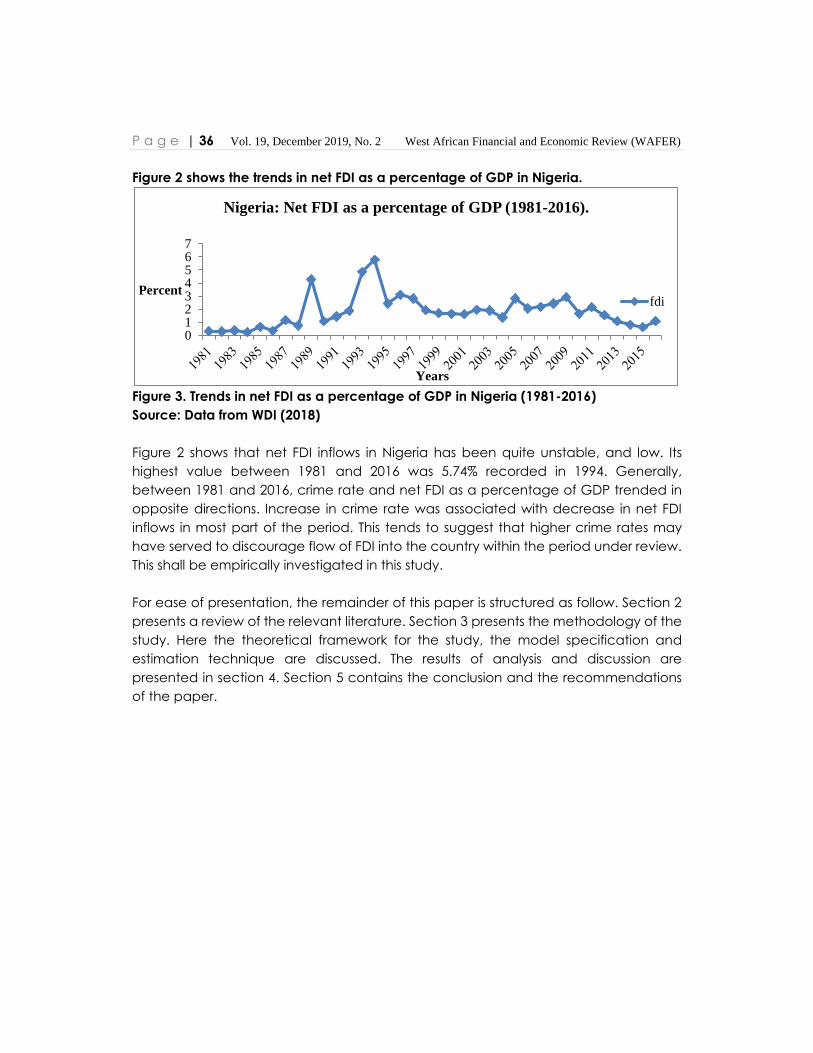
P a g e | 36 Vol. 19, December 2019, No. 2 West African Financial and Economic Review (WAFER)
Figure 2 shows the trends in net FDI as a percentage of GDP in Nigeria.
Figure 3. Trends in net FDI as a percentage of GDP in Nigeria (1981-2016)
Source: Data from WDI (2018)
Figure 2 shows that net FDI inflows in Nigeria has been quite unstable, and low. Its
highest value between 1981 and 2016 was 5.74% recorded in 1994. Generally,
between 1981 and 2016, crime rate and net FDI as a percentage of GDP trended in
opposite directions. Increase in crime rate was associated with decrease in net FDI
inflows in most part of the period. This tends to suggest that higher crime rates may
have served to discourage flow of FDI into the country within the period under review.
This shall be empirically investigated in this study.
For ease of presentation, the remainder of this paper is structured as follow. Section 2
presents a review of the relevant literature. Section 3 presents the methodology of the
study. Here the theoretical framework for the study, the model specification and
estimation technique are discussed. The results of analysis and discussion are
presented in section 4. Section 5 contains the conclusion and the recommendations
of the paper.
01234567
Percent
Years
Nigeria: Net FDI as a percentage of GDP (1981-2016).
fdi

Vol. 19, December 2019, No. 2 West African Financial and Economic Review (WAFER) P a g e | 37
2.0 Literature Review
2.1 Theoretical Literature
There exist numerous theories explaining the determinants of FDI. Each of the theories
identifies at least one factor explaining FDI inflows to an economy. Thus, Economists
are of the view that there is no generally accepted theory of determinants of FDI, and
that any model explaining the amount of FDI that flows into an economy must be
derived from a combination of several theories (Agarwal, 1980; Feath, 2009; Denisia,
2010).
Denisia (2010) classified the theories of FDI into four, namely: The production cycle
theory of Vernon; theory of exchange rates and imperfect capital markets; the
internalisation theory; and the eclectic paradigm of Dunning. The production cycle
theory was developed by Vernon in 1966. It was used to explain foreign investments
made by United States (U. S) corporations in Western Europe after the Second World
War. The theory identified four stages of production cycle namely: innovation, growth,
maturity and decline. The first stage involves creation of new innovative products by
U. S. corporations to serve the domestic markets and also to export surplus to Western
Europe where there was increased demand for products manufactured in the U. S. This
continues as the U. S. firms go through the growth and maturity stages since they had
technological advantage over international competitors. Overtime, Western Europe
firms began to copy and imitate the technologies of U. S. firms and to produce items
similar to those imported from the U. S. To maintain their market shares in local markets
of Europe, U. S. firms reacted by setting up plants in Western Europe. Thus the summary
of this theory is that the desire by multinationals (which are key channels through which
FDI is channeled into an economy) to maintain market shares of their products in
domestic market is a determinant of foreign direct investment in a host economy. A
drawback of this theory is that it ignored the fact that American multinational
corporations also made investment in countries for production of goods in which they
did not have any technological advantage during the period.
Proponents of the theory of exchange rate and imperfect capital markets argue that
multinational corporations (MNCs) move into and set up production facilities in
countries with weak or undervalued currencies, so as to sell their products to countries
whose currencies are strong or overvalued (Moosa, 2012). Thus, the theory predicts
positive effect of exchange rate devaluation or depreciation on FDI inflow.
P a g e | 38 Vol. 19, December 2019, No. 2 West African Financial and Economic Review (WAFER)
The internalisation theory is based on domestic transactions cost. It predicts that a firm
will decide to set up production plant(s) in foreign markets where costs of transactions
(exporting and licensing a product to another country) are quite high in home markets.
Thus, the firm internalises the transaction cost, and set up production plants/facilities in
another country (Blonigen, 1997). Hymer (1976) argues that firms undertake foreign
investment if the relative cost of operating abroad is less than the transaction cost.
The Eclectic paradigm, initially known as the Eclectic theory developed by Dunning
(1958, 2001) is an extension of the internalisation theory. It is also referred to as the OLI
(ownership, location and internalisation) model or framework for determination of
international production. The ownership or specific advantage refers to the
competitive advantage of the firm wishing to engage in foreign direct investment. The
greater the firm’s competitive advantage, the more likely it is to engage in foreign
production. On the location advantage, firms are attracted to, and tend to engage
in foreign production in locations where there is abundance of immobile natural or
created resources which they require to use jointly with their competitive or ownership
advantage. The internalisation advantage derives from the internalisation theory. As
firm is more likely to engage in foreign production if the advantage of internalising its
domestic transaction cost and engaging in foreign production exceeds the cost of
licensing its technology or product(s) in another country.
Several other theories exists which attribute firms’ decision for FDI or international
production to market size, trade openness, and other economic factor (Demiran &
Masca, 2008; Faeth, 2009). However, Hosseini (2005) attempted to explain the decision
by multinational firms to engage in FDI in other countries. According to Hosseini (2005,
p. 535) “culture (with indicators such as ethnicity, religion, etc.) is important for studying
the behavior of multinational enterprises, in their investment and other activities”.
Where the cultures of the home country of the MNCs differ significantly from that of
the targeted foreign market, this creates uncertainties which adversely affect the
decision for international production.
The Halo effect theory of FDI determination attributes firms’ decision to engage in
foreign direct investment in a country to investors’ broad impression of the country
based on the level of crime in specific locations across the country. Thus, this theory
identifies crime rate as a determinant of FDI inflow into a country.

Vol. 19, December 2019, No. 2 West African Financial and Economic Review (WAFER) P a g e | 39
2.2 Empirical Literature
Several studies have been conducted to examine the effect of crime on FDI inflows.
In this section, we review some of the empirical studies.
Ashby and Ramos (2013) investigated the effect of violent crime on FDI from 116
countries into different sectors of the 32 states of Mexico from 2004 to 2010. In the study,
number of reported murders was used to proxy regional organised crime, and Granger
causal analysis was employed for the analysis. The study found that organised crime
deters FDI inflows to financial services, commerce and agriculture sectors. However,
increased crime was found to be associated with increased FDI inflows in the oil and
gas sectors. Inflow of FDI to manufacturing sector was found to be unaffected by
violent crime. Similar study by Blanco, Ruiz, Sawyer and Wooster (2015) examined the
effect of crime on FDI inflows in different sectors (primary, secondary and tertiary) in
Latin American and Caribbean countries during the period from 1996 to 2010. Three
different crime-related variables namely homicide, crime victimization and an index
of organized crime were used for the study. The study found that higher crime
victimization and organised crime were associated with lower FDI inflows to the tertiary
sector. It found no robust evidence of significant effect of crime on FDI in the primary
and secondary sectors. The study recommended intensification of efforts by the
government to combat crime in the regions.
Daniele and Marani (2011) investigated the effect of organised crime on FDI inflows in
Italian provinces using panel data analysis. In the study, organised crime is measured
as the number of cases of reported crimes perpetrated by the mafia crime
organisation. The study found an inverse relationship between organised crime and
FDI. The result, according to the researchers, suggests that organised crime served as
deterrent to foreign investors as it renders the investment environment unfavourable
for FDI. A previous study by Daniele (2010) also concluded that high level of crime in
Southern Italy negatively affects economic outcomes, thereby creating notable
distortions in local markets and a business climate unfavourable to foreign and
domestic investment.
Helmy (2012) examined the effect of corruption, homicide and macroeconomic
factors on FDI flows to the Middle East and North Africa (MENA) region during the 2003-
2009, using different panel settings (fixed effects model estimated with the least
squares estimator, and a dynamic specification estimated using the system
generalised method of moments (GMM). The study found positive and significant
effect of corruption on FDI. It also found that homicides and tax adversely affected FDI
inflows into the region. Further evidences from the study are that macroeconomic

P a g e | 40 Vol. 19, December 2019, No. 2 West African Financial and Economic Review (WAFER)
factors such as per capita income, trade openness, freedom and security of
investment positively and significantly affected FDI inflows to the region. Thus there is
need to combat crime (in the form of homicide and corruption) to enhance the
attractiveness of the region to FDI.
The impact of crime on firm entry across municipal regions in South Africa during the
period from 2003 to 2011 was examined in the study by Mahofa, Sundaram and
Edwards (2016). Alternative estimations involving pooled OLS and fixed effect
controlled OLS were performed to achieve the study objective. The results indicated
that crime (contact crime, property crime, and household crime) negatively affected
entry of new firms into South Africa’s municipal regions.
Brown and Hibbert (2017) examined the effect of violent crime proxied by homicidal
rates on FDI inflows in a sample of 67 countries in the period from 1997 to 2012, using
OLS fixed effect and generalized method of moments (GMM) specifications. The study
found that violent crime discouraged inflows of FDI into the economies. The
researchers recommended that efforts should be made to address crimes so as to
stem their effect on growth-enhancing FDI.
Afriyanto (2017) investigated the effect of crime on FDI in a sample of 31 provinces of
Indonesia during the period from 2005 to 2015. The study found that crime negatively
affected inflow of FDI into the provinces. The study therefore recommended that in
addition to pursuing other policies to attract FDI, the government of Indonesia should
also pay attention to incidence of crime in each of the provinces.
Ramos and Ashby (2017) investigated the effect of violent crime (homicides) on FDI in
the states of Mexico in the period from 2001 to 2015. Fixed effect and system GMM
models were employed for the analysis. The study found an inverse relationship
between homicides and inward FDI, suggesting that high rate of violent crime
negatively affects inflow of FDI to the states. Cabral, Mollick and Saucedo (2018) also
studied the effect of violent crime on FDI inflows in the 32 subnational states of Mexico
using quarterly data that span the period from 2005 to 2015. The study found that
homicide and theft negatively and significantly affects FDI inflows to the country. The
effects of other crimes on FDI inflows were found to be statistically not significant. In
view of the observation that homicide and theft served as deterrence to inflow of FDI
in subnational states, there is therefore need for the government to take steps to curb
homicide and theft in the country, so as to enhance the attractiveness of various
subnational states to foreign investment.
Vol. 19, December 2019, No. 2 West African Financial and Economic Review (WAFER) P a g e | 41
In Nigeria, the Nigerian Communications Commission, NCC (2018) attempted to
examine the effect of cyber-crime on FDI inflows during the period from 2013 to 2016
using trend analysis to investigate the effect of cybercrime on FDI inflows to Nigeria
during the period from 2013 to 2016. The study found that cyber-attacks either deter
foreign investors from continuing their business or setting up new ones in the country.
The study only focuses on the relationship between cyber-crime and FDI inflows in
Nigeria, ignoring the other categories of crime. Moreover the study space is quite
narrow and the methodology applied is less sophisticated. This study improves on the
NCC’s study by considering the effect of crime in a broader sense of the number of
reported criminal cases (not just cyber-attacks) on FDI inflows over a wider scope of
1981 to 2016 using a more advanced econometric technique.
3.0 Methodology
3.1. Theoretical Framework and Model
The study follows the behavioural approach to modeling FDI decision developed by
Hosseini (2005). This approach highlights the superiority of behavioural economics
theory of FDI to other theories and identifies behavioural factors that are germane to
attracting FDI to an economy. In adopting this approach, we build on the Halo Effect
theory which attributes a country’s attractiveness to FDI to foreigner’s broad
impressions about the country based on crime rate (which is a behavioural factor)
therein (Ramos & Ashby, 2017). Thus FDI inflow to an economy may be regarded as a
function of crime rate.
The theoretical framework on determinants of FDI developed in Demirhan & Masca,
(2008) and Anyanwu (2011), identify market size (per capital income), inflation,
financial development, infrastructure, trade openness, government consumption
expenditure, etc. as determinants of FDI. Combining this with the position of the Halo
Effect theory, we derive our model to be estimated for the study as follow:
From the Halo Effect theory,
fdi = 𝑓(𝑐𝑟𝑖𝑚𝑒) (1)
From the theories on macroeconomic determinants of FDI,
fdi = 𝑓(𝑝𝑐𝑦, 𝑖𝑛𝑓, 𝑖𝑛𝑓𝑠𝑞, 𝑔𝑖, 𝑓𝑖𝑛𝑑𝑒𝑝, 𝑒𝑥𝑟𝑡, 𝑝𝑜𝑙𝑟𝑒𝑔) (2)
Agarwal (1980, p.740) noted that “there is not one, but a number of competing
theories with varying degrees of power to explain FDI”. Corroborating this, Feath (2009,
p.1) argues that “FDI should be explained more broadly by a combination of factors
P a g e | 42 Vol. 19, December 2019, No. 2 West African Financial and Economic Review (WAFER)
from a variety of theoretical models”. Our model to explain the determinants of FDI
inflows to Nigeria is therefore derived by combining equations (1) and (2) above as:
fdi = 𝑓(𝑐𝑟𝑖, 𝑝𝑐𝑦, 𝑖𝑛𝑓, 𝑖𝑛𝑓𝑠𝑞, 𝑔𝑖, 𝑓𝑖𝑛𝑑𝑒𝑝, 𝑒𝑥𝑟𝑡, 𝑝𝑜𝑙𝑟𝑒𝑔) (3)
Where fdi = foreign direct investment as a percentage of GDP, cr = crime rate,
measured as annual number of reported cases of crime per year (including homicides,
kidnapping, etc.) per 100, 000 of the population, pcy = per capita real GDP (proxy for
market size), inf = inflation rate, measured as annual percentage change in the
consumer price index, infsq (squared inflation) is incorporated to determine existence
or otherwise, of threshold effect of inflation, gi = globalistion index, which is a
composite index for economic, political and social-cultural integration or globalisation
computed by KOF Swiss Economic Institute, findep = index of financial depth, defined
by the World Bank (2018) as “private credit by deposit money banks and other
financial institutions to GDP”, and calculated by the Bank using the following deflation
method: {(0.5)*[Ft/P_et + Ft-1/P_et-1]}/[GDPt/P_at] where F is credit to the private
sector, P_e is end-of period CPI, and P_a is average annual CPI. Exrt = nominal (N/$)
exchange rate, Polreg = political regime (or regime type, using polity iv index whose
value range from -10 to +10, with -10 representing highly autocratic
regime/dictatorship, and +10 representing highly democratic regime).
The static (long-run) model is presented in its econometric form as:
𝑓𝑑𝑖𝑡 = β0 + β1𝑐𝑟𝑡 + β2 ln(𝑝𝑐𝑦𝑡) + β3𝑖𝑛𝑓𝑡 + β4𝑖𝑛𝑓𝑠𝑞𝑡 + β5𝑔𝑖𝑡 + β6𝑓𝑖𝑛𝑑𝑒𝑝𝑡 + β7 ln(𝑒𝑥𝑟𝑡)𝑡 +
β8𝑝𝑜𝑙𝑟𝑒𝑔𝑡 + ɛ𝑡 (4)
Equation 3 is the static specification of the econometric model.
The a priori expectations are: β1 < 0, β2 > 0, β3 > 0, β4 < 0, β5 > 0, β6 > 0, β7 > 0, β8 </> 0.
The autoregressive distributed lag (ARDL) modeling approach to cointegration and
error correction analysis developed by Pesaran, Shin and Smith (2001) was adopted to
analyse the relationship between the dependent variable and explanatory variables.
The choice of this approach was informed by its flexibility in application in that it can
be applied in cases of mixed order of integration of data, and the fact that it yields
consistent and efficient long-run coefficient estimates valid t-statistics even in the
presence of regressor endogeneity inherent among cointegrated regressors. The ARDL
model is specified as:
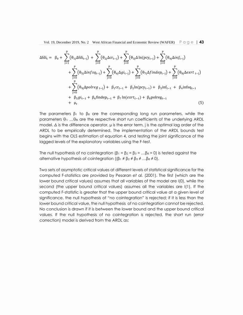
Vol. 19, December 2019, No. 2 West African Financial and Economic Review (WAFER) P a g e | 43
∆fdit = β0 + ∑(θ1j∆fdit−j)
p
j=1
+ ∑(θ2j∆crt−j)
p
j=0
+ ∑(θ3j∆ ln(pcyt−j)
p
j=0
+ ∑(θ4j∆𝑖𝑛𝑓t−j)
P
j=0
+ ∑(θ5j∆𝑖𝑛𝑓𝑠𝑞t−j)
P
j=0
+ ∑(θ6j∆𝑔𝑖t−j)
P
j=0
+ ∑(θ7j∆𝑓𝑖𝑛𝑑𝑒𝑝t−j)
p
j=0
+ ∑(θ8j∆𝑒𝑥𝑟𝑡 t−j)
p
j=0
+ ∑(θ9j∆𝑝𝑜𝑙𝑟𝑒𝑔 t−j) + β1crt−1 + β2ln (pcyt−1) + β3inft−1 + β4infsqt−1
p
j=0
+ β5𝑔𝑖t−1 + β6findept−1 + β7 ln(𝑒𝑥𝑟𝑡𝑡−1) + β8polregt−1
+ μ𝑡 (5)
The parameters β1 to β8 are the corresponding long run parameters, while the
parameters θ1i …θ8i are the respective short run coefficients of the underlying ARDL
model. Δ is the difference operator, µ is the error term, j is the optimal lag order of the
ARDL to be empirically determined. The implementation of the ARDL bounds test
begins with the OLS estimation of equation 4, and testing the joint significance of the
lagged levels of the explanatory variables using the F-test.
The null hypothesis of no cointegration (β1 = β2 = β3 = …β8 = 0) is tested against the
alternative hypothesis of cointegration ((β1 ≠ β2 ≠ β3 ≠ …β8 ≠ 0).
Two sets of asymptotic critical values at different levels of statistical significance for the
computed F-statistics are provided by Pesaran et al. (2001). The first (which are the
lower bound critical values) assumes that all variables of the model are I(0), while the
second (the upper bound critical values) assumes all the variables are I(1). If the
computed F-statistic is greater that the upper bound critical value at a given level of
significance, the null hypothesis of “no cointegration” is rejected; if it is less than the
lower bound critical value, the null hypothesis of no cointegration cannot be rejected.
No conclusion is drawn if it is between the lower bound and the upper bound critical
values. If the null hypothesis of no cointegration is rejected, the short run (error
correction) model is derived from the ARDL as:
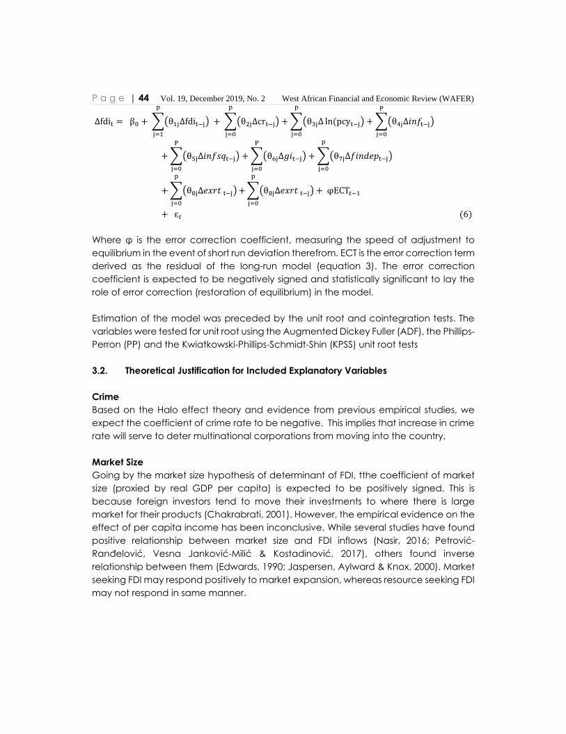
P a g e | 44 Vol. 19, December 2019, No. 2 West African Financial and Economic Review (WAFER)
∆fdit = β0 + ∑(θ1j∆fdit−j)
p
j=1
+ ∑(θ2j∆crt−j)
p
j=0
+ ∑(θ3j∆ ln(pcyt−j)
p
j=0
+ ∑(θ4j∆𝑖𝑛𝑓t−j)
P
j=0
+ ∑(θ5j∆𝑖𝑛𝑓𝑠𝑞t−j)
P
j=0
+ ∑(θ6j∆𝑔𝑖t−j)
P
j=0
+ ∑(θ7j∆𝑓𝑖𝑛𝑑𝑒𝑝t−j)
p
j=0
+ ∑(θ8j∆𝑒𝑥𝑟𝑡 t−j)
p
j=0
+ ∑(θ8j∆𝑒𝑥𝑟𝑡 t−j)
p
j=0
+ φECT𝑡−1
+ ɛ𝑡 (6)
Where φ is the error correction coefficient, measuring the speed of adjustment to
equilibrium in the event of short run deviation therefrom. ECT is the error correction term
derived as the residual of the long-run model (equation 3). The error correction
coefficient is expected to be negatively signed and statistically significant to lay the
role of error correction (restoration of equilibrium) in the model.
Estimation of the model was preceded by the unit root and cointegration tests. The
variables were tested for unit root using the Augmented Dickey Fuller (ADF), the Phillips-
Perron (PP) and the Kwiatkowski-Phillips-Schmidt-Shin (KPSS) unit root tests
3.2. Theoretical Justification for Included Explanatory Variables
Crime
Based on the Halo effect theory and evidence from previous empirical studies, we
expect the coefficient of crime rate to be negative. This implies that increase in crime
rate will serve to deter multinational corporations from moving into the country.
Market Size
Going by the market size hypothesis of determinant of FDI, tthe coefficient of market
size (proxied by real GDP per capita) is expected to be positively signed. This is
because foreign investors tend to move their investments to where there is large
market for their products (Chakrabrati, 2001). However, the empirical evidence on the
effect of per capita income has been inconclusive. While several studies have found
positive relationship between market size and FDI inflows (Nasir, 2016; Petrović-
Ranđelović, Vesna Janković-Milić & Kostadinović, 2017), others found inverse
relationship between them (Edwards, 1990; Jaspersen, Aylward & Knox, 2000). Market
seeking FDI may respond positively to market expansion, whereas resource seeking FDI
may not respond in same manner.
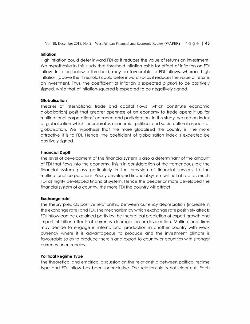
Vol. 19, December 2019, No. 2 West African Financial and Economic Review (WAFER) P a g e | 45
Inflation
High inflation could deter inward FDI as it reduces the value of returns on investment.
We hypothesise in this study that threshold inflation exists for effect of inflation on FDI
inflow. Inflation below a threshold, may be favourable to FDI inflows, whereas high
inflation (above the threshold) could deter inward FDI as it reduces the value of returns
on investment. Thus, the coefficient of inflation is expected a priori to be positively
signed, while that of inflation-squared is expected to be negatively signed.
Globalisation
Theories of international trade and capital flows (which constitute economic
globalisation) posit that greater openness of an economy to trade opens it up for
multinational corporations’ entrance and participation. In this study, we use an index
of globalisation which incorporates economic, political and socio-cultural aspects of
globalisation. We hypothesis that the more globalised the country is, the more
attractive it is to FDI. Hence, the coefficient of globalisation index is expected be
positively signed.
Financial Depth
The level of development of the financial system is also a determinant of the amount
of FDI that flows into the economy. This is in consideration of the tremendous role the
financial system plays particularly in the provision of financial services to the
multinational corporations. Poorly developed financial system will not attract as much
FDI as highly developed financial system. Hence the deeper or more developed the
financial system of a country, the more FDI the country will attract.
Exchange rate
The theory predicts positive relationship between currency depreciation (increase in
the exchange rate) and FDI. The mechanism by which exchange rate positively affects
FDI inflow can be explained partly by the theoretical prediction of export-growth and
import-inhibition effects of currency depreciation or devaluation. Multinational firms
may decide to engage in international production in another country with weak
currency where it is advantageous to produce and the investment climate is
favourable so as to produce therein and export to country or countries with stronger
currency or currencies.
Political Regime Type
The theoretical and empirical discussion on the relationship between political regime
type and FDI inflow has been inconclusive. The relationship is not clear-cut. Each

P a g e | 46 Vol. 19, December 2019, No. 2 West African Financial and Economic Review (WAFER)
regime type (autocracy or democracy) may attract different type of FDI depending
on the policy the government is implementing. Where the policies implemented are
attractive to FDI, it is expected that more FDI will flow into the country irrespective of
whether they are implemented by autocratic or democratic government. Jensen
(cited in Konki and Notermans, 2017) argues that transparency which is characteristic
of democracy is favourable to investment. O’Donnell’s theory argued that foreign
companies are attracted to authoritarian regime as it offers the opportunity of
monopolistic position and financial incentives in the host countries with the possibility
of higher returns on investment than in democracies (Konki and Notermans, 2017).
Thus, the coefficient of political regime variable could be expected either positively or
negatively signed. It is therefore indeterminate.
3.3. Data
Data used for the estimation are annual time series data spanning the period from
1981 to 2016. They were sourced from the World Bank’s World Development Indicators
of 2018, the World Banks’s Global Financial Development Database, 2018, the
Nigeria’s National Bureau of Statistics Statistical Bulletin (2018) and the KOF Swiss
Economic Institute Globalisation Index, 2018.
4.0 Results and Discussions
4.1 Unit Root and Cointegration Tests
The results of the unit root test for the variables are presented in Table 1.
Table 1. Unit Root Test Results.
Augmented Dickey Fuller (ADF) Unit Root Test
Level First Difference I(d)
Variables ADF
test
stat.
Critical
Value
(5%)
Inference ADF test
stat.
Critical
Value
(5%)
Inference
Fdi -3.24 -3.54 NS -8.13 -3.55 S 1
Crime -1.99 -3.54 NS -5.59 -3.55 S 1
ln(pcy) -1.47 -3.55 NS -3.56 -3.55 S 1
Inf -3.84 -3.55 S - - - 0
GI -2.40 -3.54 NS -5.80 -3.55 S 1
Findep -2.37 -3.55 NS -3.90 -3.55 S 1
Log(exrt) -1.24 -3.54 NS -5.36 -3.55 S 1
Polreg -3.89 -3.55 S - - - 0

Vol. 19, December 2019, No. 2 West African Financial and Economic Review (WAFER) P a g e | 47
Phillips-Perron (PP) Unit Root Test
Level First Difference I(d)
Variables PP test
stat.
Critical
Value
(5%)
Inference PP test
stat.
Critical
Value
(5%)
Inference
Fdi -3.17 -3.54 NS -21.58 -3.55 S 1
Cr -1.91 -3.54 NS -5.70 -3.55 S 1
ln(pcy) -3.08 -3.54 NS -3.56 -3.55 S 1
Inf -2.73 -3.54 NS -9.62 -3.55 S 1
GI -2.53 -3.54 NS -5.81 -3.55 S 1
Findep -1.64 -3.54 NS -4.09 -3.55 S 1
Log(exrt) -1.27 -3.54 NS -5.63 3.55 S 1
Polreg -3.02 -3.54 NS -5.41 -3.55 S 1
Findep -1.64 -3.54 NS -4.09 -3.55 S 1
Kwiatkowski-Phillips-Schmidt-Shin (KPSS) Unit Root Test
Level First Difference I(d)
Variables KPSS
test
stat.
Critical
Value
(5%)
Inference KPSS test
stat.
Critical
Value
(5%)
Inference
Fdi 0.17 0.46 S - - - 0
Cr 0.16 0.15 NS 0.09 0.15 S 1
ln(pcy) 0.20 0.15 NS 0.12 0.15 S 1
Inf 0.11 0.15 S - - - 0
GI 0.10 0.15 S - - - 0
Findep 0.17 0.15 NS 0.07 0.15 S 1
Log(exrt) 0.20 0.15 NS 0.08 0.15 S 1
Polreg 0.43 0.46 S - - - 0
NS = Non-stationary; S = Stationary; I(d) = Order of integration
Whereas the result of PP test for unit root indicates that the variables are stationary at
first differences, the ADF and the KPSS test results indicate that the variables are of
mixed order of integration. The orders of integration of the variables of a model to be
estimated determine the approach to testing for cointegration relationships among
the variables and also in many cases, the estimation technique to be adopted for
estimation of the model. In this study, the ARDL bounds testing approach to
cointegration and error correction analysis was employed because of its applicability,
irrespective of the order of integration of the variables, so long as none of them is I(2)

P a g e | 48 Vol. 19, December 2019, No. 2 West African Financial and Economic Review (WAFER)
(that is none is integrated of order 2). The result of the cointegration test is presented
in Table 2.
Table 2. ARDL Bounds Test
Sample: 1982-2016
Included Observation: 35
Null Hypothesis: No long-run relationships exists
Test Statistic Value K
F-statistic 18.20 8
Critical Value Bounds
Significance Lower (I0) Bound Upper (I1) Bound
10% 1.95 3.06
5% 2.22 3.39
2.5% 2.48 3.70
1% 2.79 4.10
The Bounds test for cointegration clearly rejects the null hypothesis that “No long-run
relationships exist” among the variables, as the F-statistic value of 18.20 is greater than
the upper bounds critical value even at the 1% significance level. Thus it can be
inferred that the variables are cointegrated.
4.2 Model Estimation
The result of estimation of the short-run and long-run models based on the estimated
ARDL (1,1,1,1,1,1,1,1) model (shown in Table A1 in the Appendix) is presented in Table
3.
Table 3. Model Estimation Result
Dependent Variable: fdi
Selected Model: ARDL (1,1,1,1,1,1,1,1,1)
Sample: 1981-2016
Included Observations: 35
Variable Coefficient T-stat Prob.
d(Crime) -0.02 -0.79 0.44
D(ln(pcy)) -11.51 -3.84 0.00
d(inf) 0.06 1.90 0.07
d(infsq) -0.00 -1.94 0.07
d(gi) 0.20 2.75 0.01
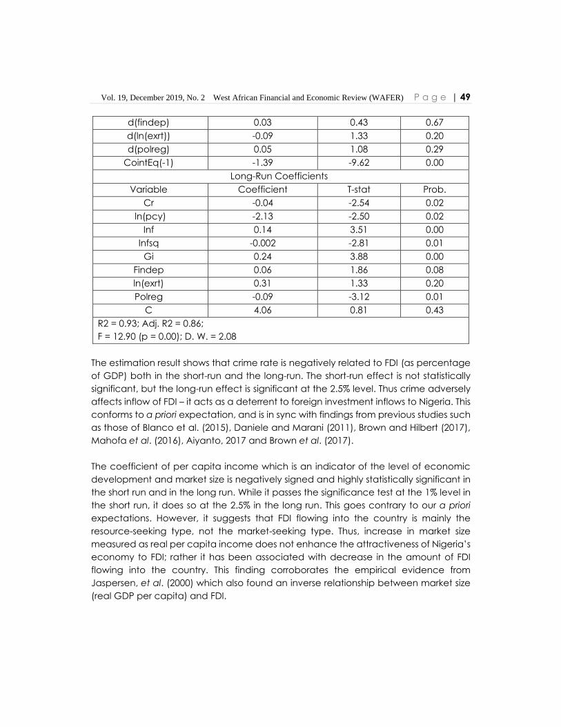
Vol. 19, December 2019, No. 2 West African Financial and Economic Review (WAFER) P a g e | 49
d(findep) 0.03 0.43 0.67
d(ln(exrt)) -0.09 1.33 0.20
d(polreg) 0.05 1.08 0.29
CointEq(-1) -1.39 -9.62 0.00
Long-Run Coefficients
Variable Coefficient T-stat Prob.
Cr -0.04 -2.54 0.02
ln(pcy) -2.13 -2.50 0.02
Inf 0.14 3.51 0.00
Infsq -0.002 -2.81 0.01
Gi 0.24 3.88 0.00
Findep 0.06 1.86 0.08
ln(exrt) 0.31 1.33 0.20
Polreg -0.09 -3.12 0.01
C 4.06 0.81 0.43
R2 = 0.93; Adj. R2 = 0.86;
F = 12.90 (p = 0.00); D. W. = 2.08
The estimation result shows that crime rate is negatively related to FDI (as percentage
of GDP) both in the short-run and the long-run. The short-run effect is not statistically
significant, but the long-run effect is significant at the 2.5% level. Thus crime adversely
affects inflow of FDI – it acts as a deterrent to foreign investment inflows to Nigeria. This
conforms to a priori expectation, and is in sync with findings from previous studies such
as those of Blanco et al. (2015), Daniele and Marani (2011), Brown and Hilbert (2017),
Mahofa et al. (2016), Aiyanto, 2017 and Brown et al. (2017).
The coefficient of per capita income which is an indicator of the level of economic
development and market size is negatively signed and highly statistically significant in
the short run and in the long run. While it passes the significance test at the 1% level in
the short run, it does so at the 2.5% in the long run. This goes contrary to our a priori
expectations. However, it suggests that FDI flowing into the country is mainly the
resource-seeking type, not the market-seeking type. Thus, increase in market size
measured as real per capita income does not enhance the attractiveness of Nigeria’s
economy to FDI; rather it has been associated with decrease in the amount of FDI
flowing into the country. This finding corroborates the empirical evidence from
Jaspersen, et al. (2000) which also found an inverse relationship between market size
(real GDP per capita) and FDI.
P a g e | 50 Vol. 19, December 2019, No. 2 West African Financial and Economic Review (WAFER)
The effects of inflation and squared inflation are respectively positive and negative in
the short-run and in the long-run. These conform to a priori expectation. The effects are
significant at the 10% level in the short-run, and at 1% level in the long-run. This suggests
existence of threshold level of inflation. Below the threshold, inflation could be
favourable to growth. However, above the threshold, inflation could act as a deterrent
to FDI inflow. This observation is in sync with Obiamaka, Onwumere and Okpa (2011)
and Tsaurai (2018).
The depth of the financial system is found to be a significant determinant of FDI inflows
in Nigeria. The effect of financial depth on FDI inflows in Nigeria is positive, and
significant at the 2.5% significance level. This suggests that financial system
development enhances the attractiveness of the country to inward FDI. The result is
consistent with the empirical evidence from Desbordes and Wei (2014), Varnamkhasti
and Mehregan (2014), Kiiza and Seguya (2015), Shah (2017) and Dellis (2018).
The short-run and the long-run effects of globalisation on FDI inflows in Nigeria are
observed to be positive and significant at the 1% level. These conform to a priori
expectations. The findings suggests that highly globalized economies tend to be
attractive to FDI inflow. The more integrated the country (Nigeria) is with the rest of the
world, the more FDI it attracts. This is in line with evidence from previous studies such as
those of Kandiero and Chitiga (2006), Dima (2016) and Brun and Gnangnon (2017),
and it suggests that (cautious) removal of barriers to free flow of cross-border trade will
engender increase in inflow of FDI to Nigeria’s economy.
The short-run and the long-run effects of exchange rate on FDI inflow in Nigeria are
respectively positive and negative, but none is statistically significant. These suggest
that the exchange rate of the Naira plays no significant role in the determination of
the amount of FDI that flows into the country.
The short-run, effect of political regime on FDI inflow is positive, as expected, but not
statistically significant. However, its long-run effect is negative and significant at the 1%
level. This suggests that autocratic government tends to favour FDI inflows. This
validates the O’Connell’s theory of FDI. It suggests that foreign investors engaging in
FDI in Nigeria’s economy may have preferred to channel their investments in more
autocratic government. It also suggests that FDI inflow is not a matter of polity but a
matter of policy as observed by Konki & Notermans (2017). This is in view of the fact,
that democratic government could also be autocratic in dispensation. Policies
favouring FDI inflows may have been implemented by governments that were more
autocratic in their operations. Caution should however be exercised in recommending
Vol. 19, December 2019, No. 2 West African Financial and Economic Review (WAFER) P a g e | 51
policy based on the observed negative coefficient of political regime variable as it
does not necessarily imply that the government has to be more autocratic to attract
FDI.
The coefficient of the lagged error correction term (CointEq) is, as expected,
negatively signed and statistically significant at the 1%. This further confirms the
existence of long run relationship between the explanatory variables and the
dependent variable. The coefficient value of -1.39 implies that the error correction
process (that is the convergence toward equilibrium in the relationship in the event of
short-run deviation therefrom) is oscillatory instead of being monotonic or asymptotic
(Narayan and Smith, 2005).
The coefficient of determination of the model is quite impressive, as it indicates that
the model has a high goodness of fit or explanatory power. The model explains about
93% of the systematic variation in the dependent variable. The reliability of the
explanatory power is indicated by the F-statistic of 12.90 which easily passes the
significance test at the 1% level, indicating the joint significance of the explanatory
variables. The Durbin-Watson (D. W.) of 2.08 indicates absence of problem of
autocorrelation in the model. The test for normality of the residual shows that the
residuals are normally distributed as indicated by the probability of the Jarque-Bera
statistic (p = 0.54) which fails to reject the hypothesis of normality. This is shown in the
Appendix of this paper. The Ramsey RESET test result also shown in the Appendix reveals
that the functional form of the ARDL model is correctly specified. The model could
therefore be reliably deployed for policy formulation.
5.0 Concluding Remarks and Recommendations
Crime serves as a deterrent to participation by multinational corporations in Nigeria.
There is therefore the need to intensify efforts to holistically combat crime in the country
in order to attract more FDI to complement domestic capital so as to enhance the
growth of the nation’ economy. The government of Nigeria should strengthen the
nation’s anti-crime agencies and the legal and criminal justice systems to holistically
combat crime in the country. Greater but cautious integration of the country’s trade,
finance, politics and culture with the rest of the world will enhance the attractiveness
of the country to FDI. There is need for the monetary authority to strive to achieve levels
of inflation not detrimental to FDI inflows, and develop the financial system as these
will also enhance the attractiveness of the nation’s economy to FDI.

P a g e | 52 Vol. 19, December 2019, No. 2 West African Financial and Economic Review (WAFER)
References
Afriyanto, M. M. (2017). The Impact of Crime on Foreign Direct Investment.
Economic Journal of Emerging Markets, 9(2), October, 189-198.
Agarwal, J. P. (1980). Determinants of Foreign Direct Investment: A Survey.
Weltwirtschaftliches Archiv, 116(4), 739-773.
Akinlo, A. E. (2017). Determinants of Foreign Direct Investment in Nigeria: A Markov
Regime-Switching Approach. Review of Innovation and Competitiveness, 3(1),
21-48.
Anyanwu, J. C. (2011). Determinants of Foreign Direct Investment Inflows to Africa,
1980-2007.
African Development Bank Group Working Paper Series, No. 136, September.
Arawomo, O. & Apanisile, J. F. (2018). Determinants of Foreign Direct Investment in the
Nigerian Telecommunication Sector. Modern Economy, 9, 907-923.
Asogwa, F. O. & Osondun, M. C. (2014). The Impact of Foreign Direct Investment on
Economic Growth in Nigeria. IOSR Journal of Economics and Finance, 3(5),
May-June, 37-45.
Ashby, N. J. & Ramos, M. A. (2013). Foreign Direct Investment and Industry Response to
Organised Crime: The Mexican Case. European Journal of Political Economy,
30, June, 880-91.
Blanco, L., Ruiz, I., Sawyer, W. C. & Wooster, R. (2015). Crime, Institutions and Sector-
Specific FDI in Latin America. Portland State University Economics Faculty Publications
and Presentations. Paper 47.
Blonigen, B. A. (1997). Firm-Specific Assets and the Link between Exchange Rates and
Foreign Direct Investment. The American Economic Journal, 87(3), 447-465.
Brown, L. & Hibbert, K. (2017). The Effect of Crime on Foreign Direct Investment: A Multi-
Country Panel Data Analysis. The Journal of Developing Areas, 51(1), 295-307.
Brun, J. & Gnangnon, S. K. (2017). Does Trade Openness contribute to driving Financing
Flows for Development? WTO Working Paper ERSD-2017-06, March.
Buonanno, P. (2003). The Socioeconomic Determinants of Crime. A Review of the
Literature. Working Papers 63, University of Milano-Bicocca, Department of
Economics, revised Nov 2003.
Cabral, Mollick and Saucedo (2018). Foreign Direct Investment in Mexico, Crime, and
Economic Forces. Contemporary Economic Policy, 37(1), January, 68-85.
Carbonell, J. B. & Werner, R. A. (2018). Does Foreign Direct Investment Generate
Economic Growth? A New Empirical Approach Applied to Spain. Economic
Geography, 94(4), 425-456.
Vol. 19, December 2019, No. 2 West African Financial and Economic Review (WAFER) P a g e | 53
Charkrabarti, A. (2001). The Determinants of Foreign Direct Investment: Sensitivity
Analyses of Cross-Country Regressions. Kyklos, 54(1), 89-114.
Daniele, V. (2010). The Burden of Crime on Development and FDI in Southern Italy.
Italian Journal of International Affairs, 45(2), 103-117.
Daniele, V. & Marani, U. (2011). Organized Crime, The Quality of Local Institutions and
FDI in Italy: A Panel Data Analysis. European Journal of Political Economy, 27(1),
March, 132-142.
Demiran E. & Masca, M. (2008). Determinants of Foreign Direct Investment Flows to
Developing Countries: A Cross-Sectional Analysis. Prague Economic Papers, 4, 356-
2008.
Denisia, V. (2010). Foreign Direct Investment Theories. European Journal of
Interdisciplinary
Studies, 3, December, 53-59.
Dellis, K. (2018). Financial Development and FDI Flows: Evidence from Advanced
Economies.
Bank of Greece Eurosystem Working Paper 254, December.
Demirhan, E. & Masca, M. (2008). Determinants of Foreign Direct Investment Flows to
Developing Countries: A Cross-Sectional Analysis. Prague Economic Papers, 4,
356-369.
Desbordes, R. & Wei, S. (2014). The Effects of Financial Development on Foreign Direct
Investment. Policy Research Working Paper No. 7065. World Bank Group,
Washington, DC.
Dima S. (2016). Globalisation, Trade Openness and Foreign Direct Investment in
Romania. Studia Universitatis “Vasile Goldis” Arad – Economics Series, 26(4), 41-
53.
Dunning, J. H. (2001). The Eclectic (OLI) Paradigm of International Production: Past,
Present and Future. International Journal of the Economics of Business, 8(2), 173-
190.
Dunning, J.H. (1958). American Investment in British Manufacturing Industry, London:
Allen & Unwin.
Edwards, S. (1990). Capital Flows, Foreign Direct Investment, and Dept - Equity Swaps
in Developing Countries. NBER Working Paper No. 3497.
Faeth, I. (2009). Determinants of Foreign Direct Investment – A Tale of Nine Theoretical
Models. Journal of Economic Surveys, 23(1), 165-196.
Guerin, S. S. & Manzocchi, S. (2009). Political Regime and FDI from Advanced to
Emerging Countries. Review of World Economics, 145(1), April, 75-91.
Helmy, H. E. (2012). The Impact of Corruption on FDI: Is MENA an Exception?
International Review of Applied Economics, 27(4), 491-514.

P a g e | 54 Vol. 19, December 2019, No. 2 West African Financial and Economic Review (WAFER)
Hosseni, H. (2005). An Economic Theory of FDI: A Behavioral Economics and Historicall
Approach. The Journal of Social Economics, 34, 528-541.
Hymer, S. 1976 (1960). The International Operations of Nation Firms: A Study of Foreign
Direct Investment, Cambridge: MIT Press.
Iamsiraroj, S. & Ulubasoglu, M. A. (2015). Foreign Direct Investment and Economic
Growth: A Relationship or Wishful Thinking? Economic Modelling, 51,
December, 200-213.
Igbinedion, S. O & Ebomoyi, I. (2017). Socio-Economic Determinants of Crime: Further
Evidence From Nigeria. Annals of the University of Petroşani, Economics, 17(1),
2017, 101-114.
İmrohoroğlu, A., Merlo, M. & Rupert, P. (2006). Understanding the Determinants of
Crime. Federal Reserve Bank of Cleveland Working Paper 06-02.
Jaspersen, F. Z., Aylward, A. H. & Knox, A. D. (2000). The Effects of Risk on Private
Investment: Africa Compared with Other Developing Areas, in P. P. Collier, C. (Ed.),
Investment and Risk in Africa, New York: St Martin’s Press.
Kandiero, T. & Chitiga, M. (2006). Trade Openness and Foreign Direct Investment in
Africa. South African Journal of Economics and Management Sciences, 9(3),
355-370.
Khan, N., Ahmed, J., Nawaz, M., & Zaman, K. (2015). The Socio-Economic Determinants
of Crime in Pakistan: New Evidence on an Old Debate. Arab Economic and
Business Journal, 10(2), 73-81.
Kiiza, B. & Seguya, E. (2015). FDI and Economic Growth in the East African Community
Trade Bloc: Panel Co-integration Evidence. Review of Economics and Finance,
6(3), 88-101.
Konki, A. N. & Notermann, T. (2017). The Relationship between Political Regimes And
Foreign Direct Investment. Working Paper, School Of Business And Governance, Tallinn
University Of Technology.
Mahofa, G., Sundaram, A. & Edwards, L. (2016). Impact of Crime on Firm Entry:
Evidence from South Africa. Economic Research South Africa (ERSA) Working
Paper 652.
McGuire, J. (2004). Understanding Psychology and Crime: Perspectives on Theory and
Action, Berkshire: Open University Press.
Meera, A. K. & Jayakumar, M. D. (2006). Determinants of Crime in a Developing
Country: A Regression Model. Applied Economics, 27(5), 455-460.
Moosa, I. M. (2002). Foreign Direct Investment: Theory, Evidence and Practice, New
York, NY: Palgrave
Mottaleb, K. A. & Kalirajan, K. (2010). Determinants of Foreign Direct Investment in
Developing Countries: A Comparative Analysis. ASARC Working Paper 2010/13.

Vol. 19, December 2019, No. 2 West African Financial and Economic Review (WAFER) P a g e | 55
Narayan, P. K.& Smyth, R. (2005). What Determines Migration Flows from Low-Income
to High-Income Countries? An Empirical Investigation of Fiji–U.S. Migration 1972–
2001. Contemporary Economic Policy, 24(2), April, 332–342
Nasir, A. (2016). Market Size, Exchange Rate and Trade as a Determinant of FDI the
Case of Malaysia. American Journal of Business and Society, 1(4), 227-232.
NCC (2017). Final Report on: Effect of Cyber Crime on Foreign Direct Investment and
National Development, Abuja: Nigerian Communications Commission.
Obiamaka, P.E., Onwumere, J.U. & Okpara, G.C. (2011). Foreign Direct Investment and
Economic Growth in Nigeria: A Granger Causality Analysis. International
Journal of Current Research, 3(11), 225-232.
Offiong, A. I. & Atsu, I. A. (2014). Determinants of Foreign Direct Investment in Nigeria
(1980 - 2011). International Review of Management and Business Research,
3(3), September, 1538-1550.
Pesaran, M. H., Shin, Y. & Smith, R. (2001). Bounds Testing Approaches to the Analysis of
Level Relationships. Journal of Applied Econometrics, 16, 289-326.
Petrović-Ranđelović, M., Janković-Milić, V. and Kostadinović, I. (2017). Market Size as
a Determinant of the Foreign Direct Investment Inflows in the Western Balkans
Countries. Economics and Organization, 14(2), 93 – 104.
Ramos, M. A. & Ashby, N. J. (2017). The Halo Effect: Violent Crime and Foreign Direct
Investment. Multinational Business Review, 25(4), 287-306.
Shah, M. M. (2017). Financial Development and Foreign Direct Investment: The case of
Middle East and North African (MENA) Developing Nations. MPRA Paper No.
82013, October.
Swiss Economic Institute (2018). KOF Globalisation Index Database, Zurich: Swiss
Economic Institute.
Tsaurai, K. (2018). Investigating the Impact of Inflation on Foreign Direct Investment in
Southern Africa. ŒCONOMICA, 14(4), 597-611.
Varnamkhasti, J. G. & Mehregan, N. (2014). Financial Development as a Key
Determinant of FDI Inflow to Developing Countries. International Journal of
Humanities, 21(3), 17-43.
Wafure, O. G. & Nurudeen, A. (2010). Determinants of Foreign Direct Investment in
Nigeria: An Empirical Analysis. Global Journal of Human Social Science, 10(1),
April, 26-34.
World Bank (2018). Global Financial Development Report 2017 / 2018: Bankers without
Borders. Washington DC: The World Bank.

P a g e | 56 Vol. 19, December 2019, No. 2 West African Financial and Economic Review (WAFER)
APPENDIX
TABLE A1. ARDL MODEL
Dependent Variable: FDI
Method: ARDL
Date: 05/11/19 Time: 22:16
Sample (adjusted): 1982 2016
Included observations: 35 after adjustments
Maximum dependent lags: 1 (Automatic selection)
Model selection method: Akaike info criterion (AIC)
Dynamic regressors (1 lag, automatic): CR LOG(RGDPPC) INF INFSQ GI
FINDEP LOG(EXRT) POLREG
Fixed regressors: C
Number of models evalulated: 256
Selected Model: ARDL(1, 1, 1, 1, 1, 1, 1, 1, 1)
Variable Coefficient Std. Error t-Statistic Prob.*
FDI(-1) -0.391129 0.144552 -2.705811 0.0150
CR -0.019908 0.025104 -0.793022 0.4387
CR(-1) -0.039702 0.029444 -1.348416 0.1952
LOG(RGDPPC) -11.51024 2.999274 -3.837675 0.0013
LOG(RGDPPC(-1)) 8.540642 2.880252 2.965241 0.0087
INF 0.059948 0.031500 1.903141 0.0741
INF(-1) 0.139388 0.028012 4.976048 0.0001
INFSQ -0.000913 0.000472 -1.936072 0.0697
INFSQ(-1) -0.001395 0.000384 -3.636048 0.0020
GI 0.196144 0.071673 2.736652 0.0141
GI(-1) 0.141383 0.087713 1.611881 0.1254
FINDEP 0.026397 0.061061 0.432310 0.6710
FINDEP(-1) 0.055274 0.053171 1.039537 0.3131
LOG(EXRT) -0.093158 0.398542 -0.233748 0.8180
LOG(EXRT(-1)) 0.527905 0.421834 1.251451 0.2277
POLREG 0.045484 0.042267 1.076119 0.2969
POLREG(-1) -0.172107 0.051535 -3.339602 0.0039
C 5.645007 6.989244 0.807671 0.4304
R-squared 0.929348 Mean dependent var 1.861062
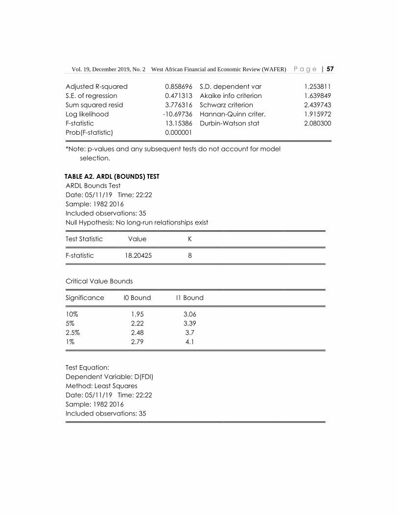
Vol. 19, December 2019, No. 2 West African Financial and Economic Review (WAFER) P a g e | 57
Adjusted R-squared 0.858696 S.D. dependent var 1.253811
S.E. of regression 0.471313 Akaike info criterion 1.639849
Sum squared resid 3.776316 Schwarz criterion 2.439743
Log likelihood -10.69736 Hannan-Quinn criter. 1.915972
F-statistic 13.15386 Durbin-Watson stat 2.080300
Prob(F-statistic) 0.000001
*Note: p-values and any subsequent tests do not account for model
selection.
TABLE A2. ARDL (BOUNDS) TEST
ARDL Bounds Test
Date: 05/11/19 Time: 22:22
Sample: 1982 2016
Included observations: 35
Null Hypothesis: No long-run relationships exist
Test Statistic Value K
F-statistic 18.20425 8
Critical Value Bounds
Significance I0 Bound I1 Bound
10% 1.95 3.06
5% 2.22 3.39
2.5% 2.48 3.7
1% 2.79 4.1
Test Equation:
Dependent Variable: D(FDI)
Method: Least Squares
Date: 05/11/19 Time: 22:22
Sample: 1982 2016
Included observations: 35
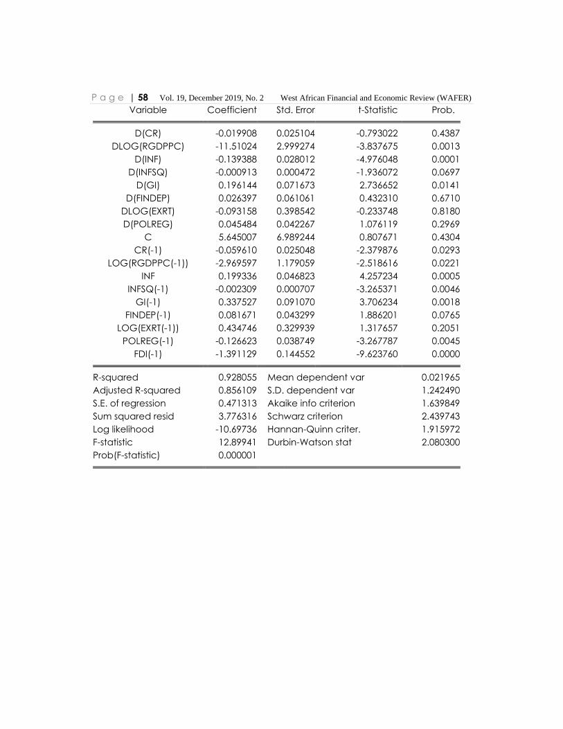
P a g e | 58 Vol. 19, December 2019, No. 2 West African Financial and Economic Review (WAFER)
Variable Coefficient Std. Error t-Statistic Prob.
D(CR) -0.019908 0.025104 -0.793022 0.4387
DLOG(RGDPPC) -11.51024 2.999274 -3.837675 0.0013
D(INF) -0.139388 0.028012 -4.976048 0.0001
D(INFSQ) -0.000913 0.000472 -1.936072 0.0697
D(GI) 0.196144 0.071673 2.736652 0.0141
D(FINDEP) 0.026397 0.061061 0.432310 0.6710
DLOG(EXRT) -0.093158 0.398542 -0.233748 0.8180
D(POLREG) 0.045484 0.042267 1.076119 0.2969
C 5.645007 6.989244 0.807671 0.4304
CR(-1) -0.059610 0.025048 -2.379876 0.0293
LOG(RGDPPC(-1)) -2.969597 1.179059 -2.518616 0.0221
INF 0.199336 0.046823 4.257234 0.0005
INFSQ(-1) -0.002309 0.000707 -3.265371 0.0046
GI(-1) 0.337527 0.091070 3.706234 0.0018
FINDEP(-1) 0.081671 0.043299 1.886201 0.0765
LOG(EXRT(-1)) 0.434746 0.329939 1.317657 0.2051
POLREG(-1) -0.126623 0.038749 -3.267787 0.0045
FDI(-1) -1.391129 0.144552 -9.623760 0.0000
R-squared 0.928055 Mean dependent var 0.021965
Adjusted R-squared 0.856109 S.D. dependent var 1.242490
S.E. of regression 0.471313 Akaike info criterion 1.639849
Sum squared resid 3.776316 Schwarz criterion 2.439743
Log likelihood -10.69736 Hannan-Quinn criter. 1.915972
F-statistic 12.89941 Durbin-Watson stat 2.080300
Prob(F-statistic) 0.000001
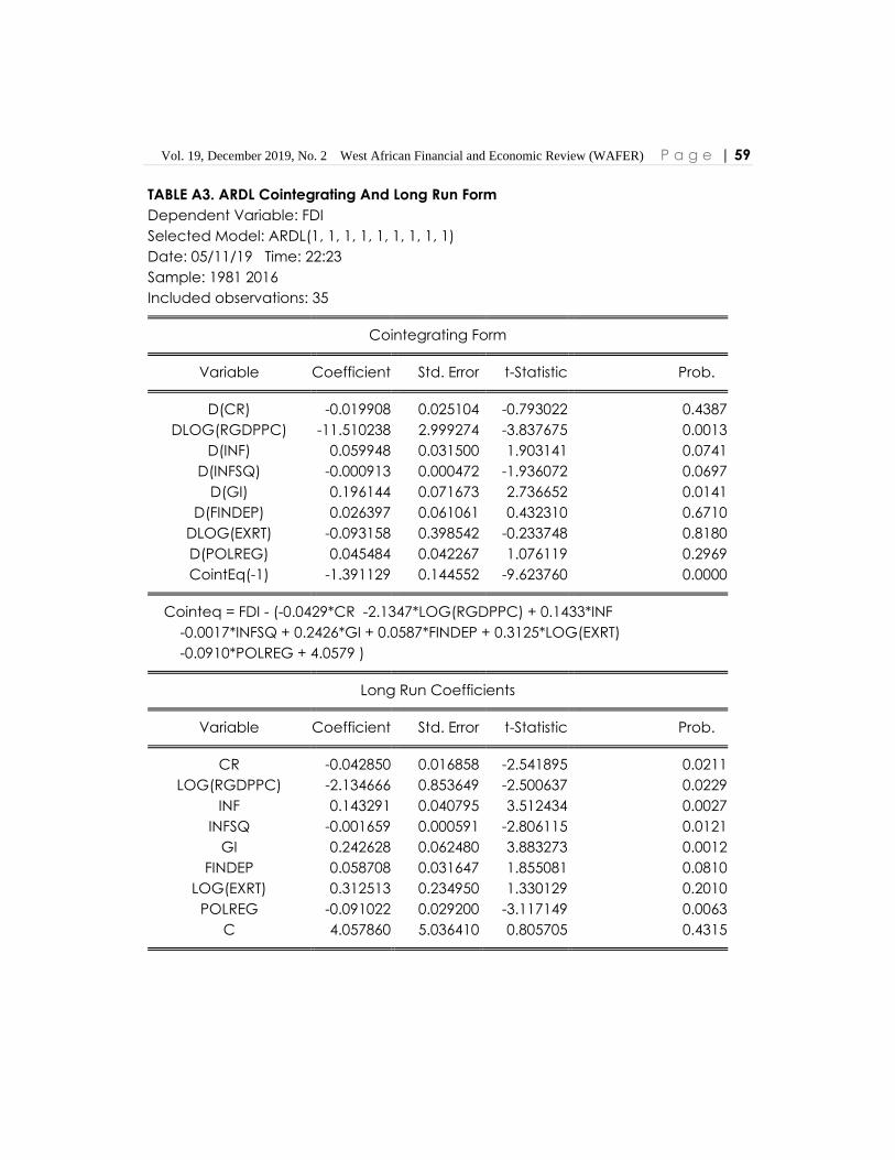
Vol. 19, December 2019, No. 2 West African Financial and Economic Review (WAFER) P a g e | 59
TABLE A3. ARDL Cointegrating And Long Run Form
Dependent Variable: FDI
Selected Model: ARDL(1, 1, 1, 1, 1, 1, 1, 1, 1)
Date: 05/11/19 Time: 22:23
Sample: 1981 2016
Included observations: 35
Cointegrating Form
Variable Coefficient Std. Error t-Statistic Prob.
D(CR) -0.019908 0.025104 -0.793022 0.4387
DLOG(RGDPPC) -11.510238 2.999274 -3.837675 0.0013
D(INF) 0.059948 0.031500 1.903141 0.0741
D(INFSQ) -0.000913 0.000472 -1.936072 0.0697
D(GI) 0.196144 0.071673 2.736652 0.0141
D(FINDEP) 0.026397 0.061061 0.432310 0.6710
DLOG(EXRT) -0.093158 0.398542 -0.233748 0.8180
D(POLREG) 0.045484 0.042267 1.076119 0.2969
CointEq(-1) -1.391129 0.144552 -9.623760 0.0000
Cointeq = FDI - (-0.0429*CR -2.1347*LOG(RGDPPC) + 0.1433*INF
-0.0017*INFSQ + 0.2426*GI + 0.0587*FINDEP + 0.3125*LOG(EXRT)
-0.0910*POLREG + 4.0579 )
Long Run Coefficients
Variable Coefficient Std. Error t-Statistic Prob.
CR -0.042850 0.016858 -2.541895 0.0211
LOG(RGDPPC) -2.134666 0.853649 -2.500637 0.0229
INF 0.143291 0.040795 3.512434 0.0027
INFSQ -0.001659 0.000591 -2.806115 0.0121
GI 0.242628 0.062480 3.883273 0.0012
FINDEP 0.058708 0.031647 1.855081 0.0810
LOG(EXRT) 0.312513 0.234950 1.330129 0.2010
POLREG -0.091022 0.029200 -3.117149 0.0063
C 4.057860 5.036410 0.805705 0.4315
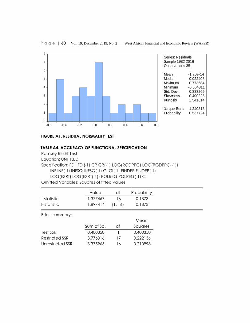
P a g e | 60 Vol. 19, December 2019, No. 2 West African Financial and Economic Review (WAFER)
FIGURE A1. RESIDUAL NORMALITY TEST
TABLE A4. ACCURACY OF FUNCTIONAL SPECIFICATION
Ramsey RESET Test
Equation: UNTITLED
Specification: FDI FDI(-1) CR CR(-1) LOG(RGDPPC) LOG(RGDPPC(-1))
INF INF(-1) INFSQ INFSQ(-1) GI GI(-1) FINDEP FINDEP(-1)
LOG(EXRT) LOG(EXRT(-1)) POLREG POLREG(-1) C
Omitted Variables: Squares of fitted values
Value df Probability
t-statistic 1.377467 16 0.1873
F-statistic 1.897414 (1, 16) 0.1873
F-test summary:
Sum of Sq. df
Mean
Squares
Test SSR 0.400350 1 0.400350
Restricted SSR 3.776316 17 0.222136
Unrestricted SSR 3.375965 16 0.210998
0
1
2
3
4
5
6
7
8
-0.6 -0.4 -0.2 0.0 0.2 0.4 0.6 0.8
Series: ResidualsSample 1982 2016Observations 35
Mean -1.20e-14Median 0.022408Maximum 0.773684Minimum -0.564311Std. Dev. 0.333269Skewness 0.400228Kurtosis 2.541614
Jarque-Bera 1.240818Probability 0.537724
Vol. 19, December 2019, No. 2 West African Financial and Economic Review (WAFER P a g e | 61
MONETARY POLICY EFFECTIVENESS IN AFRICA: DOES TRADE OPENNESS MATTER?
Ekpeno L. Effiong*1 Akpan H. Ekpo1, and Alvin G. Johnson2
Abstract: This paper investigates the effect of trade openness on the impact of
monetary policy on output growth and inflation in Africa using a panel data regression-
based approach with annual data from the period 1990-2015 for a panel of 37 African
countries. We find a strong significant relationship between trade openness and
monetary policy effectiveness in Africa. The effects of monetary policy on output
growth is positive and negative for inflation at higher levels of trade openness. This
suggests that trade openness can enhance the effectiveness of monetary policy for
macroeconomic stabilization on the continent. Therefore, monetary authorities in
Africa should place emphasis on the degree of trade openness when designing their
choice of optimal monetary policy.
Keywords: Openness; Monetary Policy; Panel Data Analysis; Africa.
JEL Classification: C33; E52; F41; O55
1.0 Introduction
As a useful tool for macroeconomic stabilization, monetary policy is important for the
purpose of influencing the direction of economic activities. Through various monetary
transmission channels (i.e. interest rate, exchange rate, and credit channels),
monetary authorities can use monetary policy to either expand or contract activities
in the real economy depending on the desired macroeconomic objective. For
instance, a monetary expansion often raises both the output and price levels
respectively, while monetary tightening has the opposite effects. However, the debate
on the effects of monetary policy often requires a better understanding of the
underlying factors that influences its effectiveness. So far, several factors such as
industry structure, labour market rigidities, trade openness, domestic financial market
development and globalization have been highlighted as plausible determinants of
the effectiveness of monetary policy (see Bernanke and Gertler, 1995; Walsh, 2005;
Karras, 1999, 2001; Berument and Dogan, 2003; Berument et al., 2007; Carranza et al.,
2010; Cwik et al., 2011; Georgiadis and Mehl, 2016; Ma and Lin, 2016; Ma, 2018). In this
1*Corresponding author’s e-mail: [email protected], Tel.: +234 802 789 0160
Department of Economics,, University of Uyo, Uyo, Nigeria 2 West African Institute for Financial and Economic Management Lagos, Nigeria

62 | P a g e Akpan H. Ekpo, Ekpeno L. Effiong and Alvin G. Johnson
paper, we consider the role of trade openness on the effect of monetary policy on
output growth and inflation in African countries.
In open economy monetary economics, a country's domestic currency (i.e. the
nominal exchange rate) is a defining variable in the monetary transmission process,
such that its adjustments do affect the design and conduct of monetary policy. For
instance, international trade activities often have an exchange rate pass-through
effect in an economy. Here, the impact of trade openness on the effects of monetary
policy depends on the manner in which the fluctuations in the exchange rate
influences input prices, inflationary expectations and wage formation. For example,
an exchange rate depreciation following a domestic monetary expansion often leads
to higher input prices, higher prices for imported consumer goods and higher wage
demands. In relatively more open economies, these supply-side mechanisms reduce
the impact of monetary policy on output and increase the impact of monetary policy
on consumer prices (see Bryant et al. 1988; and Karras (1999, 2001). In other words,
monetary expansion is supposed to have a weaker effect on output level and a strong
inflationary effect in more open economies. The intuition is straightforward: for more
open economies, expectation of a domestic currency depreciation triggers higher
wage demand which steepens the aggregate supply such that monetary expansion
will be more reflected in prices and less on output (Karras, 1999).3
Another perspective to the debate focuses on the trade openness-inflation
relationship resulting from the absence of pre-commitment in monetary policy.
Building on Romer (1993), the argument is that unanticipated monetary expansion
induces real exchange rate depreciation which, in turn, generates an inefficiently high
inflation. For more open economies faced with a steeper Phillips curve (i.e., a larger
output-inflation trade-off), the incentive to engage in expansionary monetary policy
diminishes with a higher degree of openness. Consequently, inflation is expected to
be lower in more open economies (see also, Lane, 1997). Put differently, the short-term
benefit of an unanticipated monetary expansion is negatively correlated with the
degree of openness such that less expansion will, on average, lower inflation in more
open economies. In all, the theoretical expectation is that the effect of monetary
policy on output diminishes with trade openness; while in the case of inflation, the
3 This is the supply-side effect of monetary expansion in a more open economy. The opposite will
be true for the less open economy. On the other hand, the demand-side effect would depend
on the nature of expenditure-switching between domestic and foreign goods. However, the
assumption is that the demand effect will be similar for both a more open and relatively closed
economies.

Vol. 19, December 2019, No. 2 West African Financial and Economic Review (WAFER P a g e | 63
relationship can be positive or negative to indicate that prices increase or decrease
respectively with an increasing level of openness.
Using annual data for a panel of 37 African countries from the period 1990 to 2015, this
paper investigates the role of trade openness on the effects of monetary policy on
output and inflation. The aim is to examine whether these theoretical effects can be
empirically validated for African countries. A number of reasons motivate our focus on
Africa. First, there is a dearth of empirical evidence on the impact of trade openness
on the effects of monetary policy in Africa. Attempts at investigating the underlying
factors that could influence monetary policy effectiveness on the continent have so
far concentrated on the role of excess liquidity (Saxegaard, 2006), and financial sector
development (Effiong et al., 2017). Hence, there is need to investigate whether
openness to trade influences the effects of monetary policy on output and prices in
Africa. Second, regional integration has been intensified on the continent over the last
three decades with the formation of regional economic communities through the
initiatives of Regional Trade Agreements (RTAs). Recent efforts include the Tripartite
Free Trade Area (TFTA) and the Continental Free Trade Area (CFTA) which are
designed to deepen intra-regional trade and investment for both employment
creation and growth (AEO, 2016).4 These initiatives are expected to enhance regional
economic co-operation and financial market integration among Africa countries, the
realization of which, would lead to the birth of an African Monetary Union. The success
of such macroeconomic interdependence among African economies will no doubt
have implications for the design and conduct of monetary policy on the continent.
The balance of this paper is organised as follows. Section 2 provides a brief survey of
the literature while Section 3 discusses the empirical methodology and data. Section
4 presents the empirical results with a number of robustness checks. Section 5
concludes with the policy implications.
4 The TFTA is the largest free trade zone in Africa, and it comprise of member countries of the
Common Market for Eastern and Southern Africa (COMESA), East African Community (EAC) and
the Southern African Development Community (SADC). Meanwhile, the objective of CFTA is that
it will evolve into an African Economic Community that would reduce the overlaps between
Africa's regional communities.
64 | P a g e Akpan H. Ekpo, Ekpeno L. Effiong and Alvin G. Johnson
2.0 Literature Review
There is an extant literature on the monetary policy transmission mechanism with
specific focus on the empirical effects of monetary policy on aggregate demand (see
Walsh, 2017). Much of the literature on the subject have focussed on the advanced
and emerging economies with the empirical evidence showing that monetary policy
shocks do exert strong and systematic effects on both output and prices, thereby
confirming the effectiveness of monetary policy in influencing aggregate demand. For
developing countries, the effectiveness of monetary policy has been limited. For
instance, in a survey on the effectiveness of monetary policy transmission in low-
income countries, Mishra and Montiel (2013) found no evidence for a strong monetary
transmission. Thus, the important challenge has been that of identifying the means
through which the effectiveness of monetary policy could be enhanced in these
countries. In that respect, research into the determinants of monetary policy
effectiveness have highlighted several factors which include industry structure, labour
market rigidities, trade openness, domestic financial market development and
globalization (see Bernanke and Gertler, 1995; Walsh, 2005; Karras, 1999, 2001;
Berument and Dogan, 2003; Berument et al., 2007; Carranza et al., 2010; Cwik et al.,
2011; Georgiadis and Mehl, 2016; Ma and Lin, 2016; Ma, 2018).
Concentrating on the relationship between trade openness and the effects of
monetary policy on output and prices, Karras (1999) used annual data from 1953-1990
for a panel of 38 countries and finds evidence in support of the theory: the more open
an economy, the smaller (larger) the output (inflation) effects of monetary policy
shocks. Karras (2001) reports similar evidence for the relationship between openness
and the effects of monetary policy on output for eight countries (Australia, Canada,
Germany, Italy, Japan, South Africa, the U.K. and the U.S.A.) using quarterly data from
the period 1960 to 1994. Berument and Dogan (2003) find evidence on the importance
of openness for monetary policy effectiveness in Turkey. Their results show that a
change in money supply will lead to a smaller output, whereas the impact on inflation
is a parallel to Romer’s hypothesis that demonstrates a negative relationship with the
level of openness.
Berument et al. (2007) analysed the effect of openness on the effectiveness of
monetary policy on output growth and inflation for a group of 29 countries using
quarterly data from 1957:2 to 2003:4 on the basis of country-by-country estimations.
They find variations in the effect of openness on monetary policy effectiveness on
output and inflation across countries. Thus, they argued that difference in countries’
characteristics such as exchange rate regimes, the degree of central bank
Vol. 19, December 2019, No. 2 West African Financial and Economic Review (WAFER P a g e | 65
independence, exposure to international financial crises, terms-of-trade shocks,
different monetary policy stance, and the degree of capital controls could affect the
monetary policy transmission process, and thereafter influence the relationship
between openness and monetary policy effectiveness. Isik and Acar (2006) find
empirical support for the theoretical relationship that a higher degree of openness will
dampen the output effects of changes in money supply. Further evidence shows that
monetary policy has limited effect in developing countries than in developed
economies.
Cwik et al. (2011) evaluates the role of trade integration - or openness - for monetary
policy transmission in a medium-scale New Keynesian Dynamic Stochastic General
Equilibrium (DSGE) model with strategic complementarities in price setting. Their
counterfactual simulations show that openness affects monetary transmission
significantly, and that the effect of a monetary policy shock on inflation and output
tend to increase with openness. Coric et al. (2016) investigates the impact of
economic openness and the responsiveness of output to a domestic monetary policy
shock for a sample of 48 developing and developed countries. Using the structural
vector autoregression (SVAR) model, the effects of a monetary policy shock on output
for each country is estimated, and subsequently used in a cross-section regression to
investigate the sources of cross-country variation in the output response to a monetary
policy shock. Their findings indicate that monetary policy shock has on average a
larger effect on output with a higher openness to trade. Other important factors
include the exchange rate regime and banking sector development.
Related to this strand of the literature are other studies that have considered
alternative factors that may influence the effects of monetary policy on output growth
and inflation. For instance, Ma and Lin (2016) investigates the relationship between
financial development and the effectiveness of monetary policy using panel data
from 41 economies. They find that the effects of monetary policy on output and
inflation are significantly and negatively correlated with financial development, which
indicates that the effectiveness of monetary policy declines as the financial system
becomes more developed. Similarly, Ma (2018) investigates how financial
development and financial structure affect the growth effect of monetary policy using
panel data from 49 countries over the period 1980–2014. Evidence from the empirical
analysis show that financial development has a significantly negative impact on the
growth effect of monetary policy. Moreover, the growth effect of monetary policy
tends to be more pronounced as the financial structure of a country becomes more
market-based. Georgiadis and Mehl (2016) investigates the net impact of financial
66 | P a g e Akpan H. Ekpo, Ekpeno L. Effiong and Alvin G. Johnson
globalization on monetary policy effectiveness with evidence suggesting that financial
globalisation has modified the transmission of monetary policy by strengthening the
importance of the exchange rate channel. For example, their estimates show that the
output effect of tightening monetary policy has increased by 25 percent due to
financial globalisation.
Most of the above studies have concentrated on advanced economies with little
research for developing countries in general, and Africa in particular. For Africa,
Saxegaard (2006) examined the relationship within the context of Sub-Saharan Africa
(SSA) and with particular focus on excess liquidity and its consequent effect on
monetary policy effectiveness. The evidence suggests that excess liquidity weakens
the monetary policy transmission mechanism and thus the ability of monetary
authorities to influence demand conditions in the economy. Likewise, Effiong et al.,
(2017) examined the role financial development on monetary policy effectiveness for
Africa. Their evidence suggest that financial development has a weak effect on the
effectiveness of monetary policy which can be attributed to the underdeveloped
nature of the financial sector on the continent. Meanwhile, studies on the role of trade
openness within the context of African countries are non-existent, therefore, this study
seeks to fill the research gap in the literature.
3.0 Econometric Methodology and Data
Following the empirical approach of previous studies (see e.g. Karras, 1999, 2001; Ma
and Lin, 2016), we examine the relationship between a country's degree of trade
openness on the effectiveness of monetary policy in Africa. To that end, the effects of
trade openness on monetary policy must be specified within a tractable econometric
framework. Consequently, we use two standard panel data models for
macroeconomic analysis to demonstrate the effects of trade openness on the impact
of monetary policy on output and inflation as follows:5
Δ𝑦𝑗,𝑡 = 𝛽0 + ∑ 𝛽𝑖𝑦
𝑄
𝑖=1
Δ𝑦𝑗,𝑡−𝑖 + ∑ 𝛽𝑖𝑜𝑖𝑙
𝑅
𝑖=0
Δ𝑂𝐼𝐿𝑗,𝑡−𝑖 + ∑ 𝛽𝑖,𝑗,𝑡𝑚
𝑆
𝑖=0
Δ𝑚𝑗,𝑡−𝑖 + 𝑢𝑗,𝑡𝑦
(1)
5 The literature on monetary policy and the monetary transmission mechanism uses the VAR
methodology to derive impulse response functions (IRFs) of real macroeconomic variables such
as output and prices following an unanticipated monetary policy shock. Its methodological
shortcomings include: identification of the intermediate target of monetary, and exogenous
monetary policy shocks through various identification schemes such as Choleski decompositions
or non-recursive (simultaneous) identification.

Vol. 19, December 2019, No. 2 West African Financial and Economic Review (WAFER P a g e | 67
Δ𝑝𝑗,𝑡 = 𝛾0 + ∑ 𝛾𝑖𝑝
𝑄
𝑖=1
Δ𝑝𝑗,𝑡−𝑖 + ∑ 𝛾𝑖𝑜𝑖𝑙
𝑅
𝑖=0
Δ𝑂𝐼𝐿𝑗,𝑡−𝑖 + ∑ 𝛾𝑖,𝑗,𝑡𝑚
𝑆
𝑖=0
Δ𝑚𝑗,𝑡−𝑖 + 𝑢𝑗,𝑡𝑝
(2)
where 𝑗 and 𝑡 indexes cover countries and time respectively. ∆𝑦 is the output growth
rate, ∆𝑝 is the inflation rate, ∆𝑚 is the money growth rate, and ∆𝑂𝐼𝐿 is the growth rate
of real oil prices which is included as a proxy for possible supply shocks. As in Karras
(1999), Eq. (1) and (2) represents the reduced-form expressions for output growth and
inflation with 𝛽’s and 𝛾’s as coefficients; and 𝑢𝑗,𝑡𝑦
and 𝑢𝑗,𝑡𝑝
as the output and inflation
shocks respectively, which are modelled as 𝑢𝑗,𝑡𝑦
= 𝑢𝑗𝑦
+ 𝑤𝑗,𝑡𝑦
and 𝑢𝑗,𝑡𝑝
= 𝑢𝑗𝑝
+ 𝑤𝑗,𝑡𝑝
, where 𝑢𝑗𝑦
and 𝑢𝑗𝑝 denote country fixed effects.
To capture the impact of trade openness on the effects of money growth on output
and inflation, an interaction term for trade openness is incorporated in the following
manner (see Karras, 1999; Berument and Dogan, 2003; Ma and Lin, 2016):
𝛽𝑗,𝑡−1𝑚 = 𝜗𝑖
𝑚 + 𝜗𝑖𝑜𝑜𝑝𝑒𝑛𝑗,𝑡−1 (3)
𝛾𝑗,𝑡−1𝑚 = 𝜙𝑖
𝑚 + 𝜙𝑖𝑜𝑜𝑝𝑒𝑛𝑗,𝑡−1 (4)
where 𝑜𝑝𝑒𝑛𝑗,𝑡 is a measure of trade openness in country 𝑗 at time 𝑡, while 𝜗s and 𝜙s are
the parameters. Incorporating Eq.(3) into Eq.(1), gives the output equation which
measures the effect of trade openness on the money growth and output growth
relationship; while the inflation equation is obtained by incorporating Eq.(4) into Eq.(2),
to measure the effect of trade openness on the money growth and inflation
relationship. The resulting equations are as follows:
Δ𝑦𝑗,𝑡 = 𝛽0 + ∑ 𝛽𝑖𝑦
𝑄
𝑖=1
Δ𝑦𝑗,𝑡−𝑖 + ∑ 𝛽𝑖𝑜𝑖𝑙
𝑅
𝑖=0
Δ𝑂𝐼𝐿𝑗,𝑡−𝑖 + ∑(𝜗𝑖,𝑗,𝑡𝑚
𝑆
𝑖=0
Δ𝑚𝑗,𝑡−𝑖 + 𝜗𝑖𝑜𝑚𝑜𝑝𝑒𝑛𝑗,𝑡−1Δ𝑚𝑗,𝑡−1)
+ 𝑢𝑗,𝑡𝑦
(5)
Δ𝑝𝑗,𝑡 = 𝛾0 + ∑ 𝛾𝑖𝑝
𝑄
𝑖=1
Δ𝑝𝑗,𝑡−𝑖 + ∑ 𝛾𝑖𝑜𝑖𝑙
𝑅
𝑖=0
Δ𝑂𝐼𝐿𝑗,𝑡−𝑖 + ∑(𝜙𝑖,𝑗,𝑡𝑚
𝑆
𝑖=0
Δ𝑚𝑗,𝑡−𝑖 + 𝜙𝑖𝑜𝑚𝑜𝑝𝑒𝑛𝑗,𝑡−1Δ𝑚𝑗,𝑡−1)
+ 𝑢𝑗,𝑡𝑝
(6)
where 𝑜𝑝𝑒𝑛𝑗,𝑡−1Δ𝑚𝑗,𝑡−1 is the interaction between trade openness and money growth
on output growth and inflation respectively, while all other variables remain as earlier
defined.
The overall strength of monetary policy on output growth and inflation in Eq. (5) and
(6) is easily identified from the sum of the money growth coefficients, ∑ 𝜗𝑖𝑚𝑆
𝑖=0 and
∑ 𝜙𝑖𝑚𝑆
𝑖=0 respectively. For example, monetary policy shocks (say an increase in ∆𝑚𝑡−𝑖)
that leads to larger values in these coefficients would imply a larger overall effect of
68 | P a g e Akpan H. Ekpo, Ekpeno L. Effiong and Alvin G. Johnson
monetary policy on output growth and inflation, whereas the reverse for smaller values
would suggest a dampening effect of monetary policy. Moreover, our main focus
centres on the coefficients of the interaction term between trade openness and
money growth (∑ 𝜗𝑖𝑜𝑚𝑆
𝑖=0 , ∑ 𝜙𝑖𝑜𝑚𝑆
𝑖=0 ), which measures the impact of trade openness on
money growth to output and inflation respectively. Specifically, if the coefficient sign
is positive (negative), then this would imply that more openness to trade will strengthen
(weaken) the effects of monetary policy on output growth and inflation. Meanwhile,
the magnitude of the impact will depend on the coefficient size. For theoretical
consistency, we expect a negative relationship between trade openness and the
effects of monetary policy on output; and a positive relationship between trade
openness and monetary policy effects on inflation as in Karras (1999) or a negative
relationship to fit with Romer’s expectation about the policy choice of monetary
authorities.
Annual data of 37 African countries over the period 1990 to 2015 is used for the
empirical analysis, where countries and time span are selected subject to data
availability. The datasets are retrieved mainly from the World Bank's World
Development Indicators and the IMF's International Financial Statistics except for oil
prices which is sourced from the U.S. Energy Information Administration website. Our
main variables for the analysis include, broad money supply (M2), consumer price
index (CPI), real gross domestic product (GDP), real oil prices (OIL), and measures of
trade openness (open). The first three variables are expressed in growth rates (i.e.,
annual percentage change) as follows respectively:
∆𝑚𝑗,𝑡 = (𝑀2𝑗,𝑡 − 𝑀2𝑗,𝑡−1)/𝑀2𝑗,𝑡−1
∆𝑝𝑗,𝑡 = (𝐶𝑃𝐼𝑗,𝑡 − 𝐶𝑃𝐼𝑗,𝑡−1)/𝐶𝑃𝐼𝑗,𝑡−1
∆𝑦𝑗,𝑡 = (𝐺𝐷𝑃𝑗,𝑡 − 𝐺𝐷𝑃𝑗,𝑡−1)/𝐺𝐷𝑃𝑗,𝑡−1
We use as a measure of trade openness the sum of import and export as a fraction of
GDP:
𝑂𝑃𝐸𝑁𝑗,𝑡 = (𝐼𝑀𝑗,𝑡 + 𝐸𝑋𝑗,𝑡)/𝐺𝐷𝑃𝑗,𝑡. Alternatively and for robustness checks, imports as a
fraction of GDP (𝐼𝑀𝑗,𝑡/𝐺𝐷𝑃𝑗,𝑡) is also used. Lastly, we deflate U.S. dollar oil prices by the
U.S. implicit price deflator to obtain the real oil prices.
Table 1 shows the list of the 37 African economies and their country averages over the
sample period for each measure of inflation, output growth, money growth and the
trade openness indices. As evident from Table 1, substantial variation exists across

Vol. 19, December 2019, No. 2 West African Financial and Economic Review (WAFER P a g e | 69
countries. For instance, average annual output growth rate ranged from a minimum
of 0.49% in Central African Republic to a maximum of 21.071% in Equatorial Guinea;
while the average annual rate of inflation ranged from 2.694% in Senegal to 40.278%
in Sudan. Also, the annual money growth ranged from 6.607% in the Central African
Republic to 46.648% in Guinea Bissau.
Table 1: Sample Means (1990-2015)
Country ∆𝑦 ∆𝑝 ∆𝑚 𝑜𝑝𝑒𝑛1 𝑜𝑝𝑒𝑛2
1. Algeria 2.885 9.464 16.085 60.097 26.245
2. Benin 4.520 4.414 13.105 57.179 33.832
3. Botswana 4.664 8.905 16.144 96.811 45.662
4. Burkina Faso 5.361 3.178 12.147 41.399 27.514
5. Burundi 1.225 11.448 15.639 36.295 28.319
6. Cabo Verde 7.059 3.642 13.838 90.147 61.003
7. Cameroon 2.604 3.668 7.079 42.158 21.462
8. Central African Rep. 0.490 5.627 6.607 41.385 24.906
9. Chad 5.969 4.241 12.351 67.955 40.635
10. Congo Rep. 3.188 5.155 13.275 126.902 55.335
11. Cote d'Ivoire 2.554 3.903 9.275 78.372 35.559
12. Egypt 4.224 9.178 14.043 49.708 27.710
13. Equatorial Guinea 21.071 5.845 27.306 232.051 147.607
14. Gabon 2.455 2.928 9.069 87.611 31.984
15. Gambia 3.366 5.895 15.948 63.467 38.049
16. Ghana 5.490 20.527 34.369 78.559 46.520
17. Guinea-Bissau 2.285 16.029 46.648 50.427 32.998
18. Kenya 3.612 12.688 16.876 56.426 32.998
19. Madagascar 2.372 12.415 16.706 62.037 37.195
20. Malawi 4.293 21.616 29.776 61.172 36.935
21. Mali 4.439 3.038 11.525 54.765 32.435
22. Mauritius 4.671 6.041 12.623 120.909 63.367
23. Morocco 3.979 2.710 10.192 63.781 35.557
24. Mozambique 7.467 18.782 29.832 71.369 49.641
25. Niger 3.601 2.975 9.816 47.929 30.162
26. Nigeria 5.561 18.886 27.389 56.375 23.165
27. Rwanda 5.519 7.434 16.254 36.409 26.832
28. Senegal 3.535 2.694 9.717 66.457 39.674

70 | P a g e Akpan H. Ekpo, Ekpeno L. Effiong and Alvin G. Johnson
29. Seychelles 3.818 5.063 12.019 141.851 81.978
30. Sierra Leone 2.822 21.420 27.908 53.455 33.629
31. South Africa 2.446 7.364 12.656 52.886 25.843
32. Sudan 4.996 40.278 40.445 27.967 15.543
33. Swaziland 3.887 8.092 12.599 131.74 71.779
34. Tanzania 5.319 13.598 22.753 47.462 30.013
35. Togo 2.773 4.357 9.551 86.673 50.413
36. Tunisia 4.106 4.222 9.793 92.644 48.656
37. Uganda 6.652 10.33 24.841 38.979 25.333
Panel 4.469 9.407 17.465 72.187 40.969
Note: ∆𝑝 is the CPI inflation rate (%),∆𝑦 is the real growth rate of GDP (%),∆𝑚 is the
growth rate of M2 (%),𝑜𝑝𝑒𝑛1 is the sum of import and export as a fraction of GDP,
and 𝑜𝑝𝑒𝑛2 is the ratio of import to GDP.
In addition, trade openness has also varied substantially across African countries. The
sum of imports and exports as a fraction of GDP (i.e. 𝑜𝑝𝑒𝑛1) ranged from a minimum of
27.067% in Sudan to a maximum of 232.051% in Equatorial Guinea. Similar pattern is
observed for import as a fraction of GDP (i.e. 𝑜𝑝𝑒𝑛2). Moreover, the panel average of
72.187% and 40.969% for both measures of trade openness respectively, indicate that
African countries have become more open to international trade with a high import
component within the sample period. Therefore, these variations in trade openness
should lead to considerable differences in the monetary policy effects on output and
inflation across these countries. Also, whether trade openness exert a significant
influence on the monetary policy effects on output growth and inflation in line with
theoretical prediction remains an empirical question within the context of African
countries which this paper intends to validate in the next section.
4.0 Empirical Results
4.1 Main Results
Table 2 reports the estimate between the degree of openness and the effects of
monetary policy on output growth and inflation. This comprise of the estimates for
output growth and inflation regressions respectively with the definition of openness as
the ratio of sum of import and export to GDP. For the estimation, only the first lag of
output growth and inflation as well as the first lag and contemporaneous level of oil
price growth are included in both output growth and inflation regressions respectively.
Moreover, we allow for a richer lag structure of up to three lags for the interactive

Vol. 19, December 2019, No. 2 West African Financial and Economic Review (WAFER P a g e | 71
effect between money growth and openness to trade. Lastly, panel fixed effects
technique is used to estimate all regression equations. This is because of its consistency
under plausible assumptions in the presence of lagged terms of the dependent
variable (see Judge et al., 1985).
As shown from Table 2, output growth and inflation exhibit some persistence as
indicated by the statistically significantly positive AR(1) term and is precisely estimated
in all regressions; higher oil prices are shown to impact output positively at both
contemporaneous level and first lag, whereas it affects inflation negatively across the
inflation regressions with variation in statistical significance. As for the impact of money
growth, though the signs and statistical significance of the estimated coefficients of
Δ𝑚𝑡−𝑖 do change across both output growth and inflation regressions, the cumulative
effect of the sum of money growth coefficients (i.e. ∑ 𝜗𝑖𝑚
𝑖=0 , ∑ 𝜙𝑖𝑚
𝑖=0 ) indicate the
overall strength of monetary expansion, and monetary policy in general. For output
growth, the sum of Δ𝑚𝑡−𝑖 (i.e. ∑ 𝜗𝑖𝑚
𝑖=0 ) are negative and statistically indifferent from zero
except when up to two lags of money growth is included in the output growth
regressions. These suggest that monetary expansion leads to a reduction in the output
level. In the short-run, monetary expansion often leads to a temporary increase in
output level. But, a backward reversal is possible in the long run following adjustments
of the monetary authority. Hence, output level may fall, on average, in the long run.
Meanwhile, the absence of statistical significance across the regressions is consistent
with the money neutrality proposition in the long run. On the other hand, the estimated
coefficients for the sum of the interactive terms of money growth and trade openness
(i.e. ∑ 𝜗𝑖𝑜𝑚
𝑖=0 ), is positive - although quantitatively small - and statistically significant.
This means that there is positive relationship between trade openness and the effect
of monetary policy on output growth such that a given change in money supply
increases the output level in a more open economy. In other words, openness to trade
enhances the effectiveness of monetary policy on output level. While the evidence is
in contrast with the theoretical prediction of a negative relationship, recent studies
show that trade openness contributes to economic growth on the continent (see e.g.,
Brueckner and Lederman, 2015).
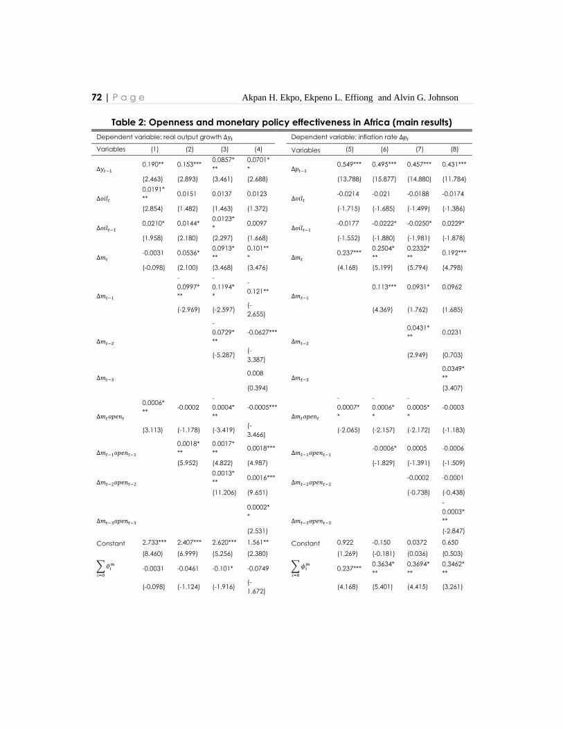
72 | P a g e Akpan H. Ekpo, Ekpeno L. Effiong and Alvin G. Johnson
Table 2: Openness and monetary policy effectiveness in Africa (main results)
Dependent variable: real output growth Δ𝑦𝑡 Dependent variable: inflation rate Δ𝑝𝑡
Variables (1) (2) (3) (4) Variables (5) (6) (7) (8)
Δ𝑦𝑡−1 0.190** 0.153***
0.0857*
**
0.0701*
*
Δ𝑝𝑡−1 0.549*** 0.495*** 0.457*** 0.431***
(2.463) (2.893) (3.461) (2.688) (13.788) (15.877) (14.880) (11.784)
Δ𝑜𝑖𝑙𝑡
0.0191*
** 0.0151 0.0137 0.0123
Δ𝑜𝑖𝑙𝑡 -0.0214 -0.021 -0.0188 -0.0174
(2.854) (1.482) (1.463) (1.372) (-1.715) (-1.685) (-1.499) (-1.386)
Δ𝑜𝑖𝑙𝑡−1 0.0210* 0.0144*
0.0123*
* 0.0097
Δ𝑜𝑖𝑙𝑡−1 -0.0177 -0.0222* -0.0250* 0.0229*
(1.958) (2.180) (2.297) (1.668) (-1.552) (-1.880) (-1.981) (-1.878)
Δ𝑚𝑡 -0.0031 0.0536*
0.0913*
**
0.101**
*
Δ𝑚𝑡 0.237***
0.2504*
**
0.2332*
** 0.192***
(-0.098) (2.100) (3.468) (3.476) (4.168) (5.199) (5.794) (4.798)
Δ𝑚𝑡−1
-
0.0997*
**
-
0.1194*
*
-
0.121**
Δ𝑚𝑡−1
0.113*** 0.0931* 0.0962
(-2.969) (-2.597)
(-
2.655)
(4.369) (1.762) (1.685)
Δ𝑚𝑡−2
-
0.0729*
**
-0.0627***
Δ𝑚𝑡−2
0.0431*
** 0.0231
(-5.287)
(-
3.387)
(2.949) (0.703)
Δ𝑚𝑡−3 0.008
Δ𝑚𝑡−3
0.0349*
**
(0.394) (3.407)
Δ𝑚𝑡𝑜𝑝𝑒𝑛𝑡
0.0006*
** -0.0002
-
0.0004*
**
-0.0005***
Δ𝑚𝑡𝑜𝑝𝑒𝑛𝑡
-
0.0007*
*
-
0.0006*
*
-
0.0005*
*
-0.0003
(3.113) (-1.178) (-3.419)
(-
3.466)
(-2.065) (-2.157) (-2.172) (-1.183)
Δ𝑚𝑡−1𝑜𝑝𝑒𝑛𝑡−1
0.0018*
**
0.0017*
** 0.0018***
Δ𝑚𝑡−1𝑜𝑝𝑒𝑛𝑡−1 -0.0006* 0.0005 -0.0006
(5.952) (4.822) (4.987) (-1.829) (-1.391) (-1.509)
Δ𝑚𝑡−2𝑜𝑝𝑒𝑛𝑡−2
0.0013*
** 0.0016***
Δ𝑚𝑡−2𝑜𝑝𝑒𝑛𝑡−2 -0.0002 -0.0001
(11.206) (9.651) (-0.738) (-0.438)
Δ𝑚𝑡−3𝑜𝑝𝑒𝑛𝑡−3
0.0002*
* Δ𝑚𝑡−3𝑜𝑝𝑒𝑛𝑡−3
-
0.0003*
**
(2.531) (-2.847)
Constant 2.733*** 2.407*** 2.620*** 1.561** Constant 0.922 -0.150 0.0372 0.650
(8.460) (6.999) (5.256) (2.380) (1.269) (-0.181) (0.036) (0.503)
∑ 𝜗𝑖𝑚
𝑖=0
-0.0031 -0.0461 -0.101* -0.0749
∑ 𝜙𝑖𝑚
𝑖=0
0.237*** 0.3634*
**
0.3694*
**
0.3462*
**
(-0.098) (-1.124) (-1.916)
(-
1.672) (4.168) (5.401) (4.415) (3.261)

Vol. 19, December 2019, No. 2 West African Financial and Economic Review (WAFER P a g e | 73
∑ 𝜗𝑖𝑜𝑚
𝑖=0
0.0006*
**
0.0016*
**
0.0026*
** 0.0031*** ∑ 𝜗𝑖
𝑜𝑚
𝑖=0
-
0.0007*
**
-
0.0012*
*
-
0.0012*
*
-
0.0013*
*
(3.113) (5.499) (6.147) (6.870) (-2.065) (2.615) (-2.333) (-2.174)
N 925 925 888 851 925 925 888 851
Adj. R2 0.068 0.164 0.212 0.276 0.472 0.496 0.473 0.401
Note: ∑ 𝜗𝑖𝑚𝑆
𝑖=0 and ∑ 𝜙𝑖𝑚𝑆
𝑖=0 are the sum of the money growth coefficients (∆𝑚𝑡−𝑖) in the output and inflation equation
respectively; ∑ 𝜗𝑖𝑜𝑚𝑆
𝑖=0 and ∑ 𝜙𝑖𝑜𝑚𝑆
𝑖=0 are the sum of the coefficients of the interaction terms (∆𝑚𝑡𝑜𝑝𝑒𝑛𝑡) in the output and
inflation equation respectively with their Wald test F-statistics in the parenthesis, For other coefficients, t-statistics are
reported in parentheses. ***,**,* indicates 1%, 5% and 10% significance level.
As for the case of inflation, the sum of the estimated coefficients of money growth (i.e.
∑ 𝜙𝑖𝑚
𝑖=0 ) are positive and statistically significant across the various lag structure in the
regressions (see Karras, 1999; Berument et al., 2007; Ma and Lin, 2016). The size of these
coefficients are quantitatively higher than those of the output growth regressions, and
is consistent with economic theory prediction that monetary expansion is associated
with higher inflation. However, the sum of the coefficients for the interactive term of
money growth and trade openness (i.e. ∑ 𝜙𝑖𝑜𝑚
𝑖=0 ) is negative and statistically
significant. This means that inflation decreases in a more open economy with
monetary expansion, which fits with Romer’s expectations on the openness-inflation
nexus. In other words, there is a negative relationship between the degree of
openness and the effect of monetary policy on inflation. Therefore, openness to trade
dampens the effect of monetary policy on inflation. Our finding is consistent with
Berument and Dogan (2001), and the recent evidence from Lin et al. (2017) that trade
openness restraints inflation in Sub-Saharan Africa.
Some explanations for our empirical results are worth highlighting. First, higher imports
increases the output level while decreasing prices due to substitution effects
(Berument & Dogan, 2003).6 Africa's export to the world market is mainly dominated
by primary products such as oil, metals etc., and in turn, their import of intermediate
goods (including raw materials) tend to contribute towards output expansion in both
the tradable and non-tradable sectors. With regional integration, increased trade
volume can accelerate output and productivity. Second, openness is likely to reduce
inflation through its positive effect on output in accordance with the ‘new growth
theory’ (Jin, 2000; Ashra, 2002). This link could operate through: (i) increased efficiency
which is likely to reduce costs through changes in composition of inputs procured
domestically and internationally; (ii) better allocation of resources; (iii) increased
capacity utilization; and (iv) an increase in foreign investment. Accordingly,
6 Note that the openness measure increases due to higher imports.
74 | P a g e Akpan H. Ekpo, Ekpeno L. Effiong and Alvin G. Johnson
Cukierman et al. (1992) shows that free trade facilitates convergence in prices of
traded goods across small open economies. Therefore, a lower degree of price
distortion is expected in outward-looking countries. Moreover, inflation - a kind of tax
on domestic currency - is expected to be low in more open economies because of
the relative ease in converting domestic and foreign currencies (Zakaria, 2010). Lastly,
the existence of imperfect competition and nominal price rigidity in the non-tradable
sector can lead to an inverse relationship between openness and inflation (Lane &
Gian, 2006).
4.2 Robustness Checks
As a first step towards validating the above findings, we vary the data frequency to
address possible long-term business cycle effects in the data. Thus, a three-year non-
overlapping country average for each variable is used to re-estimate the output
growth and inflation regressions with the same lag structure as in the above analysis.
Hence, the sample is split into eight data points of the three-year non-overlapping
periods which are 1990-1992, 1993-1995, 1996-1999, 2000-2002, 2003-2005, 2006-2009,
2010-2012, and 2013-2015. The result of the regressions is presented in Table A1 in the
Appendix.
Across both output growth and inflations regressions in Table A1, the sum of the money
growth coefficients has a negative and positive effect on output growth and inflation
respectively. Statistical significance is observed for these coefficients in the output
growth regression with the various lag structure used, and the exception for the
inflation regressions is when the third-lag of money growth is included in the estimation.
However, this evidence does not invalidate the above main findings that monetary
expansion reduces output while increasing inflation. In fact, it reaffirms the importance
of monetary policy as a useful tool for macroeconomic stabilization particularly in the
short run. As for the sum of the interactive term between money growth and openness,
the findings of a positive and negative relationship between openness and the effect
of monetary policy on output and inflation respectively remains unchanged. As an
economy becomes more open, monetary expansion increases output level and
reduces inflation. Therefore, accounting for possible long-term business cycle effects
in the data does not change the reported findings in Table 2 despite the variation in
statistical significance.
For further sensitivity checks, an alternative measure of openness namely, the ratio of
import to GDP (𝑜𝑝𝑒𝑛2) is used. Table A2 presents the estimates for both output growth
and inflation regressions. Looking through the results, the use of import as a fraction of

Vol. 19, December 2019, No. 2 West African Financial and Economic Review (WAFER P a g e | 75
GDP to measure openness does not change the main results but instead it reaffirms
our findings. The sign for the sum of money growth coefficients is negative for output
growth and is statistically significant except at its contemporaneous level in Column
(1). Meanwhile, the effect is positive and statistically significant across the inflation
regressions. Thus, monetary expansion reduces output and increases inflation. On the
other hand, the sum of the interactive term between money growth and openness is
positive for output growth and negative for inflation with all estimates across both
output growth and inflation regressions being statistically significant at the various lag
structure. Therefore, our findings that output level increases while inflation decreases
following monetary expansion in a more open economy is robust with an alternative
measure of openness.
5.0 Conclusion
This paper investigates whether the effects of monetary policy on output growth and
inflation in Africa is influenced by the degree of openness to international trade. Theory
predicts that a monetary expansion dampens output level in a more open economy,
while the effect on inflation is ambiguous as it could be positive in line with Karras
(1999), or negative in support of Romer’s prediction. Annual data for a panel of 37
Africa countries over the period 1990 to 2015 is used to estimate the empirical
accuracy of these theoretical predictions.
Our empirical results show that openness to international trade is an important
determinant of monetary policy effectiveness in Africa. Specifically, openness
enhances the effect of monetary policy on output. Put differently, the effect of a
monetary expansion accelerates output growth as the level of openness increases.
This is contrary to the theoretical prediction of a negative relationship. On the other
hand, openness dampens the effect of monetary policy on inflation. These suggest a
negative relationship between openness and the effect of a given change in money
supply on inflation, such that an increase in openness leads to a decline in inflation.
Hence, the result supports Romer’s prediction on the openness and inflation
relationship. Our empirical results are robust to varying data frequency so as to
account for business cycle effects, and with an alternative measure of trade
openness.
In the light of these empirical results, a direct policy implication is that monetary
authorities in African countries should keep watch on the degree of trade openness
when designing their choice of optimal monetary policy. This is paramount since trade
openness is positively related with output level, while negatively related to inflation.

76 | P a g e Akpan H. Ekpo, Ekpeno L. Effiong and Alvin G. Johnson
Therefore, monetary authorities should act parallel to Romer’s prediction on openness
and monetary policy. Otherwise, the effects of monetary expansion will be absorbed
by inflation. Furthermore, current efforts at regional integration should be deepened
and sustained, since it encourages capital and labour mobility, enhanced trade
volume, and promotes technological innovation, which ultimately contributes to
output growth and productivity. Also, possible concerns among African countries on
the potential loss of monetary policy independence should be weighed with the
stabilization benefit of output and prices in the proposed African Monetary Union.
Vol. 19, December 2019, No. 2 West African Financial and Economic Review (WAFER P a g e | 77
References
AEO (2016). African Economic Outlook 2016: Sustainable Cities and Structural
Transformation. African Development Bank.
Ashra, S. (2002). Inflation and openness: a case study of selected developing
economies. ICRIER Working Paper No. 84, Indian Council of Research on
International Economic Relations.
Bernanke, B. and Gertler, M. (1995). Inside the black box: the credit channel of
monetary policy transmission. Journal of Economic Perspectives, 9 (4), 27–48.
Berument, H. and Dogan, B. (2003). Openness and the effectiveness of monetary
policy: empirical evidence from Turkey. Applied Economics Letters, 10:217-221.
Berument, H., Konac, N., and Senay, O. (2007). Openness and the effectiveness of
monetary policy: a cross-country analysis. International Economic Journal,
21(4):577-591.
Brueckner, M. and Lederman, D. (2015). Trade openness and economic growth: panel
data evidence from Sub-Saharan Africa. Economica, 82:1302-1323.
Bryant, R., Henderson, D., Holtham, G., Hooper, P., and Symansky, S. (1988) Empirical
Macroeconomics for Interdependent Economies. Washington, D.C.: Brookings
Institution.
Carranza, L., Galdon-Sanchez, J.E. and Gomez-Biscarri, J. (2010). Understanding the
relationship between financial development and monetary policy. Review of
International Economics, 18(5): 849-846.
Coric, B., Malesevic Perovic, L., and Simic, V. (2016). Openness and the strength of
monetary transmission: international evidence. Acta Oeconomica, 66(4):639-
659.
Cukierman, A., Webb, S. B., and Neyapti, B. (1992). Measuring the independence of
central banks and its effect on policy outcomes. World Bank Economic Review,
6(3):353-398.
Cwik, T., Gernot, J. M., and Wolters, M. H. (2011). Does trade integration alter monetary
policy transmission? Journal of Economic Dynamics & Control, 35:545-564.
Effiong, E. L., Esu, G., and Chuku, C. (2017). Financial development and monetary
policy effectiveness in Africa. MPRA Paper No. 79732, Munich Presonal RePEC
Archive.
Georgiadis, G. and Mehl, A. (2016). Financial globalization and monetary policy
effectiveness. Journal of International Economics, 103:200-212.
Isik, N. and Acar, M. (2006). Does the effectiveness of monetary policy on output
depend on openness? Journal of Economic and Social Research, 8(1):1-18.

78 | P a g e Akpan H. Ekpo, Ekpeno L. Effiong and Alvin G. Johnson
Jin, J. C. (2000). Openness and growth: an interpretation of empirical evidence from
East Asian countries. The Journal of International Trade & Economic
Development, 9(1):5-17.
Judge, G., Griffiths, W., Lutkepohl, H., and Lee, T. (1985). The Theory and Practice of
Econometrics. John Wiley Press, New York.
Karras, G. (1999). Openness and the effects of monetary policy. Journal of International
Money and Finance, 18:13-26.
Karras, G. (2001). Openness to trade and the potency of monetary policy: How strong
is the relationship? Open Economies Review, 12:61-73.
Lane, P. R. (1997). Inflation in open economies. Journal of International Economics,
42:327-347.
Lane, P. R. and Gian, M. M. (2006). The external wealth of nations mark II: revised and
extended estimates of foreign assets and liabilities, 1970-2004. IMF Working
Paper 06/69, International Monetary Fund: Washington DC.
Lin, F., Mei, D., Wang, H., and Yao, X. (2017). Romer was right on openness and inflation:
evidence from Sub-Saharan Africa. Journal of Applied Economics, 20(1):121-
140.
Ma, Y. and Lin, X. (2016). Financial development and the effectiveness of monetary
policy. Journal of Banking & Finance, 68:1-11.
Ma, Y. (2018). Financial development, financial Structure, and the growth effect of
monetary policy: international evidence. Global Economic Review, 47(4):395-
418.
Mishra, P. and Montiel, P. (2013). How effective is monetary transmission in low-income
countries? A survey of the empirical evidence. Economic Systems, 37:187-216.
Romer, D. (1993). Openness and inflation: theory and evidence. Quarterly Journal of
Economics, 108:869-903.
Saxegaard, M. (2006). Excess liquidity and effectiveness of monetary policy: evidence
from Sub-Saharan Africa. IMF Working Paper No. 06/115, International
Monetary Fund: Washington, DC.
Walsh, C. (2005). Labour market search, sticky prices, and interest rate policies. Review
of Economic Dynamics, 8 (4), 829–849.
Walsh, C. (2017). Monetary Theory and Policy. Fourth Edition. Cambridge MA: MIT Press.
Zakaria, M. (2010). Openness and inflation: evidence from time series data. Dogus
Universitesi Dergisi, 11(2):313-322.

Vol. 19, December 2019, No. 2 West African Financial and Economic Review (WAFER P a g e | 79
APPENDIX
Table A1: Robustness to long-term panel average (three-year averages)
Dependent variable: real output growth Δ𝑦𝑡 Dependent variable: inflation rate Δ𝑝𝑡
Variables (1) (2) (3) (4) Variables (5) (6) (7) (8)
Δ𝑦𝑡−1 0.0444 -0.119 -0.0484 -0.0043
Δ𝑝𝑡−1
0.216**
* 0.182** 0.193*** -0.012
(1.239) (-0.798) (-0.819)
(-
0.032)
(2.827) (2.047) (2.896)
(-
0.115)
Δ𝑜𝑖𝑙𝑡
0.0366** 0.0341* 0.0211 0.0324*
Δ𝑜𝑖𝑙𝑡
-
0.121**
*
-
0.120*** -0.0087 -0.0004
(2.247) (1.953) (1.297) (1.945)
(-
3.976) (-3.886) (0.361)
(-
0.018)
Δ𝑜𝑖𝑙𝑡−1 0.0056 0.0222 0.0139
0.0357*
*
Δ𝑜𝑖𝑙𝑡−1 -0.112* -0.111* 0.0295 0.0282
(0.369) (1.219) (0.943) (2.141)
(-
1.984) (-1.887) (0.735) (0.739)
Δ𝑚𝑡 -0.206**
-
0.188***
-
0.177*** -0.066
Δ𝑚𝑡
0.518**
* 0.476*** 0.0741 -0.0467
(-2.539) (-3.205) (-4.584)
(-
1.417)
(4.272) (3.848) (1.308)
(-
0.848)
Δ𝑚𝑡−1 -0.0135 0.0154 -0.0574 Δ𝑚𝑡−1 0.0893** 0.0503 0.0614
(-0.397) (0.406)
(-
1.401)
(2.402) (0.653) (0.880)
Δ𝑚𝑡−2 0.0223* -0.0375 Δ𝑚𝑡−2 0.0551 -0.0328
(1.915)
(-
0.825)
(1.020)
(-
0.403)
Δ𝑚𝑡−3 0.0237 Δ𝑚𝑡−3 -0.0265
(1.145)
(-
0.549)
Δ𝑚𝑡𝑜𝑝𝑒𝑛𝑡
0.00347*
**
0.0033**
*
0.0032**
* 0.0014***
Δ𝑚𝑡𝑜𝑝𝑒𝑛𝑡
-
0.0014*
*
-0.0011 0.00005 0.0007
(5.652) (6.156) (8.682) (3.066)
(-
2.091) (-1.633) (0.086) (1.101)
Δ𝑚𝑡−1𝑜𝑝𝑒𝑛𝑡−1
0.0022** 0.0012** 0.0014**
Δ𝑚𝑡−1𝑜𝑝𝑒𝑛𝑡−1
-
0.0007**
*
-0.0003 -0.0002
(2.298) (2.677) (2.705)
(-2.999) (-0.356)
(-
0.515)
Δ𝑚𝑡−2𝑜𝑝𝑒𝑛𝑡−2
-
0.0011**
*
0.0003
Δ𝑚𝑡−2𝑜𝑝𝑒𝑛𝑡−2
0.00005
-
0.0000
2
(-7.395) (0.728)
(0.087)
(-
0.031)
Δ𝑚𝑡−3𝑜𝑝𝑒𝑛𝑡−3 -0.0003
Δ𝑚𝑡−3𝑜𝑝𝑒𝑛𝑡−3
0.0000
4
(-
0.929) (0.129)
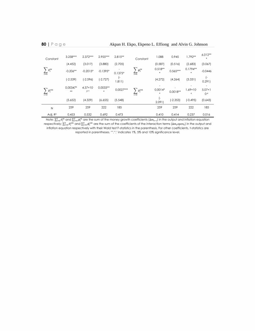
80 | P a g e Akpan H. Ekpo, Ekpeno L. Effiong and Alvin G. Johnson
Constant 3.258*** 2.372*** 2.955*** 2.815**
Constant 1.088 0.945 1.792**
6.012**
*
(4.452) (3.017) (3.880) (2.705) (0.587) (0.516) (2.683) (3.067)
∑ 𝜗𝑖𝑚
𝑖=0
-0.206** -0.2015* -0.1395* -
0.1375* ∑ 𝜙𝑖
𝑚
𝑖=0
0.518**
* 0.565***
0.1794**
* -0.0446
(-2.539) (-2.596) (-2.727)
(-
1.811) (4.272) (4.264) (3.331)
(-
0.291)
∑ 𝜗𝑖𝑜𝑚
𝑖=0
0.00347*
**
4.57×10-
3***
0.0033**
* 0.0027*** ∑ 𝜗𝑖
𝑜𝑚
𝑖=0
-
0.0014*
*
-
0.0018**
-
1.69×10-
4
-
5.07×1
0-4
(5.652) (4.329) (6.655) (5.548)
(-
2.091) (-2.353) (-0.495) (0.643)
N 259 259 222 185 259 259 222 185
Adj. R2 0.453 0.532 0.692 0.473 0.410 0.414 0.237 0.016
Note: ∑ 𝜗𝑖𝑚𝑆
𝑖=0 and ∑ 𝜙𝑖𝑚𝑆
𝑖=0 are the sum of the money growth coefficients (∆𝑚𝑡−𝑖) in the output and inflation equation
respectively; ∑ 𝜗𝑖𝑜𝑚𝑆
𝑖=0 and ∑ 𝜙𝑖𝑜𝑚𝑆
𝑖=0 are the sum of the coefficients of the interaction terms (∆𝑚𝑡𝑜𝑝𝑒𝑛𝑡) in the output and
inflation equation respectively with their Wald test F-statistics in the parenthesis, For other coefficients, t-statistics are
reported in parentheses. ***,**,* indicates 1%, 5% and 10% significance level.
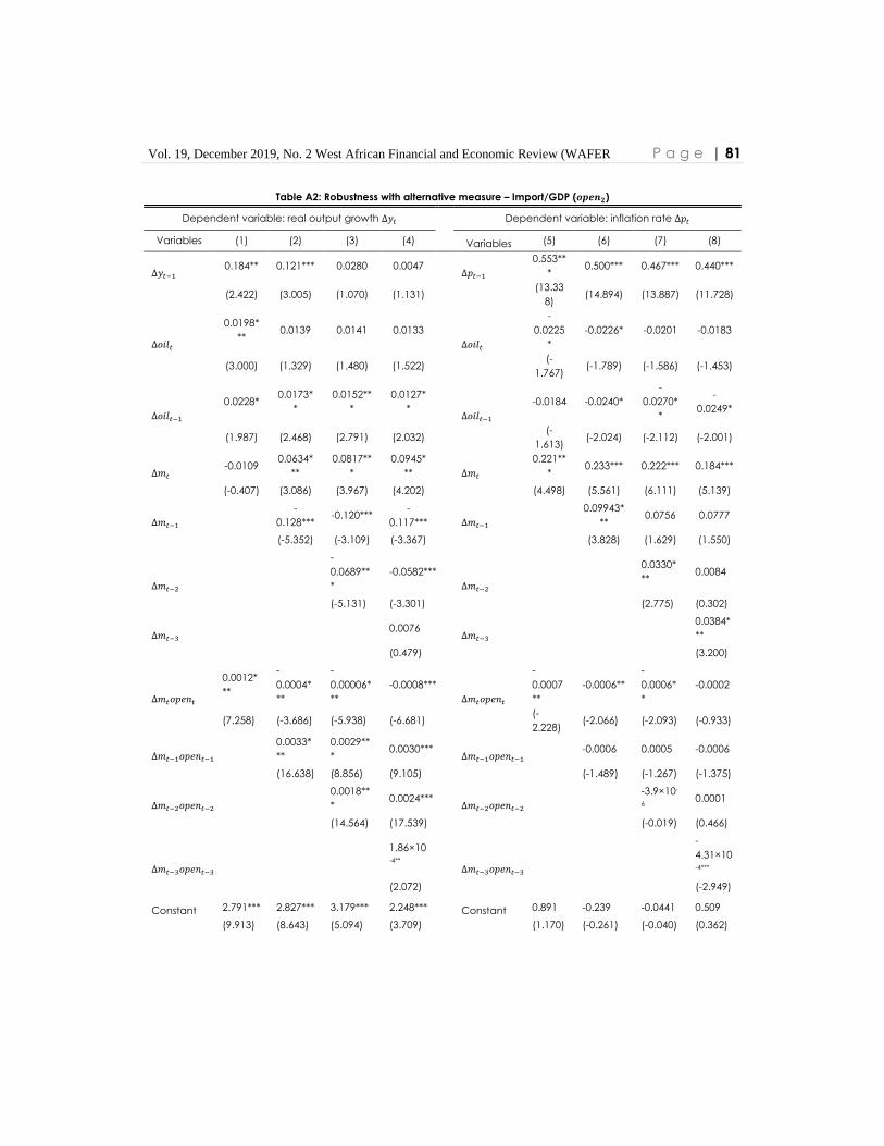
Vol. 19, December 2019, No. 2 West African Financial and Economic Review (WAFER P a g e | 81
Table A2: Robustness with alternative measure – Import/GDP (𝒐𝒑𝒆𝒏𝟐)
Dependent variable: real output growth Δ𝑦𝑡 Dependent variable: inflation rate Δ𝑝𝑡
Variables (1) (2) (3) (4) Variables (5) (6) (7) (8)
Δ𝑦𝑡−1 0.184** 0.121*** 0.0280 0.0047
Δ𝑝𝑡−1
0.553**
* 0.500*** 0.467*** 0.440***
(2.422) (3.005) (1.070) (1.131)
(13.33
8) (14.894) (13.887) (11.728)
Δ𝑜𝑖𝑙𝑡
0.0198*
** 0.0139 0.0141 0.0133
Δ𝑜𝑖𝑙𝑡
-
0.0225
*
-0.0226* -0.0201 -0.0183
(3.000) (1.329) (1.480) (1.522)
(-
1.767) (-1.789) (-1.586) (-1.453)
Δ𝑜𝑖𝑙𝑡−1
0.0228* 0.0173*
*
0.0152**
*
0.0127*
*
Δ𝑜𝑖𝑙𝑡−1
-0.0184 -0.0240*
-
0.0270*
*
-
0.0249*
(1.987) (2.468) (2.791) (2.032)
(-
1.613) (-2.024) (-2.112) (-2.001)
Δ𝑚𝑡 -0.0109
0.0634*
**
0.0817**
*
0.0945*
**
Δ𝑚𝑡
0.221**
* 0.233*** 0.222*** 0.184***
(-0.407) (3.086) (3.967) (4.202) (4.498) (5.561) (6.111) (5.139)
Δ𝑚𝑡−1
-
0.128*** -0.120***
-
0.117***
Δ𝑚𝑡−1
0.09943*
** 0.0756 0.0777
(-5.352) (-3.109) (-3.367) (3.828) (1.629) (1.550)
Δ𝑚𝑡−2
-
0.0689**
*
-0.0582***
Δ𝑚𝑡−2
0.0330*
** 0.0084
(-5.131) (-3.301) (2.775) (0.302)
Δ𝑚𝑡−3 0.0076
Δ𝑚𝑡−3
0.0384*
**
(0.479) (3.200)
Δ𝑚𝑡𝑜𝑝𝑒𝑛𝑡
0.0012*
**
-
0.0004*
**
-
0.00006*
**
-0.0008***
Δ𝑚𝑡𝑜𝑝𝑒𝑛𝑡
-
0.0007
**
-0.0006**
-
0.0006*
*
-0.0002
(7.258) (-3.686) (-5.938) (-6.681)
(-
2.228) (-2.066) (-2.093) (-0.933)
Δ𝑚𝑡−1𝑜𝑝𝑒𝑛𝑡−1
0.0033*
**
0.0029**
* 0.0030***
Δ𝑚𝑡−1𝑜𝑝𝑒𝑛𝑡−1 -0.0006 0.0005 -0.0006
(16.638) (8.856) (9.105) (-1.489) (-1.267) (-1.375)
Δ𝑚𝑡−2𝑜𝑝𝑒𝑛𝑡−2
0.0018**
* 0.0024***
Δ𝑚𝑡−2𝑜𝑝𝑒𝑛𝑡−2
-3.9×10-
6 0.0001
(14.564) (17.539) (-0.019) (0.466)
Δ𝑚𝑡−3𝑜𝑝𝑒𝑛𝑡−3
1.86×10⁻⁴**
Δ𝑚𝑡−3𝑜𝑝𝑒𝑛𝑡−3
-
4.31×10⁻⁴***
(2.072) (-2.949)
Constant 2.791*** 2.827*** 3.179*** 2.248*** Constant 0.891 -0.239 -0.0441 0.509
(9.913) (8.643) (5.094) (3.709) (1.170) (-0.261) (-0.040) (0.362)

82 | P a g e Akpan H. Ekpo, Ekpeno L. Effiong and Alvin G. Johnson
∑ 𝜗𝑖
𝑚
𝑖=0
-0.0109 -
0.0644* -0.1073** -0.0727
∑ 𝜙𝑖
𝑚
𝑖=0
0.221**
*
0.3326**
*
0.3303*
**
0.3089*
**
(-0.407) (-2.014) (-2.432) (-1.906) (4.498) (5.486) (4.415) (3.186)
∑ 𝜗𝑖𝑜𝑚
𝑖=0
0.0012*
**
0.0029*
**
0.0041**
* 0.0048*** ∑ 𝜗𝑖
𝑜𝑚
𝑖=0
-
0.0007
**
-
0.0011**
*
-
0.0011*
*
-
0.0012*
*
(7.258) (13.499) (12.566) (14.029)
(-
2.228) (-2.719) (-2.356) (-2.175)
N 925 925 888 851 925 925 888 851
Adj. R2 0.079 0.237 0.279 0.351 0.471 0.492 0.468 0.396
Note: ∑ 𝜗𝑖𝑚𝑆
𝑖=0 and ∑ 𝜙𝑖𝑚𝑆
𝑖=0 are the sum of the money growth coefficients (∆𝑚𝑡−𝑖) in the output and inflation equation
respectively; ∑ 𝜗𝑖𝑜𝑚𝑆
𝑖=0 and ∑ 𝜙𝑖𝑜𝑚𝑆
𝑖=0 are the sum of the coefficients of the interaction terms (∆𝑚𝑡𝑜𝑝𝑒𝑛𝑡) in the output and
inflation equation respectively with their Wald test F-statistics in the parenthesis, For other coefficients, t-statistics are
reported in parentheses. ***,**,* indicates 1%, 5% and 10% significance level.
P a g e | 83
CREDIT MARKET DEVELOPMENT AND ECONOMIC GROWTH IN LIBERIA: AN
EMPIRICAL INVESTIGATION
Michael D. Titoe Jr.*1, Mussah A. Kamara1
Abstract
The importance of credit market development to economic growth and development
in Liberia has gained traction over time and has been widely discussed in Liberia. This
paper empirically contributes to the discussion by analyzing, within an endogenous
growth framework, the relationship between credit market development and
economic growth in Liberia. An autoregressive distributed lag model is employed to
estimate the relationship, and the findings reveal that in the long run, credit market
development, proxied by domestic credit to private sector as a percentage of gross
domestic product, enhances economic growth which is proxied by the growth of gross
domestic product per capita. The findings also show a unidirectional relationship, with
credit market development Granger causing economic growth in Liberia and the
reverse causality being nonexistent.
JEL Classification: E58, G21, O16
Keywords: Credit Market, Economic Growth, Auto-regressive Distributed Lag,
Cointegration
1.0 Introduction
Credit market plays a major role in economic growth and development of many
economies. Some scholars and researchers have propounded that the development
of credit market can help enhance economic growth and development through
providing credit which helps facilitate entrepreneurship (Schumpeter, 1934; Guiso et
al., 2004), reduce inequality and alleviate poverty (Beck et al., 2007), promote
education (Levine and Rubinstein, 2013), among other positive impacts. Other
researchers have found that a growing economy drives the development of the credit
market (Adamopoulos, 2010; Mishra et al., 2009), while some others have shown that
there exists a two-way causal relationship between credit market development and
economic growth (Greenwood and Jovanovic, 1991; Pradhan, 2009).
1 *Corresponding author’s e-mail: [email protected] 1Research, Policy and Planning Department, Central Bank of Liberia

84 | P a g e Vol. 19, December 2019, No. 2 West African Financial and Economic Review (WAFER)
In Liberia, the credit market has not been fully developed and functional. It is largely
dominated by the banking sector, with a significant informal sector. Some participants
in the market have had complaints on why they think the market has not been
functioning properly. On one hand, some borrowers (particularly small and medium-
sized enterprises) complain of high interest rate and the relatively short period for the
repayment of loans as factors which make loans unhelpful in realizing significant
economic gains, and at times, even make them worse off than they were before
taking the loans. On the other hand, most lenders complain of the issue of non-
performing loans resulting from borrowers defaulting on loan repayments as a major
factor which affects their operations. With these mixed and contending views, there is
a need to investigate the impact of the credit market on economic growth in Liberia.
Against this background, this paper analyzed the credit-growth nexus in Liberia in order
to shed light on what has been the actual impact of the credit market in the Liberian
economy, and thereafter provide recommendations to help inform policy-making on
the development of the country’s credit market. Esso (2010) conducts a cross-country
analysis on the finance-growth nexus in the Economic Community of West African
States (ECOWAS) and tries to address this issue by using 1974-2005 data to do a
bivariate analysis on the relationship between credit to private sector and gross
domestic product per capita in Liberia. The author, however, does not control for other
variables which might affect the relationship between credit to private sector and
growth. This study overcomes such limitation and contributes to the literature on the
credit-growth nexus by utilizing a relatively longer time series on Liberia, and other
control variables, including a polity variable, which controls for the political regime and
authority characteristics of the country.
The rest of the paper is organized as follows. Chapter two presents a review of the
literature, both theoretical and empirical. Chapter three presents the methodology,
detailing the theoretical framework and the empirical model. Chapter 4 presents the
empirical findings and analysis. Chapter five concludes the paper and presents policy
recommendations.
2.0 Literature Review
The literature on credit market development and economic growth provides
theoretical and empirical evidence supporting the view that credit market
development (and in general, financial development) affects economic growth and
development.

Mussah A. Kamara, Michael D. Titoe Jr. P a g e | 85
2.1 Theoretical Literature Review
There are many arguments in the theoretical literature on the importance of credit to
economic growth and development. Some earlier contributors to the literature argued
in favor of the positive role credit market plays in an economy. For example,
Schumpeter (1934) argues that development can be occasioned in an economy
when entrepreneurs, who are innovative, receive credit to invest. Keynes (1937)
emphasizes the need for credit to finance investment which can spur growth and
development. In recent times, Guiso et al. (2004) contend that finance fosters
entrepreneurship, increases market competition by encouraging the entrance of new
firms, and promotes growth.
The credit market being a component of the financial system, significantly contributes
to the overall performance of the system. When the financial system performs well, it
improves the probability of successful innovation and consequently spurs economic
growth (King and Levine, 1993). The financial system also plays an important role in
improving the welfare of people living in poverty. Findings from the work of Beck et al.
(2007) show that credit to private sector alleviates poverty by promoting economic
growth and reducing income inequality which by extension enhances economic
development. The financial system also promotes education by providing access to
finance particularly through the credit market. Levine and Rubinstein (2013) show that
banking sector reforms that ease credit conditions (for example, lower interest rates)
increase college enrollment and hence economic opportunities.
Some authors support the view that there exists a bi-directional relationship between
financial development and growth. For example, Greenwood and Jovanovic (1990)
argue that while economic growth enhances financial development, a developed
financial system also promotes economic growth by allowing more efficient
investments to be undertaken. Blackburn and Hung (1998), also support this view that
there is a two-way causal relationship between growth and financial development.
The quality of financial services significantly impacts economic growth and
development. Levine (2002) supports this argument and confirms the crucial role banks
and markets play in mobilizing and directing savings to the most productive investment
projects. He highlights the importance of the legal system in financial sector
development in terms of protecting the rights of market participants.
As discussed earlier, from a theoretical perspective, credit market has a very germane
role to play in the growth and development of an economy. When the credit market
functions properly, it enhances growth and development; but when it malfunctions,
86 | P a g e Vol. 19, December 2019, No. 2 West African Financial and Economic Review (WAFER)
the economy might be adversely affected. In the literature, a common theme found
in the arguments of some of the proponents of the credit-led growth view is the fact
that credit is needed to facilitate investment which spurs growth and development.
However, the accessibility and affordability of credit are to a great extent dependent
on the nature of the credit market.
2.2 Empirical Literature Review
On the empirical front, there have been some studies that focused on the nexus
between credit market development and economic growth and development. These
studies have used many methodologies and have provided mixed results. For
example, Akpansung and Babalola (2011), using data for the period 1970-2008,
investigate the relationship between banking sector credit and economic growth in
Nigeria. They employ a two-stage least squares approach and find that private sector
credit, a proxy for credit market development, positively impacts economic growth in
Nigeria. Esso (2010) conducts a cross-country analysis to investigate the relationship
between financial development and economic growth in the fifteen ECOWAS
countries. Using a sample ranging from 1974 to 2005 for Liberia, he finds that there exists
a long-run relationship between financial development (proxied by credit to private
sector as a percentage of gross domestic product) and economic growth
(represented by gross domestic product per capita), with there being a one-way
causality running from the former to the latter. Koivu (2002), using a fixed-effect panel
model to analyze the relationship between banking sector development and
economic growth in 25 transition countries for the period 1993-2002, finds that
economic growth does not seem to be accelerated by an increase in the amount of
credit to private sector in those countries. The author argues that banking crises and
soft budget constraints in transition countries have made growth in credit not
sustainable and at times may have even reduced growth.
Adu et al. (2013) use the autoregressive distributed lag approach and principal
component analysis to analyze the financial development-growth nexus in Ghana.
They find that both credit to private sector and total domestic credit enhance growth.
Nkoro and Uko (2013), using vector error correction model (VECM) to analyze data on
Nigeria, find that credit to private sector does not enhance growth. They attribute this
to the problems of high non-performing loans and a deficient legal system which does
not protect contracts in the private sector.
Vazakidis and Adamopoulos (2009) investigate the nexus between credit market
development and economic growth in India for the period 1965-2007. They employ
Mussah A. Kamara, Michael D. Titoe Jr. P a g e | 87
VECM and find that in the short run, an increase in economic growth causes an
increase in bank lending, a proxy they use for credit market development.
Adamopoulos (2010) also analyzes the nexus between credit market development
and economic growth in Spain for the period ranging from 1976 to 2007 using VECM.
He finds that in the short run, economic growth induces an increase in bank lending.
Mishra et al. (2009) use a vector autoregression (VAR) framework and find that
economic growth positively affects credit market development in India.
Pradhan (2009) uses a multivariate VAR model to analyze the relationship between
financial development and economic growth in India. He finds that there exists two-
way causality between economic growth and bank credit. Cappiello et al. (2010) find
that changes in the supply of credit, with regards to volumes and credit standards
applied on loans provided to enterprises, significantly impact real economic activity in
the euro area.
Kar and Pentecost (2000) analyze the nexus between financial development and
growth in Turkey and find that the choice of proxy for financial development
determines the direction of causality between financial development and economic
growth. When private sector credit is considered as a proxy, growth seems to drive
financial development.
3.0 METHODOLOGY
3.1 Theoretical Framework
Following the works of Pagano (1993) and Bailliu (2000), this study adopts an
endogenous growth model to analyze the nexus that exists between credit market
development and economic growth in Liberia. For a closed-economy, the model is
specified as:
𝑌𝑡 = 𝐴𝐾𝑡 (1)
where 𝑌𝑡, A and Kt are national output, total factor productivity, and capital stock,
respectively.
In each period, capital stock is assumed to depreciate at a rate of δ. Hence, gross
investment is given by:
𝐼𝑡 = 𝐾𝑡+1 − (1 − 𝛿)𝐾𝑡 (2)
Through financial intermediation in the credit market, savings are transformed into
investment by financial intermediaries who take from each dollar saved a fraction, 1-

88 | P a g e Vol. 19, December 2019, No. 2 West African Financial and Economic Review (WAFER)
θ, as service fee (or say, transcation cost), and make available θ for investment. It then
follows that equilibrium is attained in the market when net savings and gross investment
are equal such that:
𝜃𝑆𝑡 = 𝐼𝑡 (3)
Making use of equations (1), (2) and (3) and dropping the time subscripts, growth rate
of output at steady state, 𝑔, with financial intermediation is given by:
𝑔 = 𝐴 (𝐼
𝑌) − 𝛿 = 𝐴𝜃𝑠 − 𝛿 (4)
where s is the gross savings rate. Equation (4) shows that economic growth can be
affected by credit market development based on how efficiently financial
intermediation directs savings and capital to investment. For example, it is expected
that the more intermediation banks do, the more efficient they become at doing so,
and thus, transaction cost is reduced. A reduced transaction cost would mean that
the fraction of savings available for investment is increased, thereby resulting to an
increase in 𝑔 in equation (4).
An improvement in capital allocation leads to a rise in overall productivity, 𝐴, and this
drives higher growth. This happens because as financial institutions do more
intermediation, they become better able to assess various investment projects and
choose those with better returns.
Assume that the economy receives international capital inflows (for example, through
foreign direct investment). In this case, higher net inflows of capital in addition to
domestic savings would provide increased funds to facilitate investment. Thus,
equilibrium in the market becomes:
𝜃∗(𝑆𝑡 + 𝐶𝐼𝑡) = 𝐼𝑡∗ (5)
where 𝐶𝐼𝑡 is capital inflows (in this case, from foreign direct investment), and * shows
the presence of international factors. By substituting equation (5) into (4), the steady-
state growth rate is given by:
𝑔∗ = 𝐴∗ 𝐼∗
𝑌− 𝛿 = 𝐴∗𝜃∗ (𝑆+𝐶𝐼)
𝑌− 𝛿 = 𝐴∗𝜃∗𝑠∗ − 𝛿 (6)
According to Bailliu (2000), a comparison of equations (4) and (6) shows that capital
inflows can lead to growth if they increase financial intermediation; if they occasion

Mussah A. Kamara, Michael D. Titoe Jr. P a g e | 89
investments which produce positive spillovers; and primarily, if they cause investment
rate to increase such that 𝑔∗ is greater than 𝑔 when 𝑠∗ is greater than 𝑠, other things
being equal. However, for 𝑠∗ to be greater than 𝑠, net capital inflows should be used
to finance investments which do not crowd out domestically financed investments.
3.2 Empirical Model
Following the work of Jalil and Feridun (2011) who built on the work of Christopoulos
and Tsionas (2004) to transit from the theoretical model to an empirical specification,
the following equation is specified:
𝐿𝐺𝐷𝑃𝑃𝐶𝑡 = 𝛽0 + 𝛽1𝐶𝑅𝐸𝐷𝐼𝑇𝑡 + 𝛽2𝐼𝑁𝐹𝐿𝑡 + 𝛽3𝑇𝑅𝑂𝑃𝑡 + 𝛽4𝐹𝐷𝐼𝑡 + 𝛽5𝑃𝑂𝐿𝐼𝑇𝑌𝑡 + 𝑢𝑡 (7)
where 𝐺𝐷𝑃𝑃𝐶 is the log of gross domestic product (GDP) per capita; 𝐶𝑅𝐸𝐷𝐼𝑇 represents
credit market development; 𝐼𝑁𝐹𝐿 represents the rate of inflation; 𝑇𝑅𝑂𝑃 represents
trade openness; 𝐹𝐷𝐼 represents foreign direct investment; 𝑃𝑂𝐿𝐼𝑇𝑌 represents polity
score; and 𝑢𝑡 is the error term.
To estimate the equation specified in equation (7), this study employs the Auto-
regressive Distributed Lag (ARDL) estimation approach, following Pesaran et al. (2001).
The ARDL approach is appropriate in situation where the variables are integrated of
different orders, namely zero (0) and one (1); and it can be specified as follows:
𝛥𝐿𝐺𝐷𝑃𝑃𝐶𝑡 = 𝛼0 + ∑ 𝛼1𝑖𝛥𝐿𝐺𝐷𝑃𝑃𝐶𝑡−𝑖
𝑝
𝑖=0
+ ∑ 𝛼2𝑖𝛥𝐶𝑅𝐸𝐷𝐼𝑇𝑡−𝑖
𝑝
𝑖=0
+ ∑ 𝛼3𝑖𝛥𝐼𝑁𝐹𝐿𝑡−𝑖
𝑝
𝑖=0
+ ∑ 𝛼4𝑖𝛥𝑇𝑅𝑂𝑃𝑡−𝑖
𝑝
𝑖=0
+ ∑ 𝛼5𝑖𝛥𝐹𝐷𝐼𝑡−𝑖
𝑝
𝑖=0
+ ∑ 𝛼6𝑖𝛥𝑃𝑂𝐿𝐼𝑇𝑌𝑡−𝑖
𝑝
𝑖=0
+ 𝛼7𝐿𝐺𝐷𝑃𝑃𝐶𝑡−1
+ 𝛼8𝐶𝑅𝐸𝐷𝐼𝑇𝑡−1 + 𝛼9𝐼𝑁𝐹𝐿𝑡−1 + 𝛼10𝑇𝑅𝑂𝑃𝑡−1 + 𝛼11𝐹𝐷𝐼𝑡−1 + 𝛼12𝑃𝑂𝐿𝐼𝑇𝑌𝑡−1
+ 𝑢𝑡 (8)
where 𝛼1, 𝛼2, 𝛼3, 𝛼4, 𝛼5, and 𝛼6 are parameters representing short-run dynamics of the
model, and 𝛼7, 𝛼8, 𝛼9, 𝛼10, 𝛼11, and 𝛼12 are parameters representing the long-run
relationship.
90 | P a g e Vol. 19, December 2019, No. 2 West African Financial and Economic Review (WAFER)
3.3 Data and Variable Description
This study utilizes annual time series data for the period 1974-2015 and they are sourced
from the World Bank’s World Development Indicators (2017), the Central Bank of
Liberia’s database and the Polity IV Project (Center for Systemic Peace, 2017). Table 1
describes the variables used in this study.
Table 1: Variable Description
Variable Description
Dependent
LGDPPC The logarithm of gross domestic product per capita
used as a proxy for economic growth/development
Independent
CREDIT Domestic credit to private sector (% of GDP) used as
an indicator of credit market development.
INFL Annual rate of inflation (GDP deflator)
TROP Trade openness proxied by the sum of exports (% of
GDP) and imports (% of GDP)
FDI Foreign direct investment inflows (% of GDP)
POLITY
This variable gives yearly information on the political
regime and authority characteristics of countries. It is
compiled under the Polity IV Project conducted by
the Center for Systemic Peace. It shows the difference
between democracy and autocracy, and it ranges
from +10 (strong democracy) to -10 (strong
autocracy).
4.0 ESTIMATION AND ANALYSIS OF RESULTS
4.1 Unit Root Test
Before estimating the ARDL model, it is necessary that the variables are tested to know
their order of integration as the model is appropriate in the case where variables are
integrated of order zero (0) and order one (1), but not order two (2) and higher. To do
this, the Augmented Dickey Fuller Test is conducted on the variables. The results of the
test reveal that some variables are integrated of order one (that is, become stationary
after first difference) and others are integrated of order zero (that is, stationary at
Mussah A. Kamara, Michael D. Titoe Jr. P a g e | 91
levels), thus confirming the suitability of the ARDL model for this study. The test results
are presented in table 2 below.
Table 2: Augmented Dickey-Fuller Test
Critical Value
Variable Test Statistic 1%
level
5%
level
10%
level
Order of
Integration
LGDPPC -2.115283 -3.610453 -2.938987 -2.607932 I(1)
ΔLGDPPC -3.823343 -3.605593 -2.936942 -2.936942 I(0)
CREDIT -1.158096 -4.226815 -3.536601 -3.200320 I(1)
ΔCREDIT -15.50034 -4.205004 -3.526609 -3.194611 I(0)
INFL -5.115110 -3.600987 -2.935001 -2.605836 I(0)
TROP -1.934094 -3.600987 -2.935001 -2.605836 I(1)
ΔTROP -5.908973 -3.605593 -2.936942 -2.606857 I(0)
FDI -5.367240 -3.600987 -2.935001 -2.605836 I(0)
POLITY -0.400153 -3.600987 -2.935001 -2.605836 I(1)
ΔPOLITY -5.580998 -3.605593 -2.936942 -2.606857 I(0)
4.2 Bounds Test
Since the variables in the model are found to be integrated of different orders, to verify
the presence of cointegration among them, a bounds testing approach is employed
following Pesaran et al. (2001). The null hypothesis under this approach is that there is
no levels relationship. To test this hypothesis, the F-statistic from the bounds test is
compared with the values corresponding to the lower bound, I(0) and the upper
bound, I(1) of the test. If the F-statistic is less than the lower bound value, there is no
rejection of the null hypothesis. If the F-statistic is higher than the upper bound value,
there is a rejection of the null hypothesis. If the F-statistic falls between the lower and
upper bounds, the test is inconclusive. Since the bounds test results presented in table
3 show that the F-statistic is greater than the upper bound value, there is a rejection of
the null hypothesis. Thus, the conclusion is that there exists a level (long-run) relationship
among the variables in the model.
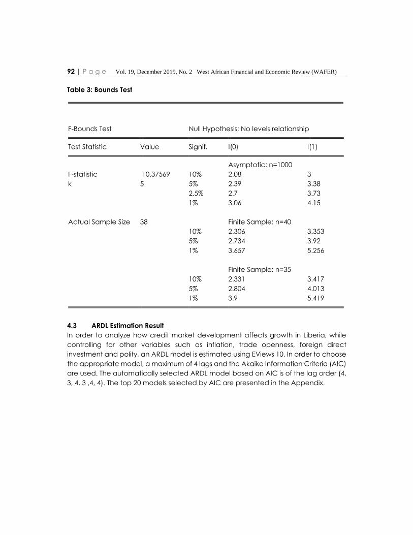
92 | P a g e Vol. 19, December 2019, No. 2 West African Financial and Economic Review (WAFER)
Table 3: Bounds Test
F-Bounds Test Null Hypothesis: No levels relationship
Test Statistic Value Signif. I(0) I(1)
Asymptotic: n=1000
F-statistic 10.37569 10% 2.08 3
k 5 5% 2.39 3.38
2.5% 2.7 3.73
1% 3.06 4.15
Actual Sample Size 38 Finite Sample: n=40
10% 2.306 3.353
5% 2.734 3.92
1% 3.657 5.256
Finite Sample: n=35
10% 2.331 3.417
5% 2.804 4.013
1% 3.9 5.419
4.3 ARDL Estimation Result
In order to analyze how credit market development affects growth in Liberia, while
controlling for other variables such as inflation, trade openness, foreign direct
investment and polity, an ARDL model is estimated using EViews 10. In order to choose
the appropriate model, a maximum of 4 lags and the Akaike Information Criteria (AIC)
are used. The automatically selected ARDL model based on AIC is of the lag order (4,
3, 4, 3 ,4, 4). The top 20 models selected by AIC are presented in the Appendix.
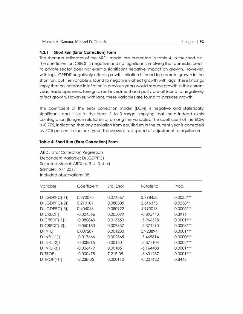
Mussah A. Kamara, Michael D. Titoe Jr. P a g e | 93
4.3.1 Short Run (Error Correction) Form
The short-run estimates of the ARDL model are presented in table 4. In the short run,
the coefficient on CREDIT is negative and not significant, implying that domestic credit
to private sector does not exert a significant negative impact on growth. However,
with lags, CREDIT negatively affects growth. Inflation is found to promote growth in the
short run, but the variable is found to negatively affect growth with lags. These findings
imply that an increase in inflation in previous years would reduce growth in the current
year. Trade openness, foreign direct investment and polity are all found to negatively
affect growth. However, with lags, these variables are found to increase growth.
The coefficient of the error correction model (ECM) is negative and statistically
significant, and it lies in the ideal -1 to 0 range, implying that there indeed exists
cointegration (long-run relationship) among the variables. The coefficient of the ECM
is -0.775, indicating that any deviation from equilibrium in the current year is corrected
by 77.5 percent in the next year. This shows a fast speed of adjustment to equilibrium.
Table 4: Short Run (Error Correction) Form
ARDL Error Correction Regression
Dependent Variable: D(LGDPPC)
Selected Model: ARDL(4, 3, 4, 3, 4, 4)
Sample: 1974 2015
Included observations: 38
Variable Coefficient Std. Error t-Statistic Prob.
D(LGDPPC(-1)) 0.290075 0.076367 3.798458 0.0035***
D(LGDPPC(-2)) 0.210107 0.080305 2.616373 0.0258**
D(LGDPPC(-3)) 0.404046 0.080922 4.993016 0.0005***
D(CREDIT) -0.004566 0.005099 -0.895443 0.3916
D(CREDIT(-1)) -0.080843 0.013550 -5.966378 0.0001***
D(CREDIT(-2)) -0.050180 0.009337 -5.374490 0.0003***
D(INFL) 0.007287 0.001230 5.923894 0.0001***
D(INFL(-1)) -0.017666 0.002365 -7.469814 0.0000***
D(INFL(-2)) -0.008815 0.001501 -5.871104 0.0002***
D(INFL(-3)) -0.006479 0.001051 -6.164408 0.0001***
D(TROP) -0.000478 7.21E-05 -6.631287 0.0001***
D(TROP(-1)) -2.23E-05 0.000110 -0.201622 0.8443

94 | P a g e Vol. 19, December 2019, No. 2 West African Financial and Economic Review (WAFER)
D(TROP(-2)) 0.000369 0.000108 3.418854 0.0066***
D(FDI) -0.003010 0.000286 -10.51016 0.0000***
D(FDI(-1)) 0.004578 0.000527 8.684615 0.0000***
D(FDI(-2)) 0.002539 0.000394 6.449103 0.0001***
D(FDI(-3)) 0.001504 0.000301 4.989111 0.0005***
D(POLITY) -0.056728 0.006912 -8.207282 0.0000***
D(POLITY(-1)) 0.119565 0.010706 11.16829 0.0000***
D(POLITY(-2)) 0.058022 0.014951 3.880816 0.0031***
D(POLITY(-3)) 0.069219 0.013050 5.304340 0.0003***
CointEq(-1) -0.774815 0.071875 -10.77997 0.0000***
R-squared 0.986888 Mean dependent var 0.003806
Adjusted R-
squared 0.969678 S.D. dependent var 0.205297
S.E. of regression 0.035749 Akaike info criterion -3.531717
Sum squared resid 0.020447 Schwarz criterion -2.583641
Log likelihood 89.10263 Hannan-Quinn criter. -3.194399
Durbin-Watson stat 2.277556
Note: *, **, *** indicate that parameter estimates are statistically significant at 10%, 5%
and 1%, respectively.
4.3.2 Long Run (Levels) Equation Form
The levels relationship giving the long-run estimates of the ARDL model are presented
in table 5.
Table 5: Long Run Equation Form
Variable Coefficient Std. Error t-Statistic Prob.
CREDIT 0.148381 0.009422 15.74775 0.0000***
INFL 0.042186 0.005430 7.769524 0.0000***
TROP -0.001468 0.000170 -8.621214 0.0000***
FDI -0.011011 0.002849 -3.865442 0.0031***
POLITY -0.174046 0.012074 -14.41501 0.0000***

Mussah A. Kamara, Michael D. Titoe Jr. P a g e | 95
C 4.936001 0.108929 45.31389 0.0000***
Note: *, **, *** indicate that parameter estimates are statistically significant at 10%, 5%
and 1%, respectively.
In the long run, credit market development is found to enhance economic growth. A
10-percent increase in domestic credit to private sector (% of GDP) drives economic
growth by 1.5 percent. This result is consistent with the credit-led growth view and
confirms findings by Esso (2010) who reveal that there is a long-run relationship
between credit to private sector and growth in Liberia. The result also corroborates
findings by Akpansung and Babalola (2011) and Adu et al. (2013) who reveal that
credit market development drives economic growth in Nigeria and Ghana,
respectively.
Inflation is also found to drive growth in the long run, albeit minimally. A 1-percent
increase in inflation leads to a 0.04-percent GDP growth. This result is in line with findings
by Mallik and Chowdhury (2001) who reveal that inflation positively affects growth in
the long run in four South Asian countries (Bangladesh, India, Pakistan and Sri Lanka).
Trade openness has a very minimal, negative impact on economic growth in Liberia.
A 1-percent increase in trade openness reduces growth by 0.001 percent. This finding
is consistent with findings of other studies. This could be as a result of Liberia exporting
mainly primary commodities with little or no value addition and importing mainly
consumer goods. Hausmann, Hwang, and Rodrik (2007) find that countries with low-
quality products are more likely to be adversely affected by trade openness. Vlastou
(2010) also finds that trade openness negatively affects growth in African countries.
Foreign direct investment is also found to decrease growth in the long run. A 1-percent
increase in FDI inflows (% of GDP) reduces growth by 0.01 percent. This finding
corroborates the view that FDI has sector-specific growth effects, with FDI to primary
sector having negative impact on growth. This is the case in Liberia as most of the FDI
inflows to the country go to the primary sector. Alfaro (2003) finds that FDI flowing to
the manufacturing sector enhances growth while FDI to the primary sector has a
negative effect on growth.
Polity is found to have an adverse effect on economic growth in Liberia. A 1-unit
increase in the polity score occasions a 0.17 percent decline in economic growth in

96 | P a g e Vol. 19, December 2019, No. 2 West African Financial and Economic Review (WAFER)
the long run, revealing that democracy in Liberia is not growth-enhancing. This result
corroborates findings from the work of Tavares and Wacziarg (2001) who show that
democracy negatively affects growth. Barro (1996) and Barro (1999) also argue that
democracy has negative effects on growth through encouraging rich-to-poor
redistributions of income and enhancing the power of interest groups in systems which
have legislative representations.
4.4 Post-estimation Diagnostics
Several post-estimation diagnostic tests verify the robustness and stability of the
estimated ARDL model. The results contained in table 6 below reveal that there are no
heteroskedasticity and serial correlation, and that the residuals are normally distributed
since the null hypotheses of all three tests are not rejected.
Table 6: Post-estimation Tests
Test Null Hypothesis Test Statistic and P-value
Breusch-Pagan-
Godfrey Test for
Heteroskedasticity
Homoskedasticity (or no
heteroskedasticity)
F-statistic = 0.912724
Prob. F(27,10) = 0.6002
Breusch-Godfrey Serial
Correlation LM Test
No serial correlation F-statistic = 2.824819
Prob. F(8,2) = 0.2877
Normality Test Residuals are normally
distributed
Jarque-Bera = 0.260087
Prob. = 0.878057
4.4.1 Stability Diagnostics
To verify the stability of the estimated ARDL model, three tests are conducted. The
Cumulative Sum of Recursive Residuals (CUSUM Test) and the Cumulative Sum of
Squares of Recursive Residuals (CUSUM of Squares Test) show that the model is
dynamically stable and that there is no problem of structural break. The plots of these
stability tests using the 5-percent confidence interval are found in the Appendix.
The results of the Ramsey RESET Test of functional form presented in table 7 below show
that the estimated model is correctly specified since the null hypothesis of the test is
not rejected.
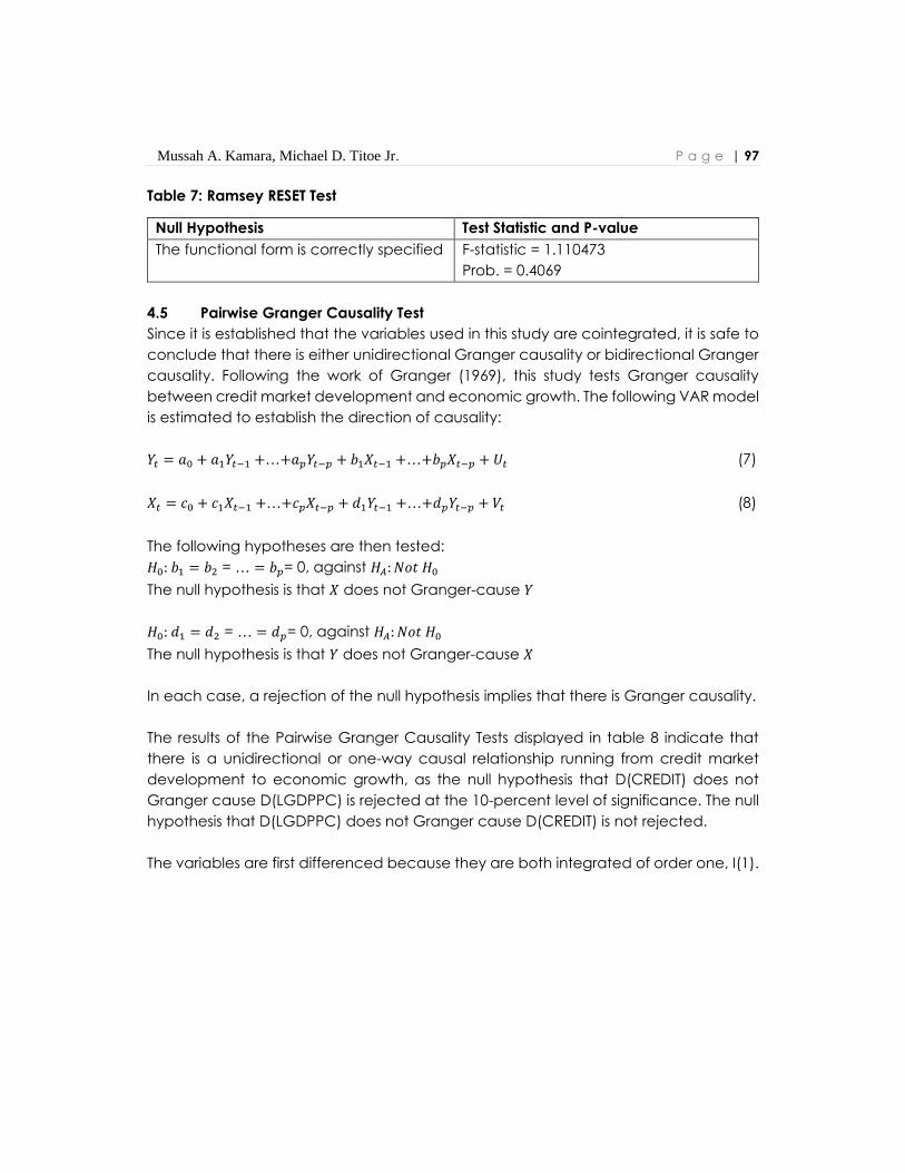
Mussah A. Kamara, Michael D. Titoe Jr. P a g e | 97
Table 7: Ramsey RESET Test
Null Hypothesis Test Statistic and P-value
The functional form is correctly specified F-statistic = 1.110473
Prob. = 0.4069
4.5 Pairwise Granger Causality Test
Since it is established that the variables used in this study are cointegrated, it is safe to
conclude that there is either unidirectional Granger causality or bidirectional Granger
causality. Following the work of Granger (1969), this study tests Granger causality
between credit market development and economic growth. The following VAR model
is estimated to establish the direction of causality:
𝑌𝑡 = 𝑎0 + 𝑎1𝑌𝑡−1 +…+𝑎𝑝𝑌𝑡−𝑝 + 𝑏1𝑋𝑡−1 +…+𝑏𝑝𝑋𝑡−𝑝 + 𝑈𝑡 (7)
𝑋𝑡 = 𝑐0 + 𝑐1𝑋𝑡−1 +…+𝑐𝑝𝑋𝑡−𝑝 + 𝑑1𝑌𝑡−1 +…+𝑑𝑝𝑌𝑡−𝑝 + 𝑉𝑡 (8)
The following hypotheses are then tested:
𝐻0: 𝑏1 = 𝑏2 = … = 𝑏𝑝= 0, against 𝐻𝐴: 𝑁𝑜𝑡 𝐻0
The null hypothesis is that 𝑋 does not Granger-cause 𝑌
𝐻0: 𝑑1 = 𝑑2 = … = 𝑑𝑝= 0, against 𝐻𝐴: 𝑁𝑜𝑡 𝐻0
The null hypothesis is that 𝑌 does not Granger-cause 𝑋
In each case, a rejection of the null hypothesis implies that there is Granger causality.
The results of the Pairwise Granger Causality Tests displayed in table 8 indicate that
there is a unidirectional or one-way causal relationship running from credit market
development to economic growth, as the null hypothesis that D(CREDIT) does not
Granger cause D(LGDPPC) is rejected at the 10-percent level of significance. The null
hypothesis that D(LGDPPC) does not Granger cause D(CREDIT) is not rejected.
The variables are first differenced because they are both integrated of order one, I(1).

98 | P a g e Vol. 19, December 2019, No. 2 West African Financial and Economic Review (WAFER)
Table 8: Pairwise Granger Causality Tests
Sample: 1974 2015
Lags: 3
Null Hypothesis Obs. F-Statistic Prob.
D(CREDIT) does not Granger Cause
D(LGDPPC)
D(LGDPPC) does not Granger Cause
D(CREDIT)
38 2.67417
0.32809
0.0645
0.8050
5.0 Conclusion and Policy Recommendations
This study analyzes, within an endogenous growth framework, the impact of credit
market development on economic growth in Liberia, while controlling for other factors
such as inflation, trade openness, foreign direct investment inflows and polity. An ARDL
model is utilized to estimate the relationship and the findings show that, in the short run,
domestic credit to private sector (% of GDP), the proxy for credit market development,
has no significant impact on growth but adversely affects growth with lags. However,
in the long run, domestic credit to private sector (% of GDP) enhances growth. This
implies that even though the credit market in Liberia is not fully developed and is still
challenged, it has the potential to drive growth and development in the long run if it is
developed and the challenges which affect it are addressed. The results show that a
10-percent increase in domestic credit to private sector (% of GDP) drives growth by
1.5 percent in the long run. This, however, requires proper policy formulation and
implementation by the Government of Liberia (GoL), mainly through the Central Bank
of Liberia.
To ensure an increase in domestic credit to private sector which would enhance
growth, there is a need for GoL to put in place policies to provide protection for both
borrowers and lenders in the credit market. The necessary legal and regulatory
frameworks should be instituted and enforced to ensure that borrowers who acquire
loans from financial institutions (lenders) make repayments as and when due. This
would help to address the problem of non-performing loans. Also, GoL should ensure
that borrowers are not charged excessive interest rates on loans they acquire,
because high interest rates could make loans unattractive or could make borrowers
default on loan repayments. Either of these factors could negatively impact the
volume of credit given out, and by extension, inhibit economic growth.

Mussah A. Kamara, Michael D. Titoe Jr. P a g e | 99
The ongoing reforms of the financial sector by the Central Bank2 is a positive step in the
right direction. However, there is a need for greater support from other players,
including the three (3) branches of Government to ensure full implementation of these
reforms.
2 The reforms, which are meant to enhance the efficiency in the financial sector, include
strengthening the regulation and supervision of financial institutions; deepening the financial
system to cover other financial institutions and agent banking; and improving the national
payment system to include mobile money and digital financial services.

100 | P a g e Vol. 19, December 2019, No. 2 West African Financial and Economic Review (WAFER)
REFERENCES
Adamopoulos, A. (2010b). The Relationship between Credit Market Development and
Economic Growth.” American Journal of Applied Sciences, 7(4), 518-526
Adu, G., Marbuah, G., and Mensah, J. T. (2013). Financial Development and Economic
Growth in Ghana: Does the Measure of Financial Development Matter?.
Review of Development Finance, 3(4), 192-203.
Akpansung, A. O. and Babalola, S. J. (2011). Banking Sector Credit and Economic
Growth in Nigeria: An Empirical Investigation, CBN Journal of Applied Statistics,
ISSN 2476-8472, The Central Bank of Nigeria, Abuja, 2(2), 51-62.
Alfaro, L. (2003). Foreign Direct Investment and Growth: Does the Sector Matter?,
Working Paper, Harvard Business School.
Bailliu, J. N. (2000). Private Capital Flows, Financial Development, and Economic
Growth in Developing Countries. Working Paper 2000-15. Ottawa: Bank of
Canada.
Barro, R. J. (1999). Determinants of Democracy, Journal of Political Economy, 107(S6),
158–183.
Barro, R. J. (1996). Democracy and Growth, Journal of Economic Growth, 1(1), 1–27.
Beck, T., Demirgüç-Kunt, A., and Levine, R. (2007). Finance, Inequality and the
Poor. Journal of Economic Growth, 12(1), 27-49.
Blackburn, K., and Hung, V. T. (1998). A Theory of Growth, Financial Development and
Trade. Economica, 65(257), 107-124.
Cappiello, L., Kadareja, A., Kok, C., and Protopapa, M. (2010). Do Bank Loans and
Credit Standards Have an Effect on Output? A Panel Approach for the Euro
Area. ECB Working Paper No, 1150.
Christopoulos, D. K., and Tsionas, E. G. (2004). Financial Development and Economic
Growth: Evidence from Panel Unit Root and Cointegration Tests. Journal of
Development Economics, 73(1), 55-74.
Esso, L. J. (2010). Cointegrating and Causal Relationship between Financial
Development and Economic Growth in ECOWAS countries. Journal of
Economics and International Finance, 2(4), 036-048.
Granger, C. W. (1969). Investigating Causal Relations by Econometric Models and
Cross-spectral Methods. Econometrica: Journal of the Econometric Society,
37(3), 424-438.
Greenwood, J., and Jovanovic, B. (1990). Financial Development, Growth, and the
Distribution of Income. Journal of Political Economy, 98(5, Part 1), 1076-1107.
Guiso, L., Sapienza, P., and Zingales, L. (2004). Does Local Financial Development
Matter?. The Quarterly Journal of Economics, 119(3), 929-969.

Mussah A. Kamara, Michael D. Titoe Jr. P a g e | 101
Hausmann, R., Hwang, J., and Rodrik, D. (2007). What You Export Matters. Journal of
Economic Growth, 12 (1), 1-25.
Jalil, A., and Feridun, M. (2011). Impact of Financial Development on Economic
Growth: Empirical Evidence from Pakistan. Journal of the Asia Pacific Economy,
16(1), 71-80.
Kar, M., and Pentecost, E. J. (2000) Financial Development and Economic Growth in
Turkey: Further Evidence on the Causality Issue, Economic Research Paper
No.00/27, Department of Economics, Loughborough University.
Keynes, J. M. (1937). The "Ex-ante" Theory of the Rate of Interest. The Economic Journal,
47(188), 663-669.
King, R. G., and Levine, R. (1993). Finance, Entrepreneurship and Growth. Journal of
Monetary Economics, 32(3), 513-542.
Koivu, T. (2002). Do Efficient Banking Sectors Accelerate Economic Growth in Transition
Countries?, Bank of Finland Institute for Economies in Transition, Discussion
Paper No.14.
Levine, R., and Rubinstein, Y. (2014). Liberty for More: Finance and Educational
Opportunities, Cato Papers on Public Policy, Vol. 3.
Levine, R. (2002). Bank-based or Market-based Financial Systems: Which Is Better?
Journal of Financial Intermediation, 11(4), 398-428.
Mallik, G., and Chowdhury, A. (2001). Inflation and Economic Growth: Evidence from
Four South Asian Countries. Asia-Pacific Development Journal, 8(1), 123-135.
Mishra, P. K., Das, K. B., and Pradhan, B. B. (2009). Credit Market Development and
Economic Growth in India. Middle Eastern Finance and Economics, 5(3), 92-
106.
Nkoro, E., and Uko, A. K. (2013). Financial Sector Development-Economic Growth
Nexus: Empirical Evidence from Nigeria. American International Journal of
Contemporary Research, 3(2), 87-94.
Pagano, M. (1993). Financial Markets and Growth: An Overview. European Economic
Review, 37(2-3), 613-622.
Pesaran, M. H., Shin, Y., and Smith, R. J. (2001). Bounds Testing Approaches to the
Analysis of Level Relationships. Journal of Applied Econometrics, 16(3), 289-326.
Pradhan, R. P. (2009). The Nexus between Financial Development and Economic
Growth in India: Evidence from Multivariate VAR Model. International Journal
of Research and Reviews in Applied Sciences, 1(2).
Schumpeter, J. (1934). The Theory of Economic Development. Cambridge, MA.
Harvard University Press.
Tavares, J., and Wacziarg, R. (2001). How Democracy Affects Growth. European
Economic Review, 45(8), 1341-1378.

102 | P a g e Vol. 19, December 2019, No. 2 West African Financial and Economic Review (WAFER)
Vazakidis, A. and Adamopouslos, A. (2009). Credit Market Development and
Economic Growth. American Journal of Economics and Business
Administration, 1(1), 34-40.
Vlastou, I. (2010). Forcing Africa to Open Up to Trade: Is It Worth It? Journal of
Developing Areas, 44(1), 25-39.

Mussah A. Kamara, Michael D. Titoe Jr. P a g e | 103
APPENDIX
Figure 1: Cumulative Sum of Recursive Residuals (CUSUM Test)
-10.0
-7.5
-5.0
-2.5
0.0
2.5
5.0
7.5
10.0
06 07 08 09 10 11 12 13 14 15
CUSUM 5% Significance
Figure 2: Cumulative Sum of Squares of Recursive Residuals (CUSUM of Squares Test)
-0.4
0.0
0.4
0.8
1.2
1.6
06 07 08 09 10 11 12 13 14 15
CUSUM of Squares 5% Significance

104 | P a g e Vol. 19, December 2019, No. 2 West African Financial and Economic Review (WAFER)
Figure 3: Normality Test
0
1
2
3
4
5
6
7
8
9
-0.04 -0.02 0.00 0.02 0.04
Series: Residuals
Sample 1978 2015
Observations 38
Mean -2.11e-16
Median 0.000658
Maximum 0.046344
Minimum -0.048238
Std. Dev. 0.023508
Skewness -0.168665
Kurtosis 2.775336
Jarque-Bera 0.260087
Probabil ity 0.878057
Figure 4: Top 20 ARDL Models
-3.3
-3.2
-3.1
-3.0
-2.9
-2.8
-2.7
-2.6
AR
DL(
4, 3
, 4, 3
, 4, 4
)
AR
DL(
4, 4
, 4, 3
, 4, 4
)
AR
DL(
4, 3
, 4, 4
, 4, 4
)
AR
DL(
4, 4
, 4, 4
, 4, 4
)
AR
DL(
4, 3
, 4, 1
, 4, 4
)
AR
DL(
4, 3
, 4, 2
, 4, 4
)
AR
DL(
4, 4
, 4, 1
, 4, 4
)
AR
DL(
4, 4
, 4, 2
, 4, 4
)
AR
DL(
4, 3
, 4, 3
, 2, 4
)
AR
DL(
4, 3
, 4, 3
, 3, 4
)
AR
DL(
4, 2
, 4, 4
, 0, 4
)
AR
DL(
4, 1
, 4, 3
, 2, 4
)
AR
DL(
4, 1
, 4, 4
, 0, 4
)
AR
DL(
4, 1
, 4, 3
, 4, 4
)
AR
DL(
4, 3
, 4, 4
, 2, 4
)
AR
DL(
4, 2
, 4, 4
, 4, 4
)
AR
DL(
4, 2
, 4, 3
, 4, 4
)
AR
DL(
4, 4
, 4, 3
, 2, 4
)
AR
DL(
4, 1
, 4, 4
, 4, 4
)
AR
DL(
4, 2
, 4, 3
, 0, 4
)
Akaike Information Criteria (top 20 models)
VOLATILITY SPILLOVERS BETWEEN OIL AND STOCK MARKETS: EVIDENCE FROM
NIGERIA AND SOUTH AFRICA
Moses K. Tule1, J.S. Akuns1, L.R. Balakeffi1, C.C. Chiemeke1, S.A, Abdulsalam*2
Abstract
This paper investigates the Volatility spillovers between oil and stock markets: Evidence
from Nigeria and South Africa. The bivariate form of the VAR–CCC-GARCH was
adopted for the study. We find that the shock transmission through oil price changes
tends to affect the stock markets both in Nigeria and South Africa significantly, but the
level of impact tends to be minimal in the latter than the former. We also observed
that the hedging ratios are quite high in South Africa when compared to that of
Nigeria. The observed higher values obtained for the hedge ratios in both countries
suggest that hedging effectiveness relating to both stock and oil markets in both
countries will not deliver the desired outcome to investors. Overall, the paper suggests
several significant implications for making optimal portfolio allocations, engaging in risk
management and forecasting the future path of commodity markets and volatility in
equity for portfolio hedgers.
Keywords: Volatility spillovers, Conditional correlations, Stock indices, Multivariate
GARCH Crude oil prices.
JEL Classifications: C22, C32, G17, G32.
1.0 Introduction
The accelerated growth in liquidity recorded in the commodity markets in recent years
is largely attributable to the influx of investors who are interested in the market purely
for investments with quick returns and not as a means to support economic activity in
the real sector of the beneficiaries (Mensi et al., 2013). The integration, boosted by
developments in technology and innovations, has led to high volatility in major
financial markets, as commodity and equity prices grew more sensitive to innovation
and expectations. The rapid integration of emerging and developing economies
(largely due to financial liberalisation) into the global international markets has
increased significantly, thus fueling volatility (Rasche and Tatom (1977); Hamilton
(1988)).
*Corresponding author’s mail: [email protected] 1 Central Bank of Nigeria 2 West African Monetary Agency

106 | P a g e Vol. 19, December 2019, No. 2 West African Financial and Economic Review (WAFER)
Theoretically, there are many ways through which the oil price movements could have
an impact on the stock returns. For instance, Rasche and Tatom (1977); Hamilton
(1988); Kim and Loungani (1992); Rotemberg and Woodford (1996); and Kilian (2014);
infer that the transmission of oil price shocks to the real economy is via the supply-side
or demand-side channels. The supply-side channel views oil as an intermediate input
in the domestic production process such that increases in the price of oil precipitate
an increase in the cost of production of goods and services. This has inflationary
tendencies which can diminish the purchasing power of consumers. The demand-side
perspective is predicated on the premise that higher oil prices would lead to higher
energy costs which would reduce households’ discretionary income as consumers
would have less money to spend after paying their bills resulting in reduced aggregate
demand.
Nature of oil dependency and persistent oil price shocks has significant implications
for global financial markets, and stock markets in particular. The impact of oil price
shocks on stock markets depends primarily on whether a country is an exporter or
importer of oil and differs from country to country. In oil-exporting countries, a rise in
world oil prices increases the balance of payments’ surplus position, accompanied by
an accumulation of foreign exchange reserves. This leads to an appreciation of the
exchange rate. At the same time, the favourable economic conditions tend to
increase households’ disposable income and corporate profitability, thus increasing
aggregate demand and stock prices. Conversely, falling oil prices would lead to the
depletion of foreign exchange reserves, depreciation of the exchange rate,
inflationary pressures, reduced household disposable income and corporate
profitability, thus, resulting eventually in depressed stock prices. The trend is the reverse
in the case of oil importers (Abdelaziz et al. 2008).
Nigeria has been adjudged to be an emerging economy which though, not fully
integrated into the global economy, but is partially integrated especially through the
financial sector and trade. Also, it is categorised among the top ten oil-producing
countries in the world and net oil exporter hence; any instability in commodity traded
prices, particularly in crude oil, will impact on the country’s macroeconomic
developments with a spillover effect on its financial markets. This provides the rationale
for the choice of Nigeria, as a result, for the study based on the fact that more than
ninety per cent (90%) of the country’s exports are crude oil which generates about
ninety-seven per cent (97%) of the country’s foreign exchange revenue (Gbadebo
2008). It also justifies the basis for an empirical investigation on the correlation between
the stock market and oil price shocks, because the return and spillover transmission
Moses K. Tule, J.S. Akuns, L.R. Balakeffi, , C.C. Chiemeke,S.A, Abdulsalam P a g e | 107
between oil and exchange rate provides reasonable and alternative ideas to investors
on modalities to aid the diversification of their portfolios or hedging of risks. In addition,
the study also introduced the returns and volatility spillover effects in the South African
stock markets in the presence of world oil price shocks to gain insight about the degree
of volatility spillover effect in both oil-based (Nigerian) and none oil-based (South
African) stock markets. Perhaps, more importantly, an empirical investigation and
comparison of the volatility spillovers in Nigeria and South Africa will offer more insights
to investors, including institutional investors and investment managers on how to build
an appropriate assets pricing models, forecast precisely the probable returns and
volatility in both markets and construct an optimal portfolio considering the
interconnectedness and dynamics in world oil prices and stock markets in recent
years. In addition, it will also examine and provide some insight on the optimal weights
and hedge ratios for the choice of holding oil -stock in a portfolio. In order to examine
possible links and the returns and volatility spillover effects in the presence of world oil
price shocks in both Nigerian and South African Stock Markets, a bivariate form of the
VAR–GARCH model was adopted.
Most of the literature reviews, focused largely on traditional developing countries in
Europe, Asia and Gulf countries (Hammaoudeh and Li, 2004;, Kling, 1985; Sardorsky,
1999; and Eryigit, 2009), thus, leaving a gap for economies in the sub-Saharan Africa
(SSA) region including Nigeria. Likewise, most studies on Nigeria focused on the effect
of oil price changes and volatility on output and exchange rate (see Adebiyi et al.,
2009; and Salisu and Mobolaji, 2013). Also, a comparative analysis of the nexus oil price
and stock price between net oil-exporting (Nigeria) and net oil-importing country
(South Africa) in SSA is scanty. This is the motivation for the research.
The study is divided as follows: Section two surveys the extant literature on oil price
shocks and volatility in stock markets. Section three explains the methodology
employed while section four presents the results of the empirical analysis, including the
discussions on the optimal weights and hedge ratios for the choice of holding oil -stock
in a portfolio both in Nigeria and South Africa. Section five discusses the policy
implications of the findings and conclusions.
2.0 Literature Review
Several studies have emerged to empirically confirm or validate the propositions about
the interactions between stock and oil price. These studies have adopted different
methodologies ranging from the VAR-GARCH families (see for example, Arouri, Jouini,
and Nguyen (2011)), SVAR (Basher et al. (2012), fractional co-integration model (Gil-
108 | P a g e Vol. 19, December 2019, No. 2 West African Financial and Economic Review (WAFER)
Alana and Yaya (2014)), co-integration and causality (Apergis and Miller (2009)), etc.
The findings from these various studies have been mixed.
For example, Arouri, Jouini, and Nguyen (2011) found a unidirectional from oil to stock
markets and bi-directional in Europe and the United States, respectively during 1998 -
2009. The bi-directional results were as expected, as increasing oil price affected
consumers’ and investors’ sentiment and demand for financial products. Arouri,
Lahiani, and Nguyen (2011), Masih and Peters (2011) and Lin et al. (2014), find the
existence of substantial return and volatility between world oil prices and stock
markets. Also, Hammoudeh and Aleisa (2004), Hammoudeh and Huimin (2005), Cong,
Wei, Jiao and Fan (2008), Park and Ratti (2008), Donoso (2009), Miller and Ratti (2009),
Apergis and Miller (2009), Filis, Degiannakis and Floros (2011), Narayan and Narayan
(2010), Masih, Peters and De Mello (2011) and Zhang and Chen (2011), find that crude
oil prices have significant positive impact on stock returns. However, Cunado and
Perez de Gracia (2014) and Kang, Ratti and Yoon (2015) find a negative relationship.
In Nigeria, Uwubanmwen and Nguyen (2015), Gil-Alana and Yaya (2014) suggest that
volatility in oil price produces and stimulates stock price volatility in Nigeria. Also,
Boqiang Lin (2014) found significant volatility spillover effect from oil prices to stock
market returns in both Ghana and Nigeria. His study also suggests that the transmission
of volatility seems more apparent from oil to stock than from stock to oil as the case of
Ghana. The study further establishes evidence of the short-term impact of oil price
changes on stock price and shows that conditional volatility changes rapidly as a result
of significant effects of past volatility rather than past news/shocks for all market
returns. The study also shows that there is a slightly more effective hedge in the two
stock markets.
In recent times, a number of papers have extended the analysis of oil price–stock
market nexus by computing the optimal weights and hedging ratios to provide more
insights to investors on how to build appropriate assets pricing models and forecast the
returns and volatility in both markets. Further, in Nigeria, empirical research into the oil
–stock market price nexus is very recent (see Uwubanmwen and Nguyen (2015) for a
survey of the literature) and the issue of both returns and volatility spillover transmission
between oil price and stock market price has remained inconclusive in the literature.
Also, there is a dearth of empirical studies in some emerging countries such as Nigeria
(oil-exporting country) and South Africa (non-oil exporting country) comparing stock
markets and oil price dynamics, extended to estimating optimal weights and hedging
ratios for both countries. These are the contributions of the present study to the existing
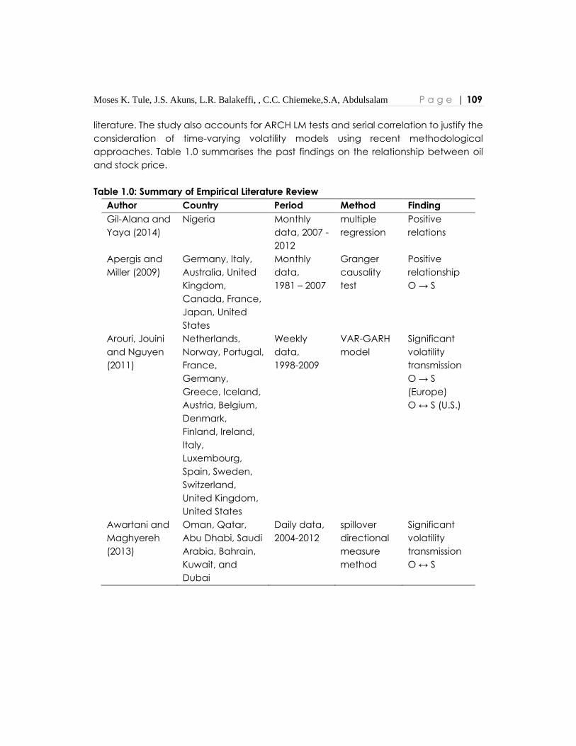
Moses K. Tule, J.S. Akuns, L.R. Balakeffi, , C.C. Chiemeke,S.A, Abdulsalam P a g e | 109
literature. The study also accounts for ARCH LM tests and serial correlation to justify the
consideration of time-varying volatility models using recent methodological
approaches. Table 1.0 summarises the past findings on the relationship between oil
and stock price.
Table 1.0: Summary of Empirical Literature Review
Author Country Period Method Finding
Gil-Alana and
Yaya (2014)
Nigeria Monthly
data, 2007 -
2012
multiple
regression
Positive
relations
Apergis and
Miller (2009)
Germany, Italy,
Australia, United
Kingdom,
Canada, France,
Japan, United
States
Monthly
data,
1981 – 2007
Granger
causality
test
Positive
relationship
O → S
Arouri, Jouini
and Nguyen
(2011)
Netherlands,
Norway, Portugal,
France,
Germany,
Greece, Iceland,
Austria, Belgium,
Denmark,
Finland, Ireland,
Italy,
Luxembourg,
Spain, Sweden,
Switzerland,
United Kingdom,
United States
Weekly
data,
1998-2009
VAR-GARH
model
Significant
volatility
transmission
O → S
(Europe)
O ↔ S (U.S.)
Awartani and
Maghyereh
(2013)
Oman, Qatar,
Abu Dhabi, Saudi
Arabia, Bahrain,
Kuwait, and
Dubai
Daily data,
2004-2012
spillover
directional
measure
method
Significant
volatility
transmission
O ↔ S
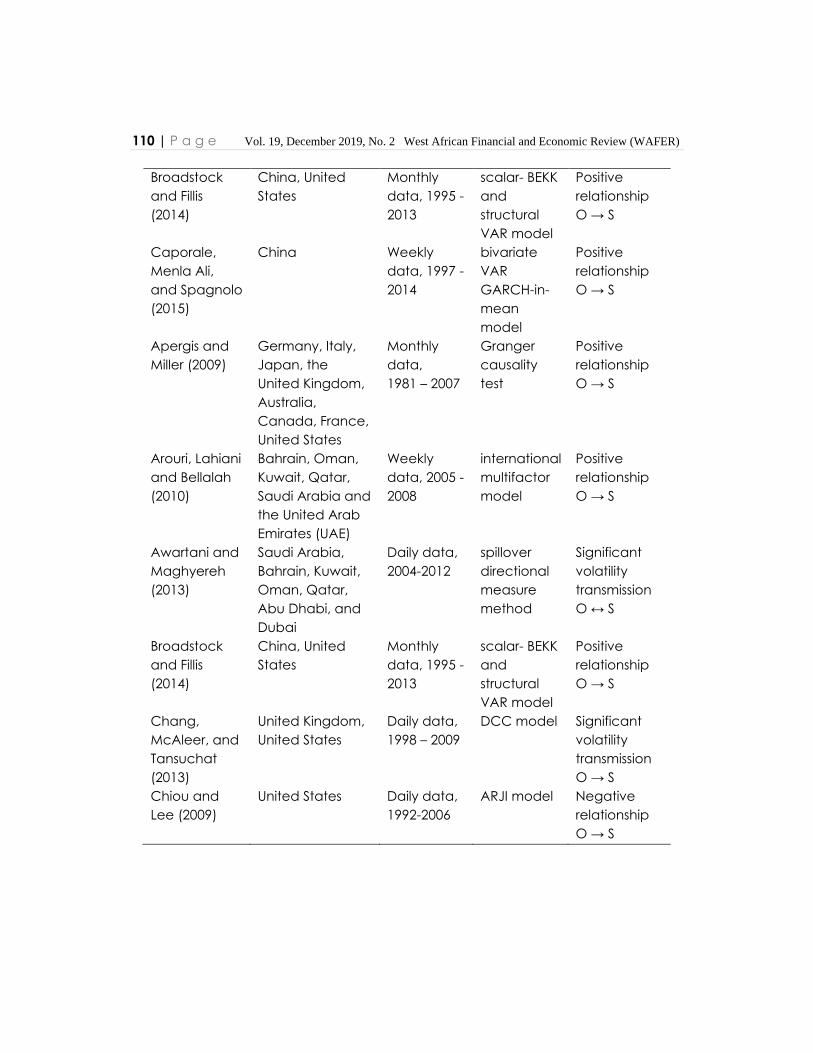
110 | P a g e Vol. 19, December 2019, No. 2 West African Financial and Economic Review (WAFER)
Broadstock
and Fillis
(2014)
China, United
States
Monthly
data, 1995 -
2013
scalar- BEKK
and
structural
VAR model
Positive
relationship
O → S
Caporale,
Menla Ali,
and Spagnolo
(2015)
China Weekly
data, 1997 -
2014
bivariate
VAR
GARCH-in-
mean
model
Positive
relationship
O → S
Apergis and
Miller (2009)
Germany, Italy,
Japan, the
United Kingdom,
Australia,
Canada, France,
United States
Monthly
data,
1981 – 2007
Granger
causality
test
Positive
relationship
O → S
Arouri, Lahiani
and Bellalah
(2010)
Bahrain, Oman,
Kuwait, Qatar,
Saudi Arabia and
the United Arab
Emirates (UAE)
Weekly
data, 2005 -
2008
international
multifactor
model
Positive
relationship
O → S
Awartani and
Maghyereh
(2013)
Saudi Arabia,
Bahrain, Kuwait,
Oman, Qatar,
Abu Dhabi, and
Dubai
Daily data,
2004-2012
spillover
directional
measure
method
Significant
volatility
transmission
O ↔ S
Broadstock
and Fillis
(2014)
China, United
States
Monthly
data, 1995 -
2013
scalar- BEKK
and
structural
VAR model
Positive
relationship
O → S
Chang,
McAleer, and
Tansuchat
(2013)
United Kingdom,
United States
Daily data,
1998 – 2009
DCC model Significant
volatility
transmission
O → S
Chiou and
Lee (2009)
United States Daily data,
1992-2006
ARJI model Negative
relationship
O → S
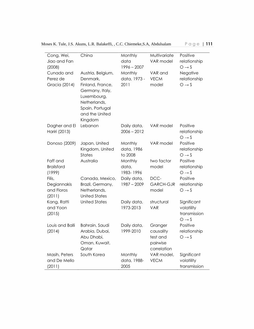
Moses K. Tule, J.S. Akuns, L.R. Balakeffi, , C.C. Chiemeke,S.A, Abdulsalam P a g e | 111
Cong, Wei,
Jiao and Fan
(2008)
China Monthly
data
1996 – 2007
Multivariate
VAR model
Positive
relationship
O → S
Cunado and
Perez de
Gracia (2014)
Austria, Belgium,
Denmark,
Finland, France,
Germany, Italy,
Luxembourg,
Netherlands,
Spain, Portugal
and the United
Kingdom
Monthly
data, 1973 -
2011
VAR and
VECM
model
Negative
relationship
O → S
Dagher and El
Hariri (2013)
Lebanon Daily data,
2006 – 2012
VAR model Positive
relationship
O → S
Donoso (2009) Japan, United
Kingdom, United
States
Monthly
data, 1986
to 2008
VAR model Positive
relationship
O → S
Faff and
Brailsford
(1999)
Australia Monthly
data,
1983- 1996
two factor
model
Positive
relationship
O → S
Filis,
Degiannakis
and Floros
(2011)
Canada, Mexico,
Brazil, Germany,
Netherlands,
United States
Daily data,
1987 – 2009
DCC-
GARCH-GJR
model
Positive
relationship
O → S
Kang, Ratti
and Yoon
(2015)
United States Daily data,
1973-2013
structural
VAR
Significant
volatility
transmission
O → S
Louis and Balli
(2014)
Bahrain, Saudi
Arabia, Dubai,
Abu Dhabi,
Oman, Kuwait,
Qatar
Daily data,
1999-2010
Granger
causality
test and
pairwise
correlation
Positive
relationship
O → S
Masih, Peters
and De Mello
(2011)
South Korea Monthly
data, 1988-
2005
VAR model,
VECM
Significant
volatility
transmission
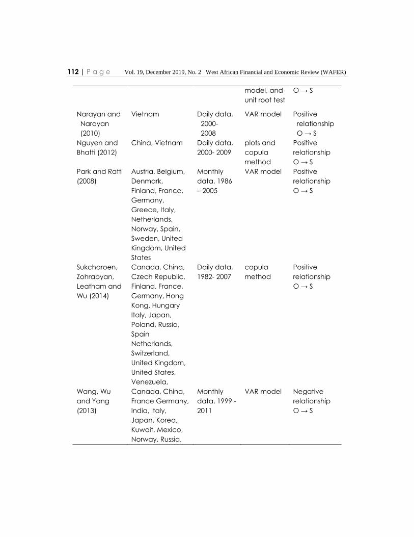
112 | P a g e Vol. 19, December 2019, No. 2 West African Financial and Economic Review (WAFER)
model, and
unit root test
O → S
Narayan and
Narayan
(2010)
Vietnam Daily data,
2000-
2008
VAR model Positive
relationship
O → S
Nguyen and
Bhatti (2012)
China, Vietnam Daily data,
2000- 2009
plots and
copula
method
Positive
relationship
O → S
Park and Ratti
(2008)
Austria, Belgium,
Denmark,
Finland, France,
Germany,
Greece, Italy,
Netherlands,
Norway, Spain,
Sweden, United
Kingdom, United
States
Monthly
data, 1986
– 2005
VAR model Positive
relationship
O → S
Sukcharoen,
Zohrabyan,
Leatham and
Wu (2014)
Canada, China,
Czech Republic,
Finland, France,
Germany, Hong
Kong, Hungary
Italy, Japan,
Poland, Russia,
Spain
Netherlands,
Switzerland,
United Kingdom,
United States,
Venezuela,
Daily data,
1982- 2007
copula
method
Positive
relationship
O → S
Wang, Wu
and Yang
(2013)
Canada, China,
France Germany,
India, Italy,
Japan, Korea,
Kuwait, Mexico,
Norway, Russia,
Monthly
data, 1999 -
2011
VAR model Negative
relationship
O → S
Moses K. Tule, J.S. Akuns, L.R. Balakeffi, , C.C. Chiemeke,S.A, Abdulsalam P a g e | 113
Saudi Arabia,
United Kingdom,
United States,
Venezuela
Others
Killian and
Park (2009)
United States Daily data VAR
framework
Oil demand
shocks do
depress stock
prices while
the oil supply
shock has
less impact.
Apergis and
Miller (2009)
Eight developed
countries
structural
VAR
The effect of
oil market
shocks is mild
and less
significant on
the stock
market for
countries
Notes: (1) → unidirectional, ↔ bidirectional. (2)S represents the stock market, and O
represents oil price.
3.0 Methodology
3.1 Modelling Framework
We consider the returns of the two variables of interest, namely oil price and stock
market price index, calculated here by taking the first difference of the natural
logarithm of the level series:
100* log(stock price)sr (1)
100* log( )or oil price (2)
Here, or are the returns on oil prices, sr are the returns on stock prices and is a first
difference operator.

114 | P a g e Vol. 19, December 2019, No. 2 West African Financial and Economic Review (WAFER)
3.1.1 Model Specification: Estimating Spillover Effects
Fundamentally, several models have been developed in the literature to deal with
spillover analyses. A key aspect of the study is to examine if volatility in oil prices is
transmitted into stock price volatility (is to investigate whether shocks in oil prices
transmitted to stock returns or have a spillover effect on the stock market).
Accordingly, the CCC model of Bollerslev (1990) and VAR-GARCH model of Ling and
McAleer (2003) is presented in this section. Constant conditional correlations were
assumed in the models, and it is not affected by the curse dimensionality when
compared with the VECH and BEKK models (read McAleer et al., 2008 and Caporin
and McAleer, 2009 for more details).
The Bollerslev (1990) CCC-MGARCH model is given below:
Conditional Mean equation: ; 1Y E Y Ft t t t (3)
t t tD
Conditional Variance equation: 1Var F H D D D Dt t t t t t t t t (4)
Where:
, ,1y y yt t mt is a vector of series under consideration; 1, ,i m
defines the
individual series in the model; m is the number of series being examined; 1, ,t n
represents the period covered by the series; n is the total number of observations;
1 , ,t t mt is a series of independently and identically distributed disturbances
for the individual series; tF denotes previous information available at time t ;
1 2 1 2, ,
1D diag h ht mtt
and the elements denote conditional standard deviations
for the respective series 1, , m . In other words, ,i th represents the conditional
variance for series i .
The Conditional Mean equations for the two-return series are given below:
Mean equation for stock price return: tsto
rsts
rssts
r,1,1,,
(5)
Mean equation for Oil price return: tots
roto
rooto
r,1,1,,
(6)

Moses K. Tule, J.S. Akuns, L.R. Balakeffi, , C.C. Chiemeke,S.A, Abdulsalam P a g e | 115
The Variance Equations for VAR-CCC-MGARCH (1, 1) are written as:
The Variance Equations for stock price returns:
121211112
12122
111111
th
th
ttc
th (7)
The Variance Equations for oil price returns:
122211212
12222
112122
th
th
ttc
th (8)
This implies that the conditional variance of each series, ,i th , 1, ,i m , indicates a
univariate GARCH process, given as:
2 2, ,,
1 1
;p q
i t i ir i t rik i t kk r
h h
(9)
where 1, ,k p ; 1, ,r q ; 1
p
ik
k
denotes the short run persistence or ARCH effect,
of shocks to series i , and
1 1
p q
ik irk r
denotes the long run persistence of shocks
to series i . The conditional covariance between the stock and oil market returns can
be expressed as:
sot so so oth h h (10)
The constant conditional correlation is represented byso
. The fundamental
underlying assumption for the implementation of the CCC-MGARCH model is that the
conditional correlation is constant over time. This is a very restrictive assumption, and
therefore, a formal pre-test must be carried out to verify if this assumption is valid or
not. The Engle-Sheppard (2001) CCC test that is chi-square distributed is considered in
this regard. This pre-test essentially tests the null hypothesis of constant correlation
against the alternative of dynamic conditional correlation (DCC). If the null hypothesis
of the Engle-Sheppard (2001) CCC test is not rejected; then, the CCC-MGARCH model
is appropriate; otherwise, it is not. More importantly, the CCC-MGARCH model also
assumes that negative and positive shocks of equal magnitude have same impacts
on the conditional variance. To isolate the asymmetric impacts of positive and
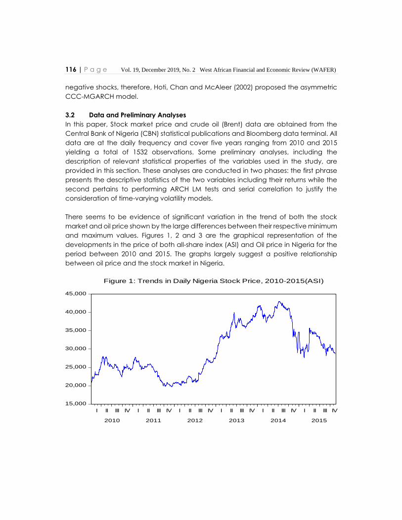
116 | P a g e Vol. 19, December 2019, No. 2 West African Financial and Economic Review (WAFER)
negative shocks, therefore, Hoti, Chan and McAleer (2002) proposed the asymmetric
CCC-MGARCH model.
3.2 Data and Preliminary Analyses
In this paper, Stock market price and crude oil (Brent) data are obtained from the
Central Bank of Nigeria (CBN) statistical publications and Bloomberg data terminal. All
data are at the daily frequency and cover five years ranging from 2010 and 2015
yielding a total of 1532 observations. Some preliminary analyses, including the
description of relevant statistical properties of the variables used in the study, are
provided in this section. These analyses are conducted in two phases: the first phrase
presents the descriptive statistics of the two variables including their returns while the
second pertains to performing ARCH LM tests and serial correlation to justify the
consideration of time-varying volatility models.
There seems to be evidence of significant variation in the trend of both the stock
market and oil price shown by the large differences between their respective minimum
and maximum values. Figures 1, 2 and 3 are the graphical representation of the
developments in the price of both all-share index (ASI) and Oil price in Nigeria for the
period between 2010 and 2015. The graphs largely suggest a positive relationship
between oil price and the stock market in Nigeria.
15,000
20,000
25,000
30,000
35,000
40,000
45,000
I II III IV I II III IV I II III IV I II III IV I II III IV I II III IV
2010 2011 2012 2013 2014 2015
Figure 1: Trends in Daily Nigeria Stock Price, 2010-2015(ASI)
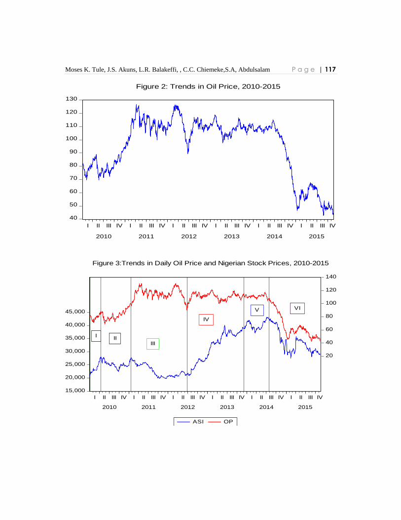
Moses K. Tule, J.S. Akuns, L.R. Balakeffi, , C.C. Chiemeke,S.A, Abdulsalam P a g e | 117
40
50
60
70
80
90
100
110
120
130
I II III IV I II III IV I II III IV I II III IV I II III IV I II III IV
2010 2011 2012 2013 2014 2015
Figure 2: Trends in Oil Price, 2010-2015
15,000
20,000
25,000
30,000
35,000
40,000
45,000
20
40
60
80
100
120
140
I II III IV I II III IV I II III IV I II III IV I II III IV I II III IV
2010 2011 2012 2013 2014 2015
ASI OP
III
III
IV
V VI
Figure 3:Trends in Daily Oil Price and Nigerian Stock Prices, 2010-2015

118 | P a g e Vol. 19, December 2019, No. 2 West African Financial and Economic Review (WAFER)
-6
-4
-2
0
2
4
6
8
10
I II III IV I II III IV I II III IV I II III IV I II III IV I II III IV
2010 2011 2012 2013 2014 2015
Figure 4: Daily Returns on Nigerian Stock Prices, 2010-2015
-10.0
-7.5
-5.0
-2.5
0.0
2.5
5.0
7.5
10.0
I II III IV I II III IV I II III IV I II III IV I II III IV I II III IV
2010 2011 2012 2013 2014 2015
Figure 5: Daily Oil Price Returns , 2010=2015

Moses K. Tule, J.S. Akuns, L.R. Balakeffi, , C.C. Chiemeke,S.A, Abdulsalam P a g e | 119
-10.0
-7.5
-5.0
-2.5
0.0
2.5
5.0
7.5
10.0
I II III IV I II III IV I II III IV I II III IV I II III IV I II III IV
2010 2011 2012 2013 2014 2015
RSTASI ROP
Figure 6: Daily Returns on Oil Price and Nigerian Stock Prices,2010-2015
Similar evidence of significant variation in the trend of both the stock market and oil
price is also observed for South Africa over the period 2010 and 2015. Like Nigeria, the
graphical representation also suggests a positive relationship between oil price and
the stock market in South Africa (see Figure 7). Figure 8 also illustrates the level of
volatility on the returns in the stock market in the presence of oil price shocks. The higher
the volatility clustering displayed in both markets reflects, the higher the standard
deviation obtained for the oil price series.

120 | P a g e Vol. 19, December 2019, No. 2 West African Financial and Economic Review (WAFER)
20,000
30,000
40,000
50,000
60,000
40
60
80
100
120
140
I II III IV I II III IV I II III IV I II III IV I II III IV I II III IV
2010 2011 2012 2013 2014 2015
jburg_Stock_Prices Oil_Prices
I
II
III
IVV
VI
VII
Figure 7: Trends in Daily Oil Price and South African Stock Prices, 2010-2015
We further consider relevant descriptive statistics and formal pre-tests in order to
evaluate the statistical properties of the series we are dealing with. Table 1 provides all
the relevant preliminary analyses for the return series.
The descriptive statistics for the returns cover the mean, standard deviation as well as
the distribution properties on the basis of skewness and kurtosis. The mean values
reported in the summary statistics indicate positive average returns in the stock market
for the period under consideration.
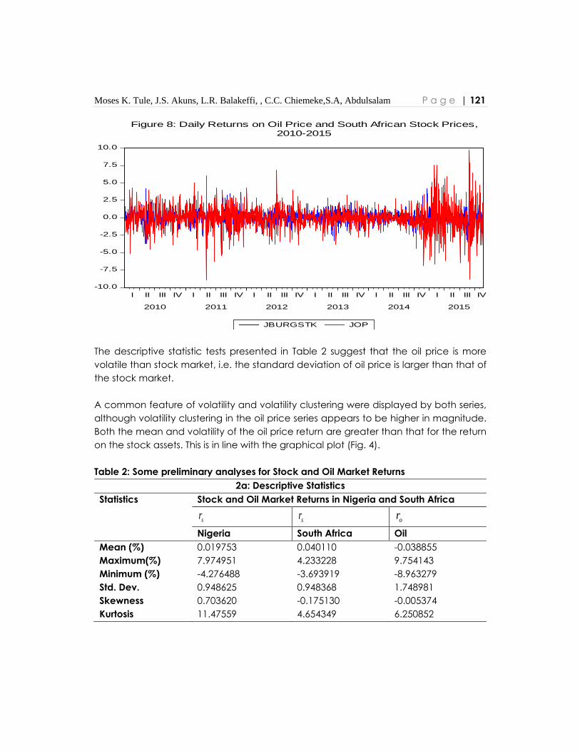
Moses K. Tule, J.S. Akuns, L.R. Balakeffi, , C.C. Chiemeke,S.A, Abdulsalam P a g e | 121
-10.0
-7.5
-5.0
-2.5
0.0
2.5
5.0
7.5
10.0
I II III IV I II III IV I II III IV I II III IV I II III IV I II III IV
2010 2011 2012 2013 2014 2015
JBURGSTK JOP
Figure 8: Daily Returns on Oil Price and South African Stock Prices,2010-2015
The descriptive statistic tests presented in Table 2 suggest that the oil price is more
volatile than stock market, i.e. the standard deviation of oil price is larger than that of
the stock market.
A common feature of volatility and volatility clustering were displayed by both series,
although volatility clustering in the oil price series appears to be higher in magnitude.
Both the mean and volatility of the oil price return are greater than that for the return
on the stock assets. This is in line with the graphical plot (Fig. 4).
Table 2: Some preliminary analyses for Stock and Oil Market Returns
2a: Descriptive Statistics
Statistics Stock and Oil Market Returns in Nigeria and South Africa
sr sr or
Nigeria South Africa Oil
Mean (%) 0.019753 0.040110 -0.038855
Maximum(%) 7.974951 4.233228 9.754143
Minimum (%) -4.276488 -3.693919 -8.963279
Std. Dev. 0.948625 0.948368 1.748981
Skewness 0.703620 -0.175130 -0.005374
Kurtosis 11.47559 4.654349 6.250852

122 | P a g e Vol. 19, December 2019, No. 2 West African Financial and Economic Review (WAFER)
2b: Conditional Heteroscedasticity and Autocorrelation Tests
ARCH LM (5) 6.82386 (0.00) 18.6007(0.00) 40.3931(0.00)
ARCH LM (10) 3.96024 (0.00) 15.0146 (0.00) 23.4031(0.00)
LB(5) 0.9096 (0.97) 7.7924 (0.168) 4.8778 (0.431)
LB(10) 2.3525 (0.99) 15.235 (0.124) 12.693 (0.241)
LB2(5) 40.805 (0.00) 132.66 (0.00) 303.05 (0.00)
LB2(10) 54.219 (0.00) 264.53 (0.00) 442.81 (0.00)
2c: Asymmetry test and CCC test
Stock_Price Stock Price Oil_Price
Nigeria South Africa Oil
Sign bias test 0.315(0.7527) 0.693 (0.44885) 2.769 (0.0057)
Negative size bias test 0.601 (0.5479) 1.110 (0.2672) 0.388 (0.6980)
Positive size bias test 0.610(0.5420) 2.978 (0.00295) 1.672 (0.0948)
Joint bias test 0.935(0.8170) 28.998 (0.0000) 11.916 (0.0077)
Engle-Sheppard CCC
2
2 test*
0.686 (0.710) 5.360 (0.0686)
Observations 1533 1533 1533
Note: The ARCH LM tests are related to the Engle (1982) test for conditional
heteroscedasticity. The LB and LB2denote the Ljung-Box tests for autocorrelations
comprising the standardised residuals in levels and squared standardised residuals,
respectively. The null hypothesis for the ARCH-LM test is stated as no ARCH effects in
the series (that is, it is not volatile) while the null hypothesis for LB test is stated as “there
is no series serially correlation on the series” or the series is not serially corrected. The
figures in parentheses represent the actual probability values. *2
2 Number of series
and degree of freedom
Table 2 presents some statistics on the autocorrelation function of the two series. We
presented both the Ljung–Box Q-statistic and Q2-statistic which tests for the null
hypothesis that there is no autocorrelation at lags 5 and 10. For both the stock price
and oil price return series, the null of no autocorrelation was rejected at the 1% level
judging by the Ljung–Box Q2-statistic. There seems, therefore, to be evidence of
autocorrelation in the two stock market series (see Table 2b).
Also, the ARCH-LM test indicates that all the series exhibit non-constant variance. In
other words, both oil price and stock market returns exhibit conditional
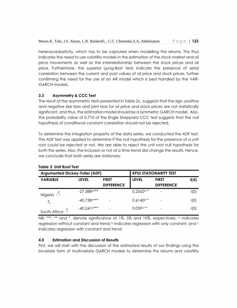
Moses K. Tule, J.S. Akuns, L.R. Balakeffi, , C.C. Chiemeke,S.A, Abdulsalam P a g e | 123
heteroscedasticity, which has to be captured when modelling the returns. This thus
indicates the need to use volatility models in the estimation of the stock market and oil
price movements as well as the interrelationship between the stock prices and oil
price. Furthermore, the superior Ljung-Box2 tests indicate the presence of serial
correlation between the current and past values of oil price and stock prices, further
confirming the need for the use of an AR model which is best handled by the VAR-
GARCH models.
3.3 Asymmetry & CCC Test
The result of the asymmetric tests presented in Table 2c, suggests that the sign, positive
and negative size bias and joint bias for oil price and stock prices are not statistically
significant, and thus, the estimation model should be a symmetric GARCH model. Also,
the probability value of 0.710 of the Engle Sheppard CCC test suggests that the null
hypothesis of conditional constant correlation should not be rejected.
To determine the integration property of the data series, we conducted the ADF test.
The ADF test was applied to determine if the null hypothesis for the presence of a unit
root could be rejected or not. We are able to reject the unit root null hypothesis for
both the series. Also, the inclusion or not of a time trend did change the results. Hence,
we conclude that both series are stationary.
Table 3: Unit Root Test
Argumented Dickey-Fuller (ADF) KPSS STATIONARITY TEST
VARIABLE LEVEL FIRST
DIFFERENCE
LEVEL FIRST
DIFFERENCE
I(d)
Nigeria - sr -27.588b*** - 0.2562b*** - I(0)
or -40.738b*** - 0.6140b*** - I(0)
South Africa - sr -40.241b*** - 0.039 b*** - I(0)
NB: ***, ** and *, denote significance at 1%, 5% and 10%, respectively. a indicates
regression without constant and trend; b indicates regression with only constant; and c
indicates regression with constant and trend
4.0 Estimation and Discussion of Results
First, we will start with the discussion of the estimated results of our findings using the
bivariate form of multivariate GARCH models to determine the returns and volatility
124 | P a g e Vol. 19, December 2019, No. 2 West African Financial and Economic Review (WAFER)
transmission between oil and stock markets in both the Nigerian and South African
stock markets. Specifically, the empirical framework was designed within the VAR (1)–
GARCH (1,1) model. Also, the estimated results relating to the optimal weights and
hedge ratios for the choice of holding oil -stock in a portfolio will then form the later
part of our discussion in this session.
The estimated results from the VAR(1)–GARCH(1,1) are presented in Table 4 for both
the oil-stock markets for Nigeria and South Africa. First, we observed from the
diagnostics that there are no remaining ARCH effects in the return series of stock, but
not for oil price for Nigeria after the estimation of the VAR(1)–GARCH(1,1). Similar results
of no ARCH effects could also be obtained in the return series for the stock market, but
not for the oil market in the case of South Africa. The McLeod-Li test at different lag
orders is used to test for the presence of ARCH effects. In the case of Ljung-Box tests,
there is no evidence of serial correlation at different lags for the two-return series in
both Nigeria and South Africa. Also, we observed significant explanatory power in the
stock market returns for the South African stock market more than in the Nigeria stock
market at their current values.
Return spillover between the two markets in both countries is assumed symmetric; that
is, positive and negative returns are assumed to have identical impacts. The
parameters of interest here are s [return spillover from stock price to oil price] and
o [return spillover from oil price to stock prices]. Nonetheless, we include own lagged
returns [ s and o ] in the conditional mean equations to ensure that spillover effects
are not confounded with serial dependence. As observed in Table 4, the return
spillover from stock price to oil price estimates are not statistically significant, indicating
that the returns in the oil market are not significantly influenced by the returns in the
stock market. However, the outcomes from oil price to stock price are statistically
significant, indicating that the returns in the stock market are influenced by the returns
in the oil market. However, investors in the stock market seem to take into account
the immediate past returns of changes in the stock market when making investment
decisions.
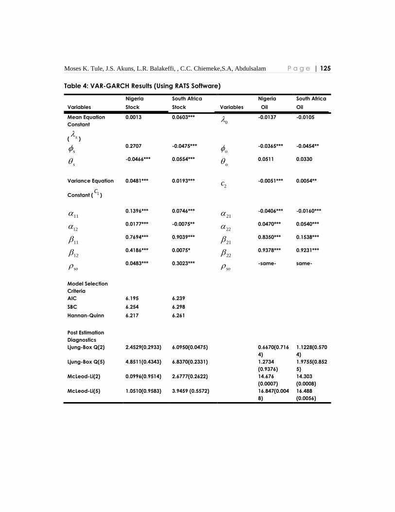
Moses K. Tule, J.S. Akuns, L.R. Balakeffi, , C.C. Chiemeke,S.A, Abdulsalam P a g e | 125
Table 4: VAR-GARCH Results (Using RATS Software)
Nigeria South Africa Nigeria South Africa
Variables Stock Stock Variables Oil Oil
Mean Equation
Constant
( s )
0.0013 0.0603*** 0
-0.0137 -0.0105
s
0.2707 -0.0475*** o
-0.0365*** -0.0454**
s
-0.0466*** 0.0554*** o
0.0511 0.0330
Variance Equation
Constant ( 1c )
0.0481*** 0.0193*** 2c
-0.0051*** 0.0054**
11
0.1396*** 0.0746*** 21
-0.0406*** -0.0160***
12
0.0177*** -0.0075** 22
0.0470*** 0.0540***
11
0.7694*** 0.9039*** 21
0.8350*** 0.1538***
12
0.4186*** 0.0075* 22
0.9378*** 0.9231***
so
0.0483*** 0.3023*** so
-same- same-
Model Selection
Criteria
AIC 6.195 6.239
SBC 6.254 6.298
Hannan-Quinn 6.217 6.261
Post Estimation
Diagnostics
Ljung-Box Q(2) 2.4529(0.2933) 6.0950(0.0475) 0.6670(0.716
4)
1.1228(0.570
4)
Ljung-Box Q(5) 4.8511(0.4343) 6.8370(0.2331) 1.2734
(0.9376)
1.9755(0.852
5)
McLeod-Li(2) 0.0996(0.9514) 2.6777(0.2622) 14.676
(0.0007)
14.303
(0.0008)
McLeod-Li(5) 1.0510(0.9583) 3.9459 (0.5572) 16.847(0.004
8)
16.488
(0.0056)

126 | P a g e Vol. 19, December 2019, No. 2 West African Financial and Economic Review (WAFER)
The optimal lag order for the VAR model is selected using the AIC and SIC information
criteria; Note: ***, ** and *denote statistical significance at 1%, 5% and 10% levels.
Figures in parentheses represent p-values.
The estimates of the one-period lagged own stock returns are positive for Nigeria, but
negative in the case of South Africa and both stock market returns are statistically
significant. This result also indicates the interdependence of returns of the two markets.
On the other hand, a negative and statistically significant one period lagged of oil
price returns was obtained in the estimates in the case of South Africa, while, in the
case Nigeria, it was negetive and statistically insignificant. Evidently, a much higher
elasticity of the stock market’s reactions to oil price change was obtained in this regard
at an estimated coefficient of 0.27. The presence of negative shock spillover from oil
to stock in South Africa is not unconnected with less reliance on the stock market on
oil companies, but on gold companies, financial and service-oriented companies.
These features are likely to undermine market operations on investment and
speculations. Generally, shock transmission through previous oil price changes tend to
have a positive and significant effect on stock markets in Nigeria, but a negative and
significant effect in the case of the South Africa’s stock market. The level of impact
tends, therefore, to be minimal in South Africa’s stock market when compared with
the Nigerian stock market. It is expected that these results will assist investors to better
understand the dynamics in both markets in these countries and be able to forecast
future returns on stocks.
Regarding the conditional volatility equations, the volatilities of stock and oil returns
are sensitive to both own past shocks as well as past own conditional variance. The
estimated results show that both ARCH and GARCH coefficients are significant in most
cases. The magnitude of the reactions or interactions of GARCH-term past own
conditional volatility seems to be quite significant in both countries. In this regard, we
observed that the coefficients of the ARCH-terms, which measure the effect of past
shocks on conditional volatility is rather very small and quite reflected in a sluggish
change in the general conditional volatility. Also, the relatively sizable GARCH-term
estimates, which measure the impact of past volatility on current volatility, are quite
significant in both countries and display a steady variation of conditional volatility over
time.
In terms of volatility spillovers from oil to stock markets in both countries, the estimated
coefficients are much smaller, and thus, the impacts of past shocks and past volatility
of oil returns on the volatility of stock markets are quite minimal.
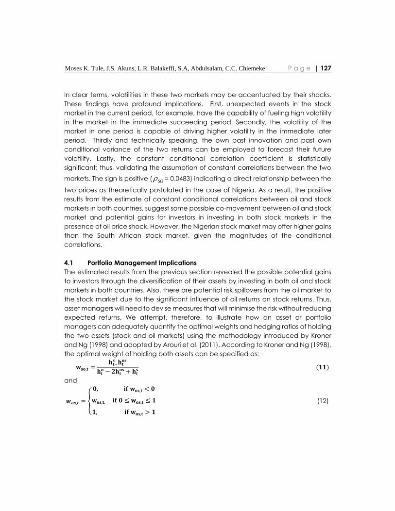
Moses K. Tule, J.S. Akuns, L.R. Balakeffi, S.A, Abdulsalam, C.C. Chiemeke P a g e | 127
In clear terms, volatilities in these two markets may be accentuated by their shocks.
These findings have profound implications. First, unexpected events in the stock
market in the current period, for example, have the capability of fueling high volatility
in the market in the immediate succeeding period. Secondly, the volatility of the
market in one period is capable of driving higher volatility in the immediate later
period. Thirdly and technically speaking, the own past innovation and past own
conditional variance of the two returns can be employed to forecast their future
volatility. Lastly, the constant conditional correlation coefficient is statistically
significant; thus, validating the assumption of constant correlations between the two
markets. The sign is positive ( SO = 0.0483) indicating a direct relationship between the
two prices as theoretically postulated in the case of Nigeria. As a result, the positive
results from the estimate of constant conditional correlations between oil and stock
markets in both countries, suggest some possible co-movement between oil and stock
market and potential gains for investors in investing in both stock markets in the
presence of oil price shock. However, the Nigerian stock market may offer higher gains
than the South African stock market, given the magnitudes of the conditional
correlations.
4.1 Portfolio Management Implications
The estimated results from the previous section revealed the possible potential gains
to investors through the diversification of their assets by investing in both oil and stock
markets in both countries. Also, there are potential risk spillovers from the oil market to
the stock market due to the significant influence of oil returns on stock returns. Thus,
asset managers will need to devise measures that will minimise the risk without reducing
expected returns. We attempt, therefore, to illustrate how an asset or portfolio
managers can adequately quantify the optimal weights and hedging ratios of holding
the two assets (stock and oil markets) using the methodology introduced by Kroner
and Ng (1998) and adopted by Arouri et al. (2011). According to Kroner and Ng (1998),
the optimal weight of holding both assets can be specified as:
𝐰𝐬𝐨,𝐭 =𝐡𝐭−
𝐬 𝐡𝐭𝐨𝐬
𝐡𝐭𝐨 − 𝟐𝐡𝐭
𝐨𝐬 + 𝐡𝐭𝐬 (𝟏𝟏)
and
𝒘𝒐𝒔,𝒕 = {
𝟎, 𝐢𝐟 𝐰𝐨𝐬,𝐭 < 𝟎
𝐰𝐨𝐬,𝐭, 𝐢𝐟 𝟎 ≤ 𝐰𝐨𝐬,𝐭 ≤ 𝟏
𝟏, 𝐢𝐟 𝐰𝐨𝐬,𝐭 > 𝟏
(12)

128 | P a g e Vol. 19, December 2019, No. 2 West African Financial and Economic Review (WAFER)
Where 𝑤𝑠𝑜,𝑡 represents the weight of oil in a one dollar consisting of two assets within a
portfolio at time t: and ℎ𝑡𝑜𝑠 refers to the conditional covariance between oil and stock
market returns at time t. This means that the optimal weight of the stock market index
within the portfolio under consideration is 1 − 𝑤𝑠𝑜,𝑡.
Table 5 reports the values of 𝑤𝑠𝑜,𝑡 (optimal weights) for the two countries. They vary
from 7.28 per cent for Nigeria to 4.78 per cent for South Africa. This implies that the
optimal weight of holding of oil in a one-dollar oil-stock market portfolio would be 7.28
per cent in the case of Nigeria and the remaining budget of 92.72 per cent should be
invested in the stock market. In the case of South Africa, optimal the holding of oil is as
low as 4.78 per cent, while the rest of 95.22 is invested in stock market. This overall result
suggests that investors should acquire more stocks than oil in their portfolio in both
countries to curtail the risk without reducing the expected returns is not surprising. The
stock markets in South Africa depend less on oil companies, but more on gold
companies, financial and service oriented companies.
Regarding the hedge ratios, we also applied the methodology introduced by Kroner
and Sultan (1993) and adopted by Arouri et al. (2011) to examine a portfolio of two
assets that include oil and stock market index. Evidently, the likely risk of this portfolio
will be negligible if a short position of one dollar in the oil market can be hedged by a
long position of 𝜌𝑡 dollars in the stock market index, and it is specified as:
𝜌𝑜𝑠,𝑡 =ℎ𝑡
𝑜𝑠
ℎ𝑡𝑠 (13)
Table 5: Optimal Portfolio weights and Hedge ratios (With Brent oil prices)
Nigeria South Africa
,so t 0.07278 0.04778
,so t 0.15926 0.73803
Moses K. Tule, J.S. Akuns, L.R. Balakeffi, S.A, Abdulsalam, C.C. Chiemeke P a g e | 129
Table 5 presents the values of the hedge ratios computed for both countries using
equation (11). We observed that the hedging ratios are quite high in South Africa when
compared to that of Nigeria. The ratios range from 73.80 per cent in South Africa to
15.93 per cent in Nigeria. The observed higher values obtained for the hedge ratios in
both countries suggest that hedging effectiveness relating to both stock and oil
markets in both countries will not deliver the desired outcome to investors.
The results obtained above implies that of one dollar short position in the oil market
should be longed by 73.80 and 15.93 per cent in both countries.
4.2 Evaluation for Robustness
To further evaluate the robustness of the regression results obtained in the case of the
optimal weights and hedging ratios for both countries, we replaced the Brent oil price
with WTI oil price. As you will recall, the oil price was measured using Brent oil price as
oil price proxy. In this regard, we re-estimated all the equations using WTI oil price as oil
price proxy. The results, as shown in table 6, indicate that our analyses are robust to
different oil price proxies. This implies that using different oil price proxies to determine
an optimal portfolio and hedging ratios for both countries will produce similar
inferences for both short and long-run relationships.
Table 6: Optimal Portfolio weights and Hedge Ratios Robustness Check (With WTI Oil
prices)
5.0 Summary and Conclusion
This paper investigates Volatility spillovers between oil and stock markets: Evidence
from Nigeria and South Africa using daily returns from January 2010 to December 2015.
The bivariate form of the VAR–CCC-GARCH(1,1) model introduced by Ling and
McAleer (2003) was adopted. We also examined the optimal weights and hedge
ratios for the choice of holding oil -stock in a portfolio. The overall results indicate the
presence of return and volatility spillovers from oil to stock market in both countries. In
essence, own-shocks to stock price and oil price increase the level of volatility of their
respective markets. However, when there is a shock to one market, it tends to reduce
the risk-adjusted returns of the other market. Also, our findings also suggest that adding
oil to a well-diversified portfolio of stocks issued in both countries will not lead to an
improvement in the overall risk-adjusted return and oil price risk cannot be hedged
effectively in both countries. Our results tend to vary across countries and in the period
considered. This outcome seems to support outcomes from other studies.

130 | P a g e Vol. 19, December 2019, No. 2 West African Financial and Economic Review (WAFER)
However, the outcomes from oil price to stock price are statistically significant,
indicating that the returns in the stock market are influenced by the returns in the oil
market. However, investors in the stock market seem to take into account the
immediate past returns of changes in the stock market when making investment
decisions. The estimates of the one-period lagged own returns for the two series are
positive, but only stock market is statistically significant.
Also, the volatilities of stock and oil returns are sensitive to both own past shocks as well
as past own conditional variance. In clear terms, volatilities in these two markets may
be accentuated by their own shocks. These findings have profound implications. First,
unexpected events in the stock market in the current period, for example, have the
capability of fueling high volatility in the market in the immediate succeeding period.
Secondly, the volatility of the market in one period are capable of driving higher
volatility in the immediate later period. Thirdly and technically speaking, the own past
innovation and past own conditional variance of the two returns can be employed to
forecast their future volatility. Lastly, the constant conditional correlation coefficient is
statistically significant; thus, validating the assumption of constant correlations
between the two markets. The sign is positive ( SO = 0.048) indicating a direct
relationship between the two prices as theoretically postulated.
Moses K. Tule, J.S. Akuns, L.R. Balakeffi, S.A, Abdulsalam, C.C. Chiemeke P a g e | 131
Reference
Abdelaziz M, Chortareas G, & Upollinni A 2008. Stock Price, Exchange Rates and Oil:
Evidence from Middle-EastbOil Exporting Countries- Unpublished
Manuscript.From http://www.iiste.org/journals/index.php/EJBMb(Retrieved
April 18, 2010).
Adebiyi, M. A., Adenuga, A. O., Abeng, M. O., & Omanukwue, P. N. (2009, June). Oil
price shocks, exchange rate and stock market behaviour: Empirical evidence
from Nigeria. In Proceedings of the 14th Annual Conference of the African
Econometric Society.
Adetunji Babatunde, Adenikinju, O. and Adenikinju, A. F. (2013). Oil price shocks and
stock market behaviour in Nigeria. Journal of Economic Studies, 40(2), 180-202.
Arouri, M. E. H., Lahiani, A., & Bellalah, M. (2010). Oil price shocks and stock market
returns in oil-exporting countries: The case of GCC countries. International
Journal of Economics and Finance, 2(5), 132.
Arouri, Mohamed El Hedi, Amine L., and Duc K. N. (2011):. "Return and volatility
transmission between world oil prices and stock markets of the GCC countries."
Economic Modelling 28.4,1815-1825.
Arouri, M. E. H., Jouini, J., & Nguyen, D. K. (2011). Volatility spillovers between oil prices
and stock sector returns: Implications for portfolio management. Journal of
International money and finance, 30(7), 1387-1405.
Apergis, N and Miller, M.S (2008): “Do Structural Oil-Market Shocks Affect Stock Prices?”
Economics Working Papers, Department of Economics, University of
Connecticut, USA
Apergis, N., & Miller, S. M. (2009). Do structural oil-market shocks affect stock prices?.
Energy Economics, 31(4), 569-575.
Awartani, B., & Maghyereh, A. I. (2013). Dynamic spillovers between oil and stock
markets in the Gulf Cooperation Council Countries. Energy Economics, 36, 28-
42.
Basher, S. A., & Sadorsky, P. (2006). Oil price risk and emerging stock markets. Global
Finance Journal, 17(2), 224-251.
Basher, S. A., Haug, A. A., & Sadorsky, P. (2012). Oil prices, exchange rates and
emerging stock markets. Energy Economics, 34(1), 227-240.
Bollerslev, T. (1990). Modelling the coherence in short-run nominal exchange rates: a
multivariate generalized ARCH model. The review of economics and statistics,
498-505.
Boyer, M. M., & Filion, D. (2007). Common and fundamental factors in stock returns of
Canadian oil and gas companies. Energy Economics, 29(3), 428-453.

132 | P a g e Vol. 19, December 2019, No. 2 West African Financial and Economic Review (WAFER)
Broadstock, D. C., & Filis, G. (2014). Oil price shocks and stock market returns: New
evidence from the United States and China. Journal of International Financial
Markets, Institutions and Money, 33, 417-433.
Caporin, M., & McAleer, M. (2012). Do we really need both BEKK and DCC? A tale of
two multivariate GARCH models. Journal of Economic Surveys, 26(4), 736-751.
Caporale, G. M., Ali, F. M., & Spagnolo, N. (2015). Oil price uncertainty and sectoral
stock returns in China: A time-varying approach. China Economic Review, 34,
311-321.
Cong, R. G., Wei, Y. M., Jiao, J. L., & Fan, Y. (2008). Relationships between oil price
shocks and stock market: An empirical analysis from China. Energy Policy, 36(9),
3544-3553.
Chang, C. L., McAleer, M., & Tansuchat, R. (2013). Conditional correlations and
volatility spillovers between crude oil and stock index returns. The North
American Journal of Economics and Finance, 25, 116-138.
Chiou, J. S., & Lee, Y. H. (2009). Jump dynamics and volatility: Oil and the stock markets.
Energy, 34(6), 788-796.
Cunado, J., & de Gracia, F. P. (2014). Oil price shocks and stock market returns:
Evidence for some European countries. Energy Economics, 42, 365-377.
Dagher, L., & El Hariri, S. (2013). The impact of global oil price shocks on the Lebanese
stock market. Energy, 63, 366-374.
El-Sharif, I., Brown, D., Burton, B., Nixon, B., & Russell, A. (2005). Evidence on the nature
and extent of the relationship between oil prices and equity values in the UK.
Energy Economics, 27(6), 819-830.
Eryiğit, M. (2009). Effects of Oil Price Changes on the Sector Indices of Istanbul Stock
Exchange‖. International Research Journal of Finance and Economics, 25(2),
209-216.
Faff, R. W., & Brailsford, T. J. (1999). Oil price risk and the Australian stock market. Journal
of Energy Finance & Development, 4(1), 69-87.
Ferson, W. E., & Harvey, C. R. (1994). Sources of risk and expected returns in global
equity markets. Journal of Banking & Finance, 18(4), 775-803.
Filis, G., Degiannakis, S., & Floros, C. (2011). Dynamic correlation between stock market
and oil prices: The case of oil-importing and oil-exporting countries.
International Review of Financial Analysis, 20(3), 152-164.
Gbadebo O.O. (2008) Crude Oil and the Nigerian Economic Performance: Oil and
Gas Business http://www.ogbus.ru/eng.
Gil-Alana, L. A., Shittu, O. I., & Yaya, O. S. (2014). On the persistence and volatility in
European, American and Asian stocks bull and bear markets. Journal of
International Money and Finance, 40, 149-162.
Moses K. Tule, J.S. Akuns, L.R. Balakeffi, S.A, Abdulsalam, C.C. Chiemeke P a g e | 133
Glosten, L. R., Jagannathan, R., & Runkle, D. E. (1993). On the relation between the
expected value and the volatility of the nominal excess return on stocks. The
journal of finance, 48(5), 1779-1801.
Hamilton, J. D. (1988). Rational-expectations econometric analysis of changes in
regime: An investigation of the term structure of interest rates. Journal of
Economic Dynamics and Control, 12(2-3), 385-423.
Hamilton, J. D. (1990). Analysis of time series subject to changes in regime. Journal of
econometrics, 45(1), 39-70.
Hammoudeh, S., & Li, H. (2004). The impact of the Asian crisis on the behavior of US
and international petroleum prices. Energy Economics, 26(1), 135-160.
Hammaoudeh, G and Li, (2004) “Risk-return Realtionships in oil-sensitive stock markets”,
Finance Letters, Vol. 2 No. 3, pp. 33-49
Hammoudeh, S., Dibooglu, S., & Aleisa, E. (2004). Relationships among US oil prices and
oil industry equity indices. International Review of Economics & Finance, 13(4),
427-453.
Hammoudeh, S. and Huimin, L. 2005, Oil sensitivity and systematic risk in oil-sensitive
stock indices, Journal of Economics and Business, 57, 1-21.
He, Y., Wang, S., & Lai, K. K. (2010). Global economic activity and crude oil prices: A
cointegration analysis. Energy Economics, 32(4), 868-876.
Hoti, S., Chan, F., & McAleer, M. (2002, July). Structure and asymptotic theory for
multivariate asymmetric volatility: Empirical evidence for country risk ratings. In
Australasian Meeting of the Econometric Society, Brisbane, Australia (p. 2002).
Huang, R. D., & Stoll, H. R. (1996). Dealer versus auction markets: A paired comparison
of execution costs on NASDAQ and the NYSE. Journal of Financial Economics,
41(3), 313-357.
Huang R.D, Masulis RW, Stoll HR (1996) “Energy shocks and financial markets” Journal
of Future Markets, 16: 1- 27.
Jones, C. M., & Kaul, G. (1996). Oil and the stock markets. The Journal of Finance, 51(2),
463-491.
Kang, W., Ratti, R. A., & Yoon, K. H. (2015). The impact of oil price shocks on the stock
market return and volatility relationship. Journal of International Financial
Markets, Institutions and Money, 34, 41-54.
Kaneko, T., & Lee, B. S. (1995). Relative importance of economic factors in the US and
Japanese stock markets. Journal of the Japanese and International
Economies, 9(3), 290-307.
Kilian, L. (2014), “Oil Price Shocks: Causes and Consequences,” forthcoming: Annual
Review of Resource Economics.

134 | P a g e Vol. 19, December 2019, No. 2 West African Financial and Economic Review (WAFER)
Kilian, L., Park, C., 2009. The impact of oil price shocks on the U.S. stock market. Int.Econ.
Rev. 50, 1267–1287.
Kim, I. M., & Loungani, P. (1992). The role of energy in real business cycle models.
Journal of Monetary Economics, 29(2), 173-189.
Kling, J. L. (1985). Oil price shocks and stock market behaviour. The Journal of Portfolio
Management, 12(1), 34-39.
Kroner, K. F., & Sultan, J. (1993). Time-varying distributions and dynamic hedging with
foreign currency futures. Journal of financial and quantitative analysis, 28(04),
535-551.
Kroner, K. F., & Ng, V. K. (1998). Modelling asymmetric comovements of asset returns.
Review of Financial Studies, 11(4), 817-844.
Lin, B., Wesseh, P. K., & Appiah, M. O. (2014). Oil price fluctuation, volatility spillover and
the Ghanaian equity market: Implication for portfolio management and
hedging effectiveness. Energy Economics, 42, 172-182.
Ling, S., & McAleer, M. (2003). Asymptotic theory for a vector ARMA-GARCH model.
Econometric Theory, 19(02), 280-310.
Lin, B., Wesseh, P. K., & Appiah, M. O. (2014). Oil price fluctuation, volatility spillover and
the Ghanaian equity market: Implication for portfolio management and
hedging effectiveness. Energy Economics, 42, 172-182.
Louis, R. J., & Balli, F. (2014). Oil Price and Stock Market Synchronization in Gulf
Cooperation Council Countries. Emerging Markets Finance and Trade, 50(1),
22-51.
Masih, R., Peters, S., & De Mello, L. (2011). Oil price volatility and stock price fluctuations
in an emerging market: evidence from South Korea. Energy Economics, 33(5),
975-986.
McAleer, M., Chan, F., Hoti, S., and Lieberman, O (2008), Generalized autoregressive
conditional correlation, Econometric Theory, 24-6, 1554-1583
Miller, J. I., & Ratti, R. A. (2009). Crude oil and stock markets: Stability, instability, and
bubbles. Energy Economics, 31(4), 559-568.
Mensi, W., Beljid, M., Boubaker, A., & Managi, S. (2013). Correlations and volatility
spillovers across commodity and stock markets: Linking energies, food, and
gold. Economic Modelling, 32, 15-22.
Miller, J. I., & Ratti, R. A. (2009). Crude oil and stock markets: Stability, instability, and
bubbles. Energy Economics, 31(4), 559-568.
Moses K. Tule, Umar B. Ndako, Samuel F. Onipede (2017) Oil price shocks and volatility
spillovers in the Nigerian sovereign bond market, Review of Financial
Economics 35 (2017) 57–65
Moses K. Tule, J.S. Akuns, L.R. Balakeffi, S.A, Abdulsalam, C.C. Chiemeke P a g e | 135
Moses K. Tule, Mela Dogo, Godfrey Uzonwanne (2018), Volatility of stock market returns
and the naira exchange rate, Global Finance Journal, Volume 35, February
2018, Pages 97 – 105
Narayan, P. K., & Narayan, S. (2010). Modelling the impact of oil prices on Vietnam’s
stock prices. Applied Energy, 87(1), 356-361.
Nguyen, C. C., & Bhatti, M. I. (2012). Copula model dependency between oil prices
and stock markets: Evidence from China and Vietnam. Journal of International
Financial Markets, Institutions and Money, 22(4), 758-773.
Papapetrou, E. (2001). Oil price shocks, stock market, economic activity and
employment in Greece. Energy Economics, 23(5), 511-532.
Park, J., & Ratti, R. A. (2008). Oil price shocks and stock markets in the US and 13
European countries. Energy Economics, 30(5), 2587-2608.
Rasche, R. H., & Tatom, J. A. (1977). Energy resources and potential GNP. Federal
Reserve Bank of St. Louis Review, (Jun), 10-24.
Rasche, R. and J. Tatom (1981). “Energy Price Shocks, Aggregate Supply and Monetary
Policy: The Theory and the International Evidence”. Carnegie-Rochester
Conference Series on Public Policy 14 (0), 9 – 93.
Rotemberg, J. J., & Woodford, M. (1996). Imperfect competition and the effects of
energy price increases on economic activity (No. w5634). National Bureau of
Economic Research.
Sadorsky, P. (1999). Oil price shocks and stock market activity. Energy Economics, 21(5),
449-469.
Salisu, A. A., & Mobolaji, H. (2013). Modelling returns and volatility transmission between
oil price and US–Nigeria exchange rate. Energy Economics, 39, 169-176.
Salisu, A. A., Isah, K. O., Oyewole, O. J., & Akanni, L. O. (2017). Modelling oil price-
inflation nexus: The role of asymmetries. Energy, 125, 97-106.
Skintzi, V. D., & Refenes, A. P. N. (2005). Implied correlation index: A new measure of
diversification. Journal of Futures Markets, 25(2), 171-197.
Sukcharoen, K., Zohrabyan, T., Leatham, D., & Wu, X. (2014). Interdependence of oil
prices and stock market indices: A copula approach. Energy Economics, 44,
331-339.
Wang, Y., Wu, C., & Yang, L. (2013). Oil price shocks and stock market activities:
Evidence from oil-importing and oil-exporting countries. Journal of
Comparative Economics, 41(4), 1220-1239.
Zhang, C., & Chen, X. (2011). The impact of global oil price shocks on China’s stock
returns: Evidence from the ARJI (-ht)-EGARCH model. Energy, 36(11), 6627-6633.

136 | P a g e Vol. 19, December 2019, No. 2 West African Financial and Economic Review (WAFER)

P a g e | 137
OPTIMAL CAPITAL ACCUMULATION AND BALANCED GROWTH PATHS IN AN
EXOGENOUS GROWTH SETTING FOR NIGERIA (2017-2030): DGE FRAMEWORK
Ernest Simeon O. Odior*1
Abstract
This study uses the first key equations of the Ramsey–Cass–Koopmans and Solow
neoclassical growth models to empirically project the likely optimal growth path for
capital stock in Nigeria, if the models’ assumptions stay at expected. The study used
a Dynamic General Equilibrium (DGE) framework to estimate the optimal capital
accumulation and the balanced growth paths over a finite planning period 2017 to
2030. The results of dynamic macroeconomic model show that, the growth path of
capital stock is characterised by constant return to scale, decreasing discount factor
and increasing rate of savings. The results also show that, an increase in capital
accumulation also leads to an increase in income, implying that capital is at optimal
to predict a higher growth rate of income in the long-run. The Study concludes
with an overwhelming evidence that rapid and sustained capital and income growth
is critical to economic growth and the well-being of a nation. Therefore, it is important
to devise ways of promoting capitalist economic development. The study
recommends that technological and labour effectiveness should be the basis for
capital accumulation and balanced growth for the Nigerian economy.
Keywords: Capital Accumulation, Neoclassical Growth Models, Nigeria, DGE
JEL classification: E13, D50
1.0 Introduction
For many years, economists have dealt with questions regarding the growth path of
an economy, the optimal capital accumulation and how these parameters can be
influenced. Capital was important in the early ages of growth, but it would also be
erroneous to think that it has no special place in today’s seemingly-capitalized
economies. These developments notwithstanding, the core of the neoclassical growth
model remains its original setting (Mankiw, David &Weil, 1992).
*Corresponding author’s e-mail: [email protected];[email protected], Phone +23480-
62088200; +2347058074040 1Department of Economics, Faculty of Social Sciences, University of Lagos, Akoka, Lagos, Nigeria

P a g e | 138 Ernest Simeon O. Odior, PhD
The accumulation of capital goods represents foregone consumption, which
necessitates a reward to capital in the form of interest, rent, royalties or capital gains,
greater profits or social benefit derived. The rate of accumulation of an economy's
physical stock of capital is an important determinant of the rate of growth of an
economy and is represented in various production functions and economic growth
models. The process of adding to the net physical capital stock of an economy in an
attempt to achieve greater total output is term capital accumulation or the
accumulation of capital.
This above stated process is a problem in concave programming in linear spaces.
Hence, this study problem is formulating an optimal growth model for a developing
economy like Nigeria with a finite time horizon. The main objective of this study
therefore, is to use the first key equations of the Ramsey–Cass–Koopmans (RCK) and
Solow models to empirically project the optimal growth path for capital stock in the
long-run for the Nigerian economy or finding a growth path over which the criterion
function is maximized among all feasible growth paths, if all other things being equal.
Also, the study empirically determins if capital stock and income converge to their steady
state equilibrium on the balanced growth paths in the exogenous productivity growth
models. That is, whether capital is at optimal to predict a higher growth rate of
income in the long-run.
The first key equations of the RCK model is the state equation for capital accumulation,
while the Solow model is the model of capital steady state. This study window (2017 to
2030) has been shortened to 2030 agenda for sustainable development goals. The
research questions to analyse is as follows: what is the optimal path of traverse for a
developing economy, which has a certain capital stock embodying an old technique
(i.e. one with a lower labour productivity) and is saddled additionally with disguised
unemployment, if it is to be transformed into one where the entire labour force is
assumed to be growing at an exogenously given rate? Does the economy reach a
long run equilibrium with a constant growth rate, or does growth fizzle out in the long-
run?
Given the popularity the RCK and Solow growth models at large, surprisingly little
attention has been paid to mechanics of capital accumulation, possibly because of
difficulties involved in measurement of the capital stock. One notable exception is a
series of study investigating movements of the economy's capital-output ratio
(McQuinn & Whelan, 2007, Hall & Jones, 1997); yet, their analyses are based on the
speed of convergence equation, not the growth path of the capital-output ratio per
Vol. 19, December 2019, No. 2 West African Financial and Economic Review (WAFER) P a g e | 139
se. Also, there are limited studies on the quantitative analysis and derivation regarding
the optimal capital growth paths for the Nigerian economy.
The justification for this study is to add to the body of comparative evidence available
on the study of economic growth theories. Economic growth deals with increase in the
level of output and it is important to study and devise ways of increasing output. Most
growth theories or models equate output growth with the level of capital
accumulation. Studying these growth theories or models should not be end in
themselves, the application of these theories to the economies of the developing
nations like Nigeria, is most important.
Therefore, efforts should be made to increase capital stock in a poor nation like
Nigeria. This will help the nation to move to being self-sufficient in capital, that will lead
to output growth, if all other things being equal. The gap this study is likely to fill, is to
investigate empirically, the application of RCK and Solow growth models on the
Nigerian economy, using a dynamic nonlinear optimization approach. This paper
equally contributes to the literature on optimal capital growth and national income
growth.
The rest of the paper is organised as follows. Section 1 presents the introductory part of
the study, while 2 presents brief review of relevant literature. Section 3 is the sets of
theoretical framework of the study. Section 4 is the study methodology. Section 5 is the
analysis of simulation results, Section 6 is the study conclusion and section 7 is policy
implications of the study.
2.0 Review of Literature
In economic growth literature, one of the important contributions to modern growth
theory have been the works of Solow (1956) and Swan (1956). The fundamental
feature of the Solow-Swan neoclassical growth model, also known as the exogenous
growth model, is its special specification, according to which the neoclassical
production function makes the assumption of constant returns to scale, diminishing
returns to each input and some positive and smooth elasticity of substitution between
the inputs. The Solow-Swan production function is applied along with a constant-
saving-rate rule in order to generate a simple general equilibrium model of the
economy.
A key prediction of these neoclassical growth models which has been frequently
applied as an empirical hypothesis in recent years is conditional convergence, in the

P a g e | 140 Ernest Simeon O. Odior, PhD
sense that the lower the starting level of per capita GDP, compare to the long-run or
steady-state position, the faster the growth rate. This is due to the assumption of
diminishing returns to capital according to which economies that have less capital per
worker tend to have higher rates of return and higher growth rates. The convergence
is conditional in the Solow-Swan model, because the steady-state levels of capital and
output per worker depend on the saving rate, the growth rate of population and the
position of the production function that might vary across economies (Mansour &
Hosainpour, 2011),
Cass (1965) & Koopmans (1965) applied Ramsey’s analysis of consumer optimization
to the neoclassical growth model in order to make adequate preparation for an
endogenous determination of the saving rate. This extension tends to preserve the
hypothesis of conditional convergence, while allowing for strong transitional dynamics.
However, it is not easy to create compatibility between the theory of technological
change and the neoclassical framework; because the standard assumptions of
competition cannot be met since technological progress requires the creation of new
ideas which are partially non-rival.
Hall & Jones (1999) showed that differences in physical capital and human capital can
only partly explain the variation in output per worker. According to this research, a
large amount of variation in the level of the Solow residual can be found across
countries. The differences in capital accumulation, productivity and output per worker
are caused by differences in institutions and government policies, i.e., by social
infrastructure. Social infrastructure was treated as endogenous factor in this research.
Across 127 countries selected for this study, a powerful and close association was fund
between output per worker and measures of social infrastructure. Countries with long-
standing policies are in favour of productive activities, rather than diversion, in order to
produce much more output per worker. For example, their analysis suggested that the
observed difference in social infrastructure between Niger and the United States is
more than enough to explain the 35-fold difference in output per worker.
Using panel data analysis, Hoeffler (2000) addressed this question that whether Africa's
growth performance can be accounted in the framework of the augmented Solow
model. The findings of the research showed that if unobserved country specific effects
and the endogeneity of investment are taken, this model can account for Africa's low
growth performance. According to these findings, Africa’s low investment ratios and
high population growth rates are sufficient to explain Africa's low growth rates. Also,
Heston, Summers & Aten (2002) equally show that, the derived capital growth
Vol. 19, December 2019, No. 2 West African Financial and Economic Review (WAFER) P a g e | 141
equations are empirically testable, owing to the well-known reduced form equation to
measure the so-called conditional convergence. They show that the data on capital
stock of the economy are available. This means a potential for a new method to test
conditional convergence (Mankiw, David &Weil, 1992).
Rina & Wisch (2005) compare the optimal capital stock accumulation in a classical
Ramsey model with production shocks for a risk neutral expected utility maximizer and
a loss averse prospect theory maximizer. They show that in the expected utility case,
the capital stock is on average the same as in the deterministic Ramsey growth model.
However, with prospect theory, one can expect a capital stock which is higher than in
the deterministic Ramsey model and given certain assumptions even higher than
Solow’s golden-rule capital stock.
Pritchett (2006) showed that, in spite of much progress in the growth literature, there
are still a considerable gap between the logic of academic interests and the needs
of policy practitioners of the less developed countries. According to him, nearly
everything about the first generation growth models was in a dispute with the needs
and perspectives of policy makers of the less developed countries. Unlike in the
developed countries, neither the long-run growth nor expanding the technological
frontiers is the main concern of less developed countries. They are mainly interested in
short to medium-term growth and accelerating technological catch-up by adopting
existing innovations.
Rao & Cooray (2009) followed Pritchett (2006) and searched for the gap between the
theoretical and empirical growth literature. The findings of their research showed that
there is a wide gap between the theoretical and empirical growth literature and the
policy needs of the less developed countries. Growth literature has focused on the
long-term growth outcomes, but the main need of the less developed countries is to
accelerate improvements in the growth rate in the short and medium-terms.
According to them, this gap can be bridged by paying attention to the dynamic
effects of policies. In this relation, using data on Singapore, Malaysia and Thailand,
they have shown that an extended version of the Solow (1956) model is more
compatible with the status of less developed countries. The results showed that the
short to medium-term growth affect investment ratio much more than the long-run
growth does and the short to medium-term growth effects persist. Dynamic simulations
for Singapore showed that these short and medium-term run growth effects are
significantly higher than the steady state growth rate for up to 10 years. In spite of some

P a g e | 142 Ernest Simeon O. Odior, PhD
limitations, Rao and Cooray believe that their framework is well suited to meet the short
and medium term needs of the policy makers of the less developed countries.
Takahashi (2012), derives the first-order approximated paths of both types of capital in
the two-capital neoclassical growth model. The derived capital growth paths reveal
that the short-run growth effect of capital injection differs considerably depending on
which type of capital is enhanced. This result demonstrates the importance of well-
targeted capital enhancement programs such as public sector projects and foreign
aid.
The aforementioned studies have not focused on the applicability of growth theories
in developing countries like Nigeria. In recent times, the combination of theoretical
and empirical research have begun to pave the way for researchers to focusing on
economic growth and its determinants in less developed countries. Many less
developed countries have had a growth experience that was very far from the
conditions of a steady-state. This study reviews the literature of growth theories and
models to investigate their relevance and applicability to a less developed economy
- Nigeria.
3.0 Theoretical Framework
The basic premises of the models (Ramsey–Cass–Koopmans and Solow) can be
described as follows: A single homogeneous output, Y(t), is produced with the use of two
homogeneous factors, labor, L(t), and capital goods, K(t), under the direction of a
central planning board. The technically efficient possibilities for production, which are
unchanging over time, are known to the planning board and are summarized in an
aggregate production function. This relation exhibits constant returns to scale, positive
marginal productivities, and a diminishing marginal rate of substitution. In addition, it is
known that roundaboutness in production is extremely productive when capital is
relatively very scarce, while capital saturation only occurs when capital is relatively very
abundant. The RCK model differs from the Solow model in that the choice of
consumption is explicitly micro founded at a point in time and so endogenises the
savings rate.
The Ramsey-Cass-Koopmans (RCK) Model
Ramsey (1928), followed much later by Cass (1965) and Koopmans (1965), formulated
the canonical model of optimal growth in continuous time for an economy with
exogenous labour-augmenting technological progress. The model was fusion with
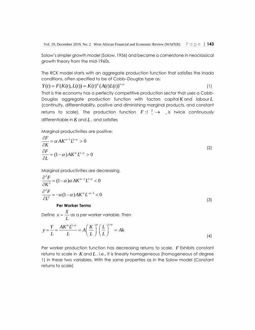
Vol. 19, December 2019, No. 2 West African Financial and Economic Review (WAFER) P a g e | 143
Solow’s simpler growth model (Solow, 1956) and became a cornerstone in neoclassical
growth theory from the mid-1960s.
The RCK model starts with an aggregate production function that satisfies the Inada
conditions, often specified to be of Cobb–Douglas type as: 1( ) ( ( ), ( )) ( ) ( ( ) ( ))Y t F K t L t K t A t L t (1)
That is the economy has a perfectly competitive production sector that uses a Cobb-
Douglas aggregate production function with factors capital K and labour L
(continuity, differentiability, positive and diminishing marginal products, and constant
returns to scale). The production function 2:F is twice continuously
differentiable in K and L , and satisfies
Marginal productivities are positive:
1 1
1
0
(1 ) 0
FAK L
K
FAK L
L
(2)
Marginal productivities are decreasing, 2
2 1
2
21
2
(1 ) 0
(1 ) 0
FAK L
K
FAK L
L
(3)
Per Worker Terms
Define X
xL
as a per worker variable. Then
11Y AK L K Ly A Ak
L L L L
(4)
Per worker production function has decreasing returns to scale. F Exhibits constant
returns to scale in K and L . i.e., it is linearly homogeneous (homogeneous of degree
1) in these two variables. With the same properties as in the Solow model (Constant
returns to scale)
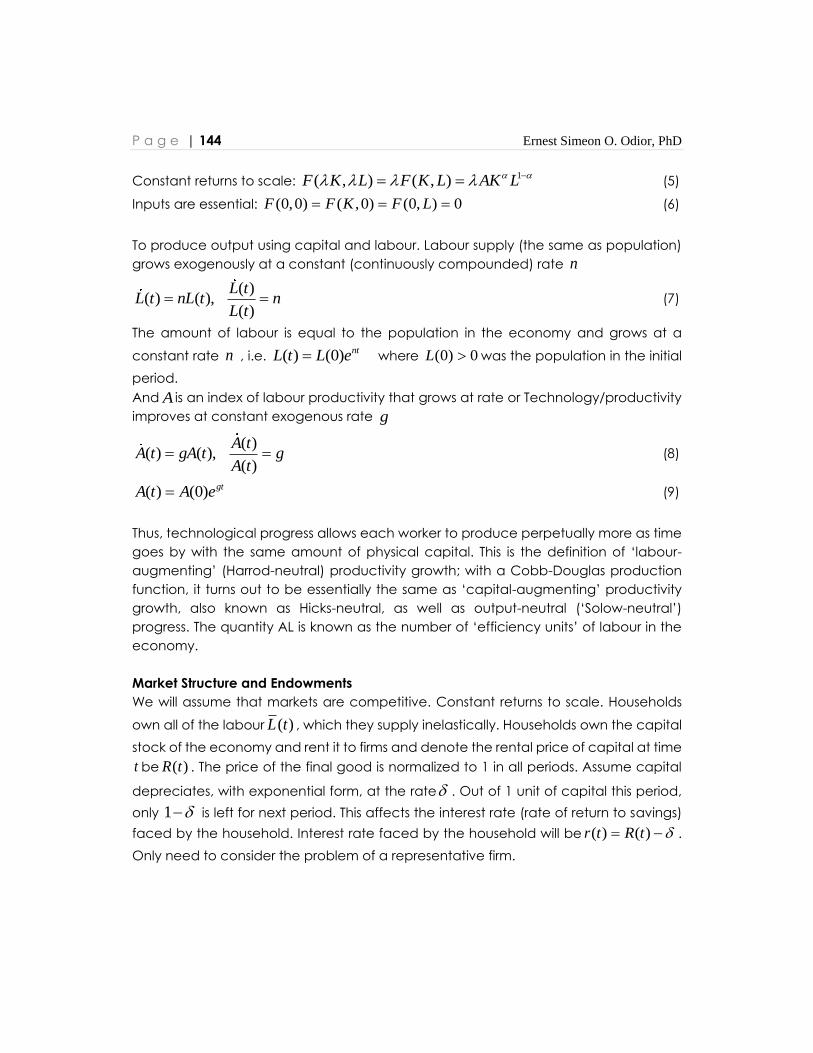
P a g e | 144 Ernest Simeon O. Odior, PhD
Constant returns to scale: 1( , ) ( , )F K L F K L AK L (5)
Inputs are essential: (0,0) ( ,0) (0, ) 0F F K F L (6)
To produce output using capital and labour. Labour supply (the same as population)
grows exogenously at a constant (continuously compounded) rate n
( )( ) ( ),
( )
L tL t nL t n
L t (7)
The amount of labour is equal to the population in the economy and grows at a
constant rate n , i.e. ( ) (0) ntL t L e where (0) 0L was the population in the initial
period.
And A is an index of labour productivity that grows at rate or Technology/productivity
improves at constant exogenous rate g
( )( ) ( ),
( )
A tA t gA t g
A t (8)
( ) (0) gtA t A e (9)
Thus, technological progress allows each worker to produce perpetually more as time
goes by with the same amount of physical capital. This is the definition of ‘labour-
augmenting’ (Harrod-neutral) productivity growth; with a Cobb-Douglas production
function, it turns out to be essentially the same as ‘capital-augmenting’ productivity
growth, also known as Hicks-neutral, as well as output-neutral (‘Solow-neutral’)
progress. The quantity AL is known as the number of ‘efficiency units’ of labour in the
economy.
Market Structure and Endowments
We will assume that markets are competitive. Constant returns to scale. Households
own all of the labour ( )L t , which they supply inelastically. Households own the capital
stock of the economy and rent it to firms and denote the rental price of capital at time
t be ( )R t . The price of the final good is normalized to 1 in all periods. Assume capital
depreciates, with exponential form, at the rate . Out of 1 unit of capital this period,
only 1 is left for next period. This affects the interest rate (rate of return to savings)
faced by the household. Interest rate faced by the household will be ( ) ( )r t R t .
Only need to consider the problem of a representative firm.
Vol. 19, December 2019, No. 2 West African Financial and Economic Review (WAFER) P a g e | 145
Firm Optimization
The stock market value of the firm is given by the discounted value of its cash flows:
( )
0(0) ( ( ), ( )) ( ) ( ) R tv F K t L t w t I t e dt
(10)
where ( )R t is the discounting factor given above and ( )I t is gross investment:
( ) ( ) ( )I t K t K t (11)
The firm maximizes (0)v subject to the capital accumulation constraint. Since there
are no adjustment costs on investment, the firm’s decision about factor inputs is
essentially a static one, i.e. the familiar marginal productivity conditions for labour and
capital hold:
( ( ), ( )) ( )LF K t L t w t (12)
( ( ), ( )) ( )KF K t L t r t (13)
By writing the production function in the intensive form, i.e.
( )( ( ) ,1
( )
K tf k t F
L t
, (14)
we can rewrite the marginal products of capital and labour as follows:
( ( ), ( )) ( ( ))KF K t L t f k t (15)
( ( ), ( )) ( ( )) ( ) ( ( ))LF K t L t f k t k t f k t (16)
Capital accumulation
The first key equation of the RCK model is the state equation for optimal capital
accumulation
( ) ( ( )) ( ) ( ) ( )k t f k t c t n k t (17)
( ) ( ( ))r t f k t (18)
Equation (17) is the Fundamental Differential Equation (FDE) for the capital stock.
Equation (18) shows that the real interest rate is the net marginal product of capital. A
non-linear differential equation akin to the Solow model, where. ( )c t is per capita
consumption, ( )k t is the capital-labour ratio, and ( )r t is the interest rate. k is capital
P a g e | 146 Ernest Simeon O. Odior, PhD
intensity (i.e., capital per worker), k is change in capital intensity over timedk
dt
, is c
consumption per worker, ( )f k is output per worker for a given, k and is the
depreciation rate of capital. Under the simplifying assumption that there is no
population growth, this equation states that investment, or increase in capital per
worker is that part of output which is not consumed, minus the rate of depreciation of
capital. Investment is, therefore, the same as savings. The main interest of the model is
the dynamics of capital intensity, the capital stock per unit of effective labour. Its
behaviour over time is given by the key equation of the Solow model:
The Solow Growth Model
The Solow model is a very important tool to understand the determinants of long term
growth. The main interest of the model is the dynamics of capital intensity, the capital
stock per unit of effective labour. Like the RCK model, the model starts with an
aggregate production function that satisfies the Inada conditions.
Dynamics of Capital
Assume constant and exogenous savings rates, (i.e. not a result of individual
optimization decision) and constant depreciation rate of capital ( ):
( ) ( ) ( )K t sY t K t (19)
Dynamics of capital per unit of effective labour, K
kAL
(20)
2
( ) ( )( ) ( ) ( ) ( ) ( )
( ) ( ) ( ) ( )
K t K tk t A t L t A t L t
A t L t A t L t (21)
( ) ( ) ( ) ( )
( ) ( ) ( ) ( ) ( ) ( )
K t K t L t A t
A t L t A t L t L t A t
(22)
( ) ( )( )( )
( ) ( )
sY t K tk t n g
A t L t
(23)
( ( )) ( ) ( )sf k t n g k t (24)
Equation (24) is the central equation of motion for the Solow model, the steady state.
This is a nonlinear first order differential equation in the variable ( )k t that describes the
Vol. 19, December 2019, No. 2 West African Financial and Economic Review (WAFER) P a g e | 147
process of capital accumulation in the economy: capital accumulation is the engine
of growth, since output per capita depends on the per-capita capital stock ( )k t .
According to Solow, to understand the growth process, we need to understand the
reasons for capital accumulation.
The first term, ( ( ))f k t is the actual investment in physical capital per unit of effective
labour. The second term, ( ) ( )n g k t is the effective depreciation of capital per
unit of effective labour. Steady-state (equilibrium) occurs at such value of capital per
effective labour, Steady state: a capital stock k
where, when reached, ( ) 0k t , that
is ( ) ( ) ) 0sf k n g k
4.0 Methodology
4.1 Analytical Technique
The analysis is based on a dynamic nonlinear optimal growth model. The primary
interest of this study is to use the first key equation of the RCK and Solow models to
find the growth path for capital accumulation and income over which the criterion
function is maximized among all feasible growth paths from 2017 to 2030. The systems
are based on aggregative behavioural equations. This study builds an internally
consistent, Dynamic General Equilibrium (DGE) framework, where forward-looking
agents make their optimal decisions, taking both current and future variables into
account. This entails dynamic equations involving today's and tomorrow's capital
stock etc. In other words this would bring us directly into the realm of income
dynamics over time, i.e., economic growth. In particular, we shall examine how the
period-by-period capital stock dynamics generate a growth path for the economy
and what happens to this growth trajectory in the long-run.
4.2 Specification Model
The analysis and specifications of the model are done with a standard
macroeconomic model structure derived from Kendrick & Taylor (1971). The model is
a non-linear programming (NLP) of seven (7) simultaneous complete equations. It is
model of optimum savings with a finite planning horizon. The empirical models
adopted in this study after a minor modification of (17), (18) and (24) are specified
as follows;
P a g e | 148 Ernest Simeon O. Odior, PhD
( )CAPB t : CapitalStock Balance Equation
( ) : ( 1) ( ) ( ) (1 ) ( )CAPB t CAP t INC t CON t CAP t (25)
(1/ )
( 1( )1( ) :
( )
INC tCAP t
t
(26)
( )INCD t : IncomeDefinition Equation
( )INCD t : ( ) ( ) ( )INC t t CAP t (27)
( ( ) 1)1( ) 0(1.06) tt tINC t INC (28)
( )PID t =Performance Index Definition Equation
( )PID t = (1 )( ) , ( 1) ( 1)PI t t r t CON t (29)
SAVR= Saving rate
1( ) 1( )
1( )
INC t CON tSAVR
INC t
(30)
( )CON t = Consumption Equation
1( ) 1( ) (1 ) 1( ) 1( 1)CON t INC t CAP t CAP t (31)
Definition of the Variables
( )CAP t = Capital stock in continuous time
( )INC t = Income in continuous time
( )PI t = Performance index in continuous time
( )CON t = Consumption in continuous time
Scalar
= rate of depreciation
= exponent on capital
n = labour force growth rate
= elasticity of substitution
z = technical progress
= welfare discount

Vol. 19, December 2019, No. 2 West African Financial and Economic Review (WAFER) P a g e | 149
0INC = initial per capita income
0CAP = initial capital
Parameter
= efficiency parameter in the production function
0 / 0INC CAP
( )r t = discount factor
(1 ( )) /(1 )( ) (1 ) tb tr t
( )t = production function parameter
( ( ) 1)( ) (1 )(1 ) ) tt tt n z
SAVR= Saving rate
4.3 Model Calibration
Thus, whether capital is at optimal to predict a higher growth rate of income, not
only temporarily, but also in the long run, depends on the flexibility of the values
of the scalar variables. In order to apply the RCK and Solow framework to the Nigerian
economy, the model is modified to fit the real data and to handle the policy issues.
The model is calibrated using the existing data for 2017 as a base year/period ( ( ))tb t ,
while the terminal period ( ( ))tt t is 2030. So the model is calibrated with respect to scalar
values (see Table 1)
Table 1: The Base Period (2017) Scalar Values
Rate of Depreciation 0.06
Exponent on Capital 0.25
n Labour Force Growth Rate 0.028
Capital Elasticity of Production 0.5
z Technical Progress 0.1
Welfare Discount 0.1
0INC Initial Income 3.454
0CAP Initial Capital 24.94431
Sources: NBS, WBI and Literature

P a g e | 150 Ernest Simeon O. Odior, PhD
4.4 Data Requirement and Sources
Data were obtained for rate of depreciation of the capital stock, exponential growth
of capital, labour force growth rate, elasticity of substitution between factors of
productions, technical progress, welfare discount, initial income and initial capital for
Nigeria. They are compiled from World Bank’s Development Indicator (WBI). Other
sources include data from the Nigerian National Bureau of Statistics (NBS) and from
literature.
Gross capital fixed formation is used as a proxy for capital stock with an initial value of
₦2494431 million. Nominal gross domestic product is used as a proxy for income at the
initial value of $345.4 billion (₦124,344 billion). Labour force growth rate is computed
from the Nigeria’s total labour force reported by the World Bank development
indicators of 2017, compiled from officially recognized sources with a value of
29,591,190 in 1990 to a value of 58,959,450 in 2017. Technical Progress is calculated as
the ratio of real GDP to working population or labour force, given as: Technical
Progress = In(Real GDP/Labour Force). Average rate of depreciation of the capital
stock of Nigeria increased from 0.03 rate in 1965 to 0.06 rate in 2017 growing at an
average annual rate of 1.83 %. (See the Database of Penn World Table 9.1).
Other scalars value were taken from literature as a result of many data scanty
problems in Nigeria, related to growth linkage. Welfare function of income or welfare
discount measured on a 0.1 scale is based on Hagenaars (1988). While, exponent on
capital is given as 0.25, which was subsequently confirmed by the National Bureau of
Economic Research to be 0.75 exponent of labour (Cobb & Douglas1928). Note, our
study assumes perfect competition and scale, that is α + β = 1, α and β can be shown
to be capital's and labour’s shares of output. Meaning that doubling the usage of
capital and labour will also double output.
4.5 Definition of Policy Simulation Experiments
The scenario involves using the sector properties that is the scalar values to run an
experiment to forecast an optimal and balanced growth path for capital and income
in order to ascertain the short, the medium and long-run optimal growth path for
capital and income. The "base year 2017" in the set serves as comparator.
The deviations are dynamic effects from 2017-2030. The normalized variables are
0 1( ) 1CAP t , 0 1( ) 1INC t , 0 1( ) 1CON t , since the model is homogeneous of
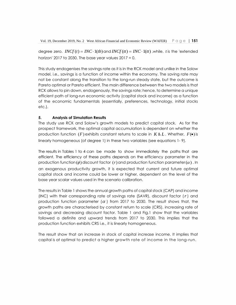
Vol. 19, December 2019, No. 2 West African Financial and Economic Review (WAFER) P a g e | 151
degree zero. ( ) 1( )INCf t INC tb and ( ) 1( )INCf tt INC tt ,while, t is the 'extended
horizon' 2017 to 2030. The base year values 2017 = 0.
This study endogenises the savings rate as it is in the RCK model and unlike in the Solow
model, i.e., savings is a function of income within the economy. The saving rate may
not be constant along the transition to the long-run steady state, but the outcome is
Pareto optimal or Pareto efficient. The main difference between the two models is that
RCK allows to pin down, endogenously, the savings rate; hence, to determine a unique
efficient path of long-run economic activity (capital stock and income) as a function
of the economic fundamentals (essentially, preferences, technology, initial stocks
etc.).
5. Analysis of Simulation Results
The study use RCK and Solow’s growth models to predict capital stock. As for the
prospect framework, the optimal capital accumulation is dependent on whether the
production function ( )F exhibits constant returns to scale in K & L . Whether, ( )F is
linearly homogeneous (of degree 1) in these two variables (see equations 1- 9).
The results in Tables 1 to 4 can be made to show immediately the paths that are
efficient. The efficiency of these paths depends on the efficiency parameter in the
production function ( ) discount factor ( )r and production function parameter ( ) . In
an exogenous productivity growth, it is expected that current and future optimal
capital stock and income could be lower or higher, dependent on the level of the
base year scalar values used in the scenario calibration.
The results in Table 1 shows the annual growth paths of capital stock (CAP) and income
(INC) with their corresponding rate of savings rate (SAVR), discount factor ( r ) and
production function parameter ( ) from 2017 to 2030. The result shows that, the
growth paths are characterised by constant return to scale (CRS), increasing rate of
savings and decreasing discount factor. Table 1 and Fig.1 show that the variables
followed a definite and upward trends from 2017 to 2030. This implies that the
production function exhibits CRS i.e., it is linearly homogeneous.
The result show that an increase in stock of capital increase income. It implies that
capital is at optimal to predict a higher growth rate of income in the long-run.
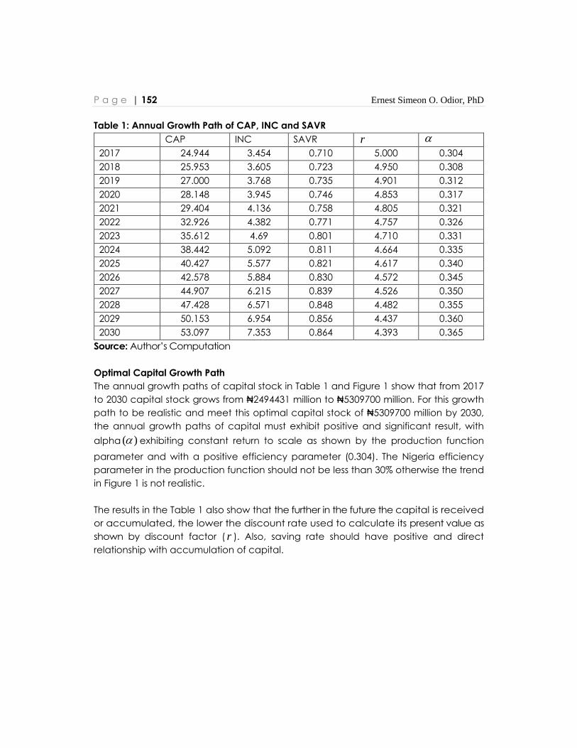
P a g e | 152 Ernest Simeon O. Odior, PhD
Table 1: Annual Growth Path of CAP, INC and SAVR
CAP INC SAVR r
2017 24.944 3.454 0.710 5.000 0.304
2018 25.953 3.605 0.723 4.950 0.308
2019 27.000 3.768 0.735 4.901 0.312
2020 28.148 3.945 0.746 4.853 0.317
2021 29.404 4.136 0.758 4.805 0.321
2022 32.926 4.382 0.771 4.757 0.326
2023 35.612 4.69 0.801 4.710 0.331
2024 38.442 5.092 0.811 4.664 0.335
2025 40.427 5.577 0.821 4.617 0.340
2026 42.578 5.884 0.830 4.572 0.345
2027 44.907 6.215 0.839 4.526 0.350
2028 47.428 6.571 0.848 4.482 0.355
2029 50.153 6.954 0.856 4.437 0.360
2030 53.097 7.353 0.864 4.393 0.365
Source: Author’s Computation
Optimal Capital Growth Path
The annual growth paths of capital stock in Table 1 and Figure 1 show that from 2017
to 2030 capital stock grows from ₦2494431 million to ₦5309700 million. For this growth
path to be realistic and meet this optimal capital stock of ₦5309700 million by 2030,
the annual growth paths of capital must exhibit positive and significant result, with
alpha ( ) exhibiting constant return to scale as shown by the production function
parameter and with a positive efficiency parameter (0.304). The Nigeria efficiency
parameter in the production function should not be less than 30% otherwise the trend
in Figure 1 is not realistic.
The results in the Table 1 also show that the further in the future the capital is received
or accumulated, the lower the discount rate used to calculate its present value as
shown by discount factor ( r ). Also, saving rate should have positive and direct
relationship with accumulation of capital.
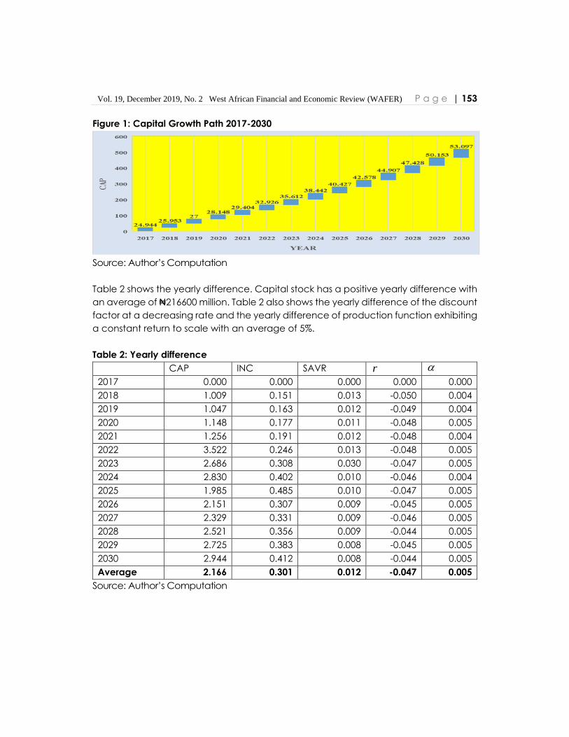
Vol. 19, December 2019, No. 2 West African Financial and Economic Review (WAFER) P a g e | 153
Figure 1: Capital Growth Path 2017-2030
Source: Author’s Computation
Table 2 shows the yearly difference. Capital stock has a positive yearly difference with
an average of ₦216600 million. Table 2 also shows the yearly difference of the discount
factor at a decreasing rate and the yearly difference of production function exhibiting
a constant return to scale with an average of 5%.
Table 2: Yearly difference
CAP INC SAVR r
2017 0.000 0.000 0.000 0.000 0.000
2018 1.009 0.151 0.013 -0.050 0.004
2019 1.047 0.163 0.012 -0.049 0.004
2020 1.148 0.177 0.011 -0.048 0.005
2021 1.256 0.191 0.012 -0.048 0.004
2022 3.522 0.246 0.013 -0.048 0.005
2023 2.686 0.308 0.030 -0.047 0.005
2024 2.830 0.402 0.010 -0.046 0.004
2025 1.985 0.485 0.010 -0.047 0.005
2026 2.151 0.307 0.009 -0.045 0.005
2027 2.329 0.331 0.009 -0.046 0.005
2028 2.521 0.356 0.009 -0.044 0.005
2029 2.725 0.383 0.008 -0.045 0.005
2030 2.944 0.412 0.008 -0.044 0.005
Average 2.166 0.301 0.012 -0.047 0.005
Source: Author’s Computation
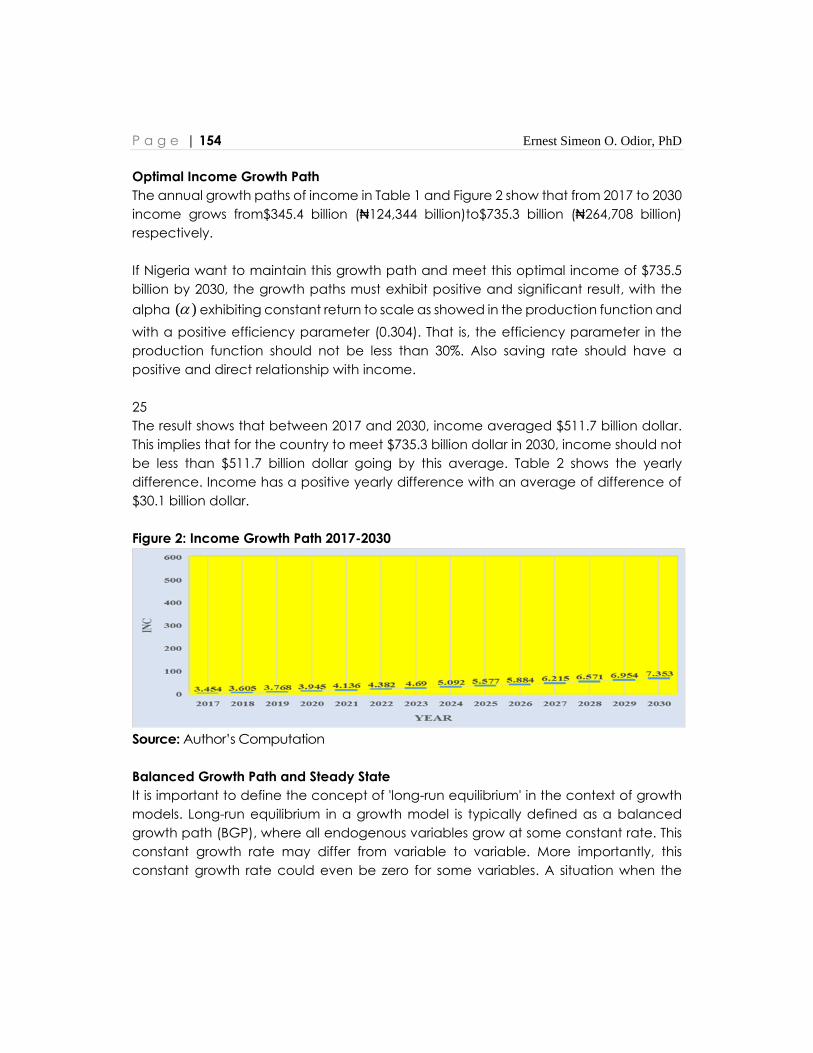
P a g e | 154 Ernest Simeon O. Odior, PhD
Optimal Income Growth Path
The annual growth paths of income in Table 1 and Figure 2 show that from 2017 to 2030
income grows from$345.4 billion (₦124,344 billion)to$735.3 billion (₦264,708 billion)
respectively.
If Nigeria want to maintain this growth path and meet this optimal income of $735.5
billion by 2030, the growth paths must exhibit positive and significant result, with the
alpha ( ) exhibiting constant return to scale as showed in the production function and
with a positive efficiency parameter (0.304). That is, the efficiency parameter in the
production function should not be less than 30%. Also saving rate should have a
positive and direct relationship with income.
25
The result shows that between 2017 and 2030, income averaged $511.7 billion dollar.
This implies that for the country to meet $735.3 billion dollar in 2030, income should not
be less than $511.7 billion dollar going by this average. Table 2 shows the yearly
difference. Income has a positive yearly difference with an average of difference of
$30.1 billion dollar.
Figure 2: Income Growth Path 2017-2030
Source: Author’s Computation
Balanced Growth Path and Steady State
It is important to define the concept of 'long-run equilibrium' in the context of growth
models. Long-run equilibrium in a growth model is typically defined as a balanced
growth path (BGP), where all endogenous variables grow at some constant rate. This
constant growth rate may differ from variable to variable. More importantly, this
constant growth rate could even be zero for some variables. A situation when the

Vol. 19, December 2019, No. 2 West African Financial and Economic Review (WAFER) P a g e | 155
constant growth rate is zero, it is called the steady state in the conventional dynamic
analysis (which is a special case of a BGP) (Mausumi, 2016). The standard RCK and
Solow model predicts that in the long run, economies converge to their steady state
equilibrium.
What determines the value of the BGP and steady state of *CAP and therefore
*INC
? The increase in rate of depreciation ( ) , the increase in labour force growth rate
( n ), and increase in technical progress ( z ). Intuitively, we think that more
depreciation should lead to less capital accumulation and lower steady-state *CAP
& *INC . Faster technological progress should allow economy to grow faster, both in
aggregate and in per capita terms. And more rapid population growth should allow
economy to grow faster because labour input is growing faster. That is, capital and
income grow at the rate of growth of technological progress and index of labour
productivity, z n , which is independent of SAVR. So each factor expands by z n
each year, with constant returns to scale. Growth in this model is “exogenous” capital
and income growth = z n are taken as given from outside the model.
Tables 3 and 4 shows the annual percentage growth rate and the deviation of each
year from the base year value (2017) and percentage deviation from base year values
(2017). Tables 3 and 4 show the balanced growth paths, steady state of capital stock,
income and saving rate values.
The annual percentage growth rate in Table 3 shows the annual percentage growth
rate of capital, income and the corresponding saving rate from 2017 to 2030. The result
shows that capital stock has a constant growth rate (on the BGP) from 2025 to 2030
and with an average annual growth rate of 5.53% from 2025 to 2030, while income has
a constant growth rate (on the BGP) from 2026 to 2030 and with an average annual
growth rate of 5.67% from 2026-2030 and with a corresponding rate of saving on the
BGP of 1.06% approximately.

P a g e | 156 Ernest Simeon O. Odior, PhD
Table 3: Annual Percentage Growth Rate
Year CAP INC SAVR
2017 0.00 0.00 0.00
2018 4.05 4.37 1.83
2019 4.03 4.52 1.66
2020 4.25 4.70 1.50
2021 4.46 4.84 1.61
2022 11.98 5.95 1.72
2023 8.16 7.03 3.89
2024 7.95 8.57 1.25
2025 5.16 9.52 1.23
2026 5.32 5.50 1.10
2027 5.47 5.63 1.08
2028 5.61 5.73 1.07
2029 5.75 5.83 0.94
2030 5.87 5.74 0.93
Average 2025-
2030 5.53 5.67 1.06
Source: Author’s Computation
Table 4 shows the deviation of each year from the base year value (2017) and their
corresponding percentage deviations. Table 4 shows capital stock deviation from the
base year value of ₦1548300 million in 2025, ₦1763400 million in 2026, ₦1996300 million
in 2027, ₦2248400 million in 2028, ₦2520900 million in 2029 and ₦2815300 million in 2030,
with their corresponding percentage deviation of 62%, 71%, 80%, 90%, 101% and 113%
respectively, while income has $212.3, $243.0, $276.1, $311.7, $350.0 and $389.9 billion
in 2025, 2026, 2027, 2028, 2029 and 2030, with their corresponding percentage
deviation of 61%, 70%, 80%, 90%, 101% and 113% respectively on the BGP with constant
saving rate along the transition to the long run steady state.

Vol. 19, December 2019, No. 2 West African Financial and Economic Review (WAFER) P a g e | 157
Table 4: Deviation and Percentage Deviation from Base Year Values (2017)
YEAR CAP INC SAVR
Deviation fr
om Base Ye
ar Value
% Deviati
on
Deviation fro
m Base Year
Value
% Devi
ation
Deviation fr
om Base Ye
ar Value
% Devi
ation
2017 0.000 0.000 0.000 0.000 0.000 0.000
2018 1.009 4.05 0.151 4.37 0.013 1.83
2019 2.056 8.24 0.314 9.09 0.025 3.52
2020 3.204 12.84 0.491 14.22 0.036 5.07
2021 4.460 17.88 0.682 19.75 0.048 6.76
2022 7.982 32.00 0.928 26.87 0.061 8.59
2023 10.668 42.77 1.236 35.78 0.091 12.82
2024 13.498 54.11 1.638 47.42 0.101 14.23
2025 15.483 62.07 2.123 61.46 0.111 15.63
2026 17.634 70.69 2.430 70.35 0.120 16.90
2027 19.963 80.03 2.761 79.94 0.129 18.17
2028 22.484 90.14 3.117 90.24 0.138 19.44
2029 25.209 101.06 3.500 101.33 0.146 20.56
2030 28.153 112.86 3.899 112.88 0.154 21.69
Source: Author’s Computation
6.0 Conclusion
The main objective of this research is to use the first key equations of the Ramsey-Cass-
Koopmans and Solow models to empirically project the likely optimal capital growth
path and the steady-state for Nigerian economy. Under the assumptions that the rate
of capital accumulation is independent of the saving rate, and they are positively
related. With a constant return to scale on the production function, that are
connected with the rate of exogenous technological progress. Also, the capital
growth path derived, offer the basis to analyse the long-run growth of income.
This study carried out a scenario and derived the balanced growth paths for capital
and income, in an exogenous growth setting for Nigeria, that are optimum with respect
to base period scalar values over a finite planning period 2017 to 2030, while 2017 in
the set, serves as comparator or base value.

P a g e | 158 Ernest Simeon O. Odior, PhD
The study reveals that the long-run capital accumulation considerably depends on the
values of the scalars. The result of the study shows that from 2025 to 2030, capital stock
and income grow at a constant rate. This show that the growth models predict a
unique steady-state capital and income level. In contrast to the suggestion that
capital accumulation plays a minor role in economic growth, the study find that
income has a large and statistically significant effect, but more importantly on its long-
run growth rate to the steady state be a function of the scalar values.
The forecasted growth paths show that capital and income followed some definite
and upward trends from 2017 to 2030 and that, an increase in capital accumulation,
also leads to an increase in incomes. This implies that optimal growth paths for capital
and income could only be sustain and achieve if and only if the aggregate production
function exhibit a constant or an increasing return to scales. Therefore, the
fundamental feature of these models is its competitive framework and its assumption
of constant returns to scale and diminishing returns.
Due to these assumptions, the two-capital neoclassical growth models predict that in
the absence of continuing improvements in technology, per capita growth must
eventually come to an end. But this prediction is not confirmed by facts.
Finally, this study provide overwhelming evidence that rapid and sustained capital and
income growth is critical to economic growth and the well-being of a nation.
Therefore, it is important to study and devise ways of promoting capitalist economic
development, because capital stock would be the engine of growth for developing
countries.
7.0 Policy Implication
The study shows the optimal traverse path for capital accumulation in Nigeria. It
presents evidence that an increase in capital stock predicts/leads to a higher income
growth, not only temporarily, but also in the long-run. The evidence that capital stock
has a long-run effect on growth rates is consistent with the main implication of some
exogenous growth models. This question is that can this upward trend be achievable
in any developing economy like Nigeria.
The fact that the derivatives are positive and consistent with one of the main
predictions of the neoclassical models, the study shows that the higher the
reinvestment rates, the higher the steady-state levels of capital. This have a vital policy
implication in the sense that the predictions of the neoclassical models depend on the
Vol. 19, December 2019, No. 2 West African Financial and Economic Review (WAFER) P a g e | 159
dynamics of technology and effective labour possessed by the economy. Therefore,
the optimal traverse path for capital stock growth in Nigeria is achievable only through
technological progress, the index of labour productivity and only if the aggregate
production function exhibits CRS. This implies that technological and labour
effectiveness should be the bases for capital accumulation and balanced growth
path for the Nigerian economy.
Government policymakers and planners around the world use capital accumulation
projections to gauge future demand for investment and to forecast future income that
would in turns affect economic growth. Capital accumulation projections help
policymakers craft policies that can be adapted for various projection scenarios,
because government need to look at the real factors that let countries create new
wealth. In most growth models, forecasting exercise was originally based on two major
components, capital and labour.
Capital accumulation is often suggested as a means for developing countries to
increase their long-term growth rates and the policy to be optimal capital must
be optimal at every stage. To increase capital accumulation it is necessary to:
increase savings ratios, maintain good banking system and system of loans,
avoid corruption, good infrastructure to make investment more worthwhile.
In general, contemporary growth theories and models have not been successfully
able to assess the determinants of growth, particularly in less developed counties.
Because, the definition and the measurement of theoretically predicted determinants
are much difficult and different in less developed countries from those in developed
countries. But the fact is that the primary origin of almost all growth theories and models
are the needs and the requirements of developed countries.
This gap can be bridged by paying attention to the dynamic effects of policies.
Considering that many less developed countries have had a growth experience that
was very far from the conditions of a steady-state, it is of great importance for policy
makers of less developed countries to find out the factors optimal capital. Equally
important, the derived capital growth equations are empirically testable provided that
data on capital stock of the economy are available. This means a potential for a new
method to test conditional convergence.
P a g e | 160 Ernest Simeon O. Odior, PhD
References
Cass, David (1965). Optimum Growth in an Aggregative Model of Capital
Accumulation. Review of Economic Studies. 32 (3): 233–240.
Central Bank of Nigeria (2017). Statistical Bulletin, Vol. 23, December, Abuja, Nigeria
Cobb, C. W.; Douglas, P. H. (1928). A Theory of Production , American Economic
Review. 18 (Supplement): 139–165.
Hagenaars A. J. M. (1988). The Perception of Poverty by Review by: Joop Hartog, The
Journal of Human Resources Vol. 23, No. 2, pp. 243-266, Published by: University
of Wisconsin Press
Hall R., C. I. Jones (1997). Why do Some Countries Produce So Much More per Worker
than Others? Quart J Econ 114: 83–116.
Hall, R. & C. Jones (1999). Why do some countries produce so much more output per
worker than others? Q. J. Econ., 114: 83-116.
Heston A, Summers R, & Aten B. (2002), Penn World Table Version 6.1. Philadelphia:
Centre for International Comparisons, the University of Pennsylvania.
Hoeffler, A. (2000). The augmented Solow model and the African growth debate.
Explaining Africa Economic Growth Performance Conference Series, CID
Working Paper No. 36.
Kendrick, D, & L. Taylor (1971). Numerical methods and Nonlinear Optimizing models
for Economic Planning. In Chenery, H B, Ed, Studies of Development Planning.
Harvard University Press.
Koopmans, T. C. (1965). On the Concept of Optimal Economic Growth". The Economic
Approach to Development Planning. Chicago: Rand McNally. pp. 225–287.
Mankiw NG, David R &Weil D. (1992). A contribution to the empirics of economic
growth. Quart J Econ 107: 407–437.
Mansour Zarra-N. & F. Hosainpour (2011). Review of Growth Models in Less Developed
Countries, the International Journal of Applied Economics and Finance Volume
5 (1): page 1-17
Mausumi Das (2016). Output Dynamics In the Long Run: Issues of Economic Growth,
lecture Notes, DSE
McQuinn K& Whelan K. (2007). Conditional convergence and the dynamics of the
capital-output ratio. J Econ Growth 12: 159–184.
National Bureau of Statistics (The Presidency) (2017). National Account Of Nigeria,
Federal Republic Of Nigeria, Plot 762, Independence Avenue, Central Business
District, Abuja.
Penn World Table 9.1 (2017). The Database
Vol. 19, December 2019, No. 2 West African Financial and Economic Review (WAFER) P a g e | 161
Pritchett, L. (2006). The quest continues. Fin. Develop., 43: 18-22.Ramsey, Frank P. (1928).
A Mathematical Theory of Saving. Economic Journal, 38 (152): 543–559
Rao, B. B. & A. Cooray (2009). How Useful Is Growth Literature for Policies in the
Developing Countries? MPRA Paper 14573. University Library of Munich,
Germany.
Rina Rosenblatt W. (2005), Optimal Capital Accumulation in a Stochastic Growth
Model under Loss Aversion, National Centre of Competence in Research
Financial Valuation and Risk Management, Working Paper No. 222
Solow, Robert M. (1956). A Contribution to the Theory of Economic Growth, Quarterly
Journal of Economics. Oxford Journals. 70 (1): 65–94
Takahashi T (2012) Capital Growth Paths of the Neoclassical Growth Model, PLos ONE
7(11)
World Bank Development Indicator (2017).
http://data.worldbank.org/indicator/Sp.Pop.Totl

P a g e | 162 Ernest Simeon O. Odior, PhD

P a g e | 163
POLICY BRIEF
ECONOMIC GROWTH AND EMISSIONS: TESTING THE ENVIRONMENTAL
KUZNETS CURVE HYPOTHESIS FOR ECOWAS COUNTRIES.
Prof. Douglason G. Omotor*1
Abstract
The relationship between economic growth and environmental sustainability is
premised on the environmental Kuznets curve (EKC) hypothesis. Two variants of
emissions related to contribute to environmental degradation in the extant literature
are sulfur dioxide (SO2) and carbon dioxide (CO2). Sulfur dioxide has the potential to
acidify rain, soil and lakes, and it can counteract some of the warming effects of
carbon dioxide. If unabated, the problem of environmental degradation could
aggravate and become unsustainable as income per capita increases. To stimulate
economic growth while minimizing environmental pollution, it is important policy
makers know much as to what drive these emissions in order to enact effective policy
and regulation that will support sustainable development.
For this much-needed information to be provided, this CEEPA study examines the
validity of the EKC hypothesis and the driving factors of SO2 and CO2 emissions in the
ECOWAS sub-region. Based on panel fixed and random effects estimation
techniques, the results show there is evidence of the validity for the two indicators of
environmental quality- SO2 and CO2 in the sub-region. These emissions in the ECOWAS
sub-region are induced by fuel processing and fuel combustion and rapid population
growth. In the light of this and the need to stimulate economic growth while
minimizing environmental pollution, there is need for strong institutions to enact
effective policy and rules and regulation that will support sustainable development.
*Corresponding author’s mail: [email protected] 1 West African Institute for Financial and Economic Management
2The research work was carried out with the aid of a grant from the Centre of Environmental
Economics and Policy in Africa (CEEPA – www.ceepa.co.za), financed by the Swedish
Development Cooperation Agency (SIDA) and the International Development Research
Center (IDRC). The work benefitted immensely from review comments of various resource
persons, among them, Wisdom Akpalu, David Starrett, Edwin Muchapondwa, Joe Cook, Marty
Lackat and other participants at the 25 – 29 August, 2014 CEEPA’s 15th Research and Training
Workshop, Pretoria, South Africa. I also wish to thank Sam Omoruyi for the editorial review.
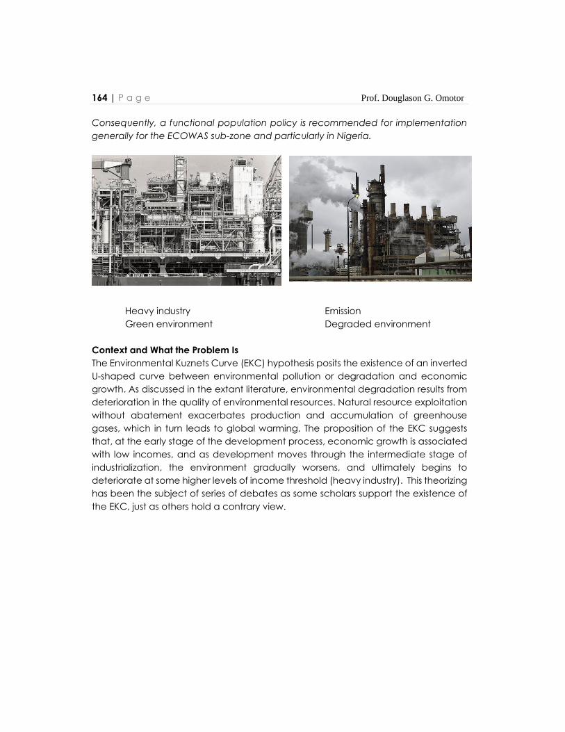
164 | P a g e Prof. Douglason G. Omotor
Consequently, a functional population policy is recommended for implementation
generally for the ECOWAS sub-zone and particularly in Nigeria.
Heavy industry Emission
Green environment Degraded environment
Context and What the Problem Is
The Environmental Kuznets Curve (EKC) hypothesis posits the existence of an inverted
U-shaped curve between environmental pollution or degradation and economic
growth. As discussed in the extant literature, environmental degradation results from
deterioration in the quality of environmental resources. Natural resource exploitation
without abatement exacerbates production and accumulation of greenhouse
gases, which in turn leads to global warming. The proposition of the EKC suggests
that, at the early stage of the development process, economic growth is associated
with low incomes, and as development moves through the intermediate stage of
industrialization, the environment gradually worsens, and ultimately begins to
deteriorate at some higher levels of income threshold (heavy industry). This theorizing
has been the subject of series of debates as some scholars support the existence of
the EKC, just as others hold a contrary view.
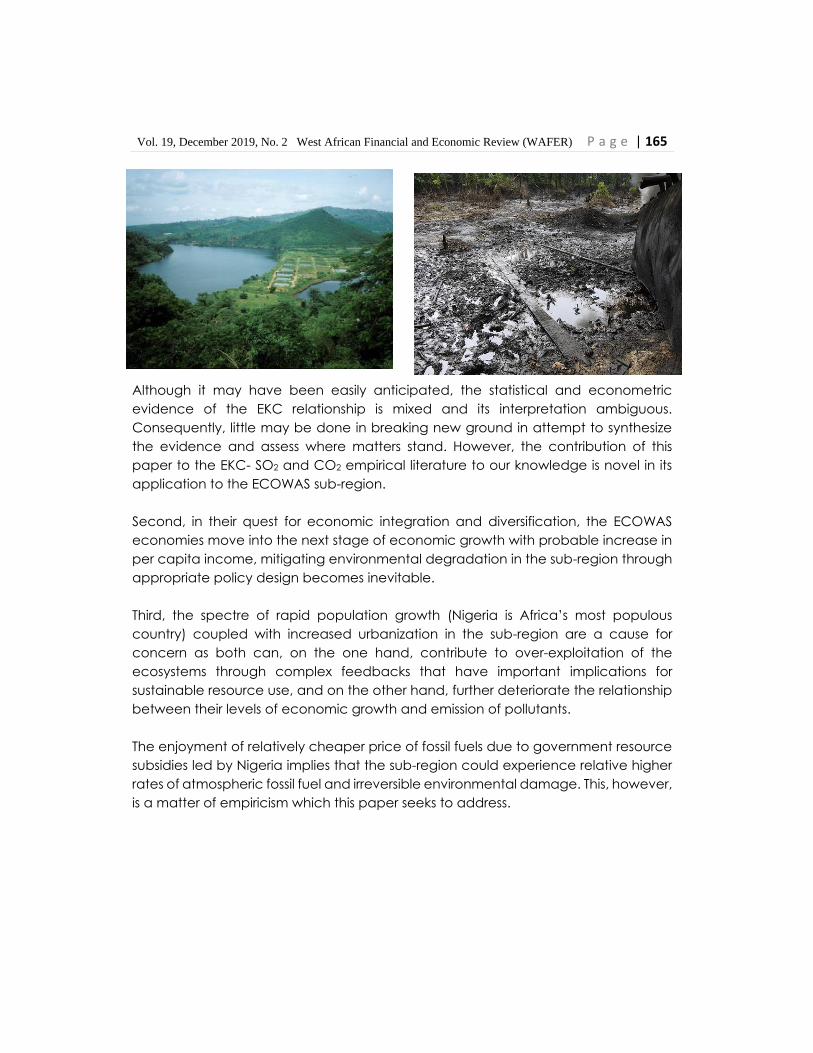
Vol. 19, December 2019, No. 2 West African Financial and Economic Review (WAFER) P a g e | 165
Although it may have been easily anticipated, the statistical and econometric
evidence of the EKC relationship is mixed and its interpretation ambiguous.
Consequently, little may be done in breaking new ground in attempt to synthesize
the evidence and assess where matters stand. However, the contribution of this
paper to the EKC- SO2 and CO2 empirical literature to our knowledge is novel in its
application to the ECOWAS sub-region.
Second, in their quest for economic integration and diversification, the ECOWAS
economies move into the next stage of economic growth with probable increase in
per capita income, mitigating environmental degradation in the sub-region through
appropriate policy design becomes inevitable.
Third, the spectre of rapid population growth (Nigeria is Africa’s most populous
country) coupled with increased urbanization in the sub-region are a cause for
concern as both can, on the one hand, contribute to over-exploitation of the
ecosystems through complex feedbacks that have important implications for
sustainable resource use, and on the other hand, further deteriorate the relationship
between their levels of economic growth and emission of pollutants.
The enjoyment of relatively cheaper price of fossil fuels due to government resource
subsidies led by Nigeria implies that the sub-region could experience relative higher
rates of atmospheric fossil fuel and irreversible environmental damage. This, however,
is a matter of empiricism which this paper seeks to address.
166 | P a g e Prof. Douglason G. Omotor
The State of the Environment in ECOWAS
The environment-development paradigm which shifted to sustainable development
began in the 1970s with the aim of formulating sustainable development policies that
will curtail emissions in the development process. The dialogues which followed the
discourse were to conserve the deteriorating environment and these resulted in a
series of government commitments covering at least nine treaties. This culminated in
a series of Treaties, Conventions, Multilateral Environmental Agreements and
Protocols. The ECOWAS sub-region and political leadership since the launch of the
ECOWAS Environmental Policy (2008) have displayed some signs of commitment and
appreciation of the consequences of environmental problems.
Profile of SO2 emissions in ECOWAS countries
A comparative examination of the evidence shows that SO2 emission in ECOWAS
countries ranked relatively lower than what obtained in some industrial countries. For
example, the mean or average SO2 concentration for the period, 1960-2005 for
Benin, Cote d’Ivoire, Ghana, Nigeria, Senegal and Togo stood at 2.5, 20.1, 18.8, 361.7,
20.5 and 202 Gg respectively; while those of China, Germany, Japan, UK and USA,
stood at 14224.6, 5597.1, 2057.6, 4070.7 and 22147.7, respectively.
A fundamental lesson deduced from the SO2 concentrations for the selected
ECOWAS countries when compared with the selected Industrial nations has been
that, ECOWAS countries may have the benefit of learning early and by involving in
environmental activism and awareness may not need to wait for too long for per
capita income to improve to the levels recorded in industrial nations before they
begin to appreciate cleaner environment.
Profile of CO2 emissions in ECOWAS countries
It has been argued that, given the current level of economic development in the
ECOWAS sub-region, recorded carbon per capita may be rising in recent years. This
fear reflects the fact that as the region’s economy grows, carbon dioxide per capita
may escalate as a result of industrialization. In 1960 for instance, carbon dioxide per
capita rate of increase per year in the sub-region was 0.71 PPM (parts per million)
and by 2005, the rate of increase stood at 2.14 PPM per year. As the sub-region’s
quest for rapid industrialization increases, the ECOWAS may do better by deliberately
stepping up measures to curb the trend towards increased carbon intensity.

Vol. 19, December 2019, No. 2 West African Financial and Economic Review (WAFER) P a g e | 167
Study Framework and Methodology
The general objective has been to relate environmental degradation to economic
growth measured by increases in per capita income and to establish the validity of
the EKC hypothesis of an inverted U-shape for the two indicators of environmental
quality- SO2 and CO2. The study uses annual panel data for selected ECOWAS
countries to estimate the environmental Kuznets curves. The data are obtained from
publications of the World Bank and the African Development Bank, among others.
Study Findings
The results are in tandem with the EKC Hypothesis for the two environmental
indicators- SO2 and CO2 using ECOWAS sample data. The computed income per
capita turning point of the SO2 Fixed Effects model average $5,650 dollars over the
period. The turning point value on average is higher than the region’s average gross
domestic product (GDP) per capita which ranges from USD 800 in Niger to USD 4,400
in Cape Verde. For carbon dioxide, perverse turning point was established.
The major drivers of SO2 in the sub-region are fuel processing and fuel combustion led
by Nigeria. For CO2 emissions, it is driven by rapid population growth which is equally
induced by Nigeria. The polity variable which interacted significantly with the income
variable to create the inverted-U shape EKC signals the importance of public
institutions on environmental quality.
Policy Recommendation
From the foregoing brief discussions, some policy implications arise from the findings
of this study. First, the existence of an EKC for the two indicators of environmental
quality implies that policy prescription needed to abate these form of environmental
emissions, should be such which enhances growth and incomes. Second, and arising
from the first, the need to stimulate economic growth while minimizing environmental
pollution requires strong institutions to enact and implement effective policy, rules
and regulation that will support sustainable development. Third, the concern for
policy making should be how the productive process of pollution emitting firms and
those of other economic agents whose actions relate to the environment for
instance, can be managed in the interest of the environment. The study further
recommends implementation of a functional population policy generally for the
ECOWAS sub-zone and particularly for Nigeria.

168 | P a g e Prof. Douglason G. Omotor
Lagos Makoko Water Village with over 85,000 inhabitants Lagos Eko, Nigeria
CORRESPONDENCE Enquires and/or comments on the WAFER and published articles should be addressed to: The Editor in-chief, West African Financial and Economic Review West African Institute for Financial and Economic Management, CBN Leaning Centre P.M.B 2001, Satellite Town, Lagos, Nigeria. Tel: +234 8054407387, +234 8080456007, +234 8146964647 E-mail: [email protected] www.waifem-cbp.org

KAS: 08056124959