wage dynamics working paper series network … · working paper series no 1184 / april 2010 ... as...

Work ing PaPer Ser i e Sno 1184 / aPr i L 2010

CoStS, demand,

and ProduCer

PriCe ChangeS

by Claire Loupias and Patrick Sevestre

WAGE DYNAMICSNETWORK

WORKING PAPER SER IESNO 1184 / APR I L 2010

In 2010 all ECB publications

feature a motif taken from the

€500 banknote.

COSTS, DEMAND,

AND PRODUCER PRICE CHANGES1

by Claire Loupias 2 and Patrick Sevestre 3

1 This study was initiated in the context of the Eurosystem Inflation Persistence Network. We are grateful to R. Ricart and B. Fougier for having provided

us with the series of the monthly manufacturing business surveys of the Banque de France, as well as to the DARES (Direction de l. Animation de la

Recherche, des Études et des Statistiques, French Ministry of Labor), for having provided the data about wages. Thanks also to P. Franceschi and

A. Gubian, from the ACOSS (Agence Centrale des Organismes de Sécurité Sociale) who gave us access to the monthly industry level wage bill

series used in previous versions of this paper. We are also strongly indebted to T. Heckel, H. Le Bihan, E. Gautier and to colleagues from the

Wage Dynamics Network of the Eurosystem for helpful discussions. We would like to thank also the participants to seminars at INRA

(Rennes), at the Université Paris 1 – Panthéon Sorbonne, at Monash University, to the AFSE annual conference (Paris), the JMA conference

(Fribourg) and the WDN conference (Frankfurt) for their comments and suggestions, with a special mention to E. Wasmer and T. Bewley.

Last but not least, we are much grateful to L. Baudry and S. Tarrieu for their wonderful research assistance. The usual disclaimer applies.

In particular, the views expressed herein are those of the authorsand do not necessarily reflect those of the Banque de France.

2 Claire Loupias was belonging to the Research Department of the Banque de France when the first draft

of this paper was written. EPEE, TEPP (FR-CNRS 3126) Université d.Evry Val d.Essonney.

3 Corresponding author : Banque de France, SAMIC-DEMS-DGEI and Paris School of Economics,

Université de Paris I – Panthéon Sorbonne, e-mail : [email protected]

This paper can be downloaded without charge from http://www.ecb.europa.eu or from the Social Science Research Network electronic library

at http://ssrn.com/abstract_id=1588767.

NOTE: This Working Paper should not be reported as representing the views of the European Central Bank (ECB). The views expressed are those of the authors

and do not necessarily reflect those of the ECB.

WAGE DYNAMICS

NETWORK

© European Central Bank, 2010

AddressKaiserstrasse 2960311 Frankfurt am Main, Germany

Postal addressPostfach 16 03 1960066 Frankfurt am Main, Germany

Telephone+49 69 1344 0

Internethttp://www.ecb.europa.eu

Fax+49 69 1344 6000

All rights reserved.

Any reproduction, publication and reprint in the form of a different publication, whether printed or produced electronically, in whole or in part, is permitted only with the explicit written authorisation of the ECB or the authors.

Information on all of the papers published in the ECB Working Paper Series can be found on the ECB’s website, http://www.ecb.europa.eu/pub/scientific/wps/date/html/index.en.html

ISSN 1725-2806 (online)

Wage Dynamics Network

This paper contains research conducted within the Wage Dynamics Network (WDN). The WDN is a research network consisting of economists from the European Central Bank (ECB) and the national central banks (NCBs) of the EU countries. The WDN aims at studying in depth the features and sources of wage and labour cost dynamics and their implications for monetary policy. The specific objectives of the network are: i) identifying the sources and features of wage and labour cost dynamics that are most relevant for monetary policy and ii) clarifying the relationship between wages, labour costs and prices both at the firm and macro-economic level.

The refereeing process of this paper has been co-ordinated by a team composed of Gabriel Fagan (ECB,

Bihan (Banque de France) and Thomas Mathä (Banque centrale du Luxembourg).

form, to encourage comments and suggestions prior to final publication. The views expressed in the paper are the author’s own and do not necessarily reflect those of the ESCB.

The paper is released in order to make the results of WDN research generally available, in preliminary

The WDN is chaired by Frank Smets (ECB). Giuseppe Bertola (Università di Torino) and Julián Messina

chairperson), Philip Vermeulen (ECB), Giuseppe Bertola, Julián Messina, Jan Babecký (CNB), Hervé Le

(World Bank and University of Girona) act as external consultants and Ana Lamo (ECB) as Secretary.

3ECB

Working Paper Series No 1184April 2010

Abstract 4

Non-technical summary 5

1 Introduction 7

2 Changes in prices versus changes in the fi rms environment: some basic facts 9

3 The model: a simple state-dependent pricing model 13

3.1 The optimal (frictionless) price 13

3.2 The desired price change 14

3.3 The price change rule 4 The dataset 17

4.1 Data sources 18

4.2 The econometric database 21

5 Estimation results 23

5.1 The econometric model 23

5.2 The baseline model estimates 26

5.3 Are current and recent variations in the environment more likely to induce price changes? 30

5.4 What about asymmetries? 34

6 Conclusion 36

7 References 36

Appendix 41

Tables 47

CONTENTS

16

4ECBWorking Paper Series No 1184April 2010

5ECB


7ECB


9ECB


11ECB


13ECB


15ECB


17ECB


19ECB


21ECB


23ECB


25ECB


27ECB


29ECB


31ECB


33ECB


35ECB


37ECB


39ECB


41ECB


Table A1: State-dependent model estimates

Coeff Z-stat Coeff Z-stat Coeff Z-stat Coeff Z-stat Coeff Z-statcum_ii_price 0.041 17.82 0.127 29.36 0.144 28.48 0.181 29.06 0.195 27.06cum_wage -0.003 -1.10 0.001 0.07 -0.001 -0.07 -0.015 -1.45 -0.010 -0.83cum_prod 0.008 4.90 0.032 9.63 0.025 6.62 0.046 9.12 0.038 6.69cum_sect_price 0.013 4.59 0.105 18.99 0.110 17.36 0.109 19.18 0.117 17.95vat_2000 0.122 1.79 0.080 1.17 0.095 1.36 0.084 1.19 0.098 1.35vat_2000_2 -0.051 -1.27 0.009 0.22 -0.001 -0.03 0.008 0.20 0.000 0.00Euro_2002 0.042 0.85 0.043 0.85 0.047 0.91 0.037 0.71 0.038 0.71Euro_2002_2 -0.101 -4.73 -0.018 -0.81 -0.020 -0.88 -0.005 -0.21 -0.009 -0.39q1 -2.274 -95.92 -2.188 -83.52 -2.368 -65.48 -1.380 -57.72 -1.481 -42.48q2 -1.451 -71.03 -1.362 -58.64 -1.467 -43.77q3 1.232 61.35 1.356 58.53 1.429 42.79 1.341 56.30 1.425 41.09q4 2.031 90.29 2.174 85.22 2.291 64.90sect_c1 -0.032 -0.85 -0.086 -2.24 -0.103 -1.52 -0.086 -2.23 -0.110 -1.60sect_c2 -0.243 -6.49 -0.199 -5.27 -0.213 -3.08 -0.227 -5.90 -0.246 -3.52sect_c3 -0.057 -1.50 -0.279 -7.03 -0.271 -3.87 -0.279 -6.94 -0.291 -3.98sect_c4 0.011 0.40 -0.078 -2.79 -0.078 -1.56 -0.107 -3.73 -0.105 -2.01sect_d0 -0.148 -5.00 -0.243 -7.87 -0.294 -5.27 -0.250 -7.81 -0.318 -5.39sect_e1 -0.189 -5.11 -0.262 -6.79 -0.335 -4.71 -0.272 -6.95 -0.360 -4.91sect_e2 -0.019 -0.84 -0.125 -5.38 -0.132 -3.17 -0.141 -5.93 -0.148 -3.39sect_e3 -0.135 -3.10 0.036 0.80 0.023 0.30 0.038 0.83 0.032 0.41sect_f1 0.012 0.44 -0.101 -3.75 -0.082 -1.63 -0.154 -5.60 -0.148 -2.86sect_f2 -0.171 -5.50 -0.206 -6.57 -0.209 -3.49 -0.254 -7.95 -0.244 -3.98sect_f3 -0.123 -5.43 -0.104 -4.54 -0.084 -1.96 -0.122 -5.23 -0.095 -2.10sect_f4 0.033 1.51 -0.056 -2.49 -0.066 -1.63 -0.073 -3.18 -0.074 -1.75sect_f5 0.078 3.61 -0.047 -2.14 -0.056 -1.37 -0.061 -2.67 -0.066 -1.58sect_f6 -0.292 -6.09 -0.344 -7.10 -0.357 -4.68 -0.378 -7.66 -0.381 -4.86year_1999 0.027 0.74 0.078 2.06 0.075 1.81 0.093 2.40 0.098 2.30year_2000 0.221 8.14 0.143 5.08 0.156 4.96 0.131 4.59 0.150 4.65year_2001 -0.008 -0.34 0.011 0.45 0.018 0.67 -0.002 -0.08 0.003 0.11year_2002 -0.105 -4.66 -0.027 -1.18 -0.013 -0.52 -0.022 -0.93 -0.011 -0.43year_2003 -0.203 -10.67 -0.106 -5.43 -0.095 -4.45 -0.097 -4.89 -0.090 -4.11year_2004 0.042 2.29 0.037 1.97 0.043 2.19 0.043 2.26 0.052 2.58y_0 0.032 1.95 0.048 2.161st stage residualscum_ii_price -0.114 -22.60 -0.106 -18.87 -0.161 -22.20 -0.142 -17.50cum_wage 0.012 1.51 0.009 1.07 0.028 2.55 0.011 0.92cum_prod -0.028 -7.38 -0.018 -4.37 -0.042 -7.13 -0.029 -4.49cum_sect_price -0.119 -18.44 -0.117 -16.40 -0.126 -18.85 -0.126 -16.99rho=su/(su+sw) 0.128 22.56 0.135 22.17LogLNumber of obs.

Ordered probit with 5 outcomes

51,067


51,06735,482

Simple Probitmethod for

51,067

Rivers-Vuong

51,067

endogenous var. unobs. Heterog. endogenous var. unobs. Heterog.

-35,013 -34,074 -30,351 -29,41251,067

Rivers-Vuong andWooldridge for method for Wooldridge for

Rivers-VuongRivers-Vuong and


with

sect_b0 Agri-food industriessect_c1 Clothing and leather goodssect_c2 Publishing and printingsect_c3 Pharmaceuticals, perfumes and cleaning productssect_c4 Household equipmentsect_d0 Automotive industrysect_e1 Shipbuilding, aircraft and rail constructionsect_e2 Mechanical equipmentsect_e3 Electrical and electronic equipmentsect_f1 Mineral productssect_f2 Textilessect_f3 Wood and papersect_f4 Chemicals, rubber and plasticssect_f5 Metalwork and fabricated metal productssect_f6 Electrical and electronic components

and with rho=su/(su+sw) the share of the firm specific effect variance in the total variance.

sect_b0 is the reference sector in all regressions below.

43ECB


Table A2: Estimates of a flexible dynamic model

Coeff Z-stat Coeff Z-stat Coeff Z-stat Coeff Z-stat Coeff Z-statii_price 0.434 49.52 1.100 5.07 1.188 5.32 1.623 5.72 1.737 5.92ii_price(-1) -0.069 -5.75 -0.266 -2.51 -0.265 -2.43 -0.361 -2.86 -0.361 -2.77ii_price(-2) -0.011 -0.80 -0.056 -1.51 -0.042 -1.10 -0.105 -2.07 -0.092 -1.77ii_price(-3) 0.020 1.34 0.051 1.80 0.071 2.44 0.060 1.64 0.078 2.06remain_cum_iip -0.010 -2.79 0.022 1.15 0.043 2.18 0.049 2.05 0.067 2.65wage 0.024 3.28 0.170 7.05 0.181 7.31 0.213 5.38 0.231 5.63wage(-1) 0.000 -0.04 0.012 1.08 0.011 1.00 0.001 0.05 0.005 0.25wage(-2) 0.009 1.01 0.018 1.47 0.018 1.41 -0.007 -0.34 -0.002 -0.10wage(-3) -0.004 -0.41 0.005 0.36 0.004 0.33 -0.054 -2.24 -0.051 -2.01remain_cum_wage 0.009 2.71 0.046 3.59 0.048 3.53 0.004 0.22 0.015 0.79prod 0.043 9.32 0.039 0.91 0.035 0.80 0.037 0.55 0.039 0.57prod(-1) 0.006 1.05 0.019 2.41 0.014 1.78 0.025 2.31 0.021 1.83prod(-2) 0.002 0.30 0.021 2.88 0.016 2.11 0.042 3.60 0.037 3.06prod(-3) -0.009 -1.51 -0.002 -0.26 -0.009 -1.06 -0.010 -0.73 -0.019 -1.32remain_cum_prod 0.007 3.06 0.039 6.46 0.033 5.00 0.058 6.14 0.052 5.02sect_price 0.238 18.11 0.148 10.58 0.163 11.20 0.160 11.18 0.179 11.92sect_price(-1) 0.022 1.36 0.107 4.66 0.118 4.98 0.103 4.39 0.115 4.76sect_price(-2) 0.003 0.14 0.102 4.29 0.110 4.46 0.112 4.59 0.124 4.88sect_price(-3) -0.011 -0.55 0.103 3.73 0.114 3.98 0.112 3.96 0.126 4.29remain_cum_price -0.006 -1.52 0.055 4.46 0.055 4.17 0.059 4.63 0.063 4.59vat_2000 0.087 1.26 0.069 0.96 0.078 1.07 0.082 1.11 0.092 1.21vat_2000_2 -0.141 -3.45 -0.134 -3.01 -0.152 -3.30 -0.131 -2.91 -0.145 -3.09Euro_2002 0.064 1.24 0.041 0.64 0.047 0.71 0.062 0.97 0.066 1.01Euro_2002_2 -0.073 -3.35 -0.020 -0.89 -0.017 -0.72 -0.008 -0.33 -0.005 -0.22q1 -2.315 -95.64 -2.194 -76.48 -2.373 -62.19 -1.389 -53.03 -1.480 -40.47q2 -1.473 -70.60 -1.348 -52.22 -1.447 -40.79 1.427 54.49 1.535 41.99q3 1.308 63.61 1.460 56.40 1.551 43.70q4 2.174 92.91 2.349 82.35 2.487 65.87sect_c1 -0.031 -0.81 -0.103 -2.52 -0.125 -1.80 -0.072 -1.76 -0.097 -1.37sect_c2 -0.264 -6.94 -0.239 -6.19 -0.253 -3.53 -0.249 -6.31 -0.267 -3.64sect_c3 -0.054 -1.40 -0.233 -5.34 -0.230 -3.18 -0.216 -4.80 -0.232 -3.10sect_c4 0.010 0.34 -0.080 -2.71 -0.087 -1.68 -0.111 -3.63 -0.107 -1.94sect_d0 -0.169 -5.60 -0.303 -9.16 -0.370 -6.49 -0.293 -8.45 -0.367 -6.02sect_e1 -0.184 -4.88 -0.289 -7.02 -0.364 -5.03 -0.248 -5.82 -0.337 -4.46sect_e2 -0.058 -2.54 -0.201 -7.24 -0.214 -4.76 -0.202 -7.34 -0.220 -4.79sect_e3 -0.073 -1.66 0.012 0.24 -0.002 -0.03 0.056 1.15 0.057 0.72sect_f1 -0.015 -0.56 -0.102 -3.57 -0.096 -1.83 -0.157 -5.32 -0.161 -2.99sect_f2 -0.156 -4.95 -0.186 -5.73 -0.183 -2.93 -0.215 -6.46 -0.200 -3.17sect_f3 -0.137 -6.01 -0.141 -5.80 -0.131 -2.90 -0.149 -6.16 -0.122 -2.66sect_f4 -0.006 -0.25 -0.124 -4.49 -0.149 -3.33 -0.133 -4.90 -0.148 -3.29sect_f5 -0.008 -0.37 -0.143 -4.69 -0.165 -3.63 -0.156 -5.30 -0.173 -3.81sect_f6 -0.298 -6.11 -0.346 -7.03 -0.367 -4.78 -0.388 -7.71 -0.397 -5.02year_1999 -0.057 -1.52 -0.045 -0.86 -0.049 -0.88 -0.086 -1.53 -0.082 -1.38year_2000 0.134 4.80 0.046 1.16 0.057 1.33 -0.012 -0.27 0.000 0.01year_2001 0.061 2.52 0.134 4.48 0.159 4.87 0.126 4.10 0.150 4.47year_2002 -0.108 -4.70 -0.033 -1.35 -0.008 -0.31 -0.026 -1.05 -0.005 -0.17year_2003 -0.184 -9.47 -0.112 -5.50 -0.090 -4.04 -0.096 -4.61 -0.077 -3.36year_2004 -0.051 -2.67 -0.141 -3.51 -0.146 -3.50 -0.137 -3.58 -0.140 -3.52

method for Wooldridge for method for Wooldridge forendog. var. unobs. heterog. endog. var. unobs. heterog.

Ordered probit with 5 outcomes Ordered probit with 3 outcomesSimple Probit Rivers-Vuong Rivers-Vuong and Rivers-Vuong Rivers-Vuong and


Table A2 (cont.): Estimates of a flexible dynamic model

Coeff Z-stat Coeff Z-stat Coeff Z-stat Coeff Z-stat Coeff Z-staty_0 0.043 2.64 0.060 2.721st stage residualsii_price -0.708 -3.26 -0.753 -3.37 -1.101 -3.88 -1.162 -3.96ii_price(-1) 0.061 0.57 0.071 0.65 0.066 0.51 0.083 0.62ii_price(-2) 0.019 0.47 0.019 0.45 0.014 0.24 0.019 0.33ii_price(-3) -0.063 -1.94 -0.068 -2.03 -0.099 -2.28 -0.099 -2.20remain_cum_iip -0.037 -1.92 -0.045 -2.27 -0.061 -2.48 -0.063 -2.45wage -0.157 -6.21 -0.170 -6.52 -0.227 -5.37 -0.244 -5.57wage(-1) 0.008 0.44 0.006 0.32 0.044 1.26 0.016 0.45wage(-2) 0.032 1.70 0.024 1.22 0.150 4.45 0.112 3.19wage(-3) 0.027 1.43 0.017 0.84 0.149 4.32 0.117 3.25remain_cum_wage -0.029 -2.21 -0.034 -2.45 0.015 0.84 -0.003 -0.15prod 0.003 0.07 0.005 0.11 0.022 0.32 0.018 0.25prod(-1) -0.068 -5.33 -0.052 -3.93 -0.094 -4.67 -0.076 -3.60prod(-2) -0.065 -5.55 -0.050 -4.10 -0.113 -5.98 -0.096 -4.88prod(-3) -0.021 -1.77 -0.006 -0.52 -0.030 -1.53 -0.011 -0.54remain_cum_prod -0.036 -5.58 -0.028 -4.00 -0.054 -5.29 -0.042 -3.85sect_price(-1) -0.240 -6.90 -0.240 -6.71 -0.257 -7.05 -0.258 -6.84sect_price(-2) -0.175 -4.99 -0.173 -4.81 -0.198 -5.40 -0.198 -5.24sect_price(-3) -0.185 -4.97 -0.203 -5.27 -0.218 -5.66 -0.239 -5.96remain_cum_price -0.061 -4.70 -0.055 -3.98 -0.067 -5.00 -0.063 -4.42rho=su/(su+sw) 0.128 22.76 0.134 22.29LogL

Rivers-Vuong Rivers-Vuong and

endog. var. unobs. heterog. endog. var. unobs. heterog.method for Wooldridge for method for Wooldridge for

-29,022

Ordered probit with 3 outcomesSimple Probit


-34,068 -33,632 -32,676

Rivers-Vuong Rivers-Vuong and

-28,086

45ECB


Table A3: Estimates of a model with asymmetries

Coeff Z-stat Coeff Z-stat Coeff Z-stat Coeff Z-statii_price -0.355 -0.74 1.370 5.87 0.282 0.38 1.530 4.33ii_price(-1) 0.232 1.17 -0.271 -2.29 0.091 0.34 -0.225 -1.46ii_price(-2) 0.041 0.55 -0.046 -0.66 -0.001 -0.01 -0.025 -0.26ii_price(-3) 0.068 0.85 0.085 1.19 0.014 0.12 0.135 1.45remain_cum_iip 0.132 1.95 0.022 0.35 0.182 1.39 0.030 0.33wage 0.988 1.54 0.210 6.21 2.432 2.66 0.400 4.30wage(-1) -0.067 -2.30 0.034 2.90 -0.054 -1.07 0.006 0.23wage(-2) -0.027 -0.83 0.040 2.46 -0.071 -1.20 0.052 1.46wage(-3) -0.027 -0.62 0.035 1.17 -0.066 -1.00 0.039 0.76remain_cum_wage -0.016 -0.39 0.054 2.75 -0.240 -1.87 0.017 0.71prod 0.298 2.42 -0.223 -2.00 0.193 1.02 -0.116 -0.49prod(-1) -0.050 -1.50 0.065 3.24 -0.015 -0.28 0.070 2.00prod(-2) -0.005 -0.25 0.047 2.91 0.018 0.54 0.071 2.56prod(-3) -0.031 -1.25 0.027 1.33 -0.009 -0.27 0.022 0.66remain_cum_prod -0.100 -1.40 0.119 3.14 -0.061 -0.58 0.119 2.12sect_price 0.039 1.37 0.204 10.08 0.047 1.61 0.223 10.54sect_price(-1) 0.100 2.42 0.077 1.66 0.070 1.63 0.161 3.20sect_price(-2) -0.037 -0.77 0.221 5.15 -0.003 -0.07 0.226 5.07sect_price(-3) 0.025 0.35 0.167 2.59 0.058 0.90 0.158 2.47remain_cum_price 0.019 1.01 0.058 1.88 0.004 0.21 0.096 2.85vat_2000 0.028 0.36 0.196 1.94vat_2000_2 -0.122 -2.43 -0.090 -1.81Euro_2002 0.081 1.16 0.068 1.05Euro_2002_2 -0.058 -2.09 -0.007 -0.23q1 -1.971 -21.72 -1.142 -11.89q2 -1.117 -12.46q3 1.697 18.89 1.679 17.45q4 2.585 28.46sect_c1 -0.140 -1.43 -0.132 -1.55sect_c2 -0.077 -1.23 -0.151 -2.19sect_c3 -0.226 -2.13 -0.250 -2.53sect_c4 0.015 0.26 -0.041 -0.75sect_d0 -0.248 -3.83 -0.237 -3.97sect_e1 -0.221 -2.67 -0.173 -2.50sect_e2 -0.095 -1.82 -0.085 -1.70sect_e3 -0.085 -1.02 -0.049 -0.66sect_f1 0.020 0.33 -0.081 -1.28sect_f2 -0.188 -2.96 -0.185 -3.38sect_f3 -0.070 -2.02 -0.109 -3.24sect_f4 -0.075 -2.10 -0.070 -2.03sect_f5 -0.098 -2.37 -0.122 -3.13sect_f6 -0.241 -4.06 -0.275 -4.19year_1999 0.029 0.29 0.049 0.49year_2000 0.077 1.34 0.056 1.02year_2001 0.121 2.76 0.122 2.79year_2002 -0.007 -0.18 -0.001 -0.04year_2003 -0.115 -3.27 -0.075 -1.96year_2004 -0.184 -4.41 -0.114 -2.53

Ordered probit with 5 outcomes Ordered probit with 3 outcomesEffect of a Effect of an Effect of a Effect of an

decrease in x increase in x decrease in x increase in x


Table A3 (cont.): Estimates of a model with asymmetries

Coeff Z-stat Coeff Z-stat Coeff Z-stat Coeff Z-stat1st stage residualsii_price -0.993 -4.25 0.778 1.61 -1.037 -2.93 0.291 0.39ii_price(-1) 0.101 0.84 -0.537 -2.67 -0.007 -0.05 -0.527 -1.92ii_price(-2) -0.004 -0.06 -0.071 -0.87 -0.105 -1.05 -0.045 -0.35ii_price(-3) -0.127 -1.71 -0.043 -0.50 -0.219 -2.23 0.000 0.00remain_cum_iip -0.031 -0.49 -0.153 -2.26 -0.034 -0.37 -0.207 -1.58wage -0.190 -5.47 -1.020 -1.59 -0.403 -4.25 -2.473 -2.70wage(-1) -0.044 -2.12 0.123 1.81 -0.043 -0.97 0.194 1.93wage(-2) -0.018 -0.82 0.096 1.65 0.043 0.90 0.134 1.39wage(-3) -0.021 -0.63 0.016 0.25 0.013 0.22 0.150 1.57remain_cum_wage -0.046 -2.30 0.018 0.40 -0.010 -0.39 0.223 1.67prod 0.283 2.52 -0.275 -2.23 0.195 0.83 -0.154 -0.82prod(-1) -0.085 -3.28 -0.044 -1.15 -0.077 -1.70 -0.138 -2.25prod(-2) -0.064 -2.90 -0.074 -2.84 -0.104 -2.74 -0.140 -3.28prod(-3) -0.004 -0.17 -0.046 -1.56 0.010 0.25 -0.113 -2.56remain_cum_prod -0.112 -2.95 0.087 1.22 -0.109 -1.94 0.047 0.45sect_price(-1) -0.256 -4.47 -0.162 -2.20 -0.377 -6.06 -0.086 -1.12sect_price(-2) -0.293 -5.36 -0.044 -0.60 -0.316 -5.47 -0.067 -0.88sect_price(-3) -0.279 -3.83 -0.046 -0.52 -0.290 -3.94 -0.101 -1.19remain_cum_price -0.065 -2.08 -0.023 -1.15 -0.106 -3.07 -0.008 -0.39LogL

Note: The estimates presented in this table are those obtained using Rivers-Vuong approach.

Ordered probit with 5 outcomes Ordered probit with 3 outcomes

-33,543 -28,954

decrease in x increase in x decrease in x increase in xEffect of a Effect of an Effect of a Effect of an

47ECB


Table 1: Changes in the environment and price changes

Change in No change in Totalthe environment the environment

Price change 16.6% 2.4% 19%No price change 60.9% 20.1% 81%Total 77.4% 22.6% 100%

Source: Banque de France business surveys merged with theACEMO survey.The dataset contains 51,067 observations about 2,401 firms and thesample period is October 1998 to December 2005.

Table 2: Probability of a price change, conditional on cost variations

Probability Price changeof occurrence conditional on

cost variationsChange in input prices and wages 6.1% 39.7%Change in input prices only 20.1% 36.7%Change in wages only 16.0% 13.9%No change in input prices nor wages 57.8% 12.1%Total 100% 19.0%

Source: Banque de France business surveys merged with the ACEMOsurvey.The dataset contains 51,067 observations about 2,401 firms and thesample period is October 1998 to December 2005.


Table 3: Probability of price increases/decreases, conditional on cost variations

Probability Price decrease Price increaseof occurrence conditional on conditional on

changes in t changes in tDecrease in both input price and wage 0.2% 27.0% 10.0%Increase in both input price and wage 3.6% 9.5% 31.1%Decrease in input price (wage stable or increased) 7.7% 28.4% 7.8%Increase in input price (wage stable or decreased) 14.6% 8.0% 29.2%No change in input price (wage stable or decreased) 59.9% 6.3% 5.7%No change in input price and wage increased 14.0% 6.5% 7.8%

Source: Banque de France business surveys merged with the ACEMO survey.The dataset contains 51,067 observations about 2,401 firms and the sample period is October 1998to December 2005.

Table 4: Probability of a price change, conditional on production and cost changes

Probability Price changeof occurrence conditional on

changes in tChange in both costs and production 27.4% 30.1%Change in costs only 14.8% 25.4%Change in production only 35.3% 12.9%No change in costs nor production 22.5% 10.8%Total 100% 19.0%

Source: Banque de France business surveys merged with the ACEMO survey.The dataset contains 51,067 observations about 2,401 firms and the sampleperiod is October 1998 to December 2005.

49ECB


.

Business surveys Econometric

Industry full database sample

DA. - Food products, beverages and tobacco 16.7% 16.6%DB. - Textiles and textile products 6.8% 4.0%DC. - Leather and leather products 1.7% 1.7%DD - Wood and wood products 3.7% 2.9%DE - Pulp, paper and paper products 8.2% 8.8%DF - Coke, refined petroleum and nuclear fuel - -DG - Chemicals, chemical products 7.4% 7.4%DH - Rubber and plastic products 5.7% 6.5%DI - Other non-metallic mineral products 4.8% 5.4%DJ - Basic metals and fabricated metal products 16.2% 16.6%DK- Machinery and equipment n.e.c. 9.4% 9.0%DL - Electrical and optical equipment 9.0% 7.8%DM - Transport equipment 5.8% 8.2%DN. - Manufacturing n.e.c 4.6% 5.1%

Number of firms 4,032 1,006

Source: Banque de France business surveys merged with the ACEMO surveyconducted by the French Ministry of Labor and Social Affairs. The dataset contains51,057 ovservations from 2,401 firms observed monthly between October 1998 andDecember 2005.

Table 5: Sectoral breakdown of the initial database and of the econometricsample as of January 2005.


.

Price changes 18.6% 19.0% of which increases 10.9% 10.5% of which decreases 7.7% 8.5%

Intermediate input price changes 24.1% 26.2% of which increases 17.0% 18.2% of which decreases 7.1% 8.0%

Wage changes(14) 18.1% 22.1% of which increases 14.7% 19.3% of which decreases 3.4% 2.8%

Production level changes 62.1% 62.7% of which increases 36.1% 34.8% of which decreases 26.0% 27.9%

Number of observations

Table 6: Frequency of price, costs and production level changes/increases /decreases in the initial database and in the econometricsample.

(14) The initial database considered here for wage changes is extracted fromthe ACEMO survey database; it includes about 600,000 observations aboutwage changes at the establishment level.

479,744 51,067

Business surveysfull database

Econometricsample

51ECB


Table 7: State-dependent model estimates

Coeff Z-stat Coeff Z-stat Coeff Z-stat Coeff Z-stat Coeff Z-statcum_ii_price 0.041 17.82 0.127 29.36 0.144 28.48 0.181 29.06 0.195 27.06cum_wage -0.003 -1.10 0.001 0.07 -0.001 -0.07 -0.015 -1.45 -0.010 -0.83cum_prod 0.008 4.90 0.032 9.63 0.025 6.62 0.046 9.12 0.038 6.69cum_sect_price 0.013 4.59 0.105 18.99 0.110 17.36 0.109 19.18 0.117 17.95vat_2000 0.122 1.79 0.080 1.17 0.095 1.36 0.084 1.19 0.098 1.35vat_2000_2 -0.051 -1.27 0.009 0.22 -0.001 -0.03 0.008 0.20 0.000 0.00Euro_2002 0.042 0.85 0.043 0.85 0.047 0.91 0.037 0.71 0.038 0.71Euro_2002_2 -0.101 -4.73 -0.018 -0.81 -0.020 -0.88 -0.005 -0.21 -0.009 -0.39q1 -2.274 -95.92 -2.188 -83.52 -2.368 -65.48 -1.380 -57.72 -1.481 -42.48q2 -1.451 -71.03 -1.362 -58.64 -1.467 -43.77q3 1.232 61.35 1.356 58.53 1.429 42.79 1.341 56.30 1.425 41.09q4 2.031 90.29 2.174 85.22 2.291 64.9rho=su/(su+sw) 0.128 22.56 0.135 22.17LogLNumber of obs.

Note: All the estimated models include industry specific and year dummies. The last two models also includeestimated first-step residuals to tackle the endogeneity of the state-dependent regressors "à la Rivers-Vuong"; seethe appendix for complete results.

51,067

method for

51,067-35,013

Wooldridge for

51,067-34,074

endogenous var. unobs. Heterog.

51,06735,482

Ordered probit with 5 outcomesSimple Probit

Ordered probit with 3 outcomesRivers-Vuong Rivers-Vuong and Rivers-Vuong andRivers-Vuong

endogenous var. unobs. Heterog.

-30,351 -29,412

Wooldridge formethod for

51,067

Table 8: Marginal effects / State-dependent model

margin. effect Z-stat margin. effect Z-stat margin. effect Z-stat margin. effect Z-statcum_ii_price -0.79% -27.78 0.90% 27.86 -1.20% -28.41 1.41% 28.78cum_wage -0.01% -0.07 0.01% 0.07 0.25% 1.45 -0.30% -1.45cum_prod -0.33% -9.57 0.37% 9.58 -0.41% -9.11 0.49% 9.11cum_sect_price -0.69% -18.53 0.79% 18.57 -0.92% -18.98 1.09% 19.08

Note: The marginal effects are giving the probability change associated with a 1% change in the X variables. Theyhave been computed using the Rivers-Voung estimates.

Ordered probit with 5 outcomes Ordered probit with 3 outcomesProbability of a Probability of ansmall decrease

observ. prob. = 7.00% observ. prob. = 8.42% observ. prob. = 8.44% observ. prob. = 10.54%

Probability of a Probability of aincreasesmall increase decrease


Table 9: Estimates of a flexible dynamic model

Coeff Z-stat Coeff Z-stat Coeff Z-stat Coeff Z-stat Coeff Z-statii_price 0.434 49.52 1.100 5.07 1.188 5.32 1.623 5.72 1.737 5.92ii_price(-1) -0.069 -5.75 -0.266 -2.51 -0.265 -2.43 -0.361 -2.86 -0.361 -2.77ii_price(-2) -0.011 -0.80 -0.056 -1.51 -0.042 -1.10 -0.105 -2.07 -0.092 -1.77ii_price(-3) 0.020 1.34 0.051 1.80 0.071 2.44 0.060 1.64 0.078 2.06remain_cum_iip -0.010 -2.79 0.022 1.15 0.043 2.18 0.049 2.05 0.067 2.65wage 0.024 3.28 0.170 7.05 0.181 7.31 0.213 5.38 0.231 5.63wage(-1) 0.000 -0.04 0.012 1.08 0.011 1.00 0.001 0.05 0.005 0.25wage(-2) 0.009 1.01 0.018 1.47 0.018 1.41 -0.007 -0.34 -0.002 -0.10wage(-3) -0.004 -0.41 0.005 0.36 0.004 0.33 -0.054 -2.24 -0.051 -2.01remain_cum_wage 0.009 2.71 0.046 3.59 0.048 3.53 0.004 0.22 0.015 0.79prod 0.043 9.32 0.039 0.91 0.035 0.80 0.037 0.55 0.039 0.57prod(-1) 0.006 1.05 0.019 2.41 0.014 1.78 0.025 2.31 0.021 1.83prod(-2) 0.002 0.30 0.021 2.88 0.016 2.11 0.042 3.60 0.037 3.06prod(-3) -0.009 -1.51 -0.002 -0.26 -0.009 -1.06 -0.010 -0.73 -0.019 -1.32remain_cum_prod 0.007 3.06 0.039 6.46 0.033 5.00 0.058 6.14 0.052 5.02sect_price 0.238 18.11 0.148 10.58 0.163 11.20 0.160 11.18 0.179 11.92sect_price(-1) 0.022 1.36 0.107 4.66 0.118 4.98 0.103 4.39 0.115 4.76sect_price(-2) 0.003 0.14 0.102 4.29 0.110 4.46 0.112 4.59 0.124 4.88sect_price(-3) -0.011 -0.55 0.103 3.73 0.114 3.98 0.112 3.96 0.126 4.29remain_cum_price -0.006 -1.52 0.055 4.46 0.055 4.17 0.059 4.63 0.063 4.59vat_2000 0.087 1.26 0.069 0.96 0.078 1.07 0.082 1.11 0.092 1.21vat_2000_2 -0.141 -3.45 -0.134 -3.01 -0.152 -3.30 -0.131 -2.91 -0.145 -3.09Euro_2002 0.064 1.24 0.041 0.64 0.047 0.71 0.062 0.97 0.066 1.01Euro_2002_2 -0.073 -3.35 -0.020 -0.89 -0.017 -0.72 -0.008 -0.33 -0.005 -0.22q1 -2.315 -95.64 -2.194 -76.48 -2.373 -62.19 -1.389 -53.03 -1.480 -40.47q2 -1.473 -70.60 -1.348 -52.22 -1.447 -40.79 1.427 54.49 1.535 41.99q3 1.308 63.61 1.460 56.40 1.551 43.70q4 2.174 92.91 2.349 82.35 2.487 65.87rho=su/(su+sw) 0.128 22.76 0.134 22.29LogL

Note: All the estimated models include industry specific and year dummies. The last two models also include estimatedfirst-step residuals to tackle the endogeneity of the state-dependent regressors "à la Rivers-Vuong"; see the appendix forcomplete results.

Ordered probit with 5 outcomes Ordered probit with 3 outcomesSimple Probit Rivers-Vuong Rivers-Vuong and Rivers-Vuong Rivers-Vuong and

-28,086

endog. var. unobs. heterog. endog. var. unobs. heterog.method for Wooldridge for method for Wooldridge for

-34,068 -33,632 -32,676 -29,022

53ECB


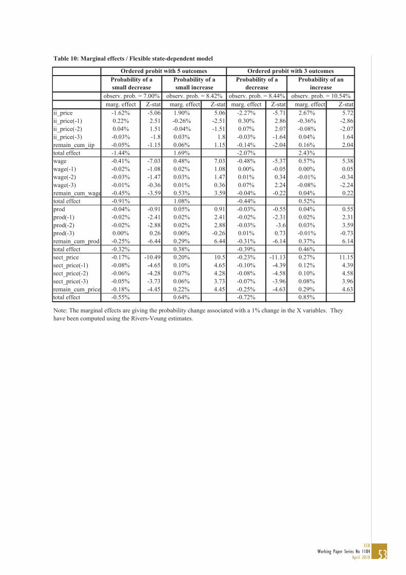
Table 10: Marginal effects / Flexible state-dependent model

marg. effect Z-stat marg. effect Z-stat marg. effect Z-stat marg. effect Z-statii_price -1.62% -5.06 1.90% 5.06 -2.27% -5.71 2.67% 5.72ii_price(-1) 0.22% 2.51 -0.26% -2.51 0.30% 2.86 -0.36% -2.86ii_price(-2) 0.04% 1.51 -0.04% -1.51 0.07% 2.07 -0.08% -2.07ii_price(-3) -0.03% -1.8 0.03% 1.8 -0.03% -1.64 0.04% 1.64remain_cum_iip -0.05% -1.15 0.06% 1.15 -0.14% -2.04 0.16% 2.04total effect -1.44% 1.69% -2.07% 2.43%wage -0.41% -7.03 0.48% 7.03 -0.48% -5.37 0.57% 5.38wage(-1) -0.02% -1.08 0.02% 1.08 0.00% -0.05 0.00% 0.05wage(-2) -0.03% -1.47 0.03% 1.47 0.01% 0.34 -0.01% -0.34wage(-3) -0.01% -0.36 0.01% 0.36 0.07% 2.24 -0.08% -2.24remain_cum_wage -0.45% -3.59 0.53% 3.59 -0.04% -0.22 0.04% 0.22total effect -0.91% 1.08% -0.44% 0.52%prod -0.04% -0.91 0.05% 0.91 -0.03% -0.55 0.04% 0.55prod(-1) -0.02% -2.41 0.02% 2.41 -0.02% -2.31 0.02% 2.31prod(-2) -0.02% -2.88 0.02% 2.88 -0.03% -3.6 0.03% 3.59prod(-3) 0.00% 0.26 0.00% -0.26 0.01% 0.73 -0.01% -0.73remain_cum_prod -0.25% -6.44 0.29% 6.44 -0.31% -6.14 0.37% 6.14total effect -0.32% 0.38% -0.39% 0.46%sect_price -0.17% -10.49 0.20% 10.5 -0.23% -11.13 0.27% 11.15sect_price(-1) -0.08% -4.65 0.10% 4.65 -0.10% -4.39 0.12% 4.39sect_price(-2) -0.06% -4.28 0.07% 4.28 -0.08% -4.58 0.10% 4.58sect_price(-3) -0.05% -3.73 0.06% 3.73 -0.07% -3.96 0.08% 3.96remain_cum_price -0.18% -4.45 0.22% 4.45 -0.25% -4.63 0.29% 4.63total effect -0.55% 0.64% -0.72% 0.85%

Note: The marginal effects are giving the probability change associated with a 1% change in the X variables. Theyhave been computed using the Rivers-Voung estimates.

observ. prob. = 7.00%

Probability of asmall increase

observ. prob. = 8.42% observ. prob. = 8.44% observ. prob. = 10.54%

Ordered probit with 5 outcomes Ordered probit with 3 outcomesProbability of a

decreaseProbability of asmall decrease

Probability of anincrease


Table 11: Estimates of a model with asymmetries

Coeff Z-stat Coeff Z-stat Coeff Z-stat Coeff Z-statii_price -0.355 -0.74 1.370 5.87 0.282 0.38 1.530 4.33ii_price(-1) 0.232 1.17 -0.271 -2.29 0.091 0.34 -0.225 -1.46ii_price(-2) 0.041 0.55 -0.046 -0.66 -0.001 -0.01 -0.025 -0.26ii_price(-3) 0.068 0.85 0.085 1.19 0.014 0.12 0.135 1.45remain_cum_iip 0.132 1.95 0.022 0.35 0.182 1.39 0.030 0.33wage 0.988 1.54 0.210 6.21 2.432 2.66 0.400 4.30wage(-1) -0.067 -2.30 0.034 2.90 -0.054 -1.07 0.006 0.23wage(-2) -0.027 -0.83 0.040 2.46 -0.071 -1.20 0.052 1.46wage(-3) -0.027 -0.62 0.035 1.17 -0.066 -1.00 0.039 0.76remain_cum_wage -0.016 -0.39 0.054 2.75 -0.240 -1.87 0.017 0.71prod 0.298 2.42 -0.223 -2.00 0.193 1.02 -0.116 -0.49prod(-1) -0.050 -1.50 0.065 3.24 -0.015 -0.28 0.070 2.00prod(-2) -0.005 -0.25 0.047 2.91 0.018 0.54 0.071 2.56prod(-3) -0.031 -1.25 0.027 1.33 -0.009 -0.27 0.022 0.66remain_cum_prod -0.100 -1.40 0.119 3.14 -0.061 -0.58 0.119 2.12sect_price 0.039 1.37 0.204 10.08 0.047 1.61 0.223 10.54sect_price(-1) 0.100 2.42 0.077 1.66 0.070 1.63 0.161 3.20sect_price(-2) -0.037 -0.77 0.221 5.15 -0.003 -0.07 0.226 5.07sect_price(-3) 0.025 0.35 0.167 2.59 0.058 0.90 0.158 2.47remain_cum_price 0.019 1.01 0.058 1.88 0.004 0.21 0.096 2.85q1 -1.971 -21.72 -1.142 -11.89q2 -1.117 -12.46q3 1.697 18.89 1.679 17.45q4 2.585 28.46LogL

Note: The estimates presented in this table are those obtained using Rivers-Vuong approach.

-33,543 -28,954



55ECB


Table 12: Marginal effects in a model with asymmetries

marg. eff. Z-stat marg. eff. Z-stat marg. eff. Z-stat marg. eff. Z-statii_price -0.38% -0.74 4.09% 5.86 0.30% 0.38 4.46% 4.33ii_price(-1) 0.16% 1.17 -0.48% -2.29 0.06% 0.34 -0.40% -1.46ii_price(-2) 0.02% 0.55 -0.07% -0.66 0.00% -0.01 -0.04% -0.26ii_price(-3) 0.03% 0.85 0.10% 1.19 0.01% 0.12 0.16% 1.45remain_cum_iip 0.27% 1.95 0.12% 0.35 0.36% 1.39 0.17% 0.33total effect 0.11% 3.76% 0.73% 4.36%wage 0.20% 1.54 0.64% 6.20 0.90% 2.66 1.24% 4.30wage(-1) -0.01% -2.30 0.08% 2.90 -0.02% -1.07 0.01% 0.23wage(-2) 0.00% -0.83 0.08% 2.46 -0.02% -1.20 0.10% 1.46wage(-3) 0.00% -0.62 0.06% 1.17 -0.02% -1.00 0.07% 0.76remain_cum_wage -0.01% -0.39 0.64% 2.75 -0.09% -1.87 0.20% 0.71total effect 0.17% 1.50% 0.77% 1.63%prod 1.36% 2.42 -1.50% -2.00 0.73% 1.02 -0.65% -0.49prod(-1) -0.18% -1.50 0.34% 3.24 -0.05% -0.28 0.31% 2.00prod(-2) -0.02% -0.25 0.21% 2.91 0.04% 0.54 0.27% 2.56prod(-3) -0.08% -1.25 0.11% 1.33 -0.02% -0.27 0.07% 0.66remain_cum_prod -0.41% -1.40 1.46% 3.14 -0.20% -0.58 1.21% 2.12total effect 0.67% 0.62% 0.50% 1.21%sect_price 0.04% 1.37 0.54% 10.01 0.06% 1.61 0.74% 10.52sect_price(-1) 0.09% 2.41 0.15% 1.66 0.08% 1.63 0.39% 3.20sect_price(-2) -0.03% -0.77 0.35% 5.14 0.00% -0.07 0.44% 5.06sect_price(-3) 0.02% 0.35 0.23% 2.59 0.05% 0.90 0.27% 2.47remain_cum_price 0.03% 1.01 0.33% 1.88 0.01% 0.21 0.69% 2.85total effect 0.15% 1.60% 0.19% 2.53%

on the prob. of a on the prob. of a on the prob. of a on the prob. of a

price decrease price increaseprice decrease price increasesmall small

obs. prob. = 8.42% obs. prob. = 8.42% obs. prob. = 10.54% obs. prob. = 10.54%



Work ing PaPer Ser i e Sno 1118 / november 2009

DiScretionary FiScal PolicieS over the cycle

neW eviDence baSeD on the eScb DiSaggregateD aPProach

by Luca Agnello and Jacopo Cimadomo

wage dynamics working paper series network … · working paper series no 1184 / april 2010 ... as...

Documents