w. t. s. f. snyder d. shipler b. j. c. - osti.gov · s. f. snyder d. shipler ... computer codes and...
TRANSCRIPT
PNWD-2227 HEDR UC-OOO
W. T. Farris B. A. Napier J. C. Simpson
S. F. Snyder D. B. Shipler
July 1994
Prepared for the Technical Steering Panel and the Centers for Disease Control and Prevention under Contract 200-92-0503(CDC)/18620(BNW)
Pacific Northwest Laboratories
. .. .” . . . L


PNWD-2227 HEDR uc-000
Columbia River Pathway Dosimetry Report, 1944-1992
Hanford Environmental Dose Reconstruction Project
W. T. Farris B. A. Napier J . C. Simpson S . F. Snyder D. B. Shipler
July 1994
Prepared for the Technical Steering Panel and the Centers for Disease Control and Prevention under Contract 200-92-0503(CDC)/ 18620Q3NW)
Battelle Pacific Northwest Laboratories Richland, Washington 99352

Columbia River Pathway Dosimetry Report, 1944-1992
July 1994
This document has been reviewed and approved by the Technical Steering Panel.
M. L. Blazek, Chair Date Technical Steering'Panel
Preface
In 1987, the U.S. Department of Energy (DOE) directed the Pacific Northwest Laboratory, whch is operated by Battelle Memorial Institute, to conduct the Hanford Environmental Dose Reconstruction (HEDR) Project. The DOE directive to begin project work followed a 1986 recommendation by the Hanford Health Effects Review Panel (HHERP). The HHERP was formed to consider the potential health implications of past releases of radioactive materials from the Hanford Site near Richland, Washington.
Members of a Technical Steering Panel (TSP) were selected to direct the HEDR Project work. The TSP consists of experts in the various technical fields relevant to HEDR Project work and representatives from the states of Washington, Oregon, and Idaho; Native American tribes; and the public. The technical members on the panel were selected by the vice presidents for research at major universities in Washington and Oregon. The state representatives were selected by the respective state governments. The Native American tribes and public representatives were selected by the other panel members.
A December 1990 Memorandum of Understanding between the Secretaries of the DOE and the U.S. Department of Health and Human Services (DHHS) transferred responsibility for managing the dose reconstruction and exposure assessment studies to the DHHS. This transfer resulted in the current contract between Battelle, Pacific Northwest Laboratories (BNW) and the Centers for Disease Control and Prevention (CDC), an agency of the DHHS.
The purpose of the HEDR Project is to estimate the radiation dose that individuals could have received as a result of radionuclide emissions since 1944 from the Hanford Site. A major objective of the HEDR Project is to determine possible radiation doses resulting from radionuclides released to the Columbia River.
The HEDR Project work is conducted under several technical and administrative tasks, among which is the Environmental Pathways and Dose Estimates Task. The staff on this task provide the computer codes and dose calculation tools required for estimating doses to individuals who may have been exposed to radioactive releases from the Hanford Site. The dose estimates are the primary objective of the project. Doses are calculated for a number of exposure pathways for the years 1944- 1992. Doses are presented for a series of locations on the Columbia River downstream from the Hanford Site. This report includes a brief description of the methods used to estimate doses to representative individuals who ingested water, fish, or waterfowl from the Columbia River or who spent time swimming in or boating on the river. The computer model, Columbia River Dosimetry (CRD), developed by BNW to estimate potential doses to representative individuals via the Columbia River will be turned over to CDC. The CRD model will be used for the Hanford Thyroid Disease Study to estimate potential doses to specific individuals.
Doses estimated for the Columbia River pathway, the subject of this report, are the result of work conducted on various technical tasks. The information necessary to estimate doses has been documented in other reports published by the HEDR Project. These reports include information on radionuclides released from Hanford reactors (Heeb and Bates 1994), transport of radionuclides in
... 111

Columbia River water (Waiters et al. 1994), accumulation of radioactivity in aquatic organisms (Thiede et al. 1994), and dose calculation methods and human exposure parameters (Snyder et al. 1994). This dosimetry report is an update of the dosimetry report published earlier (PNL 1991) but is more complete and includes additional data collected by the HEDR Project since 1991.
This report completes HEDR Project Milestone 0705B. It is the final report, replacing the previous version dated April 1994. Appendix B is a record of the TSP comments and BNW responses that have been addressed in this final report. Changes made in response to the comments are denoted by numbers in the left margin and italicized text.
iv

Summary
The purpose of the Hanford Environmental Dose Reconstruction (HEDR) Project is to estimate the radiation dose that individuals could have received as a result of radionuclide emissions since 1944 from the Hanford Site. One objective of the HEDR Project is to estimate doses to individuals who were exposed to the radionuclides released to the Columbia River (the river pathway). This report documents the last in a series of dose calculations conducted on the Columbia River pathway.
The report summarizes the technical approach used to estimate radiation doses to three classes of representative individuals who may have used the Columbia River as a source of drinking water, food, or for recreational or occupational purposes. In addition, the report briefly explains the approaches used to estimate the radioactivity released to the river, the development of the parameters used to model the uptake and movement of radioactive materials in aquatic systems such as the Columbia River, and the method of calculating the Columbia River’s transport of radioactive materials.
Potential Columbia River doses have been determined for representative individuals since the initiation of site activities in 1944. For this report, dose calculations were performed using conceptual models and computer codes developed for the purpose of estimating doses. All doses were calculated for representative individuals who share similar characteristics with segments of the general population.
Scope of Work
Doses to representative individuals from reactor releases to the Columbia River have been esti- mated and presented for the years 1944-1992. Detailed dose estimates are presented for three types of representative individuals: a maximally exposed individual (maximum representative individual). a typically exposed individual (typical representative individual), and an individual exposed on the job (occupational representative individual). Representative individuals are not intended to depict any real individual, but to share the general life-style characteristics of broad segments of the population. Representative individuals can thus provide a basis for evaluating and comparing doses to large cross- sections of the affected population.
Dose estimates were calculated for the three representative individual types in 12 segments of the Columbia River from the Hanford Site to below Portland, Oregon, and include ingestion of Willapa Bay shellfish and salmon or steelhead caught in the river. Doses were calculated for five radionuclides that together contributed over 94 percent of the total dose: sodium-24, phosphorus-32, zinc-65, arsenic-76, and neptunium-239. Doses in this report are presented as the effective dose equivalent and dose equivalent for the red bone marrow and lower large intestine.
5 The doses from 1950-1971 have been found to be the largest because of radionuclide releases during those years: thus, doses for this period are estimated with the greatest detail. provide a more complefe dose history, additional dose calculations are also presented for 1944 through 1949. Estimated doses that were previously published in Hanford annual environmental reports are summarized to complete the dose history for the years 1972 through 1992.
However. to
V

Technical Approach
Estimating doses to the representative individuals from the Columbia River pathway starts with the source term estimate; Le., an estimate of the radionuclides discharged from the eight single-pass Hanford production reactors into the Columbia River. Using information from the source term estimates, concentrations of the five key radionuclides in the Columbia River water at several down- stream locations are calculated by computer simulations of how the radionuclides flow and are trans- ported in the river. Once the radionuclide concentrations are calculated at the various locations, the effects of environmental accumulation can be determined. Dose estimates can then be made for representative individuals.
The computer codes used for the calculations simulate the reactor, the environment, and the human components. Uncertainty, sensitivity, and model validation analyses have been conducted to support the resulting estimates. The uncertainty analyses helped determine the precision with which dose estimates can be made. The sensitivity analyses have determined the panmeters and pathways with the greatest contribution to uncertainty. Model validation compares the model estimates with actual measurements of radionuclides in the environment at the time of the releases, demonstrating the degree to which the model estimates simulate the way events actually occurred.
Results
2.18 Four separate Columbia River dose assessments have been conducted during the course of the HEDR Project and are presented in PNL (1991), Walters et al. (1992), Napier (1993), and this document. All four efforts indicate that annual doses to most individuals from river pathways are less than a few millirem per year for any given year and for all locations. Only those individuals who ingested large quantities of resident Columbia River fish could have received annual doses in excess of a hundred millirem. A complete dose history for a maximum representative (Le., maximally exposed) individual at Ringold, Washington, is shown in Figure S. 1. The cumulative dose for this represen- tative individual during the 49-year period from 1944-1992 was estimated to be approximately 1500 millirem. The period, 1950-1971, accounted for most of the cumulative dose from the Columbia River pathway. For the maximum representative individual at Ringold, approximately 93 percent (1400 millirem) of the cumulative effective dose equivalent was received during this period. The cumulative dose to the maximum representative individual at Ringold for the other years ( 1944- 1949 and 1971-1992) was approximately 100 millirem.
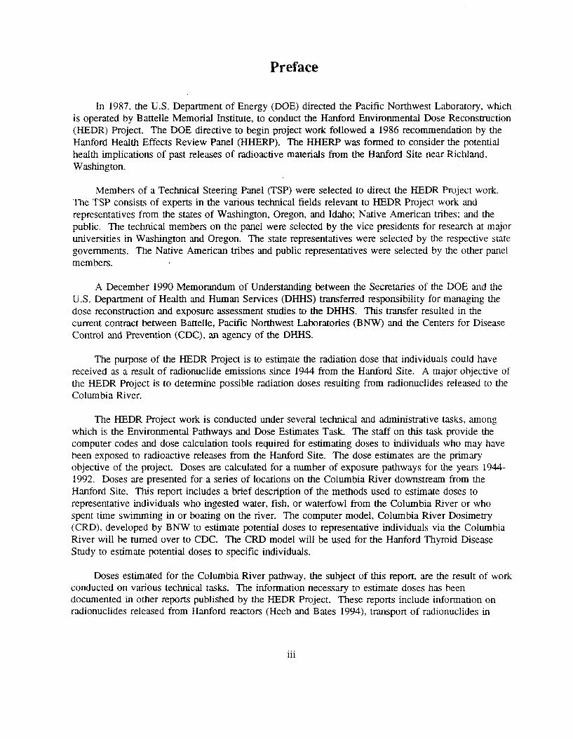
Figure S.2 shows that the doses calculated for locations near the Hanford Site (e& Ringold to Pasco) were larger than those further downriver by factors of 2 to 10, depending on the month and whether the individual was maximally exposed, typically exposed, or occupationally exposed. The decrease in dose to the downriver representative individuals was due to increased dilution and to radioactive decay of key radionuclides as they were being transported in the river. Model validation has shown that the estimated doses for the Tri-Cities area in Washington match well with the actual whole body radioactivity measurements collected during the 1960s.
vi

- Z661 - 1661 ' 0661
6861 ' 8861 r 1 L861 r 9861 [ 4861 1 P86L
t L 1861 i 0861
6L61 I 8L61 L LLGL i 9L61 ! 4L61 [ PL61
1- EL61 1- ZL6 I LL6 5- Of6 -
696 896 L96 996 496 P96 1
196 1 096 L 6S6 1 896 1 LS6 1 946 1 446 1 ~~
946 1 E46 1 246 1 1461 OS6 L 6 t 6 1 8 t 6 1 LP6 1 9 t 6 1 4P6 1
vii
/ I T I & -
~
i
//
, . >
/
/
I .
I
I ''
i I 1
4 I I
i 1 4
T I i
/
\ 0 0 0 0 0 0 0 0 0 0 0 0 0 0 0 e o 0 cv 0 m (D d cv
... VI11

Uncertainty and sensitivity analyses were conducted to estimate the range of possible doses that an individual could have received and the importance of key model parameters. For the three types of representative individuals at any location, the uncertainty range (minimum to maximum) of that person’s estimated dose is less than a factor of 10 when the diet is known. The parameters that con- tribute most to the uncertainty in the estimated dose depend upon the type of individual and exposure location. For example, the most sensitive parameters for a maximum representative individual at Richland, Washington, are the ingestion dose conversion factors (Le., the factor that translates an amount of a radionuclide ingested into an amount of radiation dose) for zinc-65 and phosphorus-32 and the holdup times (Le., time between catch and consumption) for fish caught in the river. For a typical representative individual at the same location, the uncertainty in dose is controlled by the uncertainty in the holdup time and the efficiency of the water treatment facility in removing radio- nuclides from drinking water. The uncertainty in dose estimates for locations farther downriver is controlled almost entirely by the uncertainty of the ingestion dose conversion factors.
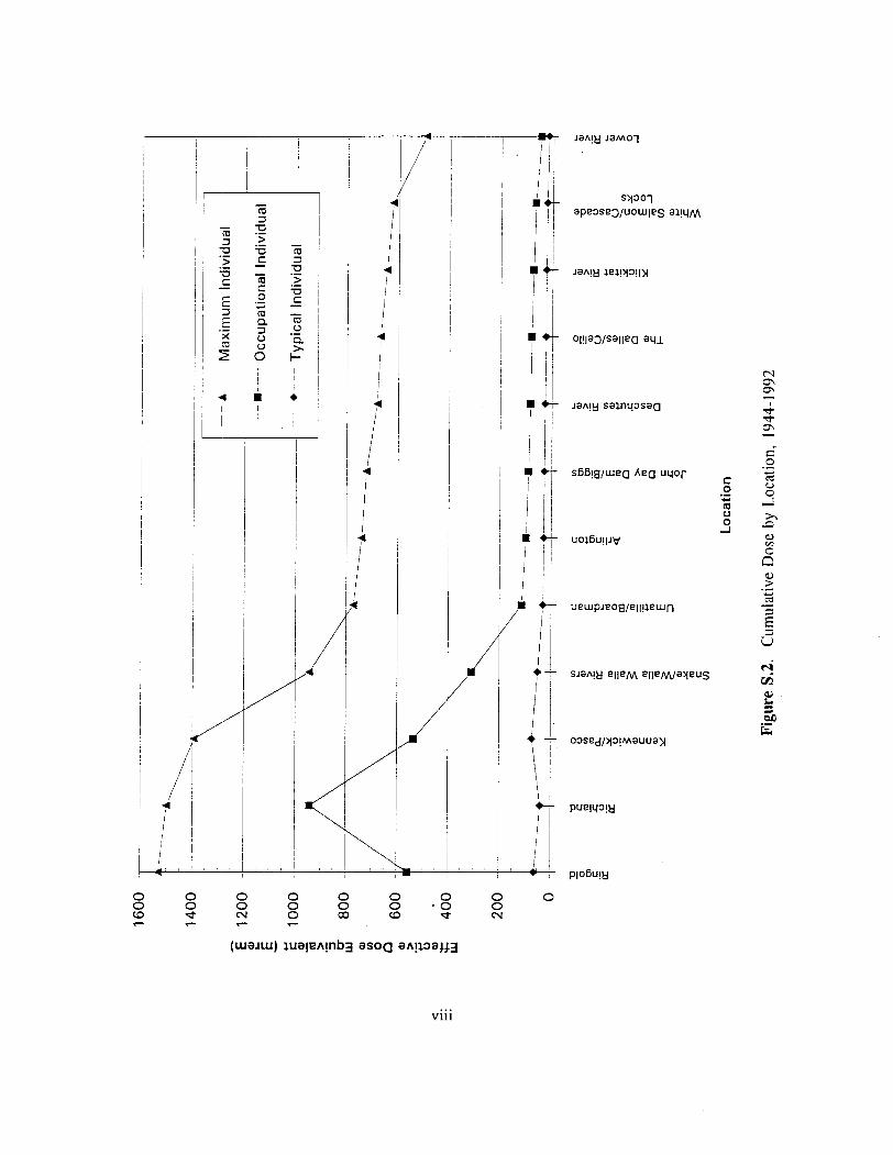
Several documents have been published by the HEDR Project that support the material presented in this report. Readers who are interested in more detail on a particular subject should consult the references listed in Table S . 1.
Conclusions
Reliable and useful doses and their uncertainties have been reconstructed for possible exposures of representative individuals from historical releases of materials from the Hanford Site.
The most important means of exposure via the river pathway was consumption of resident fish.
The most important contributors to dose were zinc45 and phosphorus-32, respectively, released from the single-pass reactors.
The highest estimated dose was from resident fish caught in the Columbia River at Ringold, Washington, downstream of the Hanford reactors.
The highest estimated dose was to an adult consuming 40 kilograms (90 pounds) of resident fish from the Columbia River at Ringold, Washington (median dose of 140 millirem to the whole body for 1960).
The highest estimated dose to a typical adult was accumulated during the 1956-1965 time period with 1960 being the highest year (median dose of 5 millirem) at Pasco, Washington.
Doses for children for any specific year could be a factor of 1.5 to 2 higher than the adult doses for the typical representative individual.
The most important contributors to uncertainty in the dose estimates were the dose factor and the bioconcentration factors, respectively.
Representative individual doses included in this report allow individuals using the Columbia
ix
Table S.1. Key Sources of Information for the Columbia River Pathway
11 Type of Information
General Project Planning
Radionuclide Releases to the Columbia River
Radionuclide Transport in the Columbia River
Environmental Historical Measurements Related to the Columbia River
/I Methodology for Calculating Doses
HEDR Project Document
Shipler, D.B. 1993. Integrated Task Plans for the Hanford Dose Reconstruction Project, June I992 Through May 1994. PNWD-2 187 HEDR, Battelle, Pacific Northwest Laboratories, Richland, Washington.
Heeb, C.M., and D.J. Bates. 1994. Radionuclide Releases to the Columbia River from Hanford Operations, 1944-1 971. PNWD-2223 HEDR, Battelle, Pacific Northwest Laboratories, Richland, Washington.
Walters, W.H., M.C. Richmond, and B.G. Gilmore. 1994. Reconstruction of Radionuclide Concentrations in the Columbia River from Hanford, Washington, to Portland, Oregon, January 1950-January 1971. PNWD-2225 HEDR, Battelle, Pacific Northwest Laboratories, Richland, Washington.
Thiede, ME. , D.J. Bates, E.I. Mart, and R.W. Hanf. 1994. A Guide to Environmental Monitoring Data, 1945 through 1972. PNWD-2226 HEDR, Battelle, Pacific Northwest Laboratories, Richland. Washington.
Denham, D.H., R.L. Dikes, R.W. Hanf, T.M. Poston, M.E. Thiede, and R.K. Woodruff. 1993. Phase I Summaries of Radionuclide Concentration Data for Vegetation, River Water, Drinking Water, and Fish. PNWD-2 145 HEDR, Battelle, Pacific Northwest Laboratories, Richland, Washington.
Walters, W.H., R.L. Dirkes, and B.A. Napier. 1992. Literature and Data Review for the Surface-Water Pathway: Columbia River and Adjacent Coastal Areas. PNWD-2034 HEDR, Battelle, Pacific Northwest Laboratories, Richland, Washington.
Shipler, D.B., and B.A. Napier. 1994. HEDR Modeling Approach. PNWD-1983 HEDR Rev. 1 , Battelle, Pacific Northwest Laboratories, Richland, Washington.
X

Table S.1. (contd)
11 Type of Information
Equations and Panmeter Values Used in Environmental Accumulation and Dose Calculations
Methods for Conducting Model Uncertainty and Sensitivity Analyses
Previous HEDR Dose Estimates for the Columbia River Pathway
Validation of HEDR Models I
HEDR Project Document
Snyder, S.F., W.T. Fams, B.A. Napier, T.A. Ikenberry, and R.O. Gilbert. 1994. Parameters Used in the Environmental Pathways and Radiological Dose Modules (DESCARTES, CIDER, and CRD Codes) of the Hanford Environmental Dose Reconstruction Integrated Codes (HEDRX). PNWD-2023 HEDR Rev. 1, Battelle, Pacific Northwest Laboratories, Richland, Washington.
Simpson, J.C., and J.V. Ramsdell, Jr. 1993. Uncertainty and Sensitivity Analyses Plan. PNWD-2 124 HEDR, Battelle, Pacific Northwest Laboratories, Richland, Washington.
Napier, B.A. 1993. Determination of Key Radionuclides and Parameters Related to Dose from the Columbia River Pathway. BN-SA-3768 HEDR, Battelle, Pacific Northwest Laboratories, Richland, Washington.
Walters, W.H., R.L. Dirkes, and B.A. Napier. 1992. Literature and Data Review for the Sulface- Water Pathway: Columbia River and Adjacent Coastal Areas. PNWD-2034 HEDR, Battelle, Pacific Northwest Laboratories, Richland, Washington.
PNL - Pacific Northwest Laboratory. 199 1. Columbia River Pathway Report: Phase I of the Hanford Environmental Dose Reconstruction Project. PNL-74 1 1 HEDR Rev. 1, Pacific Northwest Laboratory, Richland. Washington.
Napier, B.A., J.C. Simpson, P.W. Eslinger, J.V. Ramsdell, Jr., M.E. Thiede, and W.H. Walters. 1994. Validation of HEDR Models. PNWD-222 1 HEDR, Battelle, Pacific Northwest Laboratones, Richland, Washington.
xi

Glossary
anadromous - fish that live part of their lives in fresh water and part in salt water. living in the ocean, spawning in fresh water.
bioconcentration factor - ratio between the radionuclide concentration in biota to the radionuclide concentration in the water in whch they live and feed.
biota - plants and animals.
body burden - amount of a given radionuclide in humans, typically measured in nanocuries.
boxplot - graphical representation of the distribution of values in which a box shows the middle 50 percent of the distribution and the "whiskers" indicate the lower and upper 5 percent of the distribution.
CHARIMA - CHArriage des RIvieres MAillees, computer code that models sediment transport in multiple channel river systems.
Ci - abbreviation for curie.
code - computer implementation of equations. Codes can also retrieve, manipulate, display, store data, etc.
composite sample - sample composed of small portions collected from several locations or from ;I single location over an extended time period.
concentration - amount of a specified substance (e,g., a radioactive element) in a unit amount of another substance (e.& river water).
CRD - Columbia River Dosimetry, computer code used to estimate doses to real individuals.
curie - unit of radioactivity corresponding to 3.7 x 10" (37 billion) disintegrations per second (abbreviated Ci).
deterministic - estimation method where a single-point estimate is calculated (contrast with "stochastic").
dose - radiation dose; often distinguished as absorbed dose, dose equivalent, or effective dose equivalent.
absorbed dose - amount of energy deposited by radiation in a given amount of material, such as tissue; measured in rad.
... X l l l

7
dose equivalent - quantity calculated to compare relative biological effectiveness of different kinds of radiation, using a common numerical scale; determined by multiplying absorbed dose by a quality factor and other modifying factors; measured in rem (a millirem is one-thousandth of a rem).
effective dose equivalent (EDE) - value used to account for the fact that a rem of radiation to one organ in the body does not have the same potential health impact as a rem of dose to another organ. I t is the sum of the dose to all organs of the body from internal deposition of radionuclides and the dose from external radiation exposure; measured in rem.
dose factor - factor that describes the amount of radiation dose received from a given intake of radioactivity.
effluent plume - spread of contaminants in air, surface water, or ground water released from a contaminant source.
empirical - results obtained by relying on observation or experiment.
first-order predator - fish that consume other fish; includes perch, crappie, punkinseed, and bluegill.
fuel element - aluminum-clad rod used in Hanford reactors.
fuel-element failure - rupture of a fuel element, leading to an usually high radioactive contamination of the cooling water.
grab sample - sample collected from a single location at a specific time.
gross beta - total activity of beta-emitting radionuclides that could not be distinguished separately by ins tnun e n ta ti o n .
half-life - time required for an initial number of radioactive atoms to be reduced to half that number by transformations.
histogram - bar graph of a frequency distribution in which the widths of the bars are proportional to the classes into which the variable has been divided and the heights of the bars are proportional to the class frequencies.
isotope - one of two or more atoms having the same atomic number but different mass.
LLI - lower large intestine.
mean - avenge value of a set of numbers.
median - middle value in a series of values arranged in order of size.
model - conceptual representation of physicalhiological processes. The representation may be c graphical or a set of mathematical equations that simulate the process being modeled.
xi v

modules - sections of a computer code.
Monte Carlo technique - method that represents the effect of uncertainty in one or more contributing parameters on the overall uncertainty by randomly sampling distribution functions whch express parameter uncertainty.
m a d - millirad, one-thousandth of a rad.
mrem - millirem, one-thousandth of a rem.
8 neutron flux - rate of neutron bombardment passing through a unit cross-sectional area.
omnivore - fish that eat both plants and animals; includes bullheads, catfish, suckers, whtefish, chiselmouth, chub, sturgeon, minnows, and shiners.
picocurie - one-trillionth of a curie.
process tube - aluminum tube that held the uranium fuel elements and cooling water in Hanford reactors.
rad - radiation absorbed dose, unit of measurement used to describe absorbed dose.
radioactive decay - emission of radiation, such as alpha, beta, or gamma rays from unstable isotopes of an element.
radionuclide - isotope of an element that exhibits radioactivity.
RBM - red bone mmow.
realization - particular pass through a Monte Carlo simulation in which all stochastic parameters have been assigned a value; the simulation represents a "possible reality."
rem - roentgen equivalent man, unit of measurement used to describe dose equivalent.
representative individuals - hypothetical individuals sharing similar characteristics significant for estimating dose; in this report, three types of representative individuals are defined: maximum, occupational, and typical.
maximum representative individual - significant user of the Columbia River who spent time in or on the river and ingested maximum or near maximum amounts of fish and waterfowl.
occupational representative individual - individual who was exposed to the Columbia River only in the course of work (such as commercialfishemen or boat operators) and ingested no resident fish or shellfish.
xv

typical representative individual - individual residing near the Columbia River who ingested river water but no resident fish or waterfowl.
second-order predator - predatory fish that consume other predatory fish; includes bass, trout, and squawfish.
sensitivity - determination of the parameters and pathways that contribute most to uncertainty in dose results.
single-pass reactors - plutonium production reactors (B, C, D, DR, F, H, KE, KW reactors) that did not recirculate Columbia River water but instead discharged it into retention basins and, after a hold up time, into the Columbia River.
source term - amount of radioactivity (curies) of a radionuclide released to the environment from a facility at a given time.
stochastic - method of estimating possible values that incorporate the variability in input parameters to arrive at a corresponding set of possible results (contrast with "deterministic").
STRRM - Source Term River Release Model, computer code that provides estimates of monthly releases of radionuclides from Hanford reactors to the Columbia River.
transmission factor - amount of radioactivity that remains after municipal water treatment.
uncertainty - measure of variability in model parameters or dose estimates.
validation - model validation, comparison of estimated values to historical measurements as a test of the reliability of the model estimates.
WSU-CHARIMA - Washington State University modified CHARMA computer code; modification allowed for radionuclide decay.
xv i

Contents
... Preface . . . . . . . . . . . . . . . . . . . . . . . . . . . . . . . . . . . . . . . . . . . . . . . . . . . . . . . . . . . . . 111
summary . . . . . . . . . . . . . . . . . . . . . . . . . . . . . . . . . . . . . . . . . . . . . . . . . . . . . . . . . . . V
... Glossary . . . . . . . . . . . . . . . . . . . . . . . . . . . . . . . . . . . . . . . . . . . . . . . . . . . . . . . . . . . . xiii
1.0 Introduction . . . . . . . . . . . . . . . . . . . . . . . . . . . . . . . . . . . . . . . . . . . . . . . . . . . . . . 1.1
1.1 Purpose . . . . . . . . . . . . . . . . . . . . . . . . . . . . . . . . . . . . . . . . . . . . . . . . . . . . . . 1.1
1.2 Scope . . . . . . . . . . . . . . . . . . . . . . . . . . . . . . . . . . . . . . . . . . . . . . . . . . . . . . . 1.2
1.3 Preview of Report . . . . . . . . . . . . . . . . . . . . . . . . . . . . . . . . . . . . . . . . . . . . . . 1.2
2.0 Data Quality Objectives . . . . . . . . . . . . . . . . . . . . . . . . . . . . . . . . . . . . . . . . . . . . . . 2.1
2.1 Accuracy . . . . . . . . . . . . . . . . . . . . . . . . . . . . . . . . . . . . . . . . . . . . . . . . . . . . . 2.1
2.2 Precision . . . . . . . . . . . . . . . . . . . . . . . . . . . . . . . . . . . . . . . . . . . . . . . . . . . . . 2.1
2.3 Completeness . . . . . . . . . . . . . . . . . . . . . . . . . . . . . . . . . . . . . . . . . . . . . . . . . . 2.1
2.4 Representativeness . . . . . . . . . . . . . . . . . . . . . . . . . . . . . . . . . . . . . . . . . . . . . . 2.2
2.5 comparability . . . . . . . . . . . . . . . . . . . . . . . . . . . . . . . . . . . . . . . . . . . . . . . . . 2.2
3.0 Technical Approach . . . . . . . . . . . . . . . . . . . . . . . . . . . . . . . . . . . . . . . . . . . . . . . . 3 . I
3.1 Source Term Model . . . . . . . . . . . . . . . . . . . . . . . . . . . . . . . . . . . . . . . . . . . . . 3.4
3.1.1 Mechanism for Source Term Releases to River . . . . . . . . . . . . . . . . . . . . . 3.5
3.1.2 Radionuclide Release Estimates . . . . . . . . . . . . . . . . . . . . . . . . . . . . . . . . 3.6
3.2 River Transport Model . . . . . . . . . . . . . . . . . . . . . . . . . . . . . . . . . . . . . . . . . . . 3.6
3.8 3.2.1 Development of the Columbia River Transport Conceptual Model . . . . . . . .
3.2.2 Model Validation . . . . . . . . . . . . . . . . . . . . . . . . . . . . . . . . . . . . . . . . . . 3.10
3.2.3 Columbia River Modeling Results . . . . . . . . . . . . . . . . . . . . . . . . . . . . . . 3.11
xvii
3.3 Radionuclide Concentrations in Aquatic Organisms . . . . . . . . . . . . . . . . . . . . . . . 3.13
3.3.1 Fish and Waterfowl Bioconcentradon Factors . . . . . . . . . . . . . . . . . . . . . . 3.13
3.3.2 Willapa Bay Shellfish Data . . . . . . . . . . . . . . . . . . . . . . . . . . . . . . . . . . . 3.16
3.3.3 Salmon Data . . . . . . . . . . . . . . . . . . . . . . . . . . . . . . . . . . . . . . . . . . . . . 3.18
3.4 Dose Assessment . . . . . . . . . . . . . . . . . . . . . . . . . . . . . . . . . . . . . . . . . . . . . . . 3.20
3.4.1 Capabilities of the Columbia River Dosimetry Code . . . . . . . . . . . . . . . . . . 3.20
3.4.2 Equations in the Columbia River Dosimetry Code . . . . . . . . . . . . . . . . . . . 3.21
3.4.3 Representative Individual Definitions . . . . . . . . . . . . . . . . . . . . . . . . . . . . 3.25
4.0 Results . . . . . . . . . . . . . . . . . . . . . . . . . . . . . . . . . . . . . . . . . . . . . . . . . . . . . . . . . . 4.1
4.1 Annual Doses, 1944-1992 . . . . . . . . . . . . . . . . . . . . . . . . . . . . . . . . . . . . . . . . . 4.1
4.1.1 Radionuclides Contributing to Dose . . . . . . . . . . . . . . . . . . . . . . . . . . . . . 4.2
4.1.2 Screening Dose Calculations, 1944-1949 . . . . . . . . . . . . . . . . . . . . . . . . . . 4.3
4.1.3 Detailed Dose Calculations, January 1950-January 1971 . . . . . . . . . . . . . . . 4.3
4.1.4 Doses from Hanford Annual Reports, 1971-1992 . . . . . . . . . . . . . . . . . . . . 4.4
4.1.5 Complete Dose History . . . . . . . . . . . . . . . . . . . . . . . . . . . . . . . . . . . . . . 4.8
4.1.6 Comparison to Feasibility Study Dose Estimates . . . . . . . . . . . . . . . . . . . . 4.8
4.2 Key Exposure Pathways and Radionuclides . . . . . . . . . . . . . . . . . . . . . . . . . . . . . 4.12
4.3 Doses from Ingestion of Salmon and Steelhead . . . . . . . . . . . . . . . . . . . . . . . . . . 4.16
4.4 Dose from Ingestion of Shellfish . . . . . . . . . . . . . . . . . . . . . . . . . . . . . . . . . . . . 4.21
5.0 Model Reliability . . . . . . . . . . . . . . . . . . . . . . . . . . . . . . . . . . . . . . . . . . . . . . . . . . 5.1
5.1 Uncertainty and Sensitivity Analyses . . . . . . . . . . . . . . . . . . . . . . . . . . . . . . . . . 5.1
5.1.1 Analysis Techniques . . . . . . . . . . . . . . . . . . . . . . . . . . . . . . . . . . . . . . . . 5.2
5.1.2 Uncertainties in Dose Estimates . . . . . . . . . . . . . . . . . . . . . . . . . . . . . . . . 5.2
5.1.3 Key Model Parameters . . . . . . . . . . . . . . . . . . . . . . . . . . . . . . . . . . . . . . 5.10
xviii

5.2 Model Validation . . . . . . . . . . . . . . . . . . . . . . . . . . . . . . . . . . . . . . . . . . 5.13
5.2.1 Validation of Dose Model Inputs . . . . . . . . . . . . . . . . . . . . . . . . .
5.2.2 Validation of Reference Individual Doses . . . . . . . . . . . . . . . . . . . .
5.13
5.17
5.2.3 Validation of Real Individual Doses . . . . . . . . . . . . . . . . . . . . . . . . . . 5.17
6.0 Conclusions . . . . . . . . . . . . . . . . . . . . . . . . . . . . . . . . . . . . . . . . . . . . . . . . . 6.1
7.0 References . . . . . . . . . . . . . . . . . . . . . . . . . . . . . . . . . . . . . . . . . . . . . . . . . 7.1
Appendix A . Summary of Estimated Columbia River Doses . . . . . . . . . . . . . . . . . . . . . A . 1
Appendix B . Summary of Technical Steering Panel Comments and Battelle. Pacific Northwest Laboratories Responses . . . . . . . . . . . . . . . B.1
xix
Figures
s . 1
s . 2
3.1
3.2
3.3
3.4
3.5
3.6
3.7
3.8
4.1
4.2
4.3
4.4
4.5
4.6
4.7
Dose History for a Maximum Representative Individual at Ringold. Washington. 1944- 1992 . . . . . . . . . . . . . . . . . . . . . . . . . . . . . . . . . . . . . . vii
Cumulative Dose by Location. 1944- 1992 . . . . . . . . . . . . . . . . . . . . . . . . . . . . . . . viii
Columbia River Pathway Integrated Codes . . . . . . . . . . . . . . . . . . . . . . . . . . . . . . . 3.2
Key Radionuclides Released to the Columbia River by Year. 1944-1971 . . . . . . . . . . 3.7
River/Ocean Radionuclide Burden. 1944- 197 1 . . . . . . . . . . . . . . . . . . . . . . . . . . . . 3.7
Columbia River Pathway Model Study Area . . . . . . . . . . . . . . . . . . . . . . . . . . . . . . 3.9
Comparison of Estimated versus Measured Radioactivity in Columbia River Water at Richland. Washington . . . . . . . . . . . . . . . . . . . . . . . . . . . . . . . . . . . . . . . 3.11
Estimated Radionuclide Concentrations in Columbia River Water at Richland. Washington. 1956-1965 . . . . . . . . . . . . . . . . . . . . . . . . . . . . . . . . . . . . . . . . . . . . 3.12
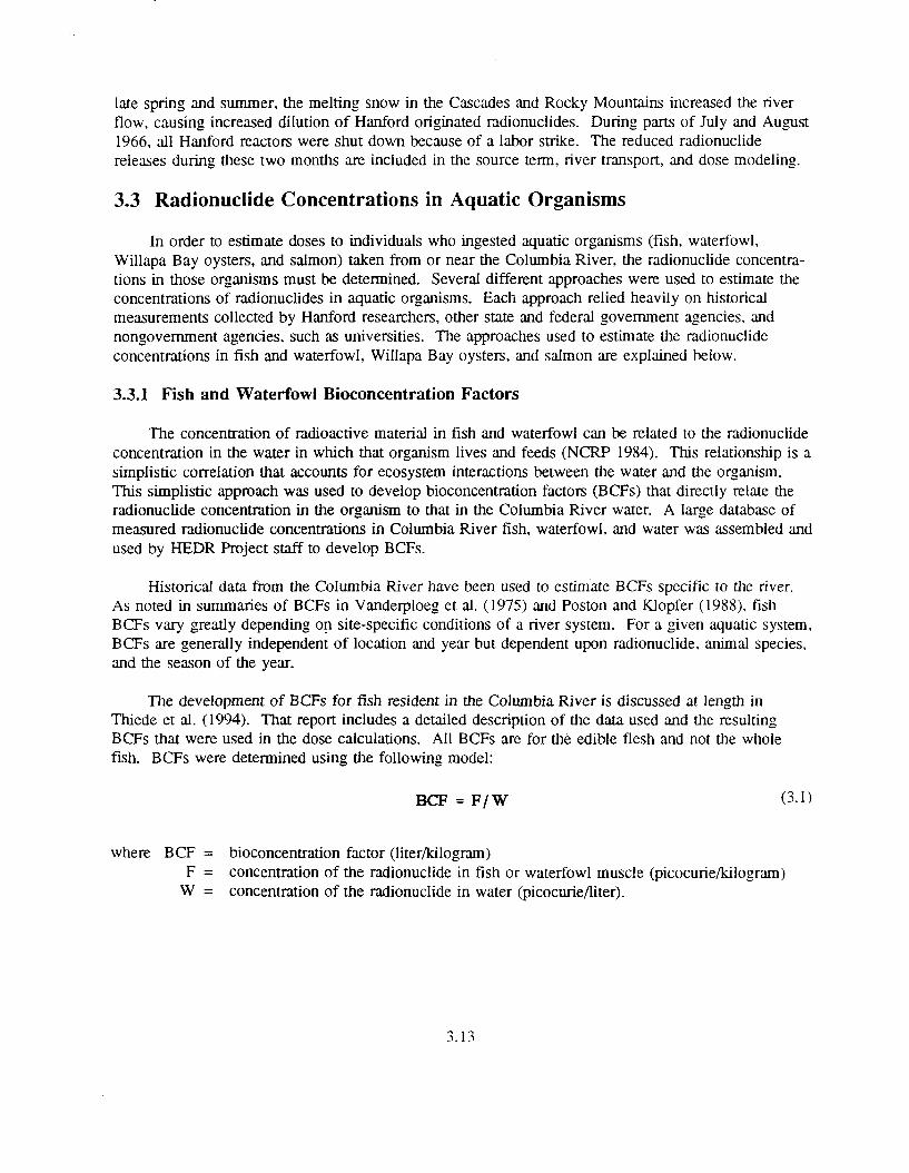
Estimated Zinc-65 Concentrations in Aquatic Organisms at Richland. Washington. 1956-1964 . . . . . . . . . . . . . . . . . . . . . . . . . . . . . . . . . . . . . . . . . . . . 3.17
Zinc-65 Concentrations in Salmon at Ringold. Washington. 1950-1971 . . . . . . . . . . . 3.19
Contribution to Total Effective Dose Equivalent for a Maximum Representative Individual at Richland. Washington. 1944-1971 . . . . . . . . . . . . . . . . . . . . . . . . . . . . 4.2
Annual Doses to a Maximum Representative Individual at Selected Columbia River Locations. 1950-1970 . . . . . . . . . . . . . . . . . . . . . . . . . . . . . . . . . . 4.5
Annual Doses to a Typical Representative Individual at Selected Columbia River Locations. 1950- 1970 . . . . . . . . . . . . . . . . . . . . . . . . . . . . . . . . . . 4.6
Annual Doses to an Occupational Representative Individual at Selected Columbia River Locations. 1950-1970 . . . . . . . . . . . . . . . . . . . . . . . . . . . . . . . . . . 4.7
Dose History for a Maximum Representative Individual at Ringold. Washington. 1944-1992 . . . . . . . . . . . . . . . . . . . . . . . . . . . . . . . . . . . . . . 4 1 . I
Comparison to Feasibility Study Doses. 1964-1966 . . . . . . . . . . . . . . . . . . . . . . . . . 4.12
Dose from Consumption of Salmon or Steelhead with 1 Picocurie of Zinc-65 per Gram . . . . . . . . . . . . . . . . . . . . . . . . . . . . . . . . . . . . . . . . . . . . . . . . 4.18
xx

4.8
5.1
5.2
5.3
5.4
5.5
5.6
5.7
5.8
5.9
5.10
5.11
5.12
5.13
Dose from Consumption of 100 Kilograms per Year of Salmon or Steelhead at Selected Locations. 1950- 1970 . . . . . . . . . . . . . . . . . . . . . . . . . . . . . . . . . . . . . . . 4.20
Example of a Boxplot Used to Display Uncertainty Ranges for Dose Estimates . . . . . 5.3
Uncertainty in Effective Dose Equivalent for Two Types of Individuals at Richland. Washington and The Dalles. Oregon. 1950-1971 . . . . . . . . . . . . . . . . . . 5.5
Uncertainty in Dose Equivalent to Lower Large Intestine for Two Types of Individuals at Richland. Washington. and The Dalles. Oregon. 1950-1971 . . . . . . . . . 5.6
Uncertainty in Dose Equivalent to Red Bone Marrow for Two Types of Individuals at Richland. Washington. and The Dalles. Oregon. 1950-1971 . . . . . . . . . . . . . . . . . 5.7
Uncertainty in Pathway Contribution to Effective Dose Equivalent for a Maximum Representative Individual at Richland. Washington. 1950-1971 . . . . . . . . . 5.8
Uncertainty in Pathway Contributions to Effective Dose Equivalent for a Maximum Representative Individual at The Dalles. Oregon. 1950- 197 1 . . . . . . . . . . . 5.9
Parameters Contributing to Uncertainty of Dose to a Maximum Representative Individual in Richland. Washington . . . . . . . . . . . . . . . . . . . . . . . . . . . . . . . . . . . . 5.11
Panmeters Contributing to Uncertainty in Total Effective Dose Equivalent . . . . . . . . 5.12
Parameters Contributing to Uncertainty in Dose Equivalent to Lower Large Intestine . . . . . . . . . . . . . . . . . . . . . . . . . . . . . . . . . . . . . . . . . . . 5.14
Parameters Contributing to Uncertainty in Dose Equivalent toRed BoneMarrow . . . . . . . . . . . . . . . . . . . . . . . . . . . . . . . . . . . . . . . . . . . . . . 5.15
Sodium-24 Comparison of Whole Body Counts and Model Estimates . . . . . . . . . . . . 5.18
Zinc-65 Comparison of Whole Body Counts and Model Estimates . . . . . . . . . . . . . . 5.19
Estimated and Measured Zinc-65 Body Burden . . . . . . . . . . . . . . . . . . . . . . . . . . . . 5.20
xxi

s . 1
3.1
3.2
3.3
3.4
3.5
3.6
3.7
4.1
4.2
4.3
4.4
4.5
4.6
A . 1
A.2
A.3
A.4
A.5
A.6
X Key Sources of Information for the Columbia River Pathway . . . . . . . . . . . . . . . . . .
Median Bioconcentration Factors for Columbia River Fish Using Historical Fish Measurements and WSU-CHARIMA Estimated Water Concentrations . . . . . . . . 3.15
Median Bioconcentration Factors for Columbia River Waterfowl . . . . . . . . . . . . . . . 3.16
Transmission Factors for Five Key Radionuclides . . . . . . . . . . . . . . . . . . . . . . . . . . 3.23
Characteristics of the Maximum Representative Individual . . . . . . . . . . . . . . . . . . . .
Characteristics of the Typical Representative Individual . . . . . . . . . . . . . . . . . . . . . .
3.26
3.27
Characteristics of the Occupational Representative Individual . . . . . . . . . . . . . . . . . .
Holdup Times for Various Food Types . . . . . . . . . . . . . . . . . . . . . . . . . . . . . . . . . 3.29
3.28
Doses to a Maximum Representative Individual at Ringold. Washington. 1944- 1949. from Ingestion of Fish . . . . . . . . . . . . . . . . . . . . . . . . . . . . . . . . . . . . . 4.3
Hanford Annual Report Doses. 197 1-1992 . . . . . . . . . . . . . . . . . . . . . . . . . . . . . . . 4.9
Estimated Effective Dose Equivalent to a Maximum Representative Individual in Ringold. Washington . . . . . . . . . . . . . . . . . . . . . . . . . . . . . . . . . . . . . 4.10
Pathways and Radionuclides Contributing to Dose. 1956-1965 . . . . . . . . . . . . . . . . . 4.13
Annual Dose from Consumption of Salmon or Steelhead at Ringold . . . . . . . . . . . . . 4.19
Annual Dose from Consumption of Willapa Bay Oysters . . . . . . . . . . . . . . . . . . . . . 4.21
Maximum Representative Individual . Effective Dose Equivalent . . . . . . . . . . . . . . . A.2
Maximum Representative Individual . Red Bone Marrow Equivalent Dose . . . . . . . . . A.8
Maximum Representative Individual . Lower Large Intestine Equivalent Dose
Typical Representative Individual . Effective Dose Equivalent
. . . . . . A.9
A . 10 . . . . . . . . . . . . . . . . .
Typical Representative Individual . Red Bone Marrow Equivalent Dose . . . . . . . . . .
Typical Representative Individual . Lower Large Intestine Equivalent Dose . . . . . . . .
A.16
A . 17
xxii

A . 7
A . 8
Occupational Representative Individual . Effective Dose Equivalent . . . . . . . . . . . . .
Occupational Representative Individual . Red Bone Marrow Equivalent Dose . . . . . . .
A.9 Occupational Representative Individual . Lower Large Intestine Equivalent Dose . . . . A.25
A . 18
A.24
xxiii

1.0 Introduction
The Hanford Site in southeastem Washington State was selected in 1943 ;is the location for the facilities used to produce plutonium for atomic bombs during World War 11. Three plutonium produc- tion reactors (B, D, and F') began operating in 1944 and 1945. These reactors withdrew water from the Columbia River and, after extensive treatment, used that water to cool the core of the reactors. This water was first discharged to retention basins and then, after a holdup time, discharged directly to the Columbia River. These reactors were called "single-pass'' reactors because they discharged cooling water directly to the river rather than recirculating it. After the end of World War I1 in 1945, the reactors continued to be used to produce plutonium. From 1949 through 1963, six new reactors (H, DR, C, KW, E, and N) began operating. The N Reactor differed in design from the earlier reactors in that cooling water was recirculated through the reactor core instead of being discharged directly to the Columbia River. Radionuclide emissions from the N Reactor were not studied as part of this effort. However, doses from the N Reactor are included in the dose estimates presented in this report.
The availability of relatively pure Columbia River water for cooling was one of the reasons for locating plutonium production at the Hanford Site (Groves 1962). The use of river water to cool the reactors resulted in the release of radionuclides to the Columbia River. Releases of radionuclides to the ground from nuclear facilities in the Hanford 200 East and West areas resulted in smaller releases to the Columbia River (Freshley and Thome 1992). The B Reactor was shut down by 1968. By January 1971, all of the other single-pass reacton had been shut down as well, leaving the N Reactor the only plutonium-production reactor operating at the Hanford Site. The N Reactor was shut down in 1987.
Individuals who drank water from the Columbia River, ate food affected by the river. or used the river for recreational or occupational purposes would have received a radiation dose from Hanford emissions. The magnitude of that dose depends on the mount of individual use of the river and on the particular year that use occurred. Doses may have also been received by individuals who did not directly access the Columbia River. Some dose could have been acquired by the ingestion of salmon, whose migration route was the Columbia River but which were caught in the Pacific Ocean, and the ingestion of oysters from Pacific Ocean estuaries near the Columbia River.
A feasibility study for the Columbia River pathway was conducted in 1991 to determine if a retrospective assessment of the Columbia River pathway was possible and to determine the magnitude of possible radiation doses. The scope of the feasibility study was narrow and included limited time periods and locations. The general findings of the feasibility study were that sufficient historical infor- mation could be retrieved and reconstructed, computer models for dose assessment could be developed, and the modeling approach could produce credible dose estimates (PNL 1991).
1.1 Purpose
The purpose of the Hanford Environmental Dose Reconstruction (HEDR) Project is to estimate the radiation dose that representative individuals could have received as a result of radionuclide emis- sions since 1944 from the Hanford Site. This dose assessment effort expands and refines the modeling
1.1

approach used in the feasibility study dose assessment (PNL 1991). The time period covered in the feasibility study was expanded from 1964-1966 to 1944-1992 in this study. The number of feasibility study locations covered was also expanded from 5 locations between the reactors and McNary Dam to 12 locations from the reactor areas to near the mouth of the Columbia River. In addition to expanding the time periods and locations, several refinements were made to the feasibility study approach. These refinements were recommended by the HEDR Technical Steering Panel (TSP) and include a more detailed estimate of radionuclide releases from the reactors, an enhanced river transport assessment, and 3 more complete collection of historical measurements.(a) In genenl, no changes were made to the fundamental methods used to estimate the feasibility study doses.
1.2 Scope
This report estimates the doses that could have been received by three types of representative individuals as a result of radionuclide releases from Hanford production reacton to the Columbia River from 1944-1992: maximally exposed individual (referred to in the report as a maximum represen- tative individual), a typically exposed individual (typical representative individual). and an occu- pationally exposed individual who was not a worker at the Hanford Site (occupational representative individual). Detailed dose estimates for five radionuclides (sodium-24, phosphorus-32, zinc-65, arsenk-76, and neptunium-239) for the time period of largest releases (1950-1971) were estimated on a monthly basis for the three types of representative individuals. The dose estimates are based on radionuclide concentrations in 12 distinct segments of the Columbia River and include ingestion of Willapa Bay shellfish and salmon and steelhead from anywhere in the river. Radiation doses were much lower during 1944-1949 and 1972-1992. In order to show relative dose, this report provides annual doses for a maximum representative individual at the highest impact location during these years.
1.3 Preview of Report
Section 2.0 summarizes the data quality objectives for estimating radiation doses. Section 3.0 describes the technical approach used in calculating the dose to individuals from the Columbia River pathway. This section includes a discussion of the source term, river transport, environmental accumu- lation. and dose assessment procedures. The equations used to estimate dose are also presented in this section. Sample doses for 1944-1992 are presented and discussed in Section 4.0. Section 5.0 includes a discussion of model reliability, including parameter uncertainty and sensitivity analysis and vali- dation studies of the models. Conclusions are presented in Section 6.0. A detailed table showing doses to representative individuals for January 1950 through January 1971 is included in Appendix A.
(a) Memorandum (HEDR Project Document No. 11920015), "Recommendations for Further River Pathway Work, FY93." from P.C. f ingeman (TSP) to TSP Members and D.B. Shipler (BNW), September 28. 1992.
1.2

2.0 Data Quality Objectives
The data quality objectives (DQOs) for estimating radiation doses from the Columbia k v e r path- way are defined in Shipler (1993). The doses calculated and presented in this document are based on the data provided by other tasks and subtasks in the HEDR Project. The DQOs developed by other tasks bear on the overall quality of the estimated dose. The DQOs for the other HEDR tasks are also presented in Shipler (1993).
2.1 Accuracy
The accuracy objective is to estimate doses using models that have been evaluated and refined by validation studies and sensitivity/uncertainty analyses. Doses presented in this document have been estimated by using models and derived computer codes that have been tested for numerical accuracy as well as for their ability to generate results that compare with historical measurements. The validation of all the HEDR models is documented in Napier et al. (1994). That report states that, in general, the comparisons show relative agreement and that most of the calculated results show order-of-magnitude agreement with the historical measurements. The final determination of accuracy has been made by HEDR Project and TSP review of this report and of Napier et al. (1994). Uncertainty and sensitivity analyses were conducted to estimate the range of possible doses and to determine those parameters that contribute most to the uncertainty in doses.
2.2 Precision
The precision objective is to quantify the precision of dose estimates for a real individual by con- ducting uncertainty analyses using estimated parameter uncertainties and appropriate error propagation procedures. The uncertainty analyses were conducted using random-sampling techniques that have been approved by the TSP. The results of the analyses are presented in Section 5.0 of th~s report. The final determination of precision has been made by project and TSP review of this report.
2.3 Completeness
The HEDR modeling approach, developed by Shipler and Napier (1994), was used to estimate doses based on the quality and abundance of historical data available for source term and environ- mental transport radionuclide measurements. The doses przsented in this report cover the history of Hanford Site operations from 1944 through 1992. The potential doses from 71 radionuclides were investigated by Napier (199 1 b), and Napier ( 1993) further evaluated 19 radionuclides identified as major contributors to radiation dose. Five radionuclides, contributing over 94 percent of the total dose. were included in the final dose calculations. None of the other radionuclides contributed over 2 per- cent of the total dose. Also, six additional radionuclides were included in source term estimates because they were needed for river transport validation or were of particular interest to the TSP. Napier and Brothers (1992) evaluated the exposure pathways to be included in the final dose
2.1

calculations and presented recommendations to the TSP based on “value of information.” Pathways determined to be minor contributors to dose were not included in the final calculations. The estimated doses include doses received along 12 segments of the Columbia River downstream of the Hanford Site in addition to doses from the ingestion of shellfish from the coastal waters of the Pacific Ocean and salmon and steelhead from anywhere in the river.
2.4 Representativeness
The representativeness of dose estimates was determined by comparing environmental historical measurements with the estimates of the HEDR models. The doses presented in this document have been converted to body burden estimates and compared, where possible, to measured human radio- nuclide body burdens. This comparison is documented in Napier et al. (1994), and a brief summary is presented in Section 5.0 of this report. In general, estimated body burdens were within the range of measured values.
2.5 Comparability
A comparison of the estimated doses presented in this report has been made with doses calculated earlier in the HEDR Project and is presented in Section 4.1.6. The doses are comparable to ocher doses calculated by the HEDR Project and other investigators. Estimated doses were also compared with doses presented in annual environmental reports produced by Hanford contractors since 1957. Again, the doses presented in this report are very similar to the doses presented in the earlier annual monitoring reports. The small differences in doses were primarily due to different assumptions regarding internal dosimetry or human ingestion values. When similar assumptions were made, the estimated doses are nearly identical.
2.2

3.0 Technical Approach
Ths section outlines the technical approach used to estimate radiation doses to individuals who may have used the Columbia River as a source of drinking water or food or who may have used the river for recreational or occupational purposes. The section briefly addresses the approach used to estimate the quantity of radioactivity released to the river, the transport of radioactive materials by the Columbia River, and the development of parameters to simulate the uptake and movement of radio- activity in aquatic systems. These methods and parameters are described in much greater detail in Heeb and Bates (1994), Walters et al. (1994), Snyder et al. (1994). and Thiede et al. (1994).
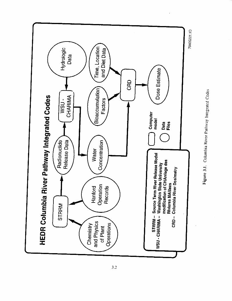
Measured and Modeled Dose Estimates. The first steps in estimating doses involve deter- mining the radionuclide concentrations of the Hanford reactor effluents that were discharged into the river. These concentrations can then be analyzed to determine radionuclide concentrations in various sections of the Columbia River downstream from Hanford. These data are available in the form of hstorical measurements or through computer simulation. Once the radionuclide concentrations in the river at selected locations are known, the effects of environmental accumulation in aquatic biota and use of the river by humans can be estimated. Doses can then be estimated using food consumption and lifestyle information for representative individuals. Figure 3.1 outlines the computer modeling process for the Columbia River pathway.
Because it was not possible to estimate dose for the Columbia River pathway based entirely upon historical measurements, the TSP determined that modeling was the preferred method for estimating dose.(a) Thus, all steps in the dose estimation process, from source term determination to dose assessment, involve the use of computer models. These models are required for two reasons: 1) measurements of radionuclide concentrations in important environmental media (i.e., water, resident fish, salmon, and shellfish) do not exist for dl necessary locations and time periods (Napier and Brothers 1992; Walters et al. 1992; Denham et al. 1993) and 2) environmental monitoring during later years yielded radioactivity measurements below the detection limit of the measuring instrumentation. Napier and Brothers (1992) investigated the level of detail in modeling and recommended the use of historical measurements supplemented by modeling.
The TSP further recommended(a) that most dose estimating effort be expended for the years from 1956-1965 (the period during which radionuclide releases to the Columbia River are known to have been highest) and that the effort expended to estimate doses for the periods prior to 1955 and after 1965 be appropriate to the releases.
Dominant RadionuclidedPathways. Selection of radionuclides and pathways for detailed examination were first addressed by Napier (199 Ib), who ranked the doses from 7 1 radionuclides identified in detailed measurements made in 1956, 1964, and 1968, plus those estimated to be released during fuel failures. The pathways addressed were drinking water, recreation on or near contaminated water (swimming, boating, or shoreline activities), and consumption of fish. Also addressed were pathways h m imgation with contaminated river water, including consumption of imgated
(a) Memorandum (HEDR Project Document No. 1 1920015), “Recommendations for Further River Pathway Work, FyO?.” from P.C. Ungeman (TSP) to TSP Members and D.B. Shipler (BNW), September 28. 1992.
3.1
I I I
8
3
Y
m 0 3
u"
3.2

produce and animal products, exposure to soils contaminated by the water, and inhalation of resuspended dusts from such soils. Of the radionuclides originally investigated, five were identified as important for their potential radiation dose (phosphorus-32, copper-64, zinc-65, arsenic-76, and neptunium-239) with four more considered to be of marginal importance (sodium-24, scandium-46, chromium-5 1, and manganese-56) (Napier 199 lb, p. vii). The imgation-related pathways were shown to be of secondary importance.
In addition, Freshley and Thome (1992) evaluated the contribution of radionuclides to the Columbia River via groundwater from the Hanford Site. This investigation dealt with potential doses via the river pathways as defined in Napier (1991b), as well as the potential doses from riparian wells (Freshley and Thome 1992, pp. 8.1-8.6) and offsite wells (Freshley and Thorne 1992, pp. 6.81-6.84). The general conclusion of this report was that these sources contributed minimal amounts to individual dose.
The model design specification in the HEDR feasibility study (Napier 1991a) considered the results of the previous two studies, and included in the feasibility study calculations eight radionuclides (all those suggested in Napier [ 1991bJ except scandium-46, which was omitted because of lack of data and marginal significance to dose) and all of the direct river pathways of drinking, recreation, and fish consumption. The doses resulting from this modeling were presented in the Columbia River Pathway Reporr (PNL 1991, p. 2.13).
The TSP adopted "dose decision levels," the lower threshold values below which research efforts to define dose should be minimized.(a) These were incorporated into the HEDR Modeling Approach (Shipler and Napier 1992, p. 17) for the Columbia River pathway, by stating, "If, upon consideration. it is determined that any given pathway has the potential to add more than 5% to the total dose for any individual at a time when the dose exceeds the TSP guidelines, it will be ... added to the main models.. . . "
Walters et al. (1992, Section IO) re-investigated all major river-related exposure pathways. The pathway of consumption of resident fish was again found to dominate the results. Consumption of anadromous fish was noted to be a lesser contributor. The imgation-related pathways were again shown to result in small doses. Napier and Brothem (1992) combined the results of the Walters et ai. (1992) dose analysis, the TSP dose decision levels, and a value-of-information analysis to provide a set of recommendations to the TSP for further work. Napier and Brothers (1992, pp. 6.1-6.6) recom- mended that the pathways related to irrigation, shoreline exposure, and inhalation be dropped, because they contributed only small amounts to the total dose. They recommended including resident fish, anadromous fish, waterfowl, oysters, drinking, and swimmingboating pathways in the final c alcu 1 ati om.
A set of interim source terms was made available by efforts of TSP member, M. A. Robkin, in early 1993. Napier (1993) addressed the pathways recommended in Napier and Brothers (1992) using the TSP source term data As a result of this computation, the final selection of five radionuclides
(a) Unpublished report (HEDR Project Document No. 12910094), "Scoping Document for Determination of Temporal and Geographic Domains for the HEDR Project" by B. Shleien (TSP), adopted by the TSP at meeting on February 20-22. 1992, p. 9.
3.3

(sodium-24, phosphorus-32, zinc-65, arsenic-76, and neptunium-239) was made.(a) The Napier and Brothers (1992) scoping study also provided supporting data for the selection of the locations for which doses are reported. In addition, Napier (1993, Appendix B) summarized the doses presented in all Hanford Site annual environmental monitoring reports from 1956 through 1972. These summaries helped define the time period for which calculations are made.
9 Thus, the five key radionuclides used as input to the dose calculations were sodium-24, phosphorus-32, zinc-65, arsenic-76, and neptunium-239. Although it did not contribute significantly to dose, chromium-51 was used for validating the modeling of the river transport of radionuclides because it was virtually always present in detectable concentrations. For the sake of completeness and to satisfr public inreresr, the source terms for manganese-56, gallium-72, yttrium-90, iodine- 13 1, and gross beta were also estimated even though these radionuclides did not contribute significantly to dose.
Section 3.1 explains the "source term" model used for determining the radionuclide concentra- tions at their point of origin; Le., as they entered the Columbia River at Hanford. The section also includes an explanation of the physical mechanisms by which the radionuclides entered the river and which radionuclides were chosen for input to other models that estimate transport down river, concen- trations in foods affected by the Columbia River, and finally the doses experienced by persons exposed through various pathways. The following subsections explain the methods used in the transport, concentration, and dose assessment models (Sections 3.2, 3.3, and 3.4, respectively).
3.1 Source Term Model
The possible consequence of radionuclide releases to individuals has been addressed by starting with estimates of the amount and timing of those releases (Le., the source term). Determining the source term is necessary when concentrations of radionuclides in environmental media are too low to be measured or when monitoring was not comprehensive enough to address all radionuclides, loca- tions, and exposure pathways. Source term release estimates were derived from the large amount of information that exists in government- and contractor-generated documents, plus articles in various technical journals concerning radioactive releases to the Columbia River from Hanford reactor opera- tions. The HEDR Project has produced radionuclide estimates on a monthly basis for 11 radio- nuclides, plus gross beta activity, over the entire period of single-pass reactor operation, 1944-1971 (Heeb and Bates 1994).
Source term estimation covers the radionuclides released during the operation of the eight Hanford Site single-pass production reactors: B, C, D, DR, F, H, KE, and KW. N Reactor, which recirculated the primary cooling water within its core and did not discharge directly to the river, was not included in the scope of Heeb and Bates (1994). N Reactor releases are, however, included in the Hanford annual report doses presented in this report.
(a) Letter (HEDR Project Document No. 07930232), "Key Radionuclides for River Pathway," from J. E. Till (TSP) to D. B. Shipler (BNW), April 12, 1993.
3.4

The information used to reconstmt radionuclide releases to the Columbia River comes from measurements of radionuclide concentrations in reactor effluent before the effluent was discharged to the river. The reconstruction also depends on a quantitative reconstruction of reactor operations to determine the mount of radioactive materials produced by the reactors. This reconstruction has been accomplished and documented by Heeb and Bates (1994). The information was obtained from moni- toring records of Hanford effluent. Although such data were plentiful, the number of radionuclides that were monitored and the time periods covered were limited. The data in the historical documents are generally reported on a monthly basis. Although some information does exist on daily reactor operations, the information does not cover the entire 1944-1971 time period. Therefore, Heeb and Bates (1994) present source term information by the month. This approach has been deemed adequate for estimating annual doses. Where gaps in information occur, reasonable estimates of the missing historical measurements were supplied by using statistical analysis of available effluent measurements together with Monte Carlo uncertainty modeling.
3.1.1 Mechanism for Source Term Releases to River
10 Radioactive materials generated at the Hanford Site were produced primarily by fission of uran- ium in the reactors, activation of nonradioactive materials, and by fission and activation of naturally occumng uranium-238 by neutron capture in reactor coolant water during reactor operations.
Water from the Columbia River was pumped into a water treatment plant where chemicals were added to adjust the pH, decrease turbidity, and lnhibit corrosion of the supply piping and reactor process tubes. The processed river water was then filtered, held in clear wells, and pumped into large holding tanks. From the tanks, it was pumped to the reactor inlet to be used as reactor cooling water.
11 The cooling water passed from the inlet piping into the gap between the fuel-element surface and the process tube. During its brief passage through the reactor core region (1 to 2 seconds), water at the lnlet river temperature (0 to 20°C) was heated to over 100°C in the highest-powered tubes. The cooling water was also subjected to a neutron flux of between 1013 and 1014 neutrons per square centimeter per second. This neutron flux caused trace impurities in the cooling water to be converted into radioactive species. This process is called neutron activation and accounts for the bulk of the radioactive emissions to the Columbia River. The hot effluent water (bulk temperature as high as 95OC) was discharged from the reactor into external retention basins located near the Columbia River. After cooling thermally and allowing time for the shortest-lived radionuclides to decay, the basin water was discharged to the Columbia River. The capacities of the retention basins were designed to allow a nominal holdup time of 2.4 to 4.0 hours. With design modifications to increase reactor power in 1957, however, the reactor bulk flows in the B, D, DR, F, and H reactors were increased to almost three times the original designed flows. This resulted in holdup times nearer to 1 hour, which decreased the time allowed for radioactive decay.
As reactor operation continued, films of oxides and entrained materials built up on both process tubes and fuel elements. Beginning in 1945, slumes of abrasive diatomaceous earth were injected into the inlet cooling water during full power operation. This material mechanically removed some of the film from fuel elements and process tubes. These purges continued until final shutdown in 1971. Because the film being removed contained radionuclides, purges resulted in temporarily increased radioactive discharges to the Columbia River. However, radionuclide releases to the river during
3.5

radioactive discharges to the Columbia River. However, radionuclide releases to the river during diatomaceous earth purges have been determined to be minor compared to releases from routine operations, fuel-element failures, and activation of corrosion products in the process tubes (Heeb and Bates 1994).
11.13 Hanford experienced nearly 2000 fuel-element failures in the eight single-pass reactors. A fuel- element failure occurred when the aluminum cladding was breached, allowing coolant water direct access to the inadiated uranium. The result was a release of fission products and activation products to the effluent water. Every attempt was made to remove the fuel element with the failure as soon as possible. The reactor was shut down as soon as a fuel-element failure was indicated. For purposes of the HEDR Project, information on the reactor, date, and classification of each failure was extracted from Hanford reports. This information was used to estimate the release contributions of iodine-13 1 and neptunium-239 from fuel-element failures. These two radionuclides (the first a fission product and the other a decay product of uranium-239, which is a neutron capture product of uranium-238) were widely used as indicators of fuel-element failures. Heeb and Bates (1994, pp. 4.27 and 4.29) estimated that 44.9 percent of the iodine-131 and 11.9 percent of the neptunium-239 releases came from fuel- element failures. Most of the iodine-I31 and neptunium-239 resulted from n a W uranium in the Columbia River water.
3.1.2 Radionuclide Release Estimates
Figure 3.2 shows the annual releases of the five key radionucIides used for dose calculations. These totals (in curies/year) are the median values of 100 stochastic realizations (Heeb and Bates 1994). Monte Carlo stochastic modeling was used to estimate uncertainties in the source term release estimates. The estimates of radionuclide releases to the Columbia River include the calculated radionuclide decay from the time of release from the reactors to the time of actual discharge to the river. A complete description of the source term uncertainty is presented in Heeb and Bates (1994).
11 ' Figure 3.3 shows the activity of the five key radionuclides that existed throughout the Columbia River and adjacent area in the Pacific Ocean. The amount that existed at any time was estimated by accounting for the radionuclide production in the Hanford reactors and the decay in the environment. Because of the very short (15-hour) half-life of sodium-24, no more than 3500 curies of sodium-24 ever existed at any time, even though nearly 1,400,OOO curies were released during 1960 alone. Conversely, almost 80,OOO curies of zinc-65, the most long-lived of the five radionuclides, existed (mainly in the Pacific Ocean) during the highest year of 1962, although no more than 56,000 curies of this radionuclide were ever released in one year. The effect of radioactive decay is demonstrated by Figures 3.2 and 3.3. The amount of radionuclides released does not necessarily comlate to radiation dose.
3.2 River Transport Model
A computer model of the flow and transport of Columbia River water was used to provide monthly average concentrations of radionuclides at specific locations'along the river. The model, documented by Walters et al. (1994), estimates the radioactivity in the Columbia River after the river received cooling water effluent from the eight Hanford single-pass reactors. The reconstruction of
3.6

1,400,000
1,200,000
1,000,000
800,000
600,000
400,000
200,000
0
Date
Figure 3.2. Key Radionuclides Released to the Columbia River by Year, 1944-1971
d m w d d d z z z
I- d m ?
Q) d m F
Date
Figure 3 3 . Rivedocem Radionuclide Burden, 1944-1971
3.7

historical water concentrations is limited to the area downriver from the reactors where the cooling water was returned to the river. Specifically, the concentrations of radionuclides are estimated from Priest Rapids Dam downstream to just below Portland, Oregon. Within that len,oth of river, the TSP selected 12 locations where radionuclide concentrations were to he reconstructed, beginning with January 1950 and extending through January 1971.(a) Figure 3.4 shows the domain of the Columbia River pathway computer model, including the Columbia River, the Hanford Site, and the locations used for reconstruction of radionuclide concentrations.
3.2.1 Development of the Columbia River Transport Conceptual Model
An extensive Columbia River literature review was conducted and reported in Walters et al. (1992) . That report provides a brief description of reactor operations, effluent water composition, and routine and accidental radionuclide releases. The report also discusses special studies conducted by Hanford contractors of reactor effluent plume dispersion, shoreline radiation surveys, and downriver travel times as well as routine monitoring results and preliminary dose calculations.
Based on an evaluation of data and information found in Hanford and offsite literature, the TSP recommended(b) that surface-water concentrations be determined for use in dose estimates. Walters et al. (1992) recommend that a one-dimensional hydraulic model be used to estimate the route of effluent from the reactors to downstream locations where dose is to be estimated. The TSP further recommended that reactor source term data be used with the hydraulic routing model to reconstruct radionuclide concentrations because of insufficient Columbia River historical measurements. Measurements downstream from Pasco, Washington, were very limited or nonexistent, and before 1958 only gross beta measurements were available at any location on the river.
Further recommendations by the TSP were that the effects on water concentrations of the reactor effluent plume and the sediment uptake and release of radionuclides should be based upon the results from past field studies and historical measurements and not directly calculated by the model. A com- plex effluent plume analysis was not needed because the horizontal mixing width can be adequately determined using a simple hand calculation and vertical mixing occurs rapidly near the reactor outfalls. For sediment uptake effects, a simple empirical approach using correction factors developed from experiments with the selected model estimates and historical measurements. The effects of the plume were to he limited to the Hanford Reach, while the sediment uptake effects may have extended the length of the Columbia River.
Hydraulic computer modeling required the use of a one-dimensional, unsteady flow model capable of routing water and radionuclide releases downstream from the Hanford reactors for the required time span and locations. The code selected for the Columbia River transport work was CHARIMA (CHAmage des RIvieres MAillees) which simulates sediment transport in looped river systems (Holly et al. 1993). CHARIMA was selected because it fulfills the following modeling requirements specified by the TSP (Farris 1993):
(a)
(b)
Letter (HEDR Project Document No. 07930224). "HEDR Project Locations for Calculation of Radionuclide Concentrations in the Columbia River (14)," from D. E. Walker, Jr. (TSP) to W. A. Bishop (TSP), April 2, 1993. Memorandum (HEDR Project Document No. 11920015). "Recommendations for Further River Pathway Work. FY93." from P.C. Ungernan (TSP) to TSP Members and D.B. Shipler (BNW), September 28, 1992.
3.8

TI 0 L a n.
0 0 v) E 0
Q 0 0 A
5 c
- L
0
3.9

use monthly or weekly source term data use monthly, weekly, or daily river flow data establish the point of complete effluent plume mixing below the reactors assume complete mixing below McNary Dam make simple radionuclide decay corrections for travel time in river water downstream make simple assumptions about waterhediment interactions use one-dimensional analysis (longitudinal only) use unsteady flow and reservoir routing use a simple empirical approach for sediment uptake/release.
Moreover, CHARIMA can accommodate tributary inflows, multiple channels within a river, and the presence of dams and reservoirs. It also has the capability to route contaminants to any specified location.
CHARIMA is a f~te-difference code that simulates unsteady flow (flood wave) hydraulics and nonuniform sediment transport in open channel (unimpounded) systems such as rivers and canals. The code can simulate the operation of dams and reservoirs and input a constituent (such as a contaminant or heat) in the routing scheme. For the Columbia River computations, the CHARIMA code was mod- ified to allow for radionuclide decay. The modified code is called WSU-CHARIMA to differentiate i t from the acquired version. The sediment transport capabilities of the CHARIMA code were not used because the required amount of historical data for the Columbia River were not available.
3.2.2 Model Validation
The Columbia River model was validated by a process that compared historical measurements with those estimated by the model. The validation of the water concentrations computed by WSU- CHARIMA was accomplished in two distinct phases. First, the Columbia River hydraulics were validated by comparing the model-estimated water levels with the measured river stage. The second and final stage of validation was the estimation of water concentrations at river locations where his- torical measurements were available. Validation was accomplished by computer-modeled routing of the reactor source term estimates for chromium-51 from the reactor locations downstream to the historical river monitoring locations and comparing the computed with the historically monitored results.
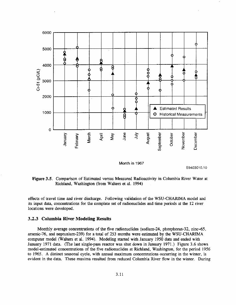
A sample comparison of the estimated water concentrations with historical measurements is shown in Figure 3.5. In general, the two data sets agree well. With the exception of the September 1967 data, all estimated monthly average concentrations shown in Figure 3.5 fall within the range of the monthly measurements. This sample is typical of the comparisons between the estimated and measured water concentrations. For some locations and radionuclides, the comparisons are not as close. The agreement between estimated and measured data is further discussed in Walter; et al. (1994).
Sediment correction factors were found to be unnecessary (Walters et al. 1994). The validation exercise showed that while some sediment interaction did occur, there was no consistent correlation with season or river discharge. The impact of sediment effects was much less important than the
3.10
6000
5000
4000
2 oa G
3000 9
2000
1000
0
Month in 1967 S9403010.10
Figure 3.5. Comparison of Estimated versus Measured Radioactivity in Columbia River Water at Richland, Washington (from Walters et al. 1994)
effects of travel time and river discharge. Following validation of the WSU-CHARIMA model and its input data, concentrations for the complete set of radionuclides and time periods at the 12 river locations were developed.
3.2.3 Columbia River Modeling Results
Monthly average concentrations of the five radionuclides (sodium-24, phosphorus-32, zinc-65, arsenic-76, and neptunium-239) for a total of 253 months were estimated by the WSU-CHARIMA computer model (Walters et al. 1994). Modeling started with January 1950 data and ended with January 1971 data. (The last single-pass reactor was shut down in January 1971.) Figure 3.6 shows model-estimated concentrations of the five radionuclides at Richland, Washington, for the period 1956 to 1965. A distinct seasonal cycle, with annual maximum concentrations occurring in the winter, is evident in the data. These maxima resulted from reduced Columbia River flow in the winter. During
3.11

late spring and summer, the melting snow in the Cascades and Rocky Mountains increased the river flow, causing increased dilution of Hanford originated radionuclides. During parts of July and August 1966, all Hanford reactors were shut down because of a labor strike. The reduced radionuclide releases during these two months are included in the source term, river transport, and dose modeling.
3.3 Radionuclide Concentrations in Aquatic Organisms
In order to estimate doses to individuals who ingested aquatic organisms (fish, waterfowl, Willapa Bay oysters, and salmon) taken from or near the Columbia River, the radionuclide concentra- tions in those organisms must be determined. Several different approaches were used to estimate the concentrations of radionuclides in aquatic organisms. Each approach relied heavily on historical measurements collected by Hanford researchers, other state and federal government agencies, and nongovernment agencies, such as universities. The approaches used to estimate the radionuclide concentrations in fish and waterfowl, Willapa Bay oysters, and salmon are explained below.
3.3.1 Fish and Waterfowl Bioconcentration Factors
The concentration of radioactive material in fish and waterfowl can be related to the radionuclide concentration in the water in which that organism lives and feeds (NCRP 1984). This relationship is a simplistic correlation that accounts for ecosystem interactions between the water and the organism. This simplistic approach was used to develop bioconcentration factors (BCFs) that directly relate the radionuclide concentration in the organism to that in the Columbia River water. A large database of measured radionuclide concentrations in Columbia River fish, waterfowl, and water was assembled and used by HEDR Project staff to develop BCFs.
Historical data from the Columbia River have been used to estimate BCFs specific to the river. As noted in summaries of BCFs in Vanderploeg et al. (1975) and Poston and Klopfer (1988), fish BCFs vary greatly depending on site-specific conditions of a river system. For a given aquatic system, BCFs are generally independent of location and year but dependent upon radionuclide, animal species, and the season of the year.
The development of BCFs for fish resident in the Columbia River is discussed at length in Thiede et al. (1994). That report includes a detailed description of the data used and the resulting BCFs that were used in the dose calculations. All BCFs are for the edible flesh and not the whole fish. BCFs were determined using the following model:
BCF = F / W (3.1 )
where BCF = bioconcentration factor (literkilogram) F = concentration of the radionuclide in fish or waterfowl muscle (picocuriehulogram)
W = concentration of the radionuclide in water (picocurie/liter).
7.13

When historical sample data are lacking, the radionuclide concentration in fish and waterfowl can be approximated using estimated BCFs for the Columbia River and the water concentrations modeled by WSU-CHARIMA (Walters et al. 1994), as follows:
F = B C F * W , (3.2)
where F =
BCF = w, =
radionuclide concentration in fish or waterfowl at a given location (picocurie/kilogram) bioconcentration factor (liter/kilogram) WSU-CHARIMA estimated water Concentration of a radionuclide (radionuclide and location specified by F) (picocurie/liter).
3.3.1.1 Fish Bioconcentration Factors
Table 3.1 presents the median BCFs for the five key radionuclides in this study (sodium-24, phosphorus-32, zinc-65, arsenic-76, and neptunium-239). Thiede et al. (1994) present a ful l description of the statistical uncertainty associated with these BCFs. Table 3.1 presents the BCFs for five radionuclides for three types of Columbia River fish (omnivorous and first- and second-order predators) and with cool and warm seasons. Omnivorous fish include bullhead, catfish, suckers, whitefish, chiselmouth, chub. sturgeon, minnows, and shiners. First-order predators include perch, crappie, punkinseed, and bluegill. Second-order predators include bass, trout, and squawfish. (Salmon and steelhead are treated separately and are discussed in Section 3.3.3.) The cool season for the Columbia River is considered December through May, and the warm season June through November.
3-3-12 Waterfowl Bioconcentration Factors
Historical data listing radionuclides in waterfowl were documented as early as 1946 (Parker and Norwood 1946a; 1946b). Hanf et al. (1992) describe the historical documents for waterfowl samples for 1945-1972. These documents show that before 1958, only gross beta was measured. By 1960, individual radionuclides could be measured. In general, zinc-65 and phosphorus-32 were the only radionuclides routinely measured in waterfowl taken from the Columbia River and adjacent areas. These historical measurements provide a basis from which to calculate the Columbia River BCFs for waterfowl (Thiede et al. 1994).
17 Two general types of ducks were included in this study: diver ducks (which eat small fish and invertebrates) and puddle ducks (which eat near-surface water plants and ,omin crops). Diver ducks found on the Columbia River include goldeneye, bufflehead, canvasback, merganser, coot, scaup, and ruddyduck. Puddle ducks include mallards, gadwall, pintail, shovelers, widgeon, and wood duck. Geese feed in a manner similar to puddle ducks and were included in this summary because historical data were available. Approximately 72 percent of the 1684 measurements were for puddle ducks, 17 percent for diver ducks, and 11 percent for geese. The waterfowl BCFs used in the dose calcula- tions are listed in Table 3.2. Bioconcentntion factors were not calculated for sodium-24, arsenic-76, and neptunium-239 because these radionuclides were typically not detected in waterfowl samples. These BCFs are for all seasons. because no seasonal dependence was found in the historical sampling data. Thiede et al. (1994) present a full description of the uncertainty associated with these BCFs.
3.14

Table 3.1. Median Bioconcentration Factors for Columbia River Fish Using Historical Fish Measurements and WSU-CHARIMA Estimated Water Concentrations (from Thiede et al. 1994)
Radionuclide
sodium-24
sodium-24
phosph01~s-32
phosphor~s-32
phosph01~s-32
phosphor~s-32
zinc-65
zinc-65
zinc-65
zinc-65
zinc-65
zinc-65
arsenic-76
neptunium-239
Fish Type/Season
omnivorous
all predators
omnivorous cool season
omnivorous warm season
all predators cool season
all predators warm season
omnivorous cool season
omnivorous warm season
1st-order predators cool season
1st-order predators warm season
2nd-order predators cool season
2nd-order predators warm season
all species and seasons
all species and seasons
Median Bioconcentration
Factor
80
2.1
420
1500
76
980
130
220
97
250
67
110
240
21
3.15

Table 3.2. Median Bioconcentration Factors for Columbia River Waterfowl (from Thiede et al. 1994)
Median Bioconcentration Radionuclide Factor &fig)
phosph01~s-32 290
zinc-65 44
Figure 3.7 shows zinc-65 concentrations in aquatic organisms. Concentrations of all five key radionuclides were calculated using the estimated water concentration data shown in Figure 3.6 and the BCFs described above.
3.3.2 Willapa Bay Shellfish Data
Zinc-65 and phosphorus-32 concentrations in aquatic organisms near the mouth of the Columbia River were monitored as early as 1959. Walters et al. (1992) give a summary of average radionuclide concentrations at Willapa Bay for 1959-1977. Oysters from Willapa Bay were found to contain mea- surable amounts of Hanford originated radionuclides @sag et al. 1973). Hanf et al. (1992) describe documents containing historical information on radionuclides in shellfish (primarily bivalve mollusks). Information from these references was compiled into a database. Thiede et al. (1994) list summary data from this database for phosphorus-32 and zinc-65 for locations such as Willapa Bay, Astoria, Cannon Beach, Coos Bay, Seaside Beach, Tillamook Bay, and Agate Beach. Oysters generally contained hgher concentrations of zinc-65 than did other marine organisms (Foster and Wilson 1962).
The total reactor output of zinc-65 by year (Heeb and Bates 1994) was compared, using a linear regression coefficient, to the average zinc-65 concentration in oysters at Willapa Bay. The coefficient was 0.0019 picocurie/grm per curie/year (R2 = 0.83, calculated without an intercept term), indicating that for each curie of zinc-65 released during a given year, there would be 0.0019 picocurie/gram of zinc-65 in oysters. Using this information, it is possible to approximate the activity of zinc-65 in oysters for years for which there is little or no historical data (1944-1959). Then, the following equa- tion was used to convert reactor production to radioactivity in oysters for any given year:
WBO = 0.0019 c (1.3)
where WBO = activity of zinc-65 in Willapa Bay oysters (picocurie/gram) 0.00 19 = estimated regression coefficient (picocurie/gram per curie/year)
C = number of curies of zinc-65 released from Hanford production reactors during a given year (curie) (from Heeb and Bates 1994).
3.16
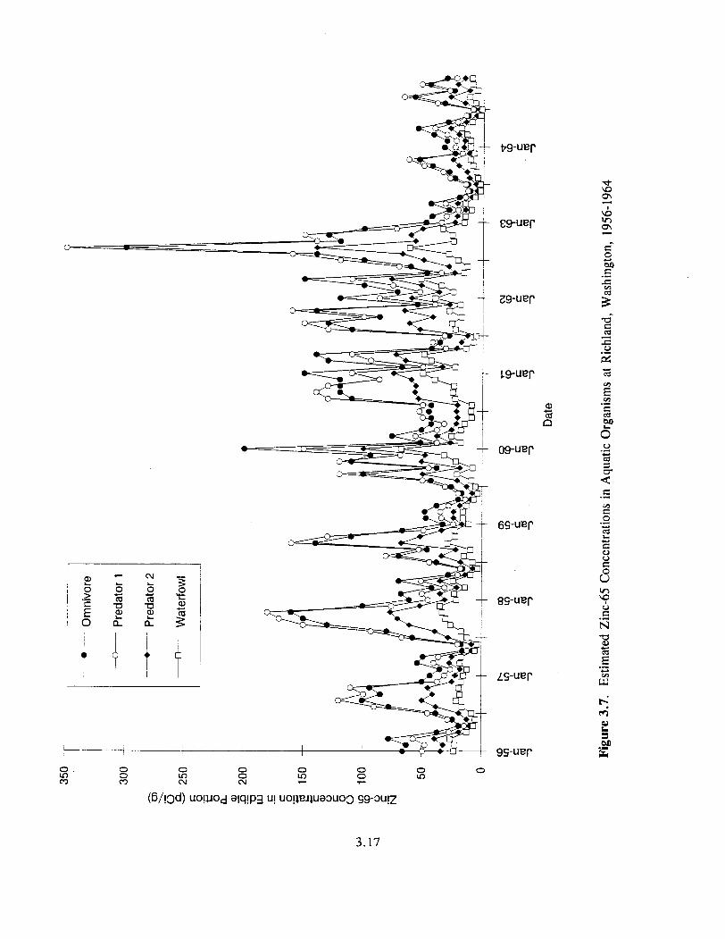
L c. f L
W r. 3 M kl .I
3.17

3.3.3 Salmon Data
Anadromous species (fish that live part of their lives in freshwater and part in salt water), such as chinook salmon, sockeye salmon, coho salmon, and steelhead trout, travel up the Columbia River to spawn. Walters et al. (1992, Figure 4.5) summarize the time periods when these species are found in the Columbia River. According to Foerster (1968), sockeye, in common with other Pacific salmon species, do not feed once they enter fresh water and head upstream to their natal spawning area. Evidence for this lack of feeding comes from stomach content analysis, decreased fat and protein content, and atrophy of digestive organs. Feeding usually ceases prior to spawning (Brown 1957; Foerster 1968; Meehan 1991), and the fish rely on reserves of fat and protein stored up during their ocean residence to reach their natal spawning area
Juvenile salmon and steelhead feed during their 3- to 24-month river migration downstream to the ocean (Oregon Department of Fish & Wildlife and Washington Department of Fisheries 1993). However, for the purpose of dose assessment, it is assumed that anadromous species such as salmon and steelhead in the Columbia River took in radionuclides primarily while feeding on organisms in the ocean. These ocean organisms may have accumulated radionuclides from both Columbia River discharge and atmospheric nuclear weapon’s test deposition. Accumulation of radionuclides in upstream anadromous species may have depended on the radionuclide accumulation from food sources and accumulation from radionuclide concentrations in the Columbia River. The radionuclide concen- tration in the fish muscle would then depend on what the fish had accumulated before it moved into the river and on the concentration of radionuclides in the Columbia River water. Data for 47 historical samples of salmon caught in the Columbia River show that 37 samples were at or below the minimum detection limit (0.1 picocurie/gram) for zinc-65. The rest of the samples varied from just above the detection limit to a maximum of 13 picocuries/gram. The median value for zinc-65 was 0.6 picocurie/gram.
The TSP determined that doses from salmon and steelhead should be calculated using two approaches.(a) The first approach would be to use available historical measurements. Using this approach, a default value of 1 picocurie/gram was used for the concentration of zinc-65 in salmon and steelhead flesh for all years (corresponding with the median monitored concentration of 0.6 picocurie/ gram, which was rounded to 1 picocurie/gram). The second approach assumed that the salmon spend their entire lives in the Columbia River and accumulate radionuelides as do resident species.
The second approach (treating salmon and steelhead as resident species in the Columbia River) was selected by the TSP because it provided an upper limit for doses from ingestion of salmon and steelhead. This approach was used to estimate the uncertainty in salmon and steelhead doses. The BCF values for resident second-order predators (trout, bass, and squawfish) were used to model all radionuclide concen- trations in salmon. If actively eating, salmon would have feeding habits similar to those of second-order predators (Le., they would feed on smaller fish). This approach yielded zinc-65 concentrations in salmon ranging from about 1 picocurie/gram to 100 picocuries/gram. Figure 3.8 shows the 47 hstorical measurement points (many points overlap), the default concentration of 1 picocurie/gram specified by the first approach, and the concentrations based on the BCFs of resident second-order predators (as specified
(a) Direction given by the Technical Steering Panel (TSP) at the October 7-9, 1993 meeting held in Richland, Washington.
3.18

5 2
a m 5 .- 3
m P P
LL u
U Q e,
.- z I-' v) w
C 0 .- +I
e, C Q 0 C 0 0
3 m Q
F
e, - v-
n
F
0
3.19

by the second approach). The second approach gives salmon concentrations that are 10 to 100 times larger than the actual monitoring results. Therefore, the second approach should be considered an overestimation of the actual concentrations and doses calculated with this approach are likely to overestimate the actual doses.
3.4 Dose Assessment
Once the source terms and concentrations were estimated, standard dose assessment methods were used to translate the radionuclide concentrations in key environmental media into the radiation dose that could have been received by an individual. The environmental media of concern for the Columbia River pathway include treated and untreated drinking water, resident fish, waterfowl, salmon, and shellfish. Also evaluated were external exposures from swimming, boating, and shoreline activities.
The following subsections introduce the use of the computer code designed to estimate doses to individuals via these environmental media, explain the calculation of doses, and define the categories of individuals assessed for doses from the Columbia River pathway.
3.4.1 Capabilities of the Columbia River Dosimetry Code
The requirements for the computer code used to estimate radiation doses resulting from the Columbia River pathway are documented in FruTis (1993) and specify that the code estimate the radiation from a number of pathways and radionuclides. The computer code that was developed. Columbia River Dosimetry (CRD), uses water concentrations of sodium-24, phosphorus-32, zinc-65, arsenic-76, and neptunium-239 calculated by the WSU-CHARIMA model (see Section 3.2).
Radionuclide-dependent water treatment factors are used to account for the moderate reduction in radionuclides in drinking water after treatment in a municipal treatment system. An untreated drinking water pathway is also included where no such reduction is assumed.
CRD supports the deterministic estimation of environmental accumulation and dose. This means that the code calculates a single-point estimate of all media concentrations and doses. (A stochastic analysis was performed to investigate the uncertainty and sensitivity of input parameters and calculated doses in the CRD code. The methodology for and results of that analysis are presented in Section 5.0.)
CRD calculates doses for 12 specific river segments (refer to Figure 3.4). The segment names and approximate locations are as follows:
1. Ringold (from below reactor areas to north of Richland) 2. Richland (from north of Richland to above the Yakima River) 3. KennewicldPasco (from below the Yakima River to the Snake River) 4. SnakeWalla Walla rivers (from below the Snake River to near McNary Dam) 5 . Umatilla/Boardman (from near McNary Dam to near Arlington, Oregon) 6. Arlington (Arlington, Oregon vicinity)
3.20

7. John Day Dam/Biggs (from below Arlington, Oregon, to near Biggs, Oregon) 8. Deschutes River (Deschutes River mouth vicinity) 9. The Dalles/Celilo (The Dalles/Celilo vicinity) 10. Klickitat River (Klickitat River mouth vicinity) 11. White SalmodCascade Locks (from White Salmon River to Bonneville Dam) 12. Lower River (from below Bonneville Dam to Columbia River mouth)
On the recommendation of the TSP,(a) doses from ingestion of two environmental media with location-dependent concentrations but not directly river-dependent concentrations were also estimated, bringing the number of locations of interest for dose assessment to 14. The two additional doses were those resulting from ingestion of shellfish from Willapa Bay and from salmon and steelhead caught at any location in the Columbia River.
In addition, for each category of individual for whom a radiation dose was estimated, specific parameters relating to exposure are supplied in CRD. Each of the following exposure parameters can be specified by month in the CRD code:
il- b.
d. e. f.
h.
J.
C.
U a'
1.
river use - swimming (hours/month) river use - boating (includes fishing and shoreline activities) (hours/month) untreated drinking water ingestion (liters/month) treated drinking water ingestion (liters/month) resident fish (omnivore) ingestion (kilograms/month) resident fish (first-order predator) ingestion (kilograms/month) resident fish (second-order predator) ingestion (kilogamshnonth) waterfowl ingestion (kilograms/month) Willapa Bay shellfish ingestion (kilognms/month) Columbia River anadromous fish (salmordsteelhead) ingestion (kilograms/month).
3.4.2 Equations in the Columbia River Dosimetry Code
The basic equations implemented in the CRD code are shown below. ' Shown first are equations for radionuclide concentrations in Columbia River water. Then, there are the equations for doses from environmental media. See Snyder et al. (1994) for details about the selection of the parameter values. Doses were calculated using methods described in ICRP (1977). Doses were estimated for each radionuclide, location, and month. As recommended by the TSP,(b) the results include estimations of effective dose equivalent @DE) as well as estimations of dose equivalent to the red bone marrow (RBM) and to the lower large intestine (LLI). These two critical organs were selected because they are the organs that would have received the highest radiation doses.
(a)
(b)
Letter (HEDR Project DocumenTNo. 07930224). "HEDR Project Locations for Calculation of Radionuclide Concentrations in the Columbia River (14)," from D.E. Walker, Jr. (TSP) to W.A:Bishop (TSP), April 2, 1993. Letter (HEDR Project Document No. 08910177), "Scoping Documents for Determination of Temporal and Geographical Domains for the HEDR Project" from B. Shleien (TSP) to Distribution, July 26, 1991.
3.2 1

3.42.1 CRD Code Equations for Radionuclide Concentrations
The radionuclide concentration in untreated Columbia River water for each location and month is calculated as follows:
c, = c, P (3.4)
where C, = concentration of radionuclide in Columbia River water at point of human contact (picocuriefliter)
C, = cross-section average concentration of radionuclide in Columbia River water (picocurie/liter)
P = plume correction factor for each location (unitless).
The plume correction factor accounts for the difference in the shoreline concentration relative to the average concentntion across the river. At Ringold, the radionuclide concentrations are greater on the Hanford shore than on the Ringold shore (Walters et al. 1994). The WSU-CHARIMA code calcu- lates the average concentration in the Columbia River at each downstream location. The plume cor- rection factor allows the determination of the actual shoreline concentration using the WSU- CHARMA calculated values. The plume correction factors used are 0.5, 1.1, and 0.9 for the Ringold, Richland, and Pasco locations, respectively. The derivation of these factors is based on in-stream studies on the Columbia River and are explained in more detail in Walters et al. (1994). At all other lOCatiOnS, the river is assumed to be fully mixed and no plume correction is warranted. The plume correction factor for Ringold is for the east shore, which is accessible to the general population. The Richland and Pasco locations are for the shoreline locations with the maximum estimated concentrations.
The radionuclide concentration in the edible flesh of resident fish and waterfowl €or each location and month is calculated in CRD as:
c, = c, BCF (3.5)
where C, = concentration of radionuclide in fish or waterfowl (picocurie/lulogram) C, = cross-section average concentration of radionuclide in Columbia River water
(picocurie/liter) BCF = bioconcentration factor for a given species of fish or waterfowl (picocuriekilogram
per picocuriefliter).
The bioconcentration factors are those defined in Section 3.3.1 above.
3.4.2.2 CRD Code Equations for Doses
Ingestion of Water. The monthly dose to each organ from ingestion of treated and untreated water for each location and month is calculated as:
3.22

Dw = C,,, [(e -* f,>+ %I DFi (3.6)
where Dw =
c, =
% I = Rw, -
f, = Rw2 -
h =
-
- DF, =
effective dose equivalent or organ dose equivalent from ingestion of all drinking water (mil li rem/month) concentration of radionuclide in Columbia River water a point of human contact (picocuries/liter) radionuclide-specific radiological decay constant (per day) holdup time for treated drinking water (days) amount of treated drinking water ingested (liters/month) water treatment transmission factor (unitless) amount of untreated drinking water ingested (liters/month) dose conversion factor for ingestion (millirem/picocurie).
The ingestion dose conversion factors are from DOE (1988). The drinking water transmission factors have been derived from historical measurements at water treatment facilities in Richland, Kennewick, and Pasco, Washington. The transmission factors account for the radioactivity that passes through the treatment process and is not removed. The transmission factors for the five key radionuclides of interest are listed in Table 3.3. Supporting information for these values is presented in detail in Snyder et al. (1994):
Table 33. Transmission Factors for Five Key Radionuclides
Radionuclide Transmission Factor sodium-24 0.9 phosph01~s-32 0.38 zinc-65 0.39 arsenic-76 0.5 neptunium-239 0.67
Ingestion of Resident Fish and Waterfowl. The monthly dose to each organ from resident fish and waterfowl ingestion for each location and month is calculated in CRD as:
(3.7)
where D, = effective dose equivalent or organ dose equivalent from ingestion of resident fish or waterfowl (millirem/month)
C, = concentration of radionuclide in fish or waterfowl (picocuries/kilognm) Rf = amount of fish or waterfowl ingested (kilograms/month) h = radiological decay constant (per day)
thf = holdup time for resident fish or waterfowl (days) DF, = dose conversion factor for ingestion (millirem/picocurie).
3.23
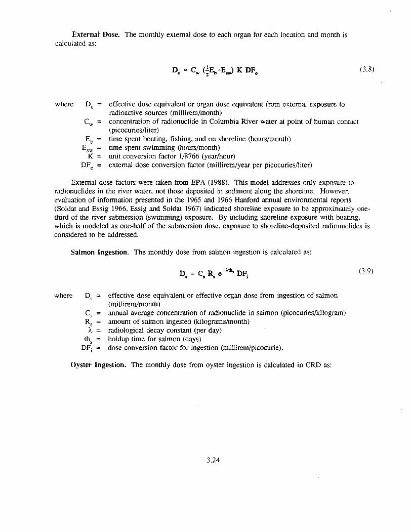
External Dose. The monthly external dose to each organ for each location and month is calculated as:
De = C, (:%+E,) K DF, (3.8)
where De = effective dose equivalent or organ dose equivalent from external exposure to radioactive sources (millirem/month)
C, = concentration of radionuclide in Columbia River water at point of human contact (picowriesfliter)
E,, = time spent boating, fishing, and on shoreline (hours/month) E,, = time spent swimming (hours/month)
K = unit conversion factor 1/8766 (yearhour) DFe = external dose conversion factor (millirem/year per picocuriesfliter)
External dose factors were taken from EPA (1988). This model addresses only exposure to radionuclides in the river water, not those deposited in sediment along the shoreline. However, evaluation of information presented in the 1965 and 1966 Hanford annual environmental reports (Soldat and Essig 1966, Essig and Soldat 1967) indicated shoreline exposure to be approximately one- third of the river submersion (swimming) exposure. By including shoreline exposure with boating, which is modeled as one-half of the submersion dose, exposure to shoreline-deposited radionuclides is considered to be addressed.
Salmon Ingestion. The monthly dose from salmon ingestion is calculated as:
D, = c, R, DF,
where D, = effective dose equivalent or effective organ dose from ingestion of salmon (millirem/month)
C, = annual average concentration of radionuclide in salmon (picocuriesllulogram) R, = amount of salmon ingested (kilograms/month) h = radiological decay constant (per day) th, = holdup time for salmon (days)
DF, = dose conversion factor for ingestion (millirem/picocurie).
(3.9)
Oyster Ingestion. The monthly dose from oyster ingestion is calculated in CRD as:
3.24

-Ath, Do = C, R, e DFi (3.10)
where Do = effective dose equivalent or effective organ dose from ingestion of oysters (millirem/month)
C, = annual average concentration of radionuclide in oysters (picocurieshulogram) R, = amount of oysters ingested (kilograms/month) h = radiological decay constant (per day)
tho = holdup time for oysters (days) DF, = dose conversion factor for ingestion (millirem/picocurie).
3.4.3 Representative Individual Definitions
To estimate the dose to individuals who were exposed to the Columbia River in the past, a set of representative (theoretical) individuals has been selected. The characteristics of these individuals are intended to approximate those of selected segments of the general population. The characteristics of the representative individuals do not match any known person. The representative individuals are used to estimate the doses to these selected population segments.
.I Maximum representative individual - Assumed to have been a significant user of the Columbia River. l h s individual had maximum or near maximum ingestion rates for resident fish and waterfowl and spent time in or on the river.
.I Typical representative individual - Typical of the average individual residing near the Columbia River. No resident fish were ingested by this type of individual. This corresponds to information provided in Soldat (1968), Beetle (1972), and Endres et al. (1972). Doses for individuals of this second type who did ingest fish can be inferred from the doses calculated for the maximum representative individual.
.I Occupational representative individual - A worker who is assumed to have been exposed at work. This individual could have been a feny or barge worker or someone who spent a significant amount of time on the river and who ingested no fish or shellfish.
Tables 3.4 through 3.6 list characteristics of the representative individuals.
Reference values were defined for each representative individual’s usage and intake rates for each pathway. The usage and intake values vary by month. Holdup times (ie., the times between removal from the river and ingestion) must also be defined for the reference individuals because of the short half-lives of some of the radionuclides evaluated. The assumed holdup times are shown in Table 3.7. Assumptions are based on values used in historic estimates of intake rates in the region as reported in Hanford Site annual environmental reports from 1958 to 1970, which are summarized in Soldat et al. (1986), and on the authors’ judgment.
3.25
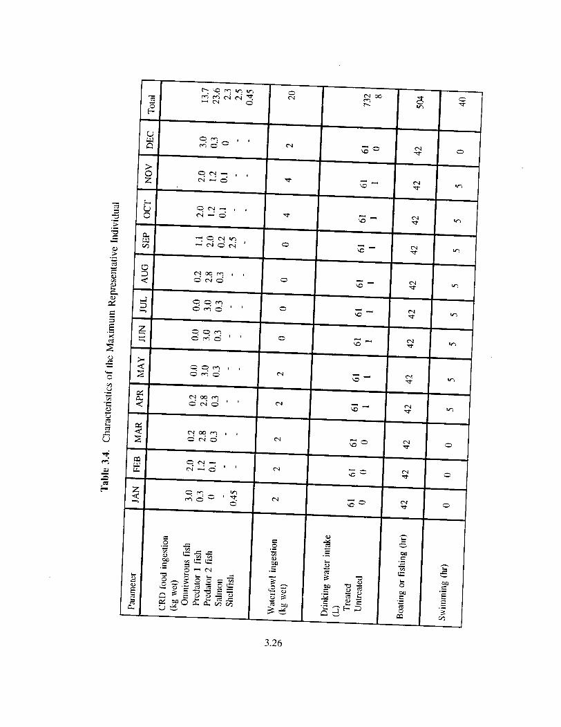
LL q
3.26

l m N
- 0
0 - 0
0
w.
Z ' I C 0
I Z ' 0 0
r - I m vi
, " ' ICI m
m m
m r- m ' m
vr
0
, " ' 0
, " '
Z ' O I
h L
5
E E 3
M E .-
.- v!
3.27

3.28
L ' G
' G
' G
0 d N
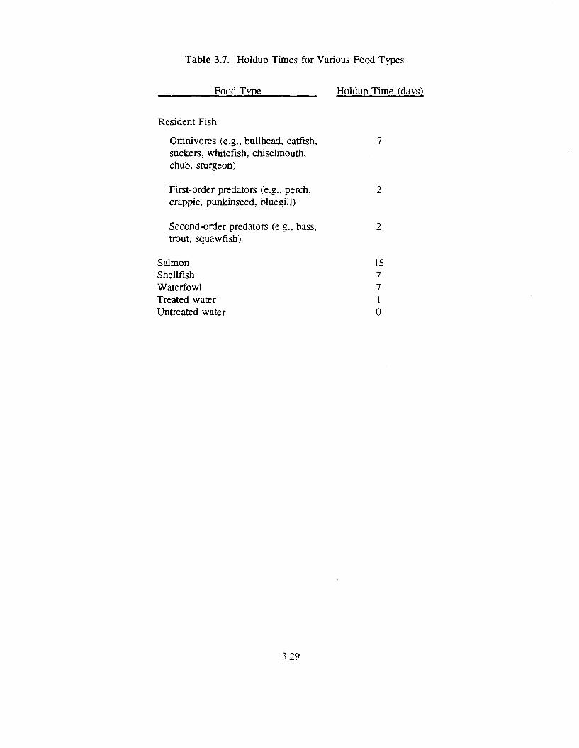
Table 3.7. Holdup Times for Various Food Types
Food Type
Resident Fish
Omnivores (e.g., bullhead, catfish, suckers, whitefish, chiselmouth, chub, sturgeon)
First-order predators (e& perch, crappie, punkinseed, bl uegi 1 I )
Second-order predators (e.g., bass, trout, squawfish)
Salmon Shellfish Waterfowl Treated water Untreated water
Holdup Time (days)
7
2
2
15 7 7 1 0
3.29

4.0 Results
Estimates of doses to individuals from reactor releases to the Columbia River for the years 1944- 1992 are presented in this section All dose estimates are prepared using deterministic tech- niques, which use a single estimate for each input parameter for a model and return a single output estimate result. Such techniques have no built-in allowance for uncertainty. (See Section 5.0 for information on uncertainty in the dose estimates and the sensitivity of the estimated doses to specific input parameter values.)
Results of the estimations of annual doses from 1944-1992 are presented in Section 4.1. Results are given for three dose estimation approaches for three consecutive time periods: screening dose calculations for 1944-1949, detailed dose calculations for January 1950 through January 1971, and dose calculations using data from Hanford annual environmental reports for 1971-1992. These three methods are based on the level of detail required for doses for the three time periods. These dose results are summarized for effective dose equivalent to a maximum representative individual and results are compared to the earlier feasibility study doses found in the Columbia River Pathway Report (PNL 1991).
Section 4.2 provides results for the exposure pathways, comparing the parameters contributing the most to doses received by three types of representative individuals at Richland, Washington, and downstream of the Bonneville Dam. Section 4.3 presents the doses estimated for ingestion of salmon and steelhead, and Section 4.4 presents the doses for ingestion of Willapa Bay oysters.
4.1 Annual Doses, 1944-1992
The dose estimation method used for 1944 through 1992 depended on the time considered. Screening calculations were performed for 1944 through 1949, detailed dose calculations were performed for 1950 through January 1971, and Hanford annual reports were consulted for February 1971 through 1992. The screening calculations were performed for a single location (Ringold, Washmgton), the detailed dose calculations were performed for 12 locations, and the doses obtained from annual reports were for single locations between Ringold and Pasco, Washington.
The level of detail in the dose calculations was based on the magnitude of radionuclide releases for the time period, Based on earlier HEDR Columbia h v e r source term and dose calculations (PNL 1991; Napier and Brothers 1992; Walters et al. 1992), the TSP recommended that dose calculations for 1950-1970 be the most detailed.(a) The modeling techniques discussed in Section 3.0 were devel- oped in response to this recommendation. The time period for detailed calculations was expanded to include January 1971 in order to incorporate the last monlli of single-pass reactor operations. Less rigorous dose assessment techniques were used for the other time periods because radionuclide releases were much lower during those years.
(a) Memo (HEDR Project Document No. 11920015), "Distribution of Recommendations for FY 93 River Work," from P. C. Klingeman (ET Subcommittee Chair) to M. Power and K. CharLee (Washington State Department of Ecology), September 28, 1992.
4.1
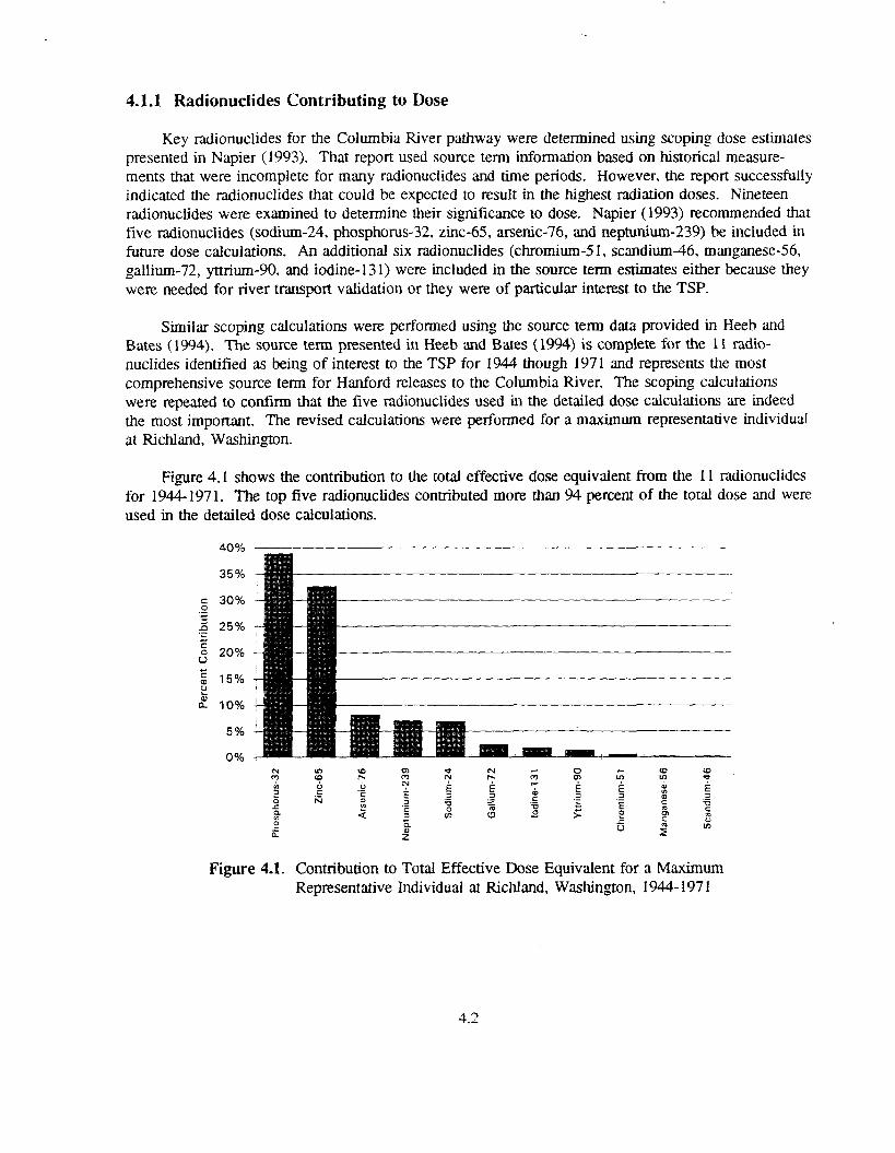
4.1.1 Radionuclides Contributing to Dose
Key radionuclides for the Columbia River pathway were determined using scoping dose estimates presented in Napier (1993). That report used source term information based on historical measure- ments that were incomplete for many radionuclides and time periods. However, the report successfully indicated the radionuclides that could be expected to result in the highest radiation doses. Nineteen radionuclides were examined to determine their significance to dose. Napier (1993) recommended that five radionuclides (sodium-24, phosphorus-32, zinc-65, arsenic-76, and neptunium-239) be included in future dose calculations. An additional six radionuclides {chromium-5 1, scandium46, manganese-56, gallium-72, yttrium-90, and iodine- 13 1) were included in the source term estimates either because they were needed for river transport validation or they were of particular interest to the TSP.
Similar scoping calculations were performed using the source term data provided in Heeb and Bates ( 1994). The source term presented in Heeb and Bates (1994) is complete for the 1 1 ndio- nuclides identified as being of interest to the TSP for 1944 though 1971 and represents the most comprehensive source term for Hanford releases to the Columbia River. The scoping calculations were repeated to confirm that the five radionuclides used in the detailed dose calculations are indeed the most important. The revised calculations were performed for a maximum representative individual 3t Richland, Washington.
Figure 4.1 shows the contribution to the total effective dose equivalent from the 11 radionuclides for 1944-1971. The top five radionuclides contributed more than 94 percent of the total dose and were used in the detailed dose calculations.
c 30%
2 25%
0
._ - L c
6 20%
5%
0%
Figure 4.1. Contribution to Total Effective Dose Equivalent for a Maximum Representative Individual at Richland, Washington, 1944- 197 1
4.2

4.1.2 Screening Dose Calculations, 1944- 1949
Screening doses to a maximum representative individual at Ringold, Washington, were calculated for this report using median values for each radionuclide provided in Heeb and Bates (1994). The WSU-CHARIMA model was not used for these simple calculations. The calculations used a simplified river transport model that assumed an average Columbia River flow rate of 120,000 cubic feet per second and 14-hour travel time from the reactors to Ringold. Assumptions used in these calculations regarding dosimetry and exposure parameters were described in Sections 3.4.2 and 3.4.3.
Table 4.1 presents the doses to a maximum representative individual at Ringold, Washington. Doses to the maximum representative individuals at all locations were dominated by the ingestion of fish containing zinc-65 and phosphorus-32. Table 4.1 shows that the effective dose equivalent ranged from 2 millirem/year in 1944 to 26 millirem/year in 1949.
Table 4.1. Doses to a Maximum Representative Individual at Ringold, Washmgton, 1944-1949, from Ingestion'of Fish
Effective Dose Key Pathway1 - Year Eauivalent (mrem/vr) Radionuclides
1944 2 fishfa-65, P-32
1945 23 fishfa-65, P-32
1946 18 fishfa-65, P-32
1947 16 fishfa-65, P-32
1948 18 fish/&-65, P-32
1949 26 fish/Zn-65, P-32
4.1.3 Detailed Dose Calculations, January 1950-January 1971
The doses estimated for this period are the most detailed because they represent the years when an individual using the river would have received the highest dose. particularly the years 1956-1965. The doses were estimated on a monthly basis using detailed estimates of source term, river transport, and human exposure. The dose estimates were computed for each month to maximize the detail included in the dose calculations and to account for any seasonal effects. Radionuclide concentrations in the river, bioconcentration factors, and human characteristics for ingestion and exposure are all highly dependent on the month of the year.
The CRD model (Farris 1993; Baker and Farris 1994) was used to perform these dose calculations using the monthly source term and river transport estimates documented above (Heeb and Bates 1994; Walters et al. 1994). Doses for this period were calculated for 3 types of representative individuals, 12 specific river locations, 5 radionuclides, and 253 months (January 1950 through
4.3

January 1971) and include ingestion of Willapa Bay shellfish and Columbia River salmon. Doses were calculated for two specific organs, red bone marrow and lower large intestine, in addition to the effective dose equivalent (whole body dose).
The appendix lists monthly estimates and annual totals of the effective dose equivalent and effective doses to red bone m m w and lower lage intestine. These dose estimates are provided for the three representative individual types at 12 locations. Figures 4.2, 4.3, and 4.4 show estimated doses for the three representative individual types at selected locations. Doses ax each successive downriver location below Pasco decrease as radioactive decay and river dilution decrease the local radionuclide concentrations. The estimated doses are greatest for the maximum representative individual and lowest for the typical representative individual.
Prior to October 1963, the municipal water supply for the City of Richland, Washington, was drawn from Yakima River water. The Richland municipal water supply after September 1963 was taken from the Columbia River. Figure 4.3 shows the impact of the water source on the doses to the typical representative individual at Richland. Before 1963, the doses to a typical individual at Richland were less than those at Pasco and other locations. After 1963, the doses were highest at Richland. The doses for the maximum and occupational representative individuals do not show the effect because those doses were dominated by exposure pathways other than dnnYcing water; Le., consumption of fish or external exposure.
Within the 1950-1971 time period, the doses for all representative individual types are lowest during the periods 1950-1955 and 1965-1971. The doses peak during the late 1950s and early 1960s the period of greatest radionuclide releases to the Columbia River (see Section 3.1 and Figure 3.2). The decrease in annual dose in 1959 was a result of slightly lower radionuclide releases and increased river flow during that year. These two factors combined to produce dose estimates that were 30 to 40 percent lower for 1959 than for either 1958 or 1960.
The doses shown in Figures 4.2, 4.3, and 4.4 are the total doses summed over a number of pathways and radionuclides and given as effective dose equivalent. Detailed information on the contributing pathways and radionuclides is presented in Section 4.2. For all monthly dose estimates, it was assumed that salmon contained 1 picocurie/gram of zinc-65. An alternate approach for estimating doses from salmon and steelhead is presented in Section 4.3.
4.1.4 Doses from Hanford Annual Reports, 1971-1992
Annual reports summarizing environmental monitoring and offsite radiation impacts have been prepared by Hanford contractors every year since 1957 (Soldat et al. 1986). These reports are pre- pared one to two years after the subject year and are available to the public. Each report contains an estimate of the radiation dose to a maximum representative individual for the subject year. Because dose estimation methods are constantly evolving, different assumptions regarding dosimetry, exposure parameters, and modeling were used to amve at the doses reported for February 1971 through 1992. However, the doses as presented do provide an overview of the overall magnitude and trend of the doses.
4.4
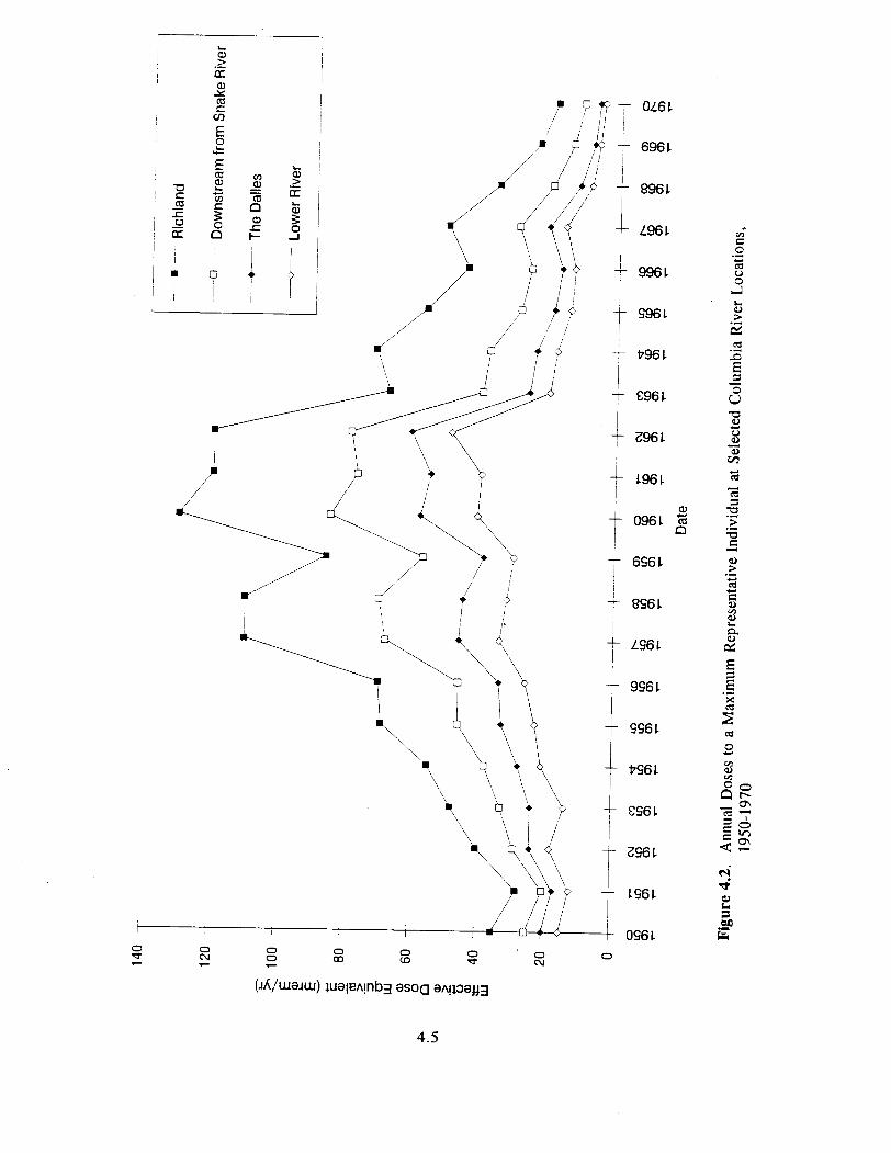
a r I- + L96L
I i T 9961
I S96L
+ P961
I a + 0961 E I
-f 6S61
- 8S6L 1 I
LS6L
4 9S6L
I
SS6 L
PS6L
1 IS61 ' Z96L t lS6L
4.5
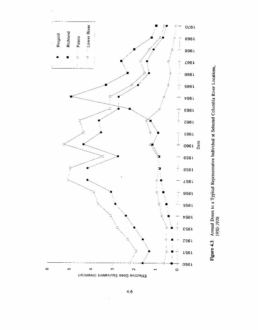
/ OL6 1 F. 0-
Y m
4.6

I L. a > U a Y m c a
0
.- I
E L u-
- 6961
896 1 / s /" /
8
I 996 1
4.7

Doses for 1971 through 1992 are presented in Table 4.2. The most recent year for which a Hanford annual environmental monitoring report is available is 1992. The r e p n for 1993 will be available in late 1994. Dose estimates after 1973 are significantly lower than estimates made for the peak dose years of 1955-1965. Doses dropped significantly after the shutdown of the last single-pass production reactor in January 1971. N Reactor releases during the mid-1980s resulted in doses of a few millirem per year and are included in the doses presented in Table 4.2.
4.1.5 Complete Dose History
Dose results from the three dose estimation approaches (screening calculations, detailed dose calculations, and doses obtained from annual reports) are combined and shown in Figure 4.5. These doses are summarized in Table 4.3. Over 93 percent of the total dose occurred during the 1950-1971 time period. Figure 4.5 shows doses received by a maximum representative individual at Ringold, Washington, from 1944-1992. Doses for the maximum individual at other locations would be lower than the doses at Ringold, Washington. The annual doses for a typical representative individual are approximately 10 to 40 times lower than those received by a maximum representative individual. Doses for the typical representative individual at Pasco were higher than at Ringold or Richland. Doses for an occupational representative individual were estimated to be lower than those received by a maximum representative individual at all locations.
Doses presented in this report are for three types of representative adults. Doses to children have not been specifically calculated for the three types of representative individuals for all locations and months. Agedependent doses for children can be inferred from the doses to the typical represen- tative individual adult. For typical representative individuals, both children and adults, the exposure is dominated by consumption of drinking water. The radiation dose from a given intake of any of the five key radionuclides in this study is as much as seven times greater for a child than for an adult (Phipps et al. 1991). However, children consume as little as one-sixth the amount of drinking water and water-based foods as adults (EPA 1989). The net result is that doses for children for any specific year could be a factor of 1.5 to 2 higher than the adult doses for the typical representative individual.
The exposure assumptions for the other two types of representative individuals are not applicable to children. Doses to the occupational representative individual are applicable to an adult who is working on or near the river for 2900 hours/year. The maximum representative individual is estimated to consume large amounts of fish and waterfowl and cannot be considered representative of a child’s exposure. Dietary studies done in the late 1960s indicate that most children did not consume game birds or fish from the Columbia River (Soldat and Honstead 1968; Endres et al. 1972). Body burden measurements of 5099 children during 1965-1969 indicated that the average whole body dose to a child in the Richland, Pasco, Kennewick area was approximately I milliredyear.
4.1.6 Comparison to Feasibility Study Dose Estimates
The scope of the feasibility study (PNL 1991) included dose calculations for 1964-1966 and locations from the areas of the reactors to McNary Dam. Figure 4.6 shows a comparison of median doses presented in the feasibility study Columbia River Pathway Report (PNL 1991) with doses estimated for this report. Doses are shown for maximum and typical representative individuals
4.8

Table 4.2. Hanford Annual Report Doses, 1971-1992
Year
1971
1972
1973
1974
1975
1976
1977
1978
1979
1980
1981
1982
1983
1984
1985
- 1986
1987
1988
1989
1990
1991
1992
- Maximum Individual Total
Body or Effective Dose Equivalent (mrem)
3(a)
$4
2
0.03
0.012
0.04
0.2
0.03
<0.09
<O.l(a)
O.l@)
0.4@)
0.01
0.057
0.07
0.05
0.03
0.02
0.039
0.0 16
0.009
0.02
Reference
Soldat, Price, and McCormack. 1986. PNL-5795
Bramson and Carley. 1973. BNWL-1727.
Soldat, Price, and McCormack. 1986. PNL-5795
Fix. 1975. BNWL-1910
Spear, Fix, and Blumer. 1976. BNWL-1979
Fix, Blumer, Hoenes, and Bramson. 1977. BNWL-2142
Houston and Blumer. 1978. PNL-2614
Houston and Blumer. 1979. PNL-2932
Houston and Blumer. 1980. PNL-3283
Sula and Blumer. 1981. PNL-3728
Sula, McCormack, Dirks, Price, and Eddy. 1982. PNL-4211
Sula, Carlile, Price, and McCormack. 1983. PNL-4657
Soldat. 1989. PNL-7135
Soldat. 1989. PNL-7135
Sold& 1989. PNL-7135
Pacific Northwest Laboratory. 1987. PNL-6120
Jaquish and Mitchell. 1988. PNL-6464
Jaquish and Bryce. 1989. PNL-6825
Jaquish and Bryce. 1990. PNL-7346
Woodruff and Hanf. 1991. PNL-7930
Woodruff and Hanf. 1992. PNL-8148
Woodruff and Hanf. 1993. PNL-8682
(a) Annual report presents doses for air and river pathways combined, and it is not possible to separate doses by pathway. Doses presented here are the sum of air and river pathways and are an overestimate of the Columbia River dose. Annual report presents doses from consumption of foods containing radioactivity released via the air and river pathways combined. It is not possible to separate doses by source.
(b)
4.9
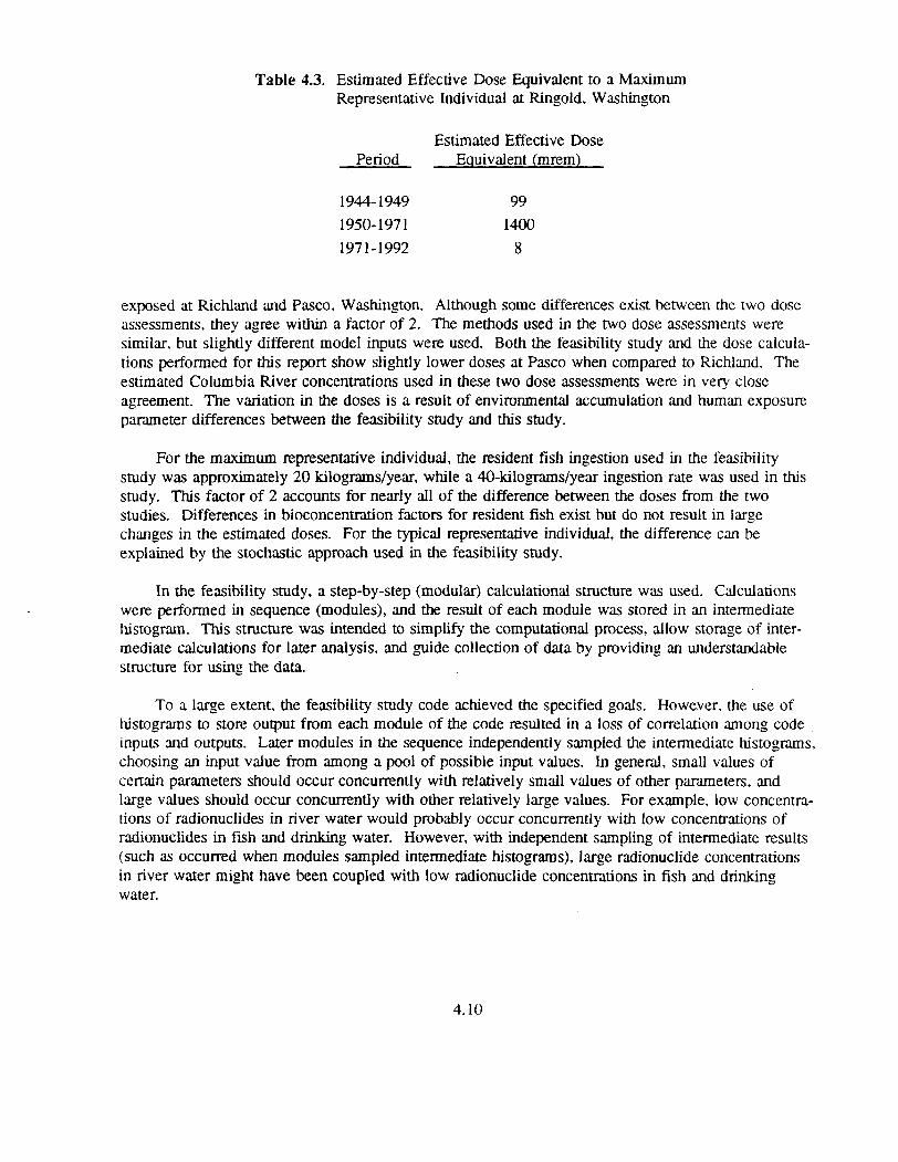
Table 4.3. Estimated Effective Dose Equivalent to a Maximum Representative Individual at Ringold, Washington
Estimated Effective Dose Period Equivalent (mrem)
1 944- 1949 99 1950- 197 1 1400 197 1-1992 8
exposed at Richland and Pasco, Washington. Although some differences exist between the two dose assessments, they agree within a factor of 2. The methods used in the two dose assessments were similar, but slightly different model inputs were used. Both the feasibility study and the dose calcula- tions performed for this report show slightly lower doses at Pasco when compared to Richland. The estimated Columbia River concentrations used in these two dose assessments were in very close agreement. The variation in the doses is a result of environmental accumulation and human exposure pameter differences between the feasibility study and this study.
For the maximum representative individual, the resident fish ingestion used in the feasibility study was approximately 20 kilograms/year, while a 40-kilognms/year ingestion rate was used in h s study. This factor of 2 accounts for nearly all of the difference between the doses from the two studies. Differences in bioconcentration factors for resident fish exist but do not result in large changes in the estimated doses. For the typical representative individual, the difference can be explained by the stochastic approach used in the feasibility study.
In the feasibility study, a step-by-step (modular) calculational structure was used. Calculations were performed in sequence (modules), and the result of each module was stored in an intermediate histogram. This structure was intended to simplify the computational process, allow storage of inter- mediate calculations for later analysis, and guide collection of data by providing an understandable structure for using the dam.
To a large extent, the feasibility study code achieved the specified goals. Howe.ver, the use of histograms to store output from each module of the code resulted in a loss of correlation among code inputs and outputs. Later modules in the sequence independently sampled the intermediate histograms, choosing an input value from among a pool of possible input values. In general, small values of certain parameters should occur concurrently with relatively small values of other parmeters, and large values should occur concurrently with other relatively large values. For example, low concentra- tions of radionuclides in river water would probably occur concurrently with low concentrations of radionuclides in fish and drinking water. However, with independent sampling of intermediate results (such as occurred when modules sampled intermediate histograms), large radionuclide concentrations in river water might have been coupled with low radionuclide concentrations in fish and drinking water.
4.10

Y) W c,
.- F c, v) w Y z a 0. W
- c3 S C c 6
L Z661 1 1661
L 6861 L 8861
L86 1 986 1 486 1 P86 1 E86 1 I 286 1
'i 0661
1 E; 1 6L61 - 8L61 I LL61
9L61 4L61
i PL61 1- EL61
696 1 896 1 L96 1
In N
0 0
E96 1 Z96 1 196 1 096 L 646 1 896 1 L46 1 946 1 446 1
4P6 A-
Ll PP6
0 In
In N
0
W m C
n
4.11
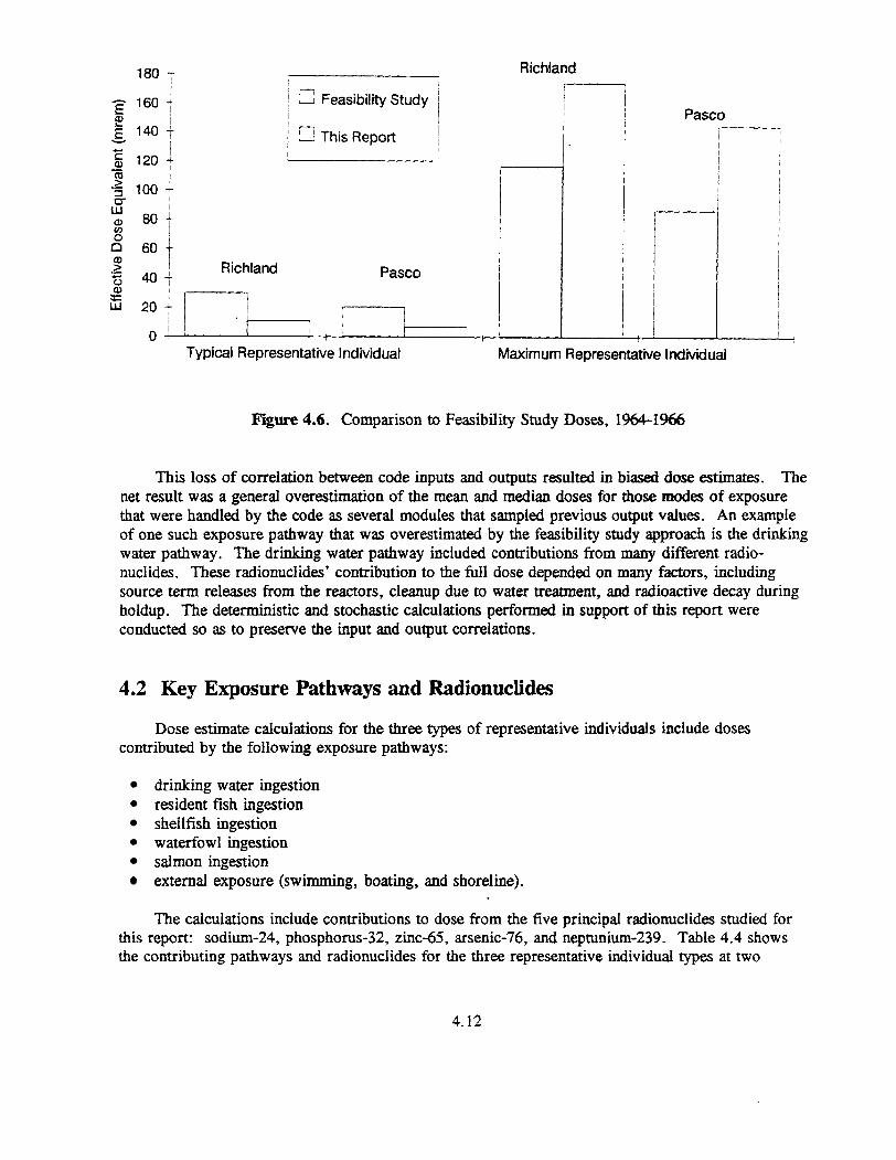
Richland
I ! f
I
180 -j-
1 1
' a Feasibility Study I ' 2 This Report , I I I
Pasco
1 I
Typical Representative Individual Maximum Representative Individual
Figure 4.6. Comparison to Feasibility Study Doses, 1964-1966
This loss of correlation between code inputs and outputs resulted in biased dose estimates.
-
The net result was a general overestimation of the-mean and median doses for those modes of exposure that were handled by the code as several modules that sampled previous output values. An example of one such exposure pathway that was overestimated by the feasibility study approach is the drinking water pathway. The drinking water pathway included contributions from many different radio- nuclides. These radionuclides' contribution to the full dose depended on many factors, including source term releases from the reactors, cleanup due to water treatment, and radioactive decay during holdup. The deterministic and stochastic calculations performed in support of this report were conducted so as to preserve the input and output correlations.
4.2 Key Exposure Pathways and Radionuclides
Dose estimate calculations for the three types of representative individuals include doses contributed by the following exposure pathways:
drinking water ingestion resident fish ingestion shellfish ingestion waterfowl ingestion salmon ingestion external exposure (swimming, boating, and shoreline).
The calculations include contributions to dose from the five principal radionuclides studied for this report: sodium-24, phosphorus-32, zinc-65, arsenic-76, and neptunium-239. Table 4.4 shows the contributing pathways and radionuclides for the three representative individual types at two
4.12

b? 0 0 7 0 0 7 - c
7
in
c
5 r2
- -
w C w
4.13
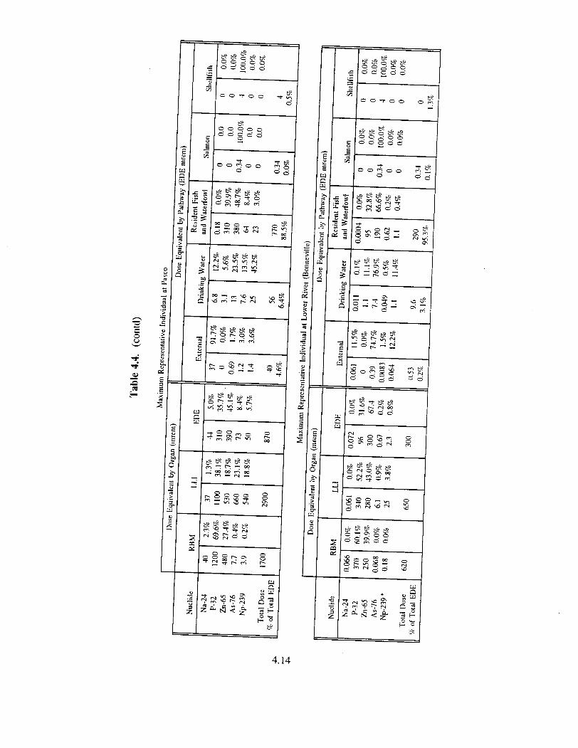
.- - 1 1 w 0 B C
4.14

e o o o c o " 2
c-" 0 0 0 0 0 0 0
0
C-oe**e 9 9 9 9 9 0 0 0 0 0
€3 o o o o o " 8
€3 o o o o o " 8
C-oee*e 0 0 0 0 0 0 0 0 0 0
€3 o o 3 0 0
€3 o o o o o O8
E P z
4.15
locations: Pasco, Washington, and the lower river below Bonneville Dam. The 1956-1965 time period is presented because it is the period of highest dose for all locations and all representative individual types. As discussed in Section 3.3.3, salmon doses were calculated assuming 1 picocurie/ gram of zinc-65 in all salmon.
The pathways contributing to the effective dose equivalent at Pasco, Washington, varied depending on the representative individual types:
0 For the maximum representative individual, the largest contribution to effective dose equivalent came from the ingestion of resident fish containing zinc-65 and phosphorus-32.
For the typical representative individual, the largest contribution to effective dose equivalent came from the ingestion of treated drinking water containing neptunium-239, zinc-65, arsenic-76, and sodium-24, in that order.
For the occupational representative individual, the largest contribution to effective dose equivalent came from external exposure to sodium-24. However, the dose to O C C U ~ ~ ~ ~ O R ~ representative individuals at locations downriver from Richland came from the ingestion of untreated drinking water containing zinc-65.
.
Similar pathways dominated the doses calculated for corresponding representative individuals located downstream from Pasco:
For maximum representative individuals, contributions from fish ingestion dominated the dose.
For both typical and occupational representative individuals, contributions fmm drinking water dominated the dose.
20 The ingestion of shellfish from Willapa Bay accounted for 40 percent of the effective dose to a typical representative individual below the Bonneville Dam. However, the 10-year total effective dose equivalent for such an individual was approximately 10 millirem (1 milliredyear).
Different radionuclides dominated the effective dose equivalent at Pasco and the Columbia River downstream of Bonneville Dam. Doses estimated for Pasco show a higher contribution from sodium-24 and arsenic-76 than those estimated for downriver locations. This was because of the short half-lives of sodium-24 and arsenic-76 (approximately one day or less for each). Radioactive decay resulted in lower concentrations of these two radionuclides in the river downstream of Pasco. Zinc-65 and phosphoms-32 contribute the most to doses at downstream locations.
4.3 Doses from Ingestion of Salmon and Steelhead
The TSP determined that not enough historical measurements exist on radionuclide concentrations in Columbia River salmon and steelhead to unequivocally determine doses resulting from ingestion of these fish over the 1944-1971 time period. Therefore, doses have k e n calculated using the two approaches described in Section 3.3.3. The first approach relies on the actual historical measurements
4.16
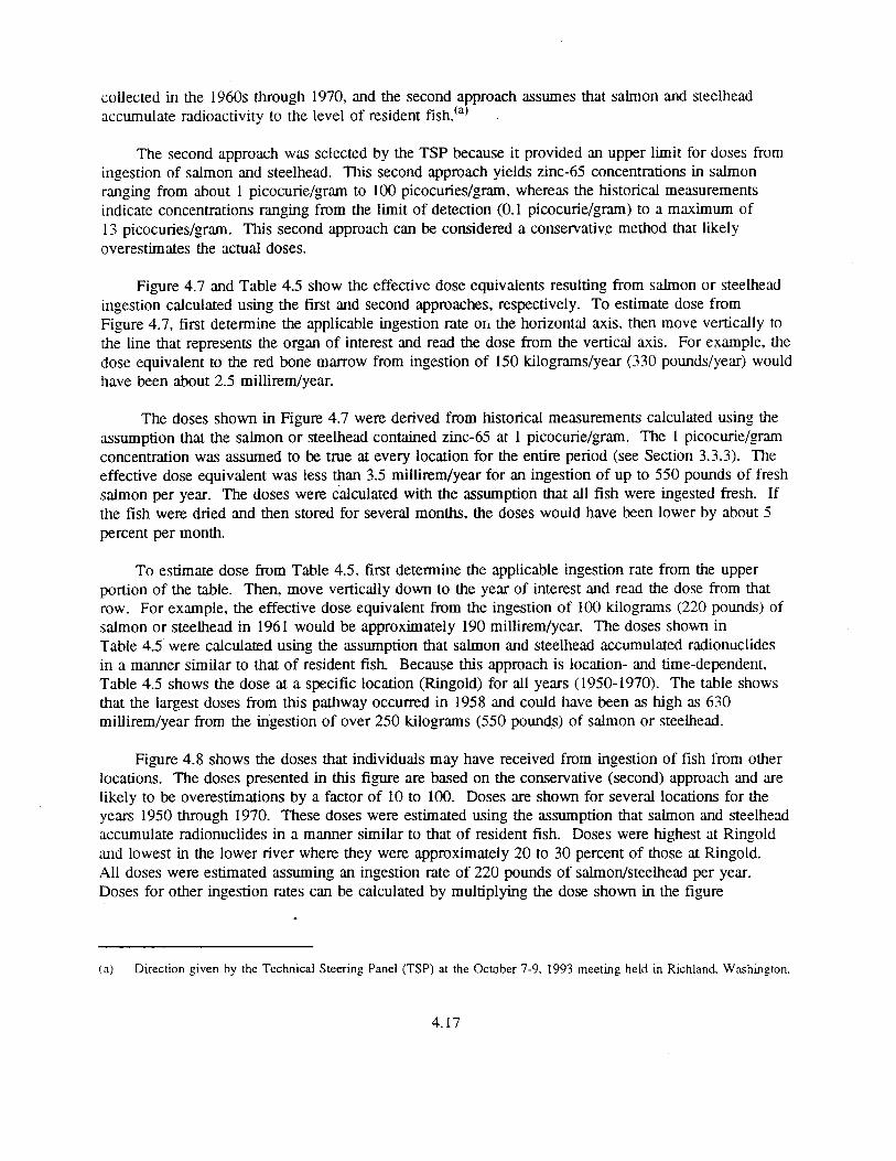
collected in the 1960s through 1970, and the second a proach assumes that salmon and steelhead accumulate radioactivity to the level of resident fish. J
The second approach was selected by the TSP because it provided an upper limit for doses from ingestion of salmon and steelhead. This second approach yields zinc-65 concentrations in salmon ranging from about 1 picocurie/gram to 100 picocuries/gram, whereas the historical measurements indicate concentrations ranging from the limit of detection (0.1 picocurie/gram) to a maximum of 13 picocuries/gram. This second approach can be considered a conservative method that likely overestimates the actual doses.
Figure 4.7 and Table 4.5 show the effective dose equivalents resulting from salmon or steelhead ingestion calculated using the first and second approaches, respectively. To estimate dose from Figure 4.7, first determine the applicable ingestion rate or1 the horizontal axis, then move vertically to the line that represents the organ of interest and read the dose from the vertical axis. For example, the dose equivalent to the red bone marrow from ingestion of 150 kilograms/year (330 pounds/year) would have been about 2.5 millirem/year.
The doses shown in Figure 4.7 were derived from historical measurements calculated using the assumption that the salmon or steelhead contained zinc-65 at 1 picocune/gram. The 1 picocurie/gram concentration was assumed to be true at every location for the entire period (see Section 3.3.3). The effective dose equivalent was less than 3.5 millirem/year for an ingestion of up to 550 pounds of fresh salmon per year. The doses were calculated with the assumption that all fish were ingested fresh. If the fish were dried and then stored for several months, the doses would have been lower by about 5 percent per month.
To estimate dose from Table 4.5, first determine the applicable ingestion rate from the upper portion of the table. Then, move vertically down to the year of interest and read the dose from that row. For example, the effective dose equivalent from the ingestion of 100 kilograms (220 pounds) of salmon or steelhead in 1961 would be approximately 190 millirem/year. The doses shown in Table 4.5 were calculated using the assumption that salmon and steelhead accumulated radionuclides in a manner similar to that of resident fish Because this approach is location- and time-dependent. Table 4.5 shows the dose at a specific location (Ringold) for all years (1950-1970). The table shows that the largest doses from this pathway occurred in 1958 and could have been as high as 630 millirem/year from the ingestion of over 250 kilograms (550 pounds) of salmon or steelhead.
Figure 4.8 shows the doses that individuals may have received from ingestion of fish from other locations. The doses presented in this figure are based on the conservative (second) approach and are likely to be overestimations by a factor of 10 to 100. Doses are shown for several locations for the years 1950 through 1970. These doses were estimated using the assumption that salmon and steelhead accumulate radionuclides in a manner similar to that of resident fish. Doses were highest at Ringold and lowest in the lower river where they were approximately 20 to 30 percent of those at Ringold. All doses were estimated assuming an ingestion rate of 220 pounds of salmonhteelhead per year. Doses for other ingestion rates can be calculated by multiplying the dose shown in the figure
(a ) Direction given by the Technical Steering Panel (TSP) at the October 7-9, 1993 meeting held in Richland, Washington.
4.17

5
- 4.5 k 2 4 z .- 9
Q)
w 3.5 * c 2 3
2.5 w
0 % 2 n
1.5 > 0 1 a
Y= w 0.5
0
meaidwee k
.- c,
W Y r 0 50 1 00 150
0 4 8 13 Fish Consumption
200 250
17 21 s9403010.10z
Figure 4.7. Dose from Consumption of Salmon or Steelhead with 1 Picocurie of Zinc45 per Gram
by the factor of the actual amount ingested divided by 220, as shown in the following example. The dose resulting from ingestion of 100 pounds/year of salmonlsteelhead in 1958 would be
250 mrem/yr * loo lb/p = 114 nnem/yr 220 lb/yx
(4.1)
The doses shown in Figure 4.8 can be considered representative of doses from salmon ingestion in tributaries of the Columbia River using the assumption that salmon and steelhead accumulate radionuclides in a manner similar to that of resident fish. A conservative example is where salmon that migrate to the upper reaches of the Snake River are assumed to have given the same dose as those at the mouth of the Snake River (shown by the second line from the top in Figure 4.8). The doses from ingestion of salmon from other tributaries can be determined using the dose for the location on Figure 4.8 nearest the tributary confluence. Salmon caught above Ringold would not have concentrations of radionuclides higher than at Ringold.
4.18

Table 4.5. Annual Dose from Consumption of Salmon or Steelhead at Ringold(”)
Units kg/yr Wyr
1 b/month meals/wk@)
Year 1950 1951 1952 1953 1954 1955 1956 1957 1958 1959 1960 1961 1962 1963 1964 1965 1966 1967 1968 1969 1970
-
Consumption Rate 10 so 100 1 so 200 250 22 110 220 330 440 550 2 9 18 28 37 46 1 4 8 13 17 21
Effective Dose Equivalent (mem/vr) 7 6 10 10 11 17 13 23 25 15 23 19 23 14 12 14 11 11 7 5 5
35 32 50 50 s5 85 65 120 130 75 120 95 120 70 60 70 55 55 36 26 26
70 63 100 100 110 170 130 230 250 150 230 190 230 140 120 140 110 110 72 51 51
110 95 1 so 1 so 170 260 200 350 380 230 350 290 350 210 180 210 170 170 110 77 77
140 130 200 200 220 340 260 460 500 300 460 380 460 280 240 280 220 220 140 100 100
180 160 2.50 250 280 430 330 5 80 630 380 580 480 5 80 3 50 300 350 280 280 180 1.30 130
(a) Salmon and steelhead are assumed to accumulate radioactivity in the manner of resident fish.
(b) One meal is 230 grams (one-half pound).
4.19

u m
U
4.20

4.4 Dose from Ingestion of Shellfish
The doses from ingestion of oysters from Willapa Bay on the coast of Washington State are shown in Table 4.6. The methods used to estimate the concentrations of zinc-65 in Willapa Bay oysters are described in Section 3.3.2. This table is read in the same way as Table 4.5. For example. the effective dose equivalent from the ingestion of 10 kilograms (22 pounds) of oysters in 1954 would he approximately 6 millirem/year. The largest dose occurred in 1962 and could have been as high as 26 millirem/year from the ingestion of 20 kilograms (44 pounds) of fresh oysters.
Table 4.6. Annual Dose from Consumption of Willapa Bay Oysters
Units
kdyr Ib/yr
ozlwk
Year
1950 1951 1952 1953 1954 1955 1956 1957 1958 1959 1960 1961 1962 1963 1964 1965 1966 1967 1968 1969 1970
Consumption Rate
5 10 1s 20 11 22 33 44 3 7 10 14
Effective Dose Equivalent (mrem/yr)
2 4 1 3 1 2 1 2 3 6 4 7 4 8 4 7 4 7 4 9 6 11 5 10 6 13 6 12 4 7 3 S 2 4 2 4 2 3 1 3 1 2
6 4 4 3 9 11 13 11 11 13 17 15 19 18 11 8 6 6 5 4 3
8 6 5 5 12 14 17 1s 14 17 23 20 26 24 1s 10 8 8 7 5 3
4.2 1

5.0 Model Reliability
The Columbia River pathway calculational models were analyzed for their reliability in estimat- ing doses received by representative individuals. In addition to extensive testing, the analyses included uncertainty and sensitivity analyses and model validation. Uncertainty and sensitivity analyses were conducted using techniques (Simpson and Ramsdell 1993) that were reviewed by the TSP and other experts in uncertainty and sensitivity analyses (Hoffman 1993).
e
e
e
5.1
Uncertainty analyses help to determine the precision with which dose estimates can be made.
Sensitivity analyses determine the parameters and pathways that contribute most to the dose and associated uncertainties.
Model validation involves the comparison of model estimates with actual measurements to demonstrate the degree to which the model estimates simulate the way events actually occurred. Historical measurements from the Columbia River were used to develop many of the models that were used to estimate environmental accumulation and dose. Data from 1967, however, were not used to develop these models but reserved for validation studies.
Uncertainty and Sensitivity Analyses
The Source Term Release River Model (STRRM) (Heeb and Bates 1994) provides distributions of monthly estimates of the release of the five key radionuclides to the Columbia River from the eight single-pass plutonium production reactors on the Hanford Site. Because these monthly estimates incorporate the statistical uncertainty in the release estimates, this method is called a "stochastic" method of estimating radionuclide releases. By contrast, h e Columbia River transport computer code (WSU-CHARIMA) and the river dose computer code (CRD) provide single monthly estimates without factoring in statistical uncertainty (Walters et al. 1994). The method of estimating radionuclide releases in these codes is called "deterministic." This distinction is important to this study because the deterministic codes do not directiy provide uncertainty results. Thus, special analyses needed to be performed to determine the uncertainties in the dose estimates and in the parameters contributing to those uncertainties.
The following subsections explain the techniques used for uncertainty and sensitivity analyses for the WSU-CHARIMA and CRD computer codes. Section 5.1.2 then presents the estimations of statistical uncertainty in the dose assessments of two adult male individual types, the maximum and typical representative individuals. Section 5.1.3 presents the results of a sensitivity (Le., parameter influence) analysis of maximum and typical representative individuals, both adult males, living in Richland, Washington, and downstream in The Dalles, Oregon. These locations were selected because Richland was representative of populated areas near the Hanford Site, and The Dalles was representative of populated areas at significant distances from the Hanford Site.
5.1
5.1.1 Analysis Techniques
The uncertainty in the quantity and timing of radionuclide releases was addressed in the STRRM model. The concentrations of radionuclides in water were determined using the WSU-CHARIMA transport model. Prior analyses of WSU-CHARIMA indicated that the uncertainty in concentrations of radionuclides in water introduced by the processes modeled with WSU-CHAIUMA was small when compared with the uncertainty introduced via the source term itself (Walters et al. 1994). Therefore, the uncertainty in water concentrations was estimated simply by propagating in a Iinear fashion the uncertainty in the monthly releases through the WSU-CHAlUMA output. In other words, any increase or decrease in the source term was modeled as having a direct proportional increase or decrease in the radionuclide concentrations in the river. This technique provided for an uncertainty distribution of water concentrations that was then used as input to the CRD dose model.
The calculation of dose estimated by the CRD model requires numerous input parameters besides water concentration. These include panmeters thac describe the relationship between concentrations in water and concentrations in fish, waterfowl, drinking water, and other pathways by which humans might be exposed. For the HEDR Project, these parameters were developed from the available histor- ical measurements. Many thousands of samples of fish, waterfowl, drinking water, etc., have been col- lected and analyzed over the history of Hanford Site operations. While these data alone are insuffi- cient for use in estimating dose for all times; places, and diets, they provided a very strong statistical database from which to develop appropriate transfer factors. Use of this database allowed HEDR staff to prepare distributions of the input parameters for CRD. Using the input panmeter distributions thus derived along with the distributions of radionuclide concentrations in water that were prepared as described above, 100 separate realizations of lifetime dose for representative individuals were calcu- lated. Each of the 100 realizations was made using different inputs of concentration, transfer factor, and individual exposure. The resulting dose distribution defines the range of uncertainty contained in each individual dose. The input parameters for the CRD code and the information on panmeter distributions are documented in Snyder et al. (1994).
The 100 realizations of dose for the various types of individuals, along with the 100 sets of input parameters used to calculate them, served as the starting point for the sensitivity analyses. A stepwise multiple linear regression was performed on the results of the 100 realizations and the input parame- ters. The increase in the coefficient of determination at each step (when a new parameter entered the regression) was used as a measure of that parameter’s sensitivity (see Hoffinan 1993).
5.1.2 Uncertainties in Dose Estimates
Because the CRD computer code is deterministic, doses estimated using it directly do not have an associated uncertainty. In order to provide information that could be related to the other reported doses, Monte Carlo uncertainty estimates were prepared for two types of representative individuals at two locations. The two types of individuals were adult reference males with maximum and typical exposure patterns. The two locations were Richland, Washington, one of the locations nearest the radionuclide source, and The Ddles, Oregon. downstream of the radionuclide source. Total effective dose equivalents summed over the time period 1950-1971 were evaluated.
5.2

The Monte Carlo technique provides an estimate of the statistical distribution of dose to an individual. The accuracy of this technique is known to be inversely proportional to the square root of the number of realizations processed. Using a confidence interval analysis based on the theory of random sampling, the estimated median of 100 realizations is expected to be within 10 percent of the true but unknown median value. However, the estimated 95th percentile is only expected to be within 50 percent of the true but unknown value. Obtaining the same accuracy on the 95th percentile as the median would have required approximately 2500 realizations instead of 100 realizations. Because many of the variables in the analyses were generated using a stratified sampling technique rather than simple random sampling, the accuracy of the estimated percentiles is better than the values quoted here.
4 The estimated uncertainty ranges are illustrated in this document using boxplots. A sample box- plot is shown in Figure 5.1. Boxplots have a box that contains the middle 50 percent of the estimated values (values between the 25th and 75th percentiles). Within the box, the median (50th percentile) and mean are shown. The ends of the whiskers (straight lines extending from the box) are the 5th and 95th percentiles of the estimated values. The minimum and maximum estimated dose values are shown by circles at either end of the boxplot. In the following figures, all of the above descriptors (minimum, maximum, mean, median, percentiles) are generated based on 100 different CRD realizations.
Maximum (of 100 realizations)
95th percentile
mean . .I.. . . . .
75th percentile (3rd quartile) \
T 25th percentile f ( 1 3 quarble)
5th percentile n Minimum /" (of 100 realizations)
S9404042.5
Figure 5.1. Example of a Boxplot Used to Display Uncertainty Ranges for Dose Estimates (adapted from Simpson and Ramsdell 1993)
5.3

1 Cumulative effective dose equivalents over the 22-year period from 1950-1971 for maximum and typical representative individuals at Richland and The Dalles are shown as boxplots in Figure 5.2. Note that the ordinate of the figure is logarithmic; i.e., each interval is a factor 10 times larger than the one before it. These plots and the doses presented in the appendix indicate that doses to maximum representative individuals could have been about 30 times higher than those to typical representative individuals. The doses were higher upstream at Richland when compared to The Dalles for both types of individual by about a factor of 2.5. The 95th percentile is about four times larger than the 5th percentile. The inter-quartile range (the middle two quartiles) is less than a factor of 2.
The cumulative effective dose equivalent shown in Figure 5.2 is made up of the weighted sum of doses to a number of organs. Figures 5.3 and 5.4 show uncertainties in doses to two organs of inter- est. Figure 5.3 illustrates the uncertainties in dose to the lower large intestine, the organ receiving the highest dose in the body. Figure 5.4 illustrates the uncertainties in dose to red bone marrow. Com- parison of Figure 5.3 with Figure 5.2 shows that there is more variability in the uncertainty of dose to the lower large intestine than there is to the effective dose. This is because the dose to the lower large intestine is dominated by contributions from the shorter-lived radionuclides. Doses and uncertainties for The Dalles are smaller than for Richland, largely because the longer travel time to The Dalles allows the decay of the shorter half-life radionuclides, sodium-24, arsenic-76, and neptunium-239. The uncertainties in dose to red bone marrow shown in Figure 5.4 more nearly conform to the effective dose equivalent because red bone marrow doses are dominated by the longer-lived radionuclides, phosphorus-32 and zinc-65. Because there is relatively little radioactive decay of these radionuclides during the transit time from Richland to The Dalles, the main source of dose decrease comes from dilution by inflowing Columbia Rjver tributaries such as the Snake River.
4 The cumulative effective dose equivalent shown in Figure 5.2 is made up of contributions from several exposure pathways. Each pathway has uncertainty associated with it. The uncertainties in the 22-year cumulative dose for the calculated exposure pathways for the maximum individual at Richland are shown in Figure 5.5 . This figure shows that total dose is controlled by the ingestion of resident fish and waterfowl. The pathway with the greatest uncertainty is the dose from ingestion of salmon. for which the 5th to 95th percentile range is over a factor of 30 (from 0.12 to 3.65 millirem over 22 years). However, the absolute magnitude of the dose received by salmon ingestion is so small that it contributes less than 1 percent to the total dose. This indicates that while the HEDR Project is quite uncertain about the dose from salmon ingestion, additional efforts to refine the salmon dose are not warranted.
The uncertainties about the pathways contributing to dose for the maximum individual at The Dalles are shown in Figure 5.6. The uncertainties about the minor contributors of external dose and drinking water dose are less than those for Richland because the short-lived radionuclides have decayed. The uncertainties for shellfish and salmon are the same as for Richland because these foods came from the same sources at both locations. The absolute dose from resident fish and waterfowl is somewhat lower at The Dalles than in Richland because there is more dilution, but as the contributing radionuclides are the same, the range of uncertainty is about the same at both locations.
5.4

- E 2 E v
7 r- 41 0 Ln
41 I c W m > 3 0- W
- .-
W u) 0 n W > V a = W
.- e
- _ _ - - - - - - - - - - - - - - - - - E- Maximum Representative Individual
10,000
t I
0
The Dalles I- - -
Typical Representative Individual
$ 0
Richland
0
0
The Dalles
S9403010.9a
Figure 5.2. Uncertainty in Effective Dose Equivalent for Two Types of Individuals at Richland, Washington, and The Dalles, Oregon, 1950-1971
5.5

- - - - - - - - - - - - - - - - - - - -
Maximurn Representative Individual
0
100,000
0
Richland
0 - - - - - - - - - - - - - - - - - - - -
The Typical Representative Individual
0
Richland
0
The Dalles
- - - - - - - - - - - - - l O L - - - - - - - - S9403010.8a
Figure 5.3. Uncertainty in Dose Equivalent to Lower Large Intestine for Two Types of Individuals at Richland, Washington, and The Dalles, Oregon, 1950-1971
5.6

- - - - - - - - - - - - - - - - - - _ _ .
Maximum Representative Individual
c Typical Representative Individual
0
0 The Dalles
S9403010.7a
Figure 5.4. Uncertainty in Dose Equivalent to Red Bone Marrow for Two Types of Individuals at Richland, Washington, and The Dalles, Oregon, 1950-1971
5.7

Figure 5.5.
10.000
0 F- -
1000 I' - - - - - - - - - - - - - - - - - - - - . - - - Resident Fish
and Waterfowl - -
Uncertainty in Pathway Contribution to Effective Dose Equivalent for a Maximum Representative Individual at Richland, Washington, 1950- 1971
5.8

10,000
1 om
100
10
1
0.1
- 0
- 0 - Resident Fish
and Waterfowl
0 External - - -
0
0
Drinking
- - - - - - 0 + 0
Shellfish
-----0 Salmon
-
S9403010.1
Figure 5.6. Uncertainty in Pathway Contribution to Effective Dose Equivalent for a Maximum Representative Individual at The Dalles, Oregon, 1950-1971
5.9

5.1.3 Key Model Parameters
Individual dose is made up of the sum of the contributions from multiple radionuclides over mul- tiple exposure pathways. Different types of individuals, exposed via different pathways, will have different doses influenced by different parameters. The purpose of a sensitivity analysis is to deter- mine which parameters have the greatest influence on the uncertainty. Thus, each type of individual at each location requires a separate sensitivity analysis to precisely determine the key parameters. The results of the sensitivity analysis for the maximum and typical representative individuals at the near- source (Richland) location and the downstream (The Dalles) location are presented in this section.
The uncertainty in the fmal dose is because of the contributions from the uncertainties in both the pathways and individual radionuclides. This is illustrated in F i s r e 5.7, which shows the uncertainty about the total effective dose equivalent for a maximum representative individual at Richland. The uncertainty in calculations of the total effective dose equivalent is apportioned as follows. Pie chart (A) shows the relative contribution to uncertainty in the effective dose equivalent from arsenic-76, phosphorus-32, zinc-65, and other radionuclides. The largest contributor to the uncertainty involves dose from arsenic-76, followed by doses from phosphorus-32 and zinc-65. The uncertainties from the remaining radionuclides contribute only a small amount to the total uncertainty. Pie charts (B), (C), and (D) show a breakdown by pathway of the uncertainties in the total dose for each radionuclide. As shown in pie chart (B), the parameter with the largest sensitivity in the component of dose from menic-76 is the holdup time between catching and ingesting resident predatory fish. The second most sensitive panmeter is the water-to-fish bioconcentration factor. Pie chart (C) shows that the parameter with the largest sensitivity in the component of dose from phosphoms-32 is the variability of the factor for conversion of ingested amount to dose, followed by the bioconcentration factors for waterfowl and fish. The uncertainty in dose from zinc-65 shown in pie chart (D) is largely a result of the uncertainty in the ingestion dose conversion factor.
The contributions of particular panmeters to uncertainty, shown in pie charts (A), (B), (C). and (D), are summarized in pie chart (E). Pie chart (E) shows that for a maximum individual in Richland, the input parameter with the largest influence on uncertainty is the ingestion dose conversion factor for zinc-65. The next largest influences are caused by the ingestion dose conversion factor for phosphorus-32 and the holdup time from time of catch to ingestion of predator fish. The holdup time from catch to ingestion for predatory fish is next. It is apparent from this pie chart that many factors combine to define the final uncertainty. However, five parameters together account for 75 percent of the total uncertainty.
Pie charts m presented for both maximum and typical representative individuals at Richland and The Dalles. The results of the sensitivity analyses for effective dose equivalent are shown in Fig- ure 5.8. Note that the pie chart for a maximum individual in Richland, shown in the top left of Fig- ure 5.8, is pie chart (E) described in Figure 5.7. Figure 5.8 shows that the factors contributing to overall uncertainty vary between the maximum and typiczl representative individuals at a single loca- tion. The factors contributing to overall uncertainty for a given representative individual type are also dependent on the location of exposure. Uncertainties in the dose received by a maximum individual at Richland and The Dalles are both dominated by contributions to the dose from zinc-65, but the per- centage contribution is different at the two locations.
5.10

Radionuclides
Uncertainty @ Contributing to Total
Parameters Contributing @ to As-76 Uncertainty
Time. Predator
Other Radionuclides
Parameters Contributing Parameters Contributing @ to P-32 Uncertainty @ to Zn-65 Uncertainty
BCF, Zn-65, Omnivore. Warm Season
Predator, Warm Season
I Parameters Contributing BCF. Zn-65. @ to Total Uncertaintv Predator, Warm
BCF = Bioconcentration Factor DF = Ingestion Dose Conversion Factor -k = Blank areas are uncertaintv
Season
contribution from all other parameters and the uncertainty that is not explained by the multiple linear regression.
Fish Holdup Time, Predator
Time. Omnivore
BCF. P-32. Waterfowl BCF. Predator, P-32. S9403010.3 Season
Figure 5.7. Parameters Contributing to Uncertainty of Dose to a Maximum Representative Individual in Richland, Washington
5.11

Maximum Representative
Individual at Richland
Fish Holdup Time, Omnivore
BCF, P-32. Predator, BCF, AS-76 * Fish Holdup
Time,Predator
BCF, P-32. Warm Season Waterfowl
Typical Representative
Individual at Richland
Holdup Time Treated Water
*
Water Treatment Factor, Zn-65 I Factor, Np-239
DF, Np-239
BCF = Bioconcentration Factor DF = Ingestion Dose Conversion Factor * = Blank areas are uncertainty
contribution from all other parameters and the uncertainty that is not explained by the multiple linear regression.
Maximum Representative
Individual at The Dalles > DF, Zn-65
Time, Omnivore
Waterfowl I
BCF, P-32, Predator, Warm Season
Typical Representative
Individual at The Dalles
Water Treatment
Holdup Time, Treated Water
S9403010.4
Figure 5.8. Parameters Contributing to Uncertainty in Total Effective Dose Equivalent
5.12

Figures 5.9 and 5.10 provide similar sets of pie charts showing uncertainty in doses to the lower large intestine (the organ with the largest dose) and red bone marrow, respectively. The parameters for dose conversion factor, holdup, and bioconcentration factors are all important contributors to the overall uncertainty. Each has a different degree of importance depending on the location and mode of exposure of the reference individual.
5.2 Model Validation
Model validation of the WSU-CHARIMA and CRD computer codes consists of comparing historical measurements to model estimations in three areas: dose model inputs (ie., source term. transport, and bioconcentration factor data input to the codes) for radionuclide concentrations in water, fish, and shellfish; reference individual doses (using measured whole body burdens) for an adult male living in Richland, Washington; and real individual doses (using a well-documented individual’s intake of zinc-65 in Columbia River whitefish). Napier et al. (1994) present a complete summary of the validation exercises conducted for the HEDR Project.
5.2.1 Validation of Dose Model Inputs
Model input data were validated for the WSU-CHARIMA code for concentrations of radio- nuclides in water and for the CRD code for concentrations in fish and Willapa Bay oysters.
Concentration of radionuclides in water depends on both the source term and transport calcula- tions. A direct comparison of estimated values and historical measurements has been made with the WSU-CHARIMA modeling outputs. Validation of those outputs serves as indirect validation of the river source term release model, STRRM, as well as WSU-CHARIMA itself. Computed concentra- tions of radionuclides in Columbia River water were compared with the monthly grab and composite water samples taken at various sampling locations. A complete description of the comparisons for each radionuclide at each location for the years 1960 through 1970 is provided in Walters et al. (1994). The estimated and measured values for the composite samples (which best approximate the monthly averaging used for the simulation) track very well. The estimated values always fall within the scatter of the available historical measurements for each month. Estimated and measured values are always well within a factor of 2 of each other. Similar results are obtained with the grab samples. The overall uncertainties in the estimated river water concentrations are small and are dominated more by the uncertainties in the source term from STRRM than by the uncertainties in the transport calculation.
The concentration of radionuclides in fish depends on the source term and transport estimates, and on the bioconcentration modeled in CRD. Direct comparison of estimated values to historical measurements was made with CRD intermediate outputs. Validation of those outputs serves as indirect validation of the river source term and transport models.
5.13

Maximum Representative
Indivirfr tal
Maximum Representative
Fish HolduD
iries
\
Fish Holdup Time, Predator *
BCF, P-32, 7 BCF. P-32. Predator, Warm Fish Hnlriasn
Typical Representative
Individual at Richland
Holdup Time, Treated Water
BCF = Bioconcentration Factor DF = Ingestion Dose Conversion Factor * = Blank areas are uncertainty
contribution from all other parameters and the uncertainty that is not explained by the multiple linear regression.
' .".I '"'""IJ ' Omnivore, Time, Omnivore Warm Season
Typical Representative
individual at The Dalles
Zn-65 \
DF, Np-239
S9403010.5
Figure 5.9. Parameters Contributing to Uncertainty in Dose Equivalent to Lower Large Intestine
5.14

Maximum Representative
Individual at Richland
k DF, P-32
* BCF, P-32, Omnivore, Warm
Time, Omnivore
Typical Representative
Individual at Richland
Treated Water
Maximum Representative
Individual at The Dalles u DF, P-32
Warm Season Fish Holduo
\ BCF, p-32, me, Omnivore
Predator,
/
DF, Zn-65
Warm Season
Typical Representative
Individual at The Dalles
DF. P-32
BCF = Bioconcentration Factor DF = Ingestion Dose Conversion Factor
* = Blank areas are uncertainty contribution from all other parameters and the uncertainty that is not explained by the multiple linear regression.
S9403010.6
Figure 5.10. Parameters Contributing to Uncertainty in Dose Equivalent to Red Bone Marrow
5.15

Ratios were made of the estimated concentrations of radionuclides in three general types of fish to the avenge of those measured in the Ringold, KennewicWasco, and SnakeWalla Walla k v e r seg- ments of the Columbia River. Analyses were performed for each month, location, and species. The radionuclide concentrations in the measured samples were quite variable, often ranging over two orders of magnitude for a given type of fish at a given location for any one month.
Estimates for sodium-24 were calculated for the Ringold segment of the Columbia River, the only location for which measurement data were available. The avenge of monthly ratios of the estimated value to the mean measured value is 0.77, indicating that for the year 1967 the estimates were about 26 percent lower than the historical measurements (Napier et al. 1994).
Estimates for phosphorus-32 at Ringold were similar to those for sodium-24. The annual average ratio of monthly phosphorus-32 estimates/measurements was 0.76. However, the estimated/ measured ratio for phosphorus-32 was not as close at other locations, reaching a maximum of 17 for omnivorous fish in the Kennewick/Pasco segment of the river. Overestimates were highest in the early portion of the year, when the "cool season" bioconcentration factor was used. Estimates were closer to the measurements in the other months. This pattern was similar, but much less pronounced, for the other fish types and other locations. The initial data used to develop the cool season phosphorus-32 bioconcentration factor were extremely variable (the 90-percent confidence interval of the resulting bioconcentration factor covers two orders of magnitude), so some variability of th~s type should be expected. In addition, the overestimation appeared to be highest for the Kennewick/Pasco location. All fish from this location were caught at a sampling area known as Island View, near the mouth of the Yakima River. It is possible that the fish at this location were living largely in water from the Yakima River, and thus were not as highly exposed as the model estimated.
The model appeared to slightly overestimate the bioconcentntion of zinc-65. Compared to historical measurements from 1967, for all fish types at all locations, the model overestimated the avenge monthly concentrations in fish by about a factor of 3, although a few monthly averages were underestimated by the model. The overestimates were highest for omnivorous fish in the cooler months and also appeared to be highest for the KennewicWasco location. As was the case with phosphorus-32, all fish from KennewicWasco were caught at the Island View location. This supports the suggestion that the fish at this location were living largely in water from the Yakima River and thus were not as highly exposed as assumed by the model.
Concentrations of zinc-65 in Pacific Ocean shellfish (oysters) were prepared as annual averages for application to all locations because the major source of contamination in the shellfish is a chronic, dilute source in the Pacific Ocean. The concentrations are based on annual cumulative source terms and the historical measurements from Willapa Bay oysters. Data are available for every year in the decade of the 1960s. Most of these data were used to develop the functional relationships, but the 1967 data were reserved for validation. The model estimate is within 40 percent of the 1967 measure- ments. For the entire decade of the 1960s the model resulted in an underestimation of about 10 per- cent below the measurements. The CRD implementation of this model is based on the simple relation of emissions to concentrations in oysters for the period prior to the initiation of the measurements. For the period 1959 through 1971, the published summaries of environmental measurements are used in the CRD calculations, so the dose estimates for this period are based directly on measured data, not on the approximation of the model. The model estimates are used only for the period prior to 1959.
5.16

5.2.2 Validation of Reference Individual Doses
Tens of thousands of whole body radioactivity measurements have been made on Hanford workers employed in Hanford operations from 1959 to the present. Almost all of the whole body counts taken during the period of reactor operation indicate the presence of Hanford originated zinc-65 and sodium-24 (Swanberg 1962). The river dose model incorporated in CRD was used to obtain the monthly intake values for the Richland location. Intake for a reference adult male individual living in Richland was used. For the purpose of model validation, body burden, rather than dose, of the radionuclides was estimated. This provided indirect validation of the source terms and the WSU- CHARIMA transport model as well as the CRD formulation. Use of the Richland individual allowed an additional comparison to be made. The Richland Columbia River water trearment plant initiated operations in October 1963 and a step increase in body burden was anticipated for this date. The reference adult male used in the calculations was assumed to live in Richland and to ingest 1 liter per day of treated Columbia River water while at home. Uptake and retention in the body were modeled using the parameters used by the International Commission on Radiological Protection (ICRP) in developing the ingestion dose factors used in the CRD code. The comparison is made with the distribution of body burdens in the complete database.
The result of the comparison of measured whole body counts and model estimations for sodium-24 is shown in Figure 5.1 1. Figure 5.1 1 shows the comparison of just the median meas- urements with the model estimates. The model estimate assumes ingestion beginning when the Richland water source became available in October 1963. The figure shows that before October 1963 there was little exposure of the workers to sodium-24 from routinely recurring sources such as drink- ing water. Starting in late 1963, the estimates compare well in both magnitude and temporal pattern with the measurements. The greatest single monthly deviation of measured versus estimated body bur- den is a factor of 4, and the long-term ratio of estimates to measurements is 1-40. The HEDR esti- mations, with few exceptions, fall between the 25th and 75th percentiles of the measured distributions and always fall within the range of the measured data.
Figure 5.12 shows the comparison of measured whole body counts and model estimates for zinc-65. Following the October 1963 startup of the Richland wqer treatment plant, the calculated body burden of zinc-65 rose to very closely follow the median of the measured values. The long-term average ratio of estimate to measurement is 1.39.
5.2.3 Validation of Real Individual Doses
An experiment was conducted by Hanford scientists behveen January 1962 and late 1963, in which a single investigator ingested whitefish containing measured quantities of zinc-65 from the Columbia River at regular intervals (Foster and Honstead i967). His body burden of zinc-65 was then measured weekly. The body burdens reported in Foster and Honstead (1967, p. 41) also appear in the Hanford database. They are among the highest recorded and are the highest in the database for the entire period of the experiment, making them easy to extract from the Hanford historical measurements database.
5.17
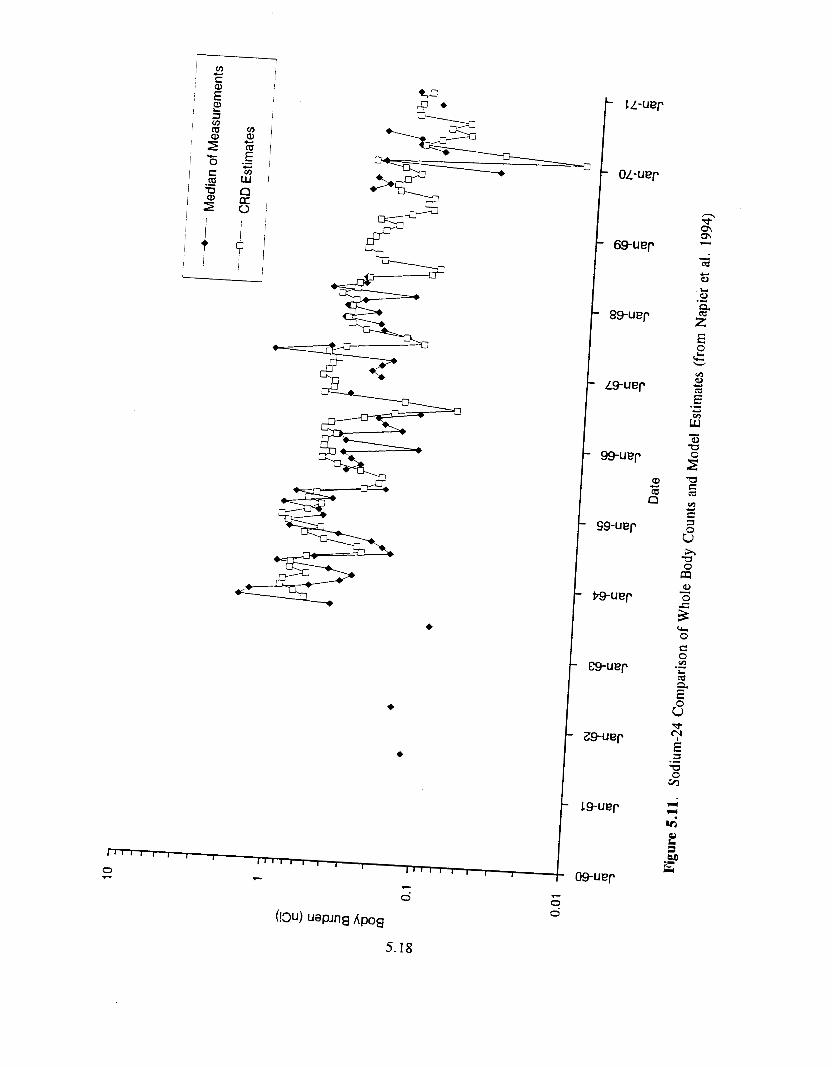
1 I
- sg-uer
0
m W Y
.- E" Y
E
a 2 r0Y Y c f
3 a 0 a
rc. 0 E 0
m m L .-
f" u" d c;' E 3 a 0 v)
.-
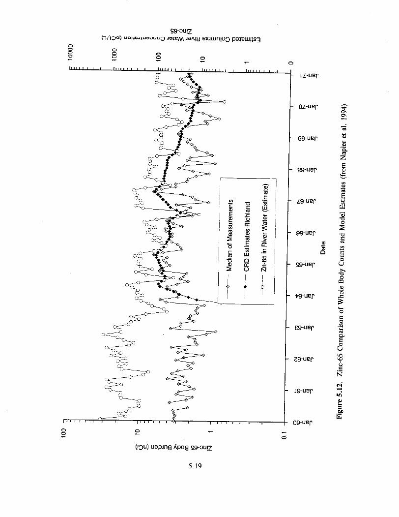
0 0 0 7
0 7
0 0 7
0 0 -
0
5.19

For use in validating the HEDR model, the course of the experiment was simulated as an individual ingesting 220 gramdweek of Richland whitefish (the average amount reported in the description of the experiment) in addition to 1 liter/day of treated Columbia River water. As shown in Section 4.2 (Table 4.4), these are the two most important exposure pathways for a maximum representative individual at Richland. The concentrations of zinc-65 in the whitefish were estimated using the bioconcentration factors derived for the HEDR Project. Body burden was estimated using the same uptake and retention parameters used by the ICRP in developing the ingestion dose factors used in the CRD code.
The results of the estimate are compared to the measurements (reported and in the Hanford database) in Figure 5.13. The estimated and measured lines are very similar and agreement could have been even better because the investigator's assimilation and retention of zinc-65 deviated signifi- cantly from the published ICRP values. This comparison indicates that if the ingestion rates of locally caught fish can be determined, the estimates of radiation dose should have very small biases.
I
1
1.
9
rn ). i . 4
v
t W
10000
U 0 m
i
1000 ' ,
N N N N 0 m FY FY
m -3
5J - 9 - 6 3
-3 5J z 8 7
9 - 5J a m 3
-3 z h
U
Date
Figure 5.13. Estimated and Measured Zinc45 Body Burden (from Napier et al. 1994)
5.20
6.0 Conclusions
Reliable and useful doses and their uncertainties have been reconstructed for possible exposures of representative individuals from historical releases of materials from the Hanford Site.
The most important means of exposure via the river pathway was consumption of resident fish.
The most important contributors to dose were zinc65 and phosphorus-32, respectively, released from the single-pass reactors.
The highest estimated dose was from resident fish caught in the Columbia River at Ringold, Washington, downstream of the Hanford reactors.
The highest estimated dose was to an adult consuming 40 kilograms (90 pounds) of resident fish from the Columbia River at Ringold, Washington (median dose of 140 millirem to the whole body for 1960).
The highest estimated dose to a typical adult was accumulated during the 1956-1965 time period with 1960 being the highest year (median dose of 5 millirem) at Pasco, Washington.
Doses for children for any specific year could be a factor of 1.5 to 2 higher than the adult doses for the typical representative individual.
The most important contributors to uncertainty in the dose estimates were the dose factor and the bioconcentration factors, respectively.
Representative individual doses included in this report allow individuals using the Columbia River commercially, for recreation, or as a source of water or foods to estimate their doses.
24 This report is the culmination of technical work performed to reconstruct doses that may have been received by persons who used the Columbia River from 1944 through 1992 for food, recreation, or commercial purposes. It summarizes the efforts to estimate 1) the quantity and timing of releases of radioactive materials to the river, 2) the transport, dilution, and decay of radioactive materials from the release points along the Columbia River to below Portland, Oregon, 3) the accumulation of radioactive materials in Columbia River water, fish, wateifowl, and oysters exposed to the Columbia River and adjacent ocean bays, and 4) the doses that representative individuals may have received from 1944-1992.
The HEDR Project staff have been able to identify and retrieve sufficient historical information to reconstruct, through computer modeling, the operational history of each of the eight Hanford single-pass production reactors. The results of this modeling along with recorded effluent monitoring and analytical data have been sufficient to quantify release of radioactive materials to the Columbia River. The modeling and historical measurements also have been adequate to identify and quantify the major sources of uncertainty both in the variability of parameters needed for calculations and in areas where information was missing.
6.1

Historical environmental measurements and the river transport code WSU-CHARIMA have been used to reconstruct the seasonal and dam-controlled flows of the Columbia River over the period of reactor operations, 1944- 197 1. Validation studies using environmental historical measurements have demonstrated the acceptability of using the computer codes to estimate radioactivity concentrations in the river for important times and locations.
The use of historical enviroqental measurements alone was inadequate for determining concentrations of radioactive materials in fish, waterfowl, and oysters affected by the Columbia River for times and locations of interest. However, the use of historical environmental measurements for fish along with concentrations of radioactive materials in the river water calculated by the WSU- CHARIMA code have been adequate to determine bioconcentration factors for fish for times and locations of interest. Historical environmental measurements for shellfish were adequate for dose estimating. There was sufficient information to quantify the variability of bioconcentration factors and to quantify the uncertainties of the historical measurements.
The reconstruction of concentrations of radioactive materials in Columbia River water, fish, waterfowl, and shellfish affected by the Columbia River and the determination of uncertainties in the estimates provide a sound basis for estimating doses that persons may have received from exposure to river media. Models and other parametric values necessary for estimating doses were summarized from open literature publications and have been peer-reviewed.
Results of independent testing of computer codes, statistical analyses of data, uncertainty analyses, sensitivity analyses, and validation studies demonstrate that the reconstruction of reactor operations, releases of radioactive materials to the river, transport of radioactive materials in the river, accumulation of radioactive materials in biota exposed to the Columbia River, and estimation of doses to representative individuals from use of the river and associated media are appropriate and fully meet HEDR Project objectives.
6.2

7.0 References
Baker, D.A., and W.T. Farris. 1994. User Instructions and Cofumbia River Dose (CRD) Computer Code. PNWD-2253 HEDR, Battelle, Pacific Northwest Laboratories, Richland, Washington.
Beetle, T.M. 1972. A Statistical Study of Radiation Damage for Fishermen. BNWL-SA-4449, Battelle Northwest Laboratory, Richland, Washington.
Brown, M.E., ed. 1957. The Physiology of Fishes, Volume A - Metabolism. Academic Press, New York.
Bramson, P.E., and J.P. Corley. 1973. Environmental Surveillance at Hanford for CY-1972. BNWL- 1727, Battelle Northwest Laboratory, Richland, Washington.
Denham, D.H., R.L. Dirkes, R.W. Hanf, T.M. Poston, M.E. Thiede, and R.K. Woodruff. 1993. Phase I Summaries of Radionuclide Concentration Data for Vegetation, River Water, Drinking Water, and Fish. PNWD-2 145 HEDR, Battelle, Pacific Northwest Laboratories, Richland, Washington.
DOE - U.S. Department of Energy. 1988. Internal Dose Conversion Factors for Calculation of Dose tu the Public. DOE/EH-0071, U.S. Department of Energy, Washington, DC.
Endres, G.W.R., J.K. Soldat, D.B. Shipler, N.M. Robinson, F.N. Eichner, and J.F. Honsted. 1972. Dietary and Body Burden Data and Dose Estimates for Local School Children and Teenagers. U.S. Environmental Protection Agency Research Report No. Y-80054-3, Battelle, Pacific Northwest Laboratories, Richland, Washington.
€PA - US. Environmental Protection Agency. 1988. Limiting Values of Radionuclide Intake and Air Concentrations and Dose Conversion Factors for Inhalation, Submersion, and Ingestion. Federal Guidance Report No. 11, EPA-520/1-88-020, Office of Radiation Programs, U.S. Environmental Protection Agency, Washington, DC. ’
EPA - U.S. Environmental Protection Agency. 1989. Exposure Factors Handbook. EPA/600//8- 89/043, Office of Health and Environmental Assessment, U.S. Environmental Protection Agency, Washington, DC.
Essig, T.H., and J.K. Soldat, eds. 1967. Evaluation of Radiological Conditions in the Vicini9 of Hanford for 1966. BNWL-439, Battelle Northwest Laboratory, Richland, Washington.
Essig, T.H., G.W. Endres, J.K. Soldat, and J.F. Honstead. 1973. Concentrations ofZn-65 in Marine Fuudstuffs and Pacific Coastal Residents. IAEA-SM-158/43, International Atomic Energy Agency, Vienna.
Farris, W.T. 1993. SofnYare Requirements Specifications for Columbia River Pathway: Source Term, River Transport, Environmental Accumulation and Dose Models. BN-SA-3799 HEDR, Battelle, Pacific Northwest Laboratones, Richland, Washington.
7.1
Fix. J.J. 1975. Environmental Surveillance at Hanfordfoi. CY-I 974. BNWL-1910, Battelle North- west Laboratory, Richland, Washington.
Fix. J.J.. P.J. Blumer, G.R. Hoenes, and P.E. Bramson. 1977. Environmental Surveillance at Hanford .fur CY-I 976. BNWL-2142, Battelle Northwest Laboratory, Richland, Waslungton.
Foerster, R.E. 1968. The Sockeye Salmon, Oncorhynchus nerka. Fisheries Research Board of Canada, Ottawa.
Foster, R.F., and J.F. Honstead. 1967. "Accumulation of Zinc-65 from Prolonged Consumption of Columbia River Fish." Health Physics 13( 1):39-43.
Foster, R.F., and K.H. Wilson. 1962. Evaluation of Radiological Conditions in the Vicinity of Hanford for 1961. HW-71999, General Electric Company, Hanford Atomic Products Operation, Richland, Washington.
Freshley, M.D., and P.D. Thome. 1992. Ground-Water Contribution tu Dose from Past Hanford Operations. PNWD- 1974 HEDR, Battelle, Pacific Northwest Laboratories, Richland, Washington.
Groves, L.R. 1962. Now it Can be Told: The Story of the Manhattan Project. Harbor and Brothers, New Yo&.
Hanf, R.W., R.L. Dirkes, and J.P. Duncan. 1992. Radioactive Contamination of Fish, Shellfish, and Waterfowl Exposed to Hanford Efluents: Annual Summaries, 1945-1 972. PNWD-1986 HEDR, Battelle, Pacific Northwest Laboratories, Richland, Washington.
Heeb, C.M., and D.J. Bates. 1994. Radionuclide Releases to the Columbia River from Hanford Operations, 1944-1 971. PNWD-2223 HEDR, Battelle, Pacific Northwest Laboratories, Richland, Waslungton.
Hoffman, F.O., W.J. Conover, M. Henrion, E. Hofer, and S. Simon 1993. Peer Review of HEDR Uncertainfy and Sensitiviry Analyses Plan. PNWD-2 162 HEDR, Battelle, Pacific Northwest Laboratories, Richland, Washington.
Holly, F.M., Jr., J.C. Yang, P. Schwaxz, J. Schaefer, S.H. Hsu, and R. Einhellig. 1993. CHARIMA-- Numerical Simulation of Unsteady Water and Sediment Movement in Multiple Connected Nenvorks of Mubilr-Bed Channels. IIHR Report No. 343, Iowa Institute of Hydraulic Research, University of Iowa, Iowa City, Iowa.
Houston, J.R., and P.J. Blumer. 1978. Environmental Surveillance at Hanford f o r CY-1977. PNL-26 14, Pacific Northwest Laboratory, Richland, Washington.
Houston, J.R., and P.J. Blumer. 1979. Environmental Surveillance at Hanford for CY-I 978. PNL-2932, Pacific Northwest Laboratory, Richland, Washington.
7.2

Houston, J.R., and P.J. Blumer. 1980. Environmental Surveillance at Hanford for CY-1979. PNL-3283, Pacific Northwest Laboratory, Richland. Washington.
ICRP - International Commission on Radiological Protection. 1977. Recommendations of the International Commission on Radiological Protection. ICRP Publication 26, Pergamon Press, New Y ork.
Jaquish, R E , and R.W. Bryce. 1989. Hanford Site Environmental Report for Calendar Year 1988. PNL-6825, Pacific Northwest Laboratory, Richland, Washington.
Jaquish, R.E., and R.W. Bryce. 1990. Hanford Site Environmental Report for Calendar Year 1989. PNL-7346, Pacific Northwest Laboratory, Richland, Washington.
Jaquish, R.E., and P.J. Mitchell. 1988. Environmental Monitoring at Hanford for 1987. PNL-6464, Pacific Northwest Laboratory, Richland, Washington.
Meehan, W.R. 1991. "Influences of Forest and Rangeland Management of Salmonid Fishes and Their Habitats." American Fisheries Society Special Publication 19:47-82.
Napier, B.A. 1991a. Computational Model Design Specification for Phase I of the Hanford Environ- mental Dose Reconstruction Project. PNL-7274 HEDR, Battelle, Pacific Northwest Laboratories, Richland, Washington.
Napier, B.A. 1991b. Selection of Dominant Radionuclides for Phase I of the Hanford Environmental Dose Reconstruction Project. PNL-723 1 HEDR, Pacific Northwest Laboratory, Richland, Washington.
Napier, B.A. 1993. Determination of Key Radionuclides and Parameters Related to Dosefrom the Columbia River Pathway. BN-SA-3768 HEDR, Battelle, Pacific Northwest Laboratories, Richland, Washington.
Napier, B.A., and A.J. Brothers. 1992. Recommendations to the Technical Steering Panel Regarding Approach for Estimating Individual Radiation Doses Resulting from Releases of Radionuclides to the Coliimbia River, Volume 1: Recommendations. PNWD-!977 HEDR, Vol. 1, Battelle, Pacific North- west Laboratories, Richland, Washington.
Napier, B.A., J.C. Simpson, P.W. Eslinger, J.V. Ramsdell, Jr., M.E. Thiede, and W.H. Walters. 1994. Validation of HEDR Models. PNWD-222 1 HEDR, Battelle, Pacific Northwest Laboratories, Richland, Washington.
NCRP - National Council on Radiation Protection and Measurements. 1984. Radiological Assessment: Predicting the Transport, Bioconcentration, and Uptake by Man of Radionuclides Released to the Environment. NCRP Report No. 76, National Council on Radiation Protection and Measurements, Bethesda, Maryland.
7.3

Oregon Department of Hsb & Wildlife and Washington Department of Fisheries. 1993. Status R q o r r , Columbia River Fish Runs and Fisheries 1938-92. Washington Department of Fisheries, Olympia, Washington
Parker. H.M., and W.D. Norwood. 1946a H.I. Section Report for October f946. HW-7-5301, General Electric Company, Hanford Works, Richland, Washington.
Parker. H.M., and W-D. Norwood. 1946b. H.I. Section Repon for November 1946. HW-7-5428, General Electric Company, Hanford Works, Richland, Washington.
Phipps, A.W., G.M. Kmdall, J.W. Stather, and T.P. Fell. 1991. Committed Equivalent Organ Doses and Committed Effeaive Doses from Intakes of Radionuclides. NRPB-R245, National Radiological Protection Board. Chilmn, Didcot, United Kingdom.
PNL - Pacific No~thwm Lahoratory. 1987. Environmental Monitoring at Hanford for 1986. PNL-6 120. Pacific Northwest Laboratory, Richland, Washington.
PNL - Pacific No&avest Laboratory. 1991. Columbia River Pathway Report: Phase f of the Hanford Enviromwmal Dose Reconstruction Project. PNL-7411 HEDR Rev. I , Pacific Northwest Laboratory. RicNarsd Washington.
Poston. T.M., and DE. Klopfer. 1988. "Concentration Factors Used in the Assessment of Radiation Dose to Consumers of Fish: A Review of 27 Radionuclides." Health Physics 55(5):751-766.
Shipler, D.B. 1993. Integrated Task Plans for the Hanford Dose Reconstruction Project, June 1992 Through M e 1994. PNWD-2187 HEDR, Battelle, Pacific Northwest Laboratories, Richland, Washington.
Shipler. D.B., and B-A Napier. 1992. HEDR Modeling Approach. PNWD-1983 HEDR, Battelle. Pacific Northwest Ubomories, RicNand, Washington.
Shipler, D.B.. and B.A. Napier. 1994. HEDR Modeling Approach. PNWD-1983 HEDR Rev. 1, Battelle, Pacific N W & Laboratories, Richland, Washington.
Simpson. J.C., and J.V. Ramsdell. Jr. 1993. Uncertain0 and Sensitivity Analyses Plan. PNWD-2124 HEDR, Battelle, Pacific Northwest Laboratories, Richland, Washington.
Snyder. S.F.. W.T. Farris, B.A. Napier, T.A. Ikenbeny, and R.O. Gilbert. 1994. Parameters Used in the Environmental Pafhways and Radiological Dose Modules (DESCARTES, CIDER, and CRD Codes) of the Hanford Environmental Dose Reconstruction Integrated Codes (HEDRIC). PNWD-2023 HEDR Rev. 1. Battelle, Pacific Northwest Laboratories, Richland, Washington.
7.4

Soldat, J.K. 1968. A Statistical Study of the Habits of Fishermen Utilizing the Columbia River Below Hanford. BNWL-SA- 145 1, Battelle Northwest Laboratory, Richland, Washington.
Soldat, J.K. 1989. Ofsite Radiation Doses from Hanford Operations for the Years 1983 through 1987: A Comparison of Results Calculated by Two Methods. PNL-7 135, Pacific Northwest Laboratory, Richland, Washington.
Soldat, J.K., and T.H. Essig, eds. 1966. Evaluation of Radiological Conditions in the Vicinity of Hanford for 1965. BNWL-3 16, Battelle Northwest Laboratory, Richland, Washington.
Soldat, J.K.. and J.F. Honstead. 1968. Dietary Levels for Tri-City Elementary School Children. BNWL-CC- 1565 (February 26, 1968), Battelle Northwest Laboratory, Richland, Washington.
Soldat. J.K., K. R. Price, and W.D. McCormack. 1986. Off-Site Radiation Doses Summarized from Hanford Environmental Monitoring Reports for the Years 1957-1 984. PNL-5795, Pacific Northwest Laboratory, Richland, Washington.
Spear, D.R., J.J. Fix, and P.J. Blumer. 1976. Environmental Surveillance at Hanford for CY-197.5. BNWL- 1979, Battelle Northwest Laboratory, Richland, Washington.
Sula, M.J., and P.J. Blumer. 1981. Environmental Surveillance at Hanford for CY-1980. PNL-3728, Pacific Northwest Laboratory, Ri chl and, Washington.
Sula, M.J., J.M.V. Carlile, K.R. Price, and W.D. McCormack. 1983. Environmental Surveillance at Hanford for CY-1982. PNL-4657, Pacific Northwest Laboratory, Richland, Washington.
Sula, M.J., W.D. McCormack, R.L. Dirkes, K.R. Price, and P.A. Eddy. 1982. Environmental Surveil- lance at Hanford for CY-1981. PNL-42 1 1, Pacific Northwest Laboratory, Richland, Washington.
Swanberg, F., Jr. 1962. "Quantitative Measurements of Some Gamma-Ray-Emitting Radionuclides in Nuclear Industrial Workers by Whole-Body Counting Techniques." Health Physics 8( 1):67-7 1 .
Thlede, M.E., D. J. Bates, E.I. Mart, and R. W. Hanf. 1994. A Guide to Environmental Monitoring Data, 1945 through 1972. PNWD-2226 HEDR, Battelle, Pacific Northwest Laboratories, Richland, W ashmgton.
Vanderploeg, H.A., D.C. Parzyck, W.H. Wilcox, J.R. Keruher, and S.V. Kaye. 1975. Bioaccumula- tion for Radionuclides in Freshwater Biota. ORNL-5002, Oak Ridge National Laboratory, Oak Ridge, Tennessee.
Walters, W.H., R.L. Dirkes, and B.A. Napier. 1992. Literature and Data Review for the Sulface- Water Pathway: Columbia River and Adjacent Coastal Areas. PNWD-2034 HEDR, Battelle, Pacific Northwest Laboratories, Richland, Washington.
7.5

Walters, W.H., M.C. Richmond, and B.G. Gilmore. 1994. Reconstruction of Radionuclide Concentra- tions in the Columbia River from Hanford, Washington, to Portland, Oregon, January 1950-January 1971. PNWD-2225 HEDR, Battelle, Pacific Northwest Laboratories, Richland, Washington. '
Woodruff, R.K., and R.W. Hanf. 1991. Hanford Site Environmental Report for Calendar Year 1990. PNL-7930, Pacific Northwest Laboratory, Richland, Washington.
Woodruff, R.K., and R.W. Hanf. 1992. Hanford Site Environmental Report for Calendar Year 1991. PNL-8 148, Pacific Northwest Laboratory, Richland, Washington.
Woodruff, R.K., and R.W. Hanf. 1993. Hanford Site Environmental Report for Calendar Year 1992. PNL-8682, Pacific Northwest Laboratory, Richland, Washington.
7.6

Appendix A
Summary of Estimated Columbia River Doses

Appendix A
Summary of Estimated Columbia River Doses
The doses to the three different representative individual types are presented in this appendix. The parameters that describe the representative individuals are presented in Section 3.4.3. The doses are presented as dose equivalent for red bone marrow and lower large intestine and as effective dose equivalent. All doses are in units of millirem for the effective dose equivalent. Both monthly esti- mates for each of 253 months and annual totals are provided for the period 1950 through 1971. For the red bone marrow and lower large intestine, doses estimated are presented as annual totals. Doses are calculated for twelve specific river segments. The segment names and approximate locations are as follows:
1. 2. 3. 4. 5. 6. 7. 8. 9. 10. 11. 12.
Ringold (from below reactor areas to north of Richland) Richland (from north of Richland to above the Yakima River) KennewickPasco (from below the Yakima River to the Snake River) Snake/Walla Walla rivers (from below the Snake River to near McNary Dam) UmatiWBoardrnan (from near McNary Dam to near Arlington, Oregon) Arlington (Arlington, Oregon vicinity) John Day DandBiggs (from below Arlington, Oregon, to near Biggs, Oregon) Deschutes River (Deschutes River mouth vicinity) The Dalles/Celilo (The Dalles/Celilo vicinity) Klickitat River (Klickitat River mouth vicinity) White SalmodCascade Locks (from White Salmon River to Bonneville Dam) Lower River (from below Bonneville Dam to Columbia River mouth)
A. 1

Table A.1. Maximum Representative Individual - Effective Dose Equivalent (millirem per month and millirem per year)
Month/Y ear
Cum. Dose J AN50 FEB5O MAR50 APRSO MAY50 JUN5O JULSO AUG5O SEPSO Ocr50 NOV50 DEC5O
1950
JAN51 FEB5 1 MAR51 APR51 MAY5 1 JUN5 1 JUL5 1 AUGS 1 SEP5 1 om5 I NOV5 1 DECS 1
1951
JAN52 FEB52 MARS2 APR52 MAY52 JUN52 JUL52 AUG52 SEP52 Om52 NOV52 DEC52
1952
JAN53 FEBS3 MAR53 APE3 MAY53 JUN53 JUL53 AUG53 SEP53 Om53 NOV53 DEC53
1
1420 4.4
4 2.4 1.7
0.91 0.86 0.99 2.3 3.8
5 6.9 4.3 38
2.4 2
1.7 1.1
0.42 0.91
1.1 2.5 4.8 3.8 5.4 2.8 29
3.4 2.5 1.9 1.4
0.57 0.86
1.6 2.2 4.3
8 9.2 6.9 43
7.8 4.5 2.5 1.5 1.6 1.1 1.6 3.9 4.8 5.8 10 6
2
1400 4.1 3.7 2.1 1.5
0.83 0.83 0.95 2.2 3.6 4.8 6.6 4.1 35
2.3 1.9 1.5
1 0.38 0.87
1.1 2.4 4.6 3.6 5.2 2.7 28
3.2 2.3 1.6 1.2
0.52 0.82
1.5 2.1 4.2 7.7 8.9 6.5 40
7.4 4.3 2.2 1.4 1.5
1 1.5 3.7 4.5 5.5 9.5 5.6
3
1300 4.3 3.8 2.2 1.6
0.92 0.85 0.99 2.3 3.7 4.8 6.4
4 36
2.3 1.9 1.6 1.1
0.43 0.9 1.1 2.4 4.7 3.7 5.3 2.8 28
3.4 2.4 1.8 1.3
0.59 0.86
1.6 2.1 4.2 7.1 8.8 6.7 41
7.1 4.2 2.4 1.5 1.6 1.1 1.5 3.8 4.6 5.6 9.1 5.5
4
880 3
2.4 1.2
0.84 0.58 0.6
0.85 1.9 2.9 3.4 4.3 2.7 25
1.7 1.2
0.98 0.58 0.29 0.7
1 2
3.7 2.7 3.6 1.9 20
2.5 1.5 1.1
0.52 0.32 0.6 1.3 1.7 3.1 5.5 6.4 4.8 29
4.1 2.7 1.5
0.87 0.83 0.71
1.2 3.1 3.7 4.3 6.4 3.7
5
709 2.9 2.3 1.1
0.78 0.53 0.59 0.81
1.8 2.7 3.2 4.2 2.6 23
1.6 1.1
0.86 0.53 0.27 0.67 0.95
1.9 3.5 2.6 3.5 1.8 19
2.3 1.4
0.97 0.46 0.29 0.57
1.2 1.6 2.9 5.2 6.1 4.6 28
3.8 2.5 1.3
0.74 0.72 0.68
1.1 2.8 3.4
4 4.7 2.7
A.2
Location 6
684 2.7 2.2
1 0.72 0.5
0.58 0.78
1.7 2.6 3.1
4 2.5 22
1.5 1.1
0.77 0.49 0.25 0.64 0.91
1.8 3.3 2.5 3.4 1.7 18
2.2 1.4
0.87 0.42 0.27 0.55
1.1 1.5 2.7 4.9 5.9 4.3 26
3.6 2.4 1.2
0.64 0.63 0.65
1.1 2.6 3.1 3.8 4.6 2.7
7
666 2.6 2.1
0.94 0.67 0.48 0.56 0.76
1.6 2.5
3 3.9 2.4 22
1.4 1
0.71 0.45 0.24 0.62 0.88
1.8 3.2 2.4 3.3 1.7 18
2.1 1.3
0.81 0.38 0.25 0.53
1.1 1 .5 2.6
' 4.8 5.7 4.2 25
3.4 2.2 1.1
0.58 0.57 0.63
1 2.5
3 3.6 4.5 2.6
8
629 2.5
2 0.89 ,0.65 0.46 0.56 0.75
1.6 2.4 2.9 3.7 2.3 21
1.3 0.95 0.67 0.43 0.24 0.61 0.87
1.7 3.1 2.3 3.1 1.6 17
2 1.2
0.76 0.37 0.25 0.52
1.1 1.4 2.5 4.5 5.4 3.9 24
3.1 2.1
1 0.55 0.55 0.62
1 2.4 2.8 3.5 4.2 2.4
9
618 2.5
2 0.87 0.64 0.46 0.55 0.74
1.6 2.4 2.9 3.7 2.3 20
1.3 0.94 0.65 0.42 0.23 0.61 0.86
1.7 3
2.3 3.1 1.6 17
2 1.2
0.75 0.36 0.24 0.52
1.1 1.4 2.5 4.5 5.3 3.9 24
3.1 2.1
0.98 0.53 0.53 0.61 0.99 2.3 2.8 3.4 4.2 2.4
10
597 2.3 1.9
0.81 0.61 0.44 0.54 0.73
1.5 2.3 2.8 3.5 2.2 20
1.3 0.9
0.61 0.4
0.22 0.59 0.84
1.6 2.9 2.2
3 1.5 16
1.9 1.2
0.69 0.34 0.23 0.51
1 1.4 2.3 4.2 5.1 3.7 23
2.8 2
0.9 0.49 0.5
0.59 0.97 2.2 2.6 3.2
4 2.3
11
576 2.1 1.8
0.75 0.57 0.41 0.53 0.7 1.5 2.2 2.6 3.4 2.1 19
1.2 0.86 0.55 0.38 0.21 0.58 0.82
1.5 2.7 2.2 2.9 1.4 15
1.8 1.1
0.63 0.3 1 0.22 0.49 0.97
1.3 2.2 3.9 4.9 3.4 21
2.5 1.9
0.81 0.44 0.45 0.58 0.92 2.1 2.5 3.1 3.9 2.2
12
456 1.6 1.4
0.45 0.46 0.32 0.48 0.61
1.1 1.7 1.3 1.9 1.9 15
0.71 0.59 0.37 0.3
0.18 0.53 0.74
1.3 2.3 1.7 2.1
0.83 12
1.2 0.7
0.42 0.24 0.18 0.44 0.84
1.1 1.7
3 5.4 2.9
18
0.98 1.1
0.53 0.3 1 0.32 0.51 0.8 1.7
2 2.4
1.1 2.7
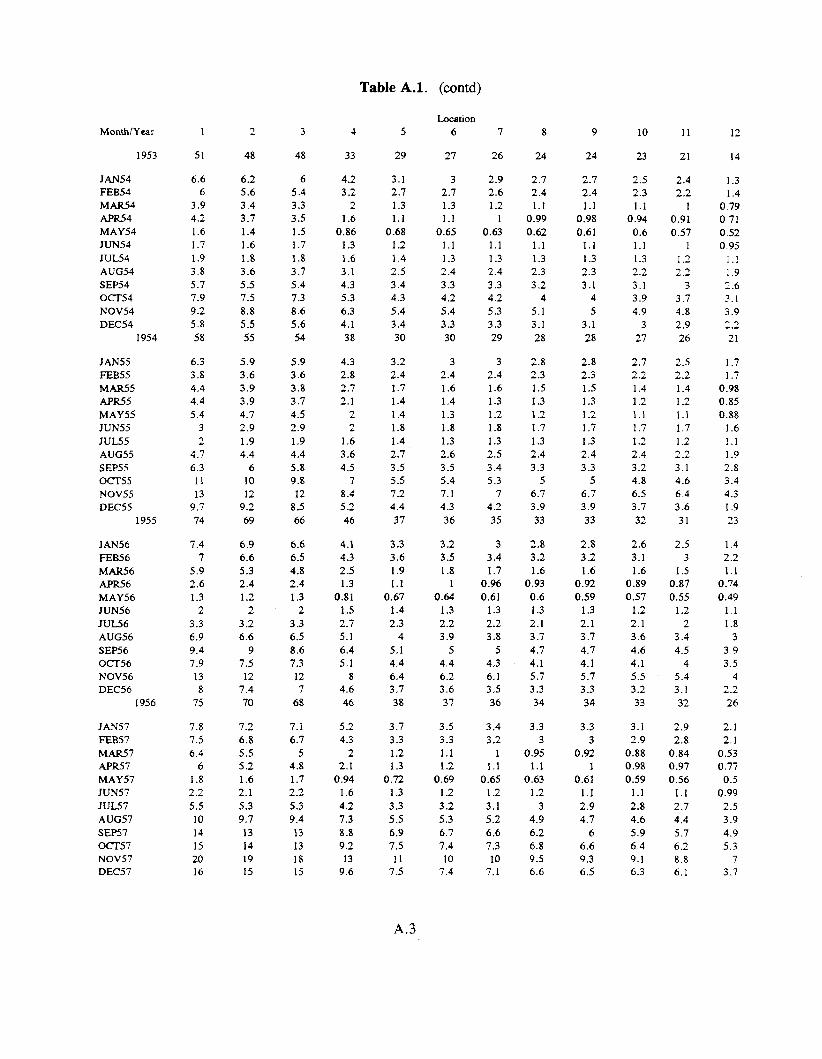
Table A.l. (contd)
Location 6
27
3 2.7 1.3 1.1
0.65 1.1 1.3 2.4 3.3 4.2 5.4 3.3 30
3 2.4 1.6 1.4 1.3 1.8 1.3 2.6 3.5 5.4 7.1 4.3 36
3.2 3.5 1.8
1 0.64
1.3 2.2 3.9
5 4.4 6.2 3.6 37
3.5 3.3 1.1 1.2
0.69 1.2 3.2 5.3 6.7 7.4 10
7.4
MonthlYear
1953
JAN54 FEB54 MAR54 APR54 MAY54 JUN54 JUL54 AUG54 SEP54 0'354 NOV54 DEC54
1954
JAN55 FEB55 MAR55 APR55 MAY55 JUN55 JUL55 AUG55 SEP55 O a 5 5 NOV55 DEC55
1955
JAN56 FJZB56 MAR56 APE6 MAY56 JUN56 JUL56 AUG56 SEP56 0'356 NOV56 DEC56
1956
JAN57 FEB57 MAR57 APR57 MAY57 JUN57 JUL57 AUG57 SEP57 ocT57 NOV57 DEC57
1
51
6.6 6
3.9 4.2 1.6 1.7 1.9 3.8 5.7 7.9 9.2 5.8 58
6.3 3.8 4.4 4.4 5.4
3 2
4.7 6.3 11 13
9.7 74
7.4 7
5.9 2.6 1.3
2 3.3 6.9 9.4 7.9 13 8
75
7.8 7.5 6.4
6 1.8 2.2 5.5 10 14 15 20 16
2
48
6.2 5.6 3.4 3.7 1.4 1.6 1.8 3.6 5.5 7.5 8.8 5.5 55
5.9 3.6 3.9 3.9 4.7 2.9 1.9 4.4
6 10 12
9.2 69
6.9 6.6 5.3 2.4 1.2
2 3.2 6.6
9 7.5 12
7.4 70
7.2 6.8 5.5 5 2 1.6 2.1 5.3 9.7 13 14 19 15
3
48
6 5.4 3.3 3.5 1.5 1.7 1.8 3.7 5.4 7.3 8.6 5.6 54
5.9 3.6 3.8 3.7 4.5 2.9 1.9 4.4 5.8 9.8 12
8.5 66
6.6 6.5 4.8 2.4 1.3
2 3.3 6.5 8.6 7.3 12 7
68
7. 1 6.7
5 4.8 1.7 2.2 5.3 9.4 13 13 18 15
4
33
4.2 3.2
2 1.6
0.86 1.3 1.6 3.1 4.3 5.3 6.3 4.1 38
4.3 2.8 2.7 2.1
2 2
1.6 3.6 4.5
7 8.4 5.2 46
4.1 4.3 2.5 1.3
0.81 1.5 2.7 5.1 6.4 5.1
8 4.6 46
5.2 4.3
2 2.1
0.94 1.6 4.2 7.3 8.8 9.2 13
9.6
5
29
3.1 2.7 1.3 1.1
0.68 1.2 1.4 2.5 3.4 4.3 5.4 3.4 30
3.2 2.4 1.7 1.4 1.4 1.8 1.4. 2.7 3.5 5.5 7.2 4.4 37
3.3 3.6 1.9 1.1
0.67 1.4 2.3
4 5.1 4.4 6.4 3.7 38
3.7 3.3 1.2 1.3
0.72 1.3 3.3 5.5 6.9 7.5 11
7.5
A.3
7
26
2.9 2.6 1.2
1 0.63
1.1 1.3 2.4 3.3 4.2 5.3 3.3 29
3 2.4 1.6 1.3 1.2 1.8 1.3 2.5 3.4 5.3
7 4.2 35
3 3.4 1.7
0.96 0.61
1.3 2.2 3.8
5 4.3 6.1 3.5 36
3.4 3.2
1 1.1
0.65 1.2 3.1 5.2 6.6 7.3 10
7.1
8
24
2.7 2.4 1.1
0.99 0.62
1.1 1.3 2.3 3.2
4 5.1 3.1 28
2.8 2.3 1.5 1.3 1.2 1.7 1.3 2.4 3.3
5 6.7 3.9 33
2.8 3.2 1.6
0.93 0.6 1.3 2.1 3.7 4.7 4.1 5.7 3.3 34
3.3 3
0.95 1.1
0.63 1.2
3 4.9 6.2 6.8 9.5 6.6
9
24
2.7 2.4 1.1
0.98 0.61
1.1 1.3 2.3 3.1
4 5
3.1 28
2.8 2.3 1.5 1.3 1.2 1.7 1.3 2.4 3.3
5 6.7 3.9 33
2.8 3.2 1.6
0.92 0.59
1.3 2.1 3.7 4.7 4.1 5.7 3.3 34
3.3 3
0.92 1
0.61 1.1 2.9 4.7
6 6.6 9.3 6.5
10
23
2.5 2.3 1.1
0.94 0.6 1.1 1.3 2.2 3.1 3.9 4.9
3 27
2.7 2.2 1.4 1.2 1.1 1.7 1.2 2.4 3.2 4.8 6.5 3.7 32
2.6 3.1 1.6
0.89 0.57
1.2 2.1 3.6 4.6 4.1 5.5 3.2 33
3.1 2.9
0.88 0.98 0.59
1.1 2.8 4.6 5.9 6.4 9.1 6.3
11
21
2.4 2.2
1 0.91 0.57
1 1.2 2.2
3 3.7 4.8 2.9 26
2.5 2.2 1.4 1.2 1.1 1.7 1.2 2.2 3.1 4.6 6.4 3.6 31
2.5 3
1.5 0.87 0.55
1.2 2
3.4 4.5
4 5.4 3.1 32
2.9 2.8
0.84 0.97 0.56
1.1 2.7 4.4 5.7 6.2 8.8 6.1
12
14
1.3 1.4
0.79 0.71 0.52 0.95
1.1 1.9 7.6 3.1 3.9 2.2 21
1.7 1.7
0.98 0.85 0.88
1.6 1.1 1.9 2.8 3.4 4.3 1.9 23
1.4 2.2 1 . 1
0.74 0.49
1 . 1 1.8
3 3.9 3-5
4 2.2 26
2.1 2.1
0.53 0.77 0.5
0.99 2.5 3.9 4.9 5.3
7 3.7

Table A.l . (contd)
Location 6
51
4.6 4.6 1.4 1.8
1 1.8 4.5 5.5 4.6 7.5 8.8 4.8 51
3.3 3.9 1.7 1.3
0.84 1.4 2.1 3.3 5.7 4.5 9.4 5.9 43
11 5.2 2.1 1.6 1.4 2.8 3.4 3.9 6.4 7.1 11
8.5 64
9.3 6.6 3.4 3.8 1.7 2.5 2.4 5.3 6.5 6.2 8.9 4.3
Month/Year
1957
JAN58 FEB58 MAR58 AFR58 MAY58 JUN58 JUL58 AUG58 SEP58 Om58 NOV58 DEC58
1958
JAN59 FEB59 MAR59 ApR59 MAY59 JUN59 NL59 AUG59 SEP59 Om59 NOV59 DEC59
1959
JAN60 FEW MAR60 APR60 MAY60 JUN60 JUL60 AUG60 S E W OCT60 NOV60 DEC60
1960
JAN61 FEB6 1 MAR61 APR6 1 MAY61 JUN61 JUL61 AUG61 SEP61 OCT6 1 NOV61 DEC61
1
110
13 12 6
6.9 3 3
8.1 11 10 17 20 12
1 20
8.8 9.5 5.9 4.3 2.1 2.3 3.1 6.4 9.5 8.4 17 11 89
22 9.3 8.6 4.6 3.6 4.6 4.9 8.2 13 14 24 19
140
23 13
9.4 8.7 3.4 3.4 3.7 8.8 12 11 18
8.2
2
110
12 11
5.3 6.2 2.8
3 7.8 10
9.9 16 19 11
110
8.4 8.9 5.4
4 2
2.3 3.1 6.4 9.4 8.2 17 11 86
21 8.9 7.8 4.4 3.6 4.6 4.9
8 13 14 23 18
130
22 12
8.9 8.3 3.4 3.4 3.7 8.7 12 11 17 8
3
100
11 10
4.7 5.8 2.8
3 7.7 9.9
9 15 17 11
110
7.6 8.2 4.8 3.8
2 2.3 3.1
6 9
7.9 16 10 81
20 8.4 6.7 4.2 3.4 4.6 4.8 7.4 12 13 21 17
120
20 12
7.9 7.8 3.2 3.4 3.6 8.3 11 10 16
7.4
4
68
7.3 5.6 2.7 2.9 1.5 2.2 6.2 7.7 6.2 10 11
6.2 70
4.7 5.3
3 2.1 1.3 1.7 2.7 4.8
7 5.5 11
7.3 57
14 5.6 3.5 2.7 2.1 3.3 4.2 5.7 8.6 9.2 14 11 85
13 7.3 4.9 4.9 2.1 2.8 3.1 6.8
8 7.1 11
4.9
5
53
4.8 4.6 1.5 1.9 1 .I 1.8 4.7 5.6 4.7 7.7
9 4.9 52
3.4 4
1.8 1.4 0.9 1.5 2.2 3.4 5.8 4.6 9.7 6.1 45
11 5.2 2.2 1.7 15 2.9 3.5
4 6.6 7.3 11
8.8 66
9.7 6.6 3.5 3.9 1.7 2.6 2.5 5.5 6.6 6.2 9.2 4.3
A.4
7
50
4.4 4.3 1.3 1.7
0.97 1.7 4.3 5.4 4.6 7.3 8.7 4.7 49
3.1 3.8 1.6 1.3 0.8 1.4 2.1
5.6 4.4 9.2 5.8 42
10 5.2
2 1.6 1.4 2.7 3.4 3.8 6.3
7 11
8.3 63
9.1 6.4 3.2 3.7 1.6 2.5 2.4 5.3 6.4 6.1 8.7 4.2
3.3
8
47
3.9 3.9 1.2 1.6
0.93 1.7 4.1 5.1 4.3 6.8 8.1 4.4 46
2.9 3.5 1.5 1.2
0.77 1.4 2.1 3.1 5.4 4.2 8.8 5.5 40
9.6 5
1.9 1.5 1.3 2.7 3.3 3.7 5.9 6.5 10
7.6 59
8.3 6.1
3 3.5 1.6 2.4 2.3
5 6
5.7 8
3.9
9
46
3.7 3.9 1.2 1.6
0.91 1.6
4 5
4.2 6.5
8 4.3 45
2.8 3.4 1.5 1.2
0.74 1.4
2 3
5.3 4.2 8.6 5.4 39
9.2 5
1.8 1.4 1.3 2.7 3.2 3.6 5.8 6.3 9.8 7.4 58
7.9 6 3
3.4 1.6 2.4 2.3 4.9 5.9 5.7 7.8 3.9
10
45
3.4 3.7 1.1 1.5
0.87 1.6 3.9 4.8 4.1 6.3 7.8 4.1 43
2.6 3.3 1.4 1.1 0.72
1.3 2
2.9 5.2 4.1 8.3 5.3 38
8.8 5.1 1.8 1.4 1.3 2.6 3.2 3.5 5.6 6.1 9.4 7.1 56
7.4 5.9 2.8 3.4 1.6 2.4 2.3 4.7 5.7 5.6 7.5 3.8
11
43
3.2 3.6 1.1 1.5
0.84 1.5 3.7 4.7
4 6
7.6 4
42
2.5 3.1 1.4 1.1
0.69 1.3 1.9 2.9
5 4
8.1 5.2 37
8.3 5.1 1.7 1.3 1.2 2.6 3.1 3.4 5.3
6 9.1 6.8 54
6.9 5.7 2.7 3.3 1.6 2.3 2.2 4.5 5.6 5.5 7.2 3.8
12
34
1.6 2.2
0.82 1.2
0 76 1.4 3.2 4.1 3.5 4.7 5.4 2.9 32
1.6 2.1 1.1
0.94 0.6 1.2 1.8 2.5 4.4 3.5 6.5 4.2 30
5.8 3.8 1.2 1.1
1 2.3 2 9
3 4 4
5 5 9 4 4 41
4.3 3.9 1.8 2.7 1.5 2.2 2.1 3.8
5 5.1 5.2 2.5

Table A.l . (contd)
Location Month/Yenr
1961
JAN62 FEB62 MAR62 APR62 MAY62 JUN62 JUL62 AUG62 SEP62 Om62 N OV62 DEC62
1962
JAN63 FEB63 MAR63 APR63 MAY63 JUN63 JUL63 AUG63 SEP63 Om63 NOV63 DEC63
1963
JAN64 FEB64 MAR64 APR64 MAY64 JUN64 JUL64 AUG64 SEP64 Om64 NOV64 DEC64
1964
JAN65 FEB65 MAR65 APR65 MAY65 JUN65 JUL65 AUG65 SEP65 Om65 NOV65 DEC65
1
120
13 8.9 8.2 8.6 3.2 5.1 7.4 12 22 11 14
9.9 120
6.5 5.2 4.5 4.1 2.1 2.4
3 5
6.9 8.7 12
7.1 68
8.2 6.3 5.1 5.4 3.3 2.1 1.8 4.2 8.1 4.7 11
6.5 67
6.4 4.3 3.4 3.1 1.5 2.1
2 3.5 5.9 8.2 8.2 4.7
2
120
13 8.7 7.5 8.2 3.2 5.2 7.4 12 22 11 14
9.7 120
6.4 5.1 4.2
4 2.1 2.4
3 4.9 7.3 9.2 13
7.7 72
8.6 6.7 5.4 5.9 3.8 2.3
2 4.5 8.6 5.1 12
7.1 72
6.8 4.7 3.8 3.4 1.8 2.3 2.2 3.7 6.2 8.3 8.6
5
3
110
12 8.1 6.5 7.6 3.2 5.1 7.4 11 21 11 13
9.1 120
6 4.7 3.5 3.6
2 2.3 2.9 4.5
6 7.7 11
6.3 60
7 5 .I 3.9 4.4 3.1 2.1 1.8
4 7.2 4.4 9.9 5.6 59
5.4 3.8 2.9 2.7 1 .5 2.1
2 3.2 5.1 6.7 7.3 4.2
4
77
7.7 5.2 3.6 3.8 1.9 3.7 6.2 9.2 16
7.3 8.7
6 79
4.4 2.8
2 2.1
1 1.6 2.3 3.5 4.1 5.3
7 4 40
4.4 3.9 2.3 1.9 1.5 1.4 1.4
3 4.9 3.2 6.7 3.1 38
3.1 1.9 1.5 1.3
0.87 1.4 1.5 2.4 3.4 4.1 4.9 2.8
5
62
5.8 4.6 2.6 2.9 1.5 3.3 5.5 7.8 13
7.7 7.7 5.2 68
3.4 2.6 1.1 1.4
0.71 1.3 1.7 2.4
3 3.9 5.5 3.1 30
2.9 3.1 1.3 1.3
1 1.2
1 2.2 3.7 2.6 5.1 2.4 28
2.4 1.6
1 0.93 0.6 1.2 1.1 1 .I 2.4
3 3.8 2.2
A.5
6
61
5.6 4.6 2.5 2.9 1.5 3.2 5.4 7.6 13
7.8 7.6 5.1 67
3.3 2.5
1 1.3
0.68 1.3 1.6 2.4 2.9 3.8 5.4
3 29
2.8 3
1.3 1.3
0.98 1 2
0.99 2.1 3.6 2.6
5 2.4 27
2.4 1.6
0.96 0.9
0.55 1.2 1.1 1.6 2.3 2.9 3.7 2.i
7
60
5.5 4.5 2.4 2.7 1.4 3.2 5.3 7.6 13
7.9 7.5
5 66
3.2 2.4
0.98 1.2
0.65 1.2 1.6 2.3 2.9 3.7 5.3 2.9 28
2.7 2.9 1.3 1 2
0.94 1.1
0.95 2.1 3.6 2.5 4.9 2.3 26
2.2 1.5
0.92 0.86 0.52
1.1 1.1 1.6 2.3 2.8 3.7 2.1
8
56
5.1 4.2 2.3 2.6 1.4 3.1 5.2 7.2 12
7.6 7
4.7 62
3 2.3
0.91 1.2
0.62 1.2 1.5 2.2 2.7 3.4 4.8 2.7 26
2.5 2.8 1.2 1.1
0.91 1.1
0.93 2
3.4 2.5 4.6 2.1 25
2.1 1.4
0.88 0.82 0.5 1.1
1 1.5 2.2 2.6 3.5 1.9
9
55
4.9 4.2 2.2 2.6 1.4 3.1 5.1 7.1 12
7.8 6.9 4.6 61
2.9 2.3
0.88 1.2
0.61 1.2 1.5 2.1 2.6 3.2 4.7 2.6 26
2.3 2.7 1.2 1.1
0.88 1.1
0.91 1.9 3.3 2.4 4.4 2.1 24
2 1.4
0.85 0.81 0.49
1.1 1
1.5 2.1 2.5 3.3 1.9
10
53
4.7 4.2 2.2 2.4 1.4
3 5 7
11 7.8 6.7 4.5 60
2.8 2.2
0.85 1.1 0.6 1.2 1.4 2.1 2.5 3.1 4.5 2.5 25
2.2 2.6 1.1 1.1
0.85 1.1
0.88 1.9 3.1 2.4 4.1
2 23
1.9 1.4
0.83 0.79 0.47
1.1 0.98
1.4 2
2.4 3.2 1.8
11
51
4.5 4.1 2.1 2.5 1.3
3 4.9 6.8
11 7.9 6.6 4.4 59
2.7 2.2
0.82 1.1
0.59 1.1 1.4
2 2.4 2.9 4.4 2.4 24
2 2.5 1.1 1.1
0.82 1.1
0.85 1.8
3 2.4 3.9
2 22
1.8 1.3
0.79 0.77 0.44
1.1 0.95
1.4 1.9 2.3
3 1.7
12
40
3.3 3.4 1.5
2 1.2 2.8 4.5 6.1 9.3
7 4.8 3.2 49
2.2 1.7
0.65 0.77 0.5
1 1.2 1.7
2 2.8
4 1.7 20
0.93 1.8
0.76 0.89 0.71
1 0.77
1.6 3
2 2 2.8 1.1 18
1.1 1.1
0.67 0.7
0.39 1
0.88 1.2 1.6 1.9 2.5 1.3
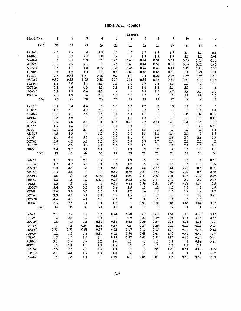
Table A.l. (contd)
Location 6
21
1.7 1.4
0.66 0.63 0.48 0.87 0.3
0.36 2.7 3.7
4 2.2 19
2.2 2.2 1.1 1.2
0.73 1 .I 1.4 2.4 3.1 2.9 3.2 1.8 23
1.3 1.5
0.63 0.56 0.49 0.72 0.64
1.5 1.7 1.5
2 1
14
0.78 0.9
0.43 0.3
0.17 0.54 0.67
1.3 1.3 1.1 1 .2 0.7
MonrhlYear
1965
JAN66 FEB66 MAR66 APR66 MAY66 JUN66 JUL66 AUG66 SEP66 Om66 NOV66 DEC66
1966
JAN67 FEE67 MAR67 APR67 MAY67 JUN67 JUL67 AUG67 SEP67 Om67 NOV67 DEC67
1967
JAN68 FEB68 MAR68 ApR68 MAY68 JUN68 JUL68 AUG68 SEP68 Om68 NOV68 DEC68
1968
JAN69 FEB69 MAR69 APR69 MAY69 JUN69 JUL69 AUG69 SEP69 OCT69 NOV69 DEC69
I
53
4.5 3 3
2.7 1.4 1.4 0.4
0.82 6.6 7.1 7.2 4.5 43
5.1 4.8 2.8 3.6 2.5 1.7 2.1 4.3 6.1 5.9 6.1 3.4 49
3.1 4.7 2.3 2.3 1.5 1.2 1.2 3.4 3.6 3.9 4.6 2.3 34
2.1 2
1.8 1
0.63 1.2 1.5 3.1
3 2.5 2.1 1.4
2
57
4.8 3.3 3.1 2.9 1.6 1.6
0.45 0.93 6.9 7.4 7.5 4.9 45
5.4 5.1 3.1 3.9 2.8 1.8 2.2 4.5 6.4 6.2 6.3 3.7 51
3.3 4.9 2.4 2.5 1.7 1.3 1.3 3.6 3.8 4.1 4.8 2.5 36
2.2 2.1 1.9 1.1
0.71 1.3 1.6 3.2 3.1 2.6 2.1 1.5
3
47
4 2.7 2.3 2.1 1.3 1.4
0.41 0.75 5.8 6.3 6.6
4 38
4.6 4.2 2.5
3 2.1 1.7 2.1
4 5.5 5.3 5.6 3.1 44
2.7 3.7 1.8
2 1.4 1.2 1.2 3.2 3.3 3.4 4.1 2.1 30
1.9 1.9 1.5
0.94 0.58
1.1 1.4 2.8 2.6 2.3 1.9 1.3
4
29
2.5 1.8 1.3
1 0.83
1.1 0.36 0.58 4.2 4.5 4.7 2.7 26
3 2.7 1.6 1.8 1.1 1.2 1.8 3.2 4.2 3.6 3.8 2.2 30
1.8 2.1 1.1 1.2
0.78 0.84
1 2.4 2.5 2.3 2.6 1.4 20
1.2 1.3
0.82 0.55 0.35 0.81
1.1 2.2 1.9 1.6 1.4
1
5
22
1.8 1.4
0.69 0.65 0.52 0.9 0.3
0.37 2.9 3.8
4 2.3 20
2.3 2.3 1.1 1.2
0.76 1.1 1.4 2.5 3.2 2.9 3.3 1.8 24
1.3 1.6
0.66 0.69 0.55 0.74 0.74
1.8 1.9 1.8 2.3 1.2 15
0.94 1
0.51 0.37 0.22 0.62 0.83
1.6 1.5 1.3 1.3
0.79
A.6
7
21
1.7 1.4
0.64 0.61 0.47 0.85 0.3
0.35 2.7 3.6 3.9 2.2 19
2.2 2.2 1.1 1.2 0.7
1 1.3 2.3 3.1 2.9 3.2 1.8 23
1.3 1.5 0.6
0.54 0.47 0 . R 0.59
1.3 1.6 1.3 1.8
0.93 13
0.67 0.83 0.39 0.27 0.15 0.49 0.61
1.2 1.3
1 1 .I
0.64
8
20
1.5 1.3
0.59 0.58 0.45 0.83 0.29 0.33 2.4 3.4 3.7
2 18
2 2 1
1.1 0.68
1 1.3 2.2 2.9 2.7
3 1.7 22
1.2 1.4
0.57 0.52 0.45 0.71 0.58
1.2 1.5 1.3 1.7
0.88 12
0.63 0.19 0.37 0.26 0.15 0.48 0.58
1.1 1.2
0.95 1.1
0.61
9
19
1.5 1.3
0.58 0.56 0.43 0.81 0.29 0.32 2.3 3.3 3.7
2 17
1.9 2 1
1.1 0.67
1 1.3 2.1 2.9 2.7 2.9 1.6 21
1.1 1.4
0.55 0.52 0.45 0.71 0.57
1.2 1.5 1.2 1.6
0.88 12
0.61 0.78 0.36 0.26 0.14 0.47 0.57
1.1 1.2
0.93 1.1 0.6
10
18
1.4 1.3
0.55 0.54 0.42 0.8
0.29 0.31 2.2 3.2 3.6 1.9 16
1.8 2
0.99 1.1
0.66 1
1.2 2.1 2.7 2.6 2.8 1.6 21
1.1 1.4
0.53 0.51 0.44 0.7
0.56 1.2 1.4 1.2 1.6
0.86 11
0.6 0.76 0.36 0.26 0.14 0.46 0.56
1 1.1
0.91 1
0.59
11
17
1.3 1.2
0.53 0.52 0.41 0.79 0.29 0.3
2 3
3.5 1.9 16
1.7 1.9
0.96 1.1
0.65 0.97
1.2 2
2.6 2.5 2.7 1.5 20
1 1.3 0.5 0.5
0.43 0.7
0.54 1.1 1.4 1.2 1.5
0.84 11
0.57 0.74 0.35 0.25 0.14 0.45 0.54 0.98
1.1 0.88
1 0.57
12
14
0.8 0.98 0.36 0.42 0.36 0.74 0.29 0.15
1.6 3
2.6 1.2 13
1 1.4
0.78 0.88 0.6
0.92 1.1 1.8 2.3
2 2.1 1.1 16
0.65 0.9
0.39 0.46 0.39 0.67 0.5 0.9 1.2
0.91 1
0.52 8.5
0.42 0.57 0.3 0.23 0.12 0.4
0.48 0.81
1 0.75 0.92 0.39

Month/Year
I969
JAN70 FEB70 MAR70 APR70 MAY70 JUN7O JUL70 AUG70 SEP70 o m 0 NOV70 DEC70
1970
JAN71
1
22
1.2 0.051
0.2 0.85 0.6
0.64 1.7 1.3 3.1
3 3.6
2 18
1.9
2
24
1.4 0.075 0 2 3 0.94 0.69 0.7 1.8 1.4 3.2 3.2 3.7 2.1 19
1.9
3
20
1.1 0.084 0.18 0.74 0.55 0.63
1.6 1.2 2.8 2.7 3.3 1.8 17
1.6
4
14
0.66 0.056 0.11 0.45 0.27 0.34
1 .I 0.97
2 1.9 2.2 1.2 11
0.8
Table A.1. (contd)
5
11
0.45 0.088 0.078 0.29 0.21 0.29 0.85 0.77
1.4 1.6 1.9
0.99 9
0.62
Location 6
9.4
0.36 0.14
0.061 0.24 0.2
0.27 0.69 0.72
1.1 1.4 1.7
0.91 7.8
0.45
7 8
8.6 8.2
0.3 0.28 0.14 0.14 0.05 0.046 0.21 0.2 0.2 0.19
0.26 0.25 0.61 0.58 0.69 0.66 0.98 0.91
1.3 1.2 1.6 1.5
0.85 0.79 7.2 6.7
0.37 0.33
9
8
0.27 0.14 0.044 0.19 0.19 0.25 0.57 0.66 0.88
1.2 1.5
0.78 6.6
0.32
10
7.8
0.26 0.15
0.042 0.18 0.19 0.25 0.55 0.65 0.85
1.2 1.4
0.77 6.5
0.3
11
7.6
0.24 0.15 0.04 0.18 0.19 0.24 0.53 0.64 0.81
1.1 1.4
0.75 6.3
0.27
12
6.4
0.15 0.11
0.03 1 0.14 0.18 0.23 0.46 0.59 0.7
0.97 1.1 0.5 5.1
0.14
A.7

Table A.2. Maximum Representative Individual - Red Bone Marrow Equivalent Dose (millirem per year)
Year
Cum. Dose
1950
1951
1952
1953
1954
1955
1956
1957
1958
1959
I960
1961
1962
1963
1964
1965
1966
1967
1968
1969
1970
1971
1
2780
66
52
94
1 IO
100
120
120
200
240
180
270
240
220
150
140
120
91
100
77
47
38
4.1
2
2780
65
52
93
110
100
120
120
200
240
180
270
240
220
150
140
120
93
I10
79
49
39
4.1
3
25 80
62
50
90
loo
95
110
110
190
220
1 70
250
220
200
130
130
110
83
95
70
44
36
3.5
4
1810
43
36
65
71
70
79
79
130
150
120
180
160
140
93
84
71
59
68
48
33
25
1.8
5
1 520
42
35
63
63
60
68
67
110
120
100
I40
130
120
75
68
59
47
58
40
28
21
1.4
Location 6
1480
41
34
60
61
59
66
66
110
120
loo
140
130
1 20
73
66
57
46
56
35
23
17
0.98
7
1430
40
33
59
59
57
65
64
100
120
98
140
120
120
70
64
56
45
55
32
21
15
0.78
8
1350
38
32
56
56
55
62
61
97
110
93
130
120
110
66
61
52
42
52
30
20
14
0.69
9
1320
38
32
55
55
54
62
61
94
110
91
120
110
110
63
59
51
41
51
30
19
14
0.66
10
1280
36
31
53
53
53
60
59
91
100
88
120
110
110
61
56
49
39
49
29
19
13
0.62
1 1
1220
35
29
50
50
51
58
57
87
98
85
110
100
100
58
53
46
37
47
27
18
13
0.56
12
947
29
22
44
34
40
32
44
66
73
68
83
78
86
47
41
37
29
31
21
15
10
0.29
A.8

Table A.3. Maximum Representative Individual - Lower Large Intestine Equivalent Dose (millirem per year)
Year
Cum. Dose
1950
1951
1951
1953
1954
1955
1956
1957
1958
1959
1960
1961
1962
1963
1964
1965
1966
1961
1968
1969
1970
1971
1
5070
130
100
160
220
220
280
260
430
490
320
460
3 80
330
250
250
210
150
170
130
83
60
5.1
2
4520
110
86
130
180
180
930
220
350
410
280
400
330
290
260
260
210
150
170
130
85
62
5.4
3
4360
130
100
160
200
190
240
230
360
400
270
390
320
290
210
210
170
120
140
110
n
52
4.2
4
2850
85
73
110
140
130
150
150
220
250
180
260
220
190
140
130
100
80
95
70
49
34
2.1
5
I880
77
66
98
110
78
90
89
130
140
120
160
140
140
83
78
67
51
63
44
32
22
1.5
Location
6
1750
69
59
88
96
74
85
84
120
140
110
150
140
130
79
74
63
48
61
36
24
17
0.98
7
1680
64
56
83
89
71
81
81
120
130
110
150
130
130
16
71
60
47
59
33
21
15
0.17
8
1570
61
53
79
84
68
78
77
110
120
100
140
120
120
70
66
56
43
55
31
20
14
0.69
9
1520
60
52
77
82
67
76
76
110
110
98
130
1 20
120
67
63
54
42
53
30
19
14
0.66
10
I430
55
48
70
14
63
73
72
100
110
94
130
110
110
63
60
51
40
51
29
19
13
0.62
11
1350
50
43
63
66
60
68
68
95
100
90
120
110
110
60
56
48
37
48
27
18
13
0.56
12
999
35
28
48
39
4.4
47
50
70
74
70
86
80
90
48
42
37
29
38
20
15
10
0.28
A.9
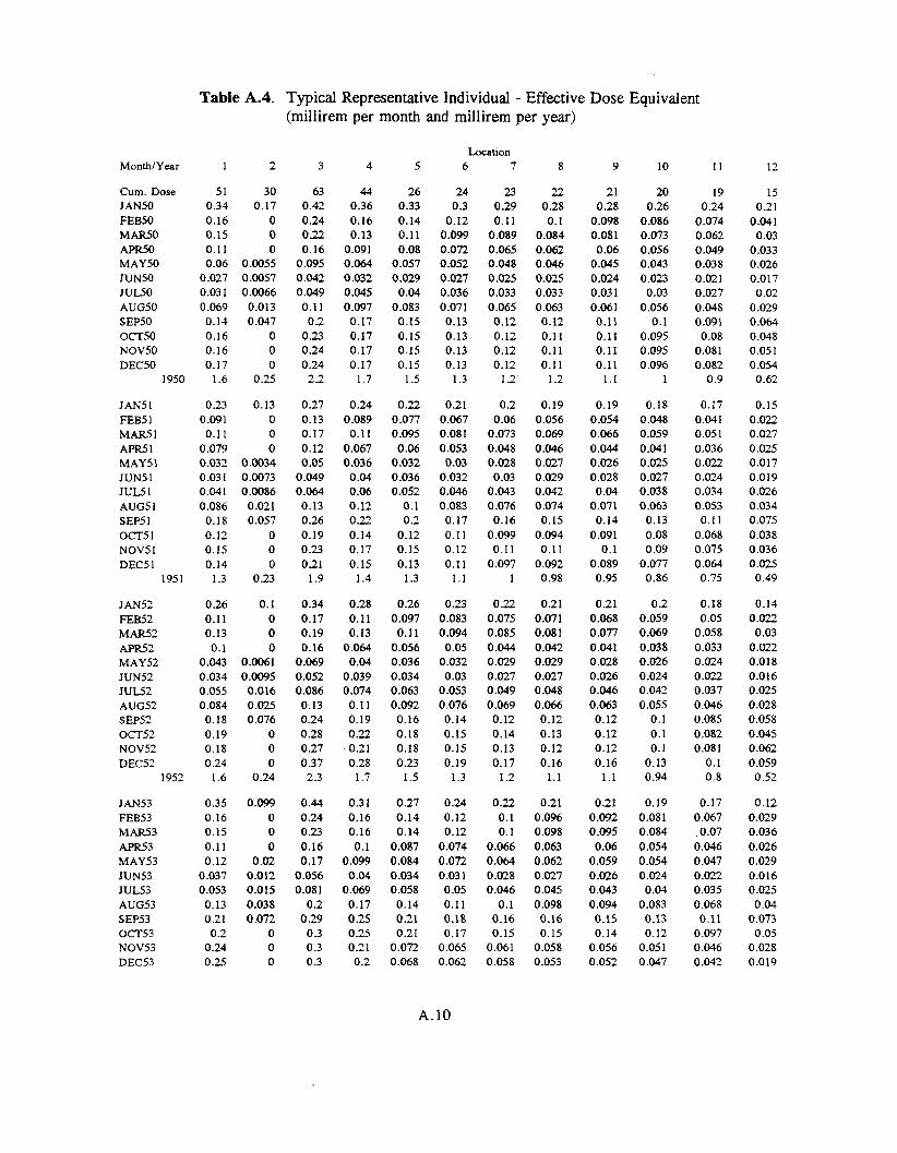
Table A.4. Typical Representative Individual - Effective Dose Equivalent
Month/Yenr
Cum. Dose JAN50 FEB5O MAR50 APR50 MAY50 JUN5O JULSO AUG5O SEP5O Om50 NOV50 DEC5O
1950
JAN51 FEB5 1 MAR51 APR5I MAY51 JUN5 1 JUL5I AUG5I SEPS 1 O m 5 1 NOV5 1 DEC5 1
1951
JAN52 FEB52 MAR52 APR52 MAY52 JUN52 JUL52 AUG52 SEP52 Om52 NOV52 DEC52
1952
JAN53 FEB53 MAR53 APRs3 MAY53 JUN53 JUL53 AUG53 SEP53 Om53 NOV53 DEC53
1
51 0.34 0.16 0.15 0.1 1 0.06
0.027 0.03 1 0.069 0.14 0.16 0.16 0.17
1.6
0.23 0.091 0.1 1
0.079 0.032 0.031 0.041 0 .086 0.18 0.12 0.15 0.14
1.3
0.26 0.11 0.13 0.1
0.043 0.034 0.055 0.084 0.18 0.19 0.18 0.24
1.6
0.35 0.16 0.15 0.11 0.12
0.037 0.053 0.13 0.21 0.2
0.24 0.25
2
30 0.17
0 0 0
0.0055 0.0057 0.0066 0.013 0.047
0 0 0
0.25
0.13 0 0 0
0.0034 0.0073 0.0086 0.021 0.057
0 0 0
0.23
0.1 0 0 0
0.0061 0.0095 0.016 0.025 0.076
0 0 0
0.24
0.099 0 0 0
0.02 0.012 0.015 0.038 0 .on
0 0 0
(millirem per month and millirem per year)
3
63 0.42 0.24 0.22 0.16
0.095 0.042 0.049 0.11 0.2
0.23 0.24 0.24 2.2
0.27 0.13 0.17 0.12 0.05
0.049 0.064 0.13 0.26 0.19 0.23 0.21
1.9
0.34 0.17 0.19 0.16
0.069 0.052 0.086 0.13 0.24 0.28 0.27 0.37 2.3
0.44 0.24 0.23 0.16 0.17
0.056 0.081
0.2 0.29 0.3 0.3 0.3
4
44 0.36 0.16 0.13
0.091 0.064 0.032 0.045 0.097 0.17 0.17 0.17 0.17
1.7
0.24 0.089 0.1 1
0.067 0.036 0.04 0.06 0.12 0 .22 0.14 0.17 0.15
1.4
0.28 0.11 0.13
0.064 0.04
0.039 0.074 0.11 0.19 0.22 0.21 0.28
1.7
0.31 0.16 0.16 0.1
0.099 0.04
0.069 0.17 0.25 0.25 0.21 0.2
5
26 0.33 0.14 0.11 0.08
0.057 0.029 0.04
0.083 0.15 0.15 0.15 0.15
1.5
0.22 0.077 0.095 0.06
0.032 0.036 0.052
0.1 0.2
0.12 0.15 0.13
1.3
0.26 0.097 0.11
0.056 0.036 0.034 0.063 0.092 0.16 0.18 0.18 0.23
1.5
0.27 0.14 0.14
0.087 0.084 0.034 0.058 0.14 0.21 0.21 0.072 0.068
1 6
24 0.3
0.12 0.099 0.072 0.052 0.027 0.036 0.071 0.13 0.13 0.13 0.13
1.3
0.21 0.067 0.081 0.053 0.03
0.032 0.046 0.083 0.17 0.11 0.12 0.1 1
1.1
0.23 0.083 0.094 0.05
0.032 0.03
0.053 0.076 0.14 0.15 0.15 0.19
1.3
0.24 0.12 0.12
0.074 0.072 0.031 0.05 0.1 1 0.18 0.17
0.065 0.062
acation 7
23 0.29 0.11
0.089 0.065 0.048 0.025 0.033 0.065 0.12 0.12 0.12 0.12
1.2
0.2 0.06
0.073 0.048 0.028 0.03
0.043 0.076 0.16
0.099 0.11
0.097 1
0.22 0.075 0.085 0.044 0.029 0.027 0.049 0.069 0.12 0.14 0.13 0.17
1.2
0.22 0.1 0.1
0.066 0.064 0.028 0.046
0.1 0.16 0.15
0.061 0.058
8
22 0.28 0.1
0.084 0.062 0.046 0.025 0.033 0.063 0.12 0.1 1 0.11 0.11
1.2
0.19 0.056 0.069 0.046 0.027 0.029 0.042 0.074 0.15
0.094 0.11 0.092 0.98
0.21 0.071 0.081 0.042 0.029 0.027 0.048 0.066 0.12 0.13 0.12 0.16
1.1
0.21 0.096 0.098 0.063 0.062 0.027 0.045 0.098 0.16 0.15
0.058 0.053
9 10
21 20 0.28 0.26
0.098 0.086 0.081 0.073 0.06 0.056
0.045 0.043 0.024 0.023 0.031 0.03 0.061 0.056 0.11 0.1 0.11 0.095 0.11 0.095 0.11 0.096
1.1 1
0.19 0.18 0.054 0.048 0.066 0.059 0.044 0.041 0.026 0.025 0.028 0.027 0.04 0.038
0.071 0.063 0.14 0.13
0.091 0.08 0.1 0.09
0.089 0.077 0.95 0.86
0.21 0.2 0.068 0.059 0.077 0.069 0.041 0.038 0.028 0.026 0.026 0.024 0.046 0.042 0.063 0.055 0.12 0.1 0.12 0.1 0.12 0.1 0.16 0.13
1.1 0.94
0.21 0.19 0.092 0.081 0.095 0.084 0.06 0.054
0.059 0.054 0.026 0.024 0.043 0.04 0.094 0.083 0.15 0.13 0.14 0.12
0.056 0.051 0.052 0.047
11
19 0.24
0.074 0.062 0.049 0.038 0.021 0.027 0.048 0.091 0.08
0.081 0 .os2 0.9
0.17 0.041 0.051 0.036 0.022 0.024 0.034 0.053 0.11
0.068 0.075 0,064 0.75
0.18 0.05
0.058 0.033 0.024 0.022 0.037 0.046 0.085 0 .OS2 0.081
0.1 0.8
0.17 0.067 0.07
0.046 0.047 0.022 0.035 0.068 0.11
0.097 0.046 0.042
12
15 0.21
0.041 0.03
0.033 0.026 0.017 0.02
0.029 0.064 0.048 0.051 0.054 0.62
0.15 0.022 0.027 0.025 0.017 0.019 0.026 0.034 0.075 0.038 0.036 0.025 0.49
0.14 0.022 0.03
0.022 0.018 0.016 0.025 0.028 0.058 0.045 0.062 0.059 0.52
0.12 0.029 0.036 0.026 0.029 0.016 0.025 0.04
0.073 0.05
0.028 0.019
A. 10

Table A.4. (contd)
1 6
1.3
0.33 0.08
0.082 0.075 0.056 0.048 0.049 0.067 0.11
0.088 0.083 0.083
1 . I
m t i o n 7 MonthJYear
1953
J AN54 FEB54 MAR54 APF54 MAY54 JUN54 JUL54 AUG54 SEP54 Om54 NOV54 DEC54
1954
1 3 4 5
1.5
0.34 0.087 0.089 0.082 0.061 0.052 0.054 0.075 0.11
0.096 0.089 0.089
1.2
8
1 . I
0.32 0.069 0.07 1 0.066 0.052 0.044 0.045 0.062 0.099 0.08
0.076 0.075
1.1
9
1.1
10
0.95
11
0.82
12
0.49
i
0.26
0.26 0 0 0
0.013 0.017 0.019 0.034 0.074
0 0 0
0.41
2
0.5 0.24 0.23 0.25
0.098 0.056 0.057 0.1 1 0.2
0.22 0.19 0.21 2.4
2.8
0.57 0.31 0.3
0.32 0.15
0.087 0.087 0.16 0.26 0.3
0.26 0.28 3.1
2
0.47 0.18 0.19 0.15
0.089 0.072 0.079 0.14 0.21 0.22 0.19 0.2 2.2
1.2
0.33 0.075 0.076 0.069 0.053 0.044 0.045 0.063
0.1 0.084 0.08 0.08
1.1
0.32 0.068 0.07 0.064 0.05
0.042 0.043 0.06
0.098 0.078 0.074 0.014
1
0.31 0.063 0.064 0.06
0.049 0.04
0.041 0.057 0.093 0.073 0.07
0.069 0.99
0.31 0.058 0.059 0.055 0.044 0.037 0.038 0.052 0.087 0.067 0.065 0 .OM 0.93
0.28 0.03 1 0.039 0.037 0.035 0.03
0.03 1 0.039 0.072 0.05
0.047 0.043 0.73
JAN55 FEB55 MAR55 APR55 MAY55 JUN55 JUL55 AUG.55 SEP55 Om55 NOV55 DEC55
1955
JAN56 FEB56 MAR56 APR56 MAY56 JUN56 JUL56 AUG56 SEP56 Om56 NOV56 DEC56
1956
0.54 0.15 0.23 0.22 0.28
0.087 0.066 0.15 0.25 0.28 0.27 0.35 2.9
0.65 0.27 0.3
0.13 0 .on 0.064 0.1 1 0.23 0.34 0.22 0.27 0.39 3.1
0.31 0 0 0
0.025 0.022 0.025 0.043 0.092
0 0 0
0.52
0.38 0 0 0
0.013 0.028 0.046 0.083 0.13
0 0 0
0.67
0.61 0.2
0.32 0.3
0.38 0.13 0.1
0.21 0.3 1 0.36 0.35 0.43
3.7
0.73 0.36 0.38 0.19 0.11
0.095 0.16 0.31 0.42 0.29 0.35 0.46 3.9
0.52 0.15 0.24 0.18 0.18
0.097 0.091 0.18 0.24 0.26 0.25 0.26 2.6
0.59 0.24 0.21 0.11
0.075 0.076 0.14 0.24 0.31 0.2
0.23 0.29 2.7
0.39 0.073 0.11
0.093 0.1
0.07 0.057 0.083 0.11 0.12 0.12 0.13
1.5
0.47 0.12 0.12
0.079 0.057 0.054 0.082 0.11 0.15
0.099 0.1
0.11 1.6
0.38 0.068 0.098 0.086 0.093 0.065 0 .05 1 0.075 0.11 0.11 0.11 0.12
1.4
0.46 0.11 0.11
0.073 0 .OS3 0.05
0.074 0.1
0.14 0.093 0.094
0.1 I .5
0.38 0.066 0.093 0.081 0 .086 0.061 0.048 0.07 0.1 0.1
0.11 0.11
1.3
0.46 0.1 0.1
0.067 0.049 0.046 0.069 0.098 0.14 0.09
0.089 0.095
1.4
0.38 0.062 0.089 0.078 0.083 0.06
0.047 0.068
0.1 0.097
0.1 0.1 1.3
0.45 0.095 0.097 0.065 0.048 0.045 0.068 0.094 0.13
0.085 0.084 0.09
1.4
0.38 0.061 0.087 0.076 0 .os 1 0.058 0.045 0.066
0.1 0.096
0.1 0.1 1.2
0.45 0.094 0.095 0.064 0.046 0.044 0.066 0.092 0.13
0.084 0.083 0.088
1.3
0.37 0.058 0.082 0.072 0.077 0.056 0.043 0.062 0.095 0.089 0.096 0.093
1.2
0.44 0.087 0.089 0.061 0.044 0.042 0.062 0.087 0.12 0.08
0.077 0.081
1.3
0.36 0.054 0.074 0.067 0.07
0.052 0.04
0.056 0.089 0.08 1 0.089 0.086
1.1
0.43 0.081 0.083 0.057 0.041 0.038 0.057 0.079 0.12
0.075 0.071 0.072
1.2
0.34 0.038 0.047 0.042 0.05
0.042 0.031 0.041 0.075 0.055 0.054 0.04 0.86
0.4 0.052 0.052 0.044 0.034 0.03 1 0.045 0.061 0.097 0.06
0.049 0.043 0.97
JAN57 FEB57 MAR57 APR57 MAY57 JUN57 JUL57 AUGS7 SEP57 Om57 NOV57 DEC57
0.65 0.35 0.42 0.35 0.11 0.08 0.19 0.33 0.49 0.33 0.37 0.52
0.32 0 0 0
0.023 0.038 0.088 0.12 0.19
0 0 0
0.73 0.44 0.5
0.44 0.16 0.12 0.25 0.42 0.57 0.42 0.46 0.62
0.61 0.28 0.22 0.2
0.097 0.089
0.2 0.32 0.38 0.28 0.3 1 0.39
0.42 0.1 1
0.094 0.1 1
0.069 0.054 0 .095 0.13 0.17 0.14 0.14 0.16
0.41 0.1
0.084 0.095 0.064 0.048 0.085 0.11 0.16 0.13 0.14 0.15
0.4 0.094 0.076 0.085 0.059 0.044 0 .os 0.1 1 0.15 0.12 0.13 0.14
0.4 0.089 0.067 0.077 0.057 0.042 0.075 0.099 0.14 0.11 0.12 0.13
0.39 0.086 0.061 0.072 0.054 0.039 0.07
0.091 0.13 0.11 0.11 0.12
0.39 0.079 0.056 0.066 0.051 0.037 0.065 0.085 0.12 0.1
0.1 1 0.12
0.38 0.071 0.051 0.062 0.047 0.034 0.06
0.078 0.12
0.098 0.11 0.1 1
0.35 0.043 0.028 0.043 0.038 0.026 0.048 0.062
0.1 0.081 0.083 0.069
A . l l

Month/Year
1957
JAN58 FEB58 MAR58 AP-8 MAY58 JUN58 JUL58 AUG58 SEP58 Om58 NOV58 DEC58
1958
JAN59 FEB59 MAR59 APR59 MAY59 JUN59 JUL59 AUG59 SEP59 Om59 NOV59 DEC59
1959
JAN60 FEB60 MAR60 APR60 MAY60 JUN60 JUL60 AUG60 SEP60 OCI-60 NOV60 DEC60
1960
JAN61 FEB6 1 MAR61 APR6 1 MAY61 JUN6 1 JUL6 1 AUG61 SEP6 1 OCI-6 1 NOV61 DEC6 1
1
4 2
0.79 0.39 0.29 0.29 0.15 0.094 0.19 0.33 0.41 0 3 9 0.4
0.43 4.2
0.63 0.28 0.24 0.19 0.1 I
0.078 0.093 0.24 0.28 0.16 0 2 1 0 2 9 2.8
0.99 0 3 2 0.43 02
0.19 0.13 0.13 0.29 0.48 0 3 2 0.45 0.49 4.4
1.1 0 3 035 0.29 0.16 0.08 0.13 023 0.29 023 0.23 0 2 4
2
0.78
032 0 0 0
0.036 0.06
0.098 0.13 0 3
0 0 0
0.85
0.38 0 0 0
0.041 0.058 0.063 0.17 0.18
0 0 0
0.89
0.5 0 0 0
0.075 0.081 0.079 0.19 03
0 0 0
1 2
0.45 0 0 0
0-063 0.058 0.11 0.13 0.12
0 0 0
3
5.1
0.86 0.48 0.37 0.39 0.21 0.13 0.26 0.41 0.44 0.49 0.47 0.51
5
0.67 0.36 0.32 0.25 0.16 0.11 0.13 0.28 0.34 011 0.28 0.36 3.5
1.1 0.39 0.5 028 0.26 0.18 0.19 0.34 0.51 0.38 0.51 0.59 5.3
1.2 0.39 0.45 0.4
0.21 0.12 0.16 0.28 0.34 0.28 0.28 0.27
4
3.4
0.65 0.26 0.23 0.21 0.12 0.1 0.2 0.3
0.29 0.33 0.28 0.29 3.3
0.55 0.23 0.21 0.15 0.1 1
0.083 0.12 0.21 0.26 0.15 0.2
0.26 2.5
0.93 0.25 0.27 0.19 0.17 0.14 0.17 0.25 0.34 0.26 0.33 0.38 3.7
0.91 0.25 0.3
0.27 0.15
0.098 0.13 0.22 0.24 0.19 0.19 0.16
Table A.4. (contd)
5
1.7
0.42 0.12 0.1
0.12 0.08
0.056 0.088 0.11 0.11 0.14 0.12 0.12
1.6
0.44 0.1
0.11 0.086 0.066 0.049 0.06
0.069 0.14
0.075 0.11 0.14
1.4
0.73 0.13 0.13 0.11
0.095 0.078 0.088 0.083 0.14 0.12 0.13 0.17
2
0.64 0.15 0.18 0.19
0.096 0.064 0.049
0.1 0.14
0.097 0.11
0.084
I 6
1.6
0.41 0.11
0.093 0.1 1
0.074 0.049 0.078
0.1 0.1
0.13 0.12 0.1 1
1.5
0.43 0.093 0.098 0.079 0.059 0.044 0.053 0.062 0.13
0.069 0.11 0.13
1.4
0.71 0.12 0.12 0.1
0.087 0.069 0.079 0.075 0.13 0.11 0.12 0.16
1.9
0.63 0.14 0.17 0.18
0.091 0.058 0.044 0.096 0.14
0.094 0.1
0.082
A. 12
m t i o n 7
1.5
0.4 0.1
0.085 0.1
0.068 0.044 0.073 0.096
0.1 0.12 0.11 0.11
1.4
0.43 0.087 0.092 0.074 0.055 0.039 0.049 0.059 0.13
0.066 0.1
0.13 1.3
0.7 0.12 0.11
0.093 0.082 0.064 0.074 0.071 0.13 0.11 0.12 0.15
1.8
0.62 0.14 0.16 0.17
0.087 0.053 0.042 0.093 0.13 0.092 0.098 0.079
8
1.4
0.39 0.089 0.076 0.094 0.064 0.042 0.067 0.087 0.093 0.1 1
0.099 0.096
1.3
0.42 0.078 0.085 0.07
0.052 0.038 0.046 0.054 0.12
0.062 0.095 0.12
1.2
0.69 0.11 0.1
0.087 0.078 0.062 0.071 0.065 0.12
0.098 0.11 0.14
1.7
0.6 0.13 0.15 0.16
0.085 0.052 0.039 0.087 0.13
0.085 0.089 0.073
9 10
1.3 1.3
0.38 0.38 0.085 0.079 0.071 0.065 0.089 0.084 0.061 0.058 0.039 0.037 0.062 0.058 0.08 0.075
0.088 0.085 0.1 0.093
0.094 0.089 0.089 0.083
1.2 1.2
0.42 0.42 0.073 0.067 0.08 0.075
0.066 0.063 0.049 0.047 0.036 0.033 0.043 0.041 0.051 0.048 0.11 0.11
0.059 0.056 0.09 0.085 0.11 0.11
1.2 1.1
0.68 0.67 0.11 0.11
0.095 0.09 0.083 0.079 0.074 0.071 0.058 0.055 0.067 0.063 0.061 0.057 0.12 0.11
0.094 0.09 0.1 0.096
0.13 0.12 1.7 1.6
0.59 0.58 0.12 0.12 0.14 0.14 0.16 0.15
0.083 0.081 0.049 0.047 0.037 0.036 0.083 0.08 0.12 0.12
0.083 0.08 0.086 0.082 0.071 0.069
11
1.2
0.37 0.074 0.06
0.079 0.054 0.033 0.053 0.07
0.082 0.087 0.085 0.077
1.1
0.41 0.062 0.07
0.062 0.043 0.03
0.038 0.045 0.11
0.053 0.081
0.1 1.1
0.66 0.1 1
0.085 0.074 0.067 0.051 0.059 0.053 0.1 1
0.086 0.091 0.12
1.5
0.57 0.11 0.13 0.15 0.08
0.044 0.034 0.076 0.12
0.079 0.078 0.069
12
0.98
0.34 0.041 0.041 0.058 0.045 0.026 0.041 0.055 0.073 0.065 0.058 0.052
0.9
0.4 0.038 0.052 0.046 0.035 0.025 0.03 1 0.036 0.094 0.044 0.063 0.08 0.94
0.6 0.076 0.054 0.054 0.053 0.042 0.05
0.043 0.09 0.072 0.06
0.074 1.3
0.52 0.071 0.079 0.12
0.073 0.038 0.03
0.062 0.1 1
0.073 0.056 0.045

MonthlYear
1961
JAN62 FEB62 MAR62 OR62 MAY62 JUN62 JUL62 AUG62 SEP62 Om62 NOV62 DEC62
1962
JAN63 FEB63 MAR63 APR63 MAY63 JUN63 JUL63 AUG63 SEP63 Om63 NOV63 DEC63
I963
JAN64 FEB64 MAR64 APR64 MAY64 JUN64 JUL64 AUG64 SEP64 Om64 NOV64 DEC64
1964
IAN65 FEB65 MAR65 APR65 MAY65 JUN65 JUL65 AUG65 SEP65 Om65 NOV65 DEC65
1
3.6
0.86 0.23 0.37 0.34 0.19 0.14 0.16 0.28 0.52 0.24 0.2
0.21 3.7
0.66 0.16 0.23 0.2
0.13 0.087 0.11 0.19 0.3 1 0.23 0.22 0.24 2.8
0.6 0.2
0.26 0.3
0.22 0.087 0.088 0.18 0.31 0.13 0.22 0.22 2.8
0.41 0.13 0.16 0.14
0.085 0.073 0.077 0.12 0.22 0.18 0.15 0.14
2
0.94
0.57 0 0 0
0.066 0.1 0.1
0.16 0.26
0 0 0
1.3
0.52 0 0 0
0.045 0.067 0.084 0.13 0.53 0.44 0.4
0.45 4.7
0.82 0.39 0.49 0.57 0.43 0.17 0.17 0.32 0.54 0.26 0.42 0.42
5
0.59 0.26 0.32 0.28 0.17 0.14 0.15 0.22 0.37 0.33 0.28 0.27
3
4.4
0.92 0.28 0.43 0.45 0.27 0.2
0.23 0.36 0.59 0.31 0.26 0.28 4.6
0.7 0.2
0.27 0.25 0.17 0.12 0.15 0.22 0.31 0.27 0.24 0.26 3.2
0.61 0.25 0.3
0.36 0.29 0.12 0.12 0.21 0.31 0.17 0.25 0.24 3.2
0.44 0.16 0.2
0.18 0.12 0.1 0.1
0.15 0.22 0.19 0.17 0.16
Table A.4. (contd)
Location 4 5 6 7 8
3.1 1.9 1.8 1.8 1.7
0.79 0.68 0.18 0.11 0.25 0.13 0.23 0.15 0.17 0.11 0.15 0.084 0.19 0.11 0.28 0.15 0.43 0.26 0.2 0.13
0.17 0.1 0.19 0.12 3.2 2.1
0.65 0.12 0.16 0.16 0.09
0.083 0.12 0.16 0.2
0.18 0.14 0.15 2.2
0.49 0.16 0.18 0.16 0.15
0.082 0.095 0.15 0.2
0.12 0.16 0.13 2.1
0.34 0.081 0.11
0.095 0.074 0.068 0.077
0.1 0.14 0.11 0.1 1 0.1
0.59 0.068 0.066 0.081 0.05
0.041 0.044 0.049 0.075 0.06 0.06
0.058 1.2
0.38 0.07
0.077 0.083 0.083 0.048 0.039 0.052 0.09
0.048 0.062 0.055
1.1
0.28 0.046 0.06
0.057 0.045
0.033 0.036 0.064 0.036 0.037 0.041
0.038
0.68 0.1
0.13 0.15
0.097 0.075 0.11 0.14 0.25 0.13
0.098 0.1 1 2.1
0.58 0.065 0.061 0.075 0.046 0.035 0.038 0.043 0.07 1 0.054 0.056 0.054
1.2
0.37 0.065 0.072 0.076 0.075 0.043 0.033 0.046 0.086 0.044 0.056 0.051
1
0.27 0.043 0.056 0.053 0.04
0.033 0.029 0.03 1 0.061 0.033 0.034 0.038
A. 13
0.67 0.099 0.12 0.14 0.092 0.07 0.1
0.13 0.24 0.13
0.095 0.11
2
0.58 0.06
0.057 0.07
0.043 0.032 0.034 0.041 0.068 0.051 0.053 0.051
1.1
0.37 0.061 0.068 0.071 0.07
0.038 0.029 0.044 0.083 0.042 0.053 0.047 0.98
0.27 0.039 0.052 0 .049 0.036 0.03
0.026 0.029 0.059 0.03 1 0.032 0.036
0.66 0.092 0.11 0.13
0.088 0.068 0.097 0.13 0.23 0.13
0.087 0.1 1.9
0.58 0.055 0.051 0.065 0.041 0.03
0.032 0.037 0.064 0.045 0.047 0.045
1.1
0.36 0.056 0.062 0.066 0.066 0.036 0.027 0.04
0.079 0.039 0.048 0.042 0.93
0.26 0.036 0.049 0.046 0.035 0.029 0.025 0.027 0.056 0.027 0.029 0.033
9 10
1.6 1.6
0.66 0.65
0.1 0.099 0.12 0.12
0.084 0.081 0.065 0.062 0.094 0.091 0.12 0.12 0.22 0.21 0.13 0.13
0.084 0.081 0.098 0.094
1.9 1.8
0.57 0.57 0.053 0.05 0.048 0.045 0.062 0.058 0.039 0.037 0.028 0.026 0.029 0.027 0.034 0.031 0.061 0.058 0.041 0.038 0.044 0.042 0.042 0.039
1.1 1
0.36 0.36 0.052 0.048 0.058 0.055 0.062 0.059 0.062 0.058 0.034 0.031 0.025 0.023 0.037 0.035 0.016 0.073 0.036 0.035 0.044 0.04 0.04 0.037 0.89 0.85
0.26 0.26 0.034 0.033 0.046 0.044 0.044 0.042 0.033 0.031 0.026 0.025 0.023 0.021 0.025 0.023 0.054 0.052 0.025 0.023 0.026 0.024 0.031 0.029
0.09 0.088
11
1.5
0.65 0.086 0.095 0.12
0.077 0.058 0.087 0.11 0.21 0.13
0.078 0.09
1.8
0.57 0.049 0.042 0.054 0.035 0.023 0.024 0.029 0.056 0.035 0.04
0.037 0.99
0.35 0.045 0.051 0.055 0.054 0.028 0.02
0.032 0.07
0.033 0.036 0.035 0.81
0.25 0.03
0.041 0.04
0.029 0.023 0.019 0.021 0.05
0.021 0.022 0.027
12
1.3
0.62 0.07
0.064 0.092 0.063 0.05
0.078 0.1
0.18 0.1 1
0.056 0.064
1.5
0.56 0.035 0.03
0.036 0.027 0.018 0.018 0.022 0.05
0.03 1 0,041 0.026 0.89
0.34 0.03 1 0.034 0.042 0.042 0.022 0.015 0.025 0.067 0.029 0.025 0.019 0.69
0.24 0.022 0.032 0.034 0.023 0.018 0.015 0.016 0.045 0.017 0.016 0.02

MonthlYear
1965
JAN66 FEB66 MAR66 APR66 MAY66 JUN66 JUM6 AUG66 SEP66 Om66 NOV66 DEC66
1966
JAN67 FEB67 MAR67 APR67 MAY67 JUN67 JUM7 AUG67 SEP67 Om67 NOV67 DEC67
1967
JAN68 FEB68 MAR68 APR68 MAY68 JUN68 JUM8 AUG68 SEP68 Om68 NOV68 DEC68
1968
J AN69 FEB69 MAR69 APR69 MAY69 JUN69 JUM9 AUG69 SEP69 OCr69 NOV69 DEC69
1
1.9
0.29 0.094 0.12 0.12
0.083 0.054 0.019 0.045 0.23 0.12 0.1
0.12 1.4
0.3 1 0.11 0.11 0.14 0.13
0.048 0.061 0.12 0.2
0.1 1 0.099 0.097
1.5
0.25 0.12
0.098 0.097 0.097 0.041 0.039 0.099 0.14
0.086 0.077 0.071
1.2
0.17 0.049 0.077 0.046 0.034 0.044 0.044 0.085 0.1 1
0.04 1 0.033
2
3.4
0.39 0.18 0.23 0.23 0.16 0.1
0.036 0.08 0.39 0.23 0.19 0.23 2.4
0.42 0.21 0.22 0.27 0.26
0.094 0.12 0.22 0.35 0.21 0.19 0.19 2.7
0.33 0 2 3 0.19 0.19 0.18
0.078 0.075 0.18 0.23 0.16 0.15 0.14 2.1
0 .z 0.095 0.15 0.092 0.066 0.084 0.083 0.16 0.18
0.077 0.062
3
2.2
0.3 0.11 0.14 0.14 0.11
0.073 0.025 0.046 0.22 0.14 0.12 0.14
1.6
0.33 0.13 0.15 0.17 0.16
0.069 0.084 0.14 0.21 0.13 0.12 0.12
1.8
0.26 0.13 0.12 0.12 0.12
0.056 0.053 0.12 0.15 0.1
0.091 0.088
1.4
0.18 0.066 0.097 0.065 0.046 0.058 0.056 0.095 0.1 1
0.047 0.039
4
1.4
0.24 0.071 0.086 0.071- 0.074 0.058 0.021 0.032 0.15
0.096 0.079 0.089
1.1
0.27 0.081
0.1 0.1 1
0.085 0.051 0.071 0.1 1 0.16
0.087 0.077 0.079
1.3
0.22 0.07
0.079 0.078 0.07 0.04 0.044 0.084 0.1 1
0.065 0.056 0.057 0.97
0.15 0.046 0.058 0.041 0.029 0.042 0.043 0.069 0.081 0.033 0.027
Table A.4. (contd)
5
0.77
0.2 0.03
0.038 0.037 0.037 0.024
0.0076 0.007 0.066 0.053 0.042 0.045 0.59
0.23 0.047 0.057 0.062 0.046 0.033 0.035 0.039 0.075 0.04
0.036 0.038 0.74
0.18 0.033 0.039 0.039 0.037 0.02
0.018 0.03
0.054 0.025 0.026 0.025 0.53
0.13 0.023 0.031 0.025 0.016 0.018 0.016 0.024 0.045 0.015 0.013
1 6
0.72
0.2 0.028 0.035 0.034 0.033 0.02
0.0064 0.0062 0.063 0.051 0.041 0.042 0.56
0.23 0.045 0.055 0.059 0.043 0.029 0.03
0.035 0.072 0.038 0.034 0.036
0.7
0.18 0.03 1 0.036 0.027 0.027 0.013 0.01 1 0.019 0.046 0.016 0.018 0.017 0.44
0.12 0.017 0.022 0.018 0.01 1 0.01
0.0098 0.016 0.041 0.012 0.01 1
m t i o n 7
0.69
0.2 0.027 0.033 0.032 0.03 1 0.018
0.0059 0.0059 0.061 0.05
0.041 0.04 0.54
0.22 0.043 0.052 0.057 0.04
0.026 0.028 0.033 0.07
0.036 0.032 0.035 0.68
0.17 0.029 0.034 0.025 0.024 0.01 1
0.0093 0.016 0.044 0.014 0.016 0.015 0.41
0.12 0.015 0.018 0.015
0.0092 0.0082 0.0081 0.014 0.041 0.01 1 0.01 1
8
0.65
0.19 0.025 0.03 0.03
0.029 0.017
0.0055 0.0054 0.058 0.046 0.038 0.037 0.52
0.22 0.04
0.049 0.054 0.03 9 0.025 0.027 0.03 1 0.066 0.034 0.03
0.032 0.65
0.17 0.027 0.031 0.024 0.023 0.01 1
0.0088 0.015 0.043 0.013 0.015 0.014
0.4
0.12 0.014 0.017 0.014
0.0088 0.0077 0.0077 0.013 0.04 0.01
0.0099
9 10
0.63 0.6
0.19 0.19 0.023 0.022 0.029 0.027 0.029 0.027 0.027 0.026 0.016 0.015
0.0052 0.0048 0.005 0.0046 0.056 0.054 0.044 0.042 0.038 0.037 0.036 0.034
0.5 0.48
0.22 0.22 0.039 0.038 0.047 0.046 0.052 0.051 0.037 0.036 0.024 0.022 0.025 0.023 0.029 0.027 0.064 0.062 0.032 0.031 0.028 0.027 0.03 0.028 0.63 0.61
0.17 0.17 0.025 0.024 0.03 0.028 0.023 0.023 0.022 0.022 0.01 0.01
0.0085 0.0082 0.014 0.014 0.043 0.043 0.013 0.013 0.014 0.014 0.014 0.014 0.39 0.38
0.12 0.12 0.014 0.013 0.017 0.016 0.014 0.014
0.0085 0.0082 0.0074 0.0071 0.0074 0.0072 0.013 0.012 0.04 0.04 0.01 0.0098
0.0098 0.0096
1 1
0.58
0.19 0.021 0.025 0.025 0.024 0.013
0.0045 0.0043 0.052 0.04
0.036 0.033 0.47
0.21 0.036 0.044 0.048 0.034 0.02
0.02 1 0.026 0.059 0.029 0.025 0.026 0.58
0.17 0.022 0.026 0.022 0.02 1
0.0097 0.0079 0.013 0.042 0.012 0.013 0.013 0.37
0.12 0.013 0.016 0.013
0.0078 0 .M67 0.0069 0.012 0.04
0.0096 0.0094
12
0.5
0.18 0.016 0.016 0.019 0.02
0.01 1 0.0039 0.0034 0.046 0.037 0.027 0.021
0.4
0.2 0.026 0.034 0.039 0.03
0.016 0.017 0.021 0.055 0.023 0.019 0.019 0.5
0.16 0.015 0.019 0.02
0.018 0.0086 0.0069 0.01 1 0.041 0.01
0.0089 0.0083
0.33
0.12 0.0099 0.013 0.01 1
0.0067 0.0056 0.006 0.01
0.039 0.0083 0.0087
0.042 0.079 0.051 0.037 0.017 0.013 0.011 0.011 0.011 0.011 0.01 0.007
A. 14

Table A.4. (contd)
Month/Year
1969
JAN70 FEB7O MAR70 APR70 MAY70 JUN7O JUL70 AUG70 SEW0 o m 0 NOV70 DEC70
1970
JAN71
1
0.77
0.13 0.002 0.01 1 0.042 0.039 0.028 0.046 0.035 0.11
0.057 0.054 0.054 0.61
0.054
2
1.3
0.19 0.0053 0.022 0.082 0.074 0.054 0.087 0.066 0.18 0.11 0.1 0.1 1.1
0.097
3
0.91
0.14 0.0048 0.014 0.053 0.047 0.037 0.059 0.043 0.11 0.07
0.067 0.067 0.72
0.06
4
0.66
0.11 0.003 1 0.0091 0.033 0.024 0.02
0.03 9 0.03 1 0.083 0.048 0.043 0.042 0.49
0.032
Location 5 6 7
0.37 0.3 0.28
0.087 0.0029 0.0044 0.016 0.014 0.011 0.016 0.013 0.049 0.024 0.022 0.021 0.28
0.081 0.0032 0.0029 0.01 1 0.01 1
0.0074 0.011 0.01
0.042 0.019 0.017 0.016 0.23
0.079 0.003 0.0022 0.0093 0.0098 0.0062 0.0091 0.0094
0.04 0.017 0.016 0.015 0.22
0.018 0.013 0.011
8
0.27
0.078 0.0029 0.002
0.0087 0.0095 0.0059 0.0086 0.009 0.039 0.016 0.015 0.014 0.21
0.01
9
0.27
0.078 0.0029 0,002
0.0084 0.0094 0.0058 0.0084 0.0089 0.039 0.016 0.015 0.014 0.21
0.01
10
0.27
0.078 0.003
0.0018 0.0081 0.0093 0.0056 0.0081 0.0088 0.038 0.016 0.015 0.013
0.2
0.0097
11 12
0.26 0.24
0.077 0.076 0.0029 0.0022 0.0017 0.0013 0.0077 0.0062 0.0093 0.0084 0.0053 0.0048 0.0078 0.0068 0.0087 0.0082 0.038 0.036 0.016 0.014 0.014 0.012 0.013 0.0089
0.2 0.18
0.0092 0.0069
A. 15

Table A S . Typical Representative Individual - Red Bone Marrow Equivalent Dose
Year
Cum. Dose
1950
1951
1952
1953
1954
1955
1956
1957
1958
1959
1960
1961
1962
1963
1964
1965
1966
1967
1968
1969
1970
1971
1
35
0.78
0.62
0.77
0.93
1.2
1.5
1.7
2.3
2.5
2.2
3.3
3
3.2
2.2
2.1
1.5
1.2
1.3
1
0.66
0.48
0.04
(millirem per year)
Location 2
26
0.29
0.25
0.25
0.27
0.46
0.58
0.73
0.81
0.88
0.93
1.3
1
1.3
3.6
3.5
2.5
2.1
2.3
1.7
1.1
0.81
0.072
3
43
1.1
0.86
1.1
1.3
1.7
2
2.2
2.9
3.1
2.7
4.1
3.9
4.1
2.5
2.4
1.7
1.4
1.6
1.2
0.8
0.57
0.047
4
33
0.87
0.7
0.87
1
1.3
1.6
1.7
2.1
2.2
2.1
3.1
2.9
3.1
1.9
1.7
1.2
1
1.2
0.88
0.61
0.42
0.028
5
26
0.83
0.66
0.8
0.88
1.1
1.3
1.4
1.7
1.7
1.6
2.3
2.4
2.5
1.4
1.2
0.89
0.76
0.91
0.65
0.45
0.32
0.022
6
25
0.8
0.62
0.75
0.82
1.1
1.3
1.4
1.6
1.7
1.6
2.3
2.3
2.5
1.4
1.2
0.87
0.74
0.9
0.61
0.41
0.3
0.017
7
25
0.77
0.6
0.73
0.79
1.1
1.3
1.4
1.6
1.6
1.5
2.2
2.3
2.4
1.4
1.2
0.84
0.73
0.88
0.58
0.39
0.28
0.015
8
24
0.75
0.59
0.7
0.75
1
1.3
1.3
1.5
1.6
1.5
2.1
2.2
2.3
1.4
1.1
0.81
0.7
0.85
0.57
0.38
0.27
0.014
9
23
0.74
0.58
0.69
0.74
1
1.3
1.3
1.5
1.5
1.5
2.1
2.2
2.3
1.3
1.1
0.8
0.69
0.84
0.56
0.38
0.27
0.014
10
23
0.72
0.56
0.66
0.71
1
1.2
1.3
1.5
1.5
1.4
2.1
2.1
2.3
1.3
1.1
0.78
0.67
0.82
0.55
0.37
0.27
0.013
11
22
0.7
0.54
0.63
0.68
1
1.2
1.3
1.4
1.5
1.4
2
2.1
2.2
1.3
1.1
0.76
0.65
0.8
0.54
0.36
0.26
0.013 0
12
19
0.61
0.46
0.55
0.51
0.86
1
1.1
1.2
1.2
1.2
1.7
1.7
2
1.2
0.91
0.68
0.56
0.69
0.47
0.33
0.24
1.0091
A. 16

Table A.6. Typical Representative Individual - Lower Large Intestine Equivalent Dose (millirem per year)
Year
Cum. Dose
1950
1951
1952
1953
1954
1955
1956
1957
1958
1959
1960
1961
1962
1963
1964
1965
I966
1967
1968
1969
1970
1971
1
299
12
9.9
13
16
17
20
21
29
28
-1 4
23
17
16
13
15
9.8
6
6.8
5.9
3.3
2.9
0.3 1
2
124
0.3 1
0.27
0.27
0.28
0.49
0.61
0.77
0.83
0.89
0.95
1.3
1
1.4
25
29
19
1 1
13
1 1
6.3
5.5
0.59
3
3 93
18
I5
19
23
23
27
27
37
35
19
29
22
20
17
19
12
7.3
8.7
7.4
4.3
3.7
0.36
4
262
13
11
14
16
15
18
18
23
22
13
19
15
13
1 1
12
7.6
4.8
6
5
3
2.4
5
125
11
9.6
12
12
6.1
6.9
7.1
7.9
7.4
5.8
7.2
5.8
6
4.3
4.4
3.2
1.9
2.5
2.1
1.3
0.96
Location 6
107
9.1
8.1
9 .I
9.6
5.3
6
6.2
6.9
6.5
5.1
6.4
5.2
5.5
3.8
3.9
2.9
1.7
2.2
1.3
0.78
0.52
7
96
8.1
7.3
8.6
8.5
4.9
5.5
5.7
6.2
5.8
4.7
5.8
4.8
5.1
3.5
3.5
2.6
1.5
2.1
1.1
0.61
0.4
8
90
7.8
6.9
8.2
8.1
4.7
5.3
5.5
5.5
5.1
4.3
5.2
4.3
4.6
3.2
3.2
2.4
1.4
1.9
0.98
0.58
0.38
9
83
7.4
6.6
7.8
7.7
4.5
5.1
5.3
5
4.5
3.9
4.7
3.9
4.3
2.9
2.8
2.1
1.3
1.7
0.92
0.55
0.36
10
74
6.4
5.8
6.5
6.6
4.1
4.6
4.8
4.4
3.9
3.5
4.3
3.6
4
2.6
2.5
1.9
1.2
1.6
0.86
0.53
0.35
1 1
63
5.2
4.7
5.1
5.3
3.5
3.9
4.1
3.8
3.4
3.1
3.8
3.3
3.7
2.3
2.3
1.7
1
1.4
0.79
0.51
0.34
12
38
2.6
2.2
2.4
2.3
2.1
2.2
2.5
2.4
2.1
2.2
2.6
2.3
2.8
1.7
1.5
1.2
0.76
1
0.61
0.43
0.29
0.18 0.067 0.029 0.021 0.019 0.018 0.017 0.015 0.011
A.17

Table A.7. Occupational Representative Individual - Effective Dose Equivalent (millirem per month and millirem per year)
Month/Year
Cum. Dose JAN50 FEB5O MAR50 APR50 MAY50 JUN5O JULSO AUGSO SEP5O OCT50 NOV50 DECSO
1950
JAN51 FEB5 1 MAR51 APR5 1 MAY5 1 JUNS 1 JUL5 1 AUG51 SEP5 1 O n 5 1 NOV5 1 DECS 1
1951
J AN52 FEB52 MAR52 MR52 MAY52 JUN52 JUL52 AUG52 SEP52 OCT52 NOV52 DEC52
1952
JAN53 FEB53 MAR53 MR53 MAY53 JUN53 JUL53 AUG53 SEP53 Om53 NOV53 DEC53
1
520 0.94 0.88 0.86 0.62 0.36 0.16 0.18 0.4
0.64 0.98 0.99 0.98
8
0.63 0.72 0.85 0.55 0.2
0.19 0.24 0.54 0.88 0.83 0.93 0.89
7.5
0.91 0.82 0.89 0.8
0.31 0.22 0.37 0.57
1.1 1.5 1.3 1.7 10
1.8 1.3 1.3
0.96 0.92 0.26 0.36 0.91
1.2 1.6 1.9 2.1
2
908 1.8 1.7 1.7 1.3
0.72 0.31 0.36 0.8 1.3 1.9
2 2
16
1.2 1.4 1.7 1.1 0.4
0.38 0.47
1.1 1.7 1.6 1.8 1.7 15
1.8 1.6 1.7 1.6
0.61 0.43 0.73
1.1 2
2.8 2.5 3.3 20
3.4 2.4 2.5 1.9 1.8
0.52 0.71
1.8 2.3 3.1 3.4 3.6
3
505 1.3 1.2 1.2
0.87 0.52 0.23 0.27 0.59 0.9 1.3 1.3 1.3 11
0.83 0.92
1 . I 0.75 0.29 0.27 0.35 0.76
1.2 1.1 1.3 1.2 10
1.3 1.1 1.2 1.1
0.45 0.32 0.53 0.79
1.4 1.9 1.7 2.3 14
2.1 1.6 1.7 1.3 1.2
0.37 0.52
1.3 1.6 2.1 1.9 1.9
4
290 0.93 0.79 0.67 0.48 0.34 0.17 0.25
. 0.51 0.74 0.95 0.94 0.9 7.7
0.61 0.59 0.71 0.41 0.2 0.22 0.32 0.66
1 0.84 0.91 0.81 7.3
0.94 0.68 0.77 0.42 0.25 0.23 0.44 0.66
1 1.4 1.3 1.7 9.8
1.2 1
1.1 0.76 0.68 0.26 0.43
1.1 1.3 1.7 1.2 1.1
5
101 0.74 0.65 0.55 0.4
0.29 0.15 0.2
0.41 0.59 0.76 0.76 0.74
6.2
0.47 0.45 0.54 0.33 0.17 0.19 0.26 0.51 0.8
0.66 0.73 0.64 5.7
0.75 0.52 0.6
0.33 0.2
0.18 0.34 0.5
0.74 1
0.97 1.2 7.4
0.94 0.78 0.84 0.56 0.52 0.21 0.33 0.79
1 1.2
0.32 0.3
6
87 0.59 0.54 0.45 0.33 0.25 0.13 0.17 0.33 0.47 0.61 0.6
0.61 5.1
0.36 0.35 0.42 0.27 0.15 0.16 0.22 0.4
0.63 0.52 0.58 0.5 4.6
0.58 0.4 0.46 0.26 0.17 0.15 0.27 0.37 0.54 0.77 0.73 0.94 5.7
0.7 0.59 0.63 0.42 0.4
0.17 0.26 0.59 0.74 0.91 0.28 0.27
Location 7
79 0.52 0.48 0.4
0.29 0.22 0.12 0.16 0.3
0.42 0.54 0.54 0.54 4.5
0.32 0.3
0.36 0.23 0.13 0.14 0.2
0.35 0.56 0.46 0.51 0.44
4
0.52 0.35 0.4 0.22 0.15 0.13 0.24 0.32 0.46 0.65 0.62 0.81 4.9
0.59 0.51 0.53 0.35 0.33 0.15 0.23 0.51 0.64 0.78 0.27 0.25
8
74 0.49 0.45 0.38 0.28 0.21 0.12 0.15 0.29 0.4
0.52 0.51 0.51 4.3
0.29 0.28 0.34 0.22 0.13 0.14 0.2
0.34 0.54 0.44 0.48 0.42 3.8
0.49 0.33 0.38 0.21 0.15 0.13 0.23 0.3 1 0.43 0.62 0.59 0.76 4.6
0.53 0.47 0.5
0.33 0.32 0.15 0.23 0.49 0.61 0.74 0.25 0.23
9
70 0.47 0.43 0.36 0.27 0.2
0.1 1 0.15 0.27 0.38 0.49 0.49 0.49 4.1
0.28 0.26 0.32 0.21 0.12 0.13 0.18 0.32 0.51 0.42 0.46 0.4 3.6
0.47 0.31 0.36 0.2
0.14 0.12 0.22 0.29 0.41 0.59 0.56 0.72 4.4
0.5 0.44 0.47 0.31 0.3
0.14 0.21 0.46 0.58 0.7
0.25 0.23
10
64 0.38 0.37 0.32 0.25 0.19 0.1 1 0.14 0.25 0.33 0.42 0.42 0.42 3.6
0.24 0 23 0.28 0.19 0.11 0.12 0.17 0.28 0.43 0.36 0.39 0.34 3.1
0.39 0.26 0.3 1 0.18 0.13 0.11 0.2
0.25 0.32 0.46 0.45 0.57 3.6
0.4 0.37 0.4
0.26 0.27 0.12 0.19 0.39 0.47 0.56 0 .22 0.21
11 12
58 41 0.3 0.16
0.32 0.18 0.27 0113 0.21 0.14 0.17 0.11
0.12 0.087 0.21 0.12 0.27 0.16 0.35 0.21 0.35 0.22 0.35 0.24
3 1.8
0.19 0.077 0.19 0.093 0.23 0.12 0.16 0.11 0.1 0.074
0.11 0.081 0.15 0.11 0.23 0.14 0.35 0.21 0.29 0.16 0.32 0.16 0.27 0.11 2.6 1.4
0.32 0.14 0.21 0.092 0.25 0.13 0.15 0.093 0.11 0.079
0.098 0.069 0.16 0.11 0.2 0.12
0.25 0.14 0.36 0.2 0.35 0.27 0.44 0.26 2.9 1.7
0.3 0.081 0.3 0.12
0.32 0.16 0.21 0.11 0.22 0.12 0.11 0.074 0.16 0.11 0.3 0.17
0.37 0.2 0.43 0.22 0.2 0.13
0.19 0.084
0.095 o.on
A.18
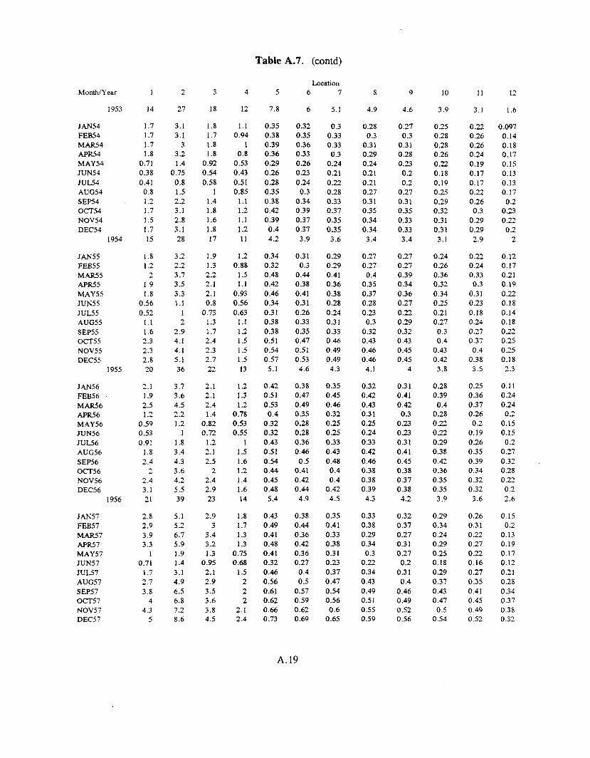
Monthly ear
1953
JAN54 FEB54 MAR54 APR54 MAY54 JUN54 JUL54 AUG54 SEP54 Om54 NOV54 DEC54
1954
JAN55 FEB55 MAR55 APR55 MAY55 JUN55 JUL55 AUG55 SEP55 O m 5 5 NOV55 DEC55
1955
JAN56
MAR56 APR-56 MAY56 JUN56 JUL56 AUG56 SEP56 Om56 NOV56 DEC56
FEB56 -
1956
JAN57 FEB57 MAR57 APR57 MAY57 JUN57 JUU7 AUG57 SEP57 Om57 NOV57 DEC57
1
14
1.7 1.7 1.7 1.8
0.71 0.38 0.41 0.8 1.2 1.7 1.5 1.7 15
1.8 1.2
2 1.9 1.8
0.56 0.52
1.1 1.6 2.3 2.3 2.8 20
2.1 1.9 2.5 1.2
0.59 0.53 0.91
1.8 2.4
2 2.4 3.1 21
2.8 2.9 3.9 3.3
1 0.71
1.7 2.7 3.8
4 4.3
5
2
27
3.1 3.1
3 3.2 1.4
0.75 0.8 1.5 2.2 3.1 2.8 3.1 28
3.2 2.2 3.7 3.5 3.3 1.1
1 2
2.9 4.1 4.1 5.1 36
3.7 3.6 4.5 2 2 1.2
1 1.8 3.4 4.3 3.6 4.2 5.5 39
5.1 5.2 6.7 5.9 1.9 1.4 3.1 4.9 6.5 6.8 7.2 8.6
3
18
1.8 1.7 1.8 1.8 0.92 0.54 0.58
1 1.4 1.8 1.6 1.8 17
1.9 1.3 2.2 2.1 2.1 0.8
0.73 1.3 1.7 2.4 2.3 2.7 22
2.1 2.1 2.4 1.4
0.82 0.72
1.2 2.1 2.5
2 2.4 2.9 23
2.9 3
3.4 3.2 1.3
0.95 2.1 2.9 3.5 3.6 3.8 4.5
4
12
1.1 0.94
1 0.8
0.53 0.43 0.51 0.85
1.1 1.2 1.1 1.2 11
1.2 0.88
1.5 1.1
0.93 0.56 0.63
1.1 1.2 1.5 1.5 1.5 13
1.2 1.3 1.2
0.78 0.53 0.55
1 1.5 1.6 1 2 1.4 1.6 14
1.8 1.7 1.3 1.3
0.75 0.68
1.5 2 2 2
2. I 2.4
Table A.7. (contd)
5
7.8
0.35 0.38 0.39 0.36 0.29 0.26 0.28 0.35 0.38 0.42 0.39 0.4 4.2
0.34 0.32 0.48 0.42 0.46 0.34 0.3 1 0.38 0.38 0.51 0.54 0.57 5.1
0.42 0.51 0.53 0.4
0.32 0.32 0.43 0.51 0.54 0.44 0.45 0.48 5.4
0.43 0.49 0.41 0.48 0.41 0.32 0.46 0.56 0.61 0.62 0.66 0.73
6
6
0.32 0.35 0.36 0.33 0.26 0.23 0.24 0.3
0.34 0.39 0.37 0.37 3.9
0.3 1 0.3
0.44 0.38 0.41 0.3 1 0.26 0.33 0.35 0.47 0.51 0.53 4.6
0.38 0.47 0.49 0.35 0.28 0.28 0.36 0.46 0.5
0.41 0.42 0.44 4.9
0.38 0.44 0.36 0.42 0.36 0.27 0.4 0.5
0.57 0.59 0.62 0.69
A. 19
Location 7
5.1
0.3 0.33 0.33 0.3
0.24 0.21 0.22 0.28 0.33 0.37 0.35 0.35 3.6
0.29 0.29 0.41 0.36 0.38 0.28 0.24 0.31 0.33 0.46 0.49 0.49 4.3
0.35 0.45 0.46 0.32 0.25 0.25 0.33 0.43 0.48 0.4 0.4
0.42 4.5
0.35 0.41 0.33 0.38 0.31 0.23 0.37 0.47 0.54 0.56 0.6
0.65
8
4.9
0.28 0.3
0.31 0.29 0.24 0.21 0.21 0.27 0.31 0.35 0.34 0.34 3.4
0.27 0.27 0.4
0.35 0.37 0.28 0.23 0.3
0.32 0.43 0.46 0.46 4.1
0.32 0.42 0.43 0.31 0.25 0.24 0.33 0.42 0.46 0.38 0.38 0.39 4.3
0.33 0.38 0.29 0.34 0.3 0.22 0.34 0.43 0.49 0.51 0.55 0.59
9
4.6
0.27 0.3
0.31 0.28 0.23 0.2 0.2
0.27 0.3 1 0.35 0.33 0.33 3.4
0.27 0.27 0.39 0.34 0.36 0.27 0.22 0.29 0.32 0.43 0.45 0.45 4
0.3 1 0.41 0.42 0.3
0.23 0.23 0.31 0.41 0.45 0.38 0.37 0.38 4.2
0.32 0.37 0.27 0.3 1 0.27 0.2
0.3 1 0.4
0.46 0.49 0.52 0.56
10
3.9
0.25 0.28 0.28 0.26 0.22 0.18 0.19 0.25 0.29 0.32 0.3 1 0.31 3.1
0.24 0.26 0.36 0.32 0.34 0.25 0.21 0.27 0.3 0.4
0.43 0.42 3.8
0.28 0.39 0.4
0.28 0.22 0.22 0.29 0.38 0.42 0.36 0.35 0.35 3.9
0.29 0.34 0.24 0.29 0.25 0.18 0.29 0.37 0.43 0.47 0.5
0.54
I 1
3.1
0.22 0.26 0.26 0.24 0.19 0.17 0.17 0.22 0.26 0.3
0.29 0.29 2.9
0.22 0.24 0.33 0.3
0.3 1 0.23 0.18 0.24 0.27 0.37 0.4
0.38 3.5
0.25 0.36 0.37 0.26 0.2
0.19 0.26 0.35 0.39 0.34 0.32 0.32 3.6
0.26 0.31 0.22 0.27 0.22 0.16 0.27 0.35 0.41 0.45 0.49 0.52
12
1.6
0.097 0.14 0.18 0.17 0.15 0.13 0.13 0.17 0.2 0.23 0.22 0.2
2
0.12 0.17 0.21 0.19 0.22 0.18 0.14 0.18 0.22 0.25 0 2 5 0.18 2.3
0.11 0.24 0.24 0.2
0.15 0.15 0.2
0.27 0.32 0.28 0.22 0.2 2.6
0.15 0.2
0.13 0.19 0.17 0.12 0.21 0.28 0.34 0.37 0.38 0.32

MonthlYear
1957
JAN58 FEB58 MAR58 APRs8 MAY58 JUN58 JUL58 AUG58 SEP58 Om58 NOV58 DEC58
1958
JAN59 FEB59 MAR59 Am59 MAY59 JUN59 JUL59 AUG59 SEP59 Om59 NOV59 DEC59
1959
JAN60 FEB60 MAR60 ApR60 MAY60 JUN60 JUL60 AUG60 SEP60 Om60 NOV60 DEC60
1960
JAN61 FEB6 1 MAR6 1 APR61 MAY61 JUN61 JUL61 AUG61 SEP6 1 Om61 NOV61 DEC61
I
36
4.9 4
3.2 2.9 1.6
1 1.9 2.9 3.7 4.4 4.1 4.5 39
3.2 3
3.5 3.1 1.5
0.91 1 3
2.7 2.3 3.4 4.5 32
6.2 5.2
7 3.6 2.8 1.3 1.4 3.4
5 4.8 8.2 6.7 56
8.3 3.9 5.7 4.2 2.3 0.92
1.7 2.5 2.2 3.4 3.9 4.3
2
63
8.1 7
5.6 5.3 2.9 1.9 3.4 5.2 6.1 7.5
7 7.8 68
5.4 5.3 6.1 5.4 2.8 1.7
2 5.1 4.8
4 5.9 7.9 57
11 8.7 12
6.4 5
2.5 2.6 5.8 8.5
8 13 11 94
14 7
9.9 7.5 4.3 1.7 3.1 4.4 3.8 5.6 6.3 6.8
3
35
4.2 3.7 3.2 3.1 1.9 1.3 2.2
3 3.2
4 3.6
4 38
2.8 2.9 3.5 3.2 1.9 1.2 1.4 3.1 2.9 2.4 3.4 4.2 33
5.7 4.5 5.7
4 3.3 1.8 1.8 3.4 4.4
4 6.5 5.5 51
6.8 3.9 5.3 4.4 2.7 1.2
2 2.5 2.1 2.7 3.1
3
4
19
2.1 1.7 1.7 1.5
1 0.97
1.6 2
1.8 2.3 1.8
2 21
1.4 1.7
2 1.7 1.3
0.87 1.2 2.1 1.9 1.5 2.1 2.5 20
3.3 2.3 2.5 2.4 1.9 1.3 1.5 2.3 2.4 2.2 3.2 2.8 28
3.4 2.1
3 2.5 1.7
1 1.5 1.7 1.3 1.4 1.6 1.4
Table A.7. (contd)
Location 5
6.2
0.45 0.56 0.48 0.58 0.47 0.39 0.45 0.5
0.37 0.61 0.56 0.56
6
0.31 0.48 0.53 0.48 0.47 0.4
0.41 0.38 0.53 0.39 0.57 0.69 5.6
1.1 0.6 0.6
0.72 0.64 0.52 0.53 0.43 0.52 0.54 0.61 0.78 7.5
0.87 0.72 0.88 0.94 0.63 0.5
0.33 0.48 0.51 0.44 0.49 0.39
6
5.6
0.4 0.51 0.42 0.52 0.41 0.32 0.38 0.45 0.34 0.57 0.52 0.51 5.3
0.27 0.43 0.47 0.41 0.38 0.33 0.33 0.3 1 0.48 0.34 0.51 0.63 4.9
0.99 0.57 0.55 0.58 0.53 0.43 0.43 0.36 0.48 0.51 0.56 0.73 6.7
0.8 0.66 0.81 0.87 0.55 0.42 0.27 0.45 0.49 0.43 0.47 0.37
A.20
7
5.2
0.37 0.46 0.39 0.47 0.36 0.27 0.35 0.42 0.32 0.54 0.49 0.48 4.9
0.25 0.4
0.43 0.37 0.33 0.27 0.29 0.29 0.46 0.32 0.48 0.6 4.5
0.94 0.55 0.51 0.51 0.47 0.37 0.39 0.33 0.46 0.49 0.54 0.7 6.3
0.75 0.63 0.76 0.82 0.5
0.36 0.24 0.43 0.48 0.42 0.45 0.36
8
4.8
0.31 0.4
0.34 0.43 0.34 0.25 0.32 0.38 0.29 0.48 0.45 0.43
4.4
0.22 0.36 0.39 0.34 0.3 1 0.26 0.27 0.26 0.42 0.29 0.45 0.55 4.1
0.86 0.51 0.46 0.47 0.43 0.35 0.36 0.3
0.42 0.45 0.48 0.63 5.7
0.67 0.57 0.7
0.77 0.47 0.34 0.22 0.4
0.44 0.39 0.41 0.33
9
4.5
0.28 0.38 0.32 0.41 0.3 1 0.23 0.29 0.35 0.27 0.45 0.43 0.4 4.1
0.2 0.33 0.37 0.32 0.28 0.23 0.24 0.24 0.4
0.27 0.42 0.52 3.8
0.81 0.5
0.43 0.43 0.4
0.32 0.33 0.28 0.4
0.43 0.46 0.6 5.4
0.63 0.55 0.66 0.75 0.44 0.31 0.2
0.38 0.43 0.38 0.4
0.33
10
4.2
0.25 0.36 0.29 0.38 0.29 0.2
0.26 0.33 0.26 0.42 0.4
0.37 3.8
0.18 0.3
0.34 0.3
0.25 0.2
0.22 0.22 0.38 0.26 0.39 0.5 3.5
0.77 0.49 0.41 0.39 0.37 0.29 0.3 1 0.26 0.37 0.41 0.44 0.56 5.1
0.58 0.52 0.62 0.72 0.42 0.29 0.18 0.36 0.42 0.37 0.38 0.32
11
3.9
0.23 0.33 0.27 0.36 0.26 0.17 0.24 0.31 0.24 0.4
0.39 0.35 3.5
0.16 0.28 0.32 0.28 0.22 0.17 0.19 0.2
0.37 0.24 0.37 0.47 3.3
0.72 0.48 0.39 0.36 0.33 0.26 0.28 0.24 0.35 0.4
0.42 0.53 4.8
0.53 0.5
0.59 0.69 0.4
0.25 0.16 0.35 0.41 0.36 0.36 0.32
12
2.9
0.098 0.19 0.19 0.26 0.21 0.12 0.18 0.25 0.21 0.3
0.27 0.24 2.5
0.085 0.17 0.24 0.21 0.16 0.12 0.14 0.16 0.31 0.2
0.29 0.37 2.5
0.48 0.35 0.25 0.25 0.25 0.2
0.23 0.19 0.29 0.34 0.28 0.34 3.4
0.31 0.33 0.37 0.56 0.34 0.19 0.14 0.28 0.37 0.34 0.26 0.21

Table A.7. (contd)
Location 7
6.2
0.47 0.46 0.55 0.67 0.48 0.42 0.5
0.62 0.99 0.6
0.43 0.5 6.7
0.25 0.28 0.26 0.34 0.22 0.21 0.19 0.19 0.18 0.23 0.24 0.23 2.8
0.19 0.27 0.31 0.32 0.36 0.29 0.21 0.21 0.25 0.19 0.24 0.22 3.1
0.21 0.19 0.25 0.25 0.23 0.21 0.15 0.14 0.14 0.14 0.14 0.17
MonthlYear
1961
1 AN62 FEB62 M AR62 APR62 MAY62 JUN62 JUL62 AUG62 SEP62 Om62 NOV62 DEC62
1962
JAN63 FEB63 MAR63 APR63 MAY63 JUN63 JUM3 AUG63 SEP63 Off63 NOV63 DEC63
1963
JAN64 FEB64 MAR64 APR64 MAY64 JUN64 JUL64 AUG64 SEP64 Om64 NOV64 DEC64
1964
JAN65 FEFi65 MAR65 APR65 MAY65 JUN65 JUMS AUG65 SEP65 Om65 NOV65 DEC65
1
43
4.4 3.9 5.8 5.5 2.5 1.6 1.8
3 4.8 3.8 2.9
3 43
2.5 2.6 4.5
4 1.7
1 1.4 2.3 3.3 3.4 3.8 4.5 35
4.6 3.1 4.1 4.3 2.9 1.1 1.2 2.2 3.2 2.4 4.1 4.5 38
3.1 2.3 2.9 2.6 1.2
0.88 0.91
1.4 2.1 2.9 2.4 2.6
2
74
7.2 6.6 9.5 9.5 4.6 3.1 3.3 5.3 8.1 6.4 4.9 5.2 74
4.2 4.4 7.6
7 3.1 1.9 2.5 3.9 5.4 5.5 6.1 7.3 59
7.2 5.3 6.8
7 5.2
2 2.1 3.8 5.3 4.1 6.7 7.3 63
5.2 4.1 5
4.5 2.2 1.7 1.7 2.4 3.6 4.7
4 4.3
3
40
3.5 3.3 4.5 5.2
3 2.1 2 .2 3.2 4.3 3.2 2.6 2.8 40
2.2 2.3 3.8 3.8 1.9 1.3 1.6 2.2 2.7 2.7 2.7 3.3 31
3.2 2.7 .3.2 3.4 3.1 1.4 1.4 2.3 2.7 2.2 3.3 3.3 32
2.5 2.1 2.6 2.5 1.5 1.1 1.1 1.5 1.8 2.2
2 2.1
4
23
1.8 1.7
2 2.3 1.7 1.5 1.7 2.3 2.6 1.6 1.3 1.5 22
1.2 1.1 1.8
2 0.93 0.89
1.2 1.5 1.4 1.4 1.3 1.5 16
1.4 1.4 1.5 1.3 1.5
0.91 1.1 1.5 1.4 1.3 1.7 1.4 16
1.1 0.92
1.2 1.1
0.86 0.73 0.79 0.99 0.95
1 0.99
1.1
5
7.2
0.53 0.5 0.6
0.81 0.64 0.58 0.61 0.7
1 0.61 0.47 0.56
7.7
0.29 0.33 0.32 0.42 0.3
0.31 0.29 0.24 0.21 0.26 0.27 0.26 3.5
0.23 0.32 0.35 0.38 0.49 0.43 0.34 0.28 0.29 0.23 0.28 0.27 3.9
0.26 0.26 0.32 0.33 0.34 0.31 0.23 0.19 0.17 0.17 0.17 0.2
6
6.6
0.49 0.48 0.58 0.73 0.54 0.47 0.54 0.65
1 0.61 0.45 0.53
7.1
0.27 0.3
0.28 0.37 0.25 0.24 0.22 0.2
0.19 0.24 0.25 0.24 3.1
0.21 0.29 0.33 0.34 0.41 0.35 0.25 0.23 0.26 0.2
0.25 0.24 3.4
0 .23 0.22 0.28 0.28 0.27 0.26 0.18 0.16 0.15 0.15 0.15 0.18
8
5.7
0.43 0.42 0.5
0.62 0.45 0.39 0.47 0.58 0.91 0.58 0.4
0.47 6.2
0.23 0.25 0.23 0.31 0.21 0.19 0.17 0.17 0.16 0.2
0.21 0.2 2.5
0.17 0.25 0.28 0.29 0.34 0.27 0.19 0.19 0 .23 0.17 0.22 0.19 2.8
0.18 0.17 0.23 0.23 0.22 0.2
0.14 0.13 0.13 0.12 0.13 0.15
9
5.5
0.41 0.42 0.48 0.59 0.42 0.36 0.45 0.56 0.88 0.58 0.39 0.45
6
0.22 0.24 0.22 0.29 0.19 0.17 0.15 0.15 0.15 0.18 0.2
0.19 2.3
0.15 0.23 0.26 0.28 0.31 0.24 0.16 0.17 0.22 0.16 0.2
0.18 2.6
0.16 0.16 0.22 0.22 0.2
0.17 0.12 0.11 0.12 0.11 0.12 0.14
10
5.2
0.38 0.4
0.46 0.55 0.39 0.33 0.43 0.54 0.85 0.58 0.37 0.43 5.7
0.2 0.23 0.2
0.27 0.18 0.15 0.13 0.14 0.14 0.17 0.19 0.18 2.2
0.14 0.22 0.25 0.26 0.28 0.21 0.14 0.16 0.2
0.16 0.18 0.17 2.4
0.15 0.15 0.2 0.2
0.18 0.16 0.11 0.1
0.1 1 0.1
0.1 1 0.13
11
4.9
0.36 0.39 0.44 0.54 0.36 0.3
0.41 0.52 0.82 0.59 0.36 0.42 5.5
0.19 0.22 0.19 0.25 0.16 0.12 0.11 0.13 0.13 0.16 0.18 0.17
2
0.12 0.2
0.23 0.25 0.25 0.17 0.12 0.15 0.19 0.15 0.16 0.16 2.2
0.14 0.14 0.19 0.19 0.15 0.13
0.096 0.094
0.1 0.097 0.099 0.12
12
3.7
0.25 0.33 0.3
0.43 0.29 0.23 0.35 0.46 0.68 0.5
0.26 0.3 4.4
0.14 0.16 0.14 0.17 0.12
0.086 0.082 0.099 0.11 0.14 0.19 0.12
1.6
0.042 0.14 0.16 0.19 0.19 0.12
0.074 0.1 1 0.18 0.13 0.11
0.086 1.5
0.069 0.1
0.15 0.16 0.1 1
0.093 0.07
0.074 0.08
0.078 0.075 0.09
A.21

Table A.7. (contd)
Location MonthlYear
1965
JAN66 FEB66 MAR66 APR66 MAY66 JUN66 JUL66 AUG66 SEP66 Om66 NOV66 DEC66
1966
JAN67 FEB67 MAR67 APR67 MAY67 JUN67 JUL67 AUG67 SEP67 Om67 NOV67 DEC67
1967
JAN68 FEB68 MAR68 APR68 MAY68 JUN68 JUL68 AUG68 SEP68 Om68 NOV68 DEC68
1968
JAN69 FEB69 MAR69 APR69 MAY69 JUN69 JUL69 AUG69 SEP69 Om69 NOV69 DEC69
1
25
2.5 2
2.5 2.3 1.3
0.71 0.27 0.65 2.5 2.3 2.2 2.6 22
2.5 2.3 2.1 2.5 1.9
0.53 0.7 1.4 1.9
2 1.8 1.8 21
1.8 2.2 1.7 1.7 1.4
0.48 0.46
1.1 1.2 1.5 1.5 1.3 16
1.1 0.92
1.3 0.77 0.51 0.54 0.54 0.97
1 0.86 0.69 0.87
2
43
4 3.4 4.2 3.8 2.3 1.3 0.5 1.1 4.2 3.8 3.6 4.3 36
4.1 3.8 3.6 4.3 3.4
1 1.3 2.5 3.2 3.3 3.1 3.1 37
3 3.7
3 2.9 2.4 0.9
0.84 2
2.1 2.6 2.5 2.3 28
1.9 1.6 2.3 1.4
0.95 1
0.97 1.7 1.7 1.5 1.2 1.5
3
23
1.8 1.7 2.1 1.9 1.4
0.91 0.33 0.61
2 1.8 1.7
2 18
2 1.8 1.9 2.3 1.8 0.7
0.89 1.5 1.6 1.7 1.6 1.6 19
1.4 1.7 1.6 1.6 1.4
0.61 0.56
1.2 1.1 1.3 1.2 1.2 1.5
1 0.97
1.3 0.89 0.63 0.67 0.62 0.94 0.85 0.74 0.61 0.82
4
12
0.83 0.89
1 0.79 0.88 0.7
0.27 0.38
1.1 0.97 0.85
1 9.7
0.99 0.92
1.1 1.2
0.85 0.51 0.71
1 0.99 0.87 0.8
0.91 11
0.75 0.77 0.91 0.86 0.72 0.42 0.44 0.75 0.67 0.68 0.62 0.66
8.3
0.53 0.58 0.64 0.52 0.38 0.46 0.45 0.61 0.47 0.41 0.36 0.49
5
3
0.13 0.15 0.19 0.19 0.25 0.21
0.065 0.04 0.18 0.25 0.2
0.21 2.1
0.21 0.23 0.28 0.31 0.27 0.26 0.24 0.2
0.22 0.19 0.17 0.19 2.8
0.12 0.17 0.21 0.2 0.2
0.15 0.12 0.15 0.13 0.12 0.12 0.12
1.8
0.1 0.13 0.16 0.18 0.14 0.14 0.1
0.12 0.082 0.074 0.065 0.084
6
2.5
0.12 0.13 0.17 0.17
0.2 0.16
0.048 0.033 0.16 0.24 0.19 0.2 1.8
0.19 0.21 0.26 0.29 0.23 0.22 0.19 0.17 0.2
0.17 0.16 0.17 2.5
0.1 0.15 0.18 0.13 0.12
0.071 0.056 0.085 0.086 0.073 0.081 0.079
1.2
0.054 0.077
0.1 0.092 0.064 0.057 0.048 0.073 0.065 0.055 0.049 0.059
7
2.2
0.1 1 0.12 0.15 0.15 0.17 0.13
0.041 0.03 0.16 0.23 0.19 0.19
1.7
0.18 0.2 0.25 0.27 0.21 0.18 0.17 0.16 0.19 0.17 0.15 0.16 2.3
0.096 0.14 0.17 0.11 0.1 1
0.053 0.043 0.071 0.078 0.065 0.073 0.068
1.1
0.043 0.067 0.084 0.071 0.046 0.039 0.037 0.063 0.064 0.05
0.049 0.053
8
2
0.1 0.11 0.14 0.14 0.16 0.12
0.037 0.026 0.14 0.21 0.18 0.17
1.5
0.16 0.19 0.23 0.25 0.2
0.17 0.15 0.14 0.18 0.15 0.14 0.15 2.1
0.085 0.12 0.15 0.11 0.1 0.05 0.04
0.067 0.075 0.061 0.068 0.065
1
0.04 0.064 0.079 0.067 0.043 0.036 0.035 0.059 0.06 1 0.047 0.046 0.051
9
1.9
0.091 0.1 1 0.13 0.13 0.14 0.1
0.032 0.023 0.13 0.2
0.17 0.16
1.4
0.15 0.18 0.22 0.24 0.18 0.16 0.14 0.13 0.17 0.15 0.13 0.14
2
0.077 0.12 0.14 0.11 0.1
0.048 0.039 0.065 0.074 0.06
0.066 0.064 0.96
0.038 0.063 0.077 0.065 0.041 0.035 0.034 0.058 0.061 0.046 0.046 0.05
10
1.7
0.083 0.1
0.12 0.13 0.13
0.091 0.028 0.021 0.12 0.19 0.17 0.16
1.3
0.14 0.18 0.21 0.23 0.17 0.14 0.12 0.12 0.16 0.14 0.12 0.13
1.9
0.07 0.1 1 0.13 0.11
0.099 0.046 0.037 0.063 0.072 0.059 0.064 0.064 0.92
0.037 0.06 1 0.075 0.063 0.039 0.033 0.033 0.056 0.06
0.046 0.045 0.049
11
1.5
0.074 0.096 0.11 0.12 0.12
0.075 0.024 0.02 0.11 0.19 0.16 0.15
1.3
0.13 0.17 0.2
0.22 0.16 0.12 0.11 0.12 0115 0.13 0.12 0.12
1.7
0.063 0.099 0.12 0.1
0.096 0.044 0.035 0.06
0.071 0.058 0.06 1 0.062 0.87
0.034 0.059 0 .OR 0.06
0.037 0.03
0.031 0.054 0.06 0.044 0.044 0.048
12
1.1
0.042 0.073 0.075 0.089 0.09
0.053 0.019 0.015 0.089 0.17 0.13
0.097 0.94
0.069 0.12 0.16 0.18 0.14
0.084 0.082 0.097 0.13 0.1 1
0.089 0.088
1.3
0.036 0.067 0.086 0.093 0.084 0.039 0.031 0.05 1 0.064 0.047 0.04 1 0.039 0.68
0 .OB 0.046 0.062 0.051 0.031 0.025 0.027 0.046 0.056 0.039 0.04
0.033
A.22

Table A.7. (contd)
Location 6 7 3 5 8 9 12 MonthlYenr 1 2 A 10 11
1969 10
JAN70 1.3 FEB7O 0.039 MAR70 0.19 APR70 0.69 MAY70 0.53 JUN70 0.32 JUL70 0.49 AUG7O 0.38 SEW0 0.85 Om70 0.87 NOV70 0.82 DEC70 0.82
1970 7.3
JAN71 0.75
18 10 5.9 1.4 0.79 0.67 0.63 0.61 0.6 0.57 0.48
2.2 0.093 0.34
1.2 0.92 0.57 0.87 0.66
1.4 1.5 1.4 1.4 13
1.2
1.1 0.069 0.17 0.64 0.51 0.37 0.55 0.38 0.74 0.77 0.72 0.73 6.7
0.59
0.53 0.035 0.09 0.34 0.23 0.19 0.33 0.25 0.41 0.42 0.38 0.37 3.6
0.25
0.067 0.014 0.021 0.079 0.078 0.069 0 .OS3 0.062 0.098 0.11 0.1
0.098 0.88
0.065
0.03 0.02 0.014 0.014 0.013 0.01 0.052 0.043 0.051 0.045 0.036 0.028 0.049 0.041 0.046 0.043 0.069 0.059 0.086 0.08 0.079 0.075 0.075 0.069
0.6 0.53
0.037 0.03
0.018 0.013
0.0094 0.04 0.044 0.027 0.039 0.041 0.055 0.076 0.071 0.065
0.5
0.026
0.017 0.013
0.0091 0.039 0.043 0.026 0.038 0.041 0.053 0.075 0.07
0.064 0.49
0.025
0.016 0.014
0.0086 0.038 0.043 0.025 0.037 0.04
0.052 0.074 0.069 0.063 0.48
0.024
0.014 0.014
0.0081 0.036 0.043 0.024 0.035 0.04 0.05
0.073 0.068 0.061 0.46
0.02.2
0.0065 0.01
0.0063 0.029 0.039 0.021 0.031 0.03 8 0.044 0.064 0.054 0.041 0.38
0.01 1
A.23

Table A.8. Occupational Representative Individual - Red Bone Marrow Equivalent Dose
Yeat
Cum. Dose
1950
1951
1952
1953
1954
1955
1956
1957
1958
1959
1960
1961
1962
1963
1964
1965
1966
1967
1968
1969
1970
1971
1
423
4.8
4.7
7
9.7
10
14
15
27
29
27
47
38
38
30
32
22
19
19
14
8.8
6.3
0.64
(millirem per year)
Location 2
73 1
9.6
9.2
13
18
19
25
27
46
51
48
80
65
66
50
53
37
32
32
25
15
11
1
3
405
6.6
6.2
9.1
12
11
15
16
25
28
28
43
36
36
26
27
20
16
17
13
8.8
5.7
0.5
4
234
4.6
4.5
6.4
7.8
7.1
9
9.6
14
16
17
24
21
20
14
14
10
8.9
9.9
7.4
5.3
3.1
0.22
5
98
3.8
3.5
4.8
5.4
3.8
4.6
4.8
6.1
6.5
6.1
8.6
8.9
8.9
4.1
4.3
3.3
2.6
3.4
2.3
1.6
1
0.079
6
89
3.2
2.8
3.8
4.3
3.6
4.4
4.6
5.8
6.1
5.6
8
8.5
8.4
3.8
4
3
2.5
3.2
1.8
1.2
0.81
0.054
7
84
3
2.5
3.4
3.8
3.5
4.3
4.4
5.6
5.8
5.3
7.7
8.2
8.1
3.6
3.7
2.8
2.3
3
1.7
1
0.74
0.044
8
79
2.8
2.4
3.2
3.6
3.3
4.1
4.2
5.2
5.4
5
7.2
7.6
7.6
3.3
3.5
2.6
2.2
2.9
1.6
0.97
0.69
0.039
9
77
2.7
2.3
3.1
3.4
3.3
4
4.1
5.1
5.2
4.8
6.9
7.4
7.4
3.2
3.3
2.5
2.1
2.8
1.6
0.96
0.68
0.038
10
73
2.5
2.1
2.7
3
3.2
3.9
4
4.9
5
4.6
6.7
7.1
7.2
3
3.2
2.3
2
2.6
1.5
0.93
0.67
0.035
11
70
2.3
1.8
2.4
2.7
3.1
3.8
3.8
4.8
4.8
4.4
6.4
6.9
7
2.9
3
2.2
1.9
2.5
1.5
0.9
0.65
0.032
12
53
1.8
1.3
1.8
1.7
2.4
2.7
2.9
3.7
3.6
3.5
4.8
5.3
5.7
2.3
2.3
1.8
1.5
2
1 .1
0.76
0.53
0.017
A.24

Table A.9. Occupational Representative Individual - Lower Large Intestine Equivalent Dose
Year
Cum. Dose
1950
1951
1952
1953
1954
1955
1956
1957
1958
1959
1960
1961
1962
1963
1964
1965
1966
1967
1968
1969
1970
1971
(millirem per year)
Location 1
1420
44
37
49
66
69
83
86
130
130
77
120
94
82
71
80
55
38
41
33
20
15
1.7
2
2710
90
75
99
130
130
160
I70
250
250
150
230
170
150
130
150
100
69
76
62
37
29
3.1
3
1700
64
54
72
91
87
100
110
150
150
93
140
100
93
79
88
61
40
45
37
23
18
1.7
4
1080
45
40
52
63
57
68
'68
91
91
61
86
65
56
48
50
35
24
28
23
15
11
0.81
5
443
38
34
43
44
21
24
24
28
27
21
26
21
21
14
15
12
6.5
9
7.2
4.9
3.2
0.24
6
368
32
28
35
35
18
20
21
24
23
18
22
18
18
12
13
9.9
5.6
7.9
4.2
2.4
1.5
0.093
7
328
28
25
30
31
16
18
19
21
20
16
20
17
17
11
12
8.9
5.1
7.2
3.3
1.7
1.1
0.06
8
303
27
24
29
29
16
18
18
19
17
15
18
15
15
9.3
10
7.9
4.5
6.4
3
1.6
0.99
0.052
9
279
25
23
27
28
15
17
17
17
15
13
16
13
14
8.1
9.1
7
4
5.7
2.7
1.5
0.94
0.049
10
245
22
19
23
24
13
15
15
15
13
12
14
12
13
7.1
8
6.3
3.6
5.2
2.5
1.4
0.9
0.045
11
205
17
16
17
18
11
13
13
13
11
10
12
11
12
6.2
6.9
5.4
3.2
4.5
2.2
1.3
0.85
0.04
12
115
8.2
7.2
8
7.8
6.4
6.7
7.5
7.4
6.6
6.4
7.6
7.1
8.1
3.9
4.2
3.5
2.1
3
1 .5
1
0.65
0.019
A.25

Appendix B
Summary of Technical Steering Panel Comments and Battelle, Pacific Northwest Laboratories Responses

Appendix B
Summary of Technical Steering Panel Comments and Battelle, Pacific Northwest Laboratories Responses
Document Title: Columbia River Pathwav Dosimetry ReDort. 1944-1992
Document Number: PNWD-2227 HEDR Summary Comments by: D.S. Barth
The comments received from various members of the TSP on the subject report are all included as an attachment to this summary. Many of the comments are essentially editorial in nature in that they recommend changes which will improve the clarity of the report. These should be carefully considered and responded to by making appropriate changes or by rebutting the comments.
There are several substantive comments which are believed to be of greater importance. Of these, the ones believed to be of highest priority are summarized below.
Some explanation is needed as to why there is a displacement in time of the peak years for Na-24, Np-239, and Ar-76.
Another chart should be added depicting cumulative doses from the river at the 12 locations listed in Appendix A. 1 for the time period 1944-1992.
A clearer discussion is needed explaining how concentration and the amount of water in the river leads to an estimate of neutron-induced radioisotope inventory in the river.
The term "measured doses" needs to be adequately defined.
The User's Guide prepared as a separate document should be included in the report. Response: NA - This comment does not appear in the list of numbered comments and so is responded to here. A user's guide for the Atmospheric Pathway Dosimetry Report, 1944-1992 (PNWD-2228 HEDR) was presented at the Technical Steering Panel public meeting held April 1994 and will be included as an appendix in the final publication of that report. However, a user's guide for the Columbia River Pathway Dosimetry Reporr, 1944-1992 was not created because understanding the dose estimates for that pathway was not complex. Both D.S. Barth (TSP member who summarized the comments) and M.L. Blazek (TSP Chair) have agreed that no action should be taken on this comment.

Summary of Technical Steering Panel Comments and Battelle, Pacific Northwest Laboratories Responses
Comment Number Commenter
TSP Comments:
Page, Paragraph Comment Summary
1 W. Bishop N J . Gerrnond
Full Report Reviewed, no specific comments.
2 J. Till
3
4
B. Shleien
B. Shleien
Full Report This is an excellent report. My only comment is the difficulty one has in extracting dose information from it. With the air pathway, we have maps. Could we include additional graphics that help the reader better understand the doses for a given scenario@).
I have previously had an opportunity to review this document during a visit to the Hanford Site and relayed my comments verbally to the Battelle staff. It appears that all were
report, with the exceptions noted below.
Full Report
incorporated into this draft
General Comment The term "occupational representative individual" is confusing. 1 suggest "commercial boat or fishing individual." Previously, I commented on the term 50- percent subjective confidence interval. I still do not understand how or why the term "subjective" is employed.
Resolution
NA.
Figure S.2 added to show the cumulative dose for the three representative individuals at the twelve locations.
NA - Thank YOU.
The term "occupational representative individual" was retained but the definition clarified. Text modified.
N A = Noaction. B.2

Summary of Technical Steering Panel Comments and Battelle, Pacific Northwest Laboratories Responses
Comment Number Commenter
5 M. Robkin
10
G. Roessler
G. Roessler
G. Roessler
G. Roessler
G. Roessler
Page. ParamaDh Comment Summan
Pg vi The phrase "measured doses" begs the question, how were these doses "measured." Are they the result of total population whole-body counting, etc., or based on some calculation? The word "measured" is sufficiently strong to require better documentation than is given in section 4.1.4 which only refers to estimates to a maximum representative individual (i.e., calculation based on assumptions). "Ingested" is a nice word, but better communication with the variety of readers will be had by using "ate".
Pg vii, Figure Y axis, use (mrem not mremlyr) as the X axis is the year.
Pg xiv Effective dose equivalent @DE) - suggest value used to account for the fact that a rem of radiation to one part of the body does not have the same potential health impact as a rem of dose to another part. It is the sum of the dose to all parts of the body from internal deposition of radionuclides and the dose from external radiation exposure.
neutron flux: rate of neutron bombardment per unit cross- sectional area.
Pg 3.4, Para 1, Why were gallium-72 and Line 5 ym'lum-90 included? Text
doesn't explain.
Pg xv
Pg 3.5, Para 2, After activation of naturally Line 2 occurring uranium-238 put
(neutron capture products)
Resolution
Agree. "Measured" has been changed to "estimated." Ingested was retained as it has been standard usage throughout HEDR documents.
NA - The graphs present average dose rates in a given year.
Agree. Definition modified.
Agree. Definition modified.
Gallium-72 and ymium-90 were included because of public interest. Text modified.
Text modiiied.
NA = No action. B.3

Summary of Technical Steering Panel Comments and Battelle, Pacific Northwest Laboratories Responses
Comment Number Commenter Page, Paragraph
11 M. Robkin Pg 3.5, sec 3 . 1 . 1 . ~ 3
12
13
14
G. Roessler Pg 3.6, Para 1, Line 3
G. Roessler Pg 3.6, Para 1, Line 9
M. Robkin Pg 3.6, Sec 3 . 1 . 2 : ~ ~ 2
Comment Summary
Probably the actual holdup time in the retention basin is known to no better than one significant figure. Why not refer to holdup t i m a BS 2 - 4 hours?
Bred actinides has not been used before. Suggest you call it uranium-238 activation products. modified.
Instead of neutron capture product of uranium-238, it would be more complete to say: a decay product of uranium-239 which is a neutron capture product of uranium-238.
The sentence dealing with the 3,500 curies of sodium-24 would not be understood by the general reader. There is no discussion of how the amount of sodium-24 would be determined from concentration measurements. A clearer discussion is needed explaining how concentration and the amount of water in the river leads to an estimate of inventory in the river. Similarly, the discussion of zinc45 will be mysterious to the general reader. If the discussion is going to address issues of buildup and decay, more explanation is in order.
Resolution
The holdup time was modeled as 2.4-4.0 hours. Text modified.
Text modified
Text modified.
Text modified.
N A = Noaction. B . 4

Comment Number
15
16
17
Summary of Technical Steering Panel Comments and Battelle, Pacific Northwest Laboratories Responses
Commenter Page, Paragraph Comment Summary
M. Robkin . Pg 3.7, Fig 3.2 Some explanation is needed as to why there is a displacement in time of the peak years for Na-24, Np239, and As-76. The other two nuclides are at too low of a level to discuss peaks. These are all basicallyactivationproducts, and their release rates should be correlated in time unless there was some remarkable time varying shift in water chemistry that caused these three elements to peak at different years. Note that the time shift in the representative individual’s dose at Richland is well explained in section 4.4.3. An equally convincing explanation is needed in section 3.1.2.
G. Roessler Pg 3.9 Celilio should be spelled Celilo on the map.
We have lot of wood ducks around our place. They tell me that they prefer their name to be spelled with two words.
G. Roessler Pg 3.14, Last Para, Line4
Resolution
NA - Section 3.1.2 shows the source term used to estimate dose. The source term report (Heeb and Bates 1994, p.4.11) contains the reasons for the displacement.
corrected.
corrected.
NA = Noaction. B.5
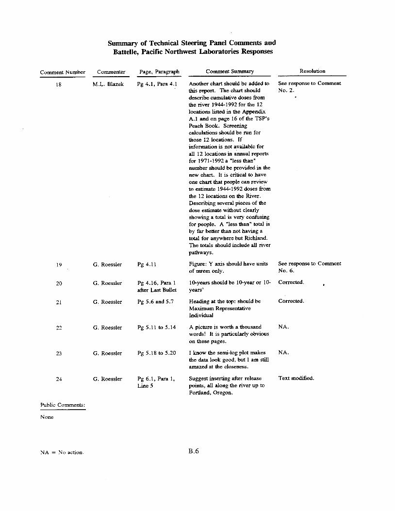
Summary of Technical Steering Panel Comments and Battelle, Pacific Northwest Laboratories Responses
Comment Number Commenter
18 M.L. Blazek
19
20
21
22
23
24
G. Roessler
G. Roessler
G. Roessler
G. Roessler
G. Roessler
G. Roessler
Page, Paragraph Comment Summaxy
Pg 4.1, Para 4.1
Pg 4.11
Pg 4.16, Para 1 after Last Bullet
Pg 5.6 and 5.7
Pg 5.11 to 5.14
Pg 5.18 to 5.20
Pg 6.1, Para 1, Line 5
Another chart should be added to this report. The chart should describe cumulative doses from the river 1944-1992 for the 12 locations listed in the Appendix A.1 and on page 16 of the TSP's Peach Book. Screening calculations should be run for those 12 locations. If information is not available for all 12 locations in annual reports for 1971-1992 a "less than" number should be provided in the new chart. It is critical to have one chart that people can review to estimate 1944-1992 doses from the 12 locations on the River. Describing several pieces of the dose estimate without clearly showing a total is very confusing for people. A "less than" total is by far better than not having a total for anywhere but Richiand. The totals should include all river pathways.
Figure: Y axis should have units of mrem only.
1 @years should be 1 &year or 10- Y='
Heading at the top: should be Maximum Representative Individual
A picture is worth a thousand words! It is particularly obvious on these pages.
I know the semi-log plot makes the data look good, but 1 am still amazed at the closeness.
Suggest inserting after release points, al l along the river up to Portland, Oregon.
Resolution
See response to Comment No. 2.
See response to Comment No. 6.
corrected. *
corrected.
NA.
NA.
Text modified.
Public Comments:
None
N A = N o action. B.6

PNWD-2227 HEDR UC-000
Distribution
No. of Copies
Offsite
Technical Steering Panel
D. S . Barth University of Nevada 4505 Maryland Parkway Las Vega, NV 89154
W. A. Bishop P.O. Box 47651 Olympia, WA 98504-7651
M. L. Blazek Oregon Department of Energy 625 Marion Street N.E. Salem, OR 97310
G. G. Caldwell Tulsa City-County Health Dept. 4616 East 15th Street Tulsa, OK 74112
S . N. Davis Dept. of Hydrology and Water Resources Building 11 University of Arizona Tucson, AZ 85721
N . J . Germond 224 Iron Mountain Blvd. Lake Oswego, OR 97034
P. C. Klingeman Civil Engineering Dept. Apperson Hall 202 Oregon State University Corvallis, OR 9733 1-2302
No. of Copies
K. J . Kopecky Fred Hutchinson Cancer Research Center 1124 Columbia Street Seattle, WA 98104
P. D. McGavran Dept. of Health and Welfare 450 W. State Street, 4th Floor Boise, ID 83720-5450
R. L. Morrill Dept. of Geography, DP-10 University of Washington Seattle, WA 98195
A. H. Murphy 31 15 NW McKinley Drive - Corvallis, OR 97330
D. W. Price Agricultural Economics Hulbert Hall Room 211 Washington State University Pullman, WA 9916443210
M. A. Robkin Radiological Sciences, SB-75 University of Washington Seattle. WA 98195
G . S . Roessler Route 1, Box 139H Elysian, MN 56028
B. Shleien 2421 Homestead Drive Silver Springs, MD 20902
Distr. I

PNWD-2227 HEDR u c-000
No. of Copies
No. of Copies
A . P. Slickpoo, Sr. 809 Nez Perce Lane P.O. Box 31 1 Kamiah, ID 83536
J . E. Till Route 2 Box 122 Neeses, SC 29107
D. E. Walker, Jr. P.O. Box4147 Boulder, CO 80306
Other
2 DOE Office of Scientific and
Technical Information Center P.O. Box 62 Oak Ridge, TN 37830
Technical Information
B. Aripa Environmental Trust Colville Conferated Tribes P.O. Box 150 Nespelem, WA 99155
D. M. Beck U . S . Department of Energy 1000 Independence Avenue Room 5B301, M.S. EM-5 Washington, D.C. 20585
D. Bonga Kalispel Tribe P.O. Box 39 Usk, WA 99180
B. G. Brooks, EH-421 Room J-112 U . S . Department of Energy Germantown, MD 20545
18 K. CharLee Technical Support and
Public Information P.O. Box 47651 Olympia, WA 98504-765 1
J. P. Corley 2213 Torbett Richland, WA 99352
L. E. Denham Centers for Disease Control
4770 Buford Highway N.E., F-35 and Prevention
Atlanta, GA 30341 -3724
DNR Hanford Projects Attn: J. R. Wilkinson Confederated Tribes of the Umatilla
Indian Reservation P.O. Box638 Pendleton, OR 97801
M. R. Donnelly Public Health Service Centers for Disease Control
and Prevention 2201 Sixth Avenue, RX-22 Seattle, WA 98121
D. Ernst Planning Department Spokane Tribe P.O. Box 100 Wellpinit, WA 99040
L. L. German 2245 Oxford Road Columbus, OH 43221
Distr.2
No. of Copies
PNWD-2227 HEDR uc-000
No. of copies
H. A. Haerer Golder Associates, Inc. 4104 148th N.E. Redmond, WA 98052
R. Jim Confederated Tribes and Bands of the
Yakima Indian Nation P.O. Box 151 Toppenish, WA 98948
D. Powaukee Nez Perce Tribe P.O. Box 365 Lapwai, ID 83540
M. Queahpama Vital Statistics Confederated Tribes of the Warm Spring Reservation P.O. BoxC Warm Springs, OR 97761
M. C. Richmond Department of Civil and
Environmental Engineering Washington State University Pullman, WA 99164-2910
L. Seyler Coeur d’Alene Tribe Plummer, ID 83851
J. C . Simpson Golder Associates, Inc. 4104 148th N.E. Redmond, WA 98052
M. Squeochs Confederated Tribes and Bands of the
Yakima Indian Nation P.O. Box 151 Toppenish, WA 98948
L. Stembridge HEAL 1408 West Broadway Avenue Spokane, WA 99201-1902
W. L. Templeton 233 1 Enterprise Drive Richland, WA 99352
J. P. Thomas HHIN Resource Center 1719 Smith Tower 506 Second Avenue Seattle, WA 98104
Onsite
6 DOE Richland Operations Office
R. F. Brich, TSD A5-55 Public Reading Room (5) H2-53
42 Battelle, Pacific Northwest Laboratories
D. M. Anderson G. L. Black (5) S . D. Cannon D. E. Deonigi P. W. Eslinger W. T. Farris (10) M. D. Freshley R. 0. Gilbert W. A. Glass (2) S. P. Gydesen G. L. Harvey C. M. Heeb T. A. Ikenberry R. E. Jaquish E. B. Liebow B. A. Napier J . V. Ramsdell D. B. Shipler
K8-15 B 1-34 B 1-34 K8-11 B 1-34 K3-54 K6-77 K7-34 K3-53 P8-55 K2-02 K8-34 K3-54 B 1-34
HARC K3-54 K6-55 B 1-34
Distr.3
No. of Copies
S . F. Snyder S . A. Stage M. E. Thiede W. H. Walters
PNWD-2227 HEDR uc-ooo
No. of Copies
K3-54 J . R. Weber K3-53 K6-55 Publishing Coordination K1-06 K6-52 Records Center (2) K3-70 K6-60 Technical Library (2) P8-55
Distr.4