vysoke u´ cenˇ ´i technick e v brn´ eˇ · abstrakt pˇredloˇzen´a disertaˇcn´ı pr´ace se...
TRANSCRIPT

VYSOKE UCENI TECHNICKE V BRNEBRNO UNIVERSITY OF TECHNOLOGY
FAKULTA INFORMACNICH TECHNOLOGIIUSTAV POCITACOVE GRAFIKY A MULTIMEDIIFACULTY OF INFORMATION TECHNOLOGYDEPARTMENT OF COMPUTER GRAPHICS AND MULTIMEDIA
MODELOVANI PROZODICKYCH PRIZNAKU PROOVEROVANI MLUVCIHO V POD-PROSTORECHSUBSPACE MODELING OF PROSODIC FEATURES FOR SPEAKER VERIFICATION
DISERTACNI PRACEPHD THESIS
AUTOR PRACE Dipl.-Ing. MARCEL KOCKMANNAUTHOR
VEDOUCI PRACE Doc. Dr. Ing. JAN CERNOCKYSUPERVISOR
BRNO 2011


Abstract
The thesis investigates into speaker verification by means of prosodic features. This in-cludes an appropriate representation of speech by measurements of pitch, energy and du-ration of speech sounds. Two diverse parameterization methods are investigated: the firstleads to a low-dimensional well-defined set, the second to a large-scale set of heterogeneousprosodic features. The first part of this work concentrates on the development of so calledprosodic contour features. Different modeling techniques are developed and investigated,with a special focus on subspace modeling. The second part focuses on a novel sub-space modeling technique for the heterogeneous large-scale prosodic features. The modelis theoretically derived and experimentally evaluated on official NIST Speaker RecognitionEvaluation tasks. Huge improvements over the current state-of-the-art in prosodic speakerverification were obtained. Eventually, a novel fusion method is presented to elegantlycombine the two diverse prosodic systems. This technique can also be used to fuse thehigher-level systems with a high-performing cepstral system, leading to further significantimprovements.
Keywords
speaker verification, prosody, Gaussian mixture models, channel compensation, Joint fac-tor analysis, total variability model, iVector, probabilistic linear discriminant analysis,SNERFs, subspace multinomial model, iVector fusion
Bibliographic citation
Marcel Kockmann: Subspace modeling of prosodic features for speaker verification, Doctoralthesis, Brno University of Technology, Faculty of Information Technology, Brno, 2011.
iii


Abstrakt
Predlozena disertacnı prace se zabyva overovanım mluvcıho pomocı prozodickych prıznakuzahrnujıcıch hodnoty zakladnıho tonu, energie a delek recovych useku. Studovali jsme dverozdılne techniky pro parametrizaci: prvnı vede k dobre definovane sade mensıho poctuprıznaku, druha k vysoko-dimenzionalnı sade heterogennıch prozodickych prıznaku. Prvnıcast prace se venuje vyvoji prıznaku reprezentujıcıch prozodicke kontury, zde jsme vyvinulia overili nekolik modelovacıch technik, s durazem na modelovanı v reprezentativnıch pod-prostorech. Druha cast prace se zameruje na nove pod-prostorove modelovacı techniky proheterogennı prozodicke parametry s velkou dimenzionalitou. Model je teoreticky odvozena experimentalne overen na oficialnıch datech z NIST evaluacı overovanı mluvcıho (NISTSpeaker Recognition Evaluation). Ve srovnanı s ostatnımi soucasnymi prozodickymi jsmedosahli podstatne lepsıch vysledku. Na konci prace presentujeme take novou techniku proelegantnı kombinaci dvou prozodickych systemu. Tato technika muze byt pouzita rovnvezpro fuzi prozodickeho systemu se standardnım presnym cepstralnım systemem, coz vede kdalsımu podstatnemu zvysenı uspesnosti verifikace.
Klıcova slova
Overovanı mluvcıho, prozodie, modely smesı Gaussovskych rozdelenı, kompenzace prenosovehokanalu, Joint factor analysis, model totalnı variability, iVector, pravdepodobnostnı linearnıdiskriminacnı analyza, SNERFs, multinomialnı pod-prostorovy model, fuze iVectoru.
Bibliograficka citace
Marcel Kockmann: Modelovanı prozodickych prıznaku pro overovanı mluvcıho v pod-prostorech,Disertacnı prace, Vysoke ucenı technicke v Brne, Fakulta informacnıch technologiı, Brno, 2011.
v


Prohlasenı
Prohlasuji, ze jsem tuto disertacnı praci vypracoval samostatne pod vedenım Doc. Dr. Ing.Jana Cernockeho a Ing. Lukase Burgeta, Ph. D.. Uvedl jsem vsechny literarnı pramenya publikace, ze kterych jsem cerpal. Nektere systemy pouzite v praci byly vytvorenycleny vyzkumne skupiny Speech@FIT samostatne, nebo ve spolupraci s tretımi stranami(Agnitio, CRIM, SRI Internatioinal).
vii


Acknowledgements
First, I would like to thank my former colleagues at Siemens Speech Processing Group, es-pecially Stephan and Bernt. Without their idea to contact Honza for the PhD supervision,I wouldn’t have had the opportunity to do my research in such a great speech group.
I would like to thank everybody in Speech@FIT in Brno, especially Lukas and Honza.Although Honza is the only official supervisor, I have to thank them both equally, Lukasfor doing a great job in the technical supervision and Honza for organizing everything andkeeping the group running on such a high level. Not to mention all the social events.
Further, I have to thank my colleagues at SVOX, especially Georg who always gaveme the freedom to do my research on speaker verification and to attend conferences andworkshops.
Also, I thank all the great people I met at conferences and workshops like BOSARISfor the valuable input to my work. Especially, I have to thank Luciana from SRI, for thegreat collaborative work on prosodic features.
Last but not least, I thank my family and friends for the support and patience theygave me during the last years when I was somewhere between Munich and Brno.
Munich, November 2011
Marcel Kockmann
ix


Contents
List of Abbreviations xiii
1 Introduction 11.1 Automatic speaker verification . . . . . . . . . . . . . . . . . . . . . . . . . 31.2 Levels of information in speaker verification . . . . . . . . . . . . . . . . . 41.3 State-of-the-art . . . . . . . . . . . . . . . . . . . . . . . . . . . . . . . . . 5
1.3.1 Evolution of low-level speaker verification systems . . . . . . . . . . 51.3.2 Evolution of prosody-based speaker verification systems . . . . . . . 9
1.4 Motivation and contribution . . . . . . . . . . . . . . . . . . . . . . . . . . 121.4.1 Claims of the thesis . . . . . . . . . . . . . . . . . . . . . . . . . . . 121.4.2 Content of the thesis . . . . . . . . . . . . . . . . . . . . . . . . . . 13
2 Evaluation metrics and data 152.1 Evaluation metrics . . . . . . . . . . . . . . . . . . . . . . . . . . . . . . . 15
2.1.1 DET plots . . . . . . . . . . . . . . . . . . . . . . . . . . . . . . . . 152.1.2 Equal Error Rate . . . . . . . . . . . . . . . . . . . . . . . . . . . . 162.1.3 Detection Cost Function . . . . . . . . . . . . . . . . . . . . . . . . 16
2.2 Databases . . . . . . . . . . . . . . . . . . . . . . . . . . . . . . . . . . . . 182.2.1 Switchboard, NIST SRE 2004 and 2005 . . . . . . . . . . . . . . . . 182.2.2 NIST SRE 2006 . . . . . . . . . . . . . . . . . . . . . . . . . . . . . 192.2.3 NIST SRE 2008 . . . . . . . . . . . . . . . . . . . . . . . . . . . . . 192.2.4 NIST SRE 2010 . . . . . . . . . . . . . . . . . . . . . . . . . . . . . 20
3 Parameterization of speech for prosodic speaker verification 213.1 Prosodic contour features . . . . . . . . . . . . . . . . . . . . . . . . . . . . 21
3.1.1 Basic prosodic features . . . . . . . . . . . . . . . . . . . . . . . . . 223.1.2 Suprasegmental units . . . . . . . . . . . . . . . . . . . . . . . . . . 243.1.3 Contour approximation . . . . . . . . . . . . . . . . . . . . . . . . . 263.1.4 Final feature vector . . . . . . . . . . . . . . . . . . . . . . . . . . . 273.1.5 Experiments . . . . . . . . . . . . . . . . . . . . . . . . . . . . . . . 27
3.2 Syllable-based NERFs (SNERFs) . . . . . . . . . . . . . . . . . . . . . . . 313.2.1 Basic SNERFs . . . . . . . . . . . . . . . . . . . . . . . . . . . . . 333.2.2 SNERFs tokens . . . . . . . . . . . . . . . . . . . . . . . . . . . . . 343.2.3 Final SNERFs . . . . . . . . . . . . . . . . . . . . . . . . . . . . . . 343.2.4 Parameterization of SNERFs . . . . . . . . . . . . . . . . . . . . . 34
4 Modeling approaches for prosodic speaker verification 374.1 Standard UBM-GMM with MAP adaptation . . . . . . . . . . . . . . . . . 384.2 Introducing Joint Factor Analysis models . . . . . . . . . . . . . . . . . . . 414.3 Subspace models for parameters of Gaussian distributions . . . . . . . . . . 42
4.3.1 Separate speaker and channel subspaces . . . . . . . . . . . . . . . 42
xi

CONTENTS
4.3.2 Total variability subspace . . . . . . . . . . . . . . . . . . . . . . . 464.3.3 Probabilistic Linear Discriminant Analysis . . . . . . . . . . . . . . 504.3.4 Experiments . . . . . . . . . . . . . . . . . . . . . . . . . . . . . . . 53
4.4 Subspace models for parameters of multinomial distributions . . . . . . . . 564.4.1 Total variability subspace . . . . . . . . . . . . . . . . . . . . . . . 574.4.2 Experiments . . . . . . . . . . . . . . . . . . . . . . . . . . . . . . . 62
5 Final comparative study 675.1 Results for prosodic systems . . . . . . . . . . . . . . . . . . . . . . . . . . 67
5.1.1 System descriptions . . . . . . . . . . . . . . . . . . . . . . . . . . . 675.1.2 tel-phn:tel-phn condition . . . . . . . . . . . . . . . . . . . . . . . . 705.1.3 int-mic:tel-phn condition . . . . . . . . . . . . . . . . . . . . . . . . 725.1.4 int-mic:int-mic condition . . . . . . . . . . . . . . . . . . . . . . . . 725.1.5 Final observations . . . . . . . . . . . . . . . . . . . . . . . . . . . . 75
5.2 Calibration . . . . . . . . . . . . . . . . . . . . . . . . . . . . . . . . . . . 775.3 Combination with cepstral baseline system . . . . . . . . . . . . . . . . . . 81
5.3.1 tel-phn:tel-phn condition . . . . . . . . . . . . . . . . . . . . . . . . 815.3.2 tel-phn:int-mic condition . . . . . . . . . . . . . . . . . . . . . . . . 825.3.3 int-mic:int-mic condition . . . . . . . . . . . . . . . . . . . . . . . . 835.3.4 Final observations . . . . . . . . . . . . . . . . . . . . . . . . . . . . 84
6 Conclusions 856.1 Summary . . . . . . . . . . . . . . . . . . . . . . . . . . . . . . . . . . . . 85
6.1.1 Extraction of prosodic contour features . . . . . . . . . . . . . . . . 856.1.2 Modeling for prosodic contour features . . . . . . . . . . . . . . . . 866.1.3 Modeling for SNERFs . . . . . . . . . . . . . . . . . . . . . . . . . 866.1.4 iVector fusion . . . . . . . . . . . . . . . . . . . . . . . . . . . . . . 87
6.2 Current state and future work . . . . . . . . . . . . . . . . . . . . . . . . . 886.2.1 Prosodic feature extraction . . . . . . . . . . . . . . . . . . . . . . . 886.2.2 Prosodic modeling . . . . . . . . . . . . . . . . . . . . . . . . . . . 89
References 91
A Derivation of a Joint Factor Analysis Model 99A.1 Likelihood of data for a GMM model . . . . . . . . . . . . . . . . . . . . . 99A.2 Likelihood of data for a JFA model . . . . . . . . . . . . . . . . . . . . . . 100A.3 Posterior distribution of the hidden variable . . . . . . . . . . . . . . . . . 101A.4 EM Estimation of low rank matrices V and U . . . . . . . . . . . . . . . . 102
B Derivation of a Subspace Multinomial Model 105
xii

List of Abbreviations
ABC Agnitio-Brno-CRIM
ASR Automatic Speech Recognition
BFGS Broyden-Fletcher-Goldfarb-Shanno
BUT Brno University of Technology
DCF Detection Cost Function
DCT Discrete Cosine Transformation
DET Detection Error Tradeoff
DNA DesoxyriboNucleic Acid
DP Dynamic Programming
DTW Dynamic Time Warping
DVD Digital Versatile Disc
EER Equal Error Rate
EM Expectation-Maximization
F0 Fundamental frequency
FA Factor Analysis
GD Gradient Descent
GMM Gaussian Mixture Model
GSM Global System for Mobile Communications
HA Hessian approximation
IDCT Inverse Discrete Cosine Transformation
IRLS Iterative Reweighted Least Squares
JFA Joint Factor Analysis
JHU Johns Hopkins University
LDA Linear Discriminant Analysis
LLR Log-Likelihood Ratio
xiii

CONTENTS
LR Logistic Regression
LVCSR Large-Vocabulary Continuous Speech Recognition
MAP Maximum-A-Posteriori
MFCC Mel Frequency Cepstral Coefficients
ML Maximum Likelihood
NCCF Normalized Cross-Correlation Function
NERF New Extraction Region Features
NIST National Institute of Standards and Technology
NN Neural Network
PLDA Probabilistic Linear Discriminant Analysis
RAPT Robust Algorithm for Pitch Tracking
SGMM Subspace Gaussian Mixture Model
SMM Subspace Multinomial Model
SNERFs Syllable-based Non-uniform Extraction Region Features
SPLDA Simplified Probabilistic Linear Discriminant Analysis
SRE Speaker Recognition Evaluations
SRI Stanford Research Institute
SVM Support Vector Machine
WCCN Within-Class Covariance Normalization
xiv

1Introduction
It is well known that it is possible to identify an individual based on its fingerprints.Nowadays, automatic fingerprint verification is a reliable and very accessible technology.Most passports already include digitally stored fingerprints and even commercial productslike laptops or DVD-rental machines often use fingerprint scanners for access control.
Besides the unique contour lines of individual fingerprints, there are many more char-acteristics of a human individual that can be used to specify its identity. Some may bevery reliable, like a DNA sequence, but are also very complicated and expensive to extractand analyze. Others, like iris or fingerprint scans may be reliable and cheap, but still needthe physical appearance of the individual.
Especially in scenarios where there is only an audio communication channel (like on thetelephone), or where hands and eyes are already in use (like when driving a car), speechmight be the most preferable source to control devices.
The fact, that there are indeed individual attributes in the human speech signal –similar to those extracted from a fingerprint – is exemplified in Figure 1.1. The pictureshows two spectrograms for two utterances with the same content, spoken by two differentmale adults. At the first sight, high energy regions in different frequency ranges can beobserved. This is due to the formant frequencies, based on the shape of the vocal tract ofthe individual speaker. Their change over time can be observed due to the uttered contentand speaking style. Now, by inspecting the lowest high-energy region (the red coloredparts), one can already distinguish the two speakers from each other. It can be observedthat the first speaker’s lowest formant frequency is much lower than the other one.
Attributes like these may be specific for each individual, and by automatically extract-ing and analyzing many diverse attributes from the speech signal, it is possible to identifyan individual solely from its voice.
Automatic extraction and modeling of individual characteristics of a speaker from hisor her speech signal is a broad research field these days. The techniques described inthis thesis can also be used to extract characteristics from speech other than the speakeridentity. It is possible to estimate speaker’s age or gender [Kockmann et al., 2010b], thecurrent emotional state [Kockmann et al., 2009, Kockmann et al., 2011a] or the languagethe individual person speaks [Soufifar et al., 2011].
However, the focus of this thesis lies in the field of speaker recognition, meaning theidentification or verification of a speaker solely based on a sample of his or her voice.
1

CHAPTER 1. INTRODUCTION
Time
Fre
quen
cy
0 0.2 0.4 0.6 0.8 1 1.2 1.4 1.6
240
761
2416
Time
Fre
quen
cy
0 0.2 0.4 0.6 0.8 1 1.2 1.4 1.6
240
761
2416
Figure 1.1: Spectrogram for two male speakers uttering the same name.
In speaker recognition one has to further distinguish between speaker identification andspeaker verification. Speaker identification is the task of matching an unknown utteranceto a set of known speakers. This is usually a classification task with a closed set of classes(speakers in this case). A real world application could be, to identify which known attendeeis speaking in a conference call. The amount of possible speakers is known in this case andone has to select the most likely one. In this thesis, the focus lies on the speaker verificationtask. Here, the task is to verify if a claimed identity matches a speech sample. The task isto either accept or reject the trial consisting of a speech sample and a claimed identity. Anapplication scenario could be access control or telebanking, where the speaker claims hisor her identity and the system automatically verifies this claim using the available speechsample.
Further, one has to distinguish between text-dependent and text-independent speakerverification. Text-dependent verification also takes into account what is to be said. Anexample could be a certain passphrase that is used to unlock a door. In text- independentspeaker verification, it is not determined what is said. For example, the text-dependentsystem might only work if someone uses his name as a passphrase in a certain order. Thetext-independent should also work if one switches the order of first and last name. However,the main scenario for text-independent speaker verification lies in the intelligence sector,for example to track suspicious persons over intercepted telephone calls.
2

1.1. AUTOMATIC SPEAKER VERIFICATION
Time
Fre
quen
cy
0 0.1 0.2
135
240
427
761
1356
2416
4305
Time
Fre
quen
cy
0 0.1 0.2
135
240
427
761
1356
2416
4305
Frames
(a) Feature extraction.
−20 −10 0 10 20 307
8
9
10
11
12
13
Mean intensity 80−135 Hz
Mea
n in
tens
ity 1
35−
240
Hz
Data Spk1Mean Spk1Data Spk2Mean Spk2New Data
(b) Data in model space.
Figure 1.2: A simple example of automatic speaker recognition.
Exactly this scenario is of interest in the series of the Speaker Recognition Evaluations(SRE), organized by the National Institute of Standards and Technology (NIST) which areongoing since 1996 [NIST, 1996]. Leading research groups and companies are participatingin these evaluations, developing new algorithms and methods to increase the accuracy ofautomatic speaker verification systems.
1.1 Automatic speaker verification
Speaker recognition, no matter if identification or verification, can be generally split intotwo phases. Before being able to recognize a speaker by voice, the system has to learncertain characteristics of the voice of an individual person. For this purpose, a supervisedenrollment phase is needed. One or more speech samples are needed, together with theknown identity of the speaker. The automated system will transform the speech signalinto appropriate features and will usually train a statistical model based on these.
A feature extraction unit takes a digitally converted acoustic speech signal as an in-put and generates feature vectors that represent certain characteristics of the voice in acompressed form. These might be based on the intensity in different frequency ranges ofspeech, as was already shown using the spectrogram in Figure 1.1. Let us exemplify thefeature extraction process by a closer look at the two spectrograms in Figure 1.1. Figure1.2.a shows a time and frequency quantization of an excerpt of the quasi-continuous spec-trum in Figure 1.1. In this simple example, band energies averaged over short time spans– so called frames – are extracted.
These features are extracted for the available training data and are then used to traina compact statistical model representing the speaker, such as a Gaussian Mixture Model(GMM), Logistic Regression (LR) or Support Vector Machine (SVM) (see [Bishop, 2006]for a general introduction on statistical pattern recognition). Usually, only the model
3

CHAPTER 1. INTRODUCTION
Time
Fre
quen
cy
who are in powermhm
republicans mostlymhm i see eh well you know
0 2 4 6 8 10 12
135
240
427
761
1356
2416
Spectral
Prosodic
Phonetic Linguistic
Dialog
Figure 1.3: Physical and learned attributes of speech.
parameters are kept for the later verification phase. A very simple Gaussian speaker modelis depicted in Figure 1.2.b. By taking the five feature frames for the two lowest frequencybands in Figure 1.2.a, a parametric model can be trained for each of the two speakers bycomputing the mean and the variance of the features in the two-dimensional space. Meansare depicted by the blue and red dots and the variances by the dashed circles.
The verification phase always consists of presenting a speech sample and a claimedidentity. The speech sample is parameterized by the same feature extraction module asused in the enrollment phase. The system then uses the extracted features to verify whetherthey come from the claimed speaker or not. For this purpose, it uses the previously trainedmodel parameters for the claimed speaker. The output of the verification system is aprobability measure whether or not the speech sample stems from the claimed speaker.Based on this measure, the system will make a decision whether to accept or to rejectthis hypothesis. Returning to our example in Figure 1.2.b, given the mean and varianceparameters, a likelihood can be computed for the new data point (black dot) for bothmodels. In identification, the system would most probably assign the new data to Speaker2, as the data point produces a higher likelihood given the model parameters of speaker 2.However, for a verification task with a claimed identity for Speaker 2, the system wouldprobably still reject the trial, as the likelihood of the new data point might not exceed thesystems acceptance threshold.
1.2 Levels of information in speaker verification
There exist many different cues about speaker’s identity which can be extracted from thespeech signal. So called low-level cues are determined by physical traits of the voice andhigher-level cues depend on traits learned by a speaker. Figure 1.3 shows how the cues at
4

1.3. STATE-OF-THE-ART
different levels of speech may be found in the time- or frequency-based progression of thespeech signal, or in the lexical content. Ranging from the very low up to the highest levelsof speech, several levels of speech cues can be identified [Reynolds, 2002]:
• Spectral level: This is the lowest level and is mainly characterized by the physicaltraits of the vocal tract.
• Prosodic level: While this level is still based on acoustic traits of the voice, it involveslearned habits such as variations in syllable length, loudness and pitch.
• Phonetic level: The cues at this level mainly characterize pronunciation of wordsadopted by an individual and how different sounds or pauses in speech follow eachother.
• Linguistic level: Cues about the identity of a speaker may also be extracted of theused vocabulary in a conversation.
• Dialog level: The cues at this level can only be used within a conversation and ischaracterized by the behavior during the dialog and how speaker turns appear.
While humans seem to be able to easily use cues from all levels to recognize a certainindividual, it becomes more difficult to automatically extract the higher-level cues fromthe speech signal.
In this thesis, we will focus on the extraction and appropriate modeling of attributesfrom the prosodic level. While the spectral level seems to be the richest source of informa-tion for speaker recognition (yielding the lowest error rates), adding information extractedfrom speech prosody is an efficient way to improve the overall system performance. Thiscan be done without the need to extract phonetic or linguistic content from even higherlevels.
1.3 State-of-the-art
1.3.1 Evolution of low-level speaker verification systems
Most automatic speaker verification systems make use of features extracted from the low-est level of speech. They capture purely physical traits of the vocal tract without anyhigher-level cues, such as intonation, rhythm, stress, speaking style, etc. The speech signalcan be seen quasi-static in a time interval below 50ms. Usually, a spectral representa-tion of the speech signal is extracted repeatedly for such short-time windows (see thealready introduced examples in Figures 1.1 and 1.2). The most common form of suchlow-level features in speech processing are Mel Frequency Cepstral Coefficients (MFCC)[Davis and Mermelstein, 1980] which are usually augmented with their first and second or-der derivatives [Furui, 1986] to capture some temporal context. The typical feature vectorsare 40–60 dimensional.
5

CHAPTER 1. INTRODUCTION
(a) Probability density plot of a GMM.
−20 −10 0 10 20−20
−15
−10
−5
0
5
10
15
20
Feature dimension 1
Fea
ture
dim
ensi
on 2
(b) Model ML estimation.
−20 −10 0 10 20−20
−15
−10
−5
0
5
10
15
20
Feature dimension 1
Fea
ture
dim
ensi
on 2
(c) UBM estimation.
−20 −10 0 10 20−20
−15
−10
−5
0
5
10
15
20
Feature dimension 1
Fea
ture
dim
ensi
on 2
(d) Model MAP estimation.
Figure 1.4: GMM as a basic model for speaker recognition
The foundations for modeling techniques in current state-of-the-art speaker verificationsystems (see [Kinnunen and Li, 2010] for a detailed review) have been laid more than adecade ago by the introduction of Gaussian Mixture Models (GMM) for text-independentspeaker verification [Reynolds and Rose, 1995]. GMMs are parametric models that areable to model complex probability distributions. Figure 1.4.a shows a Gaussian mixturedistribution in two dimensions with five components having different weight, mean andvariance parameters. These parameters are usually estimated on the training data, usinga Maximum-Likelihood paradigm.
A drawback of this approach for small amounts of training data is depicted in Figure1.4.b. The figure shows some training data in a two-dimensional feature space. The data isused to estimate the means (solid dots) and variances (dashed ellipses) for eight Gaussiancomponents. The main problem is, that there are too many parameters to train from toolittle data and the model learns the seen data without being able to generalize well for new
6

1.3. STATE-OF-THE-ART
unseen data.Figure 1.4.c shows a more robust model parameter estimation based on much more
data from many different speakers. This so called Universal Background Model (UBM)[Reynolds et al., 2000] is used in speaker recognition to cope with the shortcomings ofML estimation. As shown in Figure 1.4.c, the UBM parameters are first estimated onmuch more data, leading to robust – speaker independent – parameter estimates. TheUBM is then used to derive a prior distribution of speaker model parameters. To enrolla speaker model, usually, only the mean parameters are re-estimated using Maximum-a-Posteriori (MAP) adaptation [Gauvain and Lee, 1994]. Figure 1.4.d shows the effect foran adaptation based on the same data as used for the ML update in Figure 1.4.b. Themodel is only adapted in areas where there is a certain amount of enrollment data available(leading to a ML update for unlimited amount of data), while the mean parameters forunseen data are copied from the UBM.
While this increased the robustness of speaker verification systems, one of the biggestchallenges remains: the unwanted variability or channel mismatch between enrollment andverification phase. This can be due to different telephones used, close-talk or hands-freesystems, a different room acoustic or background noises. Techniques like score normaliza-tion [Auckenthaler et al., 2000] or Feature Warping [Pelecanos and Sridharan, 2001] weresuccessful attempts to compensate for mismatch on the score and feature level. Also Fea-ture Mapping [Reynolds, 2003] works on the feature level, but attempts to map featuresto a neutral feature space using a model based mapping. A fully model based approach isSpeaker Model Synthesis [Teunen et al., 2000], that operates in a similar way to FeatureMapping, but in the model parameter space. Still, both techniques suffer from discretedecisions and data labeling requirements.
[Kenny et al., 2003] used the concept of continuous model based adaptation using sub-spaces. Figure 1.5 shows the basic idea in a two-dimensional feature space and a sin-gle Gaussian component model. The differently colored points represent multiple MAPadapted means from seven different speakers. For each speaker, about twenty different ut-terances are used to enroll one model per utterance. The solid points represent the meansper speaker, from which we can observe directions in which the averaged speaker modelsdiffer most. Similarly, we can observe high variability within each colored speaker clusteralong the x-axis. By normalizing each speaker cluster with its corresponding mean, we canestimate directions of high session variability. Generalizing this concept to GMMs withmany higher-dimensional components, and representing these as supervectors of concate-nated mean parameter vectors, it is reasonable to assume that these supervectors mainlylive in a much smaller subspace. Using this concept, a supervector with hundreds ofthousands of dimensions can be represented efficiently and without loss of discriminativepower using a subspace with only a few hundred dimensions. In [Kenny et al., 2003], heused eigenvoice adaptation for rapid speaker adaptation, learning directions of high across-speaker variability. Kenny further proposed to model intersession variability using a low-dimensional latent variable model. Similar attempts to use model based intersession com-pensation techniques were successfully presented during NIST SRE 2004 [Brummer, 2004]and the so called eigenchannel compensation technique dominated the following SRE 2006
7

CHAPTER 1. INTRODUCTION
Figure 1.5: Basic idea of subspace-modeling techniques using separate speaker and channelvariability.
[Burget et al., 2007]. These techniques learn a low-dimensional subspace within the fullspace of the GMM mean parameters (so called supervectors) corresponding to directionswith high variability due to intersession effects.
The 2008 evaluation was dominated by the Joint Factor Analysis (JFA) paradigm[Kenny et al., 2008b], introducing separate low-dimensional subspaces of speaker and ses-sion variability. The JFA model is able to learn the directions of highest speaker- andsession variability. This way, rapid adaptation of speaker models even on small amountsof data in combination with a very effective channel compensation became possible.
However, during Johns Hopkins University (JHU) summer workshop on robust speakerverification [Burget et al., 2008] it was found that the assumption of independent channeland speaker subspaces was not optimal and a simplified, but even more effective variantwas presented shortly after [Dehak et al., 2009a]. The main difference lies in the totalvariability modeling with a single low-dimensional subspace representing all the importantvariability in the space of GMM mean parameters. Furthermore, this way the subspacemodel is used as a feature extractor by extracting low-dimensional variables, representingutterances. The low-dimensional compact representation of a whole utterance is oftenreferred to as an iVector.
Recently, a probabilistic model has been proposed for speaker verification that seemsvery appropriate to measure the similarity between two iVectors, so as to say whether
8

1.3. STATE-OF-THE-ART
0 50 100 150 200 250 300170
180
190
200
210
220
230
Time
Fre
quen
cy
Variance
Mean
Figure 1.6: Mean and variance of a pitch contour.
two iVectors have been generated by the same speaker or not. This Probabilistic LinearDiscriminant Analysis (PLDA) [Prince, 2007] model can efficiently model the speaker andchannel variability within the low-dimensional iVector space [Kenny, 2010] and is capableto evaluate speaker trials very efficiently [Burget et al., 2011].
1.3.2 Evolution of prosody-based speaker verification systems
The use of prosody-based features for automatic speaker recognition is known for decades.Some of the very early publications about text-dependent speaker recognition made purelyuse of fundamental frequency estimates. [Atal, 1972] used an orthogonal transformationof the whole pitch contour of a short utterance as a feature vector. Further, he made useof LDA to consider across- and within-speaker variability and used an Euclidean distancemeasure for similarity scoring.
In the following years, the use of prosodic cues for speaker characterization was in-vestigated thoroughly [Nolan, 1983, Fant et al., 1990], but with a focus on non-automatedapplications in forensics. The use of prosodic features in automated systems was rediscov-ered with launching the NIST speaker recognition evaluations. [Carey et al., 1996] usedvarious statistics of estimated pitch, such as mean and variance, that were estimated overthe whole utterance, as exemplified in Figure 1.6. Further, they used an LDA followed bya distance measure, similar to [Atal, 1972]. They first showed that the overall performanceof a speaker verification system could be improved by fusion of a cepstral low-level systemwith a prosodic sub-system on a text-independent task.
During that time, STAR Laboratory at SRI International started their interest inprosodic speaker verification, too. In [Sonmez et al., 1997], a log-normal tied mixturemodel is proposed to better fit the pitch distribution and to be robust against outliers.Again, fusion with a baseline system was proposed and resulted in significant improve-
9

CHAPTER 1. INTRODUCTION
0 50 100 150 200 250 300170
180
190
200
210
220
230
Time
Fre
quen
cy
Figure 1.7: Stylized pitch over voiced segments.
ments on the NIST 1996 task. Shortly after, the same authors proposed to incorporate thesuprasegmental prosody into the feature extraction process [Sonmez et al., 1998]. Theywere the first to capture local dynamics in the intonation by fitting a piecewise linearmodel to the pitch contour. This way, they obtained a stylized pitch contour based onsuprasegmental units. This procedure is shown for a pitch contour in Figure 1.7. Further,they included duration information of the voiced units and the lengths of speech pausesinto their system. Again, they could obtain improvements of around 10% relative by fusionwith a cepstral baseline system on the NIST 1998 task.
Another boost in research on prosodic speaker recognition could be observed after theintroduction of the extended data task of the NIST 2001 speaker recognition evaluation,specially conceived to investigate in the use of higher-level features. [Weber et al., 2002]made use of a phone recognizer to build duration models, similar to [Bartkova et al., 2002].The latter seems to be the first study in which energy measurements were added and abroad investigation into the three main prosodic attributes – duration, pitch and energy– was done. The extended data task (up to 45 minutes of training data per speaker) wasalso explored in the JHU 2002 Summer Workshop [Peskin et al., 2003]. Many modelingtechniques, such as n-gram modeling, k-nearest neighbor, etc., were examined. Especiallythe work of [Adami et al., 2003] showed promising results. The prosodic baseline systemmodeled frame-wise pitch and energy measures plus their derivatives in a GMM-UBMframework, as used in cepstral systems. Further, they used n-gram modeling of consecutive,stylized pitch and energy segments (see Figure 1.8) and Dynamic Time Warping (DTW)for pitch contours of selected words.
In 2003, SRI also proposed their new prosodic feature set called New ExtractionRegion Features (NERF) [Kajarekar et al., 2003]. This was a large set of prosodic fea-tures, consisting of several kinds of measurements of duration, energy and pitch, basedon various regions of interest, motivated by psycholinguistics. Further work on NERFs
10

1.3. STATE-OF-THE-ART
0 50 100 150 200 250 300170
180
190
200
210
220
230
Time
Fre
quen
cy ++
++
+
−−
−
−
−
−
Figure 1.8: Stylized pitch over phonetic segments.
0 50 100 150 200 250 300170
180
190
200
210
220
230
Time
Fre
quen
cy
Figure 1.9: Polynomial approximation of pitch contours.
[Kajarekar et al., 2004] addressed the modeling of undefined features and also a new def-inition of the underlying suprasegmental units [Shriberg et al., 2005]. These syllable-based SNERFs showed very promising results, and in combination with SVM classification[Ferrer et al., 2007] dominated the sector of prosodic speaker verification.
However, due to their high complexity, SNERF modeling was not broadly adoptedby the speaker recognition community. Further, intersession variability compensation (asevolved at that time in cepstral modeling, see Section 1.3.1) did not show significant im-provements when applied to SNERFs. While most of the early publications on prosodicspeaker recognition stated that prosodic features were less affected by noise or channelmismatch, the work by [Dehak et al., 2007] proved that also prosodic features are highly
11

CHAPTER 1. INTRODUCTION
affected by channel variability. What made this work of special interest was that only avery simple form of prosodic feature set was used, formerly proposed for language iden-tification [Lin and Wang, 2005]. It can be seen as an extension to the linear stylizationand segmentation as shown in Figure 1.8. Instead of fitting a linear model to the pitchtrajectory, a polynomial curve-fitting algorithm was used to fit a higher order polynomialin a least-square sense to the segment, as shown in Figure 1.9. This way, not only meanand slope of the suprasegmental pitch and energy excerpts are used, but also finer detailssuch as the curvature. Those features were easy to extract and could be used in the JFAframework which was commonly used in cepstral systems. Due to the effective modeling,these simple features performed similar to the much more complex and language-dependentSNERF features.
1.4 Motivation and contribution
After work on phonetic features for speaker verification [Kockmann, 2006] during my Mas-ter’s thesis, the most promising higher-level approaches seemed to be on the level of speechprosody. The main idea was triggered by some work from the speech synthesis area.[Reichel, 2007] fitted higher order polynomials to pitch segments and built discrete pitchcontour classes out of the clustered polynomials. As already mentioned in the last section,I found out very quickly that similar approaches on using continuous approximations ofpitch and energy trajectories had already been used in language [Lin and Wang, 2005] andspeaker verification. Especially the work on prosodic feature contours for speaker verifi-cation [Dehak et al., 2007] motivated me to go on to investigate into this field. The workshowed significant improvements in the field of prosodic speaker verification on its own andin combination with a cepstral state-of-the-art system.
1.4.1 Claims of the thesis
The goal of this thesis is to investigate the current state-of-the-art technology for prosodicspeaker verification and to further develop feature extraction and modeling techniquesto improve the overall accuracy of a combined low- and higher-level speaker verificationsystem. In my opinion, the original contributions are as follows:
• Prosodic contour features: I found a compact representation of continuous pitchand energy contours based on suprasegmental units. My proposal was to extractleading Discrete Cosine Transformation coefficients of pitch and energy contours.Suprasegmental units were extracted based on pseudo-syllables created from the out-put of a phone recognizer. Eventually, I used fixed-size, long-temporal and highlyoverlapping windows to extract pitch and energy contours.
• Channel compensation: I investigated current GMM based approaches for inters-ession compensation, such as Eigenchannel compensation and Joint Factor Analysis.To my knowledge, I was the first to use total variability modeling of prosodic features.
12

1.4. MOTIVATION AND CONTRIBUTION
Investigations were done with a scope on the amount of training data and differentchannel and speaking style conditions within the NIST evaluations.
• Channel compensation for SNERFs: I presented a proposal to transfer the basicidea of subspace-modeling used in JFA to a multinomial model as used to modelSNERFs. An iVector front-end was presented to capture the meaningful variabilityin SNERFs followed by a Probabilistic Linear Discriminant Analysis model.
• Combination of prosodic systems: I proposed to use iVector modeling for both,the continuous DCT-based simple contour features and the counts of the discretizedSNERFs. A single PLDA model was then trained on the concatenated iVectors; thisis called iVector fusion.
• Comparative study: I presented a thorough comparison of the current state-of-the-art systems and the proposed systems on the latest NIST speaker recognitionevaluation datasets, including different channel and speaking style conditions.
• Fusion with cepstral system: Finally, I have shown gains achieved when fusingthe proposed methods with best performing cepstral system. Again, an iVector fusionapproach is proposed.
1.4.2 Content of the thesis
The document is organized as follows:
Chapter 2 introduces the databases and evaluation metrics which will be used throughthis thesis. This is done first, in order to familiarize the reader with the experimentalconditions that are presented in all following chapters. Note, that the test environmentsmay change during the work, due to the ongoing process of NIST evaluations.
Chapter 3 presents the investigated and further developed parameterization methodsof speech for prosodic speaker verification. Beside the theoretical approaches for pitch andenergy approximation and segmentation, I will also present experimental results that havebeen published during the work on this thesis.
Chapter 4 has a more theoretical character, as it was of great desire to understandthe modeling approaches for speaker and session variability modeling to be able to derivea new approach applicable to highly complex prosodic features. Experimental results arealso presented that confirm the effectivity of the proposed algorithms.
Chapter 5 presents a final comparative study to compare and combine the mostpromising approaches derived in this thesis and to further fulfill the main claim of improv-ing the overall performance of the speaker verification system due to the use of additionalprosodic information.
Chapter 6 contains the conclusions drawn from the work and points out directions forfuture research.
13

CHAPTER 1. INTRODUCTION
Generally, only equations needed to implement the used algorithms are given throughthe thesis. Detailed derivations of the used modeling techniques can be found in theAppendix.
14

2Evaluation metrics and data
The metrics and databases used to evaluate the techniques described in this thesis arepresented first. This is done at this early stage in order to familiarize the reader with theterms used from Chapter 3 on. All experimental results are presented on official NISTSpeaker Recognition Evaluation tasks1 using metrics defined by NIST. We will refer toresults obtained and published over a time span of four years, including two NIST evalua-tions. Due to this fact, early experiments are performed on the official core conditions ofNIST SRE 2006 [NIST, 2006], followed by experiments on more recent NIST 2008 evalua-tion [NIST, 2008] and eventually also on the current NIST 2010 evaluation [NIST, 2010].Parallel, also a shift in the primary evaluation metric happened, emphasizing more andmore the need for systems producing less false acceptances.
2.1 Evaluation metrics
When it comes to evaluation of the system performance, one has to distinguish clearlybetween the task of speaker identification and speaker verification. A speaker verificationsystem always has to decide if the claimed identity matches the speech utterance undertest. In speaker verification, there are always two kinds of errors, so there is no singlequality measure such as one error rate. A false rejection describes the error made byrejecting a true speaker, while a false acceptance stands for an error made by the systemby accepting an impostor speaker. The amounts of these errors are correlated and dependon the operating point of the speaker verification system. A very high threshold mightnever accept an impostor speaker, but most likely also the true speaker will rarely beaccepted. Setting a threshold will always depend on the requirements of a certain use-caseand will be a tradeoff between security and usability.
2.1.1 DET plots
A generic tool to validate the quality of automatic speaker verification systems are theDetection Error Tradeoff (DET) plots. Figure 2.1 shows an example of DET plots for twodifferent systems. The x-axis gives the probabilities of false acceptances, while the y-axis
1http://www.itl.nist.gov/iad/mig//tests/sre
15

CHAPTER 2. EVALUATION METRICS AND DATA
0.001 0.01 0.1 0.2 0.5 1 2 5 10 20 5
10
20
40
80
90
95
False Alarm probability (in %)
Mis
s pr
obab
ility
(in
%)
System 1 old min DCF new min DCF EER System 2 old min DCF new min DCFEER
Figure 2.1: DET curves for two different systems. The three markers in each line correspondto the new DCF, the old DCF, and the EER, from left to right.
stands for the probabilities of false rejections, derived from the scores of an evaluationdatabase. The DET plot gives an overall impression of the system quality for all operatingpoints, from very low false acceptances to very low false rejections. In this example, thequality of System 2 is generally better than System 1, as the whole line moves closer tothe left-bottom corner of the plot.
2.1.2 Equal Error Rate
To simplify the comparison of different systems, it is common to select specific pointsfrom the DET plot. A very popular and intuitive measure is the Equal Error Rate (EER)which is the point on the DET curve where the probability of false acceptances and falserejections is equal. In Figure 2.1, the EER is shown by the right markers.
2.1.3 Detection Cost Function
As the EER usually does not correspond to the needs of real speaker verification systems,NIST has introduced a different metric as the primary measure for its Speaker Recogni-tion Evaluation series. Usually, false acceptances are much more “expensive” than falserejections in a real application. Just imagine a thief getting access to a bank account com-pared to the situation where the true client has to verify himself one more time. For this
16

2.1. EVALUATION METRICS
Type CMiss CFalseAcceptance PTarget
old DCF 10 1 0.01
new DCF 1 1 0.001
Table 2.1: Speaker detection cost model parameters used until SRE 2008 (old DCF) andfor SRE 2010 (new DCF).
purpose, NIST uses a cost metric called Detection Cost Function (DCF), which measurespeaker verification performance at a specific operating point. DCF directly considers theoverall costs based on the false acceptances and false rejections made by the system. Thisdetection cost function is defined as a weighted sum of miss and false acceptance errorprobabilities:
CDet = CMiss × PMiss|Target × PTarget
+ CFalseAcceptance × PFalseAcceptance|NonTarget × (1− PTarget).��
��2.1
The parameters of this cost function are the relative costs of detection errors, CMiss andCFalseAcceptance, and the a-priori probability of the specified target speaker, PTarget. Thecommon values of these parameters are given in Table 2.1. For the SRE 2010, NISTintroduced a new parameter set to emphasize the importance of very low false acceptances.Furthermore, DCF is usually normalized by dividing it by the best cost that could beobtained without processing the input data (i.e., by either always accepting or alwaysrejecting the segment speaker as matching the target speaker, whichever gives the lowercost):
CDefault = min
{CMiss × PTarget
CFalseAcceptance × (1− PTarget)
��
��2.2
CNorm = CDet/CDefault
��
��2.3
As the cost depends on the actual decisions that are made based on the set threshold, onecan further distinguish between two types of DCF. The min DCF is the minimum thatcan be achieved if the threshold is set optimal for the given test data. However, for a realapplication, the decision threshold has to be set in advance and new data is processed usingthis parameter. The act DCF therefore reflects the actual cost that a system achieves onnew data with a threshold decided on development data.
DCF points can also be visualized on the DET curve. Figure 2.1 shows the new andthe old minimum DCF points. It can be observed that the new DCF moves the desiredoperating point much further in the area of very low false acceptances.
17

CHAPTER 2. EVALUATION METRICS AND DATA
2.2 Databases
Generally, there are three kinds of data that are involved in the process of automaticspeaker recognition:
• Background set: A huge dataset containing speech from many speakers (in theorder of thousands) from the expected target population. Initially used to trainthe UBM, it is also used to train the subspace models or to draw impostor modelsfor score normalization. The used databases and their application are described inSections 2.2.1 and 2.2.2.
• Development set: An evaluation database that can be used to optimize parametersettings, containing training and test utterances for many speakers. Sections 2.2.2and 2.2.3 will describe the datasets used through this work.
• Evaluation set: Another independent evaluation database that is used to evalu-ate the final system (that was optimized on the development set). The dataset asdescribed in Section 2.2.4 will be used for the final experiments.
2.2.1 Switchboard, NIST SRE 2004 and 2005
The databases described here are not involved in any verification process. They are mainlyused to train background models or to draw impostor sessions for normalization. As theycontain many recordings from the same speakers over diverse channels, they are especiallyattractive to estimate characteristics of intersession variability. The Switchboard seriescomprises several releases recorded from the early 90’s until 2004. Four of these are includedin the training setup:
Switchboard 2 Phase II [Graff et al., 1999] was released in 1999 and consists of 4,472five-minute telephone conversations involving 679 participants which were mainly recruitedfrom US college campuses. Each speaker participated in at least 10 calls. Switchboard 2Phase III [Graff et al., 2002] was recorded between 1997 and 1998 in the American Southand consists of 2,728 calls from 640 participants (292 Male, 348 Female) which are all nativeEnglish speakers. Both of these corpora only consist of landline calls. Switchboard CellularPart 1 [Graff et al., 2001] was recorded until 2000 and mainly focuses on cellular phonetechnology. It consists of 1,309 calls, or 2,618 sides (1,957 GSM), from 254 participants(129 Male, 125 Female), under varied environmental conditions. Switchboard Cellular Part2 [Graff et al., 2004] was released in 2004 and consists of 2,020 calls, or 4,040 sides (2,950cellular, 2,405 female, 1,635 male), from 419 participants.
The NIST SRE 2004 corpus [Martin and Przybocki, 2004] consists of 10,743 telephonecall segments recorded from 480 participants (181 Male, 299 Female) over landline as wellas cellular phones. The NIST SRE 2005 [NIST, 2005] corpus consists of 16,537 telephonecall segments recorded from 528 participants (220 Male, 308 Female) over landline as well ascellular phones. Additionally, telephone calls were recorded over auxiliary microphones ofeight different kinds. For both NIST corpora, many segments have different lengths (from
18

2.2. DATABASES
10 seconds up to five minutes) but may stem from the same original full conversation. Fur-thermore, some segments contain summed conversations. Only unique full conversationswith separate channel per speaker are used in the setup. Apart from native speakers, bothcollections also consist of non-native English and several foreign languages.
2.2.2 NIST SRE 2006
This corpus is used for many early experiments that are reported during the thesis. How-ever, for experiments on NIST SRE 2008 and 2010 the corpus has also been included intothe background data set.
Overall, the NIST SRE 2006 corpus [NIST, 2006] consists of 24,637 telephone callsegments recorded from 1088 participants (462 Male, 626 Female) over landline as well ascellular phones. Additionally, telephone calls were recorded over auxiliary microphones ofeight different kinds. Again, many segments have different lengths (from 10 seconds up tofive minutes) but may stem from the same original full conversation. Furthermore, somesegments contain summed conversations. Only unique full conversations with separatechannel per speaker are used in the setup. Again, native as well as non-native English andseveral foreign languages are recorded. Special attention has to be paid while using thisdata, as recordings from the NIST SRE 2005 corpus have been recycled.
Experiments that report results on the NIST 2006 corpus are always performed on thecore condition which contains English trials only. The 1-side training 1-side test conditionis considered, where approximately 2.5 minutes of speech (from a 5-minute telephone con-versation) are available to train each speaker and for each test utterance. This set contains329 female and 248 male training utterances (multiple utterances can be produced by onedistinct speaker), 1,846 target trials, and 21,841 nontarget trials.
2.2.3 NIST SRE 2008
In the 2008 evaluation [NIST, 2008], NIST broadened the scope of the evaluation by in-troducing interview speech that was recorded over several microphones. As a consequence,even the core condition (only full five minute calls in English speech) contains different sub-conditions involving different types of speech or channels during both speaker enrollmentand verification. During the thesis, the results on the 2008 corpus are reported for thefollowing conditions: tel-phn:tel-phn uses only conversational telephone speech of full callsfor enrollment and verification, with 1,154 target and 1,516,837 nontarget trials (equiva-lent to the preceding years). int-mic:tel-phn uses interview speech recorded over severalmicrophone types for enrollment and conversational telephone calls for verification, with1,459 target and 820,215 nontarget trials. The condition int-mic:int-mic uses interviewspeech recorded over microphone for both enrollment and verification, consisting of 33,743target and 1,108,882 nontarget trials.
Note, that the original NIST tasks are extended to include about two orders of magni-tude more impostor samples. This was done to support the new DCF metric introducedby NIST for the 2010 evaluation [NIST, 2010]. Furthermore, a held-out set of 67 speakers
19

CHAPTER 2. EVALUATION METRICS AND DATA
was defined to be included into the background set. This was done in order to overcomethe shortage of interview data in the background set. A detailed description of the taskdefinition can be found in [Scheffer et al., 2010].
2.2.4 NIST SRE 2010
Finally, results are reported on selected conditions of the NIST 2010 extended evalua-tion [NIST, 2010], that match the conditions in the 2008 development set: tel-phn:tel-phnuses only conversational telephone speech of full calls for enrollment and verification with7,169 target and 408,950 nontarget trials (official extended condition 5). int-mic:tel-phnuses interview speech recorded over several microphone types for enrollment and conversa-tional telephone calls for verification with 3,989 target and 637,850 nontarget trials (officialextended condition 3). The condition int-mic:int-mic uses interview speech recorded overmicrophones for both enrollment and verification, consisting of 15,084 target and 2,789,534nontarget trials (official extended condition 2).
20

3Parameterization of speech for prosodic
speaker verification
Acoustic attributes of speech prosody mainly involve variations in syllable length, loudnessand pitch. Prosodic features are not confined to small segments of speech, but cover longertime-spans. For this reason, speech prosody is often said to be suprasegmental. Thoseprosodic units need not to correspond to grammatical units, though they can, and oftensyllables are chosen as the underlying units.
To extract prosodic features from speech, three main modules are needed:
1. Loudness measure: As a measure of loudness, the short-term energy of the speechsignal is usually extracted directly from the signal or from the spectrum.
2. Pitch measure: Several algorithms exist to estimate the fundamental frequency fromthe speech signal, many are based on the cross-correlation of the time signal indicatingperiodic (voiced) regions.
3. Prosodic units: The underlying units to model the suprasegmental character of speechprosody are usually determined by even higher-levels of speech representation derivedfrom a phone recognizer or even a full Automatic Speech Recognition (ASR) system.
3.1 Prosodic contour features
As mentioned in the introduction, the initial intention was to use a finer modeling ofpitch and energy contours than used in the linear stylization by [Sonmez et al., 1998] and[Adami et al., 2003] as depicted in Figure 1.7. The use of a curve-fitting algorithm basedon higher-order polynomials [Reichel, 2007] seemed to be an appropriate way, suitable alsofor speaker recognition. This way, each pitch or energy segment can be represented by afixed number of the corresponding polynomial coefficients and form a fixed-sized featurevector. It is then possible to model these prosodic feature vectors by standard UBM-GMMparadigm [Reynolds et al., 2000] as used for standard cepstral-based features.
In the very early literature research phase of this thesis, it was found that the sameidea was recently implemented by [Dehak et al., 2007]. Not only did they use a polynomial
21

CHAPTER 3. PARAMETERIZATION OF SPEECH FOR PROSODICSPEAKER VERIFICATION
0 50 100 150 200 250 3000
50
100
150
200
250
Fre
quen
cy [H
z]
0 50 100 150 200 250 30020
30
40
50
60
70
Ene
rgy
Figure 3.1: Pitch (blue) and energy (red) contours extracted for a whole sentence.
approximation of pitch and energy based on suprasegmental units, but also they alreadyincorporated intersession variability compensation based on Joint Factor Analysis in themodeling approach.
Although this idea of curve-fitting based prosodic feature extraction has already beenused and published, the excellent results obtained by [Dehak et al., 2007] motivated me tocontinue the work on the prosodic level and to develop an own prosodic feature extractionmodule. The proposed approach to prosodic contour feature extraction differs in twopoints:
1. First, another way of parameterizing the temporal trajectories is used. [Dehak et al., 2007]used Legendre polynomials that are fitted in a least-square-error sense to the originalcontour segments. Here it is proposed to use Discrete Cosine Transformation of eachvariable lengths pitch and energy segment.
2. The second idea was to derive the suprasegmental units in a different way. In thework by [Dehak et al., 2007], the segmentation is simply based on local minima inthe signal energy. On the one hand, in my proposed approach, even higher level infor-mation should be incorporated, by deriving pseudo-syllable units using a language-independent phone recognizer. On the other hand, we also tested a very simplefixed-size long-temporal context.
This section describes the process of extracting the proposed prosodic contour features.First, we outline how loudness and fundamental frequency measures are obtained. Next, wepresent how the duration measure is obtained by segmenting the speech in suprasegmentalunits. Finally, we show how to parameterize the information encoded in loudness andfundamental frequency for each variable-sized suprasegmental unit to a fixed-sized featurevector.
3.1.1 Basic prosodic features
Pitch
The quantity that is actually being estimated by all “pitch trackers” is the fundamentalfrequency (F0). F0 is defined as the lowest frequency of a periodic waveform and is an
22

3.1. PROSODIC CONTOUR FEATURES
inherent property of periodic speech signals. It tends to correlate well with perceived pitch(that is strictly defined otherwise, see [Talkin, 1995]). In time domain, it can be defined asthe inverse of the smallest period in the interval being analyzed. For typical male adults,F0 will lie between 85–180 Hz and for females between 165–255Hz [Titze, 2000].
We will briefly describe a popular family of pitch algorithms that work directly on thetime signal [Talkin, 1995]. Those F0 estimation algorithms comprise three stages:
1. Pre-processing.
2. Estimation of candidates for true periods.
3. Selection of the best candidate and F0 refinement.
The aim of the pre-processing phase is to remove interfering signal components from theaudio signal. This is usually done by a band-pass filter or some sort of noise reduction.Note, that a standard telephone signal (that we mostly work with) is already band-passfiltered from 300–3400Hz due to the standard telephone channel. However, the fundamentalfrequency can still be inferred through its harmonics in the signal.
The estimation of F0 candidates itself is mostly performed directly on the time sig-nal using correlations within the signal as a traditional source of period candidates. Awidely used and robust pitch tracking algorithm is the Robust Algorithm for Pitch Track-ing (RAPT) algorithm [Talkin, 1995], that is based on the Normalized Cross-CorrelationFunction (NCCF). It consists of the following steps:
1. Generate two version of sampled speech data, one at the original sample rate andone at a significantly reduced rate.
2. Compute NCCF of low sample rate signal for all lags in the F0 range of interest.This first pass records the located local maxima.
3. Compute NCCF of high sample rate only in vicinity of the peaks found in the firstpass, again record new maxima.
4. Generate F0 candidates and unvoiced probability for each frame from the secondNCCF pass.
5. Use Dynamic Programming (DP) to select the best path through the candidates ofthe whole utterance.
The output of a pitch tracker is a continuous F0 contour. The blue line in Figure 3.1shows pitch values estimated every 10ms for a whole sentence with the RAPT algorithm.When there is no pitch detected (in unvoiced regions or speech pauses) the algorithmssimply outputs zeros.
23

CHAPTER 3. PARAMETERIZATION OF SPEECH FOR PROSODICSPEAKER VERIFICATION
Energy
Prosodic features measuring the loudness of speech are usually directly obtained from thesignal energy [Bartkova et al., 2002]. The short-time energy of the speech signal can beeither extracted directly from the time signal or equivalently from its squared magnitudespectrum. As shown by the red line in Figure 3.1, the log-energy measure is also extractedin 10ms steps.
Post-processing
Before any further processing, the raw pitch and energy values are first transformed to thelogarithmic domain to compress their dynamic range. The energy values are further nor-malized by subtracting the maximum value over the whole utterance to make the loudnessmeasure less dependent on channel effects or the amplification of the signal. The pitchvalues are further filtered by a median filter to smooth the contour.
3.1.2 Suprasegmental units
The time span of the prosodic suprasegmental units is used in two ways for the contourfeatures: First, the size of each segment is used as a single duration feature. Second, thesegment boundaries determine the pitch or energy sequence that is being modeled.
The literature proposes many methods to define suprasegmental units for prosodicfeature extraction, most of them using phonetically motivated syllable-like units. A syllablecan be seen as a unit of organization of speech sounds, or as a phonological building blockwhich has influence on rhythm, stress and other prosodic attributes of speech.
Various approaches will be investigated, with a special interest in their computationalcomplexity and further constraints, such as language dependence. Two of these approacheshave been proposed during the work on this thesis and are described in the following.
Pseudo-syllable segmentation
The first approach to segment the speech into syllable-like units is based on the basicassumption that a syllable is typically made up of a syllable nucleus (most often a vowel)with optional initial and final margins (onset and coda, typically consonants). By usingthis assumption we can derive syllable-like units from a phone recognizer. Further, to beless language dependent, one can use a phone recognizer with a high number of phones,for example the Hungarian recognizer from BUT [Schwarz et al., 2006]. The proposedsegmentation algorithm consists of the following steps:
1. Extract Hungarian phones.
2. Map phones to coarse classes ’silence’, ’vowel’ and ’consonant’.
3. For each region between two silence labels:
24

3.1. PROSODIC CONTOUR FEATURES
5200 5210 5220 5230 5240 5250 5260 5270 5280 5290 53005
5.1
5.2
5.3
5.4
5.5
5.6
5.7
5.8
5.9
6
Frames [10ms]
log
Pitc
h
sil con vow con con vow con vow con silcon
Figure 3.2: Pseudo-syllable generation from vowels and consonants. Each vowel is consid-ered as the nucleus of a syllable, preceding consonants as onset and successive consonantsas coda.
• Consider each vowel as the nucleus of a syllable.
• Set the syllable boundaries to the phone boundaries that are the closest to thepoints right in the middle between two vowels.
• If a syllable boundary lies in the middle of a sequence of voiced frames, whileanother possible candidate does not, move the boundary there.
This process is illustrated in Figure 3.2. The vertical lines indicate the phone bound-aries. Highlighted are the three vowels that are found for a speech segment between twopauses. Next, the algorithm tries to set the syllable boundaries equidistantly between thevowels. As there are three consonants between the first and the second vowel, the algorithmpicks the first consonant boundary (near frame 5250) instead of the second. However, thesuccessive processing stage finds that there is a continuous pitch contour that would becut by this segmentation, while there is no pitch detected at the boundary of the secondconsonant. The syllable boundary is therefore shifted (indicated by the red arrow). Thelength of the obtained syllable segment is also used as a single duration feature.
Fixed-size segmentation
While the previous algorithm itself is quite simple, it still needs a complex phone recognizerincorporating cepstral features. As a second approach, it is proposed to simply model thecontours of pitch and energy over a fixed-size window. As this segmentation does notrely on any data-driven assumptions where to define the suprasegmental units, it workswith highly overlapping windows and a window size that corresponds to an estimatedaverage syllable length. This way, highly correlated and maybe redundant feature framesare generated, many more than for the non-overlapping and exclusive segmentation in
25

CHAPTER 3. PARAMETERIZATION OF SPEECH FOR PROSODICSPEAKER VERIFICATION
the former approach. As this approach is somehow similar to the extraction of MFCCwith a fixed and overlapping analysis window, it is expected that the successive statisticalmodeling technique of GMMs will learn the relevant information and will be able to benefitfrom the increased number of features per utterance.
In this case, the number of voiced frames within the analysis window is used as aduration feature.
3.1.3 Contour approximation
Eventually, the extracted pitch and energy measures should be represented in the contextof each suprasegmental unit. To be able to feed these prosodic features to a statisticalmodel such as a GMM, a fixed-size representation for each variable-sized suprasegmentalunit is needed. For this purpose, a curve-fitting algorithm seems appropriate that bestfits a combination of different polynomials of different degrees to the original trajectoryin a least-squared-error sense. This way, it can capture the continuous contour by simplykeeping the coefficients corresponding to the polynomial basis functions.
In [Lin and Wang, 2005], it is proposed to fit the energy and pitch contours extractedover a suprasegmental unit by a curve fitting algorithm based on Legendre polynomials[Abramowitz and Stegun, 1972]. The advantage over simpler polynomials is, that they aredefined by orthogonal basis functions. As the Legendre polynomial is only defined in theinterval of −1 to 1, all pitch and energy measures for the suprasegmental units need to bemapped to this interval first.
Here, we propose to simply apply Discrete Cosine Transformation (DCT) to the ex-tracted pitch and energy values x(n) extracted for each suprasegmental unit of lengthN :
y(k) = w(k)N∑
n=1
x(n) cos
(π(2n− 1)(k − 1)
2N
)
k = 1, 2, . . .N,��
��3.1
w(k) =
1√N
k = 1√
2N
2 ≤ k ≤ N.
��
��3.2
Taking the Inverse Discrete Cosine Transformation (IDCT) of all coefficients y(k) wouldresult in perfect reconstruction of each pitch or energy contour extracted for each variablesized suprasegmental unit. However, taking only a fixed number of the leading DCT coeffi-cients results in an approximated curve for each segment. This is illustrated in Figure 3.3:Figure 3.3.a shows the first four orthogonal DCT basis functions that are used to transformthe original pitch and energy values. Figure 3.3.b shows an excerpt of the pitch contouralready shown in the introduction in Figure 1.6. The solid lines show how the contours canbe approximated by using only the first (blue) up to the first four (cyan) DCT coefficients.
This way, each variable-sized pitch or energy contour can be translated to a fixed-sizedparametric representation. Similar to the Legendre polynomials, the coefficients correspondto the mean, slope, curvature and fine details of the original contour. This becomes clear
26

3.1. PROSODIC CONTOUR FEATURES
0 20 40 60 80 100−0.2
−0.15
−0.1
−0.05
0
0.05
0.1
0.15
(a) DCT basis functions
130 135 140 145 150
200
205
210
215
220
225
230
Time
Fre
quen
cy
(b) Contour approximation by DCT
Figure 3.3: Approximation of pitch contour by the first four DCT basis functions.
when observing the first DCT basis as plotted in Figure 3.3.a. Note, that unvoiced frames(where no pitch is detected) need to be treated specially. Some methods will be describedin the experimental section.
3.1.4 Final feature vector
The final feature frames are constructed per syllable-like unit in the utterance. The seg-mentation boundaries determine the length of the segment which is stored in the featurevector as a single discrete number. Next, the first n DCT coefficients are stored for thepitch as well as for the energy contour. So, for each syllable, we obtain a 2n+1 dimensionalfeature vector.
3.1.5 Experiments
This section presents selected experiments, using different configurations of the proposedcontour features, that have also been published during the work on this thesis.
Duration, Pitch and Energy
In [Kockmann and Burget, 2008a], the first experiments using the DCT contour featuresas described in the last section were presented. The modeling was based on standard UBM-GMM paradigm for speaker verification with MAP adaptation [Reynolds et al., 2000]. Re-sults are reported for the 2006 NIST SRE condition as described in Chapter 2.2.2.
For the prosodic feature vectors, the DCT approximation as described in Section 3.1.3was used and the pseudo-syllable suprasegmental units were derived using the algorithmdescribed in Section 3.1.2. Only voiced frames within each segment are used (unvoicedframes are simply cut out), determined by the pitch tracker. The phonetic alignments
27

CHAPTER 3. PARAMETERIZATION OF SPEECH FOR PROSODICSPEAKER VERIFICATION
Feature Vector Dim EER [%]
Pitch Contour 6 29.67
Duration, Pitch Contour 7 29.1
Pitch & Energy Contour 12 28.37
Duration, Pitch & Energy Contour 13 25.73
Table 3.1: Different prosodic feature vectors with 6 DCT coefficients per contour. NISTSRE 2006 core condition. Relevance MAP GMM-UBM system.
were obtained using a neural network based Hungarian phone recognizer with long temporalcontext [Schwarz et al., 2006, Schwarz, 2009, Schwarz et al., 2008].
The final prosodic feature vectors are extracted per suprasegmental unit without overlapand consist of the DCT coefficients for the pitch and the energy contour. Furthermore, theduration of the extracted pseudo-syllable is appended to the feature vector.
These features are first extracted for the whole background training data (see Chap-ter 2.2.1) and two gender-dependent UBMs with 256 Gaussian components and diago-nal covariance matrices are trained using standard EM algorithm [Dempster et al., 1977].Speaker models are derived by standard relevance MAP adaptation [Reynolds et al., 2000]of the mean parameters with a relevance factor τ = 16. Scoring is based on a Log Likeli-hood Ratio (LLR) between the speaker model and the UBM.
The first experiments aimed at investigating the importance of the individual prosodiccomponents — duration, pitch and energy — and the general performance of the proposedcontour features.
Table 3.1 shows results for different sets of prosodic feature vectors, from using onlythe pitch contour up to duration, pitch and energy features. The best results are achievedby using 13-dimensional vectors comprising one value for duration and 6 DCT coefficientsfor pitch and energy contour each.
Segmentation and contour modeling
Next, the effect of the degree of smoothing of the real pitch and energy contours due tothe use of only n leading DCT coefficients was investigated. Table 3.2 shows the resultsfor varying the number of DCT coefficients from 4 to 7. Using six DCT basis (as chosenad-hoc for the initial experiments) to model the pitch and energy contours seems to beadequate.
In [Kockmann et al., 2010c], the proposed approach to generate simple prosodic contourfeatures was compared to other approaches known in the literature. The main focus wason the curve approximation technique and the segmentation technique.
Besides the two segmentation approaches presented here in Section 3.1.2, special atten-tion was paid to two techniques found in the literature:
28

3.1. PROSODIC CONTOUR FEATURES
# of coefficients EER [%]
4 26.11
5 25.77
6 25.73
7 27.29
Table 3.2: Pitch & Energy contours modeled by different numbers of DCT coefficients.NIST SRE 2006 core condition. Relevance MAP GMM-UBM system.
8315 8320 8325 8330 8335 8340 8345 835015
20
25
30
35
40
45
50
55
60
65
70
Time in frames [10ms]
Ene
rgy
Consonant
Onset
Vowel
Nucleus
Consonant Consonant
Coda
w + ih + r + d
PhonesLVCSR
Figure 3.4: Example for different segmentations for the word weird.
1. SRI defines suprasegmental units from the output of a Large-Vocabulary Continu-ous Speech Recognition (LVCSR) system using a simple maximum onset algorithm(Section 3.4.1 of [Ferrer, 2009]) on the phone-level alignments. This technique ishighly-complex and language-dependent but results in very accurate language-specificsyllable units.
2. In [Dehak et al., 2007], it is proposed to use the technique originally described byLin [Lin and Wang, 2005] for language identification. This approach is very simpleand only needs the extracted energy values as an input. Local minima of the energycontour define the boundaries of the prosodic units.
Figure 3.4 exemplifies the investigated segmentation techniques for a snapshot of anutterance containing the word “weird”. It can be observed that all three data driventechniques result in a reasonable segmentation for this example. The LVCSR segmentation(dotted lines), the pseudo-syllable segmentation derived from the phones (dashed lines) aswell as the energy minima segmentation (red dots) are nearly identical.
Again, the experiments report EER on the NIST 2006 data set. However, Joint Factor
29

CHAPTER 3. PARAMETERIZATION OF SPEECH FOR PROSODICSPEAKER VERIFICATION
Segmentation EER [%]
Fixed window 12.1
Energy valleys 13.7
Pseudo syllables 12.5
LVCSR syllables 11.2
(a) DCT.
Segmentation EER [%]
Fixed window 12.1
Energy valleys 14.1
Pseudo syllables 12.6
LVCSR syllables 11.4
(b) Legendre Polynomials.
Table 3.3: Comparison of different segmentation techniques for DCT based contour ap-proximation and Legendre polynomials. NIST SRE 2006 core condition. JFA system.
Analysis (JFA) modeling was used, as was also proposed in [Dehak et al., 2007] leadingto much better results in general, compared to the previous results presented. Gender-dependent UBMs are first trained, followed by a gender-dependent JFA model with 50eigenvoices and 20 eigenchannels trained on the same background set and scoring was basedon the fast-scoring technique (see Chapter 4.3.1 for details on JFA modeling). Further, allscores are normalized using zt-norm [Auckenthaler et al., 2000].
The first experiments were carried out to compare the different segmentation tech-niques. Pitch and energy were modeled with six DCT coefficients using only the voicedframes. As shown in Table 3.3.a, the type of segmentation affects the EER by about 30%relative. It is interesting to see, that the complexity of the segmentation mostly corre-sponds to the results. The most accurate LVCSR syllables give the best EER of 11.2%,while the energy performs the worst. Surprisingly, the most simple way of fixed windowsresults in the second best EER of 12.1%. The results of the fixed-frame segmentationmay indicate, that long time span is more crucial than correct phonetic alignment of thesyllable-like units.
The following experiments show the effect of different contour modeling and furtherconsolidate segmentation results. The setup is kept, only the curve fitting algorithm isswitched from DCT to Legendre polynomials as it is proposed in [Dehak et al., 2007]. Theresults in Table 3.3.b show the same trend, the best EER is achieved for LVCSR with11.4%, nearly the worst for energy with 14.1%, while the DCT modeling generally leadsto little lower error-rates.
In later experiments during the system development for NIST SRE 2010, it was foundthat reducing the frame-shift of the fixed sized windows (so increasing the overlap andnumber of extracted feature vectors) further decreased the error rate and significantlyoutperformed more complex segmentation methods [Brummer et al., 2010], leading to anEER of under 10%.
30

3.2. SYLLABLE-BASED NERFS (SNERFS)
Processing of unvoiced EER [%]
Voiced frames only for f0 and energy 11.4
Voiced f0 range, keep gaps, same frames energy 11.1
Voiced f0 range, keep gaps, all energy 11.0
Interpolation of f0, all frames f0 & energy 11.7
Table 3.4: Different processing of unvoiced regions. NIST SRE 2006 core condition. JFAsystem.
Dealing with undefined values
In the published work [Kockmann et al., 2010c], in addition to the curve-fitting algorithmitself, processing of undefined values (no pitch) was explored with the LVCSR segmentationsetup using Legendre polynomials from Table 3.3.b. Four possible ways are compared:
1. Using only voiced frames for pitch and energy. This way, all frames where no pitchis detected are cut out prior to the curve-fitting. Note, that this reduces the lengthof the segment as it collapses the frames.
2. Using pitch from the first to the last voiced frame in the segment (as before), butkeeping possible gaps in the pitch trajectory. This means that the supporting pointsto compute the Legendre polynomials are only defined at voiced frames. Althoughenergy values are always defined, only the same frames are used to compute theenergy polynomials.
3. The same frames for pitch as in 2., but using all energy in the segment (from first tolast frame).
4. Linear interpolation of pitch, so all frames are used for pitch and energy, as there areno non-defined pitch values after the interpolation.
In Table 3.4, generally better results are achieved when the contour is modeled over thegaps, which suggests that preserving the pitch trajectory structure is important. The bestresult of 11% is achieved with the third method, so even the use of energy in unvoicedregions improves the modeling. However, the improvement is not significant. Interpolationof pitch in unvoiced regions seems to harm rather than help, mainly due to many segmentsthat result in a straight line for pitch.
3.2 Syllable-based NERFs (SNERFs)
Besides the simple prosodic contour features presented in the previous section, a goal ofthe thesis was also to investigate into the use of other prosodic features, that have been
31

CHAPTER 3. PARAMETERIZATION OF SPEECH FOR PROSODICSPEAKER VERIFICATION
0 50 100 150 200 250 3000
50
100
150
200
250
300
Fre
quen
cy [H
z]
0 50 100 150 200 250 30020
30
40
50
60
70
80
Ene
rgy
−20 0 20 40 60 800
0.01
0.02
0.03
0.04Duration: 2 mixtures
3 3.5 4 4.5 5 5.5 6 6.50
0.2
0.4
0.6
0.8
1Pitch: 3 mixtures
0 0.5 10
0.5
1
1.5
2
2.5Energy: 4 mixtures
and uh where are you where which state are you
6.3
3.7
0.3
1.2
8.5
2.1
1.9 2.73.3
Figure 3.5: Top row: Extraction of three SNERF parameters from a speech segmentcontaining 10 single-syllable words: Syllable duration (determined by black vertical lines),mean pitch value per syllable (blue squares), and mean energy per syllable (red stars).Lower row: Parameterization of SNERF sequences: Small GMMs are trained on back-ground data for each individual SNERF. Two mixtures are used for duration, three mix-tures for pitch, and four mixtures for energy. Occupation counts for the values extractedin the top row (here shown as bars) are collected using the GMMs.
proposed in [Shriberg et al., 2005] and successfully used in diverse systems for prosodicspeaker verification [Ferrer et al., 2007, Kajarekar, 2009]. SNERFs [Shriberg et al., 2005]are Syllable-based, Non-uniform Extraction Region Features based on F0, energy, andduration information. A brief description of SNERFs follows, for details, the reader isreferred to [Shriberg et al., 2005, Ferrer, 2009]. These features are actually a super-set ofthe contour features presented in the last section. The motivation behind SNERFs is tocompute a very large number of highly correlated (differing, for example, only in the waythey are normalized) prosodic features in order to let the modeling approach choose themost important information. On contrary to simple contour features, SNERFs also modelpauses and keep feature frames with undefined values, resulting in a changing numberof undefined measurements. Further, they are of much higher dimensionality and includeboth continuous and discrete measurements. For this reason, the modeling techniques usedfor these features differ significantly from the JFA based approaches used in the previousexperiments.
These features were used as provided by SRI without any modification1 to develop anappropriate subspace modeling technique in Chapter 4.4.
32

3.2. SYLLABLE-BASED NERFS (SNERFS)
3.2.1 Basic SNERFs
Duration features
Segmentation and duration information is also based on syllable units, but the used sylla-ble segmentation is generated from the output of a Large-Vocabulary Continuous SpeechRecognition (LVCSR) system using a simple maximum onset algorithm (Section 3.4.1 of[Ferrer, 2009]) on the phone-level alignments.
On contrary to the simple contour features proposed before, six different durationfeatures are used from each syllable region: duration of the onset, nucleus, coda, onsetplus nucleus, nucleus plus coda and the full syllable duration. Note, that except thesyllable and nucleus duration, every other measurement may be undefined. Further, allmeasurements are used as they are and are also normalized using statistics from held-outdata.
Pitch features
First, pitch features are extracted for each utterance using the same correlation based algo-rithm as described in Section 3.1.1. Then, pitch based SNERFs are generated for two differ-ent regions: voiced frames in the syllable and voiced frames that are not suspicious to halv-ing or doubling (this is estimated by the log-tied-model introduced in [Sonmez et al., 1997]and mentioned in Section 1.3.2). The pitch output in these two regions is then used inraw form, as well as median filtered and stylized (as exemplified in Figure 1.7 in the intro-duction). Further, for each pitch sequence, a large set of features is computed: maximum,minimum, mean, maximum minus minimum, number of rising/ falling/doubled/halvedor voiced frames, length of the slopes in the sequence, number of changes from rising tofalling, values of the first/last or averaged slope and the maximum positive or negativeslope. Again, all these measurements are used as they are and are further normalizedusing statistics obtained from held-out data. Legendre polynomial approximations similarto our proposed contour features are also computed, but even for different regions (syllableand nucleus) and with several number of coefficients (first, third and fifth order).
Energy features
Raw short-term energy measures are first computed from the signal. Again, differentregions are used to compute energy- based SNERFs: nucleus, nucleus without unvoicedframes, the whole syllable, and the whole syllable without unvoiced frames. The segmentenergies are also used in raw and stylized form and are further processed similar to thepitch sequences.
1Many thanks for providing their features and support for building the baseline system to LucianaFerrer and SRI International.
33

CHAPTER 3. PARAMETERIZATION OF SPEECH FOR PROSODICSPEAKER VERIFICATION
3.2.2 SNERFs tokens
Further, long-term dependencies are modeled by concatenating features from consecutivesyllables and pauses. New vectors are formed for each basic feature by concatenatingconsecutive values. If a pause is found within the sequence, the length of the pause isused as a feature. For example, for trigrams, five different patterns: (S, S, S), (P, S, S),(S, P, S), (S, S, P ), (P, S, P ) are obtained, where P represents pause and S a syllable inthe sequence of concatenated feature vectors. Each pair {feature, pattern} determineswhat is called a token (see [Ferrer et al., 2007] for details). For each token, the featuredistribution is modeled independently in the next step as described in 3.2.4. The currentimplementation uses sequences of lengths one, two, and three, and a total of nine differentpatterns.
3.2.3 Final SNERFs
The first line of the plots in Figure 3.5 shows a simplified example of the feature extractionprocess. The segments are determined by the syllables found in the ASR output. Thepitch (blue curve) and energy (red curve) signals are estimated from the waveform. Forthis example, it is assumed that only three features per segment are extracted: the wholeunnormalized syllable duration (from one vertical black line to the next), the mean of theraw pitch value (blue squares), and the mean of the normalized energy value (red stars).
After extraction of the SNERFs, high-dimensional feature vectors are obtained per ut-terance. Even only for the syllable uni-gram token S, a 182-dimensional feature vectorper syllable is used. Further, the values in each multidimensional feature frame consists ofdiscrete, continuous or even undefined features. These two properties – the high dimen-sionality as well as the heterogeneous nature – makes it impossible to train a standardGMM for them as it is done for the simple low-dimensional and well-defined DCT contourfeatures as described previously.
3.2.4 Parameterization of SNERFs
In [Ferrer et al., 2007] several techniques are proposed to parameterize the sequences ofSNERF frames to a fixed-length representation per utterance, which can in turn be usedas input to various classifiers like SVMs. The basic idea in all approaches is to divide thedynamic range of each single SNERF value into discrete bins and to count how often thevalues of an utterance fall into a certain bin. The best approach is based on using soft binsdefined by components of GMMs.
For each token, a separate Gaussian Mixture Model is trained with a small number ofmixture components on the background data. Because basic features may be undefined(e.g., when no pitch is detected or when the syllable lacks onset or coda), a special GMM isneeded using additional parameters for the probability of a feature being undefined. In thefirst pass, all GMMs are trained using frames with defined features only and the model istrained as a standard GMM. The GMMs are then retrained with all feature vectors, training
34

3.2. SYLLABLE-BASED NERFS (SNERFS)
also the additional parameter (a prior whether the feature is defined for the particularGaussian). When computing the likelihood of the data using the modified algorithm, thestandard Gaussian likelihood is simply multiplied by its prior of being defined, if the featureis defined. Otherwise, solely the prior determines the likelihood. Re-estimation formulaeof the modified expectation-maximization algorithm are given in [Kajarekar et al., 2004].
The second line of Figure 3.5 shows a toy example in which three small GMMs aretrained on a background data set. A two-component model is trained for the syllabledurations, a three-component model for mean pitch values, and a four-component GMMfor means of syllable energies.
After training the background models for each token, Gaussian component occupationcounts are gathered for each utterance (zero order sufficient statistics from the modifiedEM algorithm [Kajarekar et al., 2004]). These are accumulated soft counts describing theresponsibilities of each individual mixture component toward generating the frames inthe utterance. Using these parameters, the sequence of SNERFs (one feature vector persyllable) is transformed to fixed length vectors (one vector of soft counts per utterance).
The values from the exemplified feature extraction process (syllable duration, meanpitch, and mean energy) are further depicted as bars in the second row of Figure 3.5. Theoccupation counts (the numbers next to the mixtures) are the responsibilities for eachGaussian component in generating these values. Each Gaussian component can be seen asa discrete class and the occupation counts can be seen as soft-counts of discrete events.
The described parameterization process for SNERFs will be used through the thesisand an appropriate subspace model for these counts will be developed in Section 4.4.
35


4Modeling approaches for prosodic speaker
verification
The problem of finding and exploiting low-dimensional structures in high-dimensional data is taking on increasing importance in image, video, or audioprocessing; Web data analysis/search; and bioinformatics, where data sets nowroutinely lie in observational spaces of thousands, millions, or even billions ofdimensions. The curse of dimensionality is in full play here: We often needto conduct meaningful inference with a limited number of samples in a veryhigh-dimensional space. Conventional statistical and computational tools havebecome severely inadequate for processing and analyzing such high-dimensionaldata [Ma et al., 2011].
Dimensionality reduction via subspace learning is of great interest in the whole signalprocessing community and we also tackle the same problems in speaker verification. Takea standard speaker verification system with 60-dimensional MFCC based features that aremodeled using 2048-component GMMs. More than 120,000 mean parameters have to beestimated per model often with only about one thousand feature vector instances (for asignal of 10 seconds).
While adaptation from a properly estimated background model [Reynolds et al., 2000]greatly improves the robustness of speaker models, several techniques have been devel-oped to decrease the number of parameters that have to be estimated while keeping thediscriminative power of the model.
Deterministic techniques like Principal Component Analysis (PCA) [Jolliffe, 2002] orLinear Discriminant Analysis (LDA) [Fukunaga, 1990] are often used to directly reduce thefeature dimensionality in the front-end processing. However, in the last years, probabilisticcontinuous latent variable models, similar to the Factor Analysis (FA) model [Bishop, 2006,Chapter 12], have been proposed to efficiently model the intrinsic complexity in a low-dimensional model parameter space.
In this chapter, the basic GMM approach to speaker verification will be introducedin more detail first, as a quick introduction to GMMs was already given in Section 1.3.1.Next, subspace modeling techniques for Gaussian mean parameters are described as usedin cepstral baseline systems and also for the proposed contour features presented in Section
37

CHAPTER 4. MODELING APPROACHES FOR PROSODIC SPEAKERVERIFICATION
3.1. In Section 4.4, a novel subspace model for multinomial distributions is proposed, thatis applicable to the parameterized SNERFs as described in Section 3.2. Generally, onlythe formulae needed to implement the algorithms are provided. Detailed derivations forthe subspace models can be found in Appendices A and B.
4.1 Standard UBM-GMM with MAP adaptation
Many speaker recognition models used nowadays are based on a standard Universal Back-ground Model-Gaussian Mixture Modeling (UBM-GMM) [Reynolds et al., 2000] paradigm.In this section, the focus is on re-estimation of the model parameters and the likelihoodevaluation. All GMMs used in our experiments are multivariate with dimension D andcontain C Gaussian mixture components.
Prior to any other model training, a speaker-independent model is trained on pooledfeature vectors O = [o1, o2, o3, . . . , on] (D×N) of all N frames in the background data. It iscalled Universal Background Model. Weights πc, means µc and variances Σc of each UBMcomponent c are trained in a maximum-likelihood way with an Expectation-Maximization(EM) algorithm. For a GMM, EM [Dempster et al., 1977] iteratively alternates betweenestimating the responsibilities γk(n) (E-Step, posterior probability of Gaussian componentc = 1 . . . C generating frame n = 1 . . .N) and re-estimation of the model parameters usingthe current responsibilities (M-Step).
E-Step:
γc(n) =πcN (on|µc,Σc)
∑Cj=1 πcN (on|µc,Σc)
.��
��4.1
For an efficient batch processing of the M-Step, sufficient statistics are defined that areaccumulated over all the training data:
Zero Order: γc =N∑
n=1
γc(n).��
��4.2
First Order: θc =
N∑
n=1
γc(n)on.��
��4.3
Second Order: Θc =N∑
n=1
γc(n)onoTn .
��
��4.4
M-Step: The mean vectors can be updated as
µnewc =
1
γc
θc
��
��4.5
38

4.1. STANDARD UBM-GMM WITH MAP ADAPTATION
and the covariance matrices can be efficiently updated using
Σnewc =
1
γcΘc − µnew
c µnewc
T .��
��4.6
Note, that only GMMs with diagonal covariances are used in this work. The mixtureweights are updates as:
πnewc =
γc
N.
��
��4.7
The likelihood function for each component is
N (on|µc,Σc) =1
(2π)D/2
1
|Σc|1/2exp
{
−1
2(on − µc)
TΣ−1c (on − µc)
} ��
��4.8
for feature vector on with feature dimension D. The data log-likelihood for the wholeGMM and all data O is given as
ln p(O|µ,Σ, π) =
N∑
n=1
ln
C∑
c=1
πkN (on|µc,Σc).��
��4.9
For parameter updates using the EM algorithm, the likelihood of the training data increasesat each iteration. This can be checked for convergence during the training.
Following the UBM training, individual speaker models can be obtained by relevanceMaximum-A-Posteriori (MAP) adaptation [Reynolds et al., 2000] of the mean parametersusing the enrollment data only. Weights and variances are kept fix.
For a better understanding of the MAP adaptation, lets first assume the more generalcase of Bayesian inference of the mean parameter with known variance. For simplicity, letslook at a single Gaussian distributed random variable x. The posterior distribution of themean parameter µ given N data points in x is [Bishop, 2006, Chapter 2]:
p(µ|x) ∝ p(x|µ)p(µ)��
��4.10
with the likelihood function p(x|µ) = N (x|µ, σ2). If we assume a Gaussian prior for themean parameter
p(µ) = N (µ|µ0, σ20),
��
��4.11
the posterior will also be Gaussian and after some manipulation we will find the posteriorto be:
p(µ|x) = N (µ|µN , σ2N ).
��
��4.12
For MAP adaptation we are only interested in the point estimate of µ, for which theposterior is maximum (i.e. the most probable value of µ). In the case of Gaussians, it isthe mean µN of the distribution, and can be written as:
µN =σ2
Nσ20 + σ2
µ0 +Nσ2
0
Nσ20 + σ2
µML
��
��4.13
39

CHAPTER 4. MODELING APPROACHES FOR PROSODIC SPEAKERVERIFICATION
with µML being the maximum likelihood solution for µ.Now, from this general solution for the MAP point estimate of a Gaussian mean pa-
rameter we can draw the link to the relevance MAP adaptation formula usually used inspeaker verification [Reynolds et al., 2000], that is often presented and understood as arule of thumb of just interpolating between the UBM mean and the maximum likelihoodsolution.
In relevance MAP adaptation, we set the mean µ0 of the prior p(µ) to be the UBMmean and the the variance of the prior σ2
0 is ad-hoc set to be a fraction of the diagonalUBM variance:
σ20 =
σ2
τ.
��
��4.14
Inserting this into 4.13, the MAP estimate becomes
µN =1
N/τ + 1µ0 +
N
N + τµML.
��
��4.15
Generalizing this to a multivariate Gaussian mixture model and assuming prior distribu-tions for individual Gaussians and the individual coefficients to be statistically independent,we can write the prior distribution of the supervector of GMM means as:
p(Φs) = N (Φs|m,D2),��
��4.16
where the mean supervector Φ is constructed by stacking all the mean vectors µcof all theGaussian components into a single large dimensional supervector Φs = [µT
s1, µTs2, µ
Ts3, . . . , µ
TsC]T .
The CD dimensional mean m contains the stacked mean vectors of the UBM. Further, theC block-diagonal elements of the CD × CD dimensional matrix D are set to be
√
Σc/τ ,with Σc being the diagonal UBM covariance of component c.
For each component of the supervector, we obtain the well-know update equation forthe mean of an enrolled speaker model:
µMAPsc = αcµ
MLsc + (1− αc)µ
UBMc
��
��4.17
with adaptation coefficients
αc =
∑Nn=1 γc(n)
∑Nn=1 γc(n) + τ
,��
��4.18
and relevance factor τ (usually 4–16).During verification, scores are obtained as the Log-Likelihood Ratio (LLR) between
the speaker model- and the UBM log-likelihood for the test utterance u, evaluating Equa-tion 4.9 for both, the speaker model and the UBM:
LLR = ln p(Ou|µs,Σs, πs)− ln p(Ou|µUBM ,ΣUBM , πUBM).��
��4.19
For computational efficiency, only top scoring Gaussians (determined based on the UBM)are evaluated for the speaker models per frame.
40

4.2. INTRODUCING JOINT FACTOR ANALYSIS MODELS
4.2 Introducing Joint Factor Analysis models
In [Bishop, 2006, Chapter 12] Factor Analysis is described as a linear-Gaussian latentvariable model, where the conditional distribution of an observed variable x given anlatent variable z can be written as:
x = Wy + Dz,��
��4.20
with D being a diagonal covariance matrix and z being a standard normal distributedGaussian variable. Generally, the factor analysis model factors the observed covariancestructure of the data. The independent variance for each variable in x is covered in D,while the correlations between the variables are captured in the matrix W. The marginaldistribution of the observed variable is given by p(x) = N (x|µ,C) with
C = WWT + D2.��
��4.21
Joint Factor Analysis [Kenny and Dumouchel, 2004] as introduced in GMM based speakerverification differs from the above model in some aspects. First of all, the FA model inspeaker verification does not model the distribution of features (such as MFCCs), but mod-els the prior distribution of speaker dependent mean supervectors of a GMM Φs, which areassumed to be Gaussian distributed. With this in mind, lets try to formulate the classicalrelevance MAP adaptation as a FA model similar to 4.20. In relevance MAP, the covari-ances Σc for each component are only diagonal, so they do not account for the correlationsbetween different Gaussians or even feature dimensions. The conditional distribution of aspeaker dependent mean supervector Φs can be written as:
Φs = m + Dzs,��
��4.22
with m and D already defined for Equation 4.16 and z being the CD dimensional latentvariable.
As it is the intention of the FA model, it is much more reasonable to let the factor loadingmatrix capture correlations between observed variables. In the case of a GMM supervectorwe are even able to learn correlations between the individual components. In the caseof speaker verification, we should be able to learn the correlations of the observed meansupervectors belonging to different speakers. This way, we could learn a more-reasonableprior covariance of the supervector mean distribution. Further, its is reasonable to assumethat most of the variability between speakers can already be captured in a low-dimensionalsubspace, which allows us to use a low-dimensional factor loading matrix V (CD×R, withR << CD). This is the main idea of eigenvoice MAP [Kenny et al., 2003]:
Φs = m + Vys.��
��4.23
Here, all variability in the model is assumed to be covered by the low-dimensional matrixV. As the dimension of ys is much smaller than zs, eigenvoice MAP tends to convergewith much less adaptation data than classical MAP.
41

CHAPTER 4. MODELING APPROACHES FOR PROSODIC SPEAKERVERIFICATION
Further, [Kenny et al., 2003] proposed a similar model to capture channel- in additionto speaker differences. The so called eigenchannel model assumes that a low-dimensionalfactor loading matrix U corresponds to a low-dimensional subspace, with UUT beingthe non-full rank covariance representing largest within speaker variability in the priordistribution of the mean supervector:
Φsu = Φs + Uxsu.��
��4.24
Here, Φs is already a speaker adapted mean supervector (either by classical or eigenvoiceMAP) and the within speaker variability in the mean parameters is modeled using thesubspace U based on the utterance dependent posterior distribution of xsu.
All these FA models are based on the same mathematical framework and differ only inthe way the factor loading matrices are restricted and estimated.
Finally, [Kenny, 2006] proposed an integrated Joint Factor Analysis approach combin-ing the three ways of factoring the speaker- and utterance dependent correlations.
Φsu = m + Vys + Uxu + Dzs.��
��4.25
This way, channel effects could be considered during speaker adaptation and vice versaby considering joint distribution of all latent variables, making this model most efficient.The next Section will describe the model in more detail, including the assumptions andapproximations we make to justify our re-estimation framework.
4.3 Subspace models for parameters of Gaussian dis-
tributions
4.3.1 Separate speaker and channel subspaces
The classical formulation of JFA for speaker verification [Kenny, 2006, Kenny et al., 2008b]assumes that the concatenated speaker and utterance specific mean vectors φGaussJFA =[µ1, µ2, µ3, . . . , µC ] of a Gaussian mixture model are distributed according to a subspacemodel with separate subspaces for speaker and channel variability and a residual speakervariability:
φGaussJFA = m + Vys + Uxu + Dzs,��
��4.26
where m is a DC dimensional speaker- and channel-independent super-vector, usuallybuilt from the concatenated UBM mean vectors. V and U span linear low-dimensionalsubspaces (for speaker and channel variability) in the original mean supervector parameterspace. The subspace dimensionalities RV and RU are much smaller than DC, typicallybetween 50 and 300. D is a diagonal matrix of full rank. The components of y and x arethe low-dimensional latent variables corresponding to the speaker and channel subspaces.z are latent variables corresponding to the diagonal matrix of residual speaker variabilitynot covered by the subspace V. However, the Dz term has shown to be redundant in termsof performance [Burget et al., 2009b] and it will not be considered further.
42

4.3. SUBSPACE MODELS FOR PARAMETERS OF GAUSSIANDISTRIBUTIONS
The key idea of JFA is to learn low-dimensional linear subspaces (V and U) in whichthe model parameters live. During speaker model training, only the low-dimensional latentvariable vectors y and x are estimated jointly, which makes the speaker model estimationvery robust on small amounts of data, as the model is restricted to move inside the sub-spaces. During verification, only the low-dimensional latent variable vector x is estimatedfor the test utterance, allowing the model parameters to further adapt towards the channelcondition in the test utterance along the channel subspace U. See also Figure 1.5 in theintroduction.
The used JFA framework makes some assumptions to make model estimation practicalon large databases:
• The alignment of feature frames to Gaussian components is solely based on the UBM.This way, the sufficient statistics used in the re-estimation only have to be collectedonce per utterance.
• Joint estimation of speaker and channel variability for several recordings stemmingfrom the same speaker is computational very demanding, so a simplified training pro-cedure, assuming decoupled speaker and channel effects, is used [Kenny et al., 2008b].
• Our hyperparameter matrices U and V are set to specific values after each iteration.This framework is known as type 2 maximum likelihood or evidence approximation(see [Bishop, 2006, Chapter 3]).
Note, that only the used framework is described and that it also differs in many aspects (e.g.simplifications in the likelihood calculations) from the originally proposed JFA frameworkby Kenny [Kenny et al., 2005]. We use the following scheme (see also Algorithm 1):
1. Iterative training of the speaker variability subspace V on a large database (U iszero).
2. Iterative training of the channel variability subspace U on a large database (withfixed V).
3. Enrollment of each speaker by point MAP estimates of the latent variables for theenrollment data.
4. Channel point estimate for each test utterance (based on UBM).
5. Likelihood calculation based on MAP point estimates.
During the iterative procedure of re-estimating V and then U, we always need toestimate the posterior distribution of the corresponding latent variables using the currentmodel parameters. The JFA model is a probabilistic model where the latent variables yand x are distributed according to a zero-mean unit-covariance Gaussian prior:
p(y) = N (y|0, I), p(x) = N (x|0, I).��
��4.27
43

CHAPTER 4. MODELING APPROACHES FOR PROSODIC SPEAKERVERIFICATION
With the specific form of the JFA likelihood function (using MAP point estimates of themodel parameters) and the Gaussian prior, it is possible to obtain the posterior distributionof the latent variables using a closed form solution for each speaker s and utterance u inthe training data:
p(ys|Os) = N (ys|ys,L−1s ), p(xu|Ou) = N (xu|xu,L
−1u )
��
��4.28
During hyperparameter estimation, the speaker factors are computed using all utter-ances of a speaker Os and the corresponding fixed channel factors (which are zero in ourcase). For the speaker factors ys the MAP estimate is given as:
yTs =
∑
c
∑
u
(θTuc − γucm
Tc − γucx
TuUT
c )Σ−1c VcL
−1s ,
��
��4.29
where Vc is the D × RV block of V corresponding to the cth component, with statisticsγuc and θuc collected for each utterance u of speaker s as defined by Equations 4.2 and4.3. Σc is the D × D UBM covariance matrix and the precision matrix of the posteriordistribution is
Ls =∑
c
∑
u
γucVTc Σ−1
c Vc + IV,��
��4.30
where IV is an RV ×RV identity matrix.Using a large database with many utterances from many speakers and keeping the dis-
tributions of the latent variables for each utterance fixed, it is in turn possible to reestimatethe subspace matrix V.
The submatrix Vc corresponding to cth block of V can be re-estimated in the ML IIframework as
Vc =∑
s
∑
u
[(θuc − γucmc − γucUcxu)yTs (ysy
Ts + L−1
s γuc)−1].
��
��4.31
After several iterations the subspace V is fixed and the channel subspace U can beestimated. In this process, the channel factors are computed per utterance Ou using thefixed subspace V and the fixed speaker factors for the corresponding speaker.
Analogously, for the channel factors x, the mean of the posterior distribution is givenas:
xTu =
∑
c
(θTuc − γucm
Tc − γucy
Ts←uV
Tc )Σ−1
c UcL−1u ,
��
��4.32
where Uc is the D×RU block of U corresponding to the cth component, with ys←u beingthe speaker factors corresponding to the speaker of utterance u. The precision matrix ofthe posterior distribution is defined as
Lu =∑
c
γucUTc Σ−1
c Uc + IU,��
��4.33
with IU being an RU ×RU identity matrix.
44
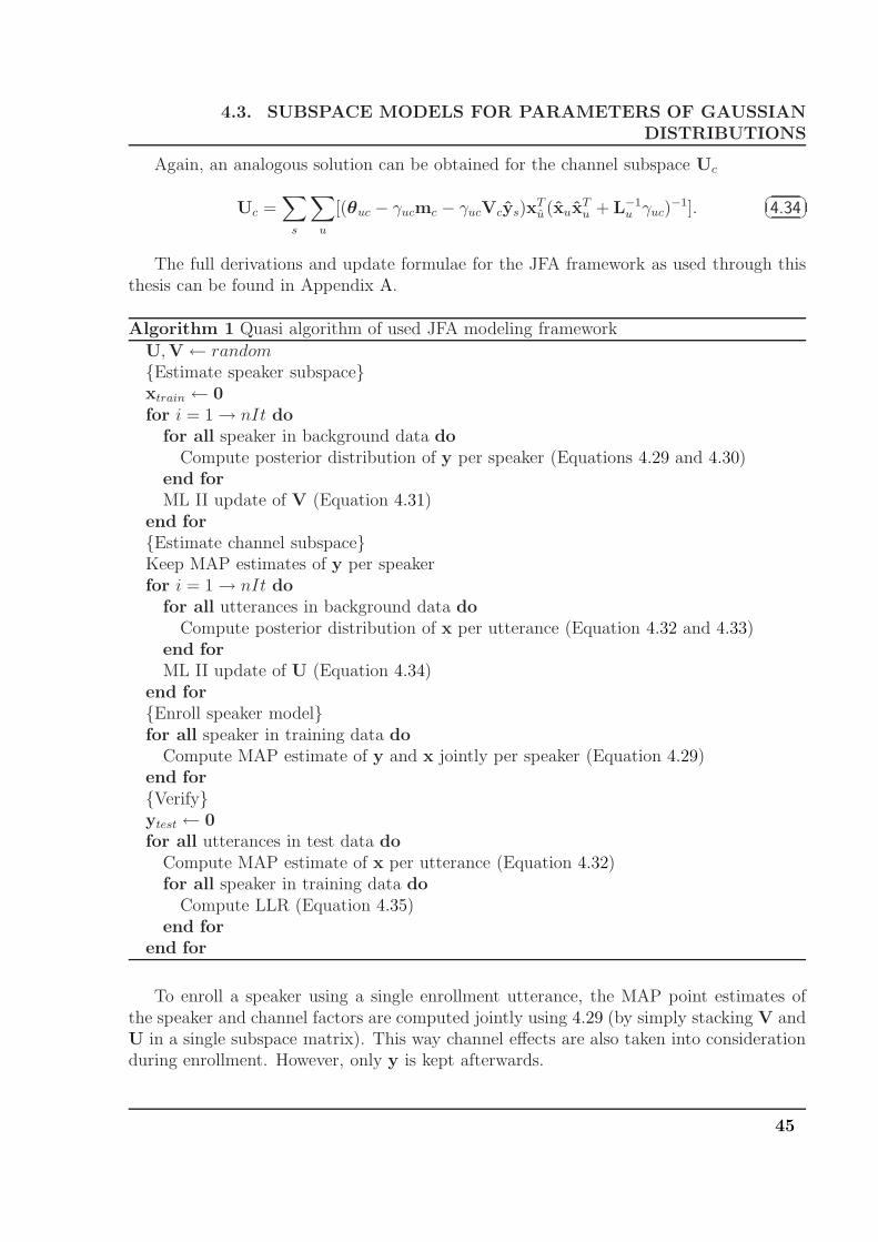
4.3. SUBSPACE MODELS FOR PARAMETERS OF GAUSSIANDISTRIBUTIONS
Again, an analogous solution can be obtained for the channel subspace Uc
Uc =∑
s
∑
u
[(θuc − γucmc − γucVcys)xTu (xux
Tu + L−1
u γuc)−1].
��
��4.34
The full derivations and update formulae for the JFA framework as used through thisthesis can be found in Appendix A.
Algorithm 1 Quasi algorithm of used JFA modeling framework
U,V← random{Estimate speaker subspace}xtrain ← 0for i = 1→ nIt do
for all speaker in background data doCompute posterior distribution of y per speaker (Equations 4.29 and 4.30)
end forML II update of V (Equation 4.31)
end for{Estimate channel subspace}Keep MAP estimates of y per speakerfor i = 1→ nIt do
for all utterances in background data doCompute posterior distribution of x per utterance (Equation 4.32 and 4.33)
end forML II update of U (Equation 4.34)
end for{Enroll speaker model}for all speaker in training data do
Compute MAP estimate of y and x jointly per speaker (Equation 4.29)end for{Verify}ytest ← 0for all utterances in test data do
Compute MAP estimate of x per utterance (Equation 4.32)for all speaker in training data do
Compute LLR (Equation 4.35)end for
end for
To enroll a speaker using a single enrollment utterance, the MAP point estimates ofthe speaker and channel factors are computed jointly using 4.29 (by simply stacking V andU in a single subspace matrix). This way channel effects are also taken into considerationduring enrollment. However, only y is kept afterwards.
45

CHAPTER 4. MODELING APPROACHES FOR PROSODIC SPEAKERVERIFICATION
By using solely point estimates in the enrollment and verification process, the speaker-and channel adapted mean supervector can be constructed using the JFA model for eachenrollment-speaker – test-utterance combination. Here, we make another assumption:
• The channel factors during verification are solely estimated using the UBM (y set to0). This way, the channel has to be estimated only once per test utterance, insteadof estimating it for each test-utterance/model combination in test.
Experiments indicated that this simplification does not harm the performance but greatlyreduces the computational load.
Then, the same frame-by-frame Log Likelihood Ratio (LLR) computation (Equation4.19) can be used for scoring as for the standard approaches without subspace mod-eling. However, more efficient approaches have been proposed and were compared by[Glembek et al., 2009].
The so-called fast scoring technique for JFA has proven to be much more computa-tionally efficient than the standard likelihood evaluation. Fast scoring for JFA is based onfurther approximations:
• The assignment of feature frames to Gaussian components is solely based on theUBM. The scoring technique uses the same sufficient statistics as are used in UBM orJFA parameter re-estimation (Equations 4.2 and 4.3). This way, the GMM evaluationof each feature frame is only needed once, using the UBM, and further processingsteps are only based on the fixed-sized statistic vectors.
• As the statistics based on the UBM are used, the true likelihood of the data given themodel is approximated by the same auxiliary function as used in an EM algorithm(see also Section A.1).
• The quadratic auxiliary function is further simplified by a linear approximation usingfirst-order Taylor series.
This reduces the computational demand to a simple dot-product scoring of channelcompensated statistic supervectors leading to the following scoring function:
LLRfast =∑
c
yTs VT
c Σ−1c (θc − γcmc − γcUcx).
��
��4.35
The whole process of hyperparameter estimation, training and test is sketched in thequasi algorithm 1. A tutorial-style implementation of the described JFA framework canbe found at [Glembek, 2009]. This framework dominated the 2008 NIST SREs and wasbroadly adopted during the NIST SRE 2010.
4.3.2 Total variability subspace
Besides the great success of the JFA model, it was found during the JHU Summer Workshopon Robust Speaker Recognition [Burget et al., 2008], that even the channel-related latentvariables x still contain information to discriminate between speakers.
46

4.3. SUBSPACE MODELS FOR PARAMETERS OF GAUSSIANDISTRIBUTIONS
Based on these findings, [Dehak et al., 2009b] proposed a simplified variant of the JFAframework, that assumes that speaker and channel subspaces are not independent and usesonly one subspace covering the total variability in an utterance:
φGaussIV = m + Tw.��
��4.36
Again, T spans a low-dimensional linear subspace in the original mean parameter space.Also, the subspace size RT is much smaller than D × C, usually around 400. The com-ponents of w are the low-dimensional latent variables corresponding to coordinates in thetotal variability subspace.
The key idea of the total variability modeling is to learn a single low-dimensionalsubspace T in which the model parameters live. The model can then be used to extractlow-dimensional representations of each utterance (the latent factors w), by adapting themodel to each utterance. This way, the features per utterance are reduced to a single vectorwith a few hundred dimensions, while keeping most of the important information. Thismakes it possible to apply various machine learning techniques for the final verification,which were not applicable to high-dimensional sequential data.
The simplified JFA model is again a probabilistic model, where the latent variables ware distributed according to a standard normal prior:
p(w) = N (w|0, I).��
��4.37
This again leads to a closed-form solution of the posterior distribution of the latent variable:
p(w|ou) = N (wu|wu,L−1u ).
��
��4.38
The re-estimation of the model parameters is based on the same EM algorithm as usedin the previous section. For the total variability factors w, the mean of the posteriordistribution is given as:
wTu =
∑
c
(θTuc − γucm
Tc )Σ−1
uc TcL−1u ,
��
��4.39
where Tc is the D×RT block of T corresponding to the cth component, with the precisionmatrix of the posterior distribution
Lu =∑
c
γucTTc Σ−1
c Tc + IT��
��4.40
and IT being an RT × RT identity matrix. Analogously to the JFA framework, keepingthe distribution of the latent variables for each utterance fixed, it is in turn possible toreestimate the subspace matrix T:
Submatrix Tc corresponding to cth block of T can be re-estimated as
Tc =∑
u
[(θuc − γucmc)wTu (wuw
Tu + L−1
u γuc)−1].
��
��4.41
47

CHAPTER 4. MODELING APPROACHES FOR PROSODIC SPEAKERVERIFICATION
Note, that this time no speaker labels are used at all and the latent vector distributionsare computed for each utterance in the training data.
In this approach, the JFA-like model serves only as the extractor of the vectors w,which can be seen as low-dimensional fixed-sized representations of utterances, and whichare in turn used as inputs to another classifier. The low-dimensional vector w is also knownas an iVector.
Note, that unlike the standard JFA, where two subspaces are used to account for speakerand intersession variability, the iVector variant uses a single subspace accounting for allthe variability. Therefore, the extracted vectors w are not free of channel effects, andintersession compensation must be eventually considered during classification.
[Dehak et al., 2009b] originally proposed to classify the iVectors using SVMs. Due tothe low-dimensionality (usually in the order of hundreds), intersession variability compen-sation could be efficiently incorporated into the SVM kernel. Eventually, a simple cosinedistance scoring approach that is solely measuring the angle between two iVectors resultedin the most efficient method:
scorecosine =〈w1,w2〉‖w1‖‖w2‖
.��
��4.42
For evaluating trials, its should be mentioned that using the iVector model completelysymmetrizes the problem: It does not matter anymore which utterance in a trial is thetraining, and which is the test utterance. The task is simply to compare the two iVectors.
Normalization techniques, like zt-norm can be included very efficiently, by simply“adding” iVectors for each t-norm utterance to the training iVectors and “adding” iVectorsfor each z-norm utterance to our test iVectors. This way, the Gram matrix containing allcosine-distance scores already includes all scores needed to compute the zt-norm statistics.
Intersession compensation was incorporated in the iVector feature domain by standardLinear Discriminant Analysis (LDA) followed by Within-Class Covariance Normalization(WCCN) [Hatch et al., 2006]. First, the within-class and the between-class covariancematrices need to be trained on iVectors estimated on a large hold-out set. Usually, thesame background set as used for the UBM or the iVector training. The between class B iscomputed as
B =S∑
s=1
Ns(ws −w)(ws −w)T��
��4.43
with ws = 1Us
∑Us
u wu being the mean of the iVectors per speaker and w = 1U
∑Uu wu being
the mean of all iVectors in the data set. Ns is the number of iVectors per speaker s. Thewithin class W is computed as
W =
S∑
s=1
Us∑
u
(wu −ws)(wu −ws)T .
��
��4.44
The LDA matrix A consists of the eigenvectors of
W−1B.��
��4.45
48

4.3. SUBSPACE MODELS FOR PARAMETERS OF GAUSSIANDISTRIBUTIONS
Figure 4.1: LDA assumption in iVector space.
Usually A is sorted according to the corresponding eigenvalues. This way, meaningfuldimensionality reduction can be performed by keeping simply the n leading basis.
With a LDA matrix A computed using iVectors from a background set and the speakerlabels, each iVector w can be transformed first by the LDA. Next, the WCCN matrix W−1
is trained to whiten the within-class covariance matrix of the LDA transformed featurespace. It is estimated using 4.44 on the transformed iVectors. Incorporating both into thecosine scoring, equation 4.42 can be rewritten as:
scoreLDA+WCCN =wT
1 AW−1ATw2√
wT1 AW−1ATw1
√
wT2 AW−1ATw2
.��
��4.46
As this is not a likelihood-ratio, normalization is needed, usually zt-norm.
However, this approach has been significantly outperformed by the use of a ProbabilisticLinear Discriminant Model (PLDA) [Prince, 2007] to model speaker and session variabilityin iVector space. As this model will mainly be used for the iVector based experiments, itis explained in more detail in the following section.
49

CHAPTER 4. MODELING APPROACHES FOR PROSODIC SPEAKERVERIFICATION
4.3.3 Probabilistic Linear Discriminant Analysis
The fixed-length iVectors extracted per utterance can be used as input to a pattern recog-nition algorithm. Here, a probabilistic framework is used, where speaker and intersessionvariability in the iVector space is modeled using across-class and within-class covariancematrices Σac and Σwc. It is assumed that latent vectors s representing speakers are dis-tributed according to
p(s) = N (s|m,Σac)��
��4.47
and for a given speaker s, the iVectors are distributed as
p(w|s) = N (w|s,Σwc).��
��4.48
Figure 4.1 exemplifies this assumption by a toy example in 2D iVector space. Thedots represent several iVectors extracted from several utterances corresponding to fourdifferent speakers. It can be observed, that the four solid dots, representing the explicitspeakers means s, are Gaussian distributed with mean m and covariance Σac. Further,the individual iVectors per speaker are also Gaussian distributed with its mean s and aglobally tied covariance Σwc. Using this model, it becomes clear that two new data points(red squares) are likely to belong to the same speaker although they are quite far apartfrom each other. As it is a probabilistic model, we can compute likelihoods of data andthe parameters m, Σac and Σwc can be estimated using ML (EM algorithm).
Further, in the Probabilistic Linear Discriminant Analysis Model (PLDA) [Prince, 2007],it is assumed that the speaker and/or intersession variability can be modeled using sub-spaces. PLDA can be seen as a special case of JFA ([Kenny et al., 2008b], Section 4.3.1)with a single Gaussian component. Here, a simplified variant (SPLDA) is used, which weadapted from [Brummer, 2010]. The across-class covariance matrix is modeled using a sub-space as Σac = VTV, which limits the speaker variability to live in a subspace spanned bythe columns of the reduced rank matrix V. With full-rank within-class covariance matrixΣwc = D−1, the distribution of the iVectors w can be rewritten as:
w = m + Vy + �
��4.49
incorporating a low-dimensional speaker subspace V and ε being a noise variable (coveringthe channel effects) with precision matrix D.
Similar to the JFA model, the latent variables y are distributed according to a zero-mean unit-covariance Gaussian prior:
p(y) = N (y|0, I), p(ε) = N (ε|0,D−1).��
��4.50
ML and minimum divergence update of parameters
Now, a simplified version of an EM algorithm [Brummer, 2010] with minimum divergenceupdate is presented, to estimate the SPLDA model parameters.
50

4.3. SUBSPACE MODELS FOR PARAMETERS OF GAUSSIANDISTRIBUTIONS
The global mean parameter m is simply defined by the mean of all iVectors wsu in thetraining data, with s = 1 . . . S speakers and u = 1 . . . Us observations per speaker s. Thezero order statistics per speaker are simply Us and the first order statistics are defined as:
fs =Us∑
u=1
wsu −m.��
��4.51
The global second order statistic is:
S =
SU∑
u=1
(wsu −m)(wsu −m)T .��
��4.52
The posterior of the speaker factors given all the observations Ws = [ws1 . . .wsus] is
normally distributed with:p(ys|Ws) = N (ys|ys,P
−1),��
��4.53
where the precision matrix of the posterior is
Ps = Us(VTDV) + I
��
��4.54
and the mean of the posterior distribution is given as
ys = P−1s VTDfs.
��
��4.55
Two helper variables Q and R are introduced that are accumulated over all speakers:
Q =∑
s
ysfTs ,
��
��4.56
R =∑
s
Us(P−1 + ysy
Ts ).
��
��4.57
Further, for the minimum divergence update
Y =1
S
S∑
s=1
(P−1 + ysyTs )
��
��4.58
is accumulated.Using the complete-data likelihood function for speaker s
p(Ws|ys,V,D) =Us∏
u=1
N (wsu|Vys,D−1)
∝ exp
Us∑
u=1
(−1
2wT
suDwsu + wTsuDVys −
1
2yT
s VTDVys),��
��4.59
51

CHAPTER 4. MODELING APPROACHES FOR PROSODIC SPEAKERVERIFICATION
we can obtain the EM auxiliary function to maximize
〈∑
s
log p(Ws|ys,V,D) + const〉
=N
2log |D| − 1
2tr(SD)− 1
2tr(RVTDV) + tr(QDV).
��
��4.60
The maximum likelihood update for V is then given by:
V = R−1Q��
��4.61
and D−1 can be updated as
D−1 =1
N(S−VQ)
��
��4.62
with N being the global zero order statistics∑S
s=1 Us. Finally, minimum divergence re-estimation of V gives:
V← Vchol(Y)T��
��4.63
where chol(Y)chol(Y)T = Y denotes the Cholesky decomposition. This scheme is usedin an iterative manner that usually converges in less than ten iterations.
Score evaluation for a pair of iVectors
After parameter estimation, the SPLDA model can be directly used to evaluate speakertrials incorporating two iVectors w1 and w2 due to its probabilistic nature. Following thework of [Burget et al., 2011] the needed formulae are provided below. For a more generalview, allowing multiple enrollment iVectors, see [Brummer and de Villiers, 2010].
Using the trained SPLDA model and Equations 4.47 and 4.48, one can directly evaluatethe log-likelihood ratio between two hypotheses:
1. Hs: Both iVectors were generated from (a mode of) a single speaker.
2. Hd: The two iVectors were generated independently (from two different speakers).
The LLR is computed as:
LLRPLDA = logp(w1,w2|Hs)
p(w1,w2|Hd)= log
∫p(w1|s)p(w2|s)p(s)ds
p(w1)p(w2).
��
��4.64
The numerator gives the marginal likelihood of producing both iVectors from the samespeaker, while the denominator is the product of the marginal likelihoods that both iVectorsare produced independently. The integrals can be evaluated analytically and scoring canbe performed very efficiently:
LLRPLDA = wT1 Λw2 + wT
2 Λw1 + wT1 Γw1 + wT
2 Γw2 + (w1 + w2)Tc + k
��
��4.65
52

4.3. SUBSPACE MODELS FOR PARAMETERS OF GAUSSIANDISTRIBUTIONS
with
Γ = −1
4(Σwc + 2Σac)
−1 − 1
4Σ−1
wc +1
2Σ−1
tot ,��
��4.66
Λ = −1
4(Σwc + 2Σac)
−1 +1
4Σ−1
wc ,��
��4.67
c = ((Σwc + 2Σac)−1 −Σ−1
tot)m,��
��4.68
k = log |Σtot| −1
2log |Σwc + 2Σac| −
1
2log |Σwc|+ mT (Σ−1
tot − (Σwc + 2Σac)−1)m,
��
��4.69
and the total covariance matrix given by
Σtot = Σac + Σwc = VTV + D−1��
��4.70
with Σwc = D−1 (see 4.62) and Σac = VTV (see 4.63).
4.3.4 Experiments
Both techniques, the JFA as well as the iVector modeling, are applicable to the low-dimensional well-defined DCT features as presented in Section 3.
The initial baseline system was a standard UBM-GMM system with MAP adaptation[Reynolds et al., 2000]. In Section 3.1.5, results for this basic system, using the simpleDCT contour features were presented. An EER of around 25% on the 2006 NIST SREtask was obtained.
Joint Factor Analysis for DCT contour features
Prior to the NIST Speaker Recognition Evaluations 2008, the JFA approach as described inSection 4.3.1 could be applied to the same prosodic contour features leading to significantimprovements [Kockmann and Burget, 2008b].
First, we will describe how the JFA model is trained. The starting point is again aUBM. We train two gender dependent models with 256 Gaussian components each anddiagonal covariances, using the background data set (see Section 2.2.1). Further, for eachutterance in the background set, zero and first order sufficient statistics are collected usingthe final UBM.
Then, the JFA model itself can be trained as described in Algorithm 1. The meanvector m is set to the concatenated UBM means. The used mean supervector dimensionis 256 × 13 = 3328 and the speaker-subspace size is chosen as RV = 50 and the channel-subspace size RU = 20, similar to the setup in [Dehak et al., 2007]. Both matrices U andV are randomly initialized and are retrained in 10 iterations. Note, that only speakers,that have at least five sessions in the background data set are used.
Following Algorithm 1, with all JFA hyperparameters fixed, the speaker models can betrained and evaluated. Again, the 2006 NIST SRE core condition is used, and for eachtraining utterance, speaker- and channel factors y and x are estimated jointly by stackingU and V into a single 70-dimensional subspace.
53

CHAPTER 4. MODELING APPROACHES FOR PROSODIC SPEAKERVERIFICATION
Norm Male Female Both
none 18.23 16.27 17.12
z-norm 18.48 15.64 16.47
t-norm 15.83 13.90 14.73
zt-norm 15.69 13.35 14.37
(a) Standard LLR
Norm Male Female Both
none 15.96 14.17 15.00
z-norm 16.22 15.45 15.28
t-norm 14.08 11.53 12.40
zt-norm 14.63 13.07 12.95
(b) Fast scoring
Table 4.1: DCT contour features with pseudo-syllable segmentation modeled by JFA withtwo different scoring techniques. Results in EER [%] for SRE 2006 core condition.
Finally, channel factors x are estimated for each test utterance in the NIST SRE 2006data set. As mentioned earlier, we estimate the channel factors for the test utterancesbased on the UBM only by setting y to zero.
The first line in Table 4.1.a shows great improvements achieved due to the JFA modelingwith conventional LLR scoring. While around 25% EER is obtained with the standardGMM-UBM approach, the EER can be significantly reduced to 17%.
Next, also score normalization techniques as described in [Auckenthaler et al., 2000]are applied. For this purpose, several hundred z- and t-norm utterances are randomlytaken from the background data set. While z-norm already improved the performance,a great improvement is obtained by using t- or even zt-norm (meaning first to apply z-and then t-norm). While z-norm parameters can be pre-computed, especially t-norm iscomputationally expensive, as several hundred extra trials per test utterance have to beevaluated to obtain the normalization statistics.
The fast-scoring technique that reduces the likelihood evaluation to a dot-product scor-ing has already been introduced in Section 4.3.1. Especially for the evaluation of a bigt-norm cohort (each t-norm speaker has to be scored against each test utterance), thistechnique seems to be very appropriate. As the results in Table 4.1.b indicate, the tech-nique is not only much faster, but seems to be even more robust and results in significantlybetter performance. It is also interesting to see, that both prosodic JFA systems workreasonably well without any normalization, which is usually not the case using low-levelcepstral features.
Beside these results, many more experiments were conducted during the work on thisthesis, mainly investigating into:
• Optimal subspace sizes: Different from cepstral systems, the optimal number ofeigenvoices RVwas found to be 50–100 and the number of eigenchannels RU 20–40.
• Optimal model sizes: Depending on the amount of training data, the optimal numberof Gaussian components C was 256–1024.
54

4.3. SUBSPACE MODELS FOR PARAMETERS OF GAUSSIANDISTRIBUTIONS
• Amount of training data: While increasing the amount of data for the UBM doesnot improve the performance much, a rule of thumb for the JFA model can be: “Themore, the better”.
• JFA training style: Joint estimation of U and V [Kenny et al., 2005] or iterativere-estimation (also taking channel into account when estimating the speaker matrix)did not improve the performance.
• Minimum-divergence training: As proposed by [Kenny et al., 2008b], did not im-prove the performance but achieves a faster convergence and requires less trainingiterations.
• Scoring with integration over the channel distribution: A technique used in the origi-nal JFA system proposed by [Kenny et al., 2005] performs equally to the fast-scoringtechnique, but is much slower.
iVector modeling for DCT contour features
During NIST SRE 2010 system development [Brummer et al., 2010], we tried to apply theiVector approach as described in Section 4.3.2 to the DCT contour features, as it greatlyoutperformed the standard JFA approach on cepstral systems [Dehak et al., 2009a].
Both models, JFA and iVector models, were trained and compared. For both, thestaring points are gender dependent UBMs trained on the background data. As the NISTSRE 2008 data set was used for development (see Section 2.2.3), the NIST 2006 dataset was included into the background data set. Due to the larger amount of data, largermodels with 1024 Gaussian components were used. Again, sufficient statistics are collectedfor each utterance in the background set, which are used for training the JFA as well asfor training the iVector extractor.
The JFA model was trained exactly as described in the previous section with 100eigenvoices and 40 eigenchannels per gender. The total variability model is trained in asimilar manner. The total variability matrix T with a size RT = 100 is randomly initializedand is trained in 10 iterations of the algorithm as described in Section 4.3.2.
Then, the iVector model parameters are fixed and the model can be used as a front-end to collect iVectors for all training and test utterances. This is first done for eachutterance in the background set. Based on these iVectors, a deterministic LDA+WCCNchannel compensation scheme as described in Section 4.3.2 was computed. Using thespeaker labels, within class and across class covariance matrices are computed based onthe iVectors to obtain a LDA transformation, reducing the dimensionality of the iVectorsto 75. Based on the transformed 75-dimensional iVectors, a full-rank WCCN matrix iscomputed and applied.
When comparing the results on EER in Table 4.2, very disappointing results for theiVector approach with syllable based segmentation and cosine distance scoring are obtained.This iVector configuration achieves results that are about 40% relative worse than thestandard JFA model.
55

CHAPTER 4. MODELING APPROACHES FOR PROSODIC SPEAKERVERIFICATION
Model Segmentation Scoring EER
JFA Syllable Fast scoring 11.97iVector Syllable LDA 75 + WCCN + Cosine distance 16.86
JFA Fixed Fast scoring 9.36iVector Fixed LDA 75 + WCCN + Cosine distance 12.12iVector Fixed PLDA 100 8.42
Table 4.2: JFA vs. iVector modeling for different DCT contour feature segmentations andscoring methods on SRE 2008 telephone condition. All with zt-norm, except the PLDAmodel.
However, in recent experiments [Kockmann et al., 2011c] we have shown that the iVec-tor modeling itself is superior to the JFA approach. Mainly two things changed comparedto the above experiments. First, the fixed window size segmentation as proposed in Section3.1.2 was used with a window size of 300ms and a frame-shift of only 50ms. It was found,that while already good results were obtained compared to the pseudo-syllable segmen-tation (see results in Section 3.1.5), reducing the frame-shift from 150ms to 50ms greatlyimproved the performance.
For a comparable JFA system as used in the last experiments, this already improved thegeneral system performance, as can be seen in the third row of Table 4.2, leading to an EERof under 10% on the NIST 2008 tel-phn:tel-phn condition. Note, that many more framesare extracted using this segmentation technique due to the high overlap of consecutivewindows. This seems to be generally helpful for the system performance. However, we didnot systematically optimize the frame-shift size.
Using these features for an iVector model with LDA+WCCN as in the latter exper-iments, still resulted in worse results for iVector approach, but decreased the EER from16% to 12%. New was to apply the PLDA model for trial evaluation, as described inSection 4.3.3. We used a full-rank 100-dimensional speaker subspace V and no furthernormalization. This greatly improved the performance resulting in an EER of 8.4%, 10%relative better than the JFA system. Note, that score normalization techniques were notfound to be helpful for the PLDA model. The best scores were always obtained withoutany score normalization, indicating that the scores are already well distributed due to theprobabilistic nature and evaluation of the LLR scores.
4.4 Subspace models for parameters of multinomial
distributions
As described in the last section, there were successful attempts to apply JFA and recentlyalso iVector modeling to prosodic features. However, only a small subset of well-definedcontinuous prosodic features, as the proposed DCT contour features, can be used with JFA.
56

4.4. SUBSPACE MODELS FOR PARAMETERS OF MULTINOMIALDISTRIBUTIONS
In [Ferrer et al., 2010], the two most popular prosodic speaker verification approaches arecompared:
1. JFA modeling of a subset of prosodic contour features.
2. Discretizing (binning) a full set of SNERF prosodic features, representing it as avector of soft counts and modeling it using SVM.
Further, the two modeling techniques are compared using exactly the same subset of con-tour features, once modeling the features directly using JFA and once converting the fea-tures to soft counts and modeling them using SVMs. Although JFA compares favorablyto SVM on the subset of well-defined continuous contour features, a significant gain canbe obtained with SVMs trained on count super-vectors based on SNERFs (see Section 3.2)when prosodic features – that JFA cannot deal with – are added.
In this section, an approach is proposed to combine the advantage of the JFA-likesubspace model with the flexibility of representing highly complex heterogeneous prosodicSNERF features.
A similar idea of subspace modeling of multinomial distribution was proposed for inter-session variability compensation in phonotactic language identification [Glembek et al., 2008].A related model is also applied for modeling GMM weights in Subspace GMM (SGMM),which is a recently proposed acoustic model for speech recognition [Povey and Burget, 2011].
4.4.1 Total variability subspace
Based on the success of the iVector approach for cepstral features, there was a motivationto develop the simplified JFA-like variant with only a single total variability subspace forSNERFs. As described in Section 3.2, the SNERFs are parameterized to discrete classcounts based on GMMs.
As a generative model, a multinomial distribution appears as a natural choice for model-ing the counts resulting from this step. More precisely, a set of E multinomial distributionsis required, one for each GMM in the ensemble. Each multinomial distribution correspondsto a set of Ce probabilities, one probability φec for each Gaussian c in the GMM e. For eachframe, each GMM is expected to generate a feature by one of its components with proba-bility given by the multinomial distribution. This corresponds to co-occurring events thatshould be modeled by separate multinomial distributions (as all SNERF feature-tokensare modeled independently of each other). Each multinomial distribution lives in a n-dimensional simplex and the space of all parameters is the Cartesian product of all thesimplexes for all the separate distributions. The bottom row of Figure 4.2 illustrates thisfor the toy example already used when SNERFs were introduced in Section 3.2. Remem-ber, three prosodic measurements are extracted (first row) and parameterized by individualsmall GMMs (second row). Now, as each mixture component represents a discrete class,a multinomial distribution is obtained for each prosodic feature. The parameters of theduration model exist on a line; the pitch model parameters, in a 2D simplex; and theenergy parameters, in a 3D simplex space.
57

CHAPTER 4. MODELING APPROACHES FOR PROSODIC SPEAKERVERIFICATION
0 50 100 150 200 250 3000
50
100
150
200
250
300
Fre
quen
cy [H
z]
0 50 100 150 200 250 30020
30
40
50
60
70
80
Ene
rgy
−20 0 20 40 60 800
0.01
0.02
0.03
0.04Duration: 2 mixtures
3 3.5 4 4.5 5 5.5 6 6.50
0.2
0.4
0.6
0.8
1Pitch: 3 mixtures
0 0.5 10
0.5
1
1.5
2
2.5Energy: 4 mixtures
Duration: 2 classes Pitch: 3 classes Energy: 4 classes
and uh where are you where which state are you
6.3
3.7
0.3
1.2
8.5
2.1
1.9 2.73.3
1
2
3 4
5
6
7
8
9
Figure 4.2: Top row: Extraction of three SNERF parameters from a speech segmentcontaining 10 single-syllable words: Syllable duration (determined by black vertical lines),mean pitch value per syllable (blue squares), and mean energy per syllable (red stars).Middle row: Parameterization of SNERF sequences: Small GMMs are trained on back-ground data for each individual SNERF. Two mixtures are used for duration, three mix-tures for pitch, and four mixtures for energy. Occupation counts for the values extractedin the top row (here as bars) are collected using the GMMs. Bottom row: Multino-mial model spaces for duration, pitch, and energy. The colored lines show various one-dimensional iVectors (the values are mapped to colors) projected to the full ensemble ofmultinomial spaces.
In the proposed Subspace Multinomial Model (SMM), it is assumed that the multino-mial distributions differ from utterance to utterance. In the case of SNERFs, parametersof many multinomial distributions need to be estimated. Therefore, a way to estimateall the parameters robustly given a limited amount of data available for each utterance isdesired. It is assumed that there is a low-dimensional subspace of the parameter space inwhich the parameters for individual utterances live.
For this reason, an explicit latent variable w is introduced through which the probabilityof cth class of multinomial distribution e in the ensemble is:
φec =exp(mec + tecw)
∑Ce
i=1 exp(mei + teiw),
��
��4.71
with tec being the cth row of eth block of a low-dimensional subspace matrix T (size∑E
e=1 Ce×RT), which spans a linear subspace that is generally non-linear in the simplex ofclass probabilities due to the softmax function. Figure 4.2 shows how the subspace restrictsthe movement in the simplex in a non-linear way (colored lines). By drawing values for
58

4.4. SUBSPACE MODELS FOR PARAMETERS OF MULTINOMIALDISTRIBUTIONS
a one-dimensional variable w from minus infinity to infinity, the model moves in all threesimplexes simultaneously along the non-linear, single-dimensional manifolds.
Now, all the multinomial distributions corresponding to one utterance can be repre-sented by a single low-dimensional vector w. This way, (1) the number of free parametersto efficiently model differences between individual utterances can be reduced, and (2) de-pendencies between the individual SNERFs can be learned.
The model parameters are estimated by iteratively re-estimating the latent variables wfor each utterance in the training data to maximize the likelihood function based on thecurrent estimate of T, and vice-versa.
Using the final estimate of T, w vectors (which are also called iVectors) can be extractedfor new data. This way, the model is used as a feature extractor and each iVector can beseen as a low-dimensional representation of the whole utterance.
Next, re-estimation formulae for the proposed subspace model are presented. For sim-plicity, a single multinomial distribution is used and we show how to extend the frameworkto the general case with arbitrary number of multinomial distributions. While only the finalupdate formulae needed for implementation are given in this section, the whole derivationcan be found in Appendix B.
Likelihood function
The log-likelihood of data O for a multinomial model with C discrete classes is determinedby the vector of model parameters φ and vector of sufficient statistics γ, representing theoccupation counts of classes for all U utterances in O:
log p(O) =U∑
u=1
C∑
c=1
γuc log φuc,��
��4.72
where γuc is the occupation count for class c and utterance u and φuc are the probabilities ofthe (utterance dependent) multinomial distribution, which is defined by a subspace modelaccording to Equation 4.71:
φuc =exp(mc + tcwu)
∑Ci=1 exp(mi + tiwu)
,��
��4.73
where mc is a speaker independent mean parameter, tc is the c-th row of subspace matrixT and wu is an RT-dimensional column vector (iVector) representing speaker and channelof utterance u.
Parameter re-estimation
The model parameters are obtained by maximum likelihood (ML) estimation. First, thesubspace parameters m and T need to be estimated from training data. This is an it-erative process, alternating between estimating subspace parameters m and T with fixediVectors, and estimating iVectors wu (one for each training utterance) with fixed subspace
59

CHAPTER 4. MODELING APPROACHES FOR PROSODIC SPEAKERVERIFICATION
parameters. Even with fixed subspace parameters, there is no closed-form solution for theML update of iVectors, and each iVector must be updated using an nonlinear optimizationtechnique, which is again an iterative procedure. Likewise, there is no closed-form solutionfor the ML update of the subspace parameters with fixed iVectors.
An efficient iterative optimization scheme based on Newton methods [Fletcher, 2000]can be applied which uses a local quadratic approximation to the log likelihood function.In Appendix B, the full derivations for a Newton-Raphson update scheme based on thelog-likelihood function 4.72 are given.
However, the final updates adopted in our implementation are based on updates derivedfor Subspace GMMs [Povey and Burget, 2011]. These differ mainly in the way that anapproximate Hessian is used, and lead to better convergence. Another alternative wouldbe to use quasi Newton methods [Jorge and Stephen, 2006, Chapter 6] like the BFGSalgorithm, that do not need to evaluate the Hessian matrix explicitly.
In the used implementation, vectors wu are updated as
wnewu = wold
u + H−1u gu,
��
��4.74
where gu is the gradient of the log likelihood function
gu =C∑
i=1
tTi (γui − φold
ui
C∑
j=1
γuj)��
��4.75
and Hu is an RT × RT matrix
Hu =
C∑
i=1
tTi ti max(γui, φold
ui
C∑
j=1
γuj),��
��4.76
where φoldui refers to the multinomial distribution (4.73) defined by the parameters from the
preceding iteration. Note that the matrix Hu can be interpreted as an approximation tothe Hessian matrix and the update formula (4.74) can be then seen as a Newton-Raphsonupdate. The rows of matrix T are updated as
tnewc = told
c + H−1c gc,
��
��4.77
where gc is the gradient of the log likelihood function
gc =U∑
u=1
(γuc − φolduc
C∑
i=1
γui)wTu
��
��4.78
and Hc is an RT ×RT matrix
Hc =
U∑
u=1
max(γuc, φolduc
C∑
i=1
γui)wuwTu .
��
��4.79
60

4.4. SUBSPACE MODELS FOR PARAMETERS OF MULTINOMIALDISTRIBUTIONS
The updates for both wu and T may fail to improve the likelihood by making too largean update step. In the case of such failure, the update step is halved until an increase inlikelihood is obtained.
Vector m is usually set to the logarithm of the normalized counts of the whole back-ground data set and kept fix during re-estimation and is not updated. However, retrainingm can be simulated by fixing one of the coefficients in vectors wu to be one and setting thecorresponding column of matrix T as the vector m. However, We never saw any benefitfrom further retraining m.
Algorithm 2 Quasi-algorithm for SMM training and prosodic iVector extraction.
{Estimate total variability subspace}m← log of mean of background data probabilitiesT← PCA of 4.80 (or random)w← 0for i = 1→ number of outer iterations do
for j = 1→ number of inner w iterations dofor all utterances in background data do
Update w per utterance (4.74)end for
end forfor k = 1→ number of inner T iterations do
for all rows in T doUpdate t (4.77)
end forend for
end for{Estimate iVectors}w← 0for j = 1→ number of inner w iterations do
for all utterances in background/enrollment/test data doUpdate w per utterance (4.74)
end forend for
So far, only subspace modeling of single multinomial distribution is considered in theequations. However, for the prosodic features extracted by the ensemble of GMMs, theoccupation counts should be modeled by a set of multinomial models, one for each GMM.These are considered to be concatenated into a single super-vector of multinomial distri-butions, which is modeled by one subspace matrix T. In other words, there will be onlyone iVector wu defining the whole set of multinomial distributions for each utterance u.To achieve this, the indices c from Equation (4.73) must be divided into subsets, whereeach subset corresponds to mutually exclusive events (counts from one GMM). Then, theonly difference will be in the denominator of (4.73), where the normalization will be per-
61

CHAPTER 4. MODELING APPROACHES FOR PROSODIC SPEAKERVERIFICATION
formed only over the appropriate subset of indices that the current c belongs to (just likein Equation 4.71).
After the subspace parameters are estimated on training data, the model can be usedto extract iVectors wu for all enrollment, test and background utterances using the sameupdate formulae (4.74–4.76). The whole training process is exemplified in Algorithm 2.
Model initialization
While Section 4.4.1 contains a quite general description of the training procedures, themodel initialization is described here more specifically for the used system. First, themultinomial distributions for individual GMMs from the ensemble are estimated using alltraining utterances. This corresponds to summing all training super-vectors of occupationcounts and normalizing the resulting super-vector over the ranges corresponding to theindividual GMMs. Such super-vector of multinomial distributions (holding the individualclass probabilities) is denoted as svUBM . The vector m is simply initialized to a logof svUBM . Note, that no advantage from its further retraining was observed using theupdates from the previous section. All vectors w are initialized to zeros. To ensure a goodstarting point, the subspace matrix T is initialized to the eigenvectors of the covariancematrix computed from smoothed utterance super-vectors svu centered around the vectorm, where coefficient c of vector svu is defined as:
svuc = log(αγuc
fuc+ (1− α)svUBMuc
),��
��4.80
where fuc is the number of feature frames seen for the utterance and for the GMM thatthe occupation count γuc corresponds to. The smoothing constant α = 0.9 ensures thatthe log of zero is not taken for classes that have not been occupied at all by any frames ofutterance u.
4.4.2 Experiments
Training algorithm
First experiments are performed to evaluate the convergence properties of three possibleways to train the subspace model:
1. Gradient Descent (GD): Subspace and iVectors are solely updated using the gradientof the error function with a fixed learning rate parameter η: In Equations 4.74 and4.77, the Hessian term is substituted with a fixed parameter η.
2. Newton-Raphson, Iterative Reweighted Least Squares (IRLS): A full IRLS update isused for subspace and iVectors as described in Appendix B. Note, that the evaluationof the full Hessian matrix is needed, which is infeasible for large subspaces.
3. Hessian approximation (HA): This approximation of the Hessian is adopted from[Povey and Burget, 2011] (Equations 4.74–4.79). It is claimed that this leads tobetter convergence properties than the full IRLS.
62

4.4. SUBSPACE MODELS FOR PARAMETERS OF MULTINOMIALDISTRIBUTIONS
0 2 4 6 8 10 12 14 16 18 20−6.9
−6.85
−6.8
−6.75
−6.7
−6.65x 10
6
Number of iterations
log
likel
ihoo
d
GD 827sHA 2454sIRLS 3769s
Figure 4.3: Training of a SMM based on SNERFS with 45, 000× 20-dimensional subspaceon 1, 500 utterances with three different approaches: Gradient Descent (GD), Newton-Raphson (IRLS) and the one adopted from Subspace GMMs (HA).
Figure 4.3 shows the log-likelihood of the training data for several iterations of differenttraining algorithms. As the full IRLS is computationally very demanding, a small subspaceof size RT = 20 is trained on only 1,500 training utterances. The SNERF count vectorsfor each utterance are approximately 45,000-dimensional. While the GD algorithm is thefastest to perform 20 training iterations, it can be seen that it converges quite slowly. Note,that the fixed stepsize η has to be halved several times during the first iterations.
Interestingly, the same phenomena is observed for the full Newton-Raphson training(IRLS) as mentioned in [Povey and Burget, 2011]. While it converges properly in the end,the stepsize has to be halved during the training several times. Due to this and the generalhigh computational demand, the IRLS is the slowest algorithm.
The adopted approximation of the Hessian generally results in the best convergenceproperties. The algorithm seems to converge in five iteration. Due to the approximationof the Hessian, it can be still computed for large subspace matrices with many classes.
SNERF SVM baseline
First results for the proposed model were published in [Kockmann et al., 2010a] basedon a cooperative work with SRI. SRI provided the SNERF features to train and test a
63

CHAPTER 4. MODELING APPROACHES FOR PROSODIC SPEAKERVERIFICATION
speaker verification system for the NIST SRE 2006 task. In the experiments, the un-derlying baseline system is a remake of the SRI SNERF system as described in detailin [Ferrer et al., 2007].
First, the provided SNERFs were parameterized as described in Section 3.2. Aftertraining of the background models, Gaussian component occupation counts were gatheredfor each training and test utterance. All counts were divided by the number of frames andfurther rank-normalized to serve as high-dimensional input features for an SVM classifier.LIBSVM [Chang and Lin, 2001] is used to train a linear kernel SVM using all backgroundutterances as negative examples. Each speaker model SVM is then used to classify the testutterance counts, and the output is used as a decision score.
Further, t-norm is applied to the scores. Without the score normalization, an EER of13.3% could be achieved and t-norm decreases the EER to 12.7%, as shown in Table 4.3.The results are in agreement with those reported for the reference system [Ferrer et al., 2007].
Subspace size
Next, the new modeling approach itself is evaluated on the same data as the SVM baseline.First, alternate training of w and T according to Section 4.4.1 is used in three iterationsto increase the likelihood on the training data. Once T is trained, vectors w for allbackground, training, and test utterances are estimated in one iteration. Vectors w areused as input for an SVM with cosine kernel as proposed in [Dehak et al., 2009b]. Nobetter accuracy was seen than for the linear kernel, but the rank normalization (which wasused in the baseline system with the linear kernel) could be omitted. The cosine kernel isused also for all following experiments. Also, no significant change in EER was observedwith t-norm applied to the scores of the subspace model, so all results reported for thismodel are without t-norm.
Figure 4.4 shows the trend of EER for different numbers of factors RT. While theperformance is bad with small number of factors, the EER decreases and converges quicklyand indicates that the proposed approach is indeed working. Interestingly, with 250 factors,better accuracy than the baseline system for males (12.4% EER) is achieved, but is worsefor females (14.7% EER) (EER of the baseline system in Table 4.3 is slightly better for thefemale than for males).
Another interesting property is, that reasonably good performance could be obtainedwhen the subspace T is initialized purely with Principal Component Analysis (PCA). Inpreliminary experiments, an absolute loss of only 1% in EER was achieved with this highlysimplified approach.
Intersession compensation with LDA+WCCN
On top of the low-dimensional input vectors, intersession compensation is performed us-ing the methods described in [Dehak et al., 2009b] and Section 4.3.2, based on the best-performing subspace system with 250 factors.
64

4.4. SUBSPACE MODELS FOR PARAMETERS OF MULTINOMIALDISTRIBUTIONS
0 50 100 150 200 250 30012
14
16
18
20
EE
R [
%]
No of factors r
OverallMalesFemales
Figure 4.4: Dependence of EER on size of subspace for a SMM based on SNERFs.
ClassifierOverall Males Females
EER DCF EER DCF EER DCF
Full SVM baseline, linear kernel + t-norm 12.72 5.07 12.90 4.57 12.61 5.38
SVM cosine kernel 14.14 5.34 12.37 4.64 14.72 5.73
SVM WCCN kernel 11.32 4.61 9.98 3.91 11.86 5.01
SVM LDA(75) + WCCN kernel 9.91 4.90 9.44 4.28 10.33 5.26
LDA(75) + WCCN + Cosine distance + zt 8.83 4.86 9.04 4.28 8.69 5.25
PLDA(100) 7.21 3.59 6.78 3.12 7.06 3.86
Table 4.3: EER and DCF (×100) for SNERF baseline and SMM subspace systems with250 factors and different classifiers on the SRE 2006 core condition.
First, an WCCN matrix is trained on the labeled background data iVectors. TheWCCN matrix is then directly integrated into the SVM cosine kernel (similar to Equation4.46, without the LDA matrix A), which is used on the low-dimensional iVectors extractedfor the NIST 2006 evaluation data. As depicted in Table 4.3, a relative improvement of20% in EER and 14% in DCF is achieved, respectively, due to the WCCN.
Alternatively, LDA+WCCN is used to diagonalize the across-class-covariance matrixand make the within-class-covariance matrix the identity matrix. LDA can be used tofurther reduce the feature dimension by dropping the nuisance directions that correspondto the channel. As shown in Table 4.3, reducing the iVector dimensionality by LDA seemsto help a lot and the best error rate of 9.9% is achieved, using LDA(75) reduction to 75dimensions.
Finally, a simplification of the speaker enrollment and testing procedure is used, alsosuccessfully applied in [Dehak et al., 2009b] (and described in Section 4.3.2), where the
65

CHAPTER 4. MODELING APPROACHES FOR PROSODIC SPEAKERVERIFICATION
value of the SVM kernel function evaluated for enrollment and test utterance is directlytaken as the score (Equation 4.46). This greatly reduces the computational complexity,as no SVM training is needed and only a cosine distance is computed during testing. Asshown in the fifth line of Table 4.3, a further improvement of 11% relative to an excellentEER of 8.8% is obtained with this fast scoring technique. Also, the observed differencebetween the male and female subsystems seems to vanish. Note, that zt-norm had to beapplied to these scores to obtain good performance, while no positive effect of zt-norm wasseen for the SVM-based approaches (However, we need a cohort of negative examples totrain the speaker model SVMs).
Another interesting phenomenon that was observed in the experiments is, that whilethe EER was consistently better for a smaller number of dimensions (50-100 after LDA),the DCF was generally better for a larger number of dimensions.
Intersession compensation with PLDA
Further experiments were carried out to investigate the use of the PLDA model (as de-scribed in Section 4.3.3) for trial evaluation and intersession compensation.
We compared the PLDA framework on exactly the same SRE 2006 setup as used inthe latter section. The last row of Table 4.3 shows the results for a PLDA model with100-dimensional speaker subspace V, without further normalization. The PLDA modelsignificantly outperforms all other approaches in terms of EER and DCF.
Further experiments were published in [Kockmann et al., 2011b]. The experiments areperformed on the NIST 2008 tel-phn:tel-phn data set and the PLDA model is first trainedon the background set, including the NIST 2006 data. The Subspace Multinomial ModeliVector system as well as the SNERF counts are equivalent to the previously describedexperiments. The full rank PLDA model is trained on 200-dimensional iVectors using thealgorithm described in Section 4.3.3. We used PLDA scoring (Section 4.3.3) without anyscore normalization. In these experiments, the PLDA modeling reached an EER of 6.9%and a normalized minimum DCF of 0.33., again significantly outperforming the cosinedistance scoring with LDA as used in the previous experiments with SMMs (around 9%EER) [Kockmann et al., 2010a].
66

5Final comparative study
In this chapter, a final experimental evaluation of the prosodic feature extraction and mod-eling techniques developed during the thesis will be presented. Diverse prosodic speakerverification systems and a novel combination of those [Kockmann et al., 2011c] are pre-sented. Further, we show how the developed systems can be combined with a cepstralbaseline system leading to significant improvements.
Results are presented on the NIST 2008 development set (see Section 2.2.3) and on theNIST 2010 evaluation set (see Section 2.2.4) for all three defined conditions:
1. tel-phn:tel-phn
2. int-mic:tel-phn
3. int-mic:int-mic
These involve telephone as well as interview speech recorded over various microphonesin a room. All UBMs, JFA, iVector or PLDA models are trained on exactly the samelists incorporating a mixture of conversational telephone and interview microphone speechfrom Switchboard and NIST SRE 2004–2008 corpora (as described in Chapter 2 and furtherdefined in [Scheffer et al., 2010]).
Beside DET plots incorporating minimum DCF values, also actual DCF measures arepresented for selected systems which allows us to assess the quality of the calibration forthe evaluation set (see Section 2.1 for a description).
5.1 Results for prosodic systems
5.1.1 System descriptions
DCT-JFA
The first system is similar to the one used in the ABC submission to NIST SRE 2010evaluation [Brummer et al., 2010] and is based on findings presented in Sections 3.1.5 and4.3.4. This system uses a simple prosodic feature set as described in Section 3.1 and theJFA modeling approach as described in Section 4.3.1.
67

CHAPTER 5. FINAL COMPARATIVE STUDY
The extracted pitch and energy values are modeled by DCT over a fixed length windowof 300ms with a window shift of 50ms. The first 6 DCT coefficients for the pitch and energytrajectories are used per segment. Prior to DCT approximation, all unvoiced frames (whereno pitch is detected) are cut out. The number of voiced frames is further appended as aduration feature. This way, well-defined 13 dimensional feature vectors are obtained every50 ms.
A separate multivariate 13 dimensional UBM is trained per gender, with 512 com-ponents and diagonal co-variances. Note, that we apply variance flooring, meaning thatvariances are set to a certain value if they become too small.
As a next step, a separate JFA model is trained per gender. The JFA mean vector mis set to the mean supervector of the UBM and V and U are initialized randomly. First,subspace V is estimated in ten iterations. Next, a single 50-dimensional channel subspaceU is obtained in another ten iterations of EM, with fixed estimate of V. The residual termDz is not used in the setup as it never showed any improvements. These subspace sizes werefound optimal during the NIST SRE 2010 system development [Brummer et al., 2010].
With all background models fixed, the speaker models are enrolled for the developmentand evaluation sets. This is done by estimating the 100 dimensional speaker factor vectorsy per enrollment utterance. Next, the channel factors x have to be estimated per testutterance.
Having all parameters of the JFA model for each trial, the log-likelihood ratio for eachtrial can be evaluated. Again, the computationally efficient method based on the suffi-cient statistics [Glembek et al., 2009] is used. Finally, zt-norm [Auckenthaler et al., 2000]is applied, using impostor enrollment and test utterances taken from the background set.
DCT-iV
The second system is similar to the DCT-JFA in terms of features as well as subspacemodeling. However, the simplified variant of JFA is used, using a single total variabilityas described in Section 4.3.2. The same algorithmic framework is used to estimate thesubspace as for the JFA model, but now the subspace model serves as a feature extractorfor another probabilistic backend. The system is based on exactly the same DCT features,UBMs and sufficient statistics as the first system. Next, a separate 300 dimensional totalvariability subspace T is trained for each gender. The same EM algorithm as for the JFAis used, again with 10 iterations.
Using the final estimate of T, 300-dimensional total variability vectors (iVectors) areextracted, for all background, enrollment and test utterances.
The extracted iVectors can now be used to evaluate scores for trials based on a PLDAmodel, as described in Section 4.3.3: Vector m is set to global mean of the training iVectors.Across-class covariance matrix Σac and within-class covariance matrix Σwc are modeledwith full rank of 300 and the parameters are iteratively re-estimated using an EM algorithmas described in Section 4.3.3. No further score-normalization is performed.
68

5.1. RESULTS FOR PROSODIC SYSTEMS
SNERF-iV
The third single prosodic system is based on features which are completely different fromthe previous ones. Heterogeneous high-dimensional SNERF features as described in Section3.2 are used. First, 182 basic SNERFs are extracted per syllable of each utterance. 9different n-gram tokens up to order three are formed for the SNERFs, incorporating alsopauses in speech.
Next, gender-dependent UBMs are trained for these features on all background data,but instead of training a single high-dimensional multivariate GMM per gender, a sepa-rate low-dimensional GMM with a low number of mixture components is trained for eachSNERF and n-gram. This way, 1,638 separate GMMs are trained per gender. The numberof mixture components per GMM depends on the relative frequency of the n-gram tokensand varies between 3 and 186. As some SNERF features might be undefined for a syllable(i. e. when no pitch is detected or the syllable lacks onset), each UBM is trained with astandard EM algorithm using only defined features first. In the second step, the modelsare retrained using a special variant of EM [Kajarekar et al., 2004] that can handle unde-fined values and estimates special parameters for these (see also Section 3.2.4). The finalestimate of the UBMs are used to extract zero order sufficient statistics for all utterances.
These soft counts are used to train a SMM with a single total variability subspaceas described in Section 4.4.1. The full vector of statistics incorporate counts from 1,638individual UBMs and has a dimensionality of 45,818. A 300-dimensional subspace is usedto capture the most relevant information from the statistics. Again, a subspace size of200–300 has been found to be optimal in earlier experiments, as can also be observed inFigure 4.4. The SMM parameter vector m is set to log of the concatenated UBM weightsand the subspace matrix T is initialized randomly. The latent variables w are set to zerovectors for each utterance. Using this initialization, three iterations of the optimizationscheme described in Section 4.4.1 are done. Within each outer iteration a single inneriteration is run, first for w and then for T.
The final estimate of T is used to extract 300-dimensional total variability vectors(iVectors), for all background, enrollment and test utterances in another single iteration ofthe optimization scheme.
These iVectors are then used to train a PLDA backend with full-rank covariance ma-trices Σac and Σwc in the same way as for the previous system. The score for each trial isobtained using PLDA trained on SNERF iVectors. No score normalization is used.
DCT+SNERF-iV
As both prosodic iVector systems perform very well, and at the same time are significantlydifferent in terms of features as well as the modeling approach, a combination of bothseems natural. Since both modeling techniques translate the long-temporal prosodic featurevectors of variable size to a single fixed-length iVector per utterance, it is possible to simplyconcatenate the iVectors resulting from these diverse models and to model them jointlywith a single PLDA model. The 300 dimensional iVector pairs from the DCT-iV system
69

CHAPTER 5. FINAL COMPARATIVE STUDY
and the SNERF-iV system are simply concatenated for each utterance and 600- dimensionalDCT+SNERF iVectors are obtained for all the data.
Then, a single full-rank PLDA model is trained on the 600-dimensional iVectors usingthe same technique as for the single iVector systems. The PLDA model is then used toevaluate the speaker trials on the concatenated 600 dimensional iVectors.
5.1.2 tel-phn:tel-phn condition
Figure 5.1 shows DET plots for the tel-phn:tel-phn conditions for the NIST SRE 2008development set and the NIST SRE 2010 evaluation set. In these conditions, all utterancesare conversational telephone speech recordings. The plots include curves for all three singleprosodic systems; the old and new DCF points are marked as defined for NIST SRE 2008(old) and NIST SRE 2010 (new). The green line in Figure 5.1.a shows the performanceof the DCT-JFA system on the development set. An EER of 9.36% and an old normalizedDCF of 0.433 is achieved. The new normalized DCF point is generally very high for theprosodic systems (close to the maximum of 1).
Using the iVector approach, with a PLDA backend instead of JFA modeling for theDCT contour features, consistent and significant improvements are achieved. The blueline shows the performance for the DCT-iV system. Relative improvements of up to 20% isachieved due to the iVector frontend and PLDA backend.
The third system, the SNERF-iV system, is shown in red. This system gives the bestperformance in terms of EER and old DCF, with 7.0% EER and an old DCF of 0.316.However, the two iVector systems are quite close in performance and the DET curves evencross several times in the low false alarm regions.
A similar trend can be observed for the evaluation set in Figure 5.1.b. The DCT-JFA
system gives the worst performance, then the DCT-iV and the SNERF-iV systems. Again,the two iVector systems are quite close to each other and the SNERF-iV system performsworse in the low false alarm regions. The red curve for the SNERF-iV system shows a strangebehavior with rapid performance degradation in the low false alarm region. Generally, thesystem performance is worse on the 2010 data than on the 2008 data. The best achievedEER lies around 12% and the best old DCF around 0.5. The new DCF points are oftenclose to one and are not even depicted in the plot.
The effectivity of the joint modeling of complementary iVectors can be observed inFigure 5.1 on magenta curves. For 2008 and 2010 data, significant gains over the bestsingle system can be obtained on most operating points. With an EER of 5.4%, an oldDCF of 0.252 and a new DCF of 0.730, relative improvements of up to 20% are obtainedon 2008 data. On 2010 data an EER of 9.7%, an old DCF of 0.429 and a new DCF of0.953 are achieved. These are also relative improvements of up to 20% over the best singlesystem.
70

5.1. RESULTS FOR PROSODIC SYSTEMS
0.001 0.01 0.1 0.2 0.5 1 2 5 10 20 5
10
20
40
80
90
95
False Alarm probability (in %)
Mis
s pr
obab
ility
(in
%)
DCT−JFA old min dcf new min dcf DCT−iV old min dcf new min dcf SNERF−iV old min dcf new min dcf DCT−SNERF−iV old min dcf new min dcf
(a) DEV 2008
0.001 0.01 0.1 0.2 0.5 1 2 5 10 20 5
10
20
40
80
90
95
False Alarm probability (in %)
Mis
s pr
obab
ility
(in
%)
DCT−JFA old min dcf DCT−iV old min dcf new min dcf SNERF−iV old min dcf DCT−SNERF−iV old min dcf new min dcf
(b) EVAL 2010
Figure 5.1: DET plots for tel-phn:tel-phn condition for three different prosodic systemsplus combination of the two iVector systems on development and evaluation sets.
71

CHAPTER 5. FINAL COMPARATIVE STUDY
5.1.3 int-mic:tel-phn condition
Next, the behavior of the system performance for trials not involving only conversationaltelephone speech, but also speech recorded over different microphones in an interviewscenario is analyzed. Note, that the systems are exactly the same as before. There are noJFA, iVector or PLDA models trained for a certain condition.
In the int-mic:tel-phn condition all enrollment utterances come from an interview sce-nario where the interviewee is recorded over several close-talk and distant microphones.The test utterances are again conversational speech recorded over telephone channels.
Figure 5.2 shows the DET plots for the int-mic:tel-phn condition for the two test sets.In subplot (a), a similar trend can be observed as for the previous condition. The DCT-JFA
systems performs the worst with an EER of 13.87% and an old DCF of 0.64. As expected,the general performance on this condition is lower than for the matched condition withtelephone conversations in training and test. As a consequence, the new DCF measure isagain close to the maximum of one (not plotted). The two iVector systems both outperformthe JFA system, with the SNERF-iV system being the better one, especially in the verylow false alarm area. However, the difference between the three prosodic systems is muchsmaller than for the tel-phn:tel-phn condition. Still, high gains are achieved from theiVector combination of DCT-iV and SNERF-iV features. EER is reduced to 10% (21%relative) and old DCF is reduced to 0.5 (17% relative).
The trend of 2010 data being more challenging also continues for this condition as canbe seen in Figure 5.2.b. Also, all three system stay very close in terms of performance.Surprisingly the SNERF-iV system results in the worst EER, followed by DCT-JFA andDCT-iV with the best EER of 15.0%. Moving to the low false alarm area, the SNERF-iV
system moves closer to the DCT-iV system, outperforming the DCT-JFA system. All oldDCF points lie very close to each other in the range from 0.67–0.71 and the new DCFpoints are again too close to the maximum to be plotted. Still, for this condition, theDCT-iV system remains the best single prosodic system. The combined DCT-SNERF-iV
system also outperforms the individual systems on this test set. An EER of 13.5% and anold DCF of 0.592 reflect relative gains of up to 12%. Here, the gains are generally lowerthan what is observed on the 2010 tel-phn:tel-phn condition.
5.1.4 int-mic:int-mic condition
The last conditions to be presented are the int-mic:int-mic conditions for 2008 and 2010data sets. Now, both training and test recordings come from an interview scenario. Still,different microphone types are used. Again, exactly the same models as for the previoustwo conditions are used.
Figure 5.3.a presents the results on 2008 data for the three individual systems, aswell as the iVector combination, as a DET plot. Consistent to the previous findings, theDCT-JFA system gives the worst general performance. Still, at the EER point it performsthe same as the SNERF-iV with 11.8%. However, at the old DCF point, the SNERF-iV
system outperforms the DCT-JFA system, but getting worse again in the very low false
72

5.1. RESULTS FOR PROSODIC SYSTEMS
0.001 0.01 0.1 0.2 0.5 1 2 5 10 20 5
10
20
40
80
90
95
False Alarm probability (in %)
Mis
s pr
obab
ility
(in
%)
DCT−JFA old min dcf DCT−iV old min dcf new min dcf SNERF−iV old min dcf new min dcf DCT−SNERF−iV old min dcf new min dcf
(a) DEV 2008
0.001 0.01 0.1 0.2 0.5 1 2 5 10 20 5
10
20
40
80
90
95
False Alarm probability (in %)
Mis
s pr
obab
ility
(in
%)
DCT−JFA old min dcf DCT−iV old min dcf SNERF−iV old min dcf DCT−SNERF−iV old min dcf
(b) EVAL 2010
Figure 5.2: DET plots for int-mic:tel-phn condition for three different prosodic systemsplus combination of the two iVector systems on development and evaluation sets.
73

CHAPTER 5. FINAL COMPARATIVE STUDY
0.001 0.01 0.1 0.2 0.5 1 2 5 10 20 5
10
20
40
80
90
95
False Alarm probability (in %)
Mis
s pr
obab
ility
(in
%)
DCT−JFA old min dcf DCT−iV old min dcf new min dcf SNERF−iV old min dcf DCT−SNERF−iV old min dcf new min dcf
(a) DEV 2008
0.001 0.01 0.1 0.2 0.5 1 2 5 10 20 5
10
20
40
80
90
95
False Alarm probability (in %)
Mis
s pr
obab
ility
(in
%)
DCT−JFA old min dcf DCT−iV old min dcf SNERF−iV old min dcf DCT−SNERF−iV old min dcf
(b) EVAL 2010
Figure 5.3: DET plots for int-mic:int-mic condition for three different prosodic systemsplus combination of the two iVector systems on development and evaluation sets.
74

5.1. RESULTS FOR PROSODIC SYSTEMS
alarm region. Once more, the DCT-iV system outperforms the others; on this conditionconsistently and significantly on all operating points, with up to 20% relative in terms ofEER. Generally, better results than for the second (unmatched) condition are obtained.The iVector combination again outperforms the other systems with an EER of 8.6% andan old DCF of 0.401. In the low false alarm region, a behavior that also occurred forthe other conditions can be observed. The SNERF+DCT iVector fusion curve seems to runparallel to the single SNERF-iV system. As a consequence, also the fusion leads to degradedperformance around the new DCF point, being worse than the single DCT-iV system.
Results on 2010 data in Figure 5.3.b again confirm that the iVector modeling followedby PLDA consistently outperforms the standard JFA approach. With an EER of 13%and an old DCF of 0.62, the iVector approach outperforms the JFA modeling by 15–19%relative. The SNERF-iV system again shows an inconsistent behavior. While it gives theworst EER, it outperforms the DCT-iV system towards the new DCF point. Still, theiVector combination gives consistent gains over the single systems. As for the 2008 data,the gains are not that high on this condition.
5.1.5 Final observations
Several observations could be made during the final experiments. First, a single systemtrained on all kinds of speech style and recording types seems to work reasonable wellunder different conditions. No separate subspace models for the different conditions aretrained, no tuned feature extraction or any special normalization tricks are used. All theprocessing steps are completely equal for all three tested conditions. Figure 5.4 shows theeffect of the type of PLDA training data for the different conditions for the best performingprosodic SNERF+DCT-iV system. The DET plot shows all three conditions (solid, dashed,and dotted lines), once the PLDA is trained on all data (red lines) and once trained onlyusing telephone data (blue lines). One can see, that there is no significant change on tel-phn:tel-phn condition when incorporating only telephone data into the training, so addingdata from other conditions does not seem to affect the performance. On the other hand,excluding the microphone speech from the PLDA training degrades the performance onthe two conditions incorporating microphone speech. Especially for the int-mic:int-miccondition, relative degradations of up to 60% were observed (from the red dotted to theblue dotted line).
This might also explain that best results are obtained on tel-phn:tel-phn followed by int-mic:int-mic and then int-mic:tel-phn. The system is mainly optimized for telephone speechand most training material for the subspace models comes from telephone conversations.Still, a lot of interview speech recorded over several microphones for the same speakers isused in the training set to learn these channel conditions. For the int-mic:tel-phn condition,there is a lack of proper training data. There are only few recordings from the same personof conversational telephone speech and of interview speech recorded over microphones.So, the model can learn the channel space for matched conditions well (like for differenttypes of telephones or microphones), but not the channel space for unmatched conditions(between telephones and microphones).
75

CHAPTER 5. FINAL COMPARATIVE STUDY
0.001 0.01 0.1 0.2 0.5 1 2 5 10 20 5
10
20
40
80
90
95
False Alarm probability (in %)
Mis
s pr
obab
ility
(in
%)
tel−tel, all old min dcf new min dcf int−tel, all old min dcf new min dcf int−int, all old min dcf new min dcf tel−tel, no MIC old min dcf new min dcf int:tel, no MIC old min dcf new min dcf int:int, no MIC old min dcf
(a) DEV 2008
0.001 0.01 0.1 0.2 0.5 1 2 5 10 20 5
10
20
40
80
90
95
False Alarm probability (in %)
Mis
s pr
obab
ility
(in
%)
tel−tel, all old min dcf new min dcf int−tel, all old min dcf int−int, all old min dcf tel−tel, no MIC old min dcf new min dcf int:tel, no MIC old min dcf int:int, no MIC old min dcf
(b) EVAL 2010
Figure 5.4: DET plots showing the effect of PLDA training with telephone data only (noMIC) and all data including microphone data (all) on all three conditions (tel-tel,int-teland int-int) for SNERF+DCT-iV system on development and evaluation sets.
76

5.2. CALIBRATION
As a second finding, the new DCF point does not seem to be very meaningful for theperformance of the prosodic systems. Often, it is very close to the maximum of one andthe DET plot gets very steppy in this range. As a result, inconsistent behavior in the verylow false alarm region of the DET plots is often observed.
Generally, it can be observed that the iVector frontend followed by PLDA is consistentlysuperior to the standard JFA model for the simple DCT features. This holds for both testsets and all conditions. So far, the SNERF-iV system was the best performing systemduring the experiments for this thesis. While the best overall performance on the tel-phn:tel-phn condition is still achieved with the SNERF-iV system, this does not hold for theother two conditions incorporating microphone speech. Except for 2008 int:mic-tel-phncondition, the DCT-iV system outperforms the SNERF-iV system. It can be observed thatfor the SNERF-iV system, the DET curve tends to indicate worse performance on manyconditions around the new DCF point. This is something that we can not explain nowand that needs further investigations. Anyway, we should point out that the DCT featuresare much simpler than the SNERFs and much easier and faster to extract. Modeling ofGMM mean parameters seem to be more robust and powerful than the modeling of themultinomial distributions.
However, the combination on the iVector level for the two iVector systems remainssuperior on all relevant operating points. Consistent gains of up to 20% are achieved withrespect to the best single system on all conditions. The iVector fusion seems to be anappropriate method to combine complementary iVector frontends.
As a last finding, it can be said that the 2010 data seems to be generally more chal-lenging than the 2008 data set.
5.2 Calibration
Up to now, we have not investigated how the systems perform in a real-world scenario,where an accept/reject threshold has to be set before new data is processed. This fact istaken into account in the actual DCF measures (see Section 2.1.3). While the minimalDCF measures the costs for an optimal chosen threshold, the actual DCF measures thecosts for unseen data with a previously chosen threshold.
Calibration is a post-processing of the system output scores, so that these scores areinterpretable as proper log-likelihood ratios. As we will use a linear calibration, we as-sume that shifting and scaling of the scores is appropriate for this. After training of thecalibration parameters using a development set and the desired target prior, we can makedecisions to minimize the risk using Bayes decision theory by comparing the calibratedscores to a Bayes decision threshold [Brummer and de Villiers, 2011]
logCFalseAcceptance
CMiss
− logPTarget
1− PTarget
��
��5.1
using the costs and target prior as defined in Section 2.1.
77

CHAPTER 5. FINAL COMPARATIVE STUDY
To investigate this, the best performing SNERF+DCT-iV system is calibrated on each ofthe three conditions of the 2008 development set separately, and the learned parameters areapplied to the matched condition of the 2010 evaluation set. Note, that scores from a PLDAshould be already interpretable as log-likelihood ratios, so it should be possible to set athreshold analytically to make decisions for optimizing DCF. However, supervised trainingof a Logistic Regression model (see [de Villiers and Brummer, 2010]) is performed on 2008data to learn scaling and offset parameters for each condition separately. The trainingoptimizes cross-entropy with a given target prior. The same target speaker prior is usedfor the calibration as used in the official DCF measures in Chapter 2.1. As the new DCFmeasure did not appear as a meaningful measure during the experiments, a target priorPTarget = 0.1 is used to focus the calibration on an area around the old DCF point. Suchobjective function calibrates the scores (makes them interpretable as log-likelihood ratios)for a wide range of operating points around the chosen one. For a thorough theoreticalinvestigation on calibration see [Brummer, 2010].
To show and analyze these calibrations for different operating points on the develop-ment as well as on the test sets, normalized DCF plots (see [de Villiers and Brummer, 2010]or [Brummer et al., 2010]) are used. Figure 5.5.a shows a normalized DCF plot for theSNERF+DCT-iV system on the tel-phn:tel-phn conditions. The y-axis gives the normalizedminimum and actual DCF measures which are plotted against operating points (parameter-ized by the target prior), on the x-axis. A good indicator for the quality of the calibrationand how the system performs on new data, is how closely the actual DCF curve (thin redline) follows the minimum DCF curve (thick red line) for the evaluation data. For thiscondition, a good calibration and a good generalization to the test data is achieved. Theactual DCF curve stays close to the optimum and does not drift apart towards the newDCF point (much lower target prior). At the old DCF point, a minimal value of 0.43 andan actual DCF of around 0.47 is achieved. Note, the new DCF point is parameterized atlogitPtar = −6.9 and is not plotted, as even the new min DCF is around 1.
Figure 5.5.b shows the normalized DCF plot for the tel-phn:int-mic condition. It canbe observed, that the calibration is much worse for this condition. It does not drift apartcompletely, but at the old DCF point, a minimum value of 0.59 and an actual value ofaround 0.75 is obtained.
Figure 5.6.a shows the normalized DCF plot for the int-mic:int-mic condition. Theplot shows a very good calibration over the complete range of the target prior. At the oldDCF point, the minimal and the actual value differ only slightly.
As mentioned, the systems are calibrated separately per condition. As the conditionsare not treated separately during feature extraction or modeling, it would be desirable toobtain a well working condition-independent calibration (or no calibration at all, using thePLDA model). However, Figure 5.6.b shows that this is not the case. Here, the system iscalibrated on the three merged conditions of the development set and the resulting offsetand scaling factors are applied to the system outputs, independently of the condition. Theplot exemplifies how the very good calibration on the matched condition (subplot a) isdegraded a lot (subplot b), when the calibration parameters are estimated on unmatchedand mixed conditions. This indicates that there is still a need to set a separate threshold
78

5.2. CALIBRATION
−4 −3.5 −3 −2.5 −2 −1.5 −1 −0.5 00
0.2
0.4
0.6
0.8
1
norm
aliz
ed D
CF
logit Ptar
old DCF pointdev act miss ratedev act FA ratedev act dcfeval min dcfeval act miss rateeval act FA rateeval act dcfeval FA DR30
(a) tel-phn:tel-phn
−4 −3.5 −3 −2.5 −2 −1.5 −1 −0.5 00
0.2
0.4
0.6
0.8
1
norm
aliz
ed D
CF
logit Ptar
old DCF pointdev act miss ratedev act FA ratedev act dcfeval min dcfeval act miss rateeval act FA rateeval act dcfeval FA DR30
(b) tel-phn:int-mic
Figure 5.5: Normalized DCF plot for tel-phn:tel-phn and tel-phn:int-mic condition showingthe quality of the calibration of DCT+SNERF-iV system when calibrated on the correspond-ing development set.
79

CHAPTER 5. FINAL COMPARATIVE STUDY
−4 −3.5 −3 −2.5 −2 −1.5 −1 −0.5 00
0.2
0.4
0.6
0.8
1
norm
aliz
ed D
CF
logit Ptar
old DCF pointdev act miss ratedev act FA ratedev act dcfeval min dcfeval act miss rateeval act FA rateeval act dcfeval FA DR30
(a) Calibrated on int-mic-int:mic
−4 −3.5 −3 −2.5 −2 −1.5 −1 −0.5 00
0.2
0.4
0.6
0.8
1
norm
aliz
ed D
CF
logit Ptar
old DCF pointdev act miss ratedev act FA ratedev act dcfeval min dcfeval act miss rateeval act FA rateeval act dcfeval FA DR30
(b) Calibrated on merged conditions
Figure 5.6: Normalized DCF plot for int-mic:int-mic condition showing the quality of thecalibration of DCT+SNERF-iV system when calibrated on the corresponding developmentset and on the merged development set conditions.
80

5.3. COMBINATION WITH CEPSTRAL BASELINE SYSTEM
SystemDEV SRE 2008 EVAL SRE 2010
EER oDCF nDCF EER oDCF nDCF
Cepstral iVector system CEP-iV 2.02 0.90 4.71 3.14 1.55 5.04
Concatenated CEP+DCT-iV 1.69 0.80 4.00 2.72 1.36 4.31
Concatenated CEP+SNERF-iV 1.65 0.80 3.89 2.74 1.34 4.44
Concatenated CEP+DCT+SNERF-iV 1.70 0.75 3.68 2.63 1.29 4.21
Score fusion CEP-iV, DCT-iV & SNERF-iV 1.92 0.78 4.06 3.09 1.49 4.47
Table 5.1: Results (old and new DCF ×10) for single cepstral baseline system (CEP-iV)and for combinations with one or two prosodic iVector systems.
for different conditions.This might also explain the generally worse calibration on the mixed tel-phn:int-mic
condition. First, it was already observed that the system performance is generally worse,most probably due to lack of appropriate training data. But also, the tel-phn:int-miccondition is unmatched between training and test itself, with telephone speech for enroll-ment and microphone speech for test, making it probably harder to calibrate, as the scoredistribution is quite different from the matched conditions.
5.3 Combination with cepstral baseline system
The justification for the use of higher-level systems usually lies in an overall improvementby fusion with a cepstral baseline system. In this section, it is evaluated how a currentstate-of-the-art cepstral speaker verification system can be improved by combination withthe prosodic systems developed during the work on this thesis. Not only results of classicalfusions of systems on the score level are presented, but we also present a novel way ofcombining heterogeneous low-level cepstral and high-level prosodic systems on the iVectorlevel, similar to the combination of the two iVector-based prosodic systems in Chapter 5.1.
5.3.1 tel-phn:tel-phn condition
The baseline system is a cepstral iVector PLDA system. This system is an improved versionof the best-performing individual system from the Agnitio-Brno-CRIM NIST SRE 2010submission [Brummer et al., 2010]. It is based on 60-dimensional cepstral features and a2048-component full covariance UBM. 400-dimensional iVectors are used and the dimensionis further reduced to 200 by standard LDA, and the iVectors are further normalized to unitylength before PLDA modeling. Note, that this pre-processing of iVectors is very helpful forcepstral iVectors, but did not show any significant improvement for the prosodic iVectors.The first row of Table 5.1 gives the results for the two data sets on the tel-phn:tel-phn
81

CHAPTER 5. FINAL COMPARATIVE STUDY
condition.Again, the iVector nature of the baseline system allows us to use a novel way of combin-
ing low- and high-level systems by simple concatenation of their iVectors and joint PLDAmodeling. Two prosodic iVectors, based on DCT and SNERF features, as presented inSection 5.1, are used. First, an LDA reduction to 200 dimensions is used and length-normalization is applied to both sets of prosodic iVectors. As mentioned above, this doesnot significantly affect the performance of the prosodic systems, but it is desirable to usethe same pre-processing as used for the cepstral iVectors.
In this way, three same sized sets of 200 dimensional iVectors are available. One cepstral(CEP-iV) and two prosodic (DCT-iV and SNERF-iV). First, the combination of a singleprosodic set with the cepstral set is investigated. The cepstral iVectors are concatenatedseparately with each of the prosodic iVector sets, to obtain two sets of four hundred-dimensional iVectors. Then, a standard PLDA model with full rank of 400 is trained foreach type of combination. The second and third rows of Table 5.1 give the results for thesecombinations. A significant improvement for both iVector fusions of cepstral and prosodicfeatures is achieved. Both fusions achieve about the same gains with up to 17% relativereduction on new DCF.
Finally, all three iVector types (one cepstral and two prosodic) are concatenated and asingle PLDA model with full rank of 600 is trained. The fourth row of Table 5.1 gives theresults for this combination. Further improvements are achieved, leading to reductions ashigh as 21% relative on the challenging new DCF measure.
As a last experiment, this approach is compared to the conventional score-level fusion.For this purpose, a Linear Logistic Regression [de Villiers and Brummer, 2010] is trainedto fuse the three individual system scores on the matched condition of the development set,and to apply the fusion parameters to the evaluation set. The last row of Table 5.1 indicatesthat consistent gains are also achieved by score-level fusion (as high as 13% relative on newDCF), but joint PLDA training of concatenated iVectors remains superior. iVector fusionof the cepstral system and the simple prosodic DCT-iV system already outperforms thescore-level fusion of all three systems.
5.3.2 tel-phn:int-mic condition
Next, the behavior on the mixed tel-phn:int-mic condition is analyzed. The first rowof Table 5.2 gives the results for the baseline system. As for the prosodic system, theperformance is generally worse on this condition for the 2008 data set. Especially theEER and old DCF is about 50% worse than the measure obtained for the tel-phn:tel-phn condition in Table 5.1. Interestingly, this is not the case for the 2010 data. Thecepstral iVector system achieves better results on this condition than on the tel-tel conditionincorporating only telephone speech, which is not consistent with our prosodic results.
Again, a separate iVector combination of the cepstral baseline system with the twoprosodic iVectors is performed. The second row of Table 5.2 shows consistent and signifi-cant gains due to the iVector fusion with the simple DCT features. Around 10% relativereduction in terms of the new DCF can be achieved, on both test sets and even higher
82

5.3. COMBINATION WITH CEPSTRAL BASELINE SYSTEM
SystemDEV SRE 2008 EVAL SRE 2010
EER oDCF nDCF EER oDCF nDCF
Cepstral iVector system CEP-iV 3.78 1.90 5.23 2.95 1.32 4.26
Concatenated CEP+DCT-iV 2.96 1.48 4.76 2.77 1.23 3.74
Concatenated CEP+SNERF-iV 3.36 1.60 4.80 3.23 1.33 4.20
Concatenated CEP+DCT+SNERF-iV 3.21 1.42 4.70 3.30 1.36 3.81
Score fusion CEP-iV, DCT-iV & SNERF-iV 3.20 1.56 4.93 3.10 1.29 4.10
Table 5.2: Results (old and new DCF ×10) for int-mic:tel-phn condition for single cepstralbaseline system (CEP-iV) and for combinations with two prosodic iVector systems.
gains for the 2008 EER and old DCF. The next row in the table gives the combinationwith the SNERF-based iVectors. Consistent gains are also obtained due to the iVectorfusion, but these are smaller than for the DCT features. This behavior might be linked togenerally worse performance of the SNERF-iV system on the second and third condition asreported in Section 5.1.
Similarly as for the telephone condition, the performance for the 600-dimensional iVec-tors incorporating one set of cepstral and two sets of prosodic features is investigated. Thefourth row of Table 5.2 indicates that there is no such clear improvement due to the use oftwo diverse prosodic feature sets anymore. Only slight improvements on the old and newDCF measures of the development set can be achieved. For all other measures, it staysbehind the simple DCT-iV combination. Also, the results for the score level fusion of allthree systems are inconsistent on this condition. A direct comparison to the iVector fusionshows minor advantages on EER and 2010 old DCF. Still, the best results are obtained byiVector fusion of either two or three systems.
5.3.3 int-mic:int-mic condition
Finally, fusion results for the int-mic:int-mic conditions will be investigated. Again, thefirst row of Table 5.3 shows the results for the cepstral baseline system. Except for the EERand old DCF on 2008, it can be observed that the baseline system gives similar performanceon all three conditions. The general picture for the fusion results is quite similar to theprevious condition. Improvements are obtained for nearly all combinations of the baselinesystem with one or two prosodic systems. Again, the simple DCT-iV combination seems tobe very robust and gives very good results. The combination with the SNERF-iV systemdoes not work that well, especially on 2010 data.
Similarly as for the previous condition, it can be observed that the generally worseperformance of the SNERF system on the third condition, as observed in Section 5.1, alsoseems to affect the combination with the baseline system.
83

CHAPTER 5. FINAL COMPARATIVE STUDY
SystemDEV SRE 2008 EVAL SRE 2010
EER oDCF nDCF EER oDCF nDCF
Cepstral iVector system CEPiV 5.16 1.96 4.92 3.4 1.61 4.83
Concatenated CEP+DCT-iV 4.08 1.53 4.16 2.92 1.38 4.49
Concatenated CEP+SNERF-iV 4.32 1.63 4.43 3.50 1.57 4.71
Concatenated CEP+DCT+SNERF-iV 3.90 1.50 4.24 3.5 1.55 4.71
Score fusion CEP-iV, DCT-iV & SNERF-iV 4.68 1.66 4.37 3.4 1.53 4.77
Table 5.3: Results (old and new DCF ×10) for int-mic:int-mic condition for single cepstralbaseline system (CEP-iV) and for combinations with two prosodic iVector systems.
5.3.4 Final observations
Resuming the fusion experiments (of low- and high-level systems) in terms of improvementsachieved on the new DCF measure, which was introduced as the primary measure in the lastNIST SRE evaluation, it can be said, that the highest relative reduction can be obtainedfor the tel-phn:tel-phn condition. 22% relative reduction on 2008 data and 17% on theextended 2010 data set were obtained. For the two conditions including microphone speech,also consistent but smaller improvements are achieved: for the tel-phn:int-mic condition,around 10% relative for the 2008 development set and 12% on the 2010 evaluation set. Therelative reduction on new DCF for the int-mic:int-mic condition is 15% for 2008 data andaround 7% for the 2010 test set. Interestingly, except for the purely telephone condition,often the highest gains are obtained from a combination with the simple DCT- contourbased iVectors, without using the much more complex SNERFs.
84

6Conclusions
6.1 Summary
During the work on this thesis, I could significantly reduce the error rates for prosodicsystems for automatic speaker verification. Starting with over 20%, I could eventuallyquarter the EER on NIST 2008 data set and reach an EER around 5% on conversationalEnglish telephone tasks.
This was mainly due to improvements and new developments in terms of prosodicfeature extraction as well as modeling techniques for prosodic features.
6.1.1 Extraction of prosodic contour features
In Chapter 3, I present the techniques for parameterization of speech which were investi-gated and developed during this thesis.
In the first period of the thesis, I worked on so called prosodic contour features, whichmodel the continuous trajectories of pitch and energy extracted over long temporal con-texts of speech, usually syllables. While my initial idea to use a parameterization ofcontinuous pitch and energy trajectories for speaker verification was triggered by workfrom the speech synthesis area [Reichel, 2007], I found early that a similar approach ofusing a curve fitting algorithm on pitch and energy segments [Lin and Wang, 2005] wasalready successfully applied to prosodic speaker verification [Dehak et al., 2007]. However,my initial approach to model pitch and energy contours differed in the curve approxima-tion as well as in the segmentation techniques. While the segmentation into syllable likeunits in [Dehak et al., 2007] is purely based on energy measures, I developed a techniqueto obtain pseudo-syllables from the output of a phone recognizer, as described in Section3.1.2. This way, a segmentation technique was available, with complexity between the sim-ple energy-based approach [Dehak et al., 2007] and language-dependent and LVCSR-basedapproach [Ferrer et al., 2007]. In the study presented in Section 3.1.5, I could show that thecomplexity of the segmentation highly correlates with the achieved system performance.
However, in the final experiments in Section 5.1, the best results are achieved with sim-ple fixed-sized, long and highly overlapping windows. Due to the high overlap, many morefeature frames per utterance can be extracted which indicates that a high amount of (obvi-ously highly correlated) statistical evidence is more important than accurate segmentation
85

CHAPTER 6. CONCLUSIONS
into correct linguistic units.The curve approximation I propose, is simply based on discrete cosine transformation
of the pitch and energy values, as described in Section 3.1.3, while in [Lin and Wang, 2005]it is proposed to use Legendre polynomials. In Section 3.1.5, I investigated both techniquesand found both equivalent as they are both based on orthogonal basis functions and trans-late the variable length pitch or energy contour into a set of fixed-size de-correlated features.I also investigated the effect of voiced and unvoiced regions and found that it does not harmto just cut out the unvoiced regions (where no pitch is detected) prior to contour modeling.This way, there is no need for a special processing of undefined pitch values.
6.1.2 Modeling for prosodic contour features
Besides a different feature extraction process, I also started investigations into differentmodeling approaches. In the beginning, a simple Gaussian Mixture Modeling paradigmwithout any intersession compensation techniques was used as in Section 3.1.5. After smallimprovements using eigenchannel compensation for prosodic and cepstral contour features[Kockmann and Burget, 2008a], I could adopt the Joint Factor Analysis framework thatwas also proposed in [Dehak et al., 2007]. This modeling approach, incorporating speakerand channel compensation, was thoroughly analyzed theoretically and in experimentalevaluations, as presented in Sections 4.3.1 and 4.3.4.
Significant improvements due to the JFA modeling with EERs around 15% could beachieved, similar to the results presented in [Dehak et al., 2007]. The DCT-based prosodiccontour features in combination with JFA modeling were investigated as a prosodic sys-tem in the NIST SRE evaluation in 2008 [Burget et al., 2009a] and finally used in 2010[Brummer et al., 2010]. During this period, I investigated many aspects, such as amountand type of training data, the way of training the JFA model, different scoring techniquesand modifications in the prosodic feature extraction as already mentioned, resulting infurther improvements in EERs of around 10%.
Eventually, I could show in the final experiments, that the standard JFA modeling ofprosodic contour features can be significantly outperformed by the iVector approach aspresented in Section 4.3.2. Besides tests on conversational telephone speech, I could alsoshow consistent gains of up to 20% relative due to the total variability modeling followedby PLDA on test conditions involving interview speech recorded over microphones. Note,that this improvement over JFA is observed only when the iVectors are modeled using thePLDA backend1.
6.1.3 Modeling for SNERFs
The second phase of the thesis work was mainly focusing on the use of more complexprosodic features such as the Syllable-based Nonuniform Extract Region Features as de-scribed in Section 3.2. In a cooperative work with the STAR Lab at SRI International,
1No gain was observed during SRE 2010 system development [Brummer et al., 2010] when iVectorswere modeled with simpler scoring techniques [Dehak et al., 2007].
86

6.1. SUMMARY
I focused on modeling techniques, making subspace modeling (incorporating speaker andsession variability compensation) possible and working for heterogeneous high dimensionalprosodic features such as the SNERFs.
SNERFs contain many diverse measurements of duration, pitch and energy that mayfurther be undefined, as they are not only based on syllables, but also on the onset, nucleusor coda of a syllable. Also, they capture even a longer context of up to three syllables orpauses within two syllables. All these attributes and the fact that the raw SNERF featuresare very high-dimensional makes it hard to apply the JFA paradigm to these features.While SRI provided the SNERFs, I worked on developing a model that transfers the basicidea of subspaces for speaker and session variability modeling, from mean parameters ofGaussian Mixture Models to multinomial distributions.
The so-called Subspace Multinomial Model (SMM) is presented theoretically in Section4.4.1, and in Section 4.4.2 it is shown how to apply it to SNERFs. Experimental resultsindicate, that it can outperform the standard form of Support Vector Machine modelingfor SNERFs as proposed in [Ferrer et al., 2007]. Following this, I could further improve itsperformance by PLDA modeling as presented in Section 4.4.2. With an EER of 6.9% on2008 data, the best results for a single prosodic system to date could be achieved, greatlyoutperforming the JFA modeling technique of contour features, which had been the mostpopular prosodic system till then.
However, the results presented in [Kockmann et al., 2011c] and the final experiments inSection 5.1 indicate, that the modeling of GMM based iVectors for DCT contour featuresis similar, if not better or more robust, than the iVector modeling of counts of complexSNERFs. Especially for conditions involving interview microphone speech, more consistentresults are obtained for the approach modeling GMM based iVectors based on simple DCTcontour features.
6.1.4 iVector fusion
Furthermore, I could present a novel way of combining the two best performing prosodicsystems, one where iVectors based on GMMs are used to model simple DCT featuresextracted from uniform regions, and another where iVectors based on multinomial distri-butions are used to model a complex set of syllable-level features. These two systems aredifferent at both, the feature and the modeling levels. Gains in the order of 20% are shownwhen combining these two systems with respect to the single best, resulting in an EER of5.4% on 2008 data.
The combination is performed using iVector-level fusion: the individual iVectors forthe two systems are concatenated and the joint iVectors are modeled using a single PLDAmodel. An important advantage of iVector-level fusion compared to score-level fusion is,that it can make use of the full information encoded in the iVectors, while for the score-levelfusion, all information is already reduced to a single number per system. Besides conversa-tional telephone speech, consistent gains are also presented for conditions involving mixedtelephone and microphone and pure interview microphone conditions in the comparativestudy in Section 5.1.
87

CHAPTER 6. CONCLUSIONS
The iVector-level fusion technique followed by PLDA modeling can also be appliedto fuse highly heterogeneous features, such as low-level cepstral and high-level prosodicfeatures. Using this procedure, I could achieve 20% relative improvement on new DCF overa cepstral iVector baseline, significantly outperforming score-level fusion. These are, to myknowledge, the largest relative gains obtained in speaker verification from combination ofcepstral systems with prosodic features in several years.
6.2 Current state and future work
Since the NIST 2008 evaluation for speaker verification systems, the use of prosodic in-formation to enhance acoustic state-of-the-art systems has become very popular again[Kajarekar, 2009, Kenny et al., 2008a, Yan, 2008]. This was mainly due to the quite sim-ple but effective system originally proposed in [Dehak et al., 2007]. This framework wasfurther investigated and enhanced during this thesis, but also by other sites.
While in [Ferrer et al., 2010], large gains in performance could be obtained by increasingthe complexity of the system, I could obtain significant improvements through a furthersimplification, by the use of fixed length long temporal windows. In combination withthe proposed iVector modeling by PLDA, I believe that this framework could become astandard for prosodic modeling. The prosodic feature extraction is simple and only needstwo measurements from an audio signal – pitch and energy. The framework for iVectormodeling of mean parameters and the Probabilistic Linear Discriminant Analysis are cur-rently also the best techniques to model cepstral features [Kenny, 2010, Burget et al., 2011,Brummer et al., 2010], so that they are already integrated in many speaker verification sys-tems. Furthermore, I could show that the cepstral and the prosodic iVector frontends canbe elegantly and efficiently combined by iVector fusion.
However, for the proposed Subspace Multinomial Modeling of SNERFs, I still see a lotof future work to be made.
6.2.1 Prosodic feature extraction
The features are still too complex to compute to be broadly adopted. Furthermore, they arelanguage-dependent and are based on the output of an LVCSR system. In an ongoing coop-erative work, we will present results for the subspace model on new language-independentset of SNERFs developed at SRI. Preliminary results show only a minor degradation com-pared to the language-dependent features. Still, the features are based on the outputof a multilingual speech recognition system. Simpler segmentation techniques, based onpseudo-syllables, or even fixed-length windows might be considered. Also, the parameteri-zation by GMMs might be optimized. One might think of using Variational Bayes methodsto automatically determine the number of Gaussian components per SNERF token.
88

6.2. CURRENT STATE AND FUTURE WORK
6.2.2 Prosodic modeling
In my opinion, most efforts should be devoted here. The experiments often show a rapiddecrease in performance towards the very low false alarm regions. Currently, this behaviorcan not be explained and further investigations need to be made. Further, inconsistentbehavior is observed especially on test conditions incorporating speech styles and channelsother than conversational telephone speech.
One major concern is to improve the model training of the SMM. As described inSection 4.4, an iterative optimization scheme is used for the model parameter estimates,to merely maximize the likelihood of the training data. Instead, it would be preferableto use a probabilistic model that also imposes prior information on the model parame-ters, similar to the EM algorithm developed for the JFA model modeling distributions ofGMM mean supervectors (see Section 4.3.1). However, it is not easy to impose a prioron the latent vector and to calculate its posterior distribution for the likelihood functionincorporated in the Subspace Multinomial Model, which is based on a nonlinear softmaxfunction. A possible solution might be found in the literature for Bayesian solutions ofMulticlass Logistic Regression parameter estimation. In [Bouchard, 2007], different meth-ods are compared and a Variational Bayes approach is presented which approximates thesoftmax function by a product of logistic sigmoids, adapting a solution for Logistic Regres-sion [Jaakkola and Jordan, 2000].
An interesting finding is, that the DCT-iV system, which models the mean parametersof simple DCT features, gives similar error rates to the much more complex count modelingof SNERFs. This indicates, that the standard GMM based iVectors are still more powerfulunder the subspace paradigm than SMM modeling of counts of discrete classes defined byGaussian mixture components. This seems reasonable and raises the question, if it is alsodesirable to find a way to appropriately model the GMM mean parameters for the SNERFfeatures. Theoretically, this should be doable with the EM algorithm used for SNERFparameterization [Kajarekar et al., 2004].
Furthermore, directly combining subspace training for multinomial distributions andmean parameters of Gaussian distributions for a single set of features might be even moreeffective. A similar approach is used in the SGMM paradigm [Povey and Burget, 2011]used for automatic speech recognition.
89


Bibliography
[Abramowitz and Stegun, 1972] Abramowitz, M. and Stegun, I. A., editors (1972). Hand-book of Mathematical Functions with Formulas, Graphs, and Mathematical Tables, chap-ter 8: Legendre Functions, pages 331–339.
[Adami et al., 2003] Adami, A., Mihaescu, R., Reynolds, D., and Godfrey, J. (2003). Mod-eling prosodic dynamics for speaker recognition. In Proc. of ICASSP, Hong Kong, China,pages 788–791.
[Atal, 1972] Atal, B. S. (1972). Automatic speaker recognition based on pitch contours. J.Acoust. Soc. Am., 52:1687–1697.
[Auckenthaler et al., 2000] Auckenthaler, R., Carey, M., and Lloyd-Thomas, H. (2000).Score normalization for text-independent speaker verification systems. Digital SignalProcessing, 10(1-3):42–54.
[Bartkova et al., 2002] Bartkova, K., Gac, D. L., Charlet, D., and Jouvet, D. (2002).Prosodic parameter for speaker identification. In Proc. of ICSLP, Denver, USA, pages1197–1200.
[Bishop, 2006] Bishop, C. (2006). Pattern recognition and machine learning.
[Bouchard, 2007] Bouchard, G. (2007). Efficient bounds for the softmax and applicationsto approximate inference in hybrid models. In Proc. of NIPS 2007 Neural InformationProcessing Systems Conference, Whistler, Canada.
[Brummer, 2004] Brummer, N. (2004). Spescom DataVoice NIST 2004 system description.Proc. of NIST Speaker Recognition Evaluation 2004, Toledo, Spain, Jun. 2004.
[Brummer, 2010] Brummer, N. (2010). EM for Probabilistic LDA. Unpublished.
[Brummer, 2010] Brummer, N. (2010). Measuring, refining and calibrating speaker andlanguage information extracted from speech. PhD thesis, Stellenbosch University.
[Brummer et al., 2010] Brummer, N., Burget, L., Kenny, P., Matejka, P., de Villiers, E.,Karafiat, M., Kockmann, M., Glembek, O., Plchot, O., Baum, D., and Senoussauoi, M.(2010). ABC system description for NIST SRE 2010. In Proc. of NIST 2010 SpeakerRecognition Evaluation, Brno, Czech Republic, pages 1–20.
[Brummer and de Villiers, 2010] Brummer, N. and de Villiers, E. (2010). The speakerpartitioning problem. In Proc. of Odyssey, Brno, Czech Republic.
[Brummer and de Villiers, 2011] Brummer, N. and de Villiers, E. (2011). The BOSARIStoolkit user guide: Theory, algorithms and code for binary classifier score processing.Documentation of BOSARIS toolkit.
91

BIBLIOGRAPHY
[Burget et al., 2008] Burget, L., Brummer, N., Reynolds, D., Kenny, P., Pelecanos, J.,Vogt, R., Castaldo, F., Dehak, N., Dehak, R., Glembek, O., Karam, Z., Noecker, J. J.,Na, Y. H., Costin, C. C., Hubeika, V., Kajarekar, S., Scheffer, N., and Cernocky, J.(2008). Robust speaker recognition over varying channels. Technicla Report from JHUSummer Workshop ’08.
[Burget et al., 2009a] Burget, L., Fapso, M., Hubeika, V., Glembek, O., Karafiat, M.,Kockmann, M., Matejka, P., Schwarz, P., and Cernocky, J. (2009a). BUT system forNIST 2008 speaker recognition evaluation. pages 2335–2338.
[Burget et al., 2009b] Burget, L., Matejka, P., Hubeika, V., and Cernocky, J. (2009b).Investigation into variants of Joint Factor Analysis for speaker recognition. Interspeech,Brighton, UK, pages 1263–1266.
[Burget et al., 2007] Burget, L., Matejka, P., Schwarz, P., Glembek, O., and Cernocky, J.(2007). Analysis of feature extraction and channel compensation in a GMM speakerrecognition system. Audio, Speech, and Language Processing, IEEE Transactions on,15(7):pp. 1979–1986.
[Burget et al., 2011] Burget, L., Plchot, O., Cumani, S., Glemebk, O., Matejka, P., andBrummer, N. (2011). Discriminatively trained Probabilistic Linear Discriminant Anal-ysis for speaker verification. In Proc. of ICASSP, Prague, Czech Republic.
[Carey et al., 1996] Carey, M., Parris, E., Lloyd-Thomas, H., and Bennett, S. (1996). Ro-bust prosodic features for speaker identification. In Proc. of Fourth International Con-ference on Spoken Language, Philadelphia, pages 1800–1803.
[Chang and Lin, 2001] Chang, C. and Lin, C. (2001). Libsvm : a library for support vectormachines. http://www.csie.ntu.edu.tw/~libsvm.
[Davis and Mermelstein, 1980] Davis, S. and Mermelstein, P. (1980). Comparison of para-metric representations for monosyllabic word recognition in continuously spoken sen-tences. IEEE Transactions on Acoustics, Speech, and Signal Processing, 28(pp. 1–4):pp.357–366.
[de Villiers and Brummer, 2010] de Villiers, E. and Brummer, N. (2010). BOSARIStoolkit. http://sites.google.com/site/bosaristoolkit.
[Dehak et al., 2009a] Dehak, N., Dehak, R., Kenny, P., and Brummer, N. (2009a). Supportvector machines versus fast scoring in the low-dimensional total variability space.
[Dehak et al., 2007] Dehak, N., Dumouchel, P., and Kenny, P. (2007). Modeling prosodicfeatures with Joint Factor Analysis for speaker verification. Audio.
[Dehak et al., 2009b] Dehak, N., Kenny, P., eda Dehak, R., Dumouchel, P., and Ouellet,P. (2009b). Front-end factor analysis for speaker verification. IEEE Transactions onAudio, Speech and Language processing, pages pp. 1–23.
92

BIBLIOGRAPHY
[Dempster et al., 1977] Dempster, A. P., Laird, N. M., and Rubin, D. B. (1977). Maximumlikelihood from incomplete data via the EM algorithm. Journal of the Royal StatisticalSociety, series b, 39(1):1–38.
[Fant et al., 1990] Fant, G., Kruckenberg, A., and Nord, L. (1990). Prosodic and seg-mental speaker variations. In Proc. of Workshop on Speaker Characterization in SpeechTechnology, pages 106–120.
[Ferrer, 2009] Ferrer, L. (2009). Statistical Modeling of Heterogeneous Features for SpeechProcessing Tasks. PhD thesis, Stanford University.
[Ferrer et al., 2010] Ferrer, L., Scheffer, N., and Shriberg, E. (2010). A comparison ofapproaches for modeling prosodic features in speaker recognition. Proc. of ICASSP,Dallas.
[Ferrer et al., 2007] Ferrer, L., Shriberg, E., Kajarekar, S., and Sonmez, K. (2007). Param-eterization of prosodic feature distributions for SVM modeling in speaker recognition.Proc. ICASSP, Taipei, 4:233–236.
[Fletcher, 2000] Fletcher, R. (2000). Practical Methods of Optimization. Wiley, secondedition.
[Fukunaga, 1990] Fukunaga, K. (1990). Introduction to Statistical Pattern Recognition.Academic Press, second edition.
[Furui, 1986] Furui, S. (1986). Speaker-independent isolated word recognition using dy-namic features of speech spectrum. Acoustics, Speech and Signal Processing, IEEETransactions on, 34:52–59.
[Gauvain and Lee, 1994] Gauvain, J.-L. and Lee, C.-H. (1994). Maximum a posteriori es-timation for multivariate Gaussian mixture observations of markov chains. IEEE Trans-actions on Speech and Audio Processing, 2:291–298.
[Glembek, 2009] Glembek, O. (2009). Joint Factor Analysis Matlab demo.http://speech.fit.vutbr.cz/en/software/joint-factor-analysis-matlab-demo.
[Glembek et al., 2009] Glembek, O., Burget, L., Dehak, N., Brummer, N., and Kenny, P.(2009). Comparison of scoring methods used in speaker recognition with joint factoranalysis. Proc. of ICASSP, Taipei.
[Glembek et al., 2008] Glembek, O., Matejka, P., Burget, L., and Mikolov, T. (2008). Ad-vances in phonotactic language recognition. In Proc. Interspeech, Brisbane, Australia,pages 743–746.
[Graff et al., 2001] Graff, D., Miller, D., and Walker, K. (2001). Switchboard cellular part1 audio. Linguistic Data Consortium, Philadelphia.
93

BIBLIOGRAPHY
[Graff et al., 2002] Graff, D., Miller, D., and Walker, K. (2002). Switchboard-2 phase III.Linguistic Data Consortium, Philadelphia.
[Graff et al., 2004] Graff, D., Miller, D., and Walker, K. (2004). Switchboard cellular part2 audio. Linguistic Data Consortium, Philadelphia.
[Graff et al., 1999] Graff, D., Walker, K., and Canavan, A. (1999). Switchboard-2 phaseII. Linguistic Data Consortium, Philadelphia.
[Hatch et al., 2006] Hatch, A. O., Kajarekar, S., and Stolcke, A. (2006). Within-Class Co-variance Normalization for SVM-based speaker recognition. In Proc. ICSLP, Pittsburgh,USA, pages 1471–1474.
[Jaakkola and Jordan, 2000] Jaakkola, T. and Jordan, M. (2000). Bayesian parameterestimation via variational methods. pages 25–37.
[Jolliffe, 2002] Jolliffe, I. T. (2002). Principal Component Analysis. Springer, second edi-tion.
[Jorge and Stephen, 2006] Jorge, N. and Stephen, W. (2006). Numerical Optimization.Springer, second edition.
[Kajarekar et al., 2004] Kajarekar, S., Ferrer, L., Sonmez, K., Zheng, J., Shriberg, E., andStolcke, A. (2004). Modeling NERFs for speaker recognition. In Proc. Odyssey, Toledo,Spain, pages 51–56.
[Kajarekar et al., 2003] Kajarekar, S., Ferrer, L., Venkataraman, A., Sonmez, K., Shriberg,E., Stolcke, A., and Gadde, R. R. (2003). Speaker recognition using prosodic and lexicalfeatures. In Proc. of IEEE Speech Recognition and Understanding Workshop (ASRU).
[Kajarekar, 2009] Kajarekar, S. e. a. (2009). The SRI NIST 2008 speaker recognitionevaluation system. In Proc. of ICASSP ’09, Taipei, pages 4205–4208.
[Kenny, 2006] Kenny, P. (2006). Joint Factor Analysis of speakerand session variability: Theory and algorithms. Technical report.http://www.crim.ca/perso/patrick.kenny.
[Kenny, 2010] Kenny, P. (2010). Bayesian speaker verification with heavy tailed priors. InKeynote presentation, Odyssey, Brno, Czech Republic.
[Kenny et al., 2005] Kenny, P., Boulianne, G., Ouellet, P., and Dumouchel, P. (2005). Fac-tor analysis simplified. In Proc. of the 2005 IEEE International Conference on Acoustics,Speech and Signal Processing (ICASSP2005), Philadelphia, PA, USA, pages 637–640.
[Kenny and Dumouchel, 2004] Kenny, P. and Dumouchel, P. (2004). Disentangling speakerand channel effects in speaker verification. In Proc. of ICASSP, pages 37–40.
94

BIBLIOGRAPHY
[Kenny et al., 2003] Kenny, P., Mihoubi, M., and Dumouchel, P. (2003). New MAP esti-mates for speaker recognition. In Proc. Eurospeech, Geneva, Switzerland.
[Kenny et al., 2008a] Kenny, P., N, D., and Ouellet, P. (2008a). The CRIM systems for theNIST 2008 speaker recognition evaluation. In Proc. of 2008 NIST Speaker RecognitionEvaluation Workshop, Montreal, CA.
[Kenny et al., 2008b] Kenny, P., Ouellet, P., Dehak, N., Gupta, V., and Dumouchel, P.(2008b). A study of inter-speaker variability in speaker verification. IEEE Trans. Audio.
[Kinnunen and Li, 2010] Kinnunen, T. and Li, H. (2010). An overview of text-independentspeaker recognition: From features to supervectors. Speech Communication, 52(1):pp.12–40.
[Kockmann, 2006] Kockmann, M. (2006). Nutzung phonetischer Merkmale zur Sprecher-erkennung. Master’s thesis, Ilmenau, Technische Universitat.
[Kockmann and Burget, 2008a] Kockmann, M. and Burget, L. (2008a). Contour modelingof prosodic and acoustic features for speaker recognition. pages pp. 45–48.
[Kockmann and Burget, 2008b] Kockmann, M. and Burget, L. (2008b). Syllable basedfeature-contours for speaker recognition. In Proc. 14th International Workshop on Ad-vances in Speech Technology, page 4.
[Kockmann et al., 2010a] Kockmann, M., Burget, L., Glembek, O., Ferrer, L., andCernocky, J. (2010a). Prosodic speaker verification using Subspace Multinomial Modelswith intersession compensation. In Proc. of Interspeech, Tokyo, Japan.
[Kockmann et al., 2009] Kockmann, M., Burget, L., and Cernocky, J. (2009). Brno Uni-versity of Technology system for Interspeech 2009 Emotion Challenge. Proc. Interspeech,Brighton, pages pp. 348–351.
[Kockmann et al., 2010b] Kockmann, M., Burget, L., and Cernocky, J. (2010b). BrnoUniversity of Technology system for Interspeech 2010 Paralinguistic Challenge. In Proc.Interspeech 2010, Makuhari, Chiba, JP, number 9, pages 2822–2825.
[Kockmann et al., 2010c] Kockmann, M., Burget, L., and Cernocky, J. (2010c). Investiga-tions into prosodic syllable contour features for speaker recognition. Proc. of ICASSP,Dallas, USA.
[Kockmann et al., 2011a] Kockmann, M., Burget, L., and Cernocky, J. (2011a). Appli-cation of speaker- and language identification state-of-the-art techniques for emotionrecognition. Speech Communication, 53(7):14.
[Kockmann et al., 2011b] Kockmann, M., Ferrer, L., Burget, L., Shriberg, E., andCernocky, J. (2011b). Recent progress in prosodic speaker verification. In Proc. ofICASSP, Prague, Czech Republic.
95

BIBLIOGRAPHY
[Kockmann et al., 2011c] Kockmann, M., Ferrer, L., Burget, L., and Cernocky, J. (2011c).iVector fusion of prosodic and cepstral features for speaker verification. In Proc. ofInterspeech, Florence, Italy.
[Lin and Wang, 2005] Lin, C.-Y. and Wang, H.-C. (2005). Language identification usingpitch contour information. Proc. of ICASSP 2005, Philadelphia, PA, pages 601–604.
[Ma et al., 2011] Ma, Y., Niyogi, P., Sapiro, G., and Vidal, R. (2011). Dimensionalityreduction via subspace and submanifold learning. IEEE Signal Processing Magazine,28(2):14–15.
[Martin and Przybocki, 2004] Martin, A. and Przybocki, M. (2004). 2004 NIST speakerrecognition evaluation. http://www.itl.nist.gov/iad/mig//tests/sre/2004.
[NIST, 1996] NIST (1996). Speaker recognition evaluations website.http://www.itl.nist.gov/iad/mig/tests/sre/.
[NIST, 2005] NIST (2005). The NIST year 2005 speaker recognition evaluation plan.
[NIST, 2006] NIST (2006). The NIST year 2006 speaker recognition evaluation plan.http://www.itl.nist.gov/iad/mig//tests/sre/2006.
[NIST, 2008] NIST (2008). The NIST year 2008 speaker recognition evaluation plan.http://www.itl.nist.gov/iad/mig//tests/sre/2008.
[NIST, 2010] NIST (2010). The NIST year 2010 speaker recognition evaluation plan.http://www.itl.nist.gov/iad/mig//tests/sre/2010.
[Nolan, 1983] Nolan, F. (1983). The Phonetic Bases of Speaker Recognition. CambridgePress.
[Pelecanos and Sridharan, 2001] Pelecanos, J. and Sridharan, S. (2001). Feature warpingfor robust speaker verification. In Proc. of A Speaker Odyssey, Crete, Greece.
[Peskin et al., 2003] Peskin, B., Navratil, J., Abramson, J., Jones, D., Klusacek, D.,Reynolds, D., and Xiang, B. (2003). Using prosodic and conversational features forhigh-performance speaker recognition: report from JHU WS’02. In Proc. of ICASSP,Hong Kong, China, pages 792–795.
[Povey and Burget, 2011] Povey, D. and Burget, L. (2011). The Subspace Gaussian Mix-ture model – a structured model for speech recognition. Computer Speech and Language,25:404–439.
[Prince, 2007] Prince, S. J. D. (2007). Probabilistic Linear Discriminant Analysis for In-ferences About Identity. In Proc. of ICCV.
[Reichel, 2007] Reichel, U. (2007). Data-driven extraction of intonation contour classes.In Proc. 6th ISCA Workshop on Speech Synthesis, Bonn, pages 240–245.
96

BIBLIOGRAPHY
[Reynolds, 2002] Reynolds, D. (2002). Automatic speaker recognition – acoustics andbeyond. JHU SW’02 Tutorial.
[Reynolds, 2003] Reynolds, D. (2003). Channel robust speaker verification via featuremapping. In Proc. of ICASSP, Hong Kong, China.
[Reynolds et al., 2000] Reynolds, D., Quatieri, T., and Dunn, R. (2000). Speaker verifi-cation using adapted Gaussian Mixture Models. Digital Signal Processing, 10(1-3):pp.19–41.
[Reynolds and Rose, 1995] Reynolds, D. A. and Rose, R. C. (1995). Robust text-independent speaker identification using Gaussian mixture speaker models. IEEE Trans-actions on Speech and Audio Processing, 3:72–83.
[Scheffer et al., 2010] Scheffer, N., Ferrer, L., Graciarena, M., Kajarekar, S., Shriberg, E.,and Stolcke, A. (2010). The SRI NIST 2010 speaker recognition evaluation system. Proc.of ICASSP, Prague.
[Schwarz, 2009] Schwarz, P. (2009). Phoneme recognition based on long temporal context.PhD thesis, Faculty of Information Technology, BUT.
[Schwarz et al., 2008] Schwarz, P., Matejka, P., Burget, L., and Glem-bek, O. (2008). Phoneme recognizer based on long temporal context.http://speech.fit.vutbr.cz/en/software/.
[Schwarz et al., 2006] Schwarz, P., Matejka, P., and Cernocky, J. (2006). HierarchicalStructures of Neural Networks for Phoneme Recognition. Proceedings of ICASSP 2006,Toulouse, France, pages pp. 325–328.
[Shriberg et al., 2005] Shriberg, E., Ferrer, L., Kajarekar, S., and Venkataraman, A.(2005). Modeling prosodic feature sequences for speaker recognition. Speech Communi-cation, 46(3–4):455–472.
[Sonmez et al., 1998] Sonmez, K., Shriberg, E., Heck, L., and Weintrau, M. (1998). Mod-eling dynamic prosodic variation for speaker verification. In Proc. of ICSLP, Sydney,Australia, pages 3189–3192.
[Sonmez et al., 1997] Sonmez, M. K., Heck, L., Weintraub, M., and Shriberg, E. (1997). Alognormal tied mixture model of pitch for prosody-based speaker recognition. In Proc.of Eurospeech, Rhodes, Greece, pages 1391–1394.
[Soufifar et al., 2011] Soufifar, M., Kockmann, M., Burget, L., Plchot, O., Glembek, O.,and Svendsen, T. (2011). iVector approach to phonotactic language recognition. In Proc.of Interspeech, Florence, Italy.
[Talkin, 1995] Talkin, D. (1995). Speech Coding and Synthesis, chapter 14: A RobustAlgorithm for Pitch Tracking (RAPT). Elsevier.
97

BIBLIOGRAPHY
[Teunen et al., 2000] Teunen, R., Shahshahani, B., and Heck, L. (2000). A model basedtransformational approach to robust speaker recognition. In Proc. of ICSLP.
[Titze, 2000] Titze, I. R. (2000). Principles of voice production. National Center for Voiceand Speech.
[Weber et al., 2002] Weber, F., Manganaro, L., Peskin, B., and Shriberg, E. (2002). Usingprosodic and lexical information for speaker identification. In Proc. of ICASSP, Orlando,USA, pages 141–144.
[Yan, 2008] Yan, Y. e. a. (2008). Description of IOA systems for SRE08 - speaker recog-nition evaluation. In 2008 NIST Speaker Recognition Evaluation Workshop, Montreal,CA.
98

ADerivation of a Joint Factor Analysis Model
A.1 Likelihood of data for a GMM model
The log-likelihood of the data matrix O for a Gaussian mixture model is given by
log p(O) =∑
t
log p(ot) =∑
t
log∑
c
p(ot|c)p(c)�
�A.1
with Gaussians c and the sum over t running over all frames in O. When training theGMM, we want to estimate the model parameters in such a way, that they maximize thelikelihood of the data.
Rewriting A.1 we get
log p(O) =∑
t
∑
c
p(c|ot)
︸ ︷︷ ︸
1
log p(ot),�
�A.2
where by adding the sum over the posterior probabilities of Gaussian c given frame ot wedid not change the equation. Using Bayes’ rule we obtain
log p(O) =∑
t
∑
c
p(c|ot) logp(ot|c)p(c)
p(c|ot)
�
�A.3
=∑
t
∑
c
p(c|ot) log(p(ot|c)p(c))−∑
t
∑
c
p(c|ot) log p(c|ot)�
�A.4
=∑
t
∑
c
p(c|ot) log p(ot|c) +∑
t
∑
c
p(c|ot) logp(c)
p(c|ot).
�
�A.5
Assuming fixed assignment of frames to Gaussians, e.g. by the UBM
γc(t) = p(c|ot) =πcN (ot|µc,Σc)
∑Cj=1 πcN (ot|µc,Σc)
�
�A.6
the right term of A.5 becomes constant w.r.t. the model parameters and we get our functionto maximize:
log p(O) =∑
t
∑
c
γc(t) log p(ot|c) + const.�
�A.7
99

APPENDIX A. DERIVATION OF A JOINT FACTOR ANALYSIS MODEL
Taking a Gaussian distribution
N (ot|µc,Σc) = p(ot|c) =1
(2π)D/2|Σc|exp(−1
2(ot − µc)
TΣ−1c (ot − µc)),
�
�A.8
and inserting the logarithm
log p(ot|c) = −D
2log(2π)− 1
2log |Σc| −
1
2(ot − µc)
TΣ−1c (ot − µc)
�
�A.9
into auxiliary function A.7, we obtain:
log p(o) =∑
t
∑
c
γc(t)[−D
2log(2π)− 1
2log |Σc|−
1
2(ot−µc)
TΣ−1c (ot−µc)]+const
�
�A.10
A.2 Likelihood of data for a JFA model
For a Joint Factor Analysis model, the speaker-and utterance-dependent mean is
µc = mc + Vcys + Ucxu + Dczs
�
�A.11
with m being the speaker independent mean vector (often obtained from UBM, but canbe retrained too), V and U the low-rank eigenvoice and eigenchannel matrices and vectorsys and xu the hidden variables. D is a diagonal matrix covering the residual speakervariability and zs is the corresponding latent variable, which we will not use and set tozero, as it is not used in our experiments.
Inserting A.11 into A.10 and moving the first term in square brackets of A.10 also tothe constant, we get
log p(O) =∑
t
∑
c
γc(t)[−1
2log |Σc|
− 1
2(ot − (mc + Vcys + Ucxu))
TΣ−1c (ot − (mc + Vcys + Ucxu))] + const.
�
�A.12
=∑
t
∑
c
γc(t)[−1
2log |uΣc| −
1
2(oT
t Σ−1c ot − 2oT
t Σ−1c mc − 2oT
t Σ−1c Vcys
− 2oTt Σ−1
c Ucxu + mTc Σ−1
c mc + 2mTc Σ−1
c Vcys + 2mTc Σ−1
c Ucxx + (Vcys)TΣ−1
c Vcys
+ 2(Ucxu)TΣ−1
c Vcys) + (Ucxu)TΣ−1
c Ucxu)] + const.�
�A.13
Let’s define statisticsγc =
∑
t
γc(t)�
�A.14
θc =∑
t
γc(t)ot
�
�A.15
100

A.3. POSTERIOR DISTRIBUTION OF THE HIDDEN VARIABLE
where γc are the zero order statistics and θc the first order statistics.Changing the order of the sums and making use of A.14 and A.15, we can rewrite A.13
as
∑
c
[−1
2γc log |Σc| −
1
2(tr(θ2T
c Σ−1c )− 2θT
c Σ−1c mc − 2θT
c Σ−1c Vcys
− 2θTc Σ−1
c Ucxu + γcmTc Σ−1
c mc + 2γcmTc Σ−1
c Vcys + 2γcmTc Σ−1
c Ucxu
+ γcyTs VT
c Σ−1c Vcys + 2γcx
TuUT
c Σ−1c Vcys + γcx
TuUT
c Σ−1c Ucxu)] + const.
�
�A.16
Here, we made use of the fact that the trace of a scalar is the same as the scalar, but wecan re-arrange the matrices in the trace.
A.3 Posterior distribution of the hidden variable
We now want to derive the posterior distribution of a hidden variable, let us take ys forspeaker s. With Bayes rule we can write
p(ys|Os) =p(Os|ys)p(ys)
p(Os)
�
�A.17
and
log p(ys|Os) = log p(Os|ys) + log p(ys) + const�
�A.18
when taking the normalization part in the denominator as a constant.Substituting A.16 into A.18 and moving all terms that do not depend on the hidden
variable to the constant part, we get
∑
u
∑
c
[−1
2(−2θT
ucΣ−1uc Vcys + 2γucm
Tc Σ−1
c Vcys + 2γucxTuUT
c Σ−1c Vcys
+ γucyTVT
c Σ−1c Vcys)] + log p(ys) + const.
�
�A.19
Since we assume standard normal prior for the latent variable ys, from A.9 we obtain
log p(ys|0, I) = −D
2log(2π)− 1
2log |I|− 1
2(ys−0)T I(ys−0) = −1
2(yT
s ys)+ const,�
�A.20
where I is the D ×D identity matrix. Substituting this into A.19 and re-arranging gives
∑
u
−1
2(yT
s (∑
c
γucVTc Σ−1
c Vc)ys) + yTs Iys − 2
∑
c
θTucΣ
−1c Vcys + 2
∑
c
γucmTc Σ−1
uc Vcys
+ 2∑
c
γucxTuUT
c Σ−1c Vcys) + const
�
�A.21
101

APPENDIX A. DERIVATION OF A JOINT FACTOR ANALYSIS MODEL
=∑
u
−1
2(yT
s (∑
c
γucVTc Σ−1
c Vc + I)
︸ ︷︷ ︸
L
y−2∑
c
(((θTuc − γucm
Tc − γucx
TuUT
c )Σ−1c Vc)
︸ ︷︷ ︸
b
ys))+const.
�
�A.22
By completing the square, it can be shown that the resulting quadratic form
− 1
2(xTLx− 2bx) + const
�
�A.23
corresponds to log of Gaussian distribution with mean µ = bL−1 and covariance matrixL−1. So, the posterior distribution of the hidden variable ys is Gaussian with
N (ys|∑
u
∑
c
(θTuc − γucm
Tc − γucx
TuUT
c )Σ−1c VcL
−1,L−1).�
�A.24
Analogously, for xu we will obtain
N (xu|∑
c
((θTuc − γucm
Tc − γucy
Ts VT
c )Σ−1c Uc)L
−1,L−1)�
�A.25
with
L =∑
c
γcUTc Σ−1
c Uc + I)�
�A.26
A.4 EM Estimation of low rank matrices V and U
Given utterances from many different speakers, we can estimate the posterior distributionof the hidden variables ys for any speaker in the database as described in Section A.3.Keeping these distributions fixed, we can then re-estimate the low rank matrix itself.
Taking auxiliary function A.5 we obtain
∑
s
∫
y
q(ys) log p(os|ys)dy + const,�
�A.27
where q(ys) ∝ p(ys|os) is the posterior distribution of the latent variable given the currentmodel estimates which are computed in the E-Step and kept fix. The sum over s runs overall speakers and const is again a constant part. Again, substituting A.16 into A.27 andmoving all terms that do not depend on the matrix V to our constant part, we get
∑
s
∫
y
q(ys)∑
u
∑
c
−1
2[−2θT
ucΣ−1c Vcys + 2γucm
Tc Σ−1
c Vcys + 2γucxTuUT
c Σ−1c Vcys
+ γucyTs VT
c Σ−1c Vcys]dy + const.
�
�A.28
102

A.4. EM ESTIMATION OF LOW RANK MATRICES V AND U
Using first and second order expectations we rewrite A.28 to
∑
s
∑
u
∑
c
−1
2[−2tr(E[ys]θ
TucΣ
−1uc Vc) + 2tr(E[ys]γucm
Tc Σ−1
uc Vc)
+ 2tr(E[ys]γucxTuUT
c Σ−1uc Vc) + tr(E[ysy
Ts ]γucV
Tc Σ−1
uc Vc)] + const�
�A.29
=∑
s
∑
u
∑
c
−1
2[−2tr(E[ys](θ
Tuc − γucm
Tc − γucx
TuUT
c )Σ−1uc Vc)
+ tr(E[ysyTs ]γucV
Tc Σ−1
uc Vc)] + const,�
�A.30
where we have again made use of the “trace-trick” to re-arrange the matrices. Note, thatthe sum over u results from multiple utterances for speaker s, for which we also assumefixed estimates of xu based on a fixed U. Now we can take the derivative of A.30 withrespect to Vc, which is the part of the low-rank matrix corresponding to Gaussian c andset it equal to zero:
∂
∂Vc
∑
s
∑
u
−1
2[−2tr(E[ys](θ
Tuc − γucm
Tc − γucx
TuUT
c )Σ−1uc
︸ ︷︷ ︸
B
Vc︸︷︷︸
A
)
+ tr(E[ysyTs ]γucV
Tc Σ−1
c Vc)] + const.�
�A.31
Using∂
∂Atr(AB) = BT
�
�A.32
we get
∑
s
∑
u
−1
2[−2Σ−1
c (θuc − γucmc − γucUcxu)E[ys]T )
+∂
∂Vctr(E[ysy
Ts ]γuc
︸ ︷︷ ︸
C
VTc
︸︷︷︸
AT
Σ−1c
︸︷︷︸
B
Vc︸︷︷︸
A
)] + const.�
�A.33
Using
∂
∂Atr(CATBA) = tr(CdATBA) + tr(CATBdA)
= tr(BACdAT ) + tr(CATBdA) = BAC + (CATB)T ,�
�A.34
we finally obtain
∑
s
∑
u
−1
2[−2Σ−1
c (θuc − γucmc − γucUcxu)E[ys]T ) + Σ−1
c VcE[ysyTs ]γuc].
�
�A.35
103

APPENDIX A. DERIVATION OF A JOINT FACTOR ANALYSIS MODEL
Setting this to zero, multiplying from left by Σc and re-arranging, we get
∑
s
∑
u
[(θuc − γucmc − γucUcxu)E[ys]T )−VcE[ysy
Ts ]γuc] = 0
�
�A.36
⇒ Vc =∑
s
∑
u
[(θc − γucmc − γucUcxu)E[ys]T )(E[ysy
Ts ]γuc)
−1],�
�A.37
with E[ys] = ys and E[ysyTs ] = ysy
Ts + L−1.
We can obtain an analogous solution for Uc:
Uc =∑
s
∑
u
[(θuc − γucmc − γucVcys)E[xu]T )(E[xux
Tu ]γuc)
−1],�
�A.38
assuming fixed V.
104

BDerivation of a Subspace Multinomial Model
In this section, we will derive an Iterative Reweighted Least Squares (IRLS) algorithm forthe Subspace Multinomial Model proposed in Section 4.4. For simplicity we will derive themodel for a single multinomial distribution.
The likelihood of data O for one utterance for a multinomial distribution can be com-puted as:
p(O) =∏
c
p(cc)γc
�
�B.1
with p(cc) being the probability of class c = 1 . . . C and γc the zero order statistics (occu-pation counts) for class c. Taking the logarithm of it we get
log p(O) =∑
c
γc log p(cc)�
�B.2
which can be written as
log p(O) =∑
c
γc logb(cc)
∑
i b(ci)
�
�B.3
where b(cc) ∝ p(cc). Now let us rewrite B.3 using a softmax function φ with factor analysislike parameters:
log p(O) =∑
c
γc log φc =∑
c
γc logexp(mc + tcw)
∑
i exp(mi + tiw)
�
�B.4
where mc is a speaker-independent parameter for class c, tc the row of a C ×RT low-rankmatrix T corresponding to class c and w the corresponding latent variable. RT is thesubspace size.
The maximum likelihood solution for re-estimation the the model parameters T and wdoes not lead to a closed form solution – as we have seen for the JFA model – due to thenonlinearities in the softmax function. However, an efficient iterative technique based onthe Newton-Raphson iterative optimization scheme (see [Bishop, 2006, Chapter 4]) can beapplied. It uses a local quadratic approximation to the log likelihood function.
The Newton-Raphson update for minimizing an error function E(wn) (the negativelog-likelihood) takes the form
wnew = wold + H−1g,�
�B.5
105

APPENDIX B. DERIVATION OF A SUBSPACE MULTINOMIAL MODEL
where g is the gradient of the error function and H the Hessian matrix comprising thesecond derivatives of the error function with respect to w.
First, we need the derivatives of the softmax function φc with respect to all of theparameters in w. Applying the Quotient and Chain rule we obtain
∂yc
∂w=
tTc exp(mc + tcw)
∑
i exp(mi + tiw)− exp(mc + tcw)∑
i tTi exp(mi + tiw)
(∑
i exp(mi + tiw))2.
�
�B.6
This can be reformulated as:
exp(mc + tcw)(tTc
∑
i exp(mi + tiw)−∑
i tTi exp(mc + tiw))
(∑
i exp(mi + tiw))2
=exp(mc + tcw)
∑
i exp(mi + tiw)︸ ︷︷ ︸
φc
tTc
∑
i exp(mi + tiw)∑
i exp(mi + tiw)︸ ︷︷ ︸
1
−∑
i
tTi
exp(mi + tiw)∑
i exp(mi + tiw)︸ ︷︷ ︸
φi
= φc(tTc −
∑
i
tTi φi).
�
�B.7
Using Eq. B.7 to derive the gradient of the error function (the negative of B.4) yields
∂E
∂w= −
∑
c
γc1
φcφc(t
Tc −
∑
i
tTi φi).
�
�B.8
This can be simplified to
−∑
c
γctTc −
∑
c
γc
∑
i
tTi φi = −
∑
c
γctTc −
∑
c
tTc φc
∑
i
γi
= −∑
c
γctTc − tT
c φc
∑
i
γi = −∑
c
tTc (γc − φc
∑
i
γi)�
�B.9
by changing the indices of the sums. Deriving it again yields to the Hessian matrix
H = −∑
c
tTc φc(tc −
∑
i
tiφi)∑
j
γj.�
�B.10
Similarly, we can derive a Newton-Raphson update for the parameters of the subspacematrix T by minimizing the error function E(t)
tnew = told + H−1g,�
�B.11
with t being an RTC vector comprising the parameters [t1 . . . tC]T , g being the RTC di-mensional gradient of the error function and H the RTC×RTC Hessian matrix comprisingblocks of the second derivatives of the error function with respect to t.
106

First, we need the derivatives of the softmax function φc with respect to all of theparameters in ti. Applying the Quotient and Chain rule we obtain
∂φc
∂ti=
w exp(mc + tcw)δci
∑
i exp(mi + tiw)− exp(mc + tcw)w exp(mi + tiw)
(∑
i exp(mi + tiw))2
�
�B.12
with δci being the Kronecker-Delta function (equals one if c = i, zero otherwise). This canbe reformulated as:
w exp(mc + tcw)(δci
∑
i exp(mi + tiw)− exp(mi + tiw))
(∑
i exp(mi + tiw))2
= wexp(mc + tcw)
∑
i exp(mi + tiw)︸ ︷︷ ︸
φc
δci
∑
i exp(mi + tiw)∑
i exp(mi + tiw)︸ ︷︷ ︸
1
− exp(mi + tiw)∑
i exp(mi + tiw)︸ ︷︷ ︸
φi
= φc(δci − φi)wT .
�
�B.13
Using Eq. B.13 to derive the gradient of the error function (the negative of B.4) yields to
∂E
∂ti= −
∑
n
∑
c
γnc1
φcφc(δci − φi)w
Tn = −
∑
n
(γni − φi
∑
c
γnc)wTn .
�
�B.14
Deriving it again with respect to index j yields to the D ×D block of the Hessian matrix
Hi,j =∑
n
(φj(δij − φi)∑
c
γnc)wTw.
�
�B.15
107
