VUSE Summer 2015 Research Project

Jimmy Pan

Vanderbilt Multiscale Computational Mechanics Laboratory

Primary Investigator: Ruize Hu

Lab Director: Dr. Caglar Oskay

2

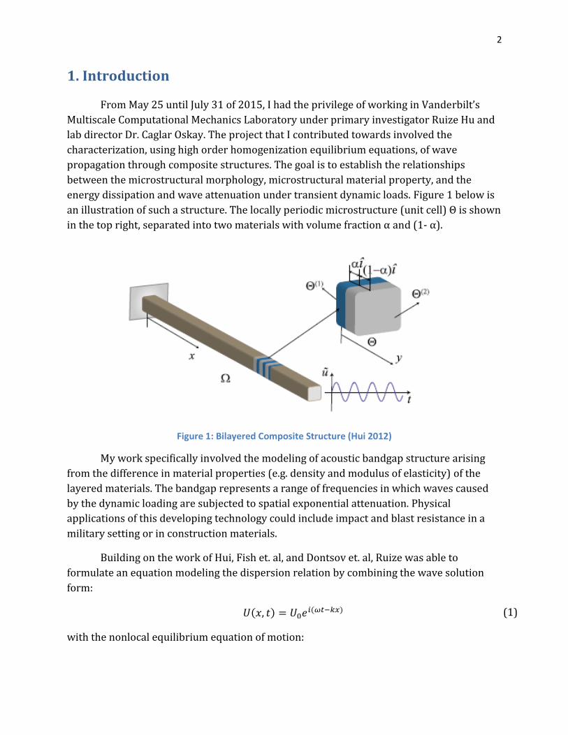
1. Introduction

From May 25 until July 31 of 2015, I had the privilege of working in Vanderbilt’s

Multiscale Computational Mechanics Laboratory under primary investigator Ruize Hu and

lab director Dr. Caglar Oskay. The project that I contributed towards involved the

characterization, using high order homogenization equilibrium equations, of wave

propagation through composite structures. The goal is to establish the relationships

between the microstructural morphology, microstructural material property, and the

energy dissipation and wave attenuation under transient dynamic loads. Figure 1 below is

an illustration of such a structure. The locally periodic microstructure (unit cell) Θ is shown

in the top right, separated into two materials with volume fraction α and (1- α).

Figure 1: Bilayered Composite Structure (Hui 2012)

My work specifically involved the modeling of acoustic bandgap structure arising

from the difference in material properties (e.g. density and modulus of elasticity) of the

layered materials. The bandgap represents a range of frequencies in which waves caused

by the dynamic loading are subjected to spatial exponential attenuation. Physical

applications of this developing technology could include impact and blast resistance in a

military setting or in construction materials.

Building on the work of Hui, Fish et. al, and Dontsov et. al, Ruize was able to

formulate an equation modeling the dispersion relation by combining the wave solution

form:

𝑈(𝑥, 𝑡) = 𝑈0𝑒𝑖(𝜔𝑡−𝑘𝑥) (1)

with the nonlocal equilibrium equation of motion:

3

𝜌02�̃�,𝑡𝑡 − 𝐸0

2�̃�,𝑥𝑥 − (𝐸𝑑 − ν𝐸0

𝐸𝑘

𝐸ℎ)

2

�̃�,𝑥𝑥𝑥𝑥 − 𝜌0 (2ν𝐸𝑘

𝐸ℎ−

𝐸ℎ

𝐸𝑑)

2

�̃�,𝑥𝑥𝑡𝑡

− 𝜌02 (

𝐸ℎ

𝐸0𝐸𝑑− ν

𝐸𝑘

𝐸0𝐸ℎ)

2

�̃�,𝑡𝑡𝑡𝑡 = 0 + 𝑂(ζ2)

(2)

resulting in the dispersion equation:

(𝐸𝑑 − ν𝐸0

𝐸𝑘

𝐸ℎ) 𝑘4 + 𝜌0 (2ν

𝐸𝑘

𝐸ℎ−

𝐸ℎ

𝐸𝑑) 𝜔2𝑘2 − 𝐸0𝑘2 + 𝜌0

2 (𝐸ℎ

𝐸0𝐸𝑑− ν

𝐸𝑘

𝐸0𝐸ℎ) 𝜔4 + 𝜌0𝜔2 = 0

(3)

where ρ0 is the homogenized density and E0 is the O(1) first order homogenized modulus.

Ed, Eh, and Ek are the homogenized moduli at O(ζ2), O(ζ4), and O(ζ6), respectively, where

O(ζi) is the homogenized macroscale equilibrium equation of order i. U0 is the displacement

amplitude, ω is the excitation frequency, and k is the wavenumber. In Eq. 2, �̃� denotes the

mean displacement field with O(ζ2) approximation, and subscript comma followed by x or t

indicate spatial derivative with respect to macroscale variables and time derivative,

respectively.

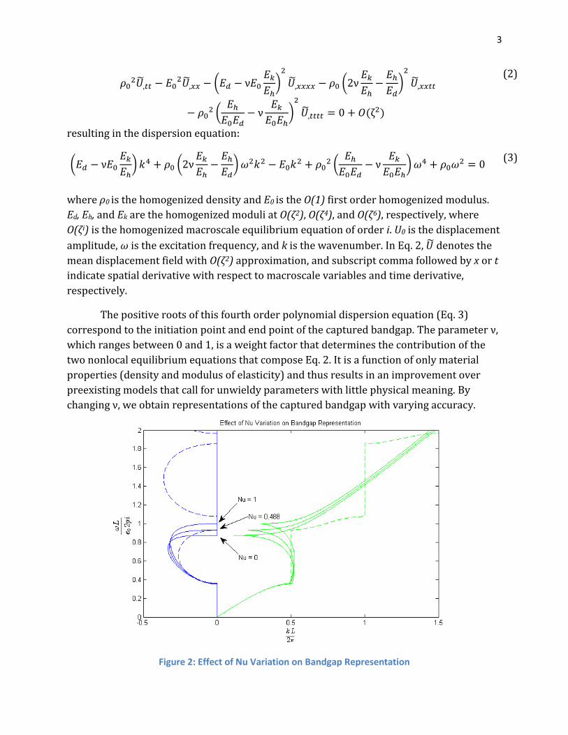
The positive roots of this fourth order polynomial dispersion equation (Eq. 3)

correspond to the initiation point and end point of the captured bandgap. The parameter ν,

which ranges between 0 and 1, is a weight factor that determines the contribution of the

two nonlocal equilibrium equations that compose Eq. 2. It is a function of only material

properties (density and modulus of elasticity) and thus results in an improvement over

preexisting models that call for unwieldy parameters with little physical meaning. By

changing ν, we obtain representations of the captured bandgap with varying accuracy.

Figure 2: Effect of Nu Variation on Bandgap Representation

4

Figure 2 is an example of the dispersion relation in a bilayer composite consisting of

aluminum and polymer layers. The vertical axis measures normalized frequency, while the

horizontal axis measures normalized wavenumber. The effects of ν variation on other cases

can be more or less drastic. The blue lines represent the imaginary solutions, and the green

lines represent the real solutions. Dotted lines represent the analytical Floquet-Bloch

model solutions that are used as reference, and solid lines represent the solutions to our

experimental model. The size of the bandgap can be determined by considering the vertical

length of the nonzero “hump” portion of the imaginary (blue) solution or the equivalent

section of real (green) solution. Essentially, the bandgap represents the range of

frequencies from a dynamic load that can be attenuated; this effect is a result of the

frequency of the dynamic load resonating with the natural frequency of the materials’

microstructure. The dispersion relations for three different cases of ν are shown (e.g. for ν

= 1, ν = 0, and ν = 0.488, which was calculated to be the value that provided the best fit).

The main objective of my project this summer was to establish a function to

determine the ν values that most closely align our experimental model with the analytical

Floquet-Bloch model for a range of material combinations. This function would ideally be

dependent on only two material properties, impedance and wave velocity, which in turn

are dependent only on density and modulus of elasticity.

5

2. Process and Results

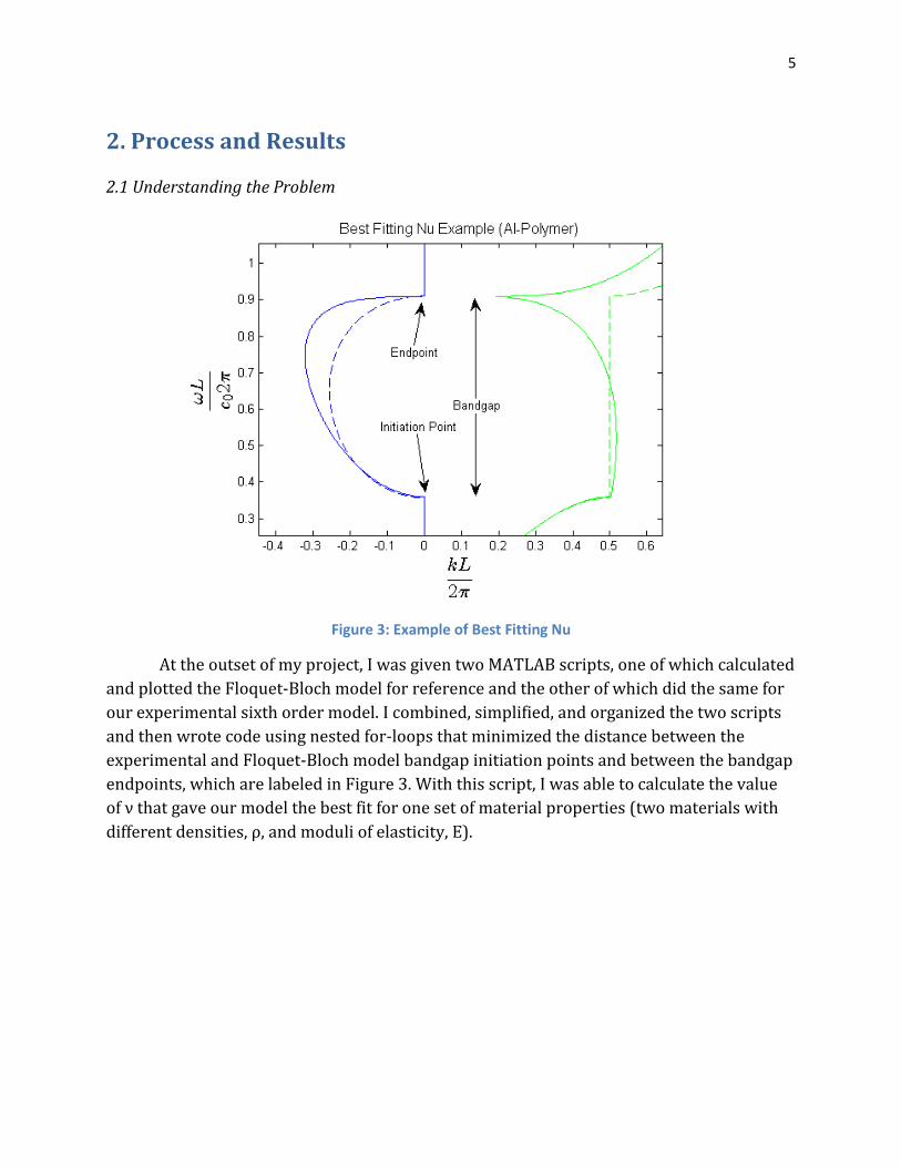
2.1 Understanding the Problem

Figure 3: Example of Best Fitting Nu

At the outset of my project, I was given two MATLAB scripts, one of which calculated

and plotted the Floquet-Bloch model for reference and the other of which did the same for

our experimental sixth order model. I combined, simplified, and organized the two scripts

and then wrote code using nested for-loops that minimized the distance between the

experimental and Floquet-Bloch model bandgap initiation points and between the bandgap

endpoints, which are labeled in Figure 3. With this script, I was able to calculate the value

of ν that gave our model the best fit for one set of material properties (two materials with

different densities, ρ, and moduli of elasticity, E).

6

Figure 4: Fit vs. Nu

Figure 4 provides a visualization of the effect that ν has on the vertical distance

between the two models’ initiation points (y1 distance) and endpoints (y2 distance) for an

example case of high-contrast aluminum layers. Note that at this point, the values of ν

ranged from around 0 to 50 instead of 0 to 1 because occurrences of the ν parameter in Eq.

2 (see Introduction) had originally been 1

1+𝜈 instead of ν. Also note that the minimum for y1

distance and the minimum for y2 distance occurred at different values of ν, meaning that

we are trying to optimize two constraints using only one parameter. Furthermore, the

range of endpoint distance is much greater than the range of initiation point distance.

2.2 Generating Best Nu Data

The next step was to generate a plot of best fitting ν values that could eventually be

curve-fitted to a function. To do this, I set the first layer material properties to be constant

while specifying a range of E2 and ρ2 values corresponding to a desired material class

found on the Ashby Plot for materials selection shown in Figure 5.

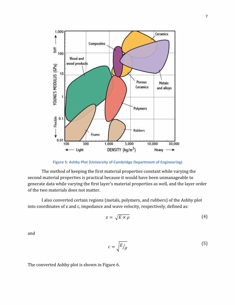
7

Figure 5: Ashby Plot (University of Cambridge Department of Engineering)

The method of keeping the first material properties constant while varying the

second material properties is practical because it would have been unmanageable to

generate data while varying the first layer’s material properties as well, and the layer order

of the two materials does not matter.

I also converted certain regions (metals, polymers, and rubbers) of the Ashby plot

into coordinates of z and c, impedance and wave velocity, respectively, defined as:

𝑧 = √𝐸 × 𝜌 (4)

and

𝑐 = √𝐸

𝜌⁄ (5)

The converted Ashby plot is shown in Figure 6.

8

Figure 6: Converted Ashby Plot

The converted Ashby plot was then used to refine the sampling process; since I was

testing for a range of both E2 and ρ2, some of the sampling points would fall outside the

boundaries of the material class. For example, the following Figure 7 shows the sampling

points for the case when the second layer was a metal. The points falling outside of the

boundaries were removed from the data.

Figure 7: Using Converted Ashby Plot to Refine Sampling Points

9

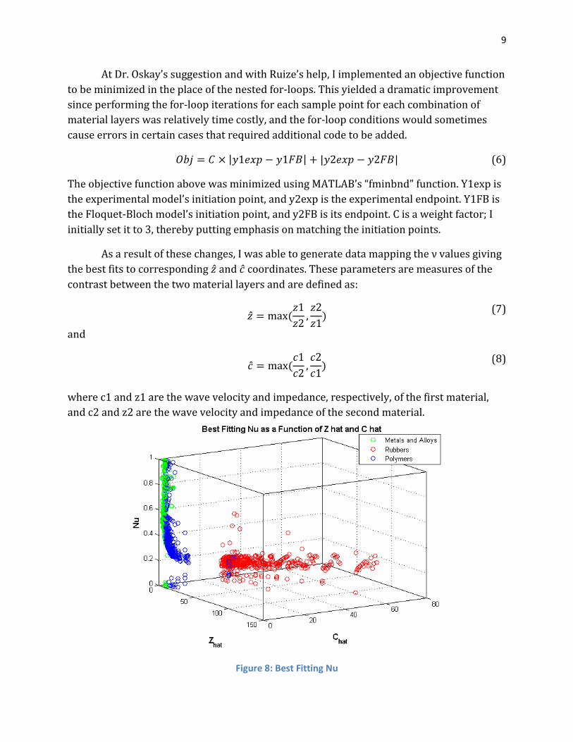
At Dr. Oskay’s suggestion and with Ruize’s help, I implemented an objective function

to be minimized in the place of the nested for-loops. This yielded a dramatic improvement

since performing the for-loop iterations for each sample point for each combination of

material layers was relatively time costly, and the for-loop conditions would sometimes

cause errors in certain cases that required additional code to be added.

𝑂𝑏𝑗 = 𝐶 × |𝑦1𝑒𝑥𝑝 − 𝑦1𝐹𝐵| + |𝑦2𝑒𝑥𝑝 − 𝑦2𝐹𝐵| (6)

The objective function above was minimized using MATLAB’s “fminbnd” function. Y1exp is

the experimental model’s initiation point, and y2exp is the experimental endpoint. Y1FB is

the Floquet-Bloch model’s initiation point, and y2FB is its endpoint. C is a weight factor; I

initially set it to 3, thereby putting emphasis on matching the initiation points.

As a result of these changes, I was able to generate data mapping the ν values giving

the best fits to corresponding �̂� and �̂� coordinates. These parameters are measures of the

contrast between the two material layers and are defined as:

�̂� = max (

𝑧1

𝑧2,𝑧2

𝑧1)

(7)

and

�̂� = max (

𝑐1

𝑐2,𝑐2

𝑐1)

(8)

where c1 and z1 are the wave velocity and impedance, respectively, of the first material,

and c2 and z2 are the wave velocity and impedance of the second material.

Figure 8: Best Fitting Nu

10

Figure 8 shows best fitting ν data for combinations of aluminum and metals/alloys,

aluminum and polymers, and aluminum and rubbers. Here the range of ν is between 0 and

1.

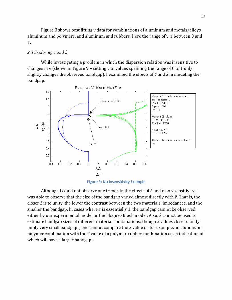
2.3 Exploring �̂� and �̂�

While investigating a problem in which the dispersion relation was insensitive to

changes in ν (shown in Figure 9 – setting ν to values spanning the range of 0 to 1 only

slightly changes the observed bandgap), I examined the effects of �̂� and �̂� in modeling the

bandgap.

Figure 9: Nu Insensitivity Example

Although I could not observe any trends in the effects of �̂� and �̂� on ν sensitivity, I

was able to observe that the size of the bandgap varied almost directly with �̂�. That is, the

closer �̂� is to unity, the lower the contrast between the two materials’ impedances, and the

smaller the bandgap. In cases where �̂� is essentially 1, the bandgap cannot be observed,

either by our experimental model or the Floquet-Bloch model. Also, �̂� cannot be used to

estimate bandgap sizes of different material combinations; though �̂� values close to unity

imply very small bandgaps, one cannot compare the �̂� value of, for example, an aluminum-

polymer combination with the �̂� value of a polymer-rubber combination as an indication of

which will have a larger bandgap.

11

Figure 10: Z hat Effect on Bandgap Size

Figure 11: C Hat Effect on Bandgap Size

Figures 10 and 11 show the effects of �̂� and �̂� on the bandgap size for an aluminum-

metals/alloys combination. In order to avoid the surface plot “folding back” on itself, for

this scenario �̂� was defined to be z1/z2, and �̂� was defined to be c1/c2. As can be observed

12

in Figure 10, the further �̂� is from unity (i.e. the greater the contrast), the larger the

bandgap size. However, not much could be concluded about the effect of �̂�.

Figure 12: Z Hat and C Hat Effect on Bandgap Size

Figure 13: Z Hat Effect on Bandgap Size

Figures 12 and 13 corroborate these findings; Figure 12 shows �̂� and �̂� effect on

bandgap size for a combination of rubber-metal, and Figure 13 is a cross section of Figure

12 with �̂� held constant. Again, the definitions of �̂� and �̂� were defined for this case to be

z1/z2 and c1/c2. Clearly, greater contrast in impedance means larger bandgap size.

13

2.4 Best Fitting Nu Data

Figure 14: Best Nu vs. Z hat and C hat

Figure 14 is a plot of the ν values that gave our experimental model the most

accurate dispersion relation (in comparison to the Floquet-Bloch reference model) against

coordinates of �̂� and �̂�, which are defined as they originally were in section 2.2, page 9. I

also added material combinations of rubber-polymers, polymer-rubbers, and lead-metals

to the data. Each set of data contains between 260 and 330 data points.

Figure 15: Error vs. Z hat and C hat

14

Figure 15 shows the associated error with each data point calculated by the

formula:

𝛹 = √(𝑦1𝑒𝑥𝑝 − 𝑦1𝐹𝐵)2 + (𝑦2𝑒𝑥𝑝 − 𝑦2𝐹𝐵)2

(𝑦1𝐹𝐵)2 + (𝑦2𝐹𝐵)2

(9)

where y1exp and y2exp are our experimental model’s initiation points and endpoints,

respectively, and y1FB and y2FB are the Floquet-Bloch model’s initiation points and

endpoints, respectively. The combinations of aluminum-metals, lead-metals, and polymer-

rubbers yielded errors that were undesirably high, and upon investigation, I observed a

problem that was common to the three combinations. Since our objective function (page 9)

included a weight factor on the initiation point, the calculated best fitting ν value would

often give a highly accurate initiation point at the expense of a comparably much more

inaccurate endpoint (recall from Figure 4, page 6, that the range of endpoint distance was

much higher than the range of initiation point distance).

Figure 16: Example of High Error Due to Weight Factor

Shown in Figure 16, the calculated best ν value of 0.382 gave an error of 12.85%

while a ν value of 0.15 resulted in an error of just 2.22%. Since this problem was common

to the high error cases, I decided to eliminate the weight factor and recalculate the data.

The resulting plot of best ν values can be seen in Figure 17, and the associated error plot in

15

Figure 18.

Figure 17: Best Nu with Equally Weighted Initiation Point and Endpoints

Figure 18: Equal Weighted Error vs. C hat and Z hat

Clearly, many of the high error cases in aluminum-metal, polymer-rubber, and lead-

metal combinations were resolved; however, there were still stubborn aluminum-metal

cases that yielded error between 12% and 16%. This is because of a problem with

16

insensitivity (see Figure 9, page 10) in which the entire range of ν values only slightly

changes the experimentally modeled bandgap.

Besides these instances, one can observe that, for �̂� values around 1, the error is

higher (around 10%) for aluminum-metal and lead-metal combinations. This is because of

the miniscule bandgap size due to the low impedance contrast; our model has difficulty

approximating the bandgap in such cases as seen in Figure 19. Although the error actually

increased slightly after eliminating the weight factor in this example case, the advantage of

this change is still evident in the lower error results for the majority of cases.

A relatively high error case of a polymer-rubber combination is shown in Figure 20.

In certain cases, our experimental model is simply unable to capture both the initiation

point and the endpoint; however, it still provides a reasonable approximation of the

bandgap, and the error is still an acceptable 8.41%.

Also, note that the calculated best ν values for polymer-rubber and rubber-polymer

combinations were very similar (see Figure 17), as was expected. However, polymer-

rubber combinations had somewhat higher errors than did rubber-polymer combinations.

This is understandable since each case of rubber-polymers is not necessarily the opposite

of each case of polymer-rubbers; the rubber layer in rubber-polymers and the polymer

layer in polymer-rubbers were chosen arbitrarily in their respective material classes

according to the Ashby materials selection plot (see Figure 5, page 7).

Figure 19: Small Bandgap Issue

17

Figure 20: Example of Polymer-Rubbers High Error

2.5 Curve Fitting

Using MATLAB’s curve fitting toolbox, I was able to establish a function ν(�̂�, �̂�) that

provides an approximation of the best fitting ν for a specified �̂� and �̂�, which can be

calculated for any bilayer composite structure. I originally fit the function to the best ν data

in Figure 17 but found that the function-projected ν values for aluminum-metals yielded

error up to 30%. Excluding the aluminum-metals best ν data, I refit the function to be:

𝜈(�̂�, �̂�) =

1

−0.6181 × �̂� + 2.559 × �̂�+ 0.1161

(10)

where the coefficients were determined through nonlinear least squares method. This

function provides a reasonable approximation of the ν value that gives the most accurate

model of the bandgap for the combinations of materials tested. I believe it can be used for

many other combinations as well, although it is more unreliable for low contrast cases,

such as when the two layers are composed of materials from the same class (e.g.

aluminum-metals). For these situations, I would advise cautious use of 𝜈(�̂�, �̂�) or even

direct, programmatic calculation. Also bear in mind that this function has been tested only

when the volume fraction α = 0.5 and the unit cell length l = 0.01 m. The following table

displays the minimum, maximum, mean, and standard deviation in error (decimal)

associated with the ν values calculated using 𝜈(�̂�, �̂�) for the combinations of materials

tested.

18

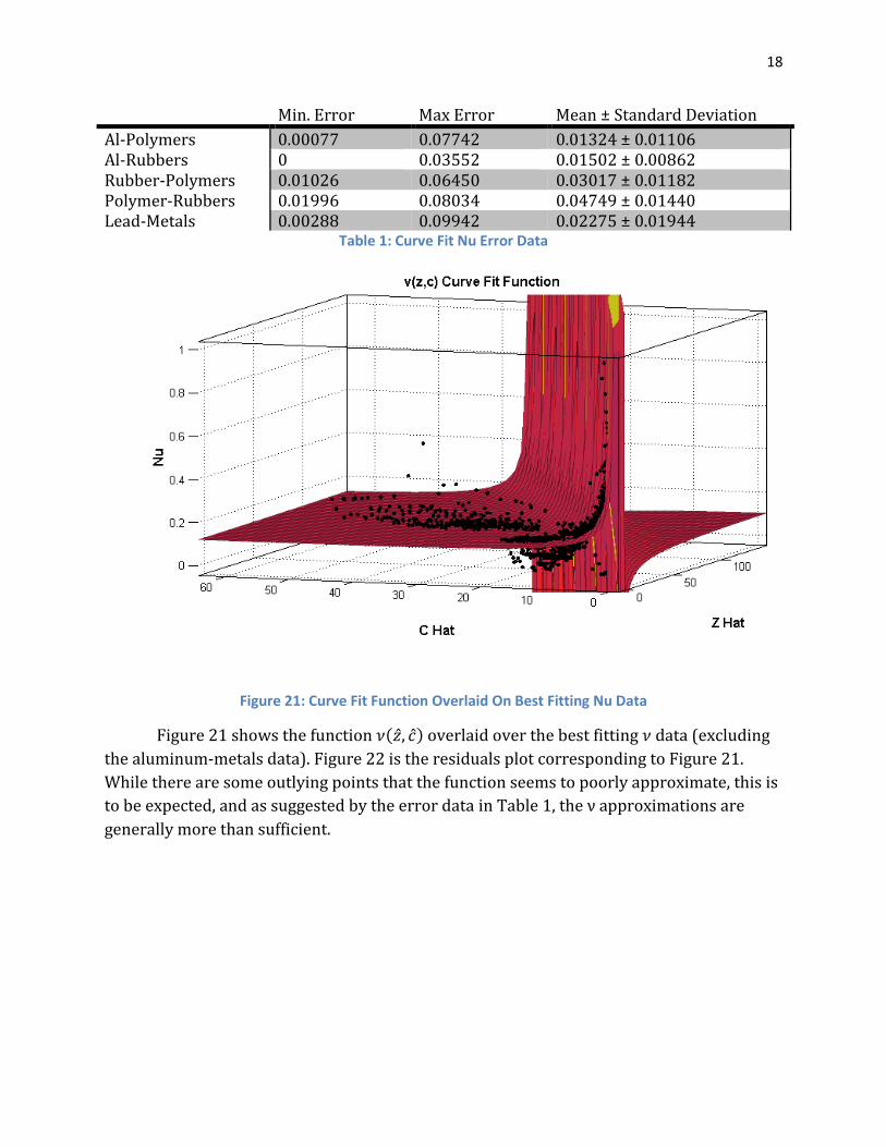
Min. Error Max Error Mean ± Standard Deviation

Al-Polymers 0.00077 0.07742 0.01324 ± 0.01106 Al-Rubbers 0 0.03552 0.01502 ± 0.00862 Rubber-Polymers 0.01026 0.06450 0.03017 ± 0.01182 Polymer-Rubbers 0.01996 0.08034 0.04749 ± 0.01440 Lead-Metals 0.00288 0.09942 0.02275 ± 0.01944

Table 1: Curve Fit Nu Error Data

Figure 21: Curve Fit Function Overlaid On Best Fitting Nu Data

Figure 21 shows the function 𝜈(�̂�, �̂�) overlaid over the best fitting 𝜈 data (excluding

the aluminum-metals data). Figure 22 is the residuals plot corresponding to Figure 21.

While there are some outlying points that the function seems to poorly approximate, this is

to be expected, and as suggested by the error data in Table 1, the ν approximations are

generally more than sufficient.

19

Figure 22: Residuals Plot of Curve Fit Function

20

Conclusions

3.1 Summary

Given a pair of MATLAB scripts that calculated and plotted the dispersion relations

for the Floquet-Bloch model and for our experimental sixth order model, I was able to

establish a function 𝜈(�̂�, �̂�) that returns the parameter 𝜈 value giving our experimental

model the closest fit with the reference Floquet-Bloch model. The 𝜈(�̂�, �̂�) projected 𝜈 values

yield up to 10% error but will more typically yield error closer to 3 to 4%. This function

has been successful for combinations of aluminum-polymers, aluminum-rubbers, rubber-

polymers, polymer-rubbers, and lead metals where the volume fraction α = 0.5 and the unit

cell length l = 0.01 m. However, it yields relatively high error for the aluminum-metals

combination, and in general, combinations of materials from the same class yield higher

errors. I was also able to create a graphic representation of the effect of the impedance

parameter �̂� on bandgap size; greater contrast in �̂� implies larger bandgap size.

3.2 Future Work

The next step in this research involves implementing three or more layers of

materials into the sixth order model in 1D, ultimately working up to the 3D core shell

structure shown in Figure 23 and Figure 24.

Figure 23: Composite Structures (Maldovan)

Figure 24: Core Shell Structure (Liu, et al.)

21

3.3 Personal Reflection

My experience conducting an undergraduate summer research project at

Vanderbilt’s Multiscale Computational Mechanics Laboratory has been an educational and

valuable one. The majority of my technical work was done in MATLAB, and through the

course of my fellowship, I have observed a marked improvement in my capabilities with

the program. In terms of personal development, I now have a decent grasp of what it is like

to work in a research environment, a result of both my own project and daily interactions

with the lab’s staff. Furthermore, I gained experience in managing myself as far as setting

concrete daily and weekly objectives, comparing my progress to these objectives, and

recording and organizing my data and figures.

22

References Egor V. Dontsov, Roman Tokmashev, Bojan B. Guzina. "A physical perspective of the length scales in

gradient elasticity through the prism of wave dispersion." International Journal of Solids and

Structures, 2013: 50(22):3674-3684.

Jacob Fish, Wen Chen, Gakuji Nagai. "Non-local dispersive model for wave propagation in

heterogeneous media: multi-dimensional casedimensional case." International Journal for

Numerical Methods in Engineering, 2002: 54(3):347-363.

Jacob Fish, Wen Chen, Gakuji Nagai. "Non-local dispersive model for wave propagation in

heterogeneous media: one-dimensional case." International Journal for Numerical Methods in

Engineering, 2002: 54(3).

Maldovan, Martin. "Sound and heat revolutions in phononics." Nature, 2013.

Tong Hui, Caglar Oskay. "A nonlocal homogenization model for wave dispersion in dissipative composite

materials." International Journal of Solids and Structures, 2013: 50(1):38-48.

University of Cambridge Department of Engineering. Young's Modulus - Density. 2002. http://www-

materials.eng.cam.ac.uk/mpsite/interactive_charts/stiffness-density/NS6Chart.html.

Zhengyou Liu, Xixiang Zhang, Yiwei Mao, Y. Y. Zhu, Zhiyu Zhang, C. T. Chan, Ping Sheng. "Locally resonant

sonic materials." Science, 2000.