University of North FloridaUNF Digital Commons

Management Faculty Publications Department of Management

8-2010

Voter Bias in the Associated Press College FootballPollB. Jay ColemanUniversity of North Florida, jcoleman@unf.edu

Andres GalloUniversity of North Florida, agallo@unf.edu

Paul MasonUniversity of North Florida, pmason@unf.edu

Jeffrey W. SteagallUniversity of North Florida, jsteagal@unf.edu

Follow this and additional works at: http://digitalcommons.unf.edu/bmgt_facpub

Part of the Management Sciences and Quantitative Methods Commons

This Article is brought to you for free and open access by the Departmentof Management at UNF Digital Commons. It has been accepted forinclusion in Management Faculty Publications by an authorizedadministrator of UNF Digital Commons. For more information, pleasecontact Digital Projects.© 8-2010 All Rights Reserved

Recommended CitationColeman, B. Jay; Gallo, Andres; Mason, Paul; and Steagall, Jeffrey W., "Voter Bias in the Associated Press College Football Poll"(2010). Management Faculty Publications. 4.http://digitalcommons.unf.edu/bmgt_facpub/4

VOTER BIAS IN THE ASSOCIATED PRESS COLLEGE FOOTBALL POLL

Submitted by

B. Jay Coleman, Ph.D.

(Contact Author) Department of Management Coggin College of Business University of North Florida

1 UNF Drive Jacksonville, Florida 32224-7699

(904) 620-1344 (904) 620-2782 FAX

E-mail: jcoleman@unf.edu

Andres Gallo, Ph.D. Department of Economics & Geography

Coggin College of Business University of North Florida

1 UNF Drive Jacksonville, Florida 32224-7699

(904) 620-1694 E-mail: agallo@unf.edu

Paul Mason, Ph.D.

Department of Economics & Geography Coggin College of Business University of North Florida

1 UNF Drive Jacksonville, Florida 32224-7699

(904) 620-2640 E-mail: pmason@unf.edu

Jeffrey W. Steagall, Ph.D.

Department of Economics & Geography Coggin College of Business University of North Florida

1 UNF Drive Jacksonville, Florida 32224-7699

(904) 620-2395 E-mail: jsteagal@unf.edu

To

Journal of Sports Economics

- 2 -

VOTER BIAS IN THE ASSOCIATED PRESS COLLEGE FOOTBALL POLL

Abstract

We investigate multiple biases in the individual weekly ballots submitted by the 65 voters

in the Associated Press college football poll in 2007. Using censored tobit modeling, we find

evidence of bias toward teams (1) from the voter’s state, (2) in conferences represented in the

voter’s state, (3) in selected Bowl Championship Series conferences, and (4) that played in

televised games, particularly on relatively prominent networks. We also find evidence of

inordinate bias toward simplistic performance measures – number of losses, and losing in the

preceding week – even after controlling for performance using mean team strength derived from

16 so-called computer rankings.

Keywords: Discrimination, Voting, Group Decisions, Football, Censored Tobit

Acknowledgement: We wish to acknowledge the substantial assistance provided by the two anonymous referees, and thank them for their valuable contributions to the improvement of this research.

- 3 -

VOTER BIAS IN THE ASSOCIATED PRESS COLLEGE FOOTBALL POLL

I. Introduction

Without anything beyond a two-team playoff tournament, the national champion of the

NCAA’s Football Bowl Subdivision (or FBS, formerly known as Division 1-A), as well as the

teams that are eligible to play in the Bowl Championship Series (BCS) national championship

game, is selected or designated through various polls and/or mathematical ranking systems.

Since its inception in 1936, the Associated Press (AP) college football poll has been one of the

two most widely recognized rankings in the sport. (The so-called “coaches poll,” first presented

under the auspices of United Press International (UPI) in 1950, and which has been under the

purview of USA Today and/or ESPN since 1997, is the other.) Consequently, the AP poll’s

“national champion” (or top-rated team) in its final, post-bowl poll is one of the two most widely

recognized such designations, and is therefore highly prized among the (currently) 119 FBS

schools. It is also one of only four rankings that are formally recognized by the NCAA on its

web site (NCAA, 2008). Moreover, from 1998 through 2004, the AP poll was included in the

BCS composite ranking, meaning that during that period it had direct impact on who had the

opportunity to play in the national championship game (Carey and Whiteside, 2004).

The AP poll, which currently includes the top 25 teams, is compiled and distributed

weekly during the season and then once again after all post-season bowl games have been

played. It is actually a composite of the individual rankings of (currently) 65 sportswriters and

broadcasters dispersed across the nation, each of whom submits his/her respective top 25 each

week. For the 2007 season, four of the 65 voters were members of the national media (from

ESPN, ABC, SI.com, and College Sports Television), and the other 61 were associated with

- 4 -

local newspapers, radio stations, and television stations in 41 states. Only two states (California

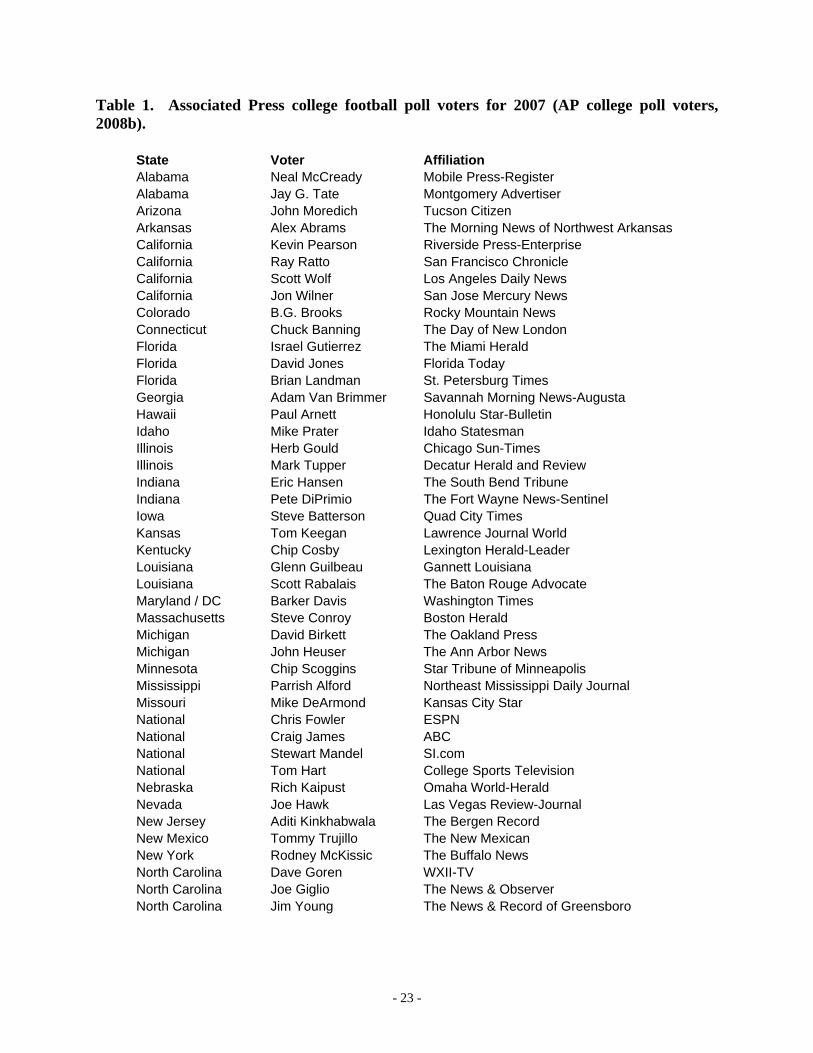
and Texas) were represented by as many as four voters each. Table 1 contains the list of AP

poll voters for the 2007 season, together with their respective affiliations and locations.

Because of the geographic distribution of voters, and the virtual impossibility that a voter

is able to watch all teams play in any given week, voters may be inclined to give more favorable

treatment to those teams for which they have more information, and/or toward teams (or fans of

teams) with whom they are affiliated. There are numerous ways in which familiarity or

affiliation may be increased. Voters are likely more familiar (and more closely affiliated) with

teams that are in the same geographic vicinity and/or in the same state as the voter, and/or with

teams that participate in the same conference (or league) as those teams in the voter’s vicinity.

Familiarity with teams is also generated through televised games, and teams not

appearing on major networks may suffer by comparison. In addition, teams that are members of

the six BCS leagues – those leagues whose champion receives an automatic bid to one of the

BCS bowls – generally receive greater publicity than non-BCS conference members, and this

might generate favor in balloting. Teams that actually played during the preceding week had the

opportunity to be before the eyes of voters more readily than those which had a bye week. Also,

some voters are affiliated with networks (e.g., ESPN) that televise various games in a given

week, meaning that teams playing on such networks may have a higher degree of familiarity (or

even affiliation) with affiliated voters versus teams that do not. Finally, in addition to simply

having more familiarity with various teams, sportswriters and broadcasters may also be swayed

by the implicit desire to please the primary audiences for (or to) whom they write and speak

(Reinardy, 2004).

- 5 -

Indeed, the Associated Press is cognizant of such issues, as evidenced by guidelines sent

out by the AP itself, warning voters to “base your vote on performance, not reputation or

preseason speculation,” to “avoid regional bias, for or against,” to avoid “homerism,” and to

avoid affiliations with boosters or taking inducements that could be construed as being

associated with voters (Donahue, 2005).

In this paper, we seek to examine the presence of the forms of bias described above using

the individual ballots submitted by the 65 AP poll voters during the last nine weeks of 2007. All

prior published research on the AP poll has suffered from a lack of availability of the individual

ballots of each voter. Any and all assessments of bias have been forced instead to use the weekly

aggregate of all ballots – i.e., the collective poll published each week – as the unit of analysis.

This data availability problem was allayed starting in 2006, when for the first time the

Associated Press began regularly publishing on the Web the individual ballots of all participating

voters. Although votes were apparently not archived in such a way for observers to view

anything other than the ballots from the most recent week, for the first time a much more

granular level of data was made available to the public. This level of detail allows for the

scrutiny of the geographic bias of voters beyond any previous research, and it is the unit of

assessment we employ here.

II. Literature Review

Concerns about poll voter bias are prevalent in the popular literature. As of July 2008, a

Google search for web sites including all the terms “Associated Press college football poll bias”

yielded more than 33,000 results. Many of these appear to be articles about the flaws in the BCS

ranking system, but a large number relate to regional or conference (or other) biases in how

voters rank the top 25 teams. As examples, consider:

- 6 -

This is the dirty little secret of football polls. A reporter can cover only one game each Saturday, but still assumes the role of an authority in ranking the top 25 teams, based on the abridged evidence of television highlights and newspaper accounts, and the bias of regional favoritism. … Meanwhile, tens of millions of dollars in bowl invitations rest on flimsy decisions (Longman, 2002). Reporters and columnists are entitled to their opinion, but if they are going to insist on flashing regional bias, I think fans should insist that these folks not be given the responsibility – the privilege, actually – of having such sway over a process that is more a national trust of fandom than personal fiefdom of a couple dozen newspaper reporters (Shanoff, 2006). In response to Shanoff’s sentiment, Dan Steinberg of washingtonpost.com performed an

assessment of the AP voting during one week and concluded (unscientifically) that he could not

find any specific regional bias: “for every example of a horribly over-rated Pac-10 team by a

voter in a Pac-10 town, there was a Big-10 team surprisingly undervalued by a voter in a Big-10

market” (Steinberg, 2006). In 2001, Ted Miller at CNNSI.com discussed the possible easing of

the perceived East Coast bias relative to the Pacific 10 (Pac-10) conference, pointing out that of

the 72 AP voters in 2001 California had four voters while Florida had only three. However, he

notes that voters in the East often go to bed before West Coast night games conclude, and that

East Coast-based papers and national highlight shows are often devoid of coverage of such

games. Moreover, he points to the virtually religious nature of college football in the South,

which can lead to responses by the media to the “conventional wisdom” that players there are

“tougher than those out West because they care more.” He also mentions a familiarity influence

that potentially benefits schools that are consistently dominant year-to-year (Miller, 2001).

The scholarly literature has less to say about bias in college football polls, although there

is substantial literature examining various poll characteristics. Libovic and Sigelman (2001)

provide an overview of the ranking literature prior to 2000 vis-à-vis college football. As they

note, Tsai and Sigelman (1980) demonstrate the limited availability of top 10 positions to teams

- 7 -

not so ranked in the previous season, and Goff (1996) showed that pre-season rankings impact

those at the end of the season, regardless of results over the course of the season.

In addition, Goff’s work tested for the presence of bias toward each of the 46 individual

teams in his analysis (which covered 1980-1989), as well as collectively toward teams from the

Big 10 conference (including Notre Dame in that grouping). He found no preference toward the

Big 10 in general, but found possible team-specific bias in favor of Big 10 schools Ohio State,

Michigan, and Michigan State, as well as relatively unfavorable treatment of Air Force,

Clemson, Georgia Tech, Syracuse, and Texas Tech.

Libovic and Sigelman (2001) use logistic regression to study the AP polls from 1985

through 1995, to determine the factors that cause teams to move up after a win. They find that

having one loss, having two or more losses, the current ranking position, whether an opening

occurs higher in the ranking, the type of win (e.g., over a higher- or lower-ranked opponent), and

the change in the ranking of earlier opponents all are related to the ability of a winning team to

improve its ranking. These authors also conclude that the predictive performance of AP voters

does not improve as the season progresses.

Stern et al. (2004) provide a thorough review of the development of the BCS system and

the elements of it. They reference the beginnings of the AP poll and how its coexistence with the

UPI poll drove the diversity of opinion and controversy regarding the national champions that

pre-dated the BCS. They note the inherent biases and shortcomings associated with the polls,

and point to the BCS and mathematical ranking systems as attempts to rank teams while

eliminating or at least reducing such biases.

Callaghan, Mucha, and Porter (2004) review the BCS system – in the process also noting

accusations of bias in the polls – and suggest that there is significant double-counting of factors

- 8 -

such as schedule strength, numbers of losses, and quality wins. They propose the likelihood that

a simple random walk methodology that they refer to as “a collection of trained monkeys” can

generate rankings as good as those provided by currently available systems.

Coleman (2005) shows that none of the upwards of 100 ranking systems posted on the

Web from 2000 through 2003 approached the goal of minimizing the number of game score

violations (or reversals): cases in which the winner of a previous game is ranked below the team

it defeated. All systems contained violations that were at least 38% higher than the minimum.

He also specifically addressed the top 5 of the AP poll in 1994 and 1995, and concluded that a

minimum violations criterion would have changed the top 5 AP teams in 1994. Using a similar

approach, he determined that a minimum violations criterion would have replaced Nebraska with

Oregon in the 2001 BCS championship game – a result that would have actually matched the AP

poll (and the coaches’ poll) in that season, but which was reversed by the computer rankings that

were included in the BCS computations.

Campbell, Rogers, and Finney (2007) specifically address the bias question by looking at

the AP poll in the 2003-04 and 2004-05 seasons. They find that a team’s television exposure

above the norm is a significant factor in AP voting results. As part of their analysis, they also

test for the presence of bias toward teams from BCS conferences, as well as bias associated with

each specific team in their study (the latter being also a possible measure of bias associated with

market size). They conclude that AP voters do not have biases associated with particular teams.

They also find no bias associated with whether a team is from a BCS conference; however,

playing an opponent in a BCS conference is significant, although likely as a proxy for opponent

strength.

- 9 -

Paul, Weinbach, and Coate (2007) also emphasize the role of television, but they

question whether TV exposure drives the voters in the polls, or whether the poll ranking directs

networks to televise the games that are perceived to be most important. Of the seven national

networks they examine, they find that games televised on six of the seven (excepting only NBC)

were related in some way to AP poll votes. They also find that televised and non-televised losses

carry greater weight than wins, with the effects of wins and losses somewhat magnified by

television. However, these authors place emphasis on the gambling point-spreads as

determinants of rankings, given the nature of spreads as measures of market (or voter)

expectation. They conclude that performance vis-à-vis the spread is a significant driver of how

teams fare in the polls.

Finally, Logan (2007) employs 25 years of AP voting to address three common

perceptions of biases in the polls. He emphasizes losses early or late, strength of defeated

opponents and winning margin. His conclusions are contrary to the typical expectations relative

to those biases, suggesting that it is better to lose later than earlier, strength of a defeated

opponent is irrelevant, and margin of victory is irrelevant.

III. Data and Variables We collected the ballot submitted by each AP poll voter for each of the final nine polls

(i.e., polls 8 through 16) of the 2007 season (AP college poll voters, 2007, 2008a). Starting our

analysis roughly halfway through the season to some extent mitigated starting condition or

minimal sample size effects associated with pre-season and early-season rankings, because by

that point voters had received a reasonable opportunity to evaluate teams during the current

season. The first of these (poll 8) covered the slate of games ending on Saturday, October 13.

The final poll (poll 16) covered all regular season and post-season bowl games, through the BCS

- 10 -

national championship game on Monday, January 7, 2008. These data comprised 14,625

observations of ranked teams: 25 ranked teams for each of 65 voters for each of nine weeks. We

reverse-coded the value assigned to each ranked team by the respective voter, so that the top-

ranked team was assigned a value of 25, the second-ranked team was assigned a value of 24, etc.,

with the 25th-ranked team receiving a value of 1. This approach is comparable to the manner in

which the AP aggregates the 65 individual ballots into the collective poll. It also allowed us to

refer to higher-ranked teams as those with higher values, thereby making interpretation of results

more straightforward.

In order to allow comparison of those teams receiving votes and those teams that did not,

to each voter’s ballot in each week we added information on the 95 FBS teams that did not

receive a top 25 vote (i.e., did not appear anywhere in the top-25 ballot) from that voter.1 Each

of these teams was assigned a value of zero. Complicating this process somewhat was the fact

that on two occasions a voter included a member of the Football Championship Subdivision (or

FCS, formerly known as Division 1-AA) in his top-25 ballot for the week: Appalachian State

was included on one occasion, and Northern Iowa was included on another. Because of this

anomaly, for the sake of our analysis these two teams were treated as members of the FBS,

meaning they were included in our data set with values of zero in all cases in which they were

unranked by a voter. This inclusion raised the total number of teams examined to 122.

This data collection process generated a total sample size of 71,370 observations: 122

teams for each of the 65 voters, for each of the nine weeks examined. In order to test for our

hypothesized biases, for each of these observations we collected a variety of additional

information, which is summarized in Table 2 and detailed below.

1 There were 120 FBS teams in 2007, including Western Kentucky University, which was on probationary status during its transition to the FBS.

- 11 -

The first three were designed to capture familiarity bias associated with a voter’s

location. Using the state in which the respective voter was located (Table 1), we constructed a

binary variable reflecting whether the team named in that observation was located in the same

state as the voter. We constructed another binary variable reflecting whether the team was in a

conference that was represented in that voter’s state. (Steinberg (2006) used similar factors in

his unscientific one-week assessment during that season.) For example, a voter located in South

Carolina has teams from both the Atlantic Coast Conference (ACC) – Clemson University – and

the Southeastern Conference (SEC) – the University of South Carolina – in his/her state. Thus,

such a voter is likely quite familiar with teams from both the ACC and the SEC, given that teams

in his/her state compete on a regular basis with other teams from those conferences, and s/he

perhaps even covers events involving those teams. This binary variable thus captures a

familiarity bias in favor of such teams, and it may also capture a larger and more general regional

bias on the part of the voter (e.g., toward eastern or southeastern teams in this example).

In addition, and because voters may be also quite familiar with teams in nearby states, we

computed the distance in miles between the voter in that observation and the team named in the

observation. In each case, we used the zip code of the voter’s employer and the zip code of the

school to identify the latitude and longitude of each party, and then calculated the straight-line

geographic distance between the two using trigonometric methods.

Following the lead of Campbell, Rogers, and Finney (2007) and Paul, Weinbach, and

Coate (2007), a second set of bias factors was constructed to capture familiarity bias associated

with television coverage afforded to teams. We collected information on all games televised

during the season from (College football weekly TV schedules, 2008). Given the large number

of games that are televised in some capacity – 633 games involving at least one of the 122 teams

- 12 -

in our data set were televised during the 2007 season – and the differences in availability to

voters as a result of the market penetration of various outlets, we differentiated television

coverage by the network on which it was aired.2 We constructed five binary variables reflecting

whether a team appeared in a game televised on a given type of network during the most recent

week, including variables for national networks (ABC, CBS, FOX, and NBC), major ESPN

networks (ESPN and ESPN2), other ESPN networks (ESPN Classic, ESPN Plus, ESPNU, and

ESPN Gameplan), other major cable outlets (Fox Sports Net (FSN), the Big Ten Network,

Versus, and NFL Network), and major regional networks (Lincoln Financial Sports, Raycom

Sports, and The Mtn. (the MountainWest Sports Network)). A sixth binary variable reflected

whether a team appeared on any other television outlet. Note that in many cases games

appearing on ESPN Gameplan were also aired by other outlets (e.g., ACC or SEC games aired

by Raycom or Lincoln Financial Sports in the eastern and southeastern regions were often

available also on ESPN Gameplan in other regions of the country).

These binary variables captured a familiarity bias associated with the team playing a

televised game during the most recent week. Moreover, and similar to the approach of

Campbell, Rogers, and Finney (2007), we also wished to examine any cumulative familiarity

effect of a team appearing in televised games. To do so, we constructed six variables reflecting

the number of televised games in which the respective team had appeared up to that point in the

season on that type of network, but not including the week in question.

A third set of variables captured familiarity bias associated with whether a voter has the

opportunity to see a team play the week before casting a ballot. One binary variable represented

whether a team even played during the most recent week, and another reflected whether the team

2 This was similar to the approach of Paul, Weinbach, and Coate (2007), which employed seven binary variables with each representing a particular national network.

- 13 -

lost during the most recent week. The latter was partially spurred by the work of Lebovic and

Sigelman (2001), which indicated that AP poll voters consider the number of losses when

determining poll movements. Goff (1996) showed that the number of losses was a highly

significant factor in AP rankings. The results of Paul et al. (2007) emphasized a greater effect

from losses than wins for both televised and non-televised games. Moreover, Lebovic and

Sigelman (2001) suggested that there was a cumulative effect of losses. Thus, we also

constructed – in part as a control variable, but also as a measure of bias toward simplistic

performance measures – two variables reflecting the cumulative number of losses for that team

up through the most recent week. Similar to Lebovic and Sigelman, the first was a binary

variable reflecting whether a team had at least one loss by that point in the season. The second

reflected the number losses beyond one by that point in the season.3 As discussed below, we

included in our analysis a much more complex and comprehensive control variable for team

performance. Thus, the significance of either the number of team losses or whether a team lost

in the most recent week could reflect a bias toward quite simplistic performance measures on the

part of voters.

A fourth set of variables was constructed to capture any bias toward teams in each of the

six Bowl Championship Series (BCS) conferences: the ACC, the Big 10, the Big 12, the Big

East, the Pac-10, and the SEC. As noted earlier, the champions of these conferences each

receive automatic bids to play in one of the BCS bowls, which are the highest-paying of all post-

season games. Members of these leagues, along with independent Notre Dame (which receives

3 For example, if a team had three losses at the time of a given ballot being submitted, the first variable took a value of 1, and the second variable took a value of 2. This approach differed somewhat from Libovic and Sigelman (2001), who used a binary representing whether a team had exactly one loss, and another reflecting whether it had two or more. It also differed somewhat from the work of Goff (1996), which used the total number of losses as a predictor. Our choice of variables allowed for the differential treatment of the first loss versus losses thereafter, as well as the differential treatment of teams with two or more losses.

- 14 -

an automatic BCS bid if it wins a particular number of games), are generally considered the most

significant football-playing schools.4

As a final measure of possible bias, we constructed two variables reflecting whether those

three voters employed by ESPN, and who appear regularly on ESPN football broadcasts, were

biased toward teams appearing on any of the ESPN family of networks. ESPN was the only

media entity represented by three voters, and is the most significant television entity in college

football. As noted in Table 1, two of these voters – Chris Fowler and Craig James – are

designated by the Associated Press as “national” voters, with no state designation. (Note that

although Craig James’ affiliation is listed as “ABC,” that network owns ESPN, and James

regularly appears on ESPN broadcasts.) Thus, they are not represented by values of one for

either of our binary variables reflecting location bias. While the third, Kirk Herbstreit, is

designated as an Ohio voter, his perspective on games is arguably as “national,” and his

relationship with ESPN arguably as significant, as either Fowler’s or James’. The first variable

was binary indicating whether the team appeared anywhere on the ESPN family of networks

during the week of the ballot, and that ballot was from one of the three ESPN representatives.

The second variable reflected the cumulative number of appearances by that team on the ESPN

family, up to that point in the season (but not including the current week), if the ballot was from

an ESPN-affiliated voter (and zero otherwise).

In order to control for team performance in the presence of the factors outlined above, for

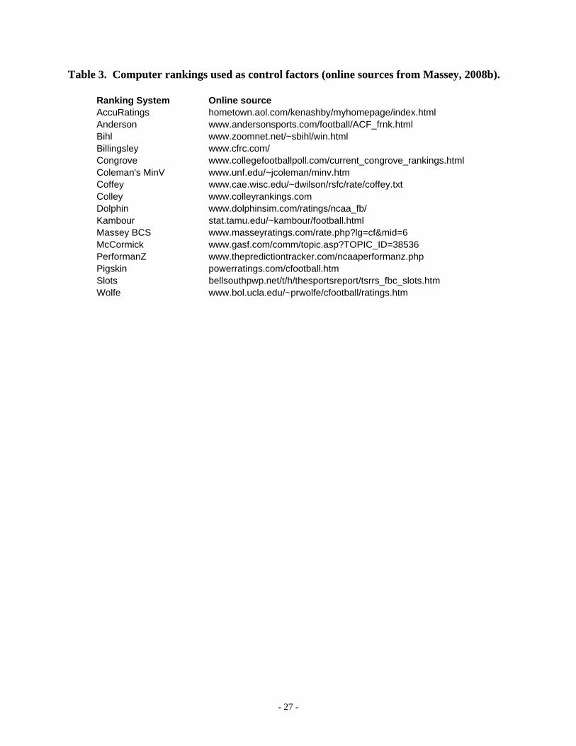
each week we collected 16 so-called computer rankings (listed in Table 3) from mratings.com,

4 Because of Notre Dame’s special status, we would have also constructed a separate binary variable for it. However, because Notre Dame did not receive any top 25 votes during any of the weeks we examined, this variable would have always carried a dependent variable (rank) value of zero in our data.

- 15 -

the web site of Kenneth Massey (2008a).5 Five of these systems – those by Massey, Anderson

and Hester, Billingsley, Colley, and Wolfe – were included as part of the BCS’s official ranking

compilation in 2007. Note that we did not include the other BCS computer ranking, from

Sagarin, as it was not included in Massey’s compilation for all weeks examined.

In addition, we sought to include other rankings that were leaders in either matching past

performance or predicting future performance, as AP voters may seek to address either or both of

these objectives (see Coleman (2005) and Stern et al. (2004) for discussion of these two

sometimes-competing goals). Coleman’s minimum violations ranking regularly represented the

best possible fit to the game results up to that point in the season (as measured by the percentage

of past games violated by the ranking). Slots was also a leading system for “retrodictive” fit

(Massey, 2008). The remaining nine systems were leading predictive systems, as compiled

week-to-week over the entire 2007 season, as compiled during the second half of the 2007

season, and/or as compiled for bowl games for 2007 and/or over the last several years.

Ashby AccuRatings, Pigskin Index, and Kambour were among the top five systems at

predicting winners over the course of the entire season (Beck, 2008). Kambour, Bihl, Ashby

AccuRatings, and Pigskin Index were in the top 10 at predicting winners during the second half

of the season (Beck, 2008). Kambour, Ashby AccuRatings, Bihl, and Congrove were in the top

four (including ties) at predicting the post-season bowl game winners in 2007 (Beck, 2008).

According to Trono (2008), McCormick, Dolphin, Coffey, and Kambour were the top four

systems at predicting bowl game winners collectively over the six seasons from 2002 through

2007, and PerformanZ was sixth in that group.

5 Since these rankings only covered the 120 FBS teams, Appalachian State and Northern Iowa were each assigned a ranking of 121 in all computer rankings. In addition, some systems did not include Western Kentucky (WKU) due to its probationary FBS status. In such cases, we assigned WKU the 120th position in that system’s ranking.

- 16 -

Because of the strength of these systems at matching past and/or future game results,

and/or (in the case of the BCS systems) because of their high profile, they were viewed as

effective controls for our analysis. For each week, we computed the mean ranking from these 16

models, and used the resulting mean as our control variable for team performance.

The data collection and variable construction process generated 28 independent variables:

27 bias factors and one control factor. In order to alleviate concerns that factors associated with

the number of losses and previous TV exposure were monotonically non-decreasing over time,

we standardized all the non-binary variable values within a given week by converting each to a

z-score. This adjustment also allowed us to compare variable coefficients more directly to

determine which factors had the strongest relationship to voter rankings.

IV. Methodology

When determining his/her ranking of the top 25 teams each week, a voter is assumed to

assess the performance merits (and/or those team characteristics outlined in the previous section)

of all available teams in a given week. However, the observed ranking for a given voter reflects

only the ordinal realization of that voter’s otherwise latent rating for each team that week, and

then only for the top 25 teams in that voter’s latent rating. Thus, our data set of 71,370

observations can be viewed as a censored one, in which the team value (the ranking) is censored

to a value of zero for all teams ranked 26 through 121 by a given voter in a given week.

Moreover, given that the ranking is an ordinal representation of the underlying rating, we only

observe a voter’s order for the teams s/he ranks, and not necessarily the distance between or

among teams in his/her latent rating.6

6 See Goff (1996) for a similar discussion of data characteristics encountered in modeling the AP poll.

- 17 -

Our dependent variable is the (reverse-scored) rank assigned to each team by the voter

(and equal to zero for any team not included in the voter’s top 25 for that week). Therefore, we

identified cumulative logit, cumulative probit, or censored tobit models as potentially appropriate

approaches to estimate parameters. Using SAS Version 9.1 (SAS, 2004), a cumulative logit

model including all of our independent variables converged. However, the null hypothesis of the

score test for the proportional odds assumption was rejected with a p-value of 0.0001, thereby

invalidating that approach. Similarly, a cumulative probit model converged, but with warnings

regarding model fit (it also failed the score test for the equal slopes assumption with a p-value of

0.0001). However, a censored tobit model did successfully converge, and it is the result of that

estimation that we report here.7

However, in order to investigate more thoroughly the impact of various groups of factors,

we report three versions of the censored tobit. Model 1 included all factors. Model 2 included

all team and bias factors, but omitted our control variable (the mean computer ranking). Model 3

included only the TV factors. This final model allowed us to investigate the degree to which the

poll simply mirrors TV coverage.

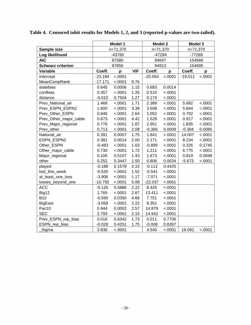
V. Results The results for all three models are shown in Table 4. The fit of our primary model

(Model 1) was good, as the log likelihood of -43,760 was substantially lower than the log

likelihood of -87,062 that would have been achieved by fitting an intercept-only model. It was

also lower than the log likelihood generated from a model including only our control variable

(log likelihood = -49,218), implying that our bias factors collectively contributed to model

7 Although the cumulative logit failed the proportional odds test, its results were quite similar to those for the censored tobit.

- 18 -

strength. Model 1’s AIC and Schwarz criterion values were also substantially improved over the

174,129 and 174,147 values yielded (respectively) by an intercept-only model.

All the Model 1 goodness-of-fit measures were also superior to those of Model 2,

meaning that our control variable contributed substantively to model fit. A comparison of the

fits of Models 2 and 3 indicates that voter ballots certainly do not simply track television

coverage. Model 3, containing only the TV factors, exhibited relatively poor log likelihood (-

77,269), AIC (154,566), and Schwarz criterion (154,695) values when compared to Models 1

and 2, and these goodness-of-fit metrics were not that dramatically improved over those for an

intercept-only model. The log likelihood was also much worse than the log likelihood from a

model including only the control variable (-49,218).

Table 4 also contains variance inflation factors (VIFs) for Model 1, computed from an

ordinary least squares fit of the model. Our control variable exhibits a relatively high VIF, which

was expected given its nature as a control. However, in no case does it appear that collinearity

substantially impacted the variances of the bias factors tested here nor the findings reported

below.

In terms of our control factor, Model 1 indicates that the mean computer ranking is

statistically significantly related in the expected direction to the placement of a team on an AP

voter’s ballot, with a p-value less than 0.0001.8 Moreover, the coefficient of this factor was

easily the largest in the model. These results suggest that AP votes are indeed highly related to

the computer rankings, and lend credence to our selection of the included rankings as controls.

In terms of our research questions regarding bias, we find that the results for Model 1

offer support for several of our hypothesized biases. Voters appear to favor teams located in

8 Note that the computer rankings were not reverse-coded, meaning that a higher ranking value represents a worse ranking, and implies that the coefficient was expected to be negative.

- 19 -

their home states, as this factor was significant at the 0.001 level. Geographic bias also extended

to teams with fellow conference members in the same state as the voter, with a p-value less than

0.0001. As might be expected, the coefficient of bias toward local conferences was smaller than

the coefficient of bias toward local teams. However, the coefficient for the distance factor was

not significant, implying that teams that are more geographically remote from the voter do not

receive less consideration than those that are located more closely.9 The collective results for the

three regional bias factors suggest that voter bias appears to be state-related and not distance-

related.

Teams appearing on television also received benefit from voters, although it was the

cumulative effect of prior appearances that was typically more highly related to receiving AP

poll votes than was an appearance in the current week. The coefficient of the previous number

of appearances was statistically significant at the 0.0001 level in Model 1 for all six network

types. Moreover, the relative coefficient sizes were generally as expected, with appearances on

the national networks and the major ESPN outlets receiving the greater weights. In regard to

appearances in the most recent week, only teams playing on the other ESPN outlets, the major

regional networks, and the non-delineated (“other”) networks received insignificant weights

(under a hypothesis that each should be positive). Again, this is not surprising, given the lower

overall exposure – and less prestige – associated with these outlets vis-à-vis the national

networks and the prominent cable networks.

In regard to bias associated with playing and performance in the most recent week, teams

that played in the most recent week were not more likely to receive greater consideration from

voters, implying no overt penalty for teams during a bye week. However, losing in the most

9 The coefficient of distance was hypothesized to be negative, given that higher distances of teams from voters were expected to yield lower rankings.

- 20 -

recent week was adversely treated by voters (over and above the cumulative number of losses for

the team over the course of the season to that point).10 This finding should come as no surprise

to those who even casually follow college football, given the dearth of teams that seem to remain

near their previous ranking immediately after a loss.

The statistically significant coefficients for the two variables reflecting the cumulative

number of losses appear consistent with the findings of Lebovic and Sigelman (2001) and Paul et

al. (2007), and suggest that voters have a bias toward one of the most simplistic performance

metrics available. The absolute value of the coefficient for having at least one loss was the third

largest among all those in Model 1 (and significant at the 0.0001 level), and the effect was

magnified even further for those losses beyond one. (Only the coefficient of our control variable

surpassed the coefficients of these two factors.) Clearly, voters seem to factor in the number of

losses when casting top 25 ballots. These findings are particularly notable given that our model

already controls for team performance with the mean of numerous computer rankings that are

much more complex and comprehensive metrics than the simple number of losses.

We also find evidence of bias in top 25 balloting favoring three of the six BCS

conferences, with only the ACC appearing to be treated similarly to non-BCS schools. The Big

East and Big 10 actually received a statistically worse treatment than non-BCS teams. There is

little support for the notion of an East Coast bias as it pertains to the Pac-10, which actually

received statistically significant favor from voters – albeit with a coefficient that was less than

those for the Big 12 and SEC, which each received inordinately strong consideration also. This

finding implies that favorable voter bias was attributed to conferences from the eastern, central,

and western portions of the country.

10 Stated otherwise, a loss in the most recent week was treated more harshly than losses earlier in the season.

- 21 -

Relative to the Big East, even a casual college football spectator is likely to perceive the

Big East as more of a basketball than football conference, with teams such as the University of

South Florida, Rutgers University, and the University of Connecticut that are relative newcomers

to the national football consciousness. Thus, that finding is not necessarily surprising. The

national perception of the ACC might be argued to be similar in regard to its historically higher

emphasis and success in basketball, which may have contributed to its insignificant coefficient

vis-à-vis non-BCS teams. The Big 10’s significant and negative coefficient may be a result of the

relatively poor performances by historical stalwarts Ohio State University in the preceding

season’s national championship game, and the University of Michigan in the 2007 season

opener. Michigan, which entered the game ranked #5 in the AP poll, lost at home to FCS

member Appalachian State University. It thereby became the highest-ranked FBS member ever

to lose to a team from the lower division, and subsequently experienced the largest drop ever in

the history of the AP poll (ESPN.com, 2007).11

Finally, neither of our variables representing bias by the three ESPN-affiliated voters

were significant in Model 1. This suggests that these voters do not show favor toward teams

playing on the group of ESPN networks, over and above any of the other biases summarized

above that might be shared with other AP poll voters.

Model 2, which included all of our bias factors but omitted our control variable,

generated findings that were largely very consistent with those from Model 1. Even in the

absence of the control, Model 2 still suggested that voting behavior exhibited state-oriented

regional bias as well as TV-related bias. In addition, and like Model 1, the Model 2 results

11 A similar observation might be made for the ACC, where historically prominent members Florida State University and the University of Miami have struggled by comparison in recent years.

- 22 -

showed highly significant coefficients for the three variables representing the number and

recency of losses.

Given the much larger (and highly significant) coefficients for all the BCS conferences in

Model 2 vis-à-vis Model 1, it appears that these binary bias variables served additionally as

partial proxies for the missing control variable in Model 2. Moreover, the much larger Model 2

coefficients for the two variables reflecting the number of losses implies that these factors also

helped to serve as a further partial proxy for team performance in that model.

VI. Conclusion

Our research confirms numerous hypothesized biases by Associated Press college

football poll voters. Voter ballots exhibit bias toward teams and conferences represented in their

home states, toward three of the six Bowl Championship Series conferences, toward teams that

accumulate higher numbers of prior television appearances, and toward teams that played on

relatively prominent TV networks in the current week. Our analysis also indicates that voters are

biased toward arguably the most simplistic performance measure available – the number of

losses – and inordinately punish teams accordingly in their ranking. All of the above has

significant managerial ramifications on the selection and distribution of voters by the Associated

Press, and whether the champions so designated would have been the same without such bias.

To the extent that similar biases may have existed in prior seasons, it also calls into question the

BCS’s previous use of the AP poll in its determination of its national champion.

- 23 -

Table 1. Associated Press college football poll voters for 2007 (AP college poll voters, 2008b).

State Voter Affiliation Alabama Neal McCready Mobile Press-Register Alabama Jay G. Tate Montgomery Advertiser Arizona John Moredich Tucson Citizen Arkansas Alex Abrams The Morning News of Northwest Arkansas California Kevin Pearson Riverside Press-Enterprise California Ray Ratto San Francisco Chronicle California Scott Wolf Los Angeles Daily News California Jon Wilner San Jose Mercury News Colorado B.G. Brooks Rocky Mountain News Connecticut Chuck Banning The Day of New London Florida Israel Gutierrez The Miami Herald Florida David Jones Florida Today Florida Brian Landman St. Petersburg Times Georgia Adam Van Brimmer Savannah Morning News-Augusta Hawaii Paul Arnett Honolulu Star-Bulletin Idaho Mike Prater Idaho Statesman Illinois Herb Gould Chicago Sun-Times Illinois Mark Tupper Decatur Herald and Review Indiana Eric Hansen The South Bend Tribune Indiana Pete DiPrimio The Fort Wayne News-Sentinel Iowa Steve Batterson Quad City Times Kansas Tom Keegan Lawrence Journal World Kentucky Chip Cosby Lexington Herald-Leader Louisiana Glenn Guilbeau Gannett Louisiana Louisiana Scott Rabalais The Baton Rouge Advocate Maryland / DC Barker Davis Washington Times Massachusetts Steve Conroy Boston Herald Michigan David Birkett The Oakland Press Michigan John Heuser The Ann Arbor News Minnesota Chip Scoggins Star Tribune of Minneapolis Mississippi Parrish Alford Northeast Mississippi Daily Journal Missouri Mike DeArmond Kansas City Star National Chris Fowler ESPN National Craig James ABC National Stewart Mandel SI.com National Tom Hart College Sports Television Nebraska Rich Kaipust Omaha World-Herald Nevada Joe Hawk Las Vegas Review-Journal New Jersey Aditi Kinkhabwala The Bergen Record New Mexico Tommy Trujillo The New Mexican New York Rodney McKissic The Buffalo News North Carolina Dave Goren WXII-TV North Carolina Joe Giglio The News & Observer North Carolina Jim Young The News & Record of Greensboro

- 24 -

Table 1 (continued).

State Voter Affiliation Ohio Kirk Herbstreit WBNS-AM/ESPN Ohio Doug Lesmerises The Plain Dealer Ohio Matt McCoy WTVN-AM Oklahoma Myron Patton KOKH-TV Oklahoma Mike Strain Tulsa World Oregon John Hunt The Oregonian Pennsylvania Ray Fittipaldo Pittsburgh Post-Gazette Pennsylvania Anthony SanFilippo Delaware County Daily Times South Carolina Joe Person The State Tennessee Wayne Phillips The Greeneville Sun Tennessee Eric Yutzy WTVF-TV Texas Bret Bloomquist El Paso Times Texas Joseph Duarte Houston Chronicle Texas Jimmy Burch Fort Worth Star-Telegram Texas Kirk Bohls Austin American-Statesman Utah Jason Franchuk Provo Daily Herald Virginia Doug Doughty The Roanoke Times Washington Molly Yanity Seattle Post-Intelligencer West Virginia Dave Morrison The Register-Herald Wisconsin Tom Mulhern Wisconsin State Journal Wyoming Austin Ward Casper Star-Tribune

- 25 -

Table 2. Abbreviations and descriptive statistics for all variables.

All Ranked Team Observations Observations Variable Abbreviation Mean Max Mean Max Rank assigned by voter (reverse scored) rank 2.664 25 13 25

Mean computer ranking MeanCompRank 61.481 121 15.325 121 Team located in same state as voter statebias 0.030 1 0.029 1 Team's conference represented in voter's state confbias 0.171 1 0.175 1 Distance (in miles) between team and voter distance 1058.1 5394.2 1139.1 5394.2Previous # of team's games on ABC, CBS, Fox, or NBC Prev_National_air 0.741 9 1.704 8 Previous # of team's games on ESPN or ESPN2 Prev_ESPN_ESPN2 1.583 8 2.588 8 Previous # of team's games on other ESPN network Prev_Other_ESPN 2.974 14 3.210 12 Previous # of team's games on FSN, Big 10, VS, or NFL network Prev_Other_major_cable 1.156 9 1.401 6 Previous # of team's games on Lincoln Financial, Raycom, or The Mtn. network Prev_Major_regional 0.660 8 0.607 7 Previous # of team's games on other TV Prev_other 1.268 10 0.541 4 Team's game on ABC, CBS, Fox, or NBC that week National_air 0.104 1 0.290 1 Team's game on ESPN or ESPN2 that week ESPN_ESPN2 0.176 1 0.288 1 Team's game on other ESPN network that week Other_ESPN 0.201 1 0.240 1 Team's game on FSN, Big 10, VS, or NFL network that week Other_major_cable 0.079 1 0.095 1 Team's game on Lincoln Financial, Raycom, or The Mtn. network that week Major_regional 0.059 1 0.045 1 Team's game on other TV that week other 0.099 1 0.014 1

- 26 -

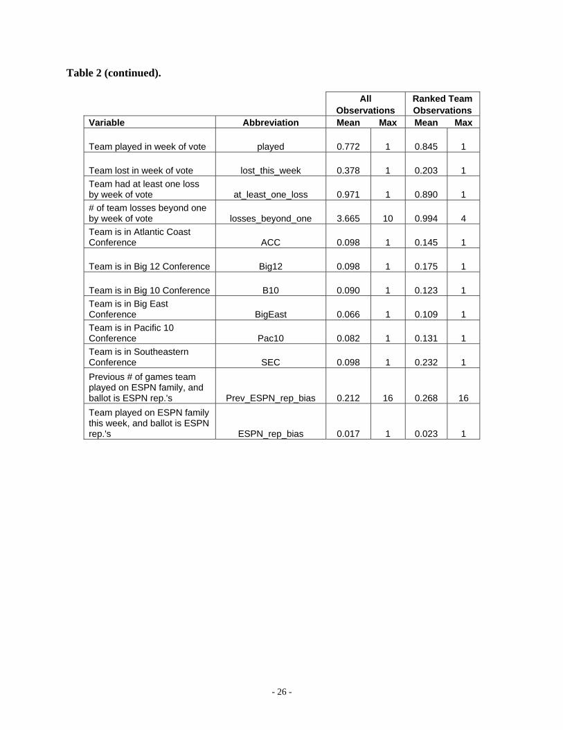
Table 2 (continued).

All Ranked Team Observations Observations Variable Abbreviation Mean Max Mean Max

Team played in week of vote played 0.772 1 0.845 1

Team lost in week of vote lost_this_week 0.378 1 0.203 1 Team had at least one loss by week of vote at_least_one_loss 0.971 1 0.890 1 # of team losses beyond one by week of vote losses_beyond_one 3.665 10 0.994 4 Team is in Atlantic Coast Conference ACC 0.098 1 0.145 1

Team is in Big 12 Conference Big12 0.098 1 0.175 1

Team is in Big 10 Conference B10 0.090 1 0.123 1 Team is in Big East Conference BigEast 0.066 1 0.109 1 Team is in Pacific 10 Conference Pac10 0.082 1 0.131 1 Team is in Southeastern Conference SEC 0.098 1 0.232 1 Previous # of games team played on ESPN family, and ballot is ESPN rep.'s Prev_ESPN_rep_bias 0.212 16 0.268 16 Team played on ESPN family this week, and ballot is ESPN rep.'s ESPN_rep_bias 0.017 1 0.023 1

- 27 -

Table 3. Computer rankings used as control factors (online sources from Massey, 2008b).

Ranking System Online source AccuRatings hometown.aol.com/kenashby/myhomepage/index.html Anderson www.andersonsports.com/football/ACF_frnk.html Bihl www.zoomnet.net/~sbihl/win.html Billingsley www.cfrc.com/ Congrove www.collegefootballpoll.com/current_congrove_rankings.html Coleman's MinV www.unf.edu/~jcoleman/minv.htm Coffey www.cae.wisc.edu/~dwilson/rsfc/rate/coffey.txt Colley www.colleyrankings.com Dolphin www.dolphinsim.com/ratings/ncaa_fb/ Kambour stat.tamu.edu/~kambour/football.html Massey BCS www.masseyratings.com/rate.php?lg=cf&mid=6 McCormick www.gasf.com/comm/topic.asp?TOPIC_ID=38536 PerformanZ www.thepredictiontracker.com/ncaaperformanz.php Pigskin powerratings.com/cfootball.htm Slots bellsouthpwp.net/t/h/thesportsreport/tsrrs_fbc_slots.htm Wolfe www.bol.ucla.edu/~prwolfe/cfootball/ratings.htm

- 28 -

Table 4. Censored tobit results for Models 1, 2, and 3 (reported p-values are two-tailed).

Model 1 Model 2 Model 3 Sample size n=71,370 n=71,370 n=71,370 Log likelihood -43760 -47294 -77269 AIC 87580 94647 154566 Schwarz criterion 87856 94913 154695 Variable Coeff. p VIF Coeff. p Coeff. p Intercept -23.184 <.0001 -25.054 <.0001 -19.511 <.0001MeanCompRank -17.171 <.0001 9.76 statebias 0.645 0.0006 1.15 0.683 0.0014 confbias 0.357 <.0001 1.26 0.515 <.0001 distance -0.010 0.7504 1.27 0.174 <.0001 Prev_National_air 1.468 <.0001 1.71 2.389 <.0001 5.682 <.0001Prev_ESPN_ESPN2 1.600 <.0001 3.39 3.508 <.0001 5.844 <.0001Prev_Other_ESPN 0.946 <.0001 2.64 1.052 <.0001 0.792 <.0001Prev_Other_major_cable 0.673 <.0001 4.42 1.528 <.0001 0.917 <.0001Prev_Major_regional 0.776 <.0001 1.87 2.951 <.0001 1.835 <.0001Prev_other 0.713 <.0001 2.08 -0.366 0.0009 -0.394 0.0080National_air 0.391 0.0007 1.75 1.841 <.0001 14.007 <.0001ESPN_ESPN2 0.381 0.0014 2.00 2.171 <.0001 8.234 <.0001Other_ESPN -0.483 <.0001 1.63 -0.895 <.0001 0.326 0.1745Other_major_cable 0.730 <.0001 1.72 1.211 <.0001 6.775 <.0001Major_regional 0.105 0.5107 1.43 1.673 <.0001 0.819 0.0699other 0.252 0.3447 1.50 0.806 0.0034 -5.673 <.0001played -0.188 0.1578 2.15 -0.112 0.4425 lost_this_week -0.535 <.0001 1.52 -0.541 <.0001 at_least_one_loss -3.906 <.0001 1.17 -7.071 <.0001 losses_beyond_one -10.792 <.0001 5.08 -22.037 <.0001 ACC -0.126 0.5886 2.22 8.425 <.0001 Big12 1.765 <.0001 2.67 13.411 <.0001 B10 -0.590 0.0350 4.66 7.751 <.0001 BigEast -3.058 <.0001 2.22 8.351 <.0001 Pac10 0.944 0.0002 2.57 14.879 <.0001 SEC 2.793 <.0001 2.15 14.942 <.0001 Prev_ESPN_rep_bias 0.016 0.6342 1.73 0.011 0.7706 ESPN_rep_bias -0.028 0.4251 1.75 -0.008 0.8397 _Sigma 3.836 <.0001 4.540 <.0001 16.091 <.0001

- 29 -

References

AP College Poll Voters (2007). Retrieved weekly between October 19, 2007 and December 7,

2007 from

http://hosted.ap.org/dynamic/files/specials/collegefootball_front/votes/voters.html?SITE=

AP&SECTION=HOME.

AP College Poll Voters (2008a). Retrieved on January 16, 2008 from

http://hosted.ap.org/dynamic/files/specials/collegefootball_front/votes/voters.html?SITE=

AP&SECTION=HOME.

AP College Poll Voters (2008b). Retrieved on June 10, 2008 from

http://hosted.ap.org/dynamic/files/specials/collegefootball_front/votes/voters.html?SITE=

AP&SECTION=HOME.

Beck, T. (2008). Computer rating system prediction results for college football (NCAA IA).

Retrieved on June 10, 2008 from

http://www.thepredictiontracker.com/ncaaresults.php?type=1&orderby=

wpct%20desc&year=07.

Callaghan, T., Mucha, P.J., & Porter, M.A. (2004). The Bowl Championship Series: A

mathematical review. Notices of the AMS, 51(8), 887-893.

Campbell, N.D., Rogers, T., & Finney, R.Z. (2007). Evidence of television exposure effects in

AP top 25 college football rankings. Journal of Sports Economics, 8(4), 425-434.

Carey, J., & Whiteside, K. (2004). AP drops poll from BCS mix. USA Today. Retrieved on June

26, 2008 from www.usatoday.com/sports/college/football/2004-12-21-ap-bcs-

withdrawal_x.htm.

- 30 -

College Football Weekly TV Schedules (2008). Retrieved on June 7, 2008 from

mattsarz44017.tripod.com/football2007.html.

Donahue, K. (2005). AP sends out poll voting suggestions. Retrieved on July 22, 2008 from

www.fanblogs.com/ap_poll/005412.php.

ESPN.com (2007). Ducks win, now prepare for embarrassed Michigan. Retrieved on July 21,

2008 from http://sports.espn.go.com/ncf/preview?gameId=272510130.

Goff, B. (1996). An assessment of path dependence in collective decisions: Evidence from

football polls. Applied Economics, 28, 291-297.

Lebovic, J.H., & Sigelman, L. (2001). The forecasting accuracy and determinants of football

rankings. International Journal of Forecasting, 17, 105-120.

Logan, T.D. (2007). Whoa, Nellie! Empirical tests of college football's conventional wisdom.

NBER Working Papers 13596, National Bureau of Economic Research, Inc. Retrieved

on July 24, 2008 from www.econ.ohio-state.edu/trevon/w13596.pdf.

Longman, J. (2002). On college football; Miami drop an indictment of the polls. Retrieved on

July 22, 2008 from

query.nytimes.com/gst/fullpage.html?res=9A00E7DF103EF935A35752C1A9649C8B63.

Massey, K. (2008a). College football ranking comparison. Retrieved on March 7, 2008 from

www.mratings.com/cf/compare.htm.

Massey, K. (2008b). Retrieved on March 7, 2008 from www.mratings.com/cf/compare.csv.

Miller, T. (2001). Stamping out bias. Retrieved on July 22, 2008 from

sportsillustrated.cnn.com/football/college/2001/preview/pac10_feature/.

NCAA (2008). Retrieved on June 26, 2008 from www.ncaa.com/football/default.aspx?id=216.

- 31 -

Paul, R.J., Weinbach, A.P., & Coate, P. (2007). Expectations and voting in the NCAA football

polls: The wisdom of point spread markets. Journal of Sports Economics, 8(4), 412-24.

Reinardy, S. (2004). No cheering in the press box: A study of intergroup bias and sports

writers.” Retrieved on June 26, 2008 from

apse.dallasnews.com/news/2004/biasinsportsreporting.pdf.

SAS Version 9.1, (2004), SAS Institute, Inc., Cary, North Carolina.

Shanoff, D. (2006). AP top 25 individual ballot analysis. Retrieved on July 22, 2008 from

www.danshanoff.com/2006/10/ap-top-25-individual-ballot-analysis.html.

Steinberg, D. (2006). On treacherous AP voters.” Retrieved on July 22, 2008 from

blog.washingtonpost.com/dcsportsbog/2006/10/on_treacherous_ap_voters.html.

Stern, H.S., Massey, K., Harville, D.A., Billingsley, R., et al. (2004). Statistics and the college

football championship / discussion / reply.” The American Statistician, 58(3), 179-195.

Trono, J. (2008). Overtake and feedback ranking system page.” Retrieved on March 7, 2008

from academics.smcvt.edu/jtrono/OAF.html.

Tsai, Y-M., & Sigelman, L. (1980). Stratification and mobility in big-time college football.

Sociological Methods and Research, 8, 487-497.