volume rendering - classesclasses.engr.oregonstate.edu/eecs/spring2010/cs551/lectures/vol... · •...
TRANSCRIPT

4/20/2010
1
Volume Rendering
Concept and techniques
Contents
• Introduction– Volume dataset
l• A voxel• Examples
– How is different from a surface based dataset?
• Volume rendering ‐ Concept– The transfer function– Gradient vector
• Techniques– Surface extraction– Ray tracing– Footprint evaluation– Texture mapping
• Conclusion

4/20/2010
2
Introduction (1/4)
• Volume Data– A volume is a 3‐D array of voxels.y
• Notion of a voxel
– A volume dataset is 3‐D array of voxels with a scalar or vector field (possibly other type of fields).
Introduction (2/4)
• Volume Data
– A volume dataset is a 3‐D array of voxels.
• Notion of a voxel
– A volume dataset is 3‐D array of voxels with a scalar or vector field (possibly other type of fields).
• Significance
–Where does it come from?
• Medical imaging – CT scan, MRI, etc.
• Simulations – Fluid simulation, molecular physics, etc.
– How is it different from a surface based dataset?
–Why is it important?

4/20/2010
3
An example of volume rendering
Courtesy : Visualization group, Lawrence Berkeley National Laboratory.
Introduction (3/4)
• Volume Data
– A volume dataset is a 3‐D array of voxels.
• Notion of a voxel
– A volume dataset is 3‐D array of voxels with a scalar or vector field (possibly other type of fields).
• Significance
– Where does it come from?
• Medical imaging – CT scan, MRI, etc.
• Simulations – Fluid simulation, molecular physics, etc.
– How is it different from a surface based dataset?
–Why is it important?

4/20/2010
4
Introduction (4/4)
• Volume Data
– A volume dataset is a 3‐D array of voxels.
• Notion of a voxel
– A volume dataset is 3‐D array of voxels with a scalar or vector field (possibly other type of fields).
• Significance
– Where does it come from?
• Medical imaging – CT scan, MRI, etc.
• Simulations – Fluid simulation, molecular physics, etc.
– How is it different from a surface based dataset?
Wh i it i t t?– Why is it important?
• Volume rendering
– Rendering a volume dataset into 2‐D image plane.
Volume Rendering – Concept (1/9)
• Let us denote scalar function for a voxel ( , , )i j kx y z( )fas .
• Transfer function
– A map from scalar values to color and opacity.
( , , )i j kf x y z
: ( , , ) ( , , ), ( , , )i j k i j k i j kT f x y z C x y z x y z

4/20/2010
5
Volume Rendering – Concept (2/9)
• Transfer function– A map from scalar values to color and opacity.p p y
– An example
: ( , , ) ( , , ), ( , , )i j k i j k i j kT f x y z C x y z x y z
Volume Rendering – Concept (3/9)
• Gradient
The direction of greatest rate of change– The direction of greatest rate of change.
– Can be approximated for every voxel numerically.
1 1 1 1
1 1
1 1( , , ) ( , , ) , ( , , ) ( , , ) ,
2 2( , , )1
( , , ) ( , , )2
i j k i j k i j k i j k
i j k
i j k i j k
f x y z f x y z f x y z f x y zf x y z
f x y z f x y z

4/20/2010
6
Volume Rendering – Concept (4/9)
• Rendering modelData corrections,
Raw data
Data ( , , )i j kf x y z
Voxel Color Voxel Opacity
,noise removal, etc.
Shading Classification
( , , )i j kC x y z ( , , )i j kx y z
2‐D Image
Rendering (Ray‐tracing, Footprintevaluation,Texture mapping, etc.
Volume Rendering – Concept (5/9)
• Shading
– A part of transfer function.
– Determines RGB color components for a voxel.
• Based on – Gradient direction
– Lighting condition
– Material reflectivityMaterial reflectivity
– Distance from image plane
4/20/2010
7
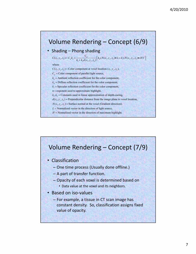
Volume Rendering – Concept (6/9)• Shading – Phong shading
( , , ) ( ( , , ) ( ( , , ) )( )p n
i j k p a d i j k s i j k
CC x y z C k k N x y z L k N x y z H
k k d x y z 1 2 ( , , )
where
( , , ) Color component at voxel location ( , , ),
Color component of parallel light source,
Ambient reflectio
j p j ji j k
i j k i j k
p
a
k k d x y z
C x y z x y z
C
k
n coefficient for the color component,
Diffuse reflection coefficient for the color component,
Specular reflection coefficient for the color component,d
s
k
k
1
exponent used to approximate highlight,
,
n
k k
2 Constants used in linear approximation of depth-cueing,
( , , ) Perpendicular distance from the image plane to voxel location,
( , , ) Surface normal at the voxel (Gradient direction).
Normal
i j k
i j k
d x y z
N x y z
L
ized vector in the direction of light source,
Normalized vector in the direction of maximum highlight.H
Volume Rendering – Concept (7/9)
• Classification
– One time process (Usually done offline.)
– A part of transfer function.
– Opacity of each voxel is determined based on
• Data value at the voxel and its neighbors.
• Based on iso‐valuesBased on iso values
– For example, a tissue in CT scan image has constant density. So, classification assigns fixed value of opacity.

4/20/2010
8
Volume Rendering – Concept (8/9)• Classification
– User defined lookup table
• Scalar value vs. Opacity.
– For each scalar value a band of voxels is assigned opacity and rest are kept transparent.
( , , ) if ( , , ) 0
and ( , , )
( , , )1( , , ) 1
(
i j k v i j k
i j k v
v i j ki j k v
x y z a f x y z
f x y z f
f f x y zx y z a
r f
if ( , , ) 0 and
, , )i j k
i j k
f x y zx y z
( , , ) ( , , )
i j k i j k vf x y z r f x y z f
( , , ) ( , , ) ,
( , , ) 0 otherwise.
Where,
is the iso-value for which opacity is being assigned.
is assigned opacit
i j k i j k
i j k
v
v
f x y z r f x y z
x y z
f
y value from lookup table.
Volume Rendering – Concept (9/9)
• Classification
– Opacities for different iso‐values are composited to obtain final opacities.
Given, selected values of scalar function , where 1 ,
corresponding opacities, and region thickness , we can compute
opacities ( ) using previous equation
n
n
v
v n
f n N
r
x y z
opacities ( , , ) using previous equation.
1( , , ) 1 (1
n i j kx y z
N
tot i j k nx y z
( , , )).n i j kx y z

4/20/2010
9
Volume Rendering – Techniques (1/6)
• Rendering model – Ray‐tracingeyeeye
Image pixel with color C
Viewing ray Sample points
A voxel with color and opacity
( , , )i j kC x y z
( , , )i j kx y z
Volume Rendering ‐ Techniques (2/6)
• Rendering model – Ray‐tracingData ( )fData ( , , )i j kf x y z
Voxel color( , , )i j kC x y z
Voxel opacity( , , )i j kx y z
ShadingClassification
Sample color Sample opacity( )C s ( )s
Ray‐tracing/ Re‐sampling
2‐D Image Pixel color
( ) ( )
Compositing
( , )outC i j

4/20/2010
10
Volume Rendering – Techniques (3/6)
• Compositing
– Back to front order
– Using transparency formula
Given, Color of the ray as it enters a sample point s, ( , ),
Color and opacity at sample point,
( ) & ( ) respectively, Color of output ray is given by
( , ) ( , ) 1 ( ) ( ) ( ).
in
out in
C i j
C s s
C i j C i j s C s s
( , ) ( , ) ( ) ( ) ( )out inj j
Results with ray‐tracing

4/20/2010
11
Volume Rendering – Techniques (4/6)
• Footprint evaluation
– Each voxel is splattered on image plane.
• Projected is not an accurate term for this.(why?)
Splat!
Courtesy – Westover et. al.
Volume Rendering – Techniques (5/6)
?
Ray tracing Splattering
Courtesy – Westover et. al.

4/20/2010
12
Volume Rendering – Techniques (6/6)
• Footprint evaluation
– Footprint of a voxel is determined by a Gaussian distribution function.
– Footprint changes according to distance of voxel from image plane.
– Preprocessing.
• Compositing
Thank you!