Volume preserving CES and CET formulations

Dominique van der Mensbrugghe and Jeffrey C. Peters∗

The Center for Global Trade Analysis, Purdue University

June 5, 2016

Abstract

Two of the most widely used functional forms in quantitative economic analysis are theconstant-elasticity-of-substitution (CES) and constant-elasticity-of-transformation (CET) func-tions. The CES functional form is oft-used to represent production functions—for example, inmacro growth models or in multi-sector CGE models—or preference functions—for example theArmington specification for allocating domestic absorption across purchases of domestic andimported goods. In other contexts, the CET functional form is used to allocate production orsupply across different markets—for example to allocate domestic production between domesticand export markets or to allocate land supply across various land uses.

As the CES and CET specifications are now increasingly implemented in broader contexts,notably with economic models integrating more and more engineering and bio-physical prop-erties, one potential drawback of their use is that they do not preserve additivity, i.e. thesum of the volume components do not add up to the total volume. In the case of land-use,for example, the sum of hectares devoted to different crops do not necessarily add up to totalcrop-land. The volume discrepancies can potentially be small and ’adjusted’ away, though apaper by Fujimori et al. (2014) suggest that in the case of long-term land-use allocation, thediscrepancies can become quite large, particularly at the more (spatially) disaggregated level.Even if the volume discrepancies are small, deviations from strict additivity are often confusingto scientific colleagues from other disciplines.

This paper explores the use of a modified CES/CET function that has virtually the sameattributes of the standard CES/CET function but preserves additivity. The additive formof the CET has been introduced in labor allocation decisions by Dixon and Rimmer (2003)and Dixon and Rimmer (2006) and land-use allocation by Giesecke et al. (2013). This paperprovides the analytical formulation of both the standard and additive forms of the CES/CETfunction. It compares the implementation of the additive CET using a small numerical exampleto highlight some key potential differences between the two formulations and then introducesthe additive form of the CET function in the land-use allocation module of the Envisage Modeland assesses the impacts of the two formulations on agricultural output, prices and land-use ina long-term global scenario.

1 Introduction

Two of the most widely used functional forms in quantitative economic analysis are the constant-elasticity-of-substitution (CES) and constant-elasticity-of-transformation (CET) functions. TheCES functional form is oft-used to represent production functions—for example, in macro growth

∗Paper being presented at the 19th Annual Conference on Global Economic Analysis, The World Bank, Washing-ton, DC, June 15-17, 2016. The authors would like to acknowledge useful discussions with Peter Dixon and ThomasHertel. Correspondence should be sent to Dominique van der Mensbrugghe (vandermd@purdue.edu).

1

models or in multi-sector CGE models—or preference functions—for example the Armington spec-ification for allocating domestic absorption across purchases of domestic and imported goods. Inother contexts, the CET functional form is used to allocate production or supply across differentmarkets—for example to allocate domestic production between domestic and export markets or toallocate land supply across various land uses.

As the CES and CET specifications are now increasingly implemented in broader contexts,notably with economic models integrating more and more engineering and bio-physical properties,one potential drawback of their use is that they do not preserve additivity, i.e. the sum of thevolume components do not add up to the total volume.1 In the case of land-use, for example, thesum of hectares devoted to different crops do not necessarily add up to total crop-land. The volumediscrepancies can potentially be small and ’adjusted’ away, though a paper by Fujimori et al. (2014)suggest that in the case of long-term land-use allocation, the discrepancies can become quite large,particularly at the more (spatially) disaggregated level. Even if the volume discrepancies are small,deviations from strict additivity are often confusing to scientific colleagues from other disciplines.2

One of the key alternatives to the CES/CET functions has been the use of the logit specifi-cation, see for example Edmonds and Reilly (1985), Kyle et al. (2011) and Fujimori et al. (2014).Edmonds and Reilly (1985) use the logit to determine market shares of various energy technologies.Kyle et al. (2011) and Fujimori et al. (2014) use the logit to determine the allocation of land acrossuses. One clear advantage of the logit specification is the preservation of volume additivity. Thepaper by Fujimori et al. (2014) compares the use of the logit and CET specifications for allocatingland in the AIM CGE model.

In this paper we introduce an alternative to the standard CES/CET specification, which we willcall the additive CES/CET specification, or ACES/ACET. Examples of this specification come fromDixon and Rimmer (2006) and Giesecke et al. (2013). The former paper uses the additive CET toallocate the supply of workers (in a given category) across different activities, including the decisionto be unemployed. The sum across all activities (including unemployment) sums to the total laborsupply. The paper by Giesecke et al. (2013) uses the additive CET for land-use allocation.

The first two sections focus on the analytical properties of the standard CES/CET specificationand its additive variant. Subsequently, a small numerical example of land-use is used to elucidatesome of the key differences between the two specifications and under what conditions the two couldlead to significantly different responses to shocks. The additive specification is then incorporatedin the Envisage model that is a global recursive dynamic computable general equilibrium (CGE)model. The model has been used to derive projections for food and agriculture through 2050 in thecontext of the so-called Share Socio-Economic Pathways (SSPs). Impacts in 2050 on agriculturaloutput, prices and land-use are compared across the two different CET specifications for landallocation.

2 The standard CET/CES formulas

2.1 The CET specification

We start with describing the CET specification—even if the CES is more widely used for nestedproduction structures and/or utility/sub-utility specifications (for example the ubiquitous Arming-

1 In many contexts the notion of additivity is not relevant, for example in the case of CES bundle composed ofcapital and labor. Additivity is clearly relevant when the components of the CES/CET are being measured inidentical units.

2 Bowles (1970) explored the deviations from additivity in the context of labor demand across different skill types.He concludes that the discrepancies, in this case, is not particularly large.

2

ton assumption in specifying import demand). However, the most widely used applications to dateof the volume preserving CET/CES specifications are on the supply side.3 Dixon and Rimmer(2003) and Dixon and Rimmer (2006) introduce the additive form of the CET to allocate laborsupply decisions across multiple activities (including unemployment). And in a different contextGiesecke et al. (2013) introduce the same functional form to allocate land supply across multipleuses. This harks back to the above-cited references to land-use specification using the logit functionthat also has the additive property.

The standard CET function is often used to allocate supply of a good across different desti-nations so as to maximize total revenue. It is used for example to allocate land supply acrossdifferent potential uses and to allocate domestic production across destination markets—domesticand foreign—analogously to the use of the CES to determine commodity demand by region of origin(the Armington assumption). The basic setup is given by equation (1)—the revenue function tomaximize, subject to equation (2) that represents the transformability across markets.

maxXi

∑

i

PiXi (1)

subject to

V = A

[

∑

i

gi (λiXi)ν

]1/ν

(2)

where V is the aggregate volume (e.g. aggregate supply), Xi are the relevant components (market-specific supply), Pi are the corresponding prices, gi are the CET (primal) share parameters, and νis the CET exponent. The parameters A and λi are shifters that can be used to implement changesin preferences or technology, where A is a global shifter, for example an overall decrease or increasein ’quality’ adjusted supply of land, and the λ parameters are changes that are component specific,for example a preference shift to supplying a specific type of land. The CET exponent is relatedto the CET transformation elasticity, ω via the following relation:

ν =ω + 1

ω⇔ ω =

1

ν − 1

The transformation elasticity is assumed to be positive. Solution of this maximization problemleads to the following first order conditions:

Xi = γi (Aλi)−1−ω

(

Pi

P

)ω

V (3)

and

P =1

A

[

∑

i

γi

(

Pi

λi

)1+ω]1/(1+ω)

(4)

where the γi parameters are related to the primal share parameters, gi, by the following formula:

γi = g−ωi ⇔ gi =

(

1

γi

)1/ω

3 Peters (2016) introduces the additive CES in determining power demand from various sources—thermal, nuclear,hydro, etc.

3

The interpretation of equation (3) is that supply to market i is a share of aggregate supply, V ,where the share depends positively on the market price in market i relative to the aggregate price(given by P ). The price sensitive part of the market share depends on the degree of transformabilityacross markets, i.e. on ω. In one extreme case, when ω is 0, the shares are fixed. In the otherextreme case, when ω is infinite, allocation is based on perfect mobility (i.e. perfect homogeneity)and the law-of-one-price must hold: Pi = P .4

Note that the resulting formulas only depend on the dual share parameters (γi) and the trans-formation elasticity. Hence, the implementation of the CET does not require the primal parametersincluding the exponent. Calibration is straightforward given initial values for P , V , Pi, Xi and thetransformation elasticity ω and assuming the technology (or preference) parameters are initializedat unit values. We have:

γi =Xi

V

(

P

Pi

)ω

If initial prices are all equal, then the dual revenue share parameters, si, are equal to the base yearvalue shares, i.e.:

si =PiXi

P.V= γi

In the case of the CET, it can be shown that the aggregate price index, calculated from equa-tion (4), is the same as the aggregate price calculated from the zero profit condition, i.e.:

P.V =∑

i

PiXi

As we will see below, this condition does not hold in the case of the additive CET. It is alsoeasy to show that P is equal to the shadow price of the Lagrangian function.

If we log-differentiate the two expressions above, we can derive a convenient intuitive interpre-tation of the CET formulas.5 The log-differentiated forms are given by, where a dot over a variablerepresents percentage change of the variable in levels:

∂Xi

Xi=

.Xi =

.V + ω

( .Pi −

.P)

− (1 + ω)( .λi +

.A)

.P = −

.A+

∑

j

sj

[ .Pj −

.λj

]

If we substitute the second expression in the first, we have the following:

.Xi =

.V + ω

.Pi − ω

∑

j

sj

[ .Pj −

.λj

]

− (1 + ω).λi −

.A

Ignoring the technology parameters, supply to market i is the sum of three components. The first isthe scale effect, the second is the own price effect and the third reflects cross price effects. Note thatthe percent change in the aggregate price index, P , is simply the weighted average of the percentchange in the component prices (ignoring technology), where the weights are the value shares, si.This expression is independent of the transformation elasticity.

4 A more general formulation of the law-of-one-price would allow for fixed price wedges, but all prices wouldexhibit the same percentage change in case of a shock.

5 The log-differentiated forms are typical in GEMPACK implementations of CGE models.

4

2.2 The CES function

The CES function is widely used as a production function to combine Xi inputs to form a compositegood V using the so-called CES aggregation function given by equation (6).6 The producer’s (orconsumer’s) optimization problem is to minimize the the cost of inputs subject to the CES primalconstraint:

minXi

C =∑

i

PiXi (5)

subject to the constraint:

V = A

[

∑

i

ai (λiXi)ρ

]1/ρ

(6)

The price of the inputs, Pi are assumed to be given. The parameters ai are the primal shareparameters and the primal exponent, ρ, is linked to the substitution of elasticities across inputs.The parameter A is a global shifter (for example an input neutral technology shifer) and the λi

parameters are input specific shifters (or preference shifters in the case of consumer demand).There is a closed form solution to the optimization problem given by equations (7) and (8).

Equation (7) states that the demand for input i is a share of the aggregate volume V , where theshare depends negatively on the price of the input relative to the aggregate price P . The higher thesubstitution elasticity, the more the share depends on the relative price. At one extreme, with azero substitution elasticity, demand for input i is a strict proportion of the aggregate volume.7 Theaggregate price expression, equation (8), is sometimes referred to as the dual price expression. It canbe shown that the dual price expression is equivalent to the zero profit equation, i.e. P.V =

∑

i PiXi.

Xi = αi (Aλi)σ−1

(

P

Pi

)σ

V (7)

P =1

A

[

∑

i

αi

(

Pi

λi

)1−σ]1/(1−σ)

(8)

where we made the following substitutions:

σ =1

1− ρ⇔ ρ =

σ − 1

σ

andαi = a

1/(1−ρ)i = aσi ⇔ ai = α

1/σi

Similar to the derivation above for the CET, an intuitive interpretation of the CES specificationis to log-linearize the demand and aggregate price expressions. This leads to the following twoexpressions:

∂Xi

Xi=

.Xi =

.V + σ

( .P −

.Pi

)

+ (σ − 1)( .A+

.λi

)

6 It is often also used as a preference function, for example as a consumer utility or sub-utility function, forexample the Armington specification for import demand.

7 Also referrred to as a Leontief technology.

5

∂P

P=

.P = −

.A+

∑

j

sj

( .Pj −

.λj

)

Ignoring the technology terms, the change in the demand for Xi is a function of the two otherterms—the change in the aggregate volume, sometimes referred to as the scale effect, and the relativechange of the component price adjusted by the degree of substitutability, i.e. the σ parameter.

The CES is ubiquitous in CGEmodels, and, in the case of production nestings, Perroni and Rutherford(1995) and Perroni and Rutherford (1998), have shown that a nested CES production specificationcan provide the same degree of flexibility as more generic flexible functional forms. However, asmodels are now integrating more than ever physical quantities, such as energy, the one potentialdrawback of CES functions is that they don’t preserve volume additivity, i.e. V 6=

∑

iXi. Depend-ing on the nature of the simulation, the deviation from additivity may not be very significant and’adjusted’ away, but this is clearly not always the case.

The key difference between the CES and CET functions, given that both σ and ω are assumedto be positive is that the component price is in the denominator in the case of the CES function,i.e. demand goes down as the component price increases (relative to the aggregate price), whereasin the case of the CET the component price is in the numerator, i.e. supply to a given marketincreases as the price on that market increases (relative to the aggregate market price.) The CET,similar to the CES, does not preserve volume additivity. Fujimori et al. (2014) compared the use ofthe CET to the volume-preserving logit in land allocation specification and found that there weresignificant deviations to additivity in land allocation—particularly at the spatially disaggregatedlevel.

3 The additive forms of the CET/CES specification

3.1 The additive CET formulation

The additive form of the CET function starts with maximization of a utility function subjectto volume additivity. The utility function, equation (9), is a CET aggregation of the revenuesassociated with the supply to all markets. Equation (10) reflects the additivity condition.

maxU = A

[

∑

i

gi (λiPiXi)ν

]1/ν

(9)

V =∑

i

Xi (10)

The analytical solution is similar to the standard CET solution.

Xi = γi (Aλi)ω

(

Pi

P c

)ω

V (11)

P c = A

[

∑

i

γi (λiPi)ω

]1/ω

(12)

Equation (11) is the reduced form demand equation for component Xi, that, ignoring thetechnology (or preference) shifters, A and λi, is virtually identical to the standard CET expression.The one subtle difference is the price index for the composite (or aggregate) bundle, P c. This is

6

defined in equation (12). Again, ignoring the preference shifters, the price index equation differs inthat the substitution elasticity enters as ω and not as 1+ω. And in fact the composite price indexis no longer equal to the average price:

P.V =∑

i

PiXi 6= P c.V

The additive form of the CET expression requires an additional equation to find the aggregate price(i.e. the one that implements the zero profit condition) because of the non-equivalence between thecomposite price index, P c and the aggregate price defined by P . There are also differences betweenthe primal and dual parameters as described in the expressions below:

ω =ν

ν − 1⇔ ν =

ω

ω + 1

andγi = g

1/(1−ν)i = g1+ω

i ⇔ gi = γ1/(1+ω)i = γ1−ν

i

This leads to a different relationship between the transformation elasticity and the primal exponentas illustrated in Figure 1. Under the standard CET, the relationship is continuous from +∞ to 1.With the additive form, the relationship is continuous from 0 to 1. The primal exponent convergestowards 1 as the substitution elasticity increases under both forms.

Figure 1: The CET exponent (ν) as a function of the transformation elasticity

0

5

10

15

0 0.5 1.0 1.5 2.0 2.5 3.0 3.5 4.0 4.5 5.0 5.5 6.0 6.5 7.0 7.5 8.0 8.5 9.0 9.5 10.0

Transformation elasticity

CET

exponen

t

Standard

Additive

Log-differentiation of the additive CET leads to the following expressions:

.Xi =

.V + ω

( .Pi −

.

P c)

+ ω( .λi +

.A)

.

P c =.A+

∑

j

rj

[ .Pj +

.λj

]

If we substitute the second expression in the first, we have the following:

7

.Xi =

.V + ω

( .Pi +

.λi

)

− ω∑

j

rj

[ .Pj +

.λj

]

where the weights, rj , represent the volume shares, i.e.:

rj =Xj

V

Thus, a few other subtle differences are that the percentage change in the composite price index usesthe volume weights and not the value weights as in the standard CET and the technology/preferenceshifters have a positive impact on supply and the composite price index—not a negative impact.We can also show that the following relationship holds:

λ = u/V = P c

where λ is the Lagrange multiplier. Since u is an ordinal concept, we have an extra degree offreedom in calibration. One could initialize P c to the aggregate price (P ) and then calculate uusing the expression above.

3.2 The additive CES formulation

The additive form of the CES function minimizes the utility that is a CES aggregation of the costsof the components and not the usual CES aggregation of the components themselves. Hence weminimize equation (13) subject to the additivity constraint, i.e. equation (10):

minU = A

[

∑

i

ai (λiPiXi)ρ

]1/ρ

(13)

We can derive the following solution:

Xi = αi (Aλi)−σ

(

P c

Pi

)σ

V (14)

P c = A

[

∑

i

αi (λiPi)−σ

]

−1/σ

(15)

Equation (14) is the reduced form demand equation for component Xi, that, ignoring thetechnology (or preference) shifters, A and λi, is virtually identical to the standard CES expression.As in the case of the additive CET, the price index for the composite (or aggregate) bundle, P c,is no longer equal to the average price, P , and the substitution elasticity enters as −σ and not as1− σ.

There are also differences between the primal and dual parameters as described in the expres-sions below:

σ =ρ

ρ− 1⇔ ρ =

σ

σ − 1

andαi = a

1/(1−ρ)i = a1−σ

i ⇔ ai = α1/(1−σ)i = α1−ρ

i

This leads to a different relationship between the substitution elasticity and the primal exponentas illustrated in Figure 2. Under the standard CES, the relationship is continuous from −∞ to 1.

8

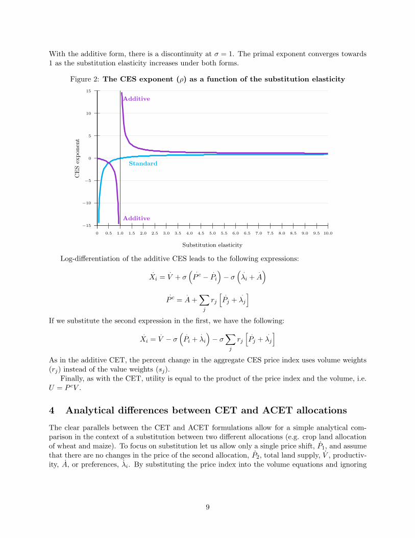
With the additive form, there is a discontinuity at σ = 1. The primal exponent converges towards1 as the substitution elasticity increases under both forms.

Figure 2: The CES exponent (ρ) as a function of the substitution elasticity

−15

−10

−5

0

5

10

15

0 0.5 1.0 1.5 2.0 2.5 3.0 3.5 4.0 4.5 5.0 5.5 6.0 6.5 7.0 7.5 8.0 8.5 9.0 9.5 10.0

Substitution elasticity

CESex

ponen

t

Standard

Additive

Additive

Log-differentiation of the additive CES leads to the following expressions:

.Xi =

.V + σ

( .

P c −.Pi

)

− σ( .λi +

.A)

.

P c =.A+

∑

j

rj

[ .Pj +

.λj

]

If we substitute the second expression in the first, we have the following:

.Xi =

.V − σ

( .Pi +

.λi

)

− σ∑

j

rj

[ .Pj +

.λj

]

As in the additive CET, the percent change in the aggregate CES price index uses volume weights(rj) instead of the value weights (sj).

Finally, as with the CET, utility is equal to the product of the price index and the volume, i.e.U = P cV .

4 Analytical differences between CET and ACET allocations

The clear parallels between the CET and ACET formulations allow for a simple analytical com-parison in the context of a substitution between two different allocations (e.g. crop land allocationof wheat and maize). To focus on substitution let us allow only a single price shift, P1, and assumethat there are no changes in the price of the second allocation, P2, total land supply, V , productiv-ity, A, or preferences, λi. By substituting the price index into the volume equations and ignoring

9

the variables that are assumed fixed, we can then rewrite the log-linearized versions of the CETand ACET as:

Xi = ω(Pi − s1P1) (16)

XAi = ωA(Pi − r1P1) (17)

where Xi and XAi are the CET and ACET allocations, respectively. We can then write an equation

for the relative difference between the volume results for allocations 1 and 2 as:

XA1

X1

=ωA

ω·(1− r1)

(1− s1)(18)

XA2

X2

=ωA

ω·r1s1

(19)

Notice that the relative percentage change in allocation between formulations, is independent of theprice shock and proportional to the difference in substitution parameters. Assuming substitutionparameters are identical this difference measure is also independent of the substitution parameter.However, it is important to note that absolute discrepancy (i.e. XA

i /Xi) will increase with thesubstitution parameter, ω. The relative percentage change in allocation only depends on thedifference between the volume and value shares, r1 and s1, respectively. In other words, it isonly dependent on whether P1 is greater or less than P2, where P1 and P2 are initial unit prices for1 and 2, respectively. We can make the following conclusions about sensitivity of the discrepancyto the initial prices:

• If the original shocked P1 < unshocked price P2 then r1 > s1 and the sensitivity of the ACETrelative to the CET is greater for the unshocked allocation 2 and less for shocked allocation1.

• If the original shocked P1 > unshocked price P2 then r1 < s1 and the sensitivity of the ACETrelative to the CET is less for the unshocked allocation 2 and greater for shocked allocation1.

In a similar fashion, we can explore the discrepancy between the total allocation in non-volumepreserving CET and the volume-preserving ACET using the following equation constructed fromthe initial equations, assuming identical substitution parameters (i.e. ωA = ω).

V

V A=

r1ω(P1 − s1P1) + r2ω(−s1P1)

r1ω(P1 − r1P1) + r2ω(−r1P1)=

r1 − s1(r1 − r2)

r1 − r1(r1 − r2)(20)

where only P1 is shocked. We can make the following conclusions:

• For P1 > P2 (i.e. s1 > r1) and r1 > r2, thenVV A

< 1 and the CET loses land

• For P1 > P2 (i.e. s1 > r1) and r1 < r2, thenVV A

> 1 and the CET gains land

• For P1 < P2 (i.e. s1 < r1) and r1 > r2, thenVV A

> 1 and the CET gains land

• For P1 < P2 (i.e. s1 < r1) and r1 < r2, thenVV A

< 1 and the CET loses land

10

Table 1: Initial values

Price Volume ValueWheat 1 25 25Maize 1 75 75Total 1 100 100

Finally, we can conclude that the direction of the individual CET and ACET allocation results(Xi and XA

i ) will be identical (i.e. the relative difference in allocation must be positive).Let us turn to a case where price shocks are present for both allocation prices; that is, P1 and

P2 are different from zero. Again, total allocation, productivity, and preferences remain fixed. Inthis case, the same relative difference measure can be written for allocation 1 as:

V A

V=

P1 − r1P1 − r2P2

P1 − s1P1 − s1P2

=P1 − r1P1 − P2 + r1P2

P1 − s1P1 − P2 + s1P2

=(P1 − P2)− r1(P1 − P2)

(P1 − P2)− s1(P1 − P2)(21)

The relationship above shows that in the case of dual shocks the direction of both CET andACET are identical, independent of the shock. Further, direction is preserved as long as thesubstitution parameters (ω and ωA) have the same sign. While these properties are convenient inthe case where total land allocation, productivity, and preferences are not changed, these convenientproperties do not necessarily hold when these variables are changed. Still, these properties help usexplain some of the results in the simple illustrative example and the application in Envisage thatfollow.

5 A numerical example of the additive CET

This section illustrates the additive CET with a small numerical example. Table 1 depicts aland supply choice between two sectors, called wheat and maize. The ’known’ data is the totalremuneration to land, i.e. the column under ’Value’. This is the data that would be incorporatedin a Social Accounting Matrix (SAM). In the absence of additional information—either prices orvolumes—the split of the value between price and volume is somewhat arbitrary and the standardapproach is to set prices to 1 and thus volumes and values coincide. In the example, wheat and maizehave respectively shares of 25 percent 75 percent share. In the sensitivity analysis below, we showthat making different assumptions about the price/volume split has no impact on a counterfactualexercise because in the case of the standard CET, only value shares matter. However, in the caseof the ACET, counterfactual shocks are sensitive to price initialization.

Table 2 reflects a limited set of sensitivity experiments using different assumptions on relativeprices and the elasticity of transformation. The top panel assumes that initial prices are identical(and equal to 1). The middle panel assumes that the initial price of land in maize is twice the price ofland in wheat. And the bottom panel assumes the reverse, i.e. that the price of wheat land is twicethe price of land. The table reflects a single experiment which is a doubling of the price of wheatland—under three different assumptions of the land transformation elasticity: 0.5, 1.0 and 2.0.Under each of the elasticity assumptions, the columns represent percent changes relative to specificvariables under the standard CET (labeled ’CET’) and the additive CET (labeled ’ACET’). Thetable reports the percent change in land supply to the wheat and maize markets, the discrepancybetween the sum of land supply to the individual markets and aggregate land supply, and thepercent change in the aggregate price of land and the land (dual) price index.

11

Table 2: Sensitivity analysis from a doubling of the price of wheat land, (percent)

ω = 0.5 ω = 1.0 ω = 2.0CET ACET CET ACET CET ACET

Unit prices initiallyWheat supply 24.7 28.2 51.2 60.0 103.8 128.6Maize supply -11.8 -9.4 -24.4 -20.0 -49.1 -42.9Land Discrepancy 2.7 0.0 5.5 0.0 10.8 0.0Price 28.5 32.0 32.3 40.0 40.1 57.1Price index 28.5 21.8 32.3 25.0 40.1 32.3

Initial price of maize = 2 × price of wheatWheat supply 24.7 21.3 51.2 42.9 103.8 81.8Maize supply -11.8 -14.2 -24.4 -28.6 -49.1 -54.5Land Discrepancy -2.8 0.0 -5.8 0.0 -12.1 0.0Price 28.5 25.0 32.3 25.0 40.1 25.0Price index 28.5 35.9 32.3 40.0 40.1 48.3

Initial price of wheat = 2 × price of maizeWheat supply 24.7 33.5 51.2 75.0 103.8 180.0Maize supply -11.8 -5.6 -24.4 -12.5 -49.1 -30.0Land Discrepancy 6.6 0.0 13.6 0.0 27.2 0.0Price 28.5 37.6 32.3 53.1 40.1 92.5Price index 28.5 12.2 32.3 14.3 40.1 19.5

Notice that the price initialization assumption has no impact on the results down the standardCET column, i.e. the results only depend on the value shares and are independent of the volumeshares. This is not the case with the additive CET formulation where the results are sensitive tothe price/volume splits.8

With the transformation elasticity set to 0.5, land supply for wheat increases by 25 percent andland supply for maize decreases by 12 percent. The land discrepancy row measures the deviationof the sum of land supply to each sector relative to aggregate land (which is invariant), i.e. theland discrepancy measure is 100(1 −

∑

iXi/V ). If it is positive, there is a ’loss’ of land, i.e. thesum of the components is less than total land. The discrepancy of land supply does vary with theprice initialization assumption. With the transformation elasticity at 0.5, the discrepancy is almost3 percent with the default initialization and 6.6 percent when the initial price of wheat land istwice the price of maize land. In the opposite case, when maize land is initially twice the price ofwheat land the discrepancy is nearly -2.8 percent, in other words, land supply to the two sectorsis greater than total land supply. The supply responsiveness using the additive CET is roughlycomparable with the standard CET with the low transformation elasticity, though the differencescan be important depending on price initialization (and the nature of the shock)—see for examplethe bottom panel.

The illustrative sensitivity analysis highlights a number of other points:

• The discrepancy rises with the transformation elasticity. In the final panel, with an elastic-ity of 2.0, the discrepancy is nearly 30 percent. Note that in practice land transformationelasticities tend to be relatively low, see for example Figure 6.2 in Hertel et al. (2009) where

8 The results of the additive CET would be insensitive if we hold the volume shares constant and adjust the valueshares.

12

the tiered transformation elasticities vary from 0.25 to 1. The default land transformationelasticity in the standard GTAP model is 1.9

• With low values for the transformation elasticities, both forms of the CET specificationprovide broadly similar orders of magnitudes in terms of the percent deviation from baselinevalues. The deviations become much greater as the transformation elasticity increases. In thethird panel, land for wheat increase by 180 percent in the case of a transformation elasticityof 2 with the additive version of the CET, whereas the increase is only 104 percent with thestandard CET. This is also where the discrepancy on land volumes is the highest.

• In the standard CET, there is no difference between the aggregate price and the aggregate(dual) price index. That is not the case with the additive CET where there can be sharpdeviations between the two.

In summary, with ”standard” transformation elasticities, the two formulations of the CETexhibit a behavior that is roughly comparable–though within limits if the price/volume splits areassumed to be important and plausible. In the bottom panel, with a transformation elasticity of1, the differences in the supply response are relatively significant as is the discrepancy in totalland use. The next section assesses the relative importance of the two formulations using theEnvisage model—comparing the land use implications in a baseline underlying current analysisof the economics of climate change.

6 Implications of the additive CET on land-use in Envisage

The sharp rise in agriculture and food prices in 2007/08 reinvigorated a policy focus on futurefood security after a relatively long period of dormant prices. The renewal of anxiety about foodsecurity also ties in with the increasing evidence of the impacts of climate change that will lead tohigher temperatures, changes in precipitation patterns and more frequent extreme weather events.A new network of scientists and economists focused on agriculture has been formed—known as theAgriculture Model Intercomparison and Improvement Project (AgMIP10)—that includes climatescientists, crop modelers and economic modelers. Their collective effort is intended to lead toimproved analysis within their respective disciplines and to promote more cross fertilization acrossdisciplines. One notable feature of the economic models of global agriculture is the wide dispersionin long-term projections for agricultural prices and land-use.11

Within the AgMIP context, the global economic modeling teams harmonized some of the ex-ogenous elements of the model in order to narrow the list of reasons for model differences. Har-monization centered on three key drivers—population and GDP growth and exogenous changes incrop yields. The first two were harmonized to the relatively new shared socio-economic pathways(SSPs)12 that have been developed for use by the Integrated Assessment Modeling (IAM) commu-nity. For the Phase 1 activities, the exogenous yield changes were provided by the InternationalFood Policy Research Institute (IFPRI) based on the Decision Support System for Agrotechnology

9 Dixon and Rimmer (2006) use a transformation elasticity in the case of labor markets of 2. In the case of CESelasticities, there are many examples of relatively high elasticities, for example Armington trade elasticities.

10 See www.agmip.org11 Phase 1 of the collective efforts of the global economic modeling teams is summarized in von Lampe et al. (2014).12 There are a number of references to the SSPs and the SSP process. See for example Moss et al.

(2010), Kriegler et al. (2012), O’Neill et al. (2012), van Vuuren et al. (2012) and O’Neill et al. (2014).The quantification of the GDP and population projections for the SSPs can be downloaded fromhttps://secure.iiasa.ac.at/web-apps/ene/SspDb.

13

Transfer (DSSAT) crop model13 coupled with climate models and an economic model linking yieldgrowth to R & D expenditures and GDP growth.

Phase 1 of the modeling intercomparison work of the global economic models was detailed ina special issue of Agricultural Economics that included an overview of the comparison exercise(von Lampe et al. (2014)) and chapters focused on specific modules of the global models, for ex-ample demand (Valin et al. (2014)), supply (Robinson et al. (2014)) and land-use (Schmitz et al.(2014)). The comparison project did lead to many improvements of the individual models andalso to a narrowing of the initial dispersion in the long-term projections—though the remainingdispersion was nonetheless significant.

The remainder of this section will focus on one of the model’s used in the AgMIP exercise—known as Envisage. The model was initially developed while the author was at the World Bankand was subsequently used by the Food and Agriculture Organization of the United Nations (FAO).Though still in use at both agencies, model development is mostly done at the Center for GlobalTrade Analysis (GTAP) at Purdue University. Version 8 of the model will be used for the analysisherein and uses as a starting point work undertaken by a subset of the AgMIP models in a USDAfunded project that resulted in a paper in Environmental Research Letters, see Wiebe et al. (2015).Compared to the Phase 1 simulations, those done for the ERL paper relied on a somewhat updatedGTAP database, the latest version of the SSP GDP and population projections and new projectionsfor the exogenous yield trends.

6.1 Land-use in Envisage

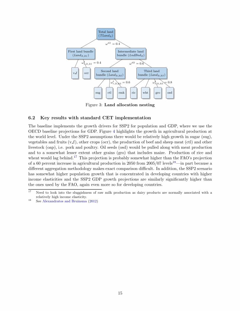
The land-use module in Envisage uses the land data available in the standard GTAP database—in this version land is only used in agriculture.14 Land is part of a nested production structurewith land demand substitutable with other factors of production (labor and capital) and alsosubstitutable with key inputs such as chemicals in crop production and feed in meat and dairyproduction.15 On the supply side, aggregate land for agriculture uses a logistic supply curve that iscalibrated to an initial elasticity of supply with an asymptote that provides a limit to the amountof usable land for agriculture. Aggregate agricultural land is then allocated to different uses using anested CET structure as depicted in figure 3.16 The top nest differentiates land-use for vegetablesand fruits and other crops from other uses—with a relatively low transformation elasticity of 0.4.The second nest differentiates sugar, cattle and raw milk from land used for cereals with an elasticityof 0.6. The final bundle includes cereals and oil seeds with a somewhat higher elasticity of 0.8.Land demand by sector is equated to land supply by sector and determines a sector-specific returnto land. In the standard model, there is no guarantee that the sum of land-use across sectors willequal aggregate land use.

13 See http://dssat.net/.14 Note that land use in the pork and poultry sectors is zeroed out and the land rents are imputed to capital

payments. We are also not using the AEZ satellite accounts that has land by activity broken out by AEZ, ofwhich there are up to 18 available per GTAP region.

15 See van der Mensbrugghe (2016) for a full specification of the Envisage model.16 This structure has been adapted from LEI’s MAGNET model.

14

Total land(TLand lt )

First land bundle(Land lt,lt1 )

v f ocr

Intermediate landbundle (LndBnd lt )

Second landbundle (Land lt,lt2 )

sug ctl rmk

Third landbundle (Land lt,lt3 )

ric wht gro osd

ωtl1 = 0.4

ωtr,lt,lt1

= 0.4 ωtl2 = 0.6

ωtr,lt,lt2

= 0.6 ωtr,lt,lt3

= 0.8

Figure 3: Land allocation nesting

6.2 Key results with standard CET implementation

The baseline implements the growth drivers for SSP2 for population and GDP, where we use theOECD baseline projections for GDP. Figure 4 highlights the growth in agricultural production atthe world level. Under the SSP2 assumptions there would be relatively high growth in sugar (sug),vegetables and fruits (v f), other crops (ocr), the production of beef and sheep meat (ctl) and otherlivestock (oap), i.e. pork and poultry. Oil seeds (osd) would be pulled along with meat productionand to a somewhat lesser extent other grains (gro) that includes maize. Production of rice andwheat would lag behind.17 This projection is probably somewhat higher than the FAO’s projectionof a 60 percent increase in agricultural production in 2050 from 2005/07 levels18—in part because adifferent aggregation methodology makes exact comparison difficult. In addition, the SSP2 scenariohas somewhat higher population growth that is concentrated in developing countries with higherincome elasticities and the SSP2 GDP growth projections are similarly significantly higher thanthe ones used by the FAO, again even more so for developing countries.

17 Need to look into the sluggishness of raw milk production as dairy products are normally associated with arelatively high income elasticity.

18 See Alexandratos and Bruinsma (2012)

15

Figure 4: Global output changes in baseline

ric wht gro osd sug v-f ocr ctl oap rmk

125

150

175

200

225

Productionindex

[2010=100]

2030 2050

Figure 5 highlights the Envisage Model’s projection for prices. These are measured as theaverage producer price weighted by regional production shares. The model’s numeraire is theaverage price of manufactured exports from high-income countries and thus the price increase isrelative to that index. With the exception of other crops and beef and sheep production, the priceincrease is relatively modest—though nonetheless positive. This would signify a reversal in thedecades long trend of moderately declining agricultural prices—notwithstanding the 2007/08 pricespike.19

Figure 5: Global price changes in baseline

ric wht gro osd sug v-f ocr ctl oap rmk

100

110

120

130

140

150

Price

index

[2010=100]

2030 2050

19 Data on commodity prices is available from the World Bank’s so-called Pink Sheet that can be downloaded fromhttp://www.worldbank.org/en/research/commodity-markets.

16

Figure 6 depicts the deviations in land supply generated by the CET in the year 2050, i.e.it measures 100(1 − V/

∑

i Xi) where V is the aggregate amount of land and Xi is land suppliedto activity i. The deviation at the global level is 3.5 percent a relatively small amount thatcould be ’adjusted’ away without causing too much concern, particularly given the overall noise inprojecting over a 40-year horizon. The deviations at the country level can be substantially greater,as highlighted in Fujimori et al. (2014). In the case of India (IND) the deviation is over 8 percentand it is around 5 percent for China (CHN), Indonesia (IDN) and Sub Saharan Africa (SSA). Asalluded to in the previous section, it is possible that the deviations could be significantly higher:1) if the land transformation elasticities are greater; 2) a different set of shocks is simulated; and3) under a different initialization of the land variables, i.e. the price/volume split initialization.Sensitivity analysis would be the recommended path for assessing the quantitative significanceof point 1. Different baseline assumptions could help elucidate the role of point 2, for examplehow sensitive are the deviations to changes in exogenous yield growth, differences in substitutionelasticities in the production function and/or the role of income and price elasticities. The role ofvariable initialization could also be readily assessed with the availability of a satellite data basewith land-use in volumes.

Figure 6: Land deviations

hic chn idn xea ind xsa rus tur xec mna ssa bra lax wld

0

1

2

3

4

5

6

7

8

9

Price

index

[2010=100]

6.3 Introduction of the additive CET

This section describes the key results from replacing the standard CET for land allocation withthe additive form of the CET. From the point of view of implementation—the switch is relativelypainless for the standard version of Envisage. In practical terms, we assume the same initializationof prices and volumes (with all initial prices set at 1). We use the same nesting for the allocationof land supply—see figure 3 and the same CET transformation elasticities. Hence the initializationand calibration code are identical with an additional initialization of the CET (dual) price indexvariable that is now differentiated from the aggregate price variable. The dual price index isinitialized to the initial aggregate price.20 The model specification requires two changes. The dualprice equation uses ω as the exponent rather than ω + 1. And the model needs an additionalequation to calculate the aggregate price derived from the zero profit condition.

20 The initialization of the dual price index is arbitrary as it in essence defines the initial utility level that isirrelevant to model results.

17

Figure 7 shows the impact on output in 2050 from implementing the additive CET comparedwith the standard CET. The impacts are shown across the model’s agricultural sectors and forbroad regional aggregates—global and developing and developed regions. The differences at theglobal level are relative small—most well within 1 percent. There are greater variations acrossregions—when comparing between developed and developing and that appear to offset each other.In the case of wheat, production is almost 2.5 percent higher in developing countries with theadditive CET, counterbalanced by a reduction of over 1.5 percent for developed countries and anaverage increase of about 1 percent at the global level.

Figure 7: Impact of the additive CET on output

ric wht gro osd sug v-f ocr ctl oap rmk

−3.0−2.5−2.0−1.5−1.0−0.50.00.51.01.52.02.53.0

Percentch

angein

2050relativeto

standard

CET

World Developing Developed

The impact on prices of using the additive CET is generally to lower agricultural prices—globallyand across the two broad income regions, figure 8. The impacts on prices are significantly higherfor developing countries—often around 4–5 percent and generally below 1 percent for developedcountries.

18

Figure 8: Impact of the additive CET on prices

ric wht gro osd sug v-f ocr ctl oap rmk

−5.0

−4.0

−3.0

−2.0

−1.0

0.0

Percentch

angein

2050relativeto

standard

CET

World Developing Developed

The impact on land-use can be relatively significant, figure 9. At the global level, the additiveCET increases aggregate land-use in 2050 by nearly 3 percent. At the regional level there are sharpvariations from negative or no change in the high-income (hic), rest of East Asia (xea), Russia(rus), Brazil (bra) and the rest of Latin America (lax). India (ind) has the highest percent changeat 9 percent, followed by China (chn), Indonesia (idn) and Sub Saharan Africa (SSA) at around5 percent. There is little difference in the impacts between land-use for crops and total agriculture.

19

Figure 9: Impact of the additive CET on land-use

hic chn idn xea ind xsa rus tur xec mna ssa bra lax wld

−10123456789

10

Percentch

angein

2050relativeto

standard

CET

Cropland All agriculture

7 Conclusion

With the increasing use of physical quantities in CGE models, the ubiquitous use of the CETand CES functions in model specification can lead to counter-intuitive results—particularly whensharing results across disciplines. Examples abound including labor and land markets, energy andpower, and potentially others such as fertilizers and water. The most widely used alternative to tothe CET/CES functions is the logit function that has been applied often in energy models and hasbeen more recently used in land-use models and one of its characteristics is volume additivity.

This paper explores a modified version of the CES/CET function that is volume preserving andrequires very modest changes in model implementation (and potentially none in model calibrationand elasticity estimates). Beyond the difference in the objective function that is being optimized,the key difference between the standard form and volume preserving forms is the interpretation ofthe dual price index. In the case of the standard form, the dual price index is equated to the priceof the aggregate volume and percent changes in the price index relates back to the initial valueshares of the components. In the case of the additive form, there is no equality between the dualprice index and the aggregate price, and percentage changes to the dual price index relate to theinitial volume shares. Thus in the standard form the results of a shock are invariant to the initialvolume/price split. This is not the case for the additive variant. Some of these issues were exploredusing a simple numerical example that also highlighted the role of the level of the elasticity indetermining the deviation from additivity.

The final section contrasted the use of the standard versus additive CET in the land-use moduleof the Envisage model that has been used to look at future scenarios for agriculture and food.Deviations from additivity in the standard model are relatively small at the global level, but can besignificant at the country or regional level. With the minor model modifications cited above, themodel results using the additive version of the CET induce some changes, but relatively modest,particularly when considering the 40-year time horizon. They are more variegated across sectors

20

and regions, suggesting the need for additional in-depth analysis as well as more sensitivity analysis.Three clear paths forward suggest themselves. The first is to run the same baseline simulation usingthe standard and additive forms of the CET but with different and presumably higher elasticities.21

A second strand would be to introduce a proper price/volume split for land-use. The small numericalexercise suggests that large price differences that would generate large initial deviations betweenvolume and value shares, could have a significant influence on the differences in impacts from usingone form over the other. A third direction would be to assess a wide variety of shocks—particularlythose that might lead to sharp changes in land-use. These might include some of the drivers in thebaseline scenario such as exogenous yield growth.

Despite the limited analysis of the use of the additive CET/CES described in this paper, itappears as a promising alternative to either the standard CET/CES or the logit. In the case ofthe former, it requires only a slight modification to the existing standard specification and withpotentially no change to the input elasticities. A more systematic analysis would be needed to seehow it compares with the logit—including ideally some back-casting exercise.

References

Alexandratos, N., and J. Bruinsma. 2012. “World Agriculture Towards 2030/2050: The 2012 Revi-sion.” ESA Working Paper No. 12-03, Food and Agriculture Organization of the United Nations(FAO), Rome. http://www.fao.org/docrep/016/ap106e/ap106e.pdf.

Bowles, S. 1970. “Aggregation of Labor Inputs in the Economics of Growth and Planning:Experiments with a Two-Level CES Function.” Journal of Political Economy 78:68–81.http://www.jstor.org/stable/1829620.

Dixon, P.B., and M.T. Rimmer. 2006. “The Displacement Effect of Labour-Market Programs:MONASH Analysis.” Economic Record 82:S26–S40. doi:10.1111/j.1475-4932.2006.00330.x.

—. 2003. “A New Specification of Labour Supply in the MONASH Model with an IllustrativeApplication.” Australian Economic Review 36:22–40. doi:10.1111/1467-8462.00265.

Edmonds, J., and J.M. Reilly. 1985. Global Energy: Assessing the Future. New York, NY: OxfordUniversity Press.

Fujimori, S., T. Hasegawa, T. Masui, and K. Takahashi. 2014. “Land use representation in aglobal CGE model for long-term simulation: CET vs. logit functions.” Food Security 6:685–699.doi:10.1007/s12571-014-0375-z.

Giesecke, J.A., N.H. Tran, E.L. Corong, and S. Jaffee. 2013. “Rice Land Designation Policy inVietnam and the Implications of Policy Reform for Food Security and Economic Welfare.” Journalof Development Studies 49:1202–1218. doi:10.1080/00220388.2013.777705.

Hertel, T.W., H. Lin, S. Rose, and B. Sohngen. 2009. “Modelling land use related greenhouse gassources and sinks and their mitigation potential.” In T. W. Hertel, S. K. Rose, and R. S. J. Tol,eds. Economic Analysis of Land Use in Global Climate Change Policy . Oxon, UK: Routledge,chap. 6, pp. 123–153.

21 It would also be worth pursuing analysis of other markets—for example the energy and power markets whereelasticities are likely to be higher, particularly if trade in these products is considered.

21

Kriegler, E., B.C. O’Neill, S. Hallegatte, T. Kram, R.J. Lempert, R.H. Moss, and T. Wilbanks.2012. “The need for and use of socio-economic scenarios for climate change analysis: A newapproach based on shared socio-economic pathways.” Global Environmental Change 22:807–822.doi:10.1016/j.gloenvcha.2012.05.005.

Kyle, P., P. Luckow, K. Calvin, W. Emanuel, M. Nathan, and Y. Zhou. 2011.“GCAM 3.0 Agriculture and Land Use Modeling: Data Sources and Methods.”Working paper No. 21025, Pacific Northwest National Laboratory (PNNL), December.http://wiki.umd.edu/gcam/images/2/25/GCAM_AgLU_Data_Documentation.pdf.

Moss, R.H., J.A. Edmonds, K.A. Hibbard, M.R. Manning, S.K. Rose, D.P. van Vuuren, T.R.Carter, S. Emori, M. Kainuma, T. Kram, G.A. Meehl, J.F.B. Mitchell, N. Nakicenovic, K. Riahi,S.J. Smith, R.J. Stouffer, A.M. Thomson, J.P. Weyant, and T.J. Wilbanks. 2010. “The NextGeneration of scenarios for climate change research and assessment.” Nature 463:747–756.

O’Neill, B.C., T.R. Carter, K.L. Ebi, J. Edmonds, S. Hallegatte, E. Kemp-Benedict, E. Kriegler,L. Mearns, R. Moss, K. Riahi, B. van Ruijven, and D. van Vuuren. 2012. “MeetingReport of the Workshop on The Nature and Use of New Socioeconomic Pathways forClimate Change Research.” Working paper, National Center for Atmospheric Research.https://www.isp.ucar.edu/sites/default/files/Boulder%20Workshop%20Report_0.pdf.

O’Neill, B.C., E. Kriegler, K. Riahi, K.L. Ebi, S. Hallegatte, T.R. Carter, R. Mathur, and D.P. vanVuuren. 2014. “A new scenario framework for climate change research: the concept of sharedsocioeconomic pathways.” Climatic Change 122:387–400. doi:10.1007/s10584-013-0905-2.

Perroni, C., and T.F. Rutherford. 1998. “A Comparison of the Performance of Flexible FunctionalForms for Use in Applied General Equilibrium Modelling.” Computational Economics 11:245–263. doi:10.1023/A:1008641723127.

—. 1995. “Regular flexibility of nested CES functions.” European Economic Review 39:335–343.doi:10.1016/0014-2921(94)00018-U, Symposium of Industrial Oganizational and Finance.

Peters, J.C. 2016. “GTAP-E-Power: An electricity-detailed extension of the GTAP-E model.”Presented at the 19th annual conference on global economic analysis, washington dc, usa, GlobalTrade Analysis Project (GTAP), Department of Agricultural Economics, Purdue University,West Lafayette, IN. https://www.gtap.agecon.purdue.edu/resources/download/7841.pdf.

Robinson, S., H. van Meijl, D. Willenbockel, H. Valin, S. Fujimori, T. Masui, R. Sands, M. Wise,K. Calvin, P. Havlık, D. Mason d’Croz, A. Tabeau, A. Kavallari, C. Schmitz, J. Dietrich, andM. von Lampe. 2014. “Comparing supply-side specifications in models of global agriculture andthe food system.” Agricultural Economics 45:21–35. doi:10.1111/agec.12087.

Schmitz, C., H. van Meijl, P. Kyle, G.C. Nelson, S. Fujimori, A. Gurgel, P. Havlık, E. Heyhoe,D. d’Croz Mason, A. Popp, R. Sands, A. Tabeau, D. van der Mensbrugghe, M. von Lampe,M. Wise, E. Blanc, T. Hasegawa, A. Kavallari, and H. Valin. 2014. “Land-use change trajectoriesup to 2050: insights from a global agro-economic model comparison.” Agricultural Economics

45:69–84. doi:10.1111/agec.12090.

Valin, H., R.D. Sands, D. van der Mensbrugghe, G.C. Nelson, H. Ahammad, E. Blanc, B. Bodirsky,S. Fujimori, T. Hasegawa, P. Havlık, E. Heyhoe, P. Kyle, D. Mason D’Croz, S. Paltsev, S. Rolin-ski, A. Tabeau, H. van Meijl, M. von Lampe, and D. Willenbockel. 2014. “The future of food

22

demand: understanding differences in global economic models.” Agricultural Economics 45:51–67. doi:10.1111/agec.12089.

van der Mensbrugghe, D. 2016. “The Environmental Impact and Sustainability Applied GeneralEquilibrium (ENVISAGE) Model. Version 9.0.” Unpublished manuscript, Center for GlobalTrade Analysis (GTAP), Department of Agricultural Economics, Purdue University, WestLafayette, IN.

van Vuuren, D.P., M.T. Kok, B. Girod, P.L. Lucas, and B. de Vries. 2012. “Scenarios in Global En-vironmental Assessments: Key characteristics and lessons for future use.” Global Environmental

Change 22:884–895. doi:10.1016/j.gloenvcha.2012.06.001.

von Lampe, M., D. Willenbockel, H. Ahammad, E. Blanc, Y. Cai, K. Calvin, S. Fujimori,T. Hasegawa, P. Havlık, E. Heyhoe, P. Kyle, H. Lotze-Campen, D. Mason d’Croz, G.C. Nelson,R.D. Sands, C. Schmitz, A. Tabeau, H. Valin, D. van der Mensbrugghe, and H. van Meijl. 2014.“Why do global long-term scenarios for agriculture differ? An overview of the AgMIP GlobalEconomic Model Intercomparison.” Agricultural Economics 45:3–20. doi:10.1111/agec.12086.

Wiebe, K., H. Lotze-Campen, R. Sands, A. Tabeau, D. van der Mensbrugghe, A. Biewald,B. Bodirsky, S. Islam, A. Kavallari, D. Mason-D’Croz, C. Muller, A. Popp, R. Robertson,S. Robinson, H. van Meijl, and D. Willenbockel. 2015. “Climate change impacts on agricul-ture in 2050 under a range of plausible socioeconomic and emissions scenarios.” Environmental

Research Letters 10:085010. http://stacks.iop.org/1748-9326/10/i=8/a=085010.

23