volume iii analysis of buckling
TRANSCRIPT

1/3/2012 C:\W\whit\Classes\306\Notes\3_Buckling\1_buckling.docx 1 of 2
Volume III Analysis of Buckling
1/4/2012 p. 1 of 113

1/3/2012 C:\W\whit\Classes\306\Notes\3_Buckling\1_buckling.docx 2 of 2
The notes on buckling have two options for deriving the buckling equations. One is based on
total potential energy and the other virtual work. If there is time, the total potential energy
approach has the advantage of giving more breadth to the course. The virtual derivation has
the advantage of being a direct extension of what has already been covered, so it takes less
time. The major sections of notes are as follows: (Choose Version1 or 2 and then proceed with
the rest of the notes.)
Version 1: Introduction to buckling based on virtual work
o Unique to this version: coverage of nonlinear coupling of extension and bending
Version 2: Introduction to buckling based on total potential energy
o Unique to this version: much more coverage of stability of mechanisms
o I will probably leave this version out of your notes to avoid confusion.
Regardless of how one obtains the governing equations, they are the same. Hence, the
following is independent of whether Total Potential Energy or Virtual Work was selected above.
Classical beam buckling
Finite element analysis of beam buckling
Buckling of a frame (theory and ABAQUS)
Buckling of plates (ABAQUS)
Page #
Virtual Work Formulation…………………………………………………………………………….
o Nonlinear Analysis of Beam Using Differential Equation…………………..
o Derivation of Nonlinear Virtual Work Equation…………………………………
Nonlinear and “Linear Buckling” Analysis……………………………..
Classical Virtual Work……………………………………………….
Single FEA Model………………………………………………………
o Buckling of Mechanisms…………………………………………………………………..
o Examples of Buckling Analysis of Mechanisms and Beams………………..
Total Potential Energy Formulation………………………………………………………………
1/4/2012 p. 2 of 113

12/29/2011 C:\W\whit\Classes\306\Notes\3_Buckling\1_BucklingIntro_VirtualWork\1_buckling_VirtualWork.docx 1 of 14
Introduction to Buckling Analysis
Derivation of Equations Based on Virtual Work Buckling (often referred to as loss of stability) refers to a large increase in displacement when there is a small increment in load. To illustrate the phenomena, we will start by performing a nonlinear analysis of a beam with a distributed transverse load and an axial load. We will observe a highly nonlinear behavior when the axial load is too large. We can identify a load level that is “critical”.
Then we will consider what happens when there is no transverse load, but still an axial load. Note that if linear analysis is performed for this axial loading, the response is very simple. This is not the case when we consider even the simplest approximation that accounts for nonlinearity. The analysis of such configurations is referred to as buckling analysis. (More accurately, it is referred to as linear buckling analysis, but we will not get into why.)
We will derive matrix formulas for performing buckling analysis that are like what we derived for linear analysis, except for an additional term.
Here are a few pictures that illustrate buckling of “beams”.
http://en.wikipedia.org/wiki/Sun_kink
Spoorspatting_Landgraaf.jpg
1/4/2012 p. 3 of 113

12/29/2011 C:\W\whit\Classes\306\Notes\3_Buckling\1_BucklingIntro_VirtualWork\1_buckling_VirtualWork.docx 2 of 14 Why are we interested in buckling ?
In most structures the displacements increase gradually with increased applied load. If the applied load is too large (particularly for compressive structures), a small increase in applied load can lead to a sudden large increase in the displacements. Buckling refers to this transition to large, often catastrophic displacements. Buckling can occur due to thermal or mechanical loads. Sometimes this abrupt behavior can be exploited for useful purposes.
Buckling is one type of instability. Instability is a state in which small perturbations (e.g. small increments in load) can cause large changes in the response of the structure. Instability can be due to geometric effects (as is usually the case in buckling) or change in material properties. (e.g. material yielding or failure) Instability occurs in a variety of physical systems other than structures, such as those involving heat transfer and fluid flow. In this course we will limit ourselves to instability of structures due buckling.
Examples of buckling • collapse of yardstick due to excess axial load • collapse of assemblage of white-board markers due to excess axial load • buckling of roads on hot days • collapse of large towers (comprised of trusses and stay wires) • bi-metallic strip used for thermostat • truss bridges • collapse of thin shell (Coke can) • etc.
1/4/2012 p. 4 of 113

12/29/2011 C:\W\whit\Classes\306\Notes\3_Buckling\1_BucklingIntro_VirtualWork\1_buckling_VirtualWork.docx 3 of 14
Nonlinear Analysis of a Beam
The load for the plots below = lambda * Pcritical => When lambda = 1.0, the buckling load has been reached. We have not discussed how to determine the buckling load yet, but we will very soon. Note that the load at which displacement heads for infinity does not depend on the magnitude of the transverse distributed load q. See the Maple worksheet beamNonlinear_ODE.mws to see the details of the solution. The governing differential equation (for this particular problem) is derived at the end of this file. The general differential equation and the virtual work are derived in 3_derivation_DEQN_VirtualWork.docx. Also, this problem has been solved using a single finite element and the results summarized in the file 4_beamNonlinear_FEA.docx. These last two files are the next files in your notes.
Distributed load intensity = 1 Distributed load intensity = 5
For both cases, the displacement
becomes very large when the load approaches Pcritical (i.e. lambda =1 .0)
1/4/2012 p. 5 of 113

12/29/2011 C:\W\whit\Classes\306\Notes\3_Buckling\1_BucklingIntro_VirtualWork\1_buckling_VirtualWork.docx 4 of 14 Derivation of equilibrium equation for this particular problem (… see general derivation next)
1/4/2012 p. 6 of 113

12/29/2011 C:\W\whit\Classes\306\Notes\3_Buckling\1_BucklingIntro_VirtualWork\1_buckling_VirtualWork.docx 5 of 14
Derivation of Nonlinear Beam Equations Using Differential Element
In 306 we will always be able to obtain P(x) from statics. In general, a stress analysis would have to be done first to determine P(x).
( )
1) 0 2) 0 3) 0
1) 0 0
2) 0 0
3) Sum moments about centroid
*offset between axial forces =
2 2
( ) ( )2 2
x y
x x
y y
F F MdPP P dP f dx fdxdVV V dV f dx fdx
dv dxdx
dx dxM M dM V V dV
dv dx dv dxP P dPdx dx
Σ = Σ = Σ =
− + + + = ⇒ + =
− + + + = ⇒ + =
− + + + + +
+ − − +
0=
1 02 2
Eliminate high order terms
0
Now we could calculate the weak directly from the DEQNS. (alternative=subject differential element to virtual displacements and add u
dM dV dv dvV P dPdx dx dx
dM dvV Pdx dx
+ + − − =
+ − =
p the virtual work. This is the "306" way.)
1/4/2012 p. 7 of 113

12/29/2011 C:\W\whit\Classes\306\Notes\3_Buckling\1_BucklingIntro_VirtualWork\1_buckling_VirtualWork.docx 6 of 14 Very Important! This derivation assumes that the axial force "P" is positive if it is tensile. If we assume P is positive when it is compressive, then simply change the sign of P in the equations above.
Hence, the governing differential equations are
0
0 Note that
ydV fdxdM dv dMV P Vdx dx dx
+ =
+ − = ≠
Derivation of Virtual Work from FBD
Impose virtual vertical translation and rotation of the differential element shown on the previous page. We have done this before for the linear case. The only new contribution is from P. The contribution to the VW due to P is as follows:
( ) ( )
( )
1 12 2
12
. . .
contribution to VW = - since
Pdv dvdVW dx P dP dx Pdx dx
dv dx P dP Pdx
dv dx P H O Tdx
dv dv dvP dxdx dx dx
δθ δθ
δθ
δθ
δ θ
= − + + −
= − + + = − −
=> ≈∫
When we derive the matrix form of the equations, we will see that this is a contribution to the stiffness matrix of
ji dNdNP dxdx dx∫
The matrix Kσ is often referred to as the geometric stiffness matrix, since it is related to geometric
nonlinearity.
Comment: The lateral deflection causes a shortening of the beam-column, but we still obtain ( )P P dP uδ− + + for the virtual work due to P. This is the same as for a linear uniaxial rod unless we
use the nonlinear strain displacement in writing P. In this class (aero 306) we will typically know the axial force distribution P… either by inspection or from simple statics.
1/4/2012 p. 8 of 113
12/29/2011 C:\W\whit\Classes\306\Notes\3_Buckling\1_BucklingIntro_VirtualWork\1_buckling_VirtualWork.docx 7 of 14
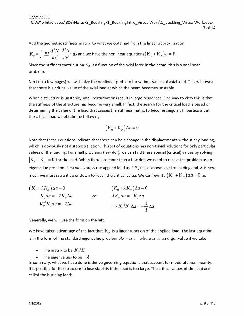
Add the geometric stiffness matrix to what we obtained from the linear approximation 22
0 2 2ji d Nd NK EI dx
dx dx= ∫ and we have the nonlinear equations ( )0K K F.aσ+ =
Since the stiffness contribution Kσ is a function of the axial force in the beam, this is a nonlinear problem.
Next (in a few pages) we will solve the nonlinear problem for various values of axial load. This will reveal that there is a critical value of the axial load at which the beam becomes unstable.
When a structure is unstable, small perturbations result in large responses. One way to view this is that the stiffness of the structure has become very small. In fact, the search for the critical load is based on determining the value of the load that causes the stiffness matrix to become singular. In particular, at the critical load we obtain the following
( )0K K 0aσ+ ∆ =
Note that these equations indicate that there can be a change in the displacements without any loading, which is obviously not a stable situation. This set of equations has non-trivial solutions for only particular values of the loading. For small problems (few dof), we can find these special (critical) values by solving
0K K 0σ+ = for the load. When there are more than a few dof, we need to recast the problem as an
eigenvalue problem. First we express the applied load as Pλ , P is a known level of loading and λ is how
much we must scale it up or down to reach the critical value. We can rewrite ( )0 K 0aσΚ + ∆ = as
( )0
01
0
0 K K aK a K aK K a a
σ
σ
σ
λλ
λ−
+ ∆ =
∆ = − ∆
∆ = − ∆
or
( )0
0
10
0
1
K K aK a K a
K K a a
σ
σ
σ
λλ
λ−
+ ∆ =
∆ = − ∆
=> ∆ = − ∆
Generally, we will use the form on the left.
We have taken advantage of the fact that Kσ is a linear function of the applied load. The last equation
is in the form of the standard eigenvalue problem where is an eigenvalueAx xα α= if we take
• The matrix to be 10K Kσ
− • The eigenvalues to be λ−
In summary, what we have done is derive governing equations that account for moderate nonlinearity. It is possible for the structure to lose stability if the load is too large. The critical values of the load are called the buckling loads.
1/4/2012 p. 9 of 113

12/29/2011 C:\W\whit\Classes\306\Notes\3_Buckling\1_BucklingIntro_VirtualWork\1_buckling_VirtualWork.docx 8 of 14 Note that I used the phrase “buckling loads”, not the singular form. When one solves a multi-dof problem, multiple critical values of the load will be calculated that correspond to particular buckling modes (deformed shapes). For simple structures, this is just an interesting mathematical oddity, since the structure is destroyed once the smallest buckling load is reached. For more complex configurations, the structure actually only loses part of its stiffness when the “critical load” is reached and it is possible to reach other “critical loads”.
1/4/2012 p. 10 of 113

12/29/2011 C:\W\whit\Classes\306\Notes\3_Buckling\1_BucklingIntro_VirtualWork\1_buckling_VirtualWork.docx 9 of 14
Appendix
Alternate Derivations
These are for those of you that are a bit more curious. Only read if you already understand the previous derivation.
Alternate derivation 1
Rather than repeat what we did previously for the linear case, note two things:
1) When we calculate the virtual work for the differential element for the linear case, we obtained the following:
0
0
ydV f vdxdxdM dvV dxdx dx
δ
δ
+ = + =
∫
∫
2) The only difference we have for this approximate nonlinear analysis is the additional term in the second equation. Let’s see how this contributes to the virtual work and eventually the matrix equations.
where we assumed
ii
i i
dNdv dv dvP dx a P dxdx dx dx dx
v N a
δ δ− = −Σ
= Σ
∫ ∫
Recall that we factored out the іaδΣ before and set the coefficient to zero. Hence, the contribution to
the equilibrium equation is
- idNdvP dxdx dx∫
Now put the approximation for v into this integral:
where K
j ji ij j
j
ji
dN dNdN dNP a dx P dx a K adx dx dx dx
dNdNP dxdx dx
σ
σ
Σ = − = −
=
∑∫ ∫
∫
Alternate derivation 2
1/4/2012 p. 11 of 113

12/29/2011 C:\W\whit\Classes\306\Notes\3_Buckling\1_BucklingIntro_VirtualWork\1_buckling_VirtualWork.docx 10 of 14 When the differential element deforms, there is axial displacement that is strictly due to the rigid body rotation. If we assume the beam is inextensible (i.e. along the neutral axis the axial strain is zero), then all of the axial displacement is due to the rotation. The virtual work is
. . .
( )left right
right left
P u P u H O TP u uδ δ
δ δ
− + +
= −
Hence, we need to obtain an expression for amount of stretch that occurs in the x-direction during deformation and then take the variation of it. Note that the stretch will be negative, since the projection on the x-axis must shrink during rotation. The amount of axial displacement can be calculated as follows:
22 2 2 2
1/22 2
1
11 1 (Taylor series approximation)2
Since the beam is asumed to be inextensible, = original projection on
dvds dx dv dxdx
dv dvds dx dxdx dx
ds
= + = +
=> = + ≈ +
2
the x-axis
1=> projection shrinks by 2
dvds dx dxdx
− =
Recall that the virtual work contribution is ( )right leftP u uδ δ− , which = P*(variation of lengthening of
projection on x-axis).
21variation of lengthening of projection on x axis2
dv dv dvdx dxdx dx dx
δ δ − = − = −
Hence the contribution to the virtual work for the differential element is
dv dvP dxdx dx
δ− . Integrate this to get the total contribution. The result is that the total internal virtual
work (including that from the linear contributions) is 2 2
2 2
dv dv d v d vP dx EI dxdx dx dx dx
δ δ− −∫ ∫
This is identical to what we obtained earlier. It might have seemed that in the first derivations we were ignoring the axial displacements… and in fact we were. What we did not ignore in the first derivation was the variation of the axial displacements which were due to the virtual rotation. This is all we needed to calculate the virtual work due to P. In the second derivation we calculated the axial displacements and then used them only for determining the variation of the axial displacement.
Alternate derivation 3 using Green-Lagrange strain (this is a bit advanced)
1/4/2012 p. 12 of 113

12/29/2011 C:\W\whit\Classes\306\Notes\3_Buckling\1_BucklingIntro_VirtualWork\1_buckling_VirtualWork.docx 11 of 14 The linear strain-displacement relations are valid only for infinitesimal displacements and rotations. There is another measure of strain that is still valid when there is finite rotation. The meaning of this strain measure is the same as for the linear strain measures as long as the strains are infinitesimal. These measures of strain are called the Green-Lagrange strains. For the normal strain n the x-direction, the formula for 2D is
2 21
2xxu u vx x x
ε ∂ ∂ ∂ = + + ∂ ∂ ∂
For the first order approximation of nonlinear beam behavior, one normally ignores the term2u
x∂
∂ and
so the formula simplifies to 21
2xxu vx x
ε ∂ ∂ = + ∂ ∂ . Recall that the internal virtual work for a uniaxial rod is
xx xxEA dxε δε−∫ . For the uniaxial rod we assumed that the axial displacement is constant over the
cross section. If we relax this assumption, we can obtain a formula for the internal virtual work for a
beam. In particular, let’s assume that 0( , ) ( ,0) dv dvu x y u x y u ydx dx
= − ≡ − . Since there is variation
in the y-direction, we need to integrate in both the x- and y-directions. That is, the internal virtual work
for a beam is /2
0 /2
L h
xx xxhEb dydxε δε
−−∫ ∫ .
Substitute the expression for the displacement u(x, y) into the formula for the strain and we will obtain 22
02
12xx
u v vyx x x
ε ∂ ∂ ∂ = − + ∂ ∂ ∂ .
Note that 2
02xx
u v v vyx x x x
δε δ δ δ∂ ∂ ∂ ∂= − +
∂ ∂ ∂ ∂
Using this nonlinear formula for the strain in the integrals for virtual work will give us the virtual work for a nonlinear beam that includes extension and flexure.
1/4/2012 p. 13 of 113

12/29/2011 C:\W\whit\Classes\306\Notes\3_Buckling\1_BucklingIntro_VirtualWork\1_buckling_VirtualWork.docx 12 of 14
( )2 2 /2int0 /2
/2
0 /2
/2
0 /2
If the applied loads are not a function of the deformation state, thenL h
ij xx xxhi j i j
L h xxxxh
j i
L h xx xxh
j i
VWK Eb dydxq q q q
Eb dydxq q
Eb dydxq q
ε δεδ δ
δεεδ
ε δεδ
−
−
−
∂ ∂= − = − −
∂ ∂ ∂ ∂
∂∂= ∂ ∂
∂ ∂= +
∂ ∂
∫ ∫
∫ ∫
∫ ∫2/2
0 /2
2/2
0 /2
L h xxxxh
i j
L h xx xx xxh
j i i j
Eb dydxq q
Eb dydx F dxq q q q
δεεδ
ε δε δεδ δ
−
−
∂∂ ∂
∂ ∂ ∂= +
∂ ∂ ∂ ∂
∫ ∫
∫ ∫ ∫
If the beam is symmetric, some terms cancel and we are left with just
( )22
02
1 axial strain along neutral axis2
dud v dvM EI F EA EAdx dx dx
= = + =
If the loads are a function of the deformation state, then
2
iji j
VWKq qδ
∂= −
∂ ∂
…to be continued
Maple notebook that illustrates use of Green-Lagrange strain
….end of Appendix
1/4/2012 p. 14 of 113
12/29/2011 C:\W\whit\Classes\306\Notes\3_Buckling\1_BucklingIntro_VirtualWork\1_buckling_VirtualWork.docx 13 of 14
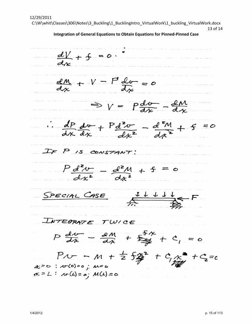
Integration of General Equations to Obtain Equations for Pinned-Pinned Case
1/4/2012 p. 15 of 113

12/29/2011 C:\W\whit\Classes\306\Notes\3_Buckling\1_BucklingIntro_VirtualWork\1_buckling_VirtualWork.docx 14 of 14
1/4/2012 p. 16 of 113

> >
(2.2)(2.2)
> >
> >
(2.1)(2.1)
(1.1)(1.1)
4a_beamNonlinear_classical.mwtransverse and axial load
The formulas used to account for nonlinearity assume only moderate nonlinearity=> large displacementscannot be predicted accurately.
Utility routinerestart:currentdir(); with(linalg):with(plots):
"C:\W\whit\Classes\306\Notes\3_Buckling\1_BucklingIntro_VirtualWork"
Get valid approximation (need to satisfy v(0)=0, v(L)=0)We will use a cubic approximation, which results in a 2-term solution.
v:= c1+ c2*x + c3*x^2+c4*x^3:v0 := subs(x=0,v):vL := subs(x=L,v):ans:=solve({v0=0,vL=0},{c1,c2,c3,c4}):v := subs(ans,v):print(`Valid assumed solution: v(x)=`,v);
Valid assumed solution: v(x)=, Kc4 L2Kc3 L xCc3 x2Cc4 x3
Now calculate derivatives and the variations of v and the derivativesvx := diff(v,x);vxx:= diff(vx,x);del_v := diff(v, c3) * del_c3 + diff(v, c4) * del_c4;del_vx := diff(vx, c3) * del_c3 + diff(vx, c4) * del_c4;del_vxx := diff(vxx,c3) * del_c3 + diff(vxx,c4) * del_c4;
vx := Kc4 L2Kc3 LC2 c3 xC3 c4 x2
vxx := 2 c3C6 c4 x
del_v := KL xCx2 del_c3C KL2 xCx3 del_c4
del_vx := KLC2 x del_c3C KL2C3 x2 del_c4
del_vxx := 2 del_c3C6 x del_c4
Calculate the virtual work, the governing equations, and solve them
1/4/2012 p. 17 of 113

(3.2)(3.2)
> >
> >
> >
(3.4)(3.4)
(3.3)(3.3)
(3.1)(3.1)
> >
We are assuming that the internal axial force "F" is constant in the structure.VW := int(f * del_v, x=0..L) - int(EI * vxx * del_vxx,x=0..L) -int(F*vx*del_vx,x=0..L);
VW := 14
f del_c4 L4C13
f del_c3 L3C12
f KL del_c3KL2 del_c4 L2
K12 EI c4 del_c4 L3K12
12 EI c3 del_c4C12 EI c4 del_c3 L2K4 EI c3 del_c3 L
K95
F c4 del_c4 L5K14
6 F c3 del_c4C6 F c4 del_c3 L4K13
3 F Kc4 L2
Kc3 L del_c4C4 F c3 del_c3C3 F c4 KL del_c3KL2 del_c4 L3K12
2 F
Kc4 L2Kc3 L del_c3C2 F c3 KL del_c3KL2 del_c4 L2KF Kc4 L2Kc3 L
KL del_c3KL2 del_c4 L
We have two equations:eq1 := diff(VW, del_c3)=0;eq2 := diff(VW, del_c4)=0;
eq1 := K16
f L3K6 EI c4 L2K4 EI c3 LK 32
F c4 L4K13
4 F c3K3 F c4 L L3
K12
2 F Kc4 L2Kc3 L K2 F c3 L L2CF Kc4 L2Kc3 L L2 = 0
eq2 := K14
f L4K12 EI c4 L3K6 EI c3 L2K95
F c4 L5K12
F c3 L4K13
3 F Kc4 L2
Kc3 L K3 F c4 L2 L3CF Kc4 L2Kc3 L L3 = 0
Solve the equations to obtain the unknowns c3 and c4ans := solve({eq1,eq2},{c3,c4});
ans := c3 =K12
f L2
12 EICF L2 , c4 = 0
Hence, our solution for the deflection is as follows. v := subs(ans, v);
v := 12
f L3 x12 EICF L2 K
12
f L2 x2
12 EICF L2
Note that the displacement is a linear function of the transverse load and a nonlinear function of the axial load.Since we have already plotted the exact solution previously in the notes, I will not repeat it here.Next we will predict the critical (buckling) loads.
Critical load
Note that this stiffness matrix is different than what we will obtain using FEA interpolation, but the
1/4/2012 p. 18 of 113

> >
(4.1)(4.1)
(4.3)(4.3)
> >
> >
(4.2)(4.2)
answer is the same, since both used cubic approximation.K := [ [diff(VW, del_c3,c3),diff(VW, del_c3,c4)], [diff(VW, del_c4,c3),diff(VW, del_c4,c4)] ]: print(`The stiffness matrix = `,evalm(K));print(`Note that the stiffness matrix does not depend on the transverse load, f`);
The stiffness matrix = ,K4 EI LK 1
3 F L3 K6 EI L2K
12
F L4
K6 EI L2K12
F L4 K12 EI L3K45
F L5
Note that the stiffness matrix does not depend on the transverse load, f
criticalLoads := solve(det(K)=0,F);
criticalLoads := K60 EI
L2 , K12 EI
L2
For comparison, the exact answer for the lowest buckling load = π
2 EI
L2
Pi^2*EI/L^2:print(`This evaluates to `, evalf(%));
This evaluates to , 9.869604404 EI
L2
This means that our cubic approximation is significantly overpredicting the buckling load. We need a higher order approximation to get a good solution.
1/4/2012 p. 19 of 113

12/29/2011C:\W\whit\Classes\306\Notes\3_Buckling\1_BucklingIntro_VirtualWork\4b_beamNonlinear_FEA.docx 1 of 3 Summary of Maple Worksheet
These results are from the file beamNonlinear_FEA.mws
The problem was also solved using Classical Virtual Work in the file beamNonlinear_classical.mws. Since a cubic approximation was used, the solution is the same as for the single finite element. In this document, numerical values of the parameters were used.
EI=32552. (Transverse load does not affect the critical load.)
Finite element formulas
Linear stiffness, K =
Ksigma =
Equivalent nodal loads=
12 EIL3
6 EIL2 −
12 EIL3
6 EIL2
6 EIL2
4 EIL −
6 EIL2
2 EIL
−12 EI
L3 −6 EIL2
12 EIL3 −
6 EIL2
6 EIL2
2 EIL −
6 EIL2
4 EIL
6 F5 L
F10 −
6 F5 L
F10
F10
2 F L15 −
F10 −
F L30
−6 F5 L −
F10
6 F5 L −
F10
F10 −
F L30 −
F10
2 F L15
, , ,f L
2L2 f12
f L2 −
L2 f12
1/4/2012 p. 20 of 113
12/29/2011C:\W\whit\Classes\306\Notes\3_Buckling\1_BucklingIntro_VirtualWork\4b_beamNonlinear_FEA.docx 2 of 3
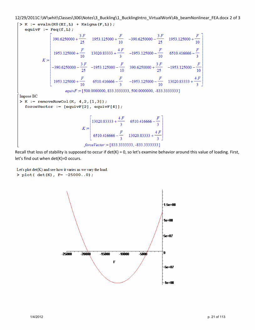
Recall that loss of stability is supposed to occur if det(K) = 0, so let's examine behavior around this value of loading. First, let’s find out when det(K)=0 occurs.
1/4/2012 p. 21 of 113

12/29/2011C:\W\whit\Classes\306\Notes\3_Buckling\1_BucklingIntro_VirtualWork\4b_beamNonlinear_FEA.docx 3 of 3 Note that det(K) =0 for two values of axial force F. There are two “critical” values that correspond to two modes (shapes) of buckling. Here is the nonlinear behavior
These displacements are getting large, but they are predicted to go to infinity as we approach the critical load, as shown below.
The worksheet also illustrates how one can exploit symmetry, but that material is optional and is not included in this file.
1/4/2012 p. 22 of 113

12/29/2011 C:\W\whit\Classes\306\Notes\3_Buckling\1_BucklingIntro_VirtualWork\5_mechanismBuckling.docx 1 of 2
Buckling of a Mechanism
Previously, we derived the conditions for buckling of a beam. We found that the critical load was determined by examining when the stiffness matrix became singular (e.g. 0ijK = ).
When we studied mechanisms early in the class, we did not generally bother to define a stiffness matrix. Part of the reason is because the problems were generally nonlinear… and the problems were generally single dof problems, so it was not worth the trouble. Now there is a reason to define a stiffness matrix.
When a structure exhibits “geometric nonlinearity”, the stiffness depends on the deformation state. In fact, there are two types of stiff nesses: secant stiffness and tangent stiffness. For a single dof problem, the secant stiffness is simply force/displacement. The tangent stiffness is the increment in force due to an increment in displacement. When predicting buckling, it is the tangent stiffness that is of interest. What we set out to determine is when there can be a change in displacements without there being a change in forces. Such a state is unstable.
Consider the following:
The virtual work consists of external virtual work due to the applied load and internal virtual work due to the deformation of the body. At equilibrium, there is a balance between the virtual work of the applied loads and that due to deformation (VW=0). Because the virtual work is linearly related to the variation of the dof, we can obtain the equilibrium equations by taking partial derivatives as follows: (The iq are the dof.)
0i
VWqδ
∂=
∂
If we can change the magnitudes of the dof without changing the loads, the system is
unstable. This corresponds to the case that 0j i
VWq qδ ∂ ∂
= ∂ ∂
The incremental stiffness of the system for a multiple dof problem is
2
iji j
VWKq qδ
∂= −
∂ ∂
Hence, the buckling load is obtained from the condition 0ijK = where ijK is the incremental or
tangential stiffness matrix for the system and is given by 2
iji j
VWKq qδ
∂= −
∂ ∂. I have used the terms
incremental and tangential stiffness. For linear problems, there is only one stiffness. For
1/4/2012 p. 23 of 113

12/29/2011 C:\W\whit\Classes\306\Notes\3_Buckling\1_BucklingIntro_VirtualWork\5_mechanismBuckling.docx 2 of 2
nonlinear problems, there is a secant stiffness, which for a single dof problem = forcedisplacement
.
There is also an incremental or tangential stiffness, which = forcedisplacement∆
∆. Strictly speaking,
for buckling analysis it is the incremental stiffness that determines stability, so the formula 2
iji j
VWKq qδ
∂= −
∂ ∂is applicable.
Alternate derivation
The equilibrium requirement is that Virtual Work=0. Since the Virtual Work is a linear function of the virtual displacements iqδ and the virtual displacements are arbitrary and independent, the
equilibrium equations are 0i
VWqδ
∂=
∂.
Now let’s rewrite this slightly: and 0i ii
VWq
ψ ψδ
∂= =
∂. The iψ are the residual forces and
must equal zero for there to be equilibrium. Now calculate the change in residual forces due to changes in the displacements. This would be a collection of stiffness terms.
iij
j
Kqψ∂
=−∂
If changing the displacements only (note the partial derivative) causes no change in the residual forces, something is wrong. In particular, the system is unstable. This corresponds to 0ijK = .
Note: The calculation of the stiffness matrix using 2
iji j
VWKq qδ
∂= −
∂ ∂ is also valid
for uniaxial bars, beams, etc. You should try this for the beam and see that we get the same result that we obtained before.
1/4/2012 p. 24 of 113

6a_5_30_smallAngleApprox.mw p. 1 of 4
Buckling Loads and Modes
5.30 Allen & Haisler 6a_5_30_smallAngleApprox.mw
1. Calculate the virtual work
2. Select an equilibrium state to be evaluated. There are several options: a) Select the state based on "common sense". For example, in this problem, we know intuitively that one of the equilibrium states = the configuration where both bars are vertical. b) Perform an initial analysis to determine the various equilibrium states. For nonlinear problems like this one, that can be a major problem. If there is only one dof or two dof, it might be practical.
3. For mechanisms, we will calculate the stiffness matrix (combination of linear and geometric) directly using
After you calculate the stiffness matrix, impose the equilibrium state. In this worksheet, we made smallangle approximations, which implicitly imposed the condition that we were considering the equilibriumstate with the bars vertical. In this case, there is nothing more to impose. If we had not imposed the small angle approximation (which is the case in the next example), there is something to impose in order to specify the equilibrium state being considerd.
4. Determine when the stiffness matrix is singular by solving det(K) =0. For larger problems, it is necessary to recast the problem as a standard eigenvalue problem. To do this you must calculate the linear and nonlinear contributions to K. It is not difficult, but we don't have time to discuss it.When you solve det(K)=0, the answers = critical values of the applied load.
5. If the mode shapes are needed, we need to determine the "eigenvectors". (note: if there is only one dof, we are through) We consider one eigenvalue at a time. For each eigenvalue we do the following: a)Substitute the eigenvalue into the stiffness matrix. b) Impose a unit value of one of the dof and solve the set of equations K q = 0 c) The values of q = eigenvector. (don't forget the dof you set to 1) If you were solving a beam problem, the buckling mode shapes = these dof multiplied with the interpolation functions.
Assume the springs are undeformed when the rods are vertical.
1/4/2012 p. 25 of 113

6a_5_30_smallAngleApprox.mw p. 2 of 4
> >
(1)(1)
> > restart:with(linalg):currentdir();
"C:\W\whit\Classes\306\Notes\3_Buckling\1_BucklingIntro_VirtualWork"
Virtual workMake small angle approximations: sin(angle) = angle cos(angle) = 1- 1/2 * angle^2This implicitly assumes that we are considering instability from a vertical orientation. We will also be able to ignore rotation of the spring.What if we do not make this approximation at the beginning? sin_t1 := theta[1]:sin_t2 := theta[2]:cos_t1 := 1-theta[1]^2/2:cos_t2 := 1-theta[2]^2/2:L1 := L/2:L2 := L/2:u := L1*sin_t1 + L2*sin_t2;v := -(1-cos_t1)*L1 - (1-cos_t2)*L2;del_u := diff(u,theta[1])* del_theta1 + diff(u,theta[2]) * del_theta2;del_v := diff(v,theta[1])* del_theta1 + diff(v,theta[2]) * del_theta2;
u := 12
L θ1C12
L θ2
v := K14
θ12 LK 1
4 θ2
2 L
1/4/2012 p. 26 of 113

6a_5_30_smallAngleApprox.mw p. 3 of 4
(3.1.1)(3.1.1)
> >
(1.2)(1.2)
> >
> >
(1.1)(1.1)
(2.1)(2.1)
del_u := 12
L del_theta1C12
L del_theta2
del_v := K12
L θ1 del_theta1K12
L θ2 del_theta2
VW := -P * del_v - K1 * u * del_u - K2 *(theta[2]-theta[1]) * (del_theta2- del_theta1);K := -[ [ diff(VW, del_theta1, theta[1]), diff(VW, del_theta1, theta[2]) ], [ diff(VW, del_theta2, theta[1]), diff(VW, del_theta2, theta[2]) ] ]:evalm(K);
VW := KP K12
L θ1 del_theta1K12
L θ2 del_theta2 KK1 12
L θ1
C12
L θ2 12
L del_theta1C12
L del_theta2 KK2 θ2Kθ1 del_theta2
Kdel_theta1
K12
P LC 14
K1 L2CK214
K1 L2KK2
14
K1 L2KK2 K12
P LC 14
K1 L2CK2
Solve for buckling loadsDetermine the critical loads by solving det(K)=0. We obtain two values that correspond to two buckling modes (shapes).ans:=solve(det(K)=0, P);
ans := 4 K2L
, K1 L
Calculation of mode shapes (getting the eigenvectors)Recall that we were solving to obtain non-trivial solutions.
First modeSubstitute the first eigenvalue into the matrix K and define the resulting matrix to be KKKK := map( proc(zz) subs(P=ans[1],zz) end, evalm(K) );
KK :=
14
K1 L2KK214
K1 L2KK2
14
K1 L2KK214
K1 L2KK2
We need to specify the magnitude of one of the components of the eigenvector. (otherwise, there are an infinite number of solutions)
1/4/2012 p. 27 of 113

6a_5_30_smallAngleApprox.mw p. 4 of 4
(3.1.3)(3.1.3)
(3.1.2)(3.1.2)
> >
> >
> >
(3.2.1)(3.2.1)
Assume that theta[1] = 1 and then determine theta[2]r:=evalm( KK &* [1, theta[2] ]);
r :=14
K1 L2KK2C14
K1 L2KK2 θ214
K1 L2KK2C14
K1 L2KK2 θ2
I now have two equations... r[1] =0 and r[2] =0. We can choose either one to solve for theta[2].solve( r[1]=0, theta[2] );solve( r[2]=0, theta[2] );
K1K1
Hence, the first eigenvector (mode) is (1,-1). What does this mean?I could have assumed that theta[2] = 1 and solved for theta[1]. The result would be the same.Important This procedure gives the mode shape, not the magnitude of the displacements.
Second modeRepeat the process process for the second mode. Now we use the second eigenvalue.KK := map( proc(zz) subs(P=ans[2],zz) end, evalm(K) );r:=evalm( KK &* [1, theta[2] ]);solve( r[1]=0, theta[2] );
KK :=K
14
K1 L2CK214
K1 L2KK2
14
K1 L2KK2 K14
K1 L2CK2
r :=
K14
K1 L2CK2C14
K1 L2KK2 θ2, 14
K1 L2KK2C K14
K1 L2
CK2 θ2
1
This shows that the second mode is (1,1).
1/4/2012 p. 28 of 113

6b_5_30.mw p. 1 of 4
> >
> >
(1)(1)
Buckling Loads and Modes
6b_5_30.mw
det(K)=0
This version does not impose the small angle approximation.5.30 Allen & Haisler
Assume the springs are undeformed when the rods are vertical.
restart:with(linalg):currentdir();
"C:\W\whit\Classes\306\Notes\3_Buckling\1_BucklingIntro_VirtualWork"
Virtual workMake small angle approximations: sin(angle) = angle cos(angle) = 1- 1/2 * angle^2This implicitly assumes that we are considering instability from a vertical orientation.What if we do not make this approximation at the beginning? sin_t1 := sin( theta[1] ):sin_t2 := sin( theta[2] ):
1/4/2012 p. 29 of 113

6b_5_30.mw p. 2 of 4
(1.1)(1.1)
(1.2)(1.2)
> >
cos_t1 := cos( theta[1] ):cos_t2 := cos( theta[2] ):L1 := L/2:L2 := L/2:u := L1*sin_t1 + L2*sin_t2;v := -(1-cos_t1)*L1 - (1-cos_t2)*L2;del_u := diff(u,theta[1])* del_theta1 + diff(u,theta[2]) * del_theta2;del_v := diff(v,theta[1])* del_theta1 + diff(v,theta[2]) * del_theta2;
u := 12
L sin θ1 C12
L sin θ2
v := K12
1Kcos θ1 LK 12
1Kcos θ2 L
del_u := 12
L cos θ1 del_theta1C12
L cos θ2 del_theta2
del_v := K12
L sin θ1 del_theta1K12
L sin θ2 del_theta2
VW := -P * del_v - K1 * u * del_u - K2 *(theta[2]-theta[1]) * (del_theta2- del_theta1);K := -[ [ diff(VW, del_theta1, theta[1]), diff(VW, del_theta1, theta[2]) ], [ diff(VW, del_theta2, theta[1]), diff(VW, del_theta2, theta[2]) ] ]:evalm(K);
VW := KP K12
L sin θ1 del_theta1K12
L sin θ2 del_theta2 KK1 12
L sin θ1
C12
L sin θ2 12
L cos θ1 del_theta1C12
L cos θ2 del_theta2 KK2 θ2
Kθ1 del_theta2Kdel_theta1
K12
P L cos θ1 C14
K1 L2 cos θ12K
12
K1 12
L sin θ1
C12
L sin θ2 L sin θ1 CK2, 14
K1 L2 cos θ2 cos θ1 KK2 ,
14
K1 L2 cos θ2 cos θ1 KK2, K12
P L cos θ2 C14
K1 L2 cos θ22
K12
K1 12
L sin θ1 C12
L sin θ2 L sin θ2 CK2
Solve for buckling loads
1/4/2012 p. 30 of 113

6b_5_30.mw p. 3 of 4
> >
(3.1.3)(3.1.3)
> >
(2.2)(2.2)
(3.1.1)(3.1.1)
> >
> >
> >
(3.1.2)(3.1.2)
(2.1)(2.1)
Determine the critical loads by solving det(K)=0Assume buckling occurs from the vertical position=> set the angles to zero before trying to solve det(K)=0.for i from 1 to 2 dofor j from 1 to 2 doK[i,j] := subs({theta[1]=0, theta[2]=0}, K[i,j]);od: od:evalm(K);
K12
P LC 14
K1 L2CK214
K1 L2KK2
14
K1 L2KK2 K12
P LC 14
K1 L2CK2
The critical values of the load areans:=solve(det(K)=0, P);
ans := 4 K2L
, K1 L
Calculation of mode shapes (getting the eigenvectors)Recall that we were solving to obtain non-trivial solutions.
First modeSubstitute the first eigenvalue into the matrix K and define the resulting matrix to be KKKK := map( proc(zz) subs(P=ans[1],zz) end, evalm(K) );
KK :=
14
K1 L2KK214
K1 L2KK2
14
K1 L2KK214
K1 L2KK2
We need to specify the magnitude of one of the components of the eigenvector. (otherwise, there is an infinite number of solutions)Assume that theta[1] = 1 and then determine theta[2]r:=evalm( KK &* [1, theta[2] ]);
r :=14
K1 L2KK2C14
K1 L2KK2 θ214
K1 L2KK2C14
K1 L2KK2 θ2
I now have two equations... r[1] =0 and r[2] =0. We can choose either one to solve for theta[2].solve( r[1]=0, theta[2] );solve( r[2]=0, theta[2] );
K1K1
Hence, the first eigenvector (mode) is (1,-1). What does this mean?I could have assumed that theta[2] = 1 and solved for theta[1]. The result would be the same.Important This procedure gives the mode shape, not the magnitude of the displacements.
1/4/2012 p. 31 of 113

6b_5_30.mw p. 4 of 4
(3.2.1)(3.2.1)
> >
Second modeRepeat the process process for the second mode. Now we use the second eigenvalue.KK := map( proc(zz) subs(P=ans[2],zz) end, evalm(K) );r:=evalm( KK &* [1, theta[2] ]);solve( r[1]=0, theta[2] );
KK :=K
14
K1 L2CK214
K1 L2KK2
14
K1 L2KK2 K14
K1 L2CK2
r :=
K14
K1 L2CK2C14
K1 L2KK2 θ2, 14
K1 L2KK2C K14
K1 L2
CK2 θ2
1
This shows that the second mode is (1,1).
1/4/2012 p. 32 of 113

7_singleDof.mw p. 1 of 2
(3)(3)
(1)(1)
> >
> >
> >
> >
(2)(2)
7_singleDof.mw
*Assume inextensional rod*L = 10* K = 2 and assume the spring stays horizontal* Unstretched spring when theta=0 (The symbol "t" is used for theta in this notebook.)
restart:with(plots):currentdir();
"C:\W\whit\Classes\306\Notes\3_Buckling\1_BucklingIntro_VirtualWork"
w := L * (cos(theta) -1):del_w := diff(w,theta) * del_theta;u := L * sin(theta):del_u := diff(u,theta) * del_theta;VW := -P * del_w - k * u * del_u;
del_w := KL sin θ del_theta
del_u := L cos θ del_theta
VW := P L sin θ del_thetaKk L2 sin θ cos θ del_theta
Solve for equilibriumPequil := solve(diff(VW, del_theta)=0, P);
Pequil := k L cos θ
#Don't confuse k and K!
VW := -P * del_w - k * u * del_u;K := -diff(VW, del_theta, theta);L := 10:
1/4/2012 p. 33 of 113

7_singleDof.mw p. 2 of 2
> >
k := 2:K := unapply(K, P, theta);plot(K(Pequil, theta ), theta = 0..Pi/2);
This looks like the stiffness is zero or negative. However, when theta = 0, the force can be any value for equilibrium, so if the load is less than the critical value, the structure is stable. For all other values of theta (except for theta = Pi), the structure is not stable.
VW := P L sin θ del_thetaKk L2 sin θ cos θ del_theta
K := KP L cos θ Ck L2 cos θ2Kk L2 sin θ
2
K := P, θ /K10 P cos θ C200 cos θ2K200 sin θ
2
θ
π16
π8
π4
3 π8
π2
K200
K150
K100
K50
0
1/4/2012 p. 34 of 113

1/4/2012 C:\W\whit\Classes\306\Notes\3_Buckling\2_BeamBuckling\1_Classical\1_variousBeamConfigurations.docx 1 of 8
Examples of Buckling Analysis (including convergence)
Buckling of beams: classical Virtual Work
o Based on det(K)=0
o Based on eigenvalue formulation
Buckling of beams: finite elements (eigenvalue formulation)
1/4/2012 p. 35 of 113

1/4/2012 C:\W\whit\Classes\306\Notes\3_Buckling\2_BeamBuckling\1_Classical\1_variousBeamConfigurations.docx 2 of 8
Summary of Results from variousBeamConfigurations_loopVersion.mws
Location: 306\Notes\3_Buckling\2_BeamBuckling\1_Classical\1_Determinant_formulation
Here are the solutions for several configurations with approximations from 1‐term to 7‐terms in the
valid assumed solution.
Comments:
Higher modes are less accurate than the lower modes.
Predictions converge quite rapidly.
Often, adding another term does not change the predictions for the lower modes. Why?
1/4/2012 p. 36 of 113

1/4/2012 C:\W\whit\Classes\306\Notes\3_Buckling\2_BeamBuckling\1_Classical\1_variousBeamConfigurations.docx 3 of 8
1/4/2012 p. 37 of 113

1/4/2012 C:\W\whit\Classes\306\Notes\3_Buckling\2_BeamBuckling\1_Classical\1_variousBeamConfigurations.docx 4 of 8
1/4/2012 p. 38 of 113

1/4/2012 C:\W\whit\Classes\306\Notes\3_Buckling\2_BeamBuckling\1_Classical\1_variousBeamConfigurations.docx 5 of 8
Influence of boundary conditions on critical load (Exact Solutions)
From book by Brush and Almroth
1/4/2012 p. 39 of 113

1/4/2012 C:\W\whit\Classes\306\Notes\3_Buckling\2_BeamBuckling\1_Classical\1_variousBeamConfigurations.docx 6 of 8
:= K
4 EI L13 W L3 6 EI L2 3
10 W L4
6 EI L2 310 W L4 12 EI L3 3
10 W L5
Collapse of Column under Own Weight
Let’s do a 2‐term solution (Classical Virtual Work)
The interpolation functions are 2 3[ , ]x x
The axial force in the column = P := -W * (1-x/L), where W=weight of column
The stiffness matrix is
Solve det(K)=0 to obtain
The exact answer is 2
7.837EI
L
Now let’s solve this using the eigenvalue formulation. In this case, I am using a 3‐ term solution. The
interpolation functions are 2 3 4[ , , ]x x x
Linear stiffness matrix K0 Geometric stiffness matrix, Ksigma, for unit weight
Combine these matrices to obtain 1mod 0sigma
K K K
Now calculate the eigenvalues for Kmod to determine the critical loads.
Predicted critical loads:
4 EI L 6 EI L2 8 EI L3
6 EI L2 12 EI L3 18 EI L4
8 EI L3 18 EI L4 144 EI L5
5
L3
3 3 L4
10 4 L5
15
3 L4
10 3 L5
10 2 L6
7
4 L5
15 2 L6
7 2 L7
7
1/4/2012 p. 40 of 113

1/4/2012 C:\W\whit\Classes\306\Notes\3_Buckling\2_BeamBuckling\1_Classical\1_variousBeamConfigurations.docx 7 of 8
Winkler Foundation
This is analyzed using total potential energy. We could also do this using virtual work or just go straight
to the matrix formulas. In the latter case, you could not tell which whether total potential energy or
virtual work had been used.
One application of this simplified configuration is prediction of face sheet stability of sandwich
structures with a foam core.
These are not discrete springs. They represent a
foundation with a certain stiffness per inch. What if
there were discrete springs?
222
2
L
0
2
V U
1 d v 1U= EI dx Kv dx K stiffness/unit length2 dx 2
duV Pu(L) where u(L) dxdx
assume inextensible length of beam does not changeprojection change
du 1 dv du 1 dv0dx 2 dx dx 2 dx
does
2 2L
02L
0
1 dvu(L) dx2 dx
P dv dx2 dx
V
2 22
2
2
P dv 1 d v 1dx EI dx kv dx2 dx 2 dx 2
Equilibrium: 0Instability: 0
n xAssume: v a sinL
1/4/2012 p. 41 of 113

1/4/2012 C:\W\whit\Classes\306\Notes\3_Buckling\2_BeamBuckling\1_Classical\1_variousBeamConfigurations.docx 8 of 8
2 2
2 2
2int
Note that the Virtual Work = -dv dv d v d vdx EI dx- kv vdxdx dx dx dx
Instability when 0iji j
VW P
VWK K
q q
4 4 4 2 2 2
2 2 2 2 2 2
2 2 2
2 2
n EI L k n EI L k agrees with Brush & Almroth p.36L n L n
What is the lowest critical load?
n EI EIwhen k 0 min.when n 1 (pinned-pinned solution)L L
crP
2
2 2
L KIf EI 0 : buckling load goes to zero if n !n
Virtual work
1/4/2012 p. 42 of 113

2_beamBucklingModes.mw p. 1 of 5
(2.1)(2.1)
(1)(1)
(3.1)(3.1)
2_beamBucklingModes.mw
Eigenvalue FormulationI have hidden the Maple code so that it will not obscure the most important details. You can see the details if you open the file and selectView->Hide Content and uncheck "Hide input"
Uses the formulas
"C:\W\whit\Classes\306\Notes\3_Buckling\2_BeamBuckling\1_Classical"
ConstraintsThis worksheet is set up to work more than one configuration. The configuraration selected is printedout below.clamped-freepinned-pinned
con := subs x = 0, v = 0, subs x = 0, vx = 0
Solving Clamped-Free Beamcon := subs x = 0, v = 0, subs x = L, v = 0
Solving Pinned-Pinned Beam
Obtain valid interpolation functions by deriving valid assumed solution and then picking out the interpolation functions.Getting a valid assumed solution is exactly the same as what you did weeks ago for linear analysis=>Satisfy the kinematic constraints.
Interpolation functions = , Kx L~Cx2 Kx L~2Cx3 Kx L~3Cx4
Form linear and geometric stiffness matrices
Linear K = ,
4 EI~ L~ 6 EI~ L~2 8 EI~ L~3
6 EI~ L~2 12 EI~ L~3 18 EI~ L~4
8 EI~ L~3 18 EI~ L~4 1445
EI~ L~5
1/4/2012 p. 43 of 113

2_beamBucklingModes.mw p. 2 of 5
(4.1)(4.1)
(3.1)(3.1)
(5.1)(5.1)
Ksigma = ,
13
L~3 12
L~4 35
L~5
12
L~4 45
L~5 L~6
35
L~5 L~6 97
L~7
Form matrix for eigenvalue analysis and solve
I used the Maple function eigenvals.
KK :=
0.4500000000 9.000000000 348.
K0.03500000000 K0.9000000000 K36.00000000
0.0008750000000 0.02625000000 1.050000000
Eigenvalues = , 0.425312256240101, 0.0246877437598985, 0.150000000000000
Now let's get the buckling modesI used the Maple function eigenvects.
Eigenvectors
ev1 := 43.71636359 K3.597527941 0.08993819853
ev2 := 6.851721450 K9.713737020 0.2428434255
ev3 := K300.0000000 10.00000000 K1.000000000 10-10
Eigenvalues
e1 := 0.4253122562e2 := 0.02468774376e3 := 0.1500000000
Plot the buckling modes
1/4/2012 p. 44 of 113

2_beamBucklingModes.mw p. 3 of 5
x5 10 15 20
K150
K100
K50
0
50
100
x0 5 10 15 20
0
2000
4000
6000
8000
10000
x5 10 15 20
K3000
K2000
K1000
0
1000
2000
3000
Normalize the curves & plot togetherm1 := 484.6536410m2 := 36308.94796m3 := 12344.26799
1/4/2012 p. 45 of 113

2_beamBucklingModes.mw p. 4 of 5
x5 10 15 20
K0.3
K0.2
K0.1
0
0.1
0.2
0.3
Summary of predictionsPinned-pinned beam
x5 10 15 20
K0.3
K0.2
K0.1
0
0.1
0.2
0.3
Clamped-free beam
1/4/2012 p. 46 of 113

2_beamBucklingModes.mw p. 5 of 5
x5 10 15 20
K0.3
K0.2
K0.1
0
0.1
0.2
0.3
0.4
1/4/2012 p. 47 of 113

1/4/2012C:\W\whit\Classes\306\Notes\3_Buckling\2_BeamBuckling\2_FEA\1_FEA_buckling.docx 1 of 4
FEA Buckling Analysis
1/4/2012 p. 48 of 113

1/4/2012C:\W\whit\Classes\306\Notes\3_Buckling\2_BeamBuckling\2_FEA\1_FEA_buckling.docx 2 of 4
Formulas for Stiffness Matrices for Standard Beam Element
Linear stiffness matrix Geometric stiffness matrix
Results for Various Configurations Using a Mesh with 2 Beam Elements
The global stiffness matrices were assembled just like you did for linear analysis, except now
you have two matrices to assemble. When I did these calculations, I formed the global stiffness
matrices one time. For each configuration, I made a copy of the global stiffness matrices,
imposed the kinematic boundary conditions on each one, and then formed the new matrix 1
0K K
and then passed this matrix to an eigenvalue/eigenvector extraction function. The
eigenvalues give me the negative of the scale factor needed to reach the critical load. The
eigenvectors give me the nodal displacements to multiply with the interpolation functions to
obtain the deformed shape.
EI=1.0e6 Total beam length = 10
Here are the original global matrices.
Linear stiffness matrix
12 EI
L36 EI
L2 12 EI
L36 EI
L2
6 EI
L24 EI
L
6 EI
L22 EI
L
12 EI
L3 6 EI
L212 EI
L3 6 EI
L2
6 EI
L22 EI
L
6 EI
L24 EI
L
6 F5 L
F10
6 F5 L
F10
F10
2 F L15
F10
F L30
6 F5 L
F10
6 F5 L
F10
F10
F L30
F10
2 F L15
96000 240000 -96000 240000 0 0240000 800000 -240000 400000 0 0-96000 -240000 192000 0 -96000 240000240000 400000 0 1600000 -240000 400000
0 0 -96000 -240000 96000 -2400000 0 240000 400000 -240000 800000
1/4/2012 p. 49 of 113
1/4/2012C:\W\whit\Classes\306\Notes\3_Buckling\2_BeamBuckling\2_FEA\1_FEA_buckling.docx 3 of 4
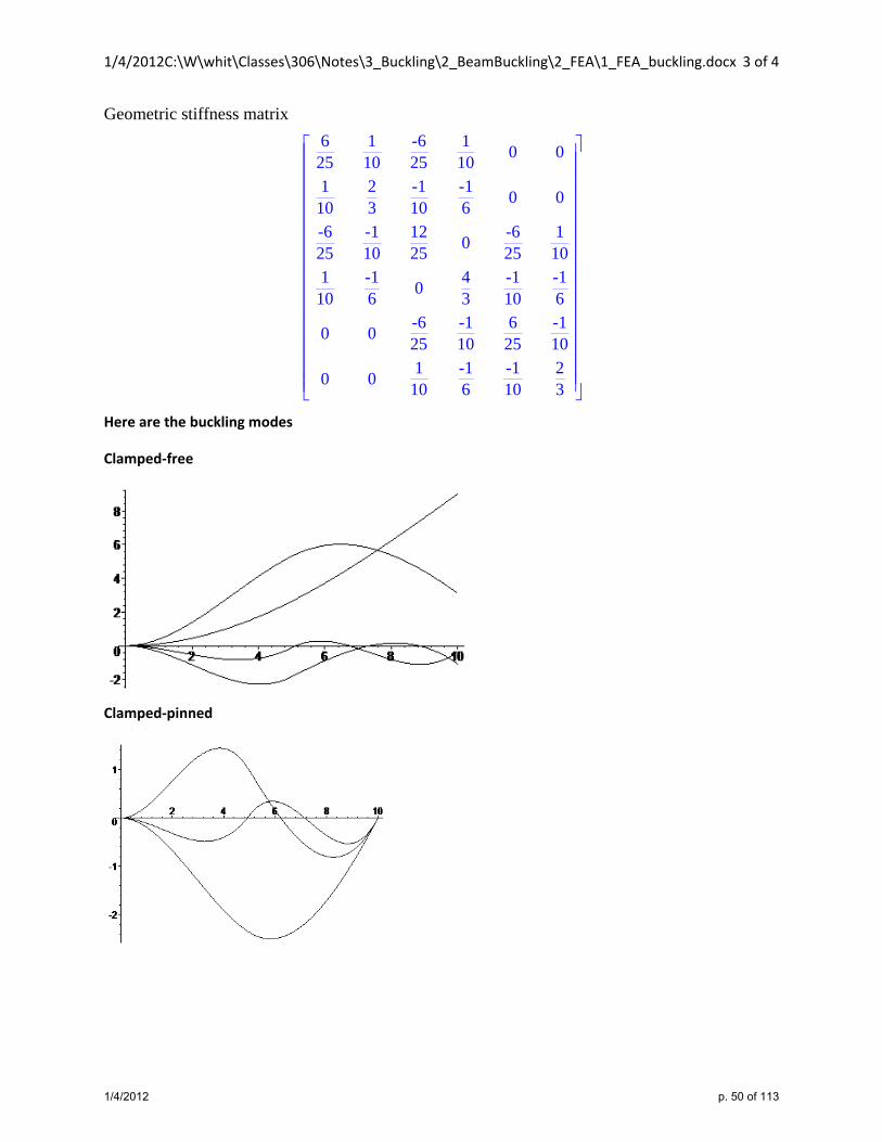
Geometric stiffness matrix
Here are the buckling modes
Clamped‐free
Clamped‐pinned
625
110
-625
110 0 0
110
23
-110
-16 0 0
-625
-110
1225 0 -6
251
101
10-16 0 4
3-110
-16
0 0 -625
-110
625
-110
0 0 110
-16
-110
23
1/4/2012 p. 50 of 113

1/4/2012C:\W\whit\Classes\306\Notes\3_Buckling\2_BeamBuckling\2_FEA\1_FEA_buckling.docx 4 of 4
Pinned‐pinned
Clamped‐clamped
Details are in the file beamBuckle_FEA.mws
1/4/2012 p. 51 of 113
C:\W\whit\Classes\306\Notes\3_Buckling\3_FrameBuckling\1_frame_Beambuckling_v2.doc Deepak Goyal p. 1 of 14
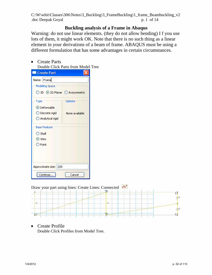
Buckling analysis of a Frame in Abaqus Warning: do not use linear elements. (they do not allow bending) I f you use lots of them, it might work OK. Note that there is no such thing as a linear element in your derivations of a beam of frame. ABAQUS must be using a different formulation that has some advantages in certain circumstances. • Create Parts
Double Click Parts from Model Tree
Draw your part using lines: Create Lines: Connected
• Create Profile
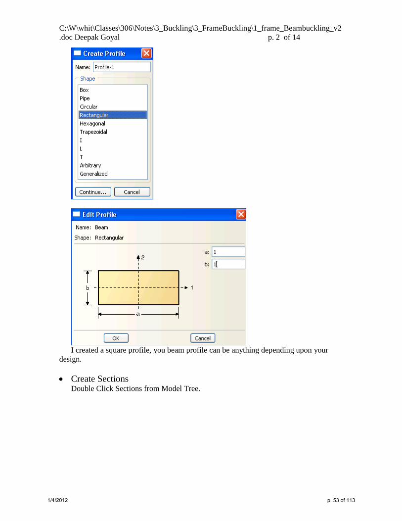
Double Click Profiles from Model Tree.
1/4/2012 p. 52 of 113
C:\W\whit\Classes\306\Notes\3_Buckling\3_FrameBuckling\1_frame_Beambuckling_v2.doc Deepak Goyal p. 2 of 14
I created a square profile, you beam profile can be anything depending upon your
design.
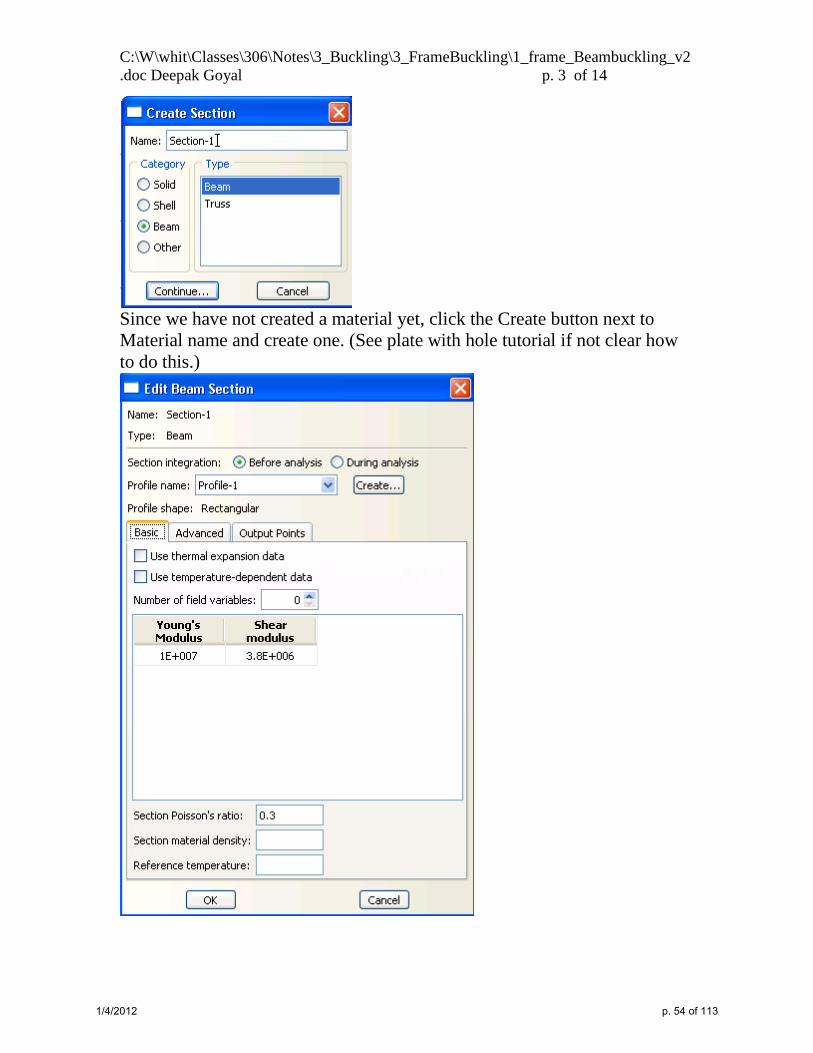
• Create Sections Double Click Sections from Model Tree.
1/4/2012 p. 53 of 113
C:\W\whit\Classes\306\Notes\3_Buckling\3_FrameBuckling\1_frame_Beambuckling_v2.doc Deepak Goyal p. 3 of 14
Since we have not created a material yet, click the Create button next to Material name and create one. (See plate with hole tutorial if not clear how to do this.)
1/4/2012 p. 54 of 113

C:\W\whit\Classes\306\Notes\3_Buckling\3_FrameBuckling\1_frame_Beambuckling_v2.doc Deepak Goyal p. 4 of 14
• Assign sections Open the part by clicking on the + on the part that we created. Double Click the “section Assignments icon”.
Select the regions to be assigned a section: here select the whole part using rectangular drag tool: All the part will become red after selection.
• Assign beam section orientations. Top toolbar (When Property Module
is loaded)
select the whole part and then click done: and put (0,0,-1) for approximate n1 direction.
1/4/2012 p. 55 of 113

C:\W\whit\Classes\306\Notes\3_Buckling\3_FrameBuckling\1_frame_Beambuckling_v2.doc Deepak Goyal p. 5 of 14
After you assign the direction, you get a plot like this (this particular plot is from another problem)
To get more information about what this means, go to the documentation: “12.13.3 Assigning a beam orientation” • Assembly
Open Assembly from Model Tree and double click on instances to create an instance.
• Mesh
Open the mesh module or select the mesh from the instance.
1/4/2012 p. 56 of 113

C:\W\whit\Classes\306\Notes\3_Buckling\3_FrameBuckling\1_frame_Beambuckling_v2.doc Deepak Goyal p. 6 of 14
• seed
click on seed part instance and select the whole part select a global size and click OK. Make the size large enough that you only get one element per member.
The seeding shown is actually more than is typically needed. • Assign element type
• create mesh
1/4/2012 p. 57 of 113

C:\W\whit\Classes\306\Notes\3_Buckling\3_FrameBuckling\1_frame_Beambuckling_v2.doc Deepak Goyal p. 7 of 14
Click “mesh part instance”, select the instance and say Yes. Abaqus will mesh the part: You will not see the mesh, but a message appears in the message window saying: 73 elements have been generated on instance: Part-1-1
• Create step
Double Click Steps from Model Tree.
Let’s specify 6 eigenvalues.
1/4/2012 p. 58 of 113

C:\W\whit\Classes\306\Notes\3_Buckling\3_FrameBuckling\1_frame_Beambuckling_v2.doc Deepak Goyal p. 8 of 14
• BC (in step-1) Expand step-1 and Double Click BCs from Model Tree.
Select region to be constrained
1/4/2012 p. 59 of 113

C:\W\whit\Classes\306\Notes\3_Buckling\3_FrameBuckling\1_frame_Beambuckling_v2.doc Deepak Goyal p. 9 of 14
you will see symbols
• Create Load Open Step1 (by clicking on the + sign) and Double Click Loads.
1/4/2012 p. 60 of 113

C:\W\whit\Classes\306\Notes\3_Buckling\3_FrameBuckling\1_frame_Beambuckling_v2.doc Deepak Goyal p. 10 of 14
select the nodes where you want to apply load.
you will see arrows appearing for loads.
1/4/2012 p. 61 of 113
C:\W\whit\Classes\306\Notes\3_Buckling\3_FrameBuckling\1_frame_Beambuckling_v2.doc Deepak Goyal p. 11 of 14
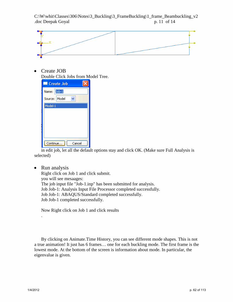
• Create JOB
Double Click Jobs from Model Tree.
in edit job, let all the default options stay and click OK. (Make sure Full Analysis is
selected) • Run analysis
Right click on Job 1 and click submit. you will see mesaages: The job input file "Job-1.inp" has been submitted for analysis. Job Job-1: Analysis Input File Processor completed successfully. Job Job-1: ABAQUS/Standard completed successfully. Job Job-1 completed successfully. Now Right click on Job 1 and click results . By clicking on Animate.Time History, you can see different mode shapes. This is not
a true animation! It just has 6 frames… one for each buckling mode. The first frame is the lowest mode. At the bottom of the screen is information about mode. In particular, the eigenvalue is given.
1/4/2012 p. 62 of 113

C:\W\whit\Classes\306\Notes\3_Buckling\3_FrameBuckling\1_frame_Beambuckling_v2.doc Deepak Goyal p. 12 of 14
1/4/2012 p. 63 of 113

C:\W\whit\Classes\306\Notes\3_Buckling\3_FrameBuckling\1_frame_Beambuckling_v2.doc Deepak Goyal p. 13 of 14
1/4/2012 p. 64 of 113

C:\W\whit\Classes\306\Notes\3_Buckling\3_FrameBuckling\1_frame_Beambuckling_v2.doc Deepak Goyal p. 14 of 14
1/4/2012 p. 65 of 113

C:\W\whit\Classes\306\Notes\3_Buckling\3_FrameBuckling\2_frameBuckling_summary.docx p. 1
Buckling of a Frame
Instructions for performing buckling analysis of a frame are given the file frame_Beambuckling_v2.doc.
If you use a single linear order element for each member, the predictions are very bad. The results are shown in the file frameBuckling_summary_coarse_linearElements.docx
Fixed on left side and loaded in compression on right side.
Options.Common to thicken the lines
Eigenvalues
1/4/2012 p. 66 of 113

C:\W\whit\Classes\306\Notes\3_Buckling\3_FrameBuckling\2_frameBuckling_summary.docx p. 2
Eigenmodes
1/4/2012 p. 67 of 113

C:\W\whit\Classes\306\Notes\3_Buckling\3_FrameBuckling\2_frameBuckling_summary.docx p. 3
1/4/2012 p. 68 of 113
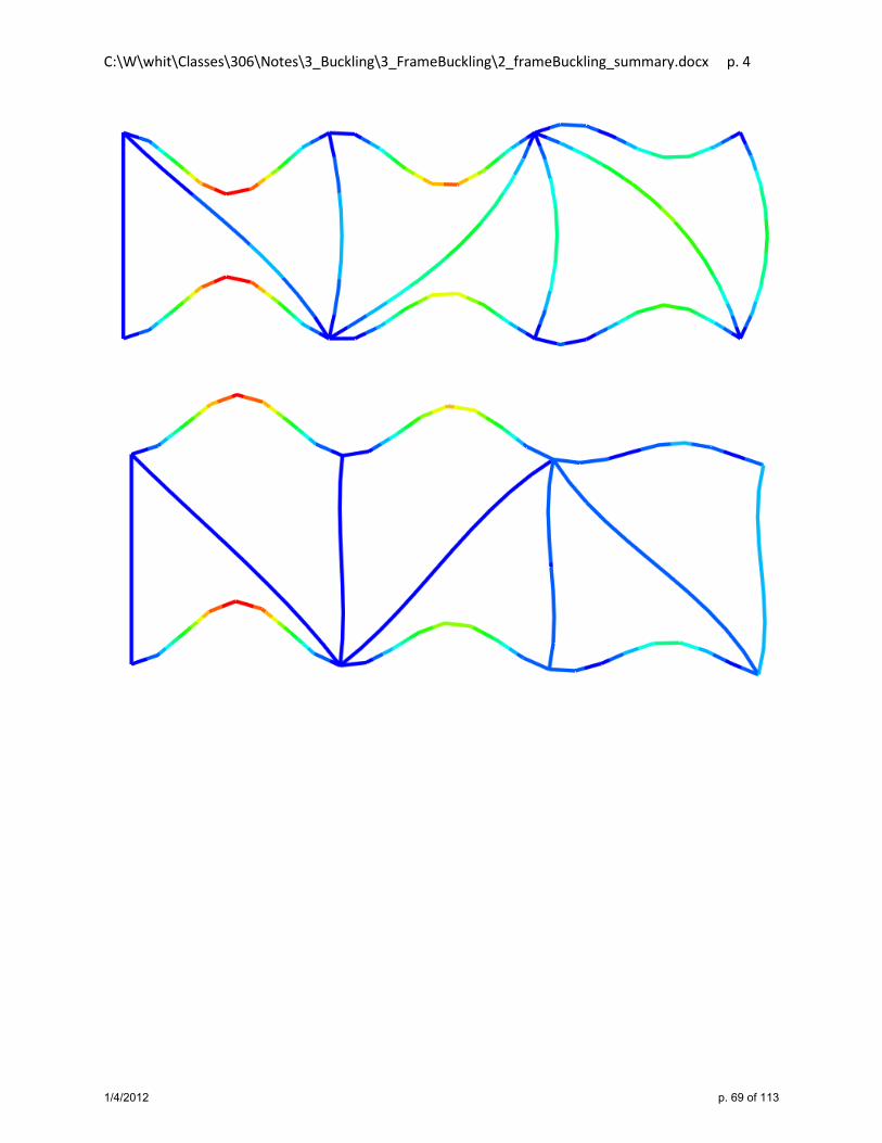
C:\W\whit\Classes\306\Notes\3_Buckling\3_FrameBuckling\2_frameBuckling_summary.docx p. 4
1/4/2012 p. 69 of 113

C:\W\whit\Classes\306\Notes\3_Buckling\3_FrameBuckling\3_frameBuckling_summary_coarse_linearElements.docx p. 1
Buckling of a Frame Truss?
Using a coarse mesh with the linear elements gives very bad predictions.
Options.Common
1/4/2012 p. 70 of 113

C:\W\whit\Classes\306\Notes\3_Buckling\3_FrameBuckling\3_frameBuckling_summary_coarse_linearElements.docx p. 2
1/4/2012 p. 71 of 113

C:\W\whit\Classes\306\Notes\3_Buckling\3_FrameBuckling\3_frameBuckling_summary_coarse_linearElements.docx p. 3
1/4/2012 p. 72 of 113

C:\W\whit\Classes\306\Notes\3_Buckling\3_FrameBuckling\3_frameBuckling_summary_coarse_linearElements.docx p. 4
1/4/2012 p. 73 of 113

C:\W\whit\Classes\306\Notes\3_Buckling\4_PlateBuckling\1_summary_Buckling_square_CAE_nice.docx
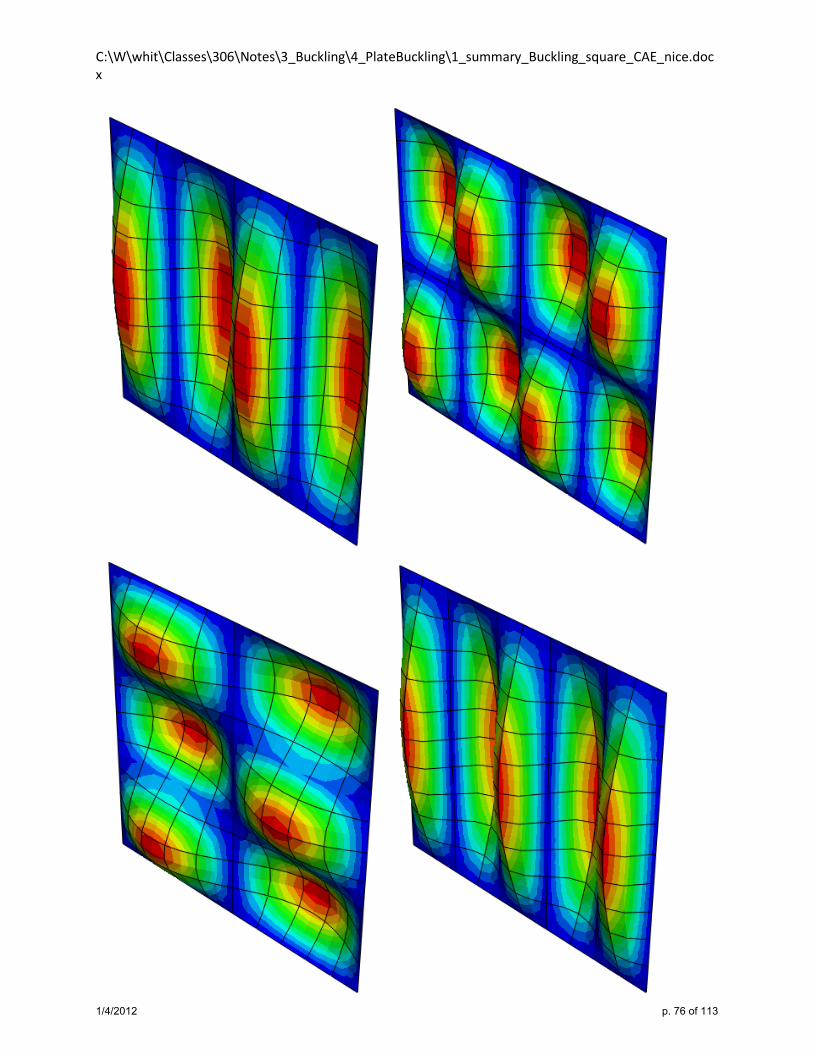
Buckling of a Square Plate under Compression
1/4/2012 p. 74 of 113

C:\W\whit\Classes\306\Notes\3_Buckling\4_PlateBuckling\1_summary_Buckling_square_CAE_nice.docx
1/4/2012 p. 75 of 113
C:\W\whit\Classes\306\Notes\3_Buckling\4_PlateBuckling\1_summary_Buckling_square_CAE_nice.docx
1/4/2012 p. 76 of 113
12/29/2011C:\W\whit\Classes\306\Notes\3_Buckling\4_PlateBuckling\2_plateBuckling_tutorial.docx 1 of 5
Analysis of Plate Buckling Using ABAQUS
1/4/2012 p. 77 of 113

12/29/2011C:\W\whit\Classes\306\Notes\3_Buckling\4_PlateBuckling\2_plateBuckling_tutorial.docx 2 of 5
PROBLEM DEFINITION:
Buckling of a plate.
PART:
3D->deformable->shell->Planar (size = 25)
sketch the part using rectangle tool, click done.
Dimensions of plate = 10x5
MATERIAL
create-name steel-mechanical-elasticity-elastic-isotropic.
E=200E9, nu = 0.3
SECTION
create->shell->homogenous.
shell thickness = 0.5
ASSIGN SECTION
Parts->Part1->section Assignments->select whole region->done->section1->OK->see color change.
ASSEMBLY
instances->dependent
1/4/2012 p. 78 of 113

12/29/2011C:\W\whit\Classes\306\Notes\3_Buckling\4_PlateBuckling\2_plateBuckling_tutorial.docx 3 of 5
STEPS
create step->step1->Type.Linear Perturbation ->buckle->continue->#ofeigenVals=5.
BCs
BC1:= Mechanical ->Disp/rotations -> continue -> select left edge->done ->clamp the end, u1, u2, u3, r1, r2, r3.
BC2:= Mechanical ->Disp/rotations -> continue -> select top edge->done -> u3=0, r1=0.
LOAD
create ->mechanical ->shell edge load ->continue ->select right edge ->done ->traction normal, magnitude = 10 -> OK
By end of it, you should have something like this.
1/4/2012 p. 79 of 113

12/29/2011C:\W\whit\Classes\306\Notes\3_Buckling\4_PlateBuckling\2_plateBuckling_tutorial.docx 4 of 5
MESH
part1->mesh->seed part->global size 0.5 ->OK->done->
from meshing toolbar assign element type -> geometric order quadratic, rest all defaults ->OK
from meshing toolbar ->Mesh part ->OK
JOB
create ->Full analysis (you can do data check and continue analysis also)
job1->submit
After Job Job-1 completed successfully,
right click Job1->results
USE THE BUTTONS WITH ARROWS
1/4/2012 p. 80 of 113

12/29/2011C:\W\whit\Classes\306\Notes\3_Buckling\4_PlateBuckling\2_plateBuckling_tutorial.docx 5 of 5
1/4/2012 p. 81 of 113

12/29/11 - C:\W\whit\Classes\306\Notes\3_Buckling\0_TotalPotentialEnergy\1_energyPrinciples.doc page 1of 10
Introduction to Buckling Analysis
Based on Total Potential Energy
1/4/2012 p. 82 of 113

12/29/11 - C:\W\whit\Classes\306\Notes\3_Buckling\0_TotalPotentialEnergy\1_energyPrinciples.doc page 2of 10
Variational and Energy Methods
Principle of Virtual Work Principle of Complementary Virtual Work Actual forces * virtual displacement Actual displacement * virtual forces Virtual displacement: satisfy kinematic constraints
Virtual forces: satisfy equilibrium equations and force type boundary conditions
Special cases: Minimum total potential energy Castigliano #1
Minimum total complementary energy Castigliano #2
Approximate solution Kinematic constraints satisfied exactly Equilibrium (interior and boundary)
satisfied exactly Equilibrium equations are derived (approximation satisfaction of equilibrium)
Compatibility equations are derived (approximation satisfaction of compatibility)
1/4/2012 p. 83 of 113
12/29/11 - C:\W\whit\Classes\306\Notes\3_Buckling\0_TotalPotentialEnergy\1_energyPrinciples.doc page 3of 10
Introduction to Energy Principles
Thus far we have constructed equilibrium equations two ways: using summation of forces =0 and virtual work=0. We will consider another way that is based on energy. In particular, we will use the Principle of Minimum Total Potential Energy. We will also mention an alternate way to express compatibility (i.e. kinematic) requirements using the Principle of Minimum Total Complementary Energy. These two principles can be stated as follows: (Allen & Haisler) Principle of Minimum Total Potential Energy: Of all the possible displacements that satisfy the boundary conditions of a deformable body or structural system, those corresponding to the stable equilibrium position make the total potential energy a relative minimum. If the first variation of the total potential energy is zero (also known as being “stationary”), but not at a relative minimum, the equilibrium configuration is not stable. We will discuss stability below. Principle of Minimum Total Complementary Energy: Of all the possible stresses and forces that satisfy the equilibrium conditions and stress boundary conditions of a deformable body or structural system, those corresponding to the true stable deformation state make the total complementary energy a relative minimum. (This principle is used to derive compatibility equations, not equilibrium equations.) The total potential energy consists of two parts: the potential of the applied loads (“V” … not to be confused with shear!) and the strain energy that is stored inside an elastic body (“U”). We will discuss how to calculate these very soon. Mathematically, we can express the requirement for finding a “stationary” value of total potential energy as setting the first variation of Π to zero, i.e. 0δ Π = . In general, we will be working to obtain approximate solutions that have been expressed in terms of a collection of unknown parameters. If we call these unknown parameters iq , then the requirement that the first variation be zero is given by
1 2 31 2 3
... 0q q qq q q
δ δ δ δ∂Π ∂Π ∂ΠΠ = + + + =
∂ ∂ ∂
To satisfy this requires that each partial derivative equal zero.
1 2 3
... 0q q q
∂Π ∂Π ∂Π= = = =
∂ ∂ ∂
Thus if there are n unknowns, we will obtain n simultaneous equations that we can use to solve for the unknowns. Example Consider a linear spring subjected to a force P. The resulting displacement is u.
Show that the strain energy in the spring, U = 212
ku .
1/4/2012 p. 84 of 113

12/29/11 - C:\W\whit\Classes\306\Notes\3_Buckling\0_TotalPotentialEnergy\1_energyPrinciples.doc page 4of 10
The potential of the applied load = - (force vector ) (displacement vector) . In other words, a force loses potential when it moves in the direction of the force. The amount of loss is simply the dot product of the force and displacement vectors. For our spring, the potential V= -Pu
Hence, 212
Pu kuΠ = − + . Setting 0δ Π = gives the familiar equilibrium equation P=ku.
Until now you have solved equilibrium equations and never worried about whether the equilibrium state was stable or unstable. In real structures this is a critical concern. The following sketch illustrates the concept of stability using a ball on a curved surface and gravity acting downward. The total potential energy Π = w y, where w= the weight of the ball and y= the height. All three balls are in equilibrium, but the stability is different. Imagine what would happen to each ball if it was perturbed slightly. (e.g. you hit each one with a small ball) The reaction is determined by the stability. This sketch illustrates “stable”, “unstable”, and “conditional or neutral” equilibrium.
Comments
• strain energy of a linear spring, U = 212
ku
• potential of applied load = - (force vector ) (displacement vector) • change in potential is generally not equal to the work done by the force (only equal if the
force is constant during the motion) • What is the potential of a distributed load? • A force F is used to stretch a spring “b” inches. Assume the spring is non-linear with
force vs. displacement relationship of F = a u3, where a = a constant. o How much work is done by the force? o What is potential of the force at equilibrium? Assume the potential is zero before
the spring begins to stretch.
Π
F,b
1/4/2012 p. 85 of 113

12/29/11 - C:\W\whit\Classes\306\Notes\3_Buckling\0_TotalPotentialEnergy\1_energyPrinciples.doc page 5of 10
Summary of Terms (no thermal effects)
The following assume nonlinear elastic behavior. Internal
δε
F
Uo
′Uo
δF
ε
Fδε
εδF ε, Fc h
External
P P uδ
u Pδ u P,c h
u
1/4/2012 p. 86 of 113

12/29/11 - C:\W\whit\Classes\306\Notes\3_Buckling\0_TotalPotentialEnergy\1_energyPrinciples.doc page 6of 10
Total Potential Energy for a Spring Let’s look at total potential energy for a linear spring. The work done on the spring = strain
energy stored in the spring, since there is no dissipation.
This plot below shows how the strain energy U, the potential of the applied load V, and the total
potential energy U+V vary with u.
• The strain energy, U, increases monotonically. • The potential of applied load, V, decreases monotonically • The total potential energy, U+V, decreases and then increases. There is a location where
U+V has a minimum value, which can be calculated by setting
0 (for this problem, this is equivalent to 0)u
δ ∂ΠΠ = =
∂. Calculate the minimum point and
compare it to the plot. (Plot is from the file springEnergy.mws)
1/4/2012 p. 87 of 113

12/29/11 - C:\W\whit\Classes\306\Notes\3_Buckling\0_TotalPotentialEnergy\1_energyPrinciples.doc page 7of 10
Strain Energy for a Linear Elastic Bar For an elastic body, the work done by the forces that deform the body = the energy stored by the body. This is because there is no dissipation of energy. We will calculate the work of the applied loads… and then we will know the strain energy in the body. The work done by the forces on the differential element is (why the ½?)
( )( )
[ ]
12 212 21 (High order terms are dropped.)2
dudW Fu F dF u du fdx u
fFu Fu Fdu udF dFdu fudx dxdu
Fdu udF fudx
= − + + + + + = − + + + + + +
= + +
Now let’s determine the work for the entire bar. We need to add up the differential work for all
of the differential elements. We need to integrate. 2
1
final
initial
W x
W x
dWdW dxdx
=∫ ∫
1 1 12 2 2
dW du dF du dF duF u fu F u f Fdx dx dx dx dx dx
= + + = + + = Why?
2
1
1 strain energy2
x
x
duW F dx Udx
∴ = = ≡∫
To use this we will need to express F in terms of displacement, which gives 2
0
12
L duU EA dxdx
= ∫
Comment
(which is equal to ), is referred to as the strain energy density for a uniaxial bar.dU dWdx dx
Modification for thermal load There is more than one way to include thermal effects. Two possibilities are
21 22
du duU EA T dxdx dx
α = − ∆
∫ and 2
0
12
L duU EA T dxdx
α = − ∆ ∫
At first, one might expect a problem, since these are obviously different formulas. However, there is no practical difference, since the typical use of “U” is in determining the equilibrium requirements by minimizing total potential energy. Although the formulas for U are different,
Uδ obtained from the two formulas is the same. Try it! Hint: ( ) 0Tδ α∆ =
F, u
F + dF u + du
f
dx
1/4/2012 p. 88 of 113

12/29/11 - C:\W\whit\Classes\306\Notes\3_Buckling\0_TotalPotentialEnergy\1_energyPrinciples.doc page 8of 10
Derivation of 21 2
2du duU EA T dxdx dx
α = − ∆
∫
This is a little tricky. See file strainEnergy_thermal.mws
Derivation of 2
0
12
L duU EA T dxdx
α = − ∆ ∫
In this case, we take the viewpoint that free thermal expansion strains cause no strain energy.
Hence, we simply substitute du Tdx
α− ∆ for the dudx
in the formula 2
0
12
L duU EA dxdx
= ∫ .
Immediately, we have the desired formula. Personally, I prefer this second formula. Consider the case of a uniaxial bar that is prevented
form moving at both ends and then heated. The strain dudx
is zero, but I can assure you that if the
thermal expansion coefficient is not zero, there is plenty of energy stored in the bar. The first formula would give zero energy. Equivalence of Principle of Virtual Work and Principle of Minimum Total Potential Energy When Π exists (which it does for any system we will consider), the equations obtained using virtual work and minimum total potential energy are identical. Since we have already studied virtual work in detail, there is no need to repeat the effort here. The equivalence is illustrated below for a uniaxial bar problem.
F u L, b g
f
( )
( ) ( )
vol 0
vol 0 vol 0
12
0 0
...this is identical to the VW equation if we multiply through by -1!
L
L
L L
L L
E dV Fu pudx
E dV F u p udx dV F u p udx
ε
δ εδε δ δ σδε δ δ
Π = − −
=> Π = = − − = − − =
∫ ∫
∫ ∫ ∫ ∫
This is not the case for uniaxial bars only… it is always the case. If you can write the total potential energy, then the setting the variation of the total potential energy to zero will result in the virtual work equation. Inverse method of derivation
• Start with the virtual work equation. • Use the properties of variational operator “δ ” to identify what you would take the
variation of to obtain the virtual work equation. • Re-write the virtual work as ( ) 0δ =
1/4/2012 p. 89 of 113
12/29/11 - C:\W\whit\Classes\306\Notes\3_Buckling\0_TotalPotentialEnergy\1_energyPrinciples.doc page 9of 10
• Identify part of what is in the parentheses as the internal energy (strain energy) and part as the potential of the applied loads.
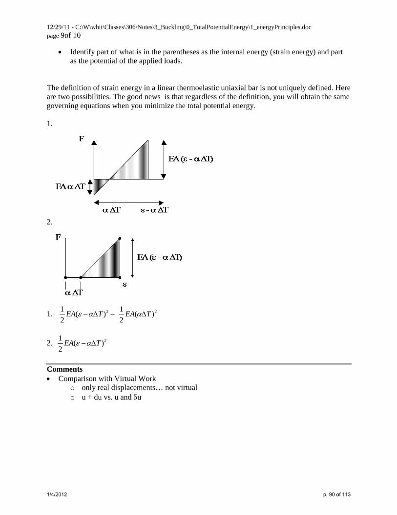
The definition of strain energy in a linear thermoelastic uniaxial bar is not uniquely defined. Here are two possibilities. The good news is that regardless of the definition, you will obtain the same governing equations when you minimize the total potential energy. 1.
2.
1. 2 21 1( ) ( )
2 2EA T EA Tε α α− ∆ − ∆
2. 21 ( )2
EA Tε α− ∆
Comments • Comparison with Virtual Work
o only real displacements… not virtual o u + du vs. u and δu
1/4/2012 p. 90 of 113

12/29/11 - C:\W\whit\Classes\306\Notes\3_Buckling\0_TotalPotentialEnergy\1_energyPrinciples.doc page 10of 10
Strain Energy for a Beam • Assume linear elasticity f
V
M + dM M
V + dV v + dv θ + dθ
v, θ
( ) ( ) ( ) ( ) ( )
( )
2 work2
2
dvd M M dM d Vv V dV v dv fdx v
M M Md dM dMd Vv Vv Vdv vdV dVdv fdxvd MdW dVv fv
dx dx dx
θ θ θ
θ θ θ θ θθ
× = − + + + − + + + + +
= − + + + + − + + + + +
× = + +
( ) ( )d MTherefore 2 * work =
d Vvfv dx
dx dx
dM d dV dvM v V fv dxdx dx dx dx
θ
θθ
+ +
= + + + +
∫
∫
But dMdx
V dvdx
= − = and θ
( )dv d dV dvV M v V fv dx
dx dx dx dxd dVM v f dxdx dx
θ
θ
= − + + + + = + +
∫
∫
22
2
1 12 2
U W
d d vU M dx EI dxdx dxθ
=
⇒ = =
∫ ∫
We will not consider strain energy for a beam with thermal loads (lack of time)
1/4/2012 p. 91 of 113

C:\W\whit\Classes\306\Notes\3_Buckling\0_TotalPotentialEnergy\2_buckling_intro.doc page 1 of 7
Introduction to Buckling of Structures
Why are we interested in buckling ? In most structures the displacements increase gradually with increased applied load. If the
applied load is too large (particularly for compressive structures), a small increase in applied load can lead to a sudden large increase in the displacements. Buckling refers to this transition to large, often catastrophic displacements. Buckling can occur due to thermal or mechanical loads. Sometimes this abrupt behavior can be exploited for useful purposes.
Buckling is one type of instability. Instability is a state in which small perturbations (e.g. small increments in load) can cause large changes in the response of the structure. Instability can be due to geometric effects (as is usually the case in buckling) or change in material properties. (e.g. material yielding or failure) Instability occurs in a variety of physical systems other than structures, such as those involving heat transfer and fluid flow. In this course we will limit ourselves to instability of structures due buckling. Examples of buckling
• collapse of yardstick due to excess axial load • collapse of assemblage of white-board markers due to excess axial load • buckling of roads on hot days • collapse of large towers (comprised of trusses and stay wires) • bi-metallic strip used for thermostat • truss bridges • collapse of thin shell (Coke can) • etc.
The onset of buckling (instability) is based on total potential energy. • The requirement for equilibrium is δ Π =0 , where Π is the total potential energy.
It is easily shown that this is equivalent to setting the virtual work to zero. • Stability of the equilibrium state depends on whether Π increases or decreases
with small perturbation of displacements. • Total potential energy consists of two parts. The first part is the potential energy due
to location. In particular, a force, F, loses potential when it moves through some distance, u. The amount of loss = F u , the maximum amount of work the force could have done. It is essential to realize that the loss of potential is not related to the body the force is imposed on. It is strictly a geometric concern. If we take the potential of a force to be zero before moving the force, then the potential of the force = -F u. The other component of total potential energy is internal energy, which is in the form of strain energy. The strain energy in an elastic body can be determined by determining the amount of work that is done on the body by forces. For a linear elastic
spring, it is easy to show that this work is 12
2k u , where k = the spring constant and u
= the stretch or compression of the spring.
1/4/2012 p. 92 of 113
C:\W\whit\Classes\306\Notes\3_Buckling\0_TotalPotentialEnergy\2_buckling_intro.doc page 2 of 7
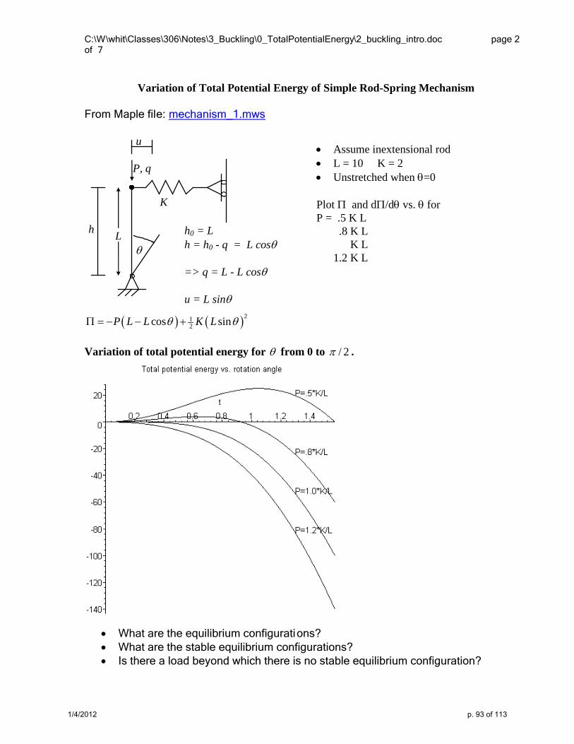
Variation of Total Potential Energy of Simple Rod-Spring Mechanism
From Maple file: mechanism_1.mws
P, q
K
θ
u
L h h0 = L h = h0 - q = L cosθ => q = L - L cosθ u = L sinθ
• Assume inextensional rod • L = 10 K = 2 • Unstretched when θ=0 Plot Π and dΠ/dθ vs. θ for P = .5 K L .8 K L K L 1.2 K L
( ) ( )21
2cos sinP L L K Lθ θΠ = − − + Variation of total potential energy for θ from 0 to / 2π .
• What are the equilibrium configurations? • What are the stable equilibrium configurations? • Is there a load beyond which there is no stable equilibrium configuration?
1/4/2012 p. 93 of 113

C:\W\whit\Classes\306\Notes\3_Buckling\0_TotalPotentialEnergy\2_buckling_intro.doc page 3 of 7
We can answer the first question, but the others require a careful look at the what happens to the total potential energy when a system is perturbed from an equilibrium state. We will do this using a Taylor series expansion. The next section describes how a Taylor series can be used… then we will come back and consider the behavior of the mechanism in greater detail.
Taylor Series about Equilibrium Position Stability is determined by how Total Potential Energy changes when position changes slightly. Single dof
( ) ( ) ( ) ( )( ) ( )( )2 3
2 32 3
1 1 ...2! 3!
d d dq q q q q q q q qdq dq dq
δ δ δ δΠ Π ΠΠ + = Π + + + +
( ) ( )
( ) ( )2 3
2 32 3
1 12! 3!
q q q
d d dq q qdq dq dq
δ
δ δ δ
∆Π = Π + −Π
Π Π Π= + + +
2
2
2
2
2
2
2
2
: 0at equilibrium => sign of depends on sign of
d 0 stable
d 0 unstable
d 0 neutral or conditional stability
examine higher order terms (ie. derivatives)
d dNotedq dq
dq
dq
dq
Π Π= ∆Π
Π> ⇒
Π< ⇒
Π= ⇒
⇒
Note: 2
2
ddqΠ
= tangent stiffness
Multiple-dof: Determinant & Eigenvalues
The incremental stiffness for a multi -dof problem is given by2
iji j
Kq q∂∂ ∂
Π= . When the load
becomes large enough to cause buckling, the displacements can increase without a change in the loads, i.e. 0K q∆ = . This has non-trivial solutions only if K =0. Hence, we
solve K =0 to determine the critical loads. This problem can be cast as an
1/4/2012 p. 94 of 113

C:\W\whit\Classes\306\Notes\3_Buckling\0_TotalPotentialEnergy\2_buckling_intro.doc page 4 of 7
eigenvalue problem. Using this technique we can obtain the critical loads and the buckled shape. The eigenvalue problem is set up as follows. K will consist of two parts… one part that is independent of the applied loads and another that is linearly related to the applied loads. We will call these 0K and Kσ , often referred to as the linear and geometric stiffness matrices. Hence,
0K K Kσ= + Now let’s assume that we impose some loads on the structure and then calculate Kσ for those loads. It is doubtful that we would have specified just the right load level to cause buckling. We would expect to have to scale the load up or down. Since Kσ varies linearly with the applied load, the Kσ at buckling would be Kσλ , λ is the scale factor required. Hence, we are searching for the value of λ that satisfies ( )0
10 0
10
0Rearranging we obtain
The standard eigenvalue problem is Ax = x, where are the eigenvalues. Therefore, if the applied loads are scaled by -(eigenvalues of )
K K q
K q K q K K q q
K K
σ
σ σ
σ
λ
λ λλ λ
−
−
+ ∆ =
∆ = − ∆ => ∆ = − ∆
, the critical loadsare obtained. The buckling shapes are given by the eigenvectors.
You should learn how to determine the critical load using both techniques ( 0K = and setting up an eigenvalue problem. The first technique is only useful for very small problems. When there are more than a few roots, we are finding the roots of a high order polynomial… and will easily run int o numerical difficulties. Further thoughts
• Show that 2
2
ddqΠ
gives the stiffness for a spring that is fixed on one end.
• Show that the beam stiffness matrix can be determined from2
iji j
Kq q∂∂ ∂
Π= .
1/4/2012 p. 95 of 113
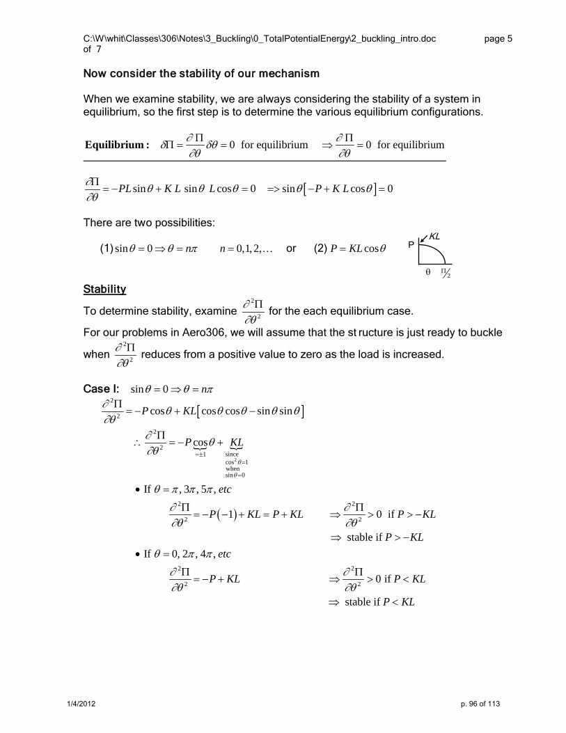
C:\W\whit\Classes\306\Notes\3_Buckling\0_TotalPotentialEnergy\2_buckling_intro.doc page 5 of 7
Now consider the stability of our mechanism When we examine stability, we are always considering the stability of a system in equilibrium, so the first step is to determine the various equilibrium configurations.
0 for equilibrium 0 for equilibrium∂ ∂δ δθ∂θ ∂θΠ Π
Π = = ⇒ =Equilibrium :
[ ]sin sin cos 0 sin cos 0PL K L L P K L∂ θ θ θ θ θ∂θΠ
= − + = => − + =
There are two possibilities:
(1) sin 0 0,1,2,n nθ θ π= ⇒ = = or (2) cosP KL θ= Stability
To determine stability, examine 2
2
∂∂θΠ
for the each equilibrium case.
For our problems in Aero306, we will assume that the st ructure is just ready to buckle
when 2
2
∂∂θΠ
reduces from a positive value to zero as the load is increased.
Case I: sin 0 nθ θ π= ⇒ =
[ ]
( )
2
2
2
2
2since1cos 1whensin 0
2 2
2 2
2 2
2 2
cos cos cos sin sin
cos
If , 3 , 5 ,
1 0 if
stable if If 0, 2 , 4 ,
0 if
sta
P KL
P KL
etc
P KL P KL P KL
P KLetc
P KL P KL
θ
θ
∂ θ θ θ θ θ∂θ
∂ θ∂θ
θ π π π
∂ ∂∂θ ∂θ
θ π π
∂ ∂∂θ ∂θ
=±=
=
Π= − + −
Π∴ = − +
• =
Π Π= − − + = + ⇒ > > −
⇒ > −• =
Π Π= − + ⇒ > <
⇒ ble if P KL<
KL
θ Π2
P
1/4/2012 p. 96 of 113
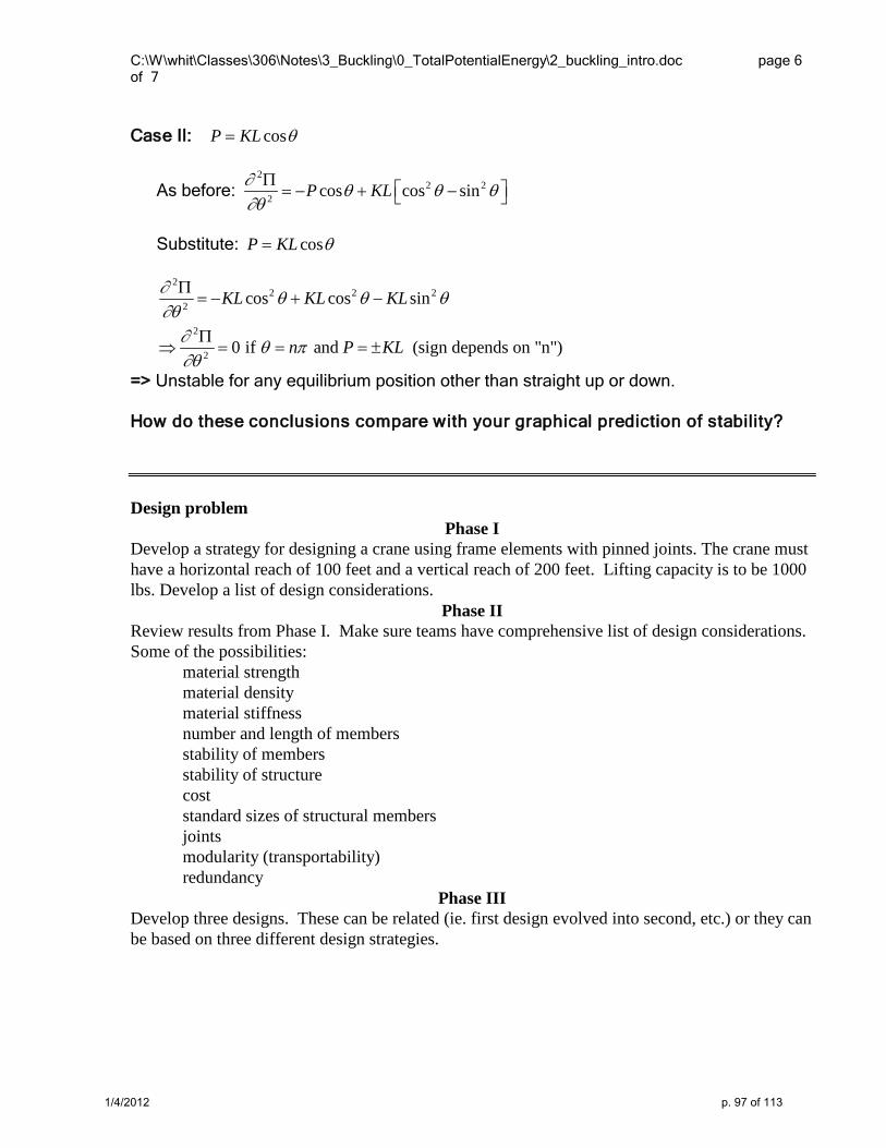
C:\W\whit\Classes\306\Notes\3_Buckling\0_TotalPotentialEnergy\2_buckling_intro.doc page 6 of 7
Case II: cosP KL θ=
As before: 2
2 22 cos cos sinP KL∂ θ θ θ
∂θΠ = − + −
Substitute: cosP KL θ=
22 2 2
2
2
2
cos cos sin
0 if and (sign depends on "n")
KL KL KL
n P KL
∂ θ θ θ∂θ∂ θ π∂θ
Π= − + −
Π⇒ = = = ±
=> Unstable for any equilibrium position other than straight up or down. How do these conclusions compare with your graphical prediction of stability? Design problem
Phase I Develop a strategy for designing a crane using frame elements with pinned joints. The crane must have a horizontal reach of 100 feet and a vertical reach of 200 feet. Lifting capacity is to be 1000 lbs. Develop a list of design considerations.
Phase II Review results from Phase I. Make sure teams have comprehensive list of design considerations. Some of the possibilities: material strength material density material stiffness number and length of members stability of members stability of structure cost standard sizes of structural members joints modularity (transportability) redundancy
Phase III Develop three designs. These can be related (ie. first design evolved into second, etc.) or they can be based on three different design strategies.
1/4/2012 p. 97 of 113

C:\W\whit\Classes\306\Notes\3_Buckling\0_TotalPotentialEnergy\2_buckling_intro.doc page 7 of 7
1/4/2012 p. 98 of 113

(1)(1)
> >
> >
Buckling Loads and Modes
3_5_30_smallAngleApprox.mws
det(K)=0 and eigenvalue technique
5.30 Allen & Haisler
Assume the springs are undeformed when the rods are vertical.
restart:with(linalg):currentdir();
"C:\Users\whit\Desktop\Active"
Calculate total potential energyMake small angle approximations: sin(angle) = angle cos(angle) = 1- 1/2 * angle^2This implicitly assumes that we are considering instability from a vertical orientation.What if we do not make this approximation at the beginning? See the file 5b_5_30_eigen.mws.sin_t1 := theta[1]:sin_t2 := theta[2]:cos_t1 := 1-theta[1]^2/2:cos_t2 := 1-theta[2]^2/2:
1/4/2012 p. 99 of 113

> >
(2.1)(2.1)
(2.2)(2.2)> >
(1.2)(1.2)
(1.1)(1.1)
> >
L1 := L/2:L2 := L/2:u := L1*sin_t1 + L2*sin_t2;
u := 12
L θ1C12
L θ2
EnergyAssumes positive displacement is up and V is zero when bars are horizontal. (One can also choose another reference state... we will get the same answer.)U := 1/2 * K1 * u^2 + 1/2 * K2 *(theta[1]-theta[2])^2;V := -(-P)*(L1 * cos_t1 +L2*cos_t2 );PI := U+V;
U := 12
K1 12
L θ1C12
L θ2
2C
12
K2 θ1Kθ22
V := P 12
L 1K 12
θ12
C12
L 1K 12
θ22
Π := 12
K1 12
L θ1C12
L θ2
2C
12
K2 θ1Kθ22CP 1
2 L 1K 1
2 θ1
2C
12
L 1
K12
θ22
Calculation of critical load using det(K)=0 at equilibrium stateLet's determine the buckling load if the pre-buckling configuration is theta[1]=theta[2]=0. We should verify that this corresponds to an equilibrium state. We do this by showing that these angles satisfy
v
vtheta1 PI = 0
v
vtheta2 PI = 0
eqns := [diff(PI,theta[1]),diff(PI,theta[2])] ;
eqns := 12
K1 12
L θ1C12
L θ2 LCK2 θ1Kθ2 K12
P L θ1,12
K1 12
L θ1
C12
L θ2 LKK2 θ1Kθ2 K12
P L θ2
Check for equilibrium for the condition that both angles are zero. subs(theta[1]=0, theta[2]=0,eqns);
0, 0
Now let's determine the critical load by solving
det
v2
vq12 PI v2
vq2 vq1 PI
v2
vq1 vq2 PI v2
vq22 PI
=0
1/4/2012 p. 100 of 113

> >
> >
(3.1.1)(3.1.1)
(2.4)(2.4)
> >
> >
(3.1.3)(3.1.3)
> >
(2.3)(2.3)
(3.1.2)(3.1.2)
Calculate the stiffness matrixq:= [theta[1], theta[2]]:K := array(1..2,1..2):for i from 1 to 2 dofor j from 1 to 2 doK[i,j] := diff(PI,q[i], q[j]);od:od:evalm(K);
K1 L2
4CK2K
P L2
K1 L2
4KK2
K1 L2
4KK2
K1 L2
4CK2K
P L2
Determine the critical loads by solving det(K)=0ans:=solve(det(K)=0, P);
ans := 4 K2L
, K1 L
Calculation of mode shapes (getting the eigenvectors)Recall that we were solving to obtain non-trivial solutions.
First modeSubstitute the first eigenvalue into the matrix K and define the resulting matrix to be KKKK := map( proc(zz) subs(P=ans[1],zz) end, evalm(K) );
KK :=
K1 L2
4KK2
K1 L2
4KK2
K1 L2
4KK2
K1 L2
4KK2
We need to specify the magnitude of one of the components of the eigenvector. (otherwise, there is an infinite number of solutions)Assume that theta[1] = 1 and then determine theta[2]r:=evalm( KK &* [1, theta[2] ]);
r := K1 L2
4KK2C
K1 L2
4KK2 θ2
K1 L2
4KK2C
K1 L2
4KK2 θ2
I now have two equations... r[1] =0 and r[2] =0. We can choose either one to solve for theta[2].solve( r[1]=0, theta[2] );solve( r[2]=0, theta[2] );
K1K1
Hence, the first eigenvector (mode) is (1,1). What does this mean?
1/4/2012 p. 101 of 113

> >
(3.2.1)(3.2.1)
> >
I could have assumed that theta[2] = 1 and solved for theta[1]. The result would be the same.Important This procedure gives the mode shape, not the magnitude of the displacements.
Second modeRepeat the process process for the second mode. Now we use the second eigenvalue.KK := map( proc(zz) subs(P=ans[2],zz) end, evalm(K) );r:=evalm( KK &* [1, theta[2] ]);solve( r[1]=0, theta[2] );
KK :=K
K1 L2
4CK2
K1 L2
4KK2
K1 L2
4KK2 K
K1 L2
4CK2
r := KK1 L2
4CK2C
K1 L2
4KK2 θ2
K1 L2
4KK2C K
K1 L2
4CK2 θ2
1
This shows that the second mode is (1,-1).
Calculation of critical load and buckling shape using "standard" eigenvalue analysis
Note: K0 is the linear stiffness matrix. It does not depend on the applied load. Ksigma is the geometric stiffness matrix. It does depend on the applied load.We calculated the total stiffness matrix earlier... and called it "K". Now let's split the matrix into two matrices: the linear and geometric stiffness matrices.The linear stiffness matrix does not depend on the load, so if we substitute P=0 into K, we will extract the linear stiffness matrix.K0 := array(1..2,1..2):for i from 1 to 2 dofor j from 1 to 2 doK0[i,j] := subs(P=0, K[i,j] ):
1/4/2012 p. 102 of 113

> >
(2)(2)
> >
(4.1)(4.1)
> >
(4.2)(4.2)
(3)(3)
od:od:evalm(K0);
K1 L2
4CK2
K1 L2
4KK2
K1 L2
4KK2
K1 L2
4CK2
Since the sum of the linear and geometric stiffness matrix = second derivative, simply subtract the linear stiffness matrix to get the geometric stiffness matrix.Ksigma := evalm( K-K0);
This is not the usual way to calculate the linear and geometric stiffness matrices, but given what we have covered thus far, it is the way to do it. When we get to buckling of beams, we will derive a better way.
Ksigma :=K
P L2
0
0 KP L2
Now let's solve the eigenvalue problem
Kmod := evalm(inverse(Ksigma) &* K0);
Kmod :=K
2 K1 L2
4CK2
P LK
2 K1 L2
4KK2
P L
K2 K1 L2
4KK2
P LK
2 K1 L2
4CK2
P L
Calculate the eigenvalueseigenvals(Kmod);
K4 K2P L
, KK1 LP
According to the formula above, we obtain the critical load by multiplying the applied load by the
negative of the eigenvalues. Thus the critical loads are 4 K2L
, K1 L
We can also determine the buckling modes.
1/4/2012 p. 103 of 113

(4)(4)
(5)(5)
> >
result:=eigenvects(Kmod);
result := K4 K2P L
, 1, K1 1 , KK1 L
P, 1, 1 1
The syntax is a bit cumbersome for the result returned by the function eigenvects. Note that this function also calculates the eigenvalues. The two modes areresult[1][3];result[2][3];
K1 1
1 1
This says that for one buckling mode the two angles are the same. (=> bars stay co-linear)For the other buckling mode the angles are the same magnitude, but opposite sign.
1/4/2012 p. 104 of 113

> >
> >
(1)(1)
(1.1)(1.1)
Buckling Loads and Modes
w/o using small angle approximation
4_5_30_eigen.mwSolved as an eigenvalue problem
5.30 Allen & Haisler
restart:with(linalg):currentdir();
"C:\W\whit\Classes\306\Notes\3_Buckling\0_TotalPotentialEnergy"
Calculate total potential energy For variety the input in this section is displayed in standard math notation. To see text you can edit, simply highlight the input, right click, and toggle off the Standard Math option.
L1 := L2
; L2 := L2
; u := L1 sin θ1 CL2 sin θ2 ; U := 1 K1 u2
2C
1 K2 θ2Kθ12
2; V :=
P L1 cos θ1 CL2 cos θ2 ;
Π := UCV
L1 := 12
L
L2 := 12
L
u := 12
L sin θ1 C12
L sin θ2
U := 12
K1 12
L sin θ1 C12
L sin θ2
2C
12
K2 θ2Kθ12
V := P 12
L cos θ1 C12
L cos θ2
Π := 12
K1 12
L sin θ1 C12
L sin θ2
2C
12
K2 θ2Kθ12CP 1
2 L cos θ1
C12
L cos θ2
Setting up the eigenvalue problem
1/4/2012 p. 105 of 113

(2.1)(2.1)
> >
(2.2)(2.2)
(2.3)(2.3)
> >
(2.4)(2.4)
> >
> >
> >
First we calculate Kij , the second derivative of the total potential energy.K := [ [ diff(PI,theta[1],theta[1]), diff(PI,theta[1],theta[2])], [ diff(PI,theta[2],theta[1]), diff(PI,theta[2],theta[2]) ] ];
K := 14
K1 L2 cos θ12K
12
K1 12
L sin θ1 C12
L sin θ2 L sin θ1 CK2
K12
P L cos θ1 , 14
K1 L2 cos θ2 cos θ1 KK2 , 14
K1 L2 cos θ2 cos θ1
KK2, 14
K1 L2 cos θ22K
12
K1 12
L sin θ1 C12
L sin θ2 L sin θ2 CK2
K12
P L cos θ2
Assume buckling occurs from a straight configuration. That is, assume the the pre-buckling equilibrium configuration has the two bars vertical. Imposing the equilibrium condition means that we substitute zero values for the angles. We can shorten what follows by writing a procedure for calculating K as a function of the angles and the load P.KK := unapply(K,P, theta[1], theta[2]):evalm(KK(P,0,0));
As you can see, there are terms that are independent of P and some that are linearly related to P.14
K1 L2CK2K12
P L 14
K1 L2KK2
14
K1 L2KK214
K1 L2CK2K12
P L
The linear stiffness matrix does not depend on the load, so if we substitute P=0 into second derivative, we will extract the linear stiffness matrix.K0 := evalm(KK(0,0,0));
K0 :=
14
K1 L2CK214
K1 L2KK2
14
K1 L2KK214
K1 L2CK2
Since the sum of the linear and geometric stiffness matrix = second derivative, simply subtract the linear stiffness matrix to get the geometric stiffness matrix.Ksigma := evalm( KK(P,0,0)-K0);
Ksigma :=K
12
P L 0
0 K12
P L
Let's assume Ksigma is to be calculated when P=1. Then the critical loads will = -eigenvalues Ksigma := evalm( KK(1,0,0)-K0);
1/4/2012 p. 106 of 113

(5)(5)
(2)(2)
> >
> >
(3)(3)
(2.5)(2.5)
(4)(4)
Ksigma :=K
12
L 0
0 K12
L
Now let's solve the eigenvalue problem Determine the eigenvalues and eigenvectors for . The critical loads will = -eigenvalues Kmod := evalm(inverse(Ksigma) &* K0);
Kmod :=K
2 14
K1 L2CK2
LK
2 14
K1 L2KK2
L
K2 1
4 K1 L2KK2
LK
2 14
K1 L2CK2
L
eig := eigenvals(Kmod):criticalLoads := -eig;
criticalLoads := 4 K2L
, K1 L
ev := eigenvects(Kmod);
ev := KK1 L, 1, 1 1 , K4 K2
L, 1, K1 1
The eigenvalues and eigenvectors are given in sets. The syntax is a little messy. The first term is the eigenvalue, the second is the multiplicity, and the third is the corresponding eigenvector. Hence, the two eigenvectors areev[1,3][1];ev[2,3][1];
1 1
K1 1
1/4/2012 p. 107 of 113
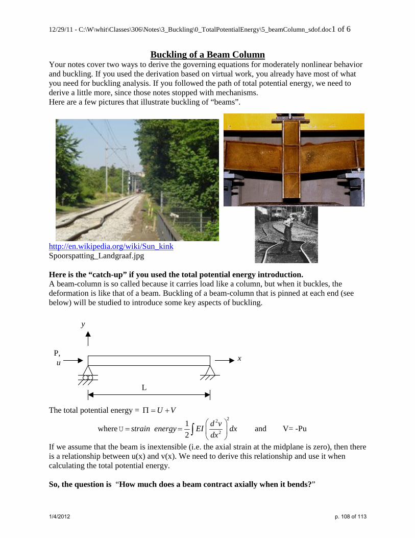
12/29/11 - C:\W\whit\Classes\306\Notes\3_Buckling\0_TotalPotentialEnergy\5_beamColumn_sdof.doc1 of 6
Buckling of a Beam Column Your notes cover two ways to derive the governing equations for moderately nonlinear behavior and buckling. If you used the derivation based on virtual work, you already have most of what you need for buckling analysis. If you followed the path of total potential energy, we need to derive a little more, since those notes stopped with mechanisms. Here are a few pictures that illustrate buckling of “beams”.
http://en.wikipedia.org/wiki/Sun_kink Spoorspatting_Landgraaf.jpg Here is the “catch-up” if you used the total potential energy introduction. A beam-column is so called because it carries load like a column, but when it buckles, the deformation is like that of a beam. Buckling of a beam-column that is pinned at each end (see below) will be studied to introduce some key aspects of buckling.
y
x
L
P, u
The total potential energy = U VΠ = +
where22
212
d vstrain energy EI dxdx
= =
∫U and V= -Pu
If we assume that the beam is inextensible (i.e. the axial strain at the midplane is zero), then there is a relationship between u(x) and v(x). We need to derive this relationship and use it when calculating the total potential energy. So, the question is “How much does a beam contract axially when it bends?”
1/4/2012 p. 108 of 113

12/29/11 - C:\W\whit\Classes\306\Notes\3_Buckling\0_TotalPotentialEnergy\5_beamColumn_sdof.doc2 of 6
This contraction cannot be ignored in stability analysis. We will assume that the midplane of the beam neither shortens nor lengthens. However, when the beam bends, its projection on the horizontal axis decreases. (i.e. it gets shorter... it will never get longer!) ... but how much shorter? The details of the derivation are given in a page or so in an Appendix. The derivation shows that
2 2
0
1 1 (for this problem)2 2
L dv dvu dx V P dxdx dx
= ⇒ = − ∫ ∫
This formula for “u” is actually the amount of shortening for any Euler-Bernoulli beam, regardless of the boundary conditions… so remember this formula! Now we have expressions for U and V in terms of v(x), so we can proceed to assume a kinematically admissible solution and obtain an approximate solution. Now we have the total potential energy for a beam that includes the first approximation of geometric nonlinearity, which is all we will consider. The result is
2 22
2
1 12 2
d v dvU V EI dx P dxdx dx
Π = + = −
∫ ∫
We must be careful about the sign of the second integral. Why? Hint: What if the load was applied at the right end? Approximate solution for the critical load
Assume: v ax
L= sin
π (satisfies all kinematic constraints)
Substitution into the formulas for strain energy and potential of an applied load yields 4 2 2 2
34 4a EI a PU and VL L
π π= = −
The only unknown is “a”, so the equilibrium equation is ∂Π∂
= = −FHG
IKJ
LNMM
OQPPa
L aL
EIL
P04
2 2
2
2
2π π
For this equation to be satisfied, either a = 0 (in which case P can be any value) or P EIL
=π2
2 .
Next we consider the stability of these equilibrium configurations. Recall that we examine the
sign of 2
2a∂ Π∂
to determine the stability. In particular, the structure is stable only if 2
2 0a
∂ Π>
∂.
∂
∂= −
FHG
IKJ
2
2
2 2
22Π
a LEI
LPπ π
1/4/2012 p. 109 of 113

12/29/11 - C:\W\whit\Classes\306\Notes\3_Buckling\0_TotalPotentialEnergy\5_beamColumn_sdof.doc3 of 6
Hence, the structure is stable only if 2
2
EIPL
π< . The critical load (also referred to as the
buckling load or Euler buckling load) is the load at which there is transition from stable to
unstable behavior. (i.e. when 2
2 0a
∂ Π=
∂) This load is
2
2
EIPL
π= .
This happens to be exact solution. Of course, normally we are not so lucky.
Matrix Form for Beams 2 22
2
22
2 2
2 22
2 2
1 12 2
If we assume v = Ni i
i i
i
j i i i
i j
d v dvU V EI dx P dxdx dxq
d N dNd v dvEI dx P dxq dx dx dx dx
d N d N dN dNEI dx P dxq q dx dx dx dx
Π = + = −
Σ
∂Π= −
∂
∂ Π= −
∂ ∂
∫ ∫
∫ ∫
∫ ∫
In this problem, when P is positive, there is a compressive axial force in the beam. This could get confusing. Let’s adopt the sign convention and definition that P is the axial force inside the beam and that tension is positive. In that case the equation becomes
2 22
2 2j i i i
i j
d N d N dN dNEI dx P dxq q dx dx dx dx∂ Π
= +∂ ∂ ∫ ∫
… and we will be careful to put the right value of “P” into the formula. We will not prove it here, but if the axial force varies with x, the P should be put inside the integral, as follows:
2 22
2 2j i i i
i j
d N d N dN dNEI dx P dxq q dx dx dx dx∂ Π
= +∂ ∂ ∫ ∫
This is the form that was obtained using Virtual Work.
1/4/2012 p. 110 of 113

12/29/11 - C:\W\whit\Classes\306\Notes\3_Buckling\0_TotalPotentialEnergy\5_beamColumn_sdof.doc4 of 6
Total Potential Energy and Virtual Work Once we derive the matrix form of the equations, the formulas based on Virtual Work and total potential energy are identical. The key is to recognize that the second derivative of the total potential energy is the coefficient matrix K in the equation 0Kq = and that the critical load corresponds to when this matrix becomes singular. It becomes singular when 0K = . For a one dof problem, this is just K=0. When there is more than one dof,
2 2
where the unknowns and the critical load occurs when 0ij ii j i j
K qq q q q∂ Π ∂ Π
= = =∂ ∂ ∂ ∂
. As
discussed earlier, for other than very small problems, finding the critical loads is accomplished by solving an eigenvalue problem of the form ( )0
10
K K q 0
K K q qThis is the standard form for eigenvalve problem if we take eigenvalues
σ
σ
λ
λλ
−
+ =
= −= −
Since Virtual Work also gives us the stiffness matrix (and it is identical), we do not need to distinguish whether the equations were obtained using total potential energy or Virtual Work. Disclaimer: The notes are in transition. The original notes were based on total potential energy, so some of the examples are not written in the general form yet.
1/4/2012 p. 111 of 113

12/29/11 - C:\W\whit\Classes\306\Notes\3_Buckling\0_TotalPotentialEnergy\5_beamColumn_sdof.doc5 of 6
Appendix: Shortening of Bent Beam Define: S ≡ coordinate along midplane of beam
Assume: Beam is inextensible ⇒ =z dS L0Left
Right
where dS= differential length along midplane of deformed beam. We will derive an expression for 0L in terms of v(x). Ultimately, it will give us the relationship between the projected length of the beam and the deformation. ( ) ( ) ( ) ( ) ( )
12
2 2 2 2 2
2
2
(Note that since y=0 before deformation)
Divide by (dx) and take the square root of both sides to obtain
1
dS dx dy dx dv y v
dS dvdx dx
= + = + =
= +
12
2 2
1 1
2
0 1x x
right end
left endx x
dS dvL dS dx dxdx dx
= = = +
∫ ∫ ∫
This is messy and we still do not have an expression for the projected length. Since the actual rotations are small, we can obtain a simple and accurate approximation for the square root term
using a Taylor series expansion. A first order Taylor series takes the form ( ) (0) dFF a F ada
= + .
In our case, 2dva
dx ≡
and ( ) ( )1/ 21F a a= + .The Taylor series is then
( ) ( )1/ 2
0
(0) 1 12a
d aF a F a ada =
= + + = +
Therefore
122 211 1
2dv dvdx dx
+ ≈ +
This approximation is much easier to work with. The expression for 0L is now
( )2 2 2 2
1 1 1 1
2 2 21
0 2 121 112 2
x x x x
x x x x
dv dv dvL dx dx dx dx x xdx dx dx
≈ + = + = + − ∫ ∫ ∫ ∫
Since the original projected length was L0 and the new length is 2 1x x− , the change in length is
∴ = − FHG
IKJz∆ Length 1
2
2
1
2 dydx
dxx
x
y,v
P
x
L0
Shortening
1/4/2012 p. 112 of 113

12/29/11 - C:\W\whit\Classes\306\Notes\3_Buckling\0_TotalPotentialEnergy\5_beamColumn_sdof.doc6 of 6
Note that we will approximate the integral limits as 0->L… since to do otherwise great complication. What is the relationship between Length ∆ and the end displacement of the beam? Comment
If we were to choose to define dvadx
≡
, we would have had to go to the next term in the Taylor
series expansion, because the linear term (the term involving the first derivative of F) would be zero… but the final result is the same.
Influence of boundary conditions on critical load
From Brush and Almroth
1/4/2012 p. 113 of 113