volume 209 no. 2 april 2003 journal of mathematics - msp
TRANSCRIPT

PACIFIC JOURNAL OF MATHEMATICS
Volume 209 No. 2 April 2003
PacificJournalofM
athematics
2003Vol.209,N
o.2
PacificJournal ofMathematics
Volume 209 No. 2 April 2003

PACIFIC JOURNAL OF MATHEMATICS
http://www.pjmath.org
Founded in 1951 by
E. F. Beckenbach (1906–1982) F. Wolf (1904–1989)
EDITORS
Vyjayanthi ChariDepartment of Mathematics
University of CaliforniaRiverside, CA 92521-0135
Robert FinnDepartment of Mathematics
Stanford UniversityStanford, CA [email protected]
Kefeng LiuDepartment of Mathematics
University of CaliforniaLos Angeles, CA 90095-1555
V. S. Varadarajan (Managing Editor)Department of Mathematics
University of CaliforniaLos Angeles, CA 90095-1555
Darren LongDepartment of Mathematics
University of CaliforniaSanta Barbara, CA 93106-3080
Jiang-Hua LuDepartment of Mathematics
The University of Hong KongPokfulam Rd., Hong Kong
Sorin PopaDepartment of Mathematics
University of CaliforniaLos Angeles, CA 90095-1555
Sorin PopaDepartment of Mathematics
University of CaliforniaLos Angeles, CA 90095-1555
Jie QingDepartment of Mathematics
University of CaliforniaSanta Cruz, CA 95064
Jonathan RogawskiDepartment of Mathematics
University of CaliforniaLos Angeles, CA 90095-1555
Paulo Ney de Souza, Production Manager Silvio Levy, Senior Production Editor Nicholas Jackson, Production Editor
SUPPORTING INSTITUTIONSACADEMIA SINICA, TAIPEI
CALIFORNIA INST. OF TECHNOLOGY
CHINESE UNIV. OF HONG KONG
INST. DE MATEMÁTICA PURA E APLICADA
KEIO UNIVERSITY
MATH. SCIENCES RESEARCH INSTITUTE
NEW MEXICO STATE UNIV.OREGON STATE UNIV.PEKING UNIVERSITY
STANFORD UNIVERSITY
UNIVERSIDAD DE LOS ANDES
UNIV. OF ARIZONA
UNIV. OF BRITISH COLUMBIA
UNIV. OF CALIFORNIA, BERKELEY
UNIV. OF CALIFORNIA, DAVIS
UNIV. OF CALIFORNIA, IRVINE
UNIV. OF CALIFORNIA, LOS ANGELES
UNIV. OF CALIFORNIA, RIVERSIDE
UNIV. OF CALIFORNIA, SAN DIEGO
UNIV. OF CALIF., SANTA BARBARA
UNIV. OF CALIF., SANTA CRUZ
UNIV. OF HAWAII
UNIV. OF MONTANA
UNIV. OF NEVADA, RENO
UNIV. OF OREGON
UNIV. OF SOUTHERN CALIFORNIA
UNIV. OF UTAH
UNIV. OF WASHINGTON
WASHINGTON STATE UNIVERSITY
These supporting institutions contribute to the cost of publication of this Journal, but they are not owners or publishers and have no respon-sibility for its contents or policies.
See inside back cover or www.pjmath.org for submission instructions.
Regular subscription rate for 2006: $425.00 a year (10 issues). Special rate: $212.50 a year to individual members of supporting institutions.Subscriptions, requests for back issues from the last three years and changes of subscribers address should be sent to Pacific Journal ofMathematics, P.O. Box 4163, Berkeley, CA 94704-0163, U.S.A. Prior back issues are obtainable from Periodicals Service Company, 11Main Street, Germantown, NY 12526-5635. The Pacific Journal of Mathematics is indexed by Mathematical Reviews, Zentralblatt MATH,PASCAL CNRS Index, Referativnyi Zhurnal, Current Mathematical Publications and the Science Citation Index.
The Pacific Journal of Mathematics (ISSN 0030-8730) at the University of California, c/o Department of Mathematics, 969 Evans Hall,Berkeley, CA 94720-3840 is published monthly except July and August. Periodical rate postage paid at Berkeley, CA 94704, and additionalmailing offices. POSTMASTER: send address changes to Pacific Journal of Mathematics, P.O. Box 4163, Berkeley, CA 94704-0163.
PUBLISHED BY PACIFIC JOURNAL OF MATHEMATICSat the University of California, Berkeley 94720-3840
A NON-PROFIT CORPORATIONTypeset in LATEX
Copyright ©2006 by Pacific Journal of Mathematics
PACIFIC JOURNAL OF MATHEMATICSVol. 209, No. 2, 2003
THE DISCRIMINANT OF A SYMPLECTIC INVOLUTION
Gregory Berhuy, Marina Monsurro, and Jean-Pierre Tignol
An invariant for symplectic involutions on central simplealgebras of degree divisible by 4 over fields of characteristicdifferent from 2 is defined on the basis of Rost’s cohomologicalinvariant of degree 3 for torsors under symplectic groups. Werelate this invariant to trace forms and show how its trivialityyields a decomposability criterion for algebras of degree 8 withsymplectic involution.
1. Introduction and statement of results.
In contrast with orthogonal involutions, for which invariants correspondingto the discriminant and Clifford algebras of quadratic forms are defined, no“classical” invariant is known for symplectic involutions on central simplealgebras, besides the signature (see [6, (11.10)]). Using the cohomologicalinvariant of degree 3 defined by Rost for torsors under simply connectedabsolutely simple linear algebraic groups, we introduce an invariant of sym-plectic involutions on central simple algebras of degree a multiple of 4 withvalues in the third Galois cohomology group of the center with coefficients±1 and give an alternative description in terms of trace forms. We callthis invariant the discriminant since it is the first nontrivial invariant, andbecause it is directly linked to the discriminant of Hermitian forms, see Ex-ample 2. Even though its definition is elementary, Rost’s computation ofthe invariants of torsors under symplectic groups is needed to prove thatthere is no other cohomological invariant of degree 3 and to establish therelationship with trace forms. In the final section, we prove that symplecticinvolutions with trivial discriminant on central simple algebras of degree 8and index 4 afford a special type of decomposition. In a sequel to this paper,the discriminant is used to give examples of non R-trivial adjoint symplecticgroups of even index.
1.1. Definition of the discriminant. Throughout this paper, F denotesa field of characteristic different from 2. Let A be a finite-dimensional centralsimple F -algebra, and θ : A → A be an anti-automorphism of order 2. Werecall that θ is called a symplectic involution on A if, after scalar extensionto a splitting field, θ is adjoint to an alternating form, see [6, (2.5)]. Fromnow on, we suppose the involution θ is of this type. In this case, the degreedegA is necessarily an even integer n = 2m.
201

202 GREGORY BERHUY, MARINA MONSURRO, AND JEAN-PIERRE TIGNOL
The symplectic group Sp(A, θ) is the group scheme over F defined by
Sp(A, θ)(E) = x ∈ A⊗F E | θ(x)x = 1for any commutative F -algebra E.
Let Sym(A, θ) be the F -vector space of elements in A fixed by θ,
Sym(A, θ) = x ∈ A | θ(x) = x.We denote by Sym(A, θ)× the set of units in Sym(A, θ),
Sym(A, θ)× = Sym(A, θ) ∩A×.We recall that the pfaffian reduced norm is the homogeneous polynomial
function of degree m
Nrpθ : Sym(A, θ) → F
uniquely determined by the following conditions:
Nrpθ(1) = 1 and Nrpθ(x)2 = NrdA(x) for x ∈ Sym(A, θ),
see [6, p. 19].The cohomology set H1
(F,Sp(A, θ)
)can be represented as
H1(F,Sp(A, θ)
)' Sym(A, θ)×/∼(1)
where ∼ is the equivalence relation defined by x ∼ y if and only if thereexists u ∈ A× such that y = uxθ(u), see [6, (29.24)].
Let Gm be the multiplicative group. The Kummer exact sequence
1 → µ2 → Gm2−→Gm → 1
allows us to identify the cohomology sets H1(F, µ2) and H2(F, µ2) respec-tively with the quotient F×/F×2 and with the 2-torsion subgroup of theBrauer group. For all x ∈ F×, we denote by (x)2 ∈ H1(F, µ2) the cohomol-ogy class associated to xF×2. Similarly, we denote by [A] ∈ H2(F, µ2) thecohomology class associated to the Brauer class of A. We define
∆θ : Sym(A, θ)× → H3(F, µ2)
as the map given by the cup-product
∆θ(s) =(Nrpθ(s)
)2∪ [A].
It follows from the properties of Nrpθ (see the proof of Proposition 1below) that ∆θ is well-defined on the set of equivalence classes under therelation ∼. The induced map on the quotient can be interpreted under thebijection (1) as the Rost invariant of H1
(F,Sp(A, θ)
), see [6, p. 440].
Since Nrpθ is homogeneous of degree m, we obtain, for α ∈ F× ands ∈ Sym(A, θ)×, the following relation:
∆θ(αs) =(αm Nrpθ(s)
)2∪ [A] =
∆θ(s) if m is even,∆θ(s) + (α)2 ∪ [A] if m is odd.
(2)
THE DISCRIMINANT OF A SYMPLECTIC INVOLUTION 203
Therefore, if m is even one can define a relative invariant for symplecticinvolutions on A as follows:
Definition. Let A be a central simple algebra over F of degree n = 2m ≡0 mod 4. Let θ and σ be symplectic involutions on A. There exists (see [6,(2.7)]) s ∈ Sym(A, θ)× such that
σ = Int(s) θwhere Int(s) denotes the inner automorphism associated with s,
Int(s)(x) = sxs−1 for x ∈ A.The element s is uniquely determined up to multiplication by an element ofF×. By (2), it follows that ∆θ(s) ∈ H3(F, µ2) only depends on σ, since mis even. We call this element the discriminant of σ with respect to θ anddenote it by ∆θ(σ). Thus,
∆θ(σ) =(Nrpθ(s)
)2∪ [A] ∈ H3(F, µ2).
In the case m = 2, an analogue of this invariant has been studied in [6,§16.B], where it is denoted by jθ(σ). Theorem (16.19) of [6] shows that thisinvariant classifies, up to conjugation, symplectic involutions on a centralsimple algebra of degree 4.
In Section 2 we establish the following elementary result:
Proposition 1.(a) The discriminant ∆θ(σ) only depends on the conjugacy classes of θ
and σ, namely, if u, v ∈ A× and
θ′ = Int(u) θ Int(u)−1, σ′ = Int(v) σ Int(v)−1,
then
∆θ′(σ′) = ∆θ(σ).
In particular, if σ and θ are conjugate, then ∆θ(σ) = 0.(b) Let ρ, σ and θ be symplectic involutions on A; then
∆ρ(σ) = ∆ρ(θ) + ∆θ(σ) and ∆θ(σ) = ∆σ(θ).
If the Schur index indA divides 12 degA, i.e., if A 'M2(A0) for some cen-
tral simple F -algebra A0, then A carries hyperbolic symplectic involutions,such as γ ⊗ θ0, where γ is the (unique) symplectic involution on M2(F )and θ0 is an arbitrary orthogonal involution on A0. Since all hyperbolicinvolutions are pairwise conjugate, we may set ∆ = ∆θ for any hyperbolicsymplectic involution θ.
Example 2. Consider the algebra A = EndQ V , where Q is a quaterniondivision F -algebra and V is an m-dimensional Q-vector space. Symplecticinvolutions on A are then adjoint to Hermitian forms on V with respect to
204 GREGORY BERHUY, MARINA MONSURRO, AND JEAN-PIERRE TIGNOL
the conjugation involution on Q. Suppose that m is even and let σ be theinvolution adjoint to a fixed Hermitian form h on V . Let
h = 〈α1, . . . , αm〉
be the diagonalization of h relative to some orthogonal basis e of V (α1, . . . ,αm ∈ F×), then
∆(σ) =((−1)m/2α1 . . . αm
)2∪ [Q].
Indeed, let θ be the hyperbolic involution adjoint to the Hermitian form withdiagonalization 〈1,−1, . . . , 1,−1〉 relative to the basis e. Then, identifyingA with Mm(Q) by e, we get
σ = Int diag(α1,−α2, . . . , αm−1,−αm) θ,
and we can compute ∆(σ) = ∆θ(σ) by Lemma 9(e) below.
Note that if V0 ⊂ V is the F -subspace spanned by e, then A = (EndF V0)⊗Q, and we obtain a decomposition σ = σ0 ⊗ γ where σ0 is the involutionadjoint to the bilinear form on V0 with diagonalization 〈α1, . . . , αm〉 relativeto e, and γ is the canonical (conjugation) involution on Q.
This example can be slightly generalized:
Example 3. Consider the algebra A = A0 ⊗F Q where Q is a quaternionF -algebra and A0 is a central simple F -algebra. Let σ0 be an orthogonalinvolution on A0, γ the canonical involution on Q, and
σ = σ0 ⊗ γ.
Suppose that indA0 divides 12 degA0. Then
∆(σ) = (discσ0)2 ∪ [Q],(3)
where discσ0 ∈ F×/F×2 is the discriminant of the orthogonal involutionσ0 (see [6, §7]). Indeed, let θ0 be a hyperbolic orthogonal involution on A0
and let x0 ∈ Sym(A0, θ0)× be such that σ0 = Int(x0) θ0. The involutionθ = θ0 ⊗ γ is hyperbolic, and we have σ = Int(x0 ⊗ 1) θ, so that
∆(σ) =(Nrpθ(x0 ⊗ 1)
)2∪ [A].
Now, by Lemma 9(d), Nrpθ(x0 ⊗ 1) = NrdA0(x0). Equation (3) follows,since discσ0 is represented by NrdA0(x0), and
(NrdA0(x0)
)2∪ [A0] = 0.
1.2. Trace forms. Let A be an arbitrary central simple F -algebra. Forevery involution σ : A→ A, the associated trace form Tσ : A→ F is definedas follows:
Tσ(x) = TrdA(σ(x)x
)

THE DISCRIMINANT OF A SYMPLECTIC INVOLUTION 205
where TrdA denotes the reduced trace. Denote by T+σ the restriction of Tσ
to Sym(A, σ); this form can also be seen as the restriction to Sym(A, σ) ofthe form TA : A→ F defined by
TA(x) = TrdA(x2).
As is the case with involutions of the other types (see [6, §11]), the dis-criminant of symplectic involutions can be expressed in terms of trace forms;indeed we have the following result:
Theorem 4. Let A be a central simple algebra over F and let θ and σ besymplectic involutions on A. The class in the Witt ring WF of the differenceT+σ − T+
θ lies in the third power of the fundamental ideal, namely
T+σ − T+
θ ∈ I3F.
Moreover, if e3 : I3F → H3(F, µ2) denotes the Arason invariant, we obtain
e3(T+σ − T+
θ ) =
∆θ(σ) if degA ≡ 0 mod 4,0 if degA ≡ 2 mod 4.
A proof of this result is given in Section 3 below. For the trace forms Tσ,we have the following result:
Corollary 5. Keeping the notation of the previous theorem, we have Tσ −Tθ ∈ I4F and
e4(Tσ − Tθ) =
(−1)2 ∪∆θ(σ) if degA ≡ 0 mod 4,0 if degA ≡ 2 mod 4,
where e4 : I4F → H4(F, µ2) denotes the degree 4 invariant.
Proof. Let T−σ be the restriction of Tσ (or of −TA) to the space of skew-symmetric elements in A. We have
Tσ = T+σ + T−σ and TA = T+
σ − T−σ ,
so that Tσ = 2T+σ − TA. Similarly, Tθ = 2T+
θ − TA, so that
Tσ − Tθ = 2(T+σ − T+
θ ),
hence the corollary is a direct consequence of the previous theorem.
In the special case where θ is hyperbolic we get:
Proposition 6. Suppose A = M2(A0) for some central simple F -algebraA0, and let θ be a hyperbolic symplectic involution on A. Then T+
θ is Witt-equivalent to 〈2〉 · TA0, and Tθ is hyperbolic. If degA ≡ 2 mod 4, then Ais split, hence every symplectic involution on A is hyperbolic. If degA ≡0 mod 4, then, for any symplectic involution σ on A, we have Tσ ∈ I4F and
e4(Tσ) = (−1)2 ∪∆(σ).
The proof is at the end of Section 3.

206 GREGORY BERHUY, MARINA MONSURRO, AND JEAN-PIERRE TIGNOL
1.3. Decomposability of symplectic involutions. Section 4 below willbe devoted to the relations between the discriminant and the decompos-ability of symplectic involutions as tensor products of involutions definedon subalgebras. Our main result is concerned with degree 8 algebras withindex dividing 4. Such algebras can be written in the form A = M2(A0),where A0 is a central simple algebra of degree 4, hence they carry hyperbolicsymplectic involutions. The case indA = 1 is trivial, since every symplecticinvolution on a split algebra is hyperbolic, and is omitted in the followingtheorem:
Theorem 7. Let A be a central simple F -algebra of degree 8 having index2 or 4. For any symplectic involution σ on A, there is a decomposition
(A, σ) = (Q, γ)⊗F (A0, σ0)
where Q is a quaternion subalgebra, A0 is its centralizer (which is a centralsimple F -subalgebra of degree 4 in A), γ is the conjugation involution on Qand σ0 is an orthogonal involution on A0.
When indA = 2, this theorem is easily proved and can be readily general-ized to any degree, see Example 2 or [1, Proposition 3.4]. The case indA = 4is treated in Section 4.
Theorem 7 shows that the discriminant of a symplectic involution σ on acentral simple F -algebra of degree 8 and index 2 or 4 can be computed asin Example 3 above. The following theorem gives a necessary and sufficientcondition for the discriminant to be trivial.
Theorem 8. Let A be a central simple F -algebra of degree 8 with indexdividing 4. For any symplectic involution σ on A, ∆(σ) = 0 if and onlythere is a decomposition
(A, σ) = (A1, σ1)⊗F (A2, σ2)⊗F (A3, γ3)
where A1, A2, A3 are quaternion subalgebras of A, σ1, σ2 are orthogonalinvolutions on A1 and A2 respectively, γ3 is the conjugation involution onA3, and A1 is split,
A1 'M2(F ).
A proof is given in Section 4.
2. Discriminants and Pfaffian norms.
The goal of this section is to prove Proposition 1. Throughout the section,A denotes a central simple F -algebra of degree n = 2m.
Lemma 9. Let σ and θ be symplectic involutions on A and let s be anelement in Sym(A, θ)× such that σ = Int(s) θ. Then:
THE DISCRIMINANT OF A SYMPLECTIC INVOLUTION 207
(a) For every x ∈ Sym(A, σ) ∩ Sym(A, θ),
Nrpσ(x) = Nrpθ(x).
(b) For every x ∈ Sym(A, θ), the product sx lies in Sym(A, σ) and
Nrpσ(sx) = Nrpθ(s) Nrpθ(x).
(c) For every x ∈ Sym(A, θ)×,
Nrpθ(x−1) = Nrpθ(x)
−1.
(d) Suppose A = A1⊗F A2 for some central simple F -algebras A1, A2 ⊂ Aof degree n1 = 2m1 and n2 = 2m2 respectively; if x1 ∈ A1 and x2 ∈ A2
are such that x1 ⊗ x2 ∈ Sym(A, θ), then
Nrpθ(x1 ⊗ x2) = NrdA1(x1)m2 NrdA2(x2)m1 .
(e) Suppose A = Mr(A0) and θ((aij)1≤i,j≤r
)=(θ0(aij)
)t1≤i,j≤r for some
symplectic involution θ0 on the central simple F -algebra A0. For thediagonal matrix x = diag(x1, . . . , xr) with xi ∈ Sym(A0, θ0) for i =1, . . . , r, we have
Nrpθ(x) = Nrpθ0(x1) . . .Nrpθ0(xr).
Proof. (a) Let t be an indeterminate over F . Define
Prpσ,x(t) = Nrpσ(t− x) ∈ F [t], Prpθ,x(t) = Nrpθ(t− x) ∈ F [t].
Those polynomials, called pfaffian characteristic polynomials in [6, p. 19],are monic and satisfy
Prp2σ,x = PcrdA,x = Prp2
θ,x,
where PcrdA,x(t) = NrdA(t)(t − x) is the reduced characteristic polynomialof x. Therefore, Prpσ,x(t) = Prpθ,x(t), and evaluation at t = 0 yieldsNrpσ(x) = Nrpθ(x).
(b) Straightforward calculations show that σ(sx) = sx if θ(x) = x. Letus consider the two sides of the equality we aim to prove as polynomialfunctions of x. The squares of the two sides are equal since the reducednorm is multiplicative, hence they are equal up to sign. Moreover, they areequal and nonzero for x = 1 in view of Part (a). Hence, they are equal forall x.
(c) We apply (b) with x = s−1 and use the relation Nrpσ(1) = 1.(d) By taking the square root on both sides of the equation
PcrdA,x1⊗x2 = (PcrdA1,x1)n2(PcrdA2,x2)
n1 ,
we obtain
Prpθ,x1⊗x2= (PcrdA1,x1)
m2(PcrdA2,x2)m1 .
The property follows by considering the constant terms.

208 GREGORY BERHUY, MARINA MONSURRO, AND JEAN-PIERRE TIGNOL
(e) As in the preceding case, the property follows by extracting the monicsquare root of each side of the equation
PcrdA,x = PcrdA0,x1 . . .PcrdA0,xr .
Proposition 1 easily follows from the lemma above. Indeed, if σ = Int(s)θ, so that ∆θ(σ) =
(Nrpθ(s)
)2∪ [A], then θ = Int(s−1) σ and hence
∆σ(θ) =(Nrpσ(s−1)
)2∪ [A]. Now Lemma 9 shows that
Nrpσ(s−1) = Nrpθ(s)
−1,
hence(Nrpσ(s−1)
)2
=(Nrpθ(s)
)2, and so ∆σ(θ) = ∆θ(σ). If ρ is another
symplectic involution, and if t ∈ Sym(A, ρ) is such that θ = Int(t) ρ, thenσ = Int(st) ρ. Part (b) of Lemma 9 yields
Nrpσ(st) = Nrpθ(s) Nrpθ(t).
Moreover, Part (a) shows that Nrpσ(st) = Nrpρ(st) and Nrpθ(t) = Nrpρ(t).Therefore, the preceding equality can be written as
Nrpρ(st) = Nrpθ(s) Nrpρ(t).
It follows that
∆ρ(σ) =(Nrpρ(st)
)2∪ [A]
=(Nrpθ(s)
)2∪ [A] +
(Nrpρ(t)
)2∪ [A] = ∆θ(σ) + ∆ρ(θ),
which completes the proof of Part (b) of Proposition 1.Now let v ∈ A× and σ′ = Int(v)σInt(v)−1, so that σ′ = Int
(vsθ(v)
)θ.
Then,
∆θ(σ′) =(Nrpθ(vsθ(v))
)2∪ [A].
By [6, (2.13)], Nrpθ(vsθ(v)
)= NrdA(v) Nrpθ(s). Since
(NrdA(v)
)2∪ [A] = 0,
it follows that
∆θ(σ′) = ∆θ(σ).
Similarly, if θ′ is a symplectic involution conjugate to θ, then ∆σ′(θ′) =∆σ′(θ). Now, Part (b) of Proposition 9 shows that ∆θ′(σ′) = ∆σ′(θ′) and∆θ(σ′) = ∆σ′(θ). Therefore,
∆θ′(σ′) = ∆θ(σ′).
We already observed that ∆θ(σ′) = ∆θ(σ), hence
∆θ′(σ′) = ∆θ(σ)
and the proof of Proposition 1 is complete.
THE DISCRIMINANT OF A SYMPLECTIC INVOLUTION 209
3. Discriminant and trace form.
In this section we prove Theorem 4 and Proposition 6.Let FieldsF be the category of fields containing F and let G be any alge-
braic group over F . We consider the functor
H1(G) : FieldsF → Sets*
where Sets* denotes the category of pointed sets, associating to every L ∈FieldsF the Galois cohomology set H1(L,G).
For any integer d ≥ 0, we let Q/Z(d − 1) = lim−→µ⊗(d−1)n , where µn is
the group of n-th roots of unity in a separable closure of F . We may thenconsider the functor
Hd(Q/Z(d− 1)
): FieldsF → Sets*
which carries L ∈ FieldsF to the Galois cohomology groupHd(L,Q/Z(d−1)
)(and forgets the group structure). The natural transformations H1(G) →Hd(Q/Z(d − 1)
)are called cohomological invariants of dimension (or de-
gree) d in [6, §31.B]. Since Hd(L,Q/Z(d − 1)
)is a group for L ∈ FieldsF ,
these invariants form a group. In reference to Rost’s “cohomological cy-cle module” M =
⊕d≥0H
d(•,Q/Z(d − 1)
)(see [8]), we denote it simply
by Invd(H1(G),M). (This group is denoted by Invd(G,Q/Z(d − 1)
)in [6,
§31.B].)Now let A be a central simple F -algebra of degree n = 2m and let θ
be a symplectic involution on A. We take for G the group GSp(A, θ) ofsymplectic similitudes; this is the algebraic group scheme defined by
GSp(A, θ)(E) = g ∈ A⊗F E | θ(g)g ∈ E×for any commutative F -algebra E. The set H1
(L,GSp(A, θ)
)is in one-
to-one correspondence with the set of conjugacy classes of symplectic in-volutions defined on AL = A ⊗F L, the class of θ being the distinguishedone (see [6, (29.23)]). The following proposition shows that for symplecticinvolutions there is no (nontrivial) cohomological invariant of degree 1 or 2.
Proposition 10. If the algebra A is split, we have H1(L,GSp(A, θ)
)= 1
for every L ∈ FieldsF , so that
Invd(H1(GSp(A, θ)
),M)
= 0 for all d.
If A is not split, we have
Invd(H1(GSp(A, θ)
),M)
= 0 for d = 1, 2
and
Inv3(H1(GSp(A, θ)
),M)
=
0 if degA ≡ 2 mod 4,Z/2Z if degA ≡ 0 mod 4.

210 GREGORY BERHUY, MARINA MONSURRO, AND JEAN-PIERRE TIGNOL
Proof. Every symplectic involution on a split algebra is hyperbolic. There-fore, when A is split, H1
(L,GSp(A, θ)
)= 1 for all L ∈ FieldsF .
For the rest of the proof, we may thus assume that A is not split. Let
µ : GSp(A, θ) → Gm
be the homomorphism which associates to each similitude g its multiplierµ(g) = θ(g)g. The cohomology sequence induced by the exact sequence
1 → Sp(A, θ) → GSp(A, θ)µ−→ Gm → 1
yields for every L ∈ FieldsF the exact sequence
L× → H1(L,Sp(A, θ)
)→ H1
(L,GSp(A, θ)
)→ 1
since H1(L,Gm) = 1 by Hilbert’s Theorem 90. Therefore, for every d, wehave an exact sequence
0 → Invd(H1(GSp(A, θ)
),M)→ Invd
(H1(Sp(A, θ)
),M)→ Invd(Gm,M).
For d = 1 or 2, we obtain, by [6, (31.15)], Invd(H1(Sp(A, θ)
),M)
= 0 andhence
Invd(H1(GSp(A, θ)
),M)
= 0.
The group Inv3(H1(Sp(A, θ)
),M)
is of order 2, the nontrivial element beingthe Rost invariant ∆θ defined in the introduction. Equation (2) shows thatthis invariant is zero in Inv3(Gm,M) if and only if degA ≡ 2 mod 4.
When degA ≡ 0 mod 4, the unique nontrivial invariant of degree 3 is thediscriminant. Our next goal is to give an explicit description of this invariantin terms of trace forms.
Let T+θ : Sym(A, θ) → F be the quadratic form
T+θ (x) = TrdA(θ(x)x) = TrdA(x2).
This forms only depends, up to isometry, on the conjugacy class of θ since,if θ′ = Int(v) θ Int(v)−1 for some v ∈ A×, then Int(v) defines an isom-etry between T+
θ and T+θ′ . Consider L ∈ FieldsF . The map sending every
symplectic involution σ : AL → AL to the discriminant
disc(T+σ − T+
θ ) ∈ L×/L×2 = H1(L, µ2)
defines a cohomological invariant H1(GSp(A, θ)
)→ H1(µ2). By Proposi-
tion 10, this invariant is trivial, hence T+σ − T+
θ ∈ I2L. Similarly, the mapsending every symplectic involution σ to the Witt (-Clifford) invariant
e2(T+σ − T+
θ ) ∈ H2(L, µ2)
defines a cohomological invariant of degree 2. Again, by Proposition 10,we get e2(T+
σ − T+θ ) = 0, and hence T+
σ − T+θ ∈ I3L using Merkurjev’s
theorem. This proves the first part of Theorem 4. Note that the equality
THE DISCRIMINANT OF A SYMPLECTIC INVOLUTION 211
e2(T+σ − T+
θ ) = 0 can also be derived from Queguiner’s explicit calculationof the Hasse invariant of trace forms in [7, p. 307].
Consider the map associating to every symplectic involution σ : AL → ALthe Arason invariant
e3(T+σ − T+
θ ) ∈ H3(L, µ2).
Using Proposition 10, we see that this invariant is trivial if degA ≡ 2 mod 4or if A is split. We claim that it coincides with the discriminant ∆θ(σ)if A is nonsplit and degA ≡ 0 mod 4. To prove this, it suffices to showthat it is nontrivial because, by Proposition 10, there is a unique nontrivialinvariant in Inv3
(H1(GSp(A, θ)
),M). Therefore, our goal is to find a field
L ∈ FieldsF and two symplectic involutions σ1, σ2 on AL such that e3(T+σ1−
T+σ2
) 6= 0. If θ is any involution on A, the equality
e3(T+σ1− T+
θ ) = e3(T+σ1− T+
σ2) + e3(T+
σ2− T+
θ )
shows that at least one of the terms e3(T+σ1−T+
θ ) and e3(T+σ2−T+
θ ) is nonzero,hence the invariant σ 7→ e3(T+
σ − T+θ ) is nontrivial.
After scalar extension to the function field of a suitable generalized Severi-Brauer variety (see [2]), we may assume that indA = 2 i.e., that A is Brauer-equivalent to a quaternion division algebra Q over F . Then, denoting by Van F -vector space of dimension m, we obtain
A ' Q⊗F EndF V.
For the rest of this section, we fix an isomorphism identifying A withQ ⊗ EndF V . Let b be a symmetric nondegenerate bilinear form on V .The symmetric square S2V and the exterior square
∧2 V are endowed withsymmetric bilinear forms bS
2and b∧2 respectively, defined by
bS2(x1 · x2, y1 · y2) = b(x1, y1)b(x2, y2) + b(x1, y2)b(x2, y1)
and
b∧2(x1 ∧ x2, y1 ∧ y2) = b(x1, y1)b(x2, y2)− b(x1, y2)b(x2, y1).
Lemma 11. Let Q = (α, β)F . On A = Q ⊗F EndF V , consider the sym-plectic involution σ = γ ⊗ adb, where γ is the quaternion conjugation on Qand adb is the (orthogonal ) involution adjoint to b. Then, the bilinear formB+σ (x, y) = TrdA(xy) on Sym(A, σ) (which is the polar form of the quadratic
form T+σ ) decomposes as an orthogonal sum
B+σ = bS
2 ⊥ 〈−α,−β, αβ〉 · b∧2.
Proof. Let Skew(EndF V, adb) be the F -vector space of endomorphisms f ofV such that adb(f) = −f , and let Q0 be the F -vector space of pure quater-nions in Q. A straightforward calculation shows that the decomposition
Sym(A, σ) =(F ⊗ Sym(EndF V, adb)
)⊕(Q0 ⊗ Skew(EndF V, adb)
)

212 GREGORY BERHUY, MARINA MONSURRO, AND JEAN-PIERRE TIGNOL
is orthogonal with respect to the form B+σ . Let B+
b and B−b be the restric-tions of the bilinear trace form B(f, g) = tr(fg) to Sym(EndF V, adb) andSkew(EndF V, adb) respectively. The decomposition above yields
B+σ = 〈2〉 ·B+
b ⊥ 〈2α, 2β,−2αβ〉 ·B−b .
The lemma follows, since, by [6, (11.4)] B+b ' 1
2bS2
and B−b ' −12b∧2.
If b = 〈a1, . . . , am〉 is a diagonalization of b, it is easily verified that
bS2 ' m〈2〉 ⊥
(⊥i<j 〈aiaj〉
)and b∧2 ' ⊥i<j 〈aiaj〉
(cf [6, p. 135]). The formula of the preceding lemma can then be written as
B+σ ' m〈2〉 ⊥ 〈1,−α,−β, αβ〉 · b∧2,
hence, in terms of quadratic forms,
T+σ = m〈2〉+ nQ · q∧2
where nQ denotes the norm form of Q and q∧2 is the quadratic form definedby q∧2(x) := b∧2(x, x).
Let b1 and b2 be two nonsingular symmetric bilinear forms on V , and let
σ1 = γ ⊗ adb1 , σ2 = γ ⊗ adb2be the symplectic involutions on A = Q ⊗ EndF V constructed as in thepreceding lemma. Observe that T+
σ1− T+
σ2= nQ · (q∧2
1 − q∧22 ), hence
e3(T+σ1− T+
σ2) = [Q] ∪ disc(q∧2
1 − q∧22 ).(4)
Explicit calculation shows that
disc(q∧21 − q∧2
2 ) = det b∧21 · det b∧2
2 = (det b1 · det b2)m−1.(5)
Adjoining an indeterminate to F if necessary, we may assume that there ex-ists an element t ∈ F× not belonging to Nrd(Q). By a theorem of Merkurjev,this element satisfies [Q] ∪ (t)2 6= 0. It is easy to find two bilinear forms b1and b2 on V such that det b1 ·det b2 = tF×2. Since m is even, it follows from(4) and (5) that the corresponding involutions σ1 and σ2 satisfy
e3(T+σ1− T+
σ2) 6= 0.
This completes the proof of Theorem 4.
We now turn to Proposition 6 and assume A = M2(F ) ⊗F A0. Since allhyperbolic involutions are conjugate, we may assume moreover θ = γ ⊗ θ0for some orthogonal involution θ0 on A0, where γ is the unique symplecticinvolution on M2(F ) (which is hyperbolic). As in Lemma 11, we have anorthogonal decomposition
Sym(A, θ) =(F ⊗ Sym(A0, θ0)
)⊕(Skew(M2(F ), γ)⊗ Skew(A0, θ0)
)which yields
T+σ = 〈2〉 · T+
θ0⊥ 〈2,−2,−2〉 · T−θ0 .

THE DISCRIMINANT OF A SYMPLECTIC INVOLUTION 213
Therefore, T+σ is Witt-equivalent to 〈2〉 · (T+
θ0− T−θ0) = 〈2〉 · TA0 . Since the
adjoint involution to Tθ is θ⊗θ, by [6, (11.1)], it is clear that Tθ is hyperbolicwhen θ is hyperbolic. If degA ≡ 2 mod 4, then degA0 is odd, hence A0 issplit. Therefore, A is also split. The other statements in Proposition 6follow from Corollary 5.
4. Discriminant and decomposability of involutions.
Our first goal in this section is to give a proof of Theorem 7. As observedin Section 1.3, the theorem is easy if indA = 2. Therefore, we assumeindA = 4. We may then represent A as
A = EndD V
where D is a division algebra of degree 4 and V is a 2-dimensional D-vectorspace. Let θ0 be an arbitrary symplectic involution on D. The involutionσ is adjoint to a Hermitian form h on V (with respect to θ0). Using anorthogonal basis of V relative to h, we may identify
A = M2(D) and σ = Int diag(u1, u2) θ0for some u1, u2 ∈ Sym(D, θ0)×, where
θ0((aij)1≤i,j≤2
)=(θ0(aij)
)t1≤i,j≤2
,
i.e., θ0 = t ⊗ θ on A = M2(F ) ⊗F D. Substituting Int(u1) θ0 for θ0, wemay assume u1 = 1. By [6, (16.16)], we may find a decomposition of D intoa tensor product of quaternion subalgebras stable under θ0,
D = Q1 ⊗F Q, θ0 = θ1 ⊗ γ
where θ1 is an orthogonal involution on Q1 and γ is the canonical involutionon Q. Moreover, we may assume u2 ∈ Q1. Then
σ = Int diag(1, u2) (t⊗ θ1 ⊗ γ) = σ0 ⊗ γ
with σ0 = Int diag(1, u2) t ⊗ θ1 on M2(F ) ⊗ Q1. Theorem 7 is thusproved. Note that the quaternion algebra Q is not uniquely determinedby [6, (16.16)].
Let us now prove Theorem 8, starting with the following general remark:
Lemma 12. For i = 1, 2, let Ai be a central simple F -algebra with involu-tions σi, θi. Assume:
(a) degA1 ≡ 2 mod 4 and σ1, θ1 orthogonal, and(b) degA2 ≡ 0 mod 4 and σ2, θ2 symplectic.
Then ∆θ1⊗θ2(σ1 ⊗ σ2) = 0.
Proof. Consider u1 ∈ Sym(A1, θ1)× and u2 ∈ Sym(A2, θ2)× such that
σ1 = Int(u1) θ1 and σ2 = Int(u2) θ2,

214 GREGORY BERHUY, MARINA MONSURRO, AND JEAN-PIERRE TIGNOL
hence
σ1 ⊗ σ2 = Int(u1 ⊗ u2) (θ1 ⊗ θ2).
Then ∆θ1⊗θ2(σ1⊗ σ2) =(Nrpθ1⊗θ2(u1⊗ u2)
)2∪ [A1⊗A2], and Lemma 9(d)
yields
Nrpθ1⊗θ2(u1 ⊗ u2) = NrdA1(u1)12
degA2 NrdA2(u2)12
degA1 .(6)
Since degA2 ≡ 0 mod 4, the first factor is a square. Moreover, since σ2 andθ2 are of symplectic type,
NrdA2(u2) = Nrpθ2(u2)2.
Therefore, Equation (6) shows that Nrpθ1⊗θ2(u1 ⊗ u2) ∈ F×2, so that
∆θ1⊗θ2(σ1 ⊗ σ2) = 0.
Even in the case degA = 8, there may be symplectic involutions θ, σ on Awhich do not decompose as in Lemma 12, even though ∆θ(σ) = 0. Indeed,there are examples of algebras with involution which do not contain anyinvariant quaternion subalgebra on which the restriction of the involutionis of orthogonal type. Suppose θ is a symplectic involution on a centralsimple algebra A of degree 8, and A1 ⊂ A is a quaternion subalgebra onwhich θ restricts to an orthogonal involution θ1. The restriction of θ to thecentralizer of A1 is then symplectic, hence [6, (16.16)] yields a decomposition
(A, θ) = (A1, θ1)⊗ (A2, θ2)⊗ (A3, γ3),
where A1, A2 and A3 are quaternion algebras, θ1 and θ2 are orthogonalinvolutions on A1 and A2 respectively, and γ3 is the canonical involutionon A3. This implies, in particular, that the signature of θ with respect toevery ordering of the field F is either 0 or 8. For example, if F = R is thefield of real numbers and θ is the involution adjoint to the Hermitian form〈1, 1, 1,−1〉 on the usual quaternion algebra H, then sgn θ = 4, and so A =M4(H) has no quaternion subalgebras on which θ restricts to an orthogonalinvolution. Therefore, even though ∆θ(θ) = 0, there is no decomposition asin Lemma 12. (See Example 13 for a subtler example.)
Returning to the proof of Theorem 8, we suppose until the end of thissection that A is a central simple F -algebra of degree 8, with index dividing4. Let σ be a symplectic involution on A, and suppose A1 ' M2(F ) is aninvariant subalgebra on which the restriction of σ is an orthogonal involution.In this situation, we have a decomposition A = A1 ⊗A′1, where A′1 denotesthe centralizer of A1, and σ = σ1 ⊗ σ′1, where σ1 and σ′1 are the restrictionsof σ to A1 and A′1 respectively. As A1 ' M2(F ), we can find a hyperbolicorthogonal involution θ1 on A1 and set
θ = θ1 ⊗ σ′1.

THE DISCRIMINANT OF A SYMPLECTIC INVOLUTION 215
The involution θ is hyperbolic of symplectic type and, by Lemma 12, wehave
∆(σ) = ∆θ(σ) = 0.
Conversely, let σ be a symplectic involution on A such that ∆(σ) = 0.To prove that σ leaves invariant a subalgebra of A isomorphic to M2(F ) onwhich it restricts to an orthogonal involution, we consider separately variouscases, depending on the index of A. If A is split, every symplectic involutionis hyperbolic and the property is a consequence of [1, Theorem 2.2]. IfindA = 2, we can always represent A in the form
A = EndQ V
where Q is a quaternion algebra and V is a 4-dimensional vector space overQ. The involution σ is then adjoint to a Hermitian form h on V (withrespect to the canonical involution γ on Q). Let e be an orthogonal basisfor h. Since h is determined by σ up to a factor in F×, we may assume thatthe diagonalization of h with respect to the basis e is 〈1, α1, α2, α3〉 withα1, α2, α3 ∈ F×. Let V0 ⊂ V be the F -subspace with basis e. We haveV = V0 ⊗F Q and
A = (EndF V0)⊗F Q, σ = σ0 ⊗ γ
where σ0 is the orthogonal involution on EndF V0 adjoint to the bilinearsymmetric form 〈1, α1, α2, α3〉. As in Example 2, ∆(σ) = (α1α2α3)2 ∪ [Q].Therefore, the condition ∆(σ) = 0 implies, by a theorem of Merkurjev, thatα1α2α3 ∈ NrdQ(Q×). Changing basis if necessary, we may assume thatα3 = α1α2. Then
〈1, α1, α2, α3〉 = 〈1, α1〉 ⊗ 〈1, α2〉.
This implies σ0 = σ1⊗σ2 on EndF V0 'M2(F )⊗M2(F ), where σ1 and σ2 arethe involutions adjoint to the bilinear forms 〈1, α1〉 and 〈1, α2〉, respectively.This proves the theorem in this case.
Finally, suppose indA = 4. As in the proof of Theorem 7 given at thebeginning of this section, we may then represent A as A = EndD V where Dis a division algebra of degree 4 and V is a 2-dimensionalD-vector space. Forthe rest of the proof, we use the same notation as in the proof of Theorem 7.We may thus assume A = M2(D) = M2(F )⊗FD and σ = Int diag(1, u2) θ0for some symplectic involution θ0 on D and θ0 = t ⊗ θ0. The involutionθ = Int diag(1,−1) θ0 is hyperbolic, and σ = Int diag(1,−u2) θ. ByLemma 9(e), we have
Nrpθ(diag(1,−u2)
)= Nrpθ0(−u2) = Nrpθ0(u2),
hence
∆(σ) = ∆θ(σ) =(Nrpθ0(u2)
)2∪ [D].

216 GREGORY BERHUY, MARINA MONSURRO, AND JEAN-PIERRE TIGNOL
Therefore, the condition ∆(σ) = 0 implies by [6, (16.19)] that the involutionInt(u2) θ0 on D is conjugate to θ0. We may then find v ∈ D× such that
Int(u2) θ0 = Int(v) θ0 Int(v)−1 = Int(vθ0(v)
) θ0,
hence u2 = vθ0(v)λ for some λ ∈ F×. The involution σ is conjugate to
Int diag(1, v)−1 σ Int diag(1, v) = Int diag(1, λ) θ0,which restricts to Int diag(1, λ) t on M2(F ) ⊂M2(D). Therefore, σ leavesthe subalgebra A1 = diag(1, v)M2(F ) diag(1, v−1) invariant and restricts toan orthogonal involution σ1 on that subalgebra. We thus have a decompo-sition
(A, σ) = (A1, σ1)⊗ (A′1, σ′1)
where A′1 is the centralizer of A1 and σ′1 is the restriction of σ to A′1. Theinvolution σ′1 is symplectic, hence, by [6, (16.16)], there is a decomposition
(A′1, σ′1) = (A2, σ2)⊗ (A3, γ3).
The proof of Theorem 8 is thus complete.
Example 13. The following is another example where the discriminantvanishes even though there is no decomposition as in Lemma 12. Considerthree quadratic extensions K1, K2, K3 of a field k,
Ki = k(√ai) for some ai ∈ k,
such that K1⊗kK2⊗kK3 is a field, and let F = k(x1, x2, x3) be the field ofrational fractions in three indeterminates over k. For i = 1, 2, 3, considerKi as a subfield of the quaternion algebra Ai = (ai, xi)F . On the tensorproduct
A = A1 ⊗F A2 ⊗F A3,
consider the symplectic involution
θ = θ1 ⊗ θ2 ⊗ γ3,
where γ3 is the conjugation involution on A3 and θ1 (resp. θ2) is an orthog-onal involution on A1 (resp. A2) which is the identity on K1 (resp. K2).
Let λ ∈ NK1/k(K×1 ) ∩ NK2/k(K
×2 ). By a well-known property of bi-
quadratic extensions (see for instance [4, 2.13]), we may find u ∈ K1 ⊗k K2
and v ∈ k× such that
λ = v2NK1⊗kK2/k(u).
Viewing u = u⊗ 1 as an element of A, we let
σ = Int(u) θ.By Lemma 9(d), we have Nrpθ(u) = NrdA1⊗FA2(u) = NK1⊗kK2/k(u), hence
∆θ(σ) = (λ) ∪ [A].

THE DISCRIMINANT OF A SYMPLECTIC INVOLUTION 217
Since λ is a norm from K1 and K2, hence a reduced norm from A1 and A2,it follows that
∆θ(σ) = (λ) ∪ [A3].
Hence, ∆θ(σ) = 0 if and only if λ ∈ NK1/k(K×1 )∩NK2/k(K
×2 )∩NK3/k(K
×3 ).
Now, suppose σ = Int(w) σ′ Int(w)−1 for some involution σ′ leavingA1 invariant. Then σ′ = Int
(w−1uθ(w)−1
) θ, and the proof of Lemma 12
shows that Nrpθ(w−1uθ(w)−1
)∈ F×2. Since
Nrpθ(w−1uθ(w)−1
)= Nrpθ(u) NrdA(w)−1 = λv−2 NrdA(w)−1,
it follows that
λ ∈ F×2 ·NrdA(A×).
By Proposition 9 of [3], we then have
λ ∈ k×2 ·NM/k(M×) with M = K1 ⊗k K2 ⊗k K3.
Therefore, examples of triquadratic extensions M = K1⊗kK2⊗kK3/k suchthat
NK1/k(K×1 ) ∩NK2/k(K
×2 ) ∩NK3/k(K
×3 ) 6= k×2 ·NM/k(M
×)
yield examples of involutions σ for which ∆θ(σ) = 0 even though σ is notconjugate to an involution leaving A1 invariant. Triquadratic extensions ofthis type were constructed in [9] (see also [5, Proposition 3]).
References
[1] E. Bayer-Fluckiger, D.B. Shapiro and J.-P. Tignol, Hyperbolic involutions, Math. Z.,214 (1993), 461-476, MR 94j:16060, Zbl 0796.16029.
[2] A. Blanchet, Function fields of generalized Brauer-Severi varieties, Comm. Algebra,19 (1991), 97-118, MR 92c:14052, Zbl 0717.16014.
[3] M. Chacron, H. Dherte, J.-P. Tignol, A.R. Wadsworth and V.I. Yanchevskiı, Discrim-inants of involutions on Henselian division algebras, Pacific J. Math., 167 (1995),49-79, MR 95k:16020, Zbl 0826.16013.
[4] R. Elman and T.Y. Lam, Quadratic forms under algebraic extensions, Math. Ann.,219 (1976), 21-42, MR 53 #5476, Zbl 0308.10012.
[5] P. Gille, Examples of non-rational varieties of adjoint groups, J. Algebra, 193 (1997),728-747, MR 98k:11038, Zbl 0911.14026.
[6] M.-A. Knus, A.S. Merkurjev, M. Rost and J.-P. Tignol, The Book of Involutions,Amer. Math. Soc. Coll. Pub., 44, AMS, Providence, RI, 1998, MR 2000a:16031,Zbl 0955.16001.
[7] A. Queguiner, Cohomological invariants of algebras with involution, J. Algebra, 194(1997), 299-330, MR 98i:16019, Zbl 0904.16009.
[8] M. Rost, Chow groups with coefficients, Documenta Math., 1 (1996), 319-393 (elec-tronic), MR 98a:14006, Zbl 0864.14002.

218 GREGORY BERHUY, MARINA MONSURRO, AND JEAN-PIERRE TIGNOL
[9] D.B. Shapiro, J.-P. Tignol and A.R. Wadsworth, Witt rings and Brauer groupsunder multiquadratic extensions II, J. Algebra, 78 (1982), 58-90, MR 85i:11033,Zbl 0492.10015.
Received March 15, 2002 and revised May 20, 2002. The authors thank the referee forhis/her careful reading and constructive remarks. They gratefully acknowledge supportfrom the TMR network “K-theory and linear algebraic groups” (ERB FMRX CT97-0107).The third author is also grateful to the National Fund for Scientific Research (Belgium)for partial support.
Departement de mathematiquesEcole Polytechnique Federale de LausanneCH-1015 LausanneSwitzerlandE-mail address: [email protected]
Departement de mathematiquesEcole Polytechnique Federale de LausanneCH-1015 LausanneSwitzerlandE-mail address: [email protected]
Institut de Mathematique Pure et AppliqueeUniversite catholique de LouvainB-1348 Louvain-la-NeuveBelgiumE-mail address: [email protected]

PACIFIC JOURNAL OF MATHEMATICSVol. 209, No. 2, 2003
FUSION AND FISSION IN GRAPH COMPLEXES
James Conant
We analyze a functor from cyclic operads to chain com-plexes first considered by Getzler and Kapranov and also byMarkl. This functor is a generalization of the graph homologyconsidered by Kontsevich, which was defined for the three op-erads Comm, Assoc, and Lie. More specifically we show thatthese chain complexes have a rich algebraic structure in theform of families of operations defined by fusion and fission.These operations fit together to form uncountably many Lie∞and co-Lie∞ structures. In particular, the chain complexeshave a bracket and cobracket which are compatible in the Liebialgebra sense on a certain natural subcomplex.
1. Introduction.
More than a decade ago Maxim Kontsevich [K] considered graph homologyas a tool for studying and computing the homology of many seemingly dis-parate objects. One version of the graph complex computes, via work ofR.C. Penner [P], the homology of the moduli space (or equivalently map-ping class group) of surfaces. Another version computes, via work of M.Culler and K. Vogtmann [CuV], the homology of the group of outer au-tomorphisms of the free group. There is also a version which is related tofinite type invariants of three-manifolds. On the other hand, these threegraph complexes compute the homology of three infinite dimensional Liealgebras, leading to quite unexpected isomorphisms. Kontsevich’s graphcomplexes were generalized to the case of modular operads by Getzler andKapranov[GK2], and were considered for the special case of cyclic operadsby Martin Markl [M].
In [CV] Karen Vogtmann and I showed that the commutative graphcomplex carries the structure of both a Lie algebra and a Lie coalgebra.These are compatible as a bialgebra on a certain natural subcomplex. In thispaper I will generalize these two operations to the case of any cyclic operad,and show that they are each first in a series of higher order operations whichfit together nicely and vanish on homology.
Let the graph complex corresponding to a cyclic operad O be denoted byGO. I will define a sequence of “higher order brackets”
φn : SnGO → G.
219

220 J. CONANT
The map φn is defined by fusing together n graphs along a 2n-gon in allpossible ways (Figure 4). Extending each φn as a coderivation to SGO, thesemaps are all compatible with each other in a very strong sense (Theorem 1).For any subset I ⊂ N, define φI =
∑i∈I φi. Theorem 1 implies that φ2
I = 0.This is precisely the definition of a Lie∞ (strong homotopy Lie) structure.In this way we get uncountably many Lie∞ structures.
Let PGO denote the subcomplex of the graph complex spanned by con-nected graphs. I will define a sequence of “higher order cobrackets”
θn : PGO → SnPGO.The map θn is defined by fissioning a graph into n graphs along a 2n-gon(Figure 5). The θn maps, extended to SGO as derivations, are compatiblein a strong sense also (Theorem 2). For any I ⊂ N, θI is defined as above,and Theorem 2 implies each φI is a co-Lie∞ structure.
Trouble arises, as was foreshadowed in [CV] in the compatibility betweenbrackets and cobrackets. In [CV] we were able to avoid difficulty by restrict-ing to connected graphs without separating edges, and indeed in this contextθ2, φ2 are compatible in a Lie bialgebra sense (Theorem 3). But there ap-pears to be no similar way out for the higher order operations. The higherorder brackets and cobrackets simply fit together in a more complicated waythan one would guess, even on graphs without separating edges.
All of the operations are highly nontrivial on chains, and are compatiblewith the boundary operator. Indeed they vanish canonically on the level ofhomology. Thus these operations can be thought of as “generalized Schoutenbrackets,” since in the case of Lie algebras, the Schouten bracket is an oper-ation on the Chevalley-Eilenberg complex which vanishes canonically uponapplication of the homology functor.
Moira Chas and Dennis Sullivan [CS] define similar structures on stringhomology, the homology of a free loop space. They define an uncountablefamily of Lie∞ structures, indexed by sets of positive integers, on string ho-mology which obey the same compatibility relations as the ones found here(Theorem 1). They also find a Lie bialgebra structure [C] and [CS2]. Draw-ing the analogy further, one is led to speculate that string homology has anuncountable infinity of co-Lie∞ structures. It would be interesting to knowwhether such co structures, if they exist, are compatible in a nice way withthe Lie structures, or if they mirror more complicated graph interactions.
2. Cyclic operads and graphs.
We begin by briefly reviewing the salient features of a cyclic operad, andproceed to give Markl’s construction of graph complexes. A good introduc-tion to these objects can be found in the recent book by Markl, Shnider andStasheff [MSS].
Kontsevich’s three graph complexes are associated to the commutative,associative and Lie operads. Each of these operads O = ⊕O(n) has a
FUSION AND FISSION IN GRAPH COMPLEXES 221
description as a vector space spanned by different flavors of rooted treeswith labelled leaves.
12 3 12 3 12 3
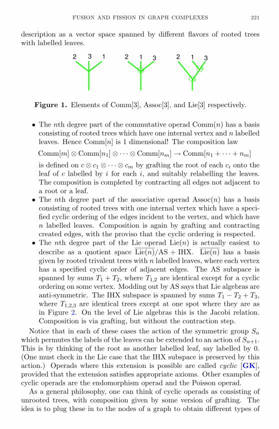
Figure 1. Elements of Comm[3], Assoc[3], and Lie[3] respectively.
• The nth degree part of the commutative operad Comm(n) has a basisconsisting of rooted trees which have one internal vertex and n labelledleaves. Hence Comm[n] is 1 dimensional! The composition law
Comm[m]⊗ Comm[n1]⊗ · · · ⊗ Comm[nm] → Comm[n1 + · · ·+ nm]
is defined on c⊗ c1 ⊗ · · · ⊗ cm by grafting the root of each ci onto theleaf of c labelled by i for each i, and suitably relabelling the leaves.The composition is completed by contracting all edges not adjacent toa root or a leaf.
• The nth degree part of the associative operad Assoc(n) has a basisconsisting of rooted trees with one internal vertex which have a speci-fied cyclic ordering of the edges incident to the vertex, and which haven labelled leaves. Composition is again by grafting and contractingcreated edges, with the proviso that the cyclic ordering is respected.
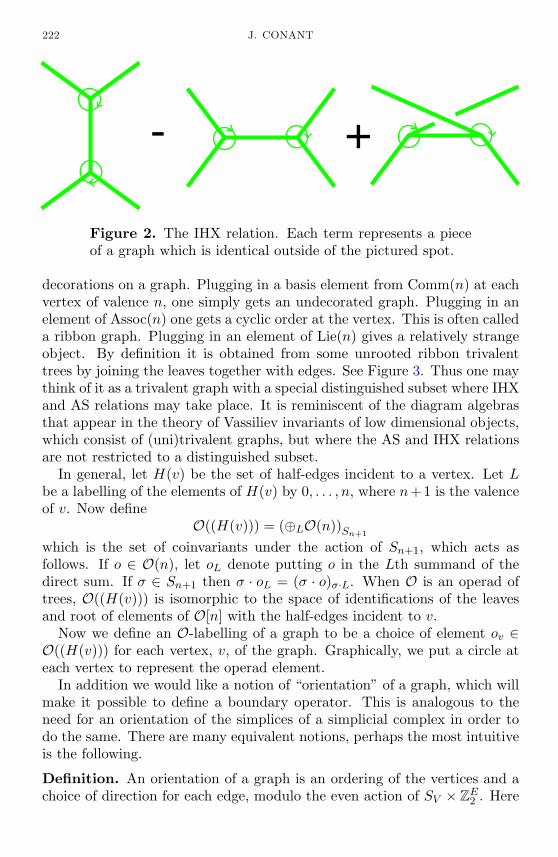
• The nth degree part of the Lie operad Lie(n) is actually easiest todescribe as a quotient space Lie(n)/AS + IHX. Lie(n) has a basisgiven by rooted trivalent trees with n labelled leaves, where each vertexhas a specified cyclic order of adjacent edges. The AS subspace isspanned by sums T1 + T2, where T1,2 are identical except for a cyclicordering on some vertex. Modding out by AS says that Lie algebras areanti-symmetric. The IHX subspace is spanned by sums T1 − T2 + T3,where T1,2,3 are identical trees except at one spot where they are asin Figure 2. On the level of Lie algebras this is the Jacobi relation.Composition is via grafting, but without the contraction step.
Notice that in each of these cases the action of the symmetric group Snwhich permutes the labels of the leaves can be extended to an action of Sn+1.This is by thinking of the root as another labelled leaf, say labelled by 0.(One must check in the Lie case that the IHX subspace is preserved by thisaction.) Operads where this extension is possible are called cyclic [GK],provided that the extension satisfies appropriate axioms. Other examples ofcyclic operads are the endomorphism operad and the Poisson operad.
As a general philosophy, one can think of cyclic operads as consisting ofunrooted trees, with composition given by some version of grafting. Theidea is to plug these in to the nodes of a graph to obtain different types of
222 J. CONANT
+-
Figure 2. The IHX relation. Each term represents a pieceof a graph which is identical outside of the pictured spot.
decorations on a graph. Plugging in a basis element from Comm(n) at eachvertex of valence n, one simply gets an undecorated graph. Plugging in anelement of Assoc(n) one gets a cyclic order at the vertex. This is often calleda ribbon graph. Plugging in an element of Lie(n) gives a relatively strangeobject. By definition it is obtained from some unrooted ribbon trivalenttrees by joining the leaves together with edges. See Figure 3. Thus one maythink of it as a trivalent graph with a special distinguished subset where IHXand AS relations may take place. It is reminiscent of the diagram algebrasthat appear in the theory of Vassiliev invariants of low dimensional objects,which consist of (uni)trivalent graphs, but where the AS and IHX relationsare not restricted to a distinguished subset.
In general, let H(v) be the set of half-edges incident to a vertex. Let Lbe a labelling of the elements of H(v) by 0, . . . , n, where n+1 is the valenceof v. Now define
O((H(v))) = (⊕LO(n))Sn+1
which is the set of coinvariants under the action of Sn+1, which acts asfollows. If o ∈ O(n), let oL denote putting o in the Lth summand of thedirect sum. If σ ∈ Sn+1 then σ · oL = (σ · o)σ·L. When O is an operad oftrees, O((H(v))) is isomorphic to the space of identifications of the leavesand root of elements of O[n] with the half-edges incident to v.
Now we define an O-labelling of a graph to be a choice of element ov ∈O((H(v))) for each vertex, v, of the graph. Graphically, we put a circle ateach vertex to represent the operad element.
In addition we would like a notion of “orientation” of a graph, which willmake it possible to define a boundary operator. This is analogous to theneed for an orientation of the simplices of a simplicial complex in order todo the same. There are many equivalent notions, perhaps the most intuitiveis the following.
Definition. An orientation of a graph is an ordering of the vertices and achoice of direction for each edge, modulo the even action of SV × ZE2 . Here

FUSION AND FISSION IN GRAPH COMPLEXES 223
V and E are the number or vertices and edges of the graph, respectively.An element of SV ×ZE2 is called even if it is a product of an even number ofelements each of which is either a transposition in Sv or an element of theform (0, . . . , 1, . . . , 0) ∈ ZE2 .
Notice that any graph has exactly two orientations. Let − indicate themap switching orientations.
Remark. Lie graphs actually have a much simpler description, because theorientations of the graph and vertices cancel out to a large degree. Namely,one can think of a Lie graph as a trivalent graph with a distinguished subfor-est, whose edges are ordered modulo even permutations. The IHX relationin the Lie operad becomes the condition that the three terms in an IHXrelation of the trivalent graph sum to zero provided the edge involved is inthe forest. This will be explained carefully in [CV2].
2.1. Chain complexes. Now for any cyclic operadO we are ready to defineO-graph complexes.
Define GOv to be the span of O-labelled oriented graphs with vertices allof valence ≥ 3, modulo the relation (G, or) = −(G,−or) and also modulomultilinearity of the O-labels. More precisely, we set
GO =
⊕(G,or)
⊗v∈V (G)
O((H(v)))
/(G, or) = −(G,−or) ,
where the direct sum is over oriented graphs with vertices of valence ≥ 3,and where V (G) is the set of vertices of G. Define GOv to be the part of GOwith v vertices.
For each edge, e, in a graph (G, or) we define contraction along that edge(G, or)e to be the graph where the two operad elements at each endpoint ofe are composed along e. The induced orientation can be fixed by assumingthat the endpoints of e are labelled 1 and 2 and the edge direction is from 1 to2. The new vertex, which results from composing the two operad elements,is labelled 1, and all other indices are reduced by 1. If e is a loop, thendefine (G, or)e = 0. In the commutative case, (G, or)e is defined by simplycontracting the edge of the (undecorated) graph. In the associative case thecyclic orders at both endpoints of an edge are joined together to give a cyclicorder at the vertex resulting from the edge collapse. For an example in theLie case, see Figure 3.
Define ∂G : GOv → GOv−1 by ∂G(G, or) =∑
e∈E(G)(G, or)e, where E(G) isthe set of edges of G.
Remark. In the simpler version of the Lie case, the boundary operator addsan edge to the forest in all possible ways, with the edge’s number comingdirectly after the edge numbers in the original forest.
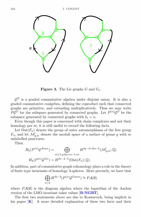
224 J. CONANT
1
2
e 1
Figure 3. The Lie graphs G and Ge.
GO is a graded commutative algebra under disjoint union. It is also agraded commutative coalgebra, defining the coproduct such that connectedgraphs are primitive, and extending multiplicatively. Thus we may writePGO for the subspace generated by connected graphs. Let P (n)GO be thesubspace generated by connected graphs with b1 = n.
Even though this paper is concerned with chain complexes and not theirhomology per se, it is still useful to record the following facts.
Let Out(Fn) denote the group of outer automorphisms of the free groupFn, and let M′
g,m denote the moduli space of a surface of genus g with munlabelled punctures.
Then
Hk(P (n)GAssoc) =⊕
m≥1,g:2g+m−1=n
H4g−4+2m−k(M′g,m; Q)
Hk(P (n)GLie) = H2n−2−k(Out(Fn); Q).
In addition, part of commutative graph cohomology plays a role in the theoryof finite type invariants of homology 3-spheres. More precisely, we have that⊕
n≥2
H2n−2(P (n)GComm) ∼= PA(∅)
where PA(∅) is the diagram algebra where the logarithm of the Aarhusversion of the LMO invariant takes values [B-NGRT].
The first two statements above are due to Kontsevich, being implicit inhis paper [K]. A more detailed explanation of these two facts and their

FUSION AND FISSION IN GRAPH COMPLEXES 225
proofs will appear in [CV2]. The last statement, the relation to finite typeinvariants, is essentially content-free, being a trivial isomorphism, at leastmodulo equivalences of various notions of orientation.
2.2. Cohomology. In at least two interesting cases, it is possible to definegraph cohomology. The coboundary operator δ is the sum of inserting anedge in all possible ways. In the commutative and associative cases thismakes perfect sense. Unfortunately, in the Lie case an insertion, which isessentially the deletion of an edge from the forest, does not preserve theIHX subspace and is not well-defined. In the cases where δ can be definedthe boundary and coboundary are adjoint with respect to the inner product〈G,H〉 = |Aut(G)|δGH . This can be seen by applying the argument of [CV],Proposition 12 mutatis mutandis.
3. Fusion.
We start with an oriented labelled 2n-gon. Label every other edge on itsperimeter consecutively by the numbers 1 . . . n, consistent with the orienta-tion. Now fix n directed edges e1, . . . , en of a graph G. Define G 〈e1, . . . , en〉to be the graph formed in the following way. First, for each i, glue the edgemarked i of the 2n-gon to the edge ei of the graph. Second, delete theseedges along which the 2n-gon was attached leaving n new edges. This isillustrated in Figure 4. The graph G 〈e1, . . . , en〉 has an induced orientationwhich can be easily described. Fix a labelling of the graph such that thedirections of the edges e1, . . . , en are both consistent with the graph’s orien-tation and with the directions which correspond to the gluing. The n newedges have orientations induced by the n-gon. Switch all of these, as is usualwith a cobordism.
G2
G1
G3
G2
G1
G3
1
2
3
G2
G1
G3
Figure 4. One term in φ3(G1, G2, G3).
Now, for any n ∈ N we define an operation
φn : SnGO → GO
by φn(G1 · · · Gn) =∑
(G1 ·G2 · · · ·Gn)〈e1, . . . , en〉e, where:
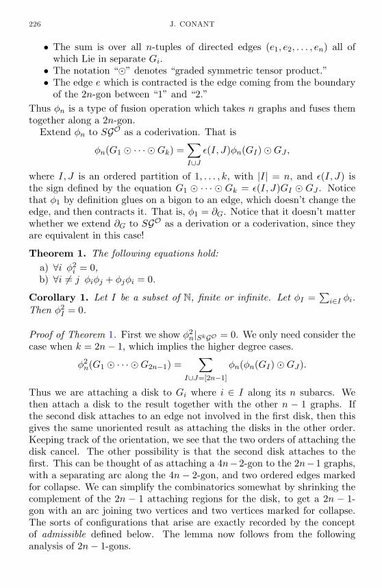
226 J. CONANT
• The sum is over all n-tuples of directed edges (e1, e2, . . . , en) all ofwhich Lie in separate Gi.
• The notation “” denotes “graded symmetric tensor product.”• The edge e which is contracted is the edge coming from the boundary
of the 2n-gon between “1” and “2.”Thus φn is a type of fusion operation which takes n graphs and fuses themtogether along a 2n-gon.
Extend φn to SGO as a coderivation. That is
φn(G1 · · · Gk) =∑I∪J
ε(I, J)φn(GI)GJ ,
where I, J is an ordered partition of 1, . . . , k, with |I| = n, and ε(I, J) isthe sign defined by the equation G1 · · · Gk = ε(I, J)GI GJ . Noticethat φ1 by definition glues on a bigon to an edge, which doesn’t change theedge, and then contracts it. That is, φ1 = ∂G. Notice that it doesn’t matterwhether we extend ∂G to SGO as a derivation or a coderivation, since theyare equivalent in this case!
Theorem 1. The following equations hold:a) ∀i φ2
i = 0,b) ∀i 6= j φiφj + φjφi = 0.
Corollary 1. Let I be a subset of N, finite or infinite. Let φI =∑
i∈I φi.Then φ2
I = 0.
Proof of Theorem 1. First we show φ2n|SkGO = 0. We only need consider the
case when k = 2n− 1, which implies the higher degree cases.
φ2n(G1 · · · G2n−1) =
∑I∪J=[2n−1]
φn(φn(GI)GJ).
Thus we are attaching a disk to Gi where i ∈ I along its n subarcs. Wethen attach a disk to the result together with the other n − 1 graphs. Ifthe second disk attaches to an edge not involved in the first disk, then thisgives the same unoriented result as attaching the disks in the other order.Keeping track of the orientation, we see that the two orders of attaching thedisk cancel. The other possibility is that the second disk attaches to thefirst. This can be thought of as attaching a 4n−2-gon to the 2n−1 graphs,with a separating arc along the 4n− 2-gon, and two ordered edges markedfor collapse. We can simplify the combinatorics somewhat by shrinking thecomplement of the 2n − 1 attaching regions for the disk, to get a 2n − 1-gon with an arc joining two vertices and two vertices marked for collapse.The sorts of configurations that arise are exactly recorded by the conceptof admissible defined below. The lemma now follows from the followinganalysis of 2n− 1-gons.

FUSION AND FISSION IN GRAPH COMPLEXES 227
Define Conf(2n−1, n) be the set of admissible configurations of a 2n−1-gon. An admissible configuration consists of an embedded arc on the 2n−1-gon between two of the vertices, thereby partitioning the 2n−1 vertices intotwo sets of n− 1 and n− 2 respectively, on each side of the arc. There arealso two vertices labelled by 1 and 2, the 1 must be in the set of n − 1and the 2 must be among the n − 2 or it could be one of the endpointsof the arc. We claim that the subset of Conf(2n − 1, n) where two specificvertices are marked 1 and 2 is bijective with the subset where these verticesare marked 2 and 1, respectively. This follows from the fact that thereis a unique automorphism exchanging any two vertices of a 2n − 1-gon.This induces a bijection between the two types of configurations. Keepingtrack of orientations, we see that the terms of corresponding to elements ofConf(2n− 1, n) cancel in pairs.
The fact that φi, φj anti-commute follows from the following similar factsabout configurations of i+ j − 1-gons, Conf(i+ j − 1, i, j). The arc in thiscase will partition the vertices into a set of i− 1, and a set of j − 2, wherethe 1 vertex must Lie in the i− 1 and the 2 elsewhere. We claim there is abijective correspondence between subsets of Conf(i + j − 1, i, j) where twofixed vertices are labelled 1 and 2 and the subsets of Conf(i + j − 1, j, i)where these vertices are labelled 2 and 1. To see this, fix an automorphismof the i+ j − 1-gon, exchanging the two given vertices. This will carry oneset of configurations onto the other.
Proposition 1. φn is canonically zero at the level of homology.
Proof. The fact that φn is even compatible with homology is the fact
∂G φn + φn ∂G = 0
where ∂G is extended to SGO as a derivation. This follows since ∂G = φ1.It remains to show that it vanishes canonically. Consider the map
µn : SnGO → GO
which is defined by gluing in a 2n-gon in all possible ways, but withoutcontracting an edge. Then a straightforward argument shows that φn =∂Gµn − µn∂G. Thus if the input to φn consists of n cycles, the µn∂G termin this equation vanishes, and what is left expresses φn as a boundary.
4. Fission.
In this section, for simplicity, we restrict ourselves to connected graphs,although much of it can be generalized to the nonconnected case. In partic-ular, when edge insertions make sense, one can dualize and prove Theorem 2analogously to Proposition 11 of [CV].
Note that GO ∼= S(PGO). Denote this isomorphism by S. Let
πi : S(PGO) → Si(PGO)

228 J. CONANT
be the natural projection. Define the map
∂i : GOv → GOv−1
by summing over all ways of attaching a 2i-gon to the edges of an O-graph,and then contracting the edge between 1 and 2. The behavior of this opera-tor (which does not have square zero) is complicated, but it becomes betterbehaved if we look at the part which disconnects the graph the most.
Definition. The mapθi : PGO → Si(PGO)
is defined as the composition 12πi S ∂i.
The operator θi can be thought of as a type of fission, where a graphsplits up into i particles. See Figure 5.
1
2
3
G2
G1
G3
G1G3
G2
G2
G1
G3
Figure 5. A term in θ3(G). The middle picture representsa term in ∂3(G), and the final picture is a result of applyingS.
Extend θi toθi : S(PGO) → S(PGO)
as a derivation. Notice that θ1 = ∂G = φ1.
Theorem 2. The following identities hold:a) ∀i 6= j θiθj + θjθj = 0,b) ∀i θ2
i = 0.
Proof. We prove a). Statement b) is similar. We show that
θiθj + θjθi : GO → Si+j(GO)
is zero, which is enough. If the i-gon and j-gon attach to two different sets ofedges, they can be applied in either order to get the same (unoriented) result.Keeping track of orientation, one sees that they anticommute. Attaching onedisk, and then the other to an edge of the original disk is the same as addinga bigger disk with an ordered pair of two sides marked for collapse. We maynow apply our analysis from the proof of Theorem 1 to show that the termscancel in pairs.

FUSION AND FISSION IN GRAPH COMPLEXES 229
Corollary 2. Let I be a subset of N, finite or infinite. Let θI =∑
i∈I θi.Then θ2
I = 0.
Proposition 2. θi is canonically zero at the level of homology.
Proof. That θi is compatible with homology follows since θ1 = ∂G.A similar argument to Proposition 1 shows that θi vanishes canonically
on homology.
The operator θi can be defined for disconnected graphs as well, as wealluded to earlier. Suppose we start with a graph with k connected compo-nents. A 2i-gon attaches to one of these and it fissions into i components.In order to get a well-defined map, the remaining k−1 components must bedistributed with the i fission components in all possible ways, which leadsto more complicated formulas.
5. Compatibility.
It is unclear if there is a theory of Lie∞ bialgebras; a search of MathSciNetyields no hits. Under some obvious generalizations of the definition of Liebialgebra to the case of higher order operations on the symmetric algebra,the higher degree fusion operations are not compatible with the higher degreefission operations. Interestingly, degree 2 fission is compatible with degree2 fusion on the subcomplex of connected graphs with no separating edges.As was noted in [CV] this is not the case on the full complex GO.
Definition. Let P irredGO be the subcomplex of GO spanned by connected(primitive) graphs with no separating edges (irreducible).
Theorem 3. On P irredGO the following equation holds:
θ2φ2(X Y ) + φ2(θ2(X) Y ) + (−1)xφ2(X θ2(Y )) = 0.
Proof. The bracket φ2 and cobracket θ2 coincide with the operations [·, ·] andθ defined in [CV] for the commutative operad. In that paper, we definedeverything in terms of contracting pairs of half-edges, but the operationsare easily seen to match. (In fact, we mentioned a “dotted line notation” inthat paper which is very close to the definition of φ2 considered here.) Nowuse the argument from [CV] Theorem 1, which holds even if the vertices arelabelled by the operad O.
Acknowledgements. It is a pleasure to thank Karen Vogtmann for manydiscussions. I also wish to thank Swapneel Mahajan for his perceptive input.Credit also goes to the anonymous referee who noticed an error in the originalmanuscript and suggested many expositional improvements.
230 J. CONANT
References
[B-NGRT] D. Bar-Natan, S. Garoufalidis, L. Rozansky and D.P. Thurston, The Aarhusintegral of rational homology 3-spheres I: A highly nontrivial flat connectionon S3, to appear in Selecta Mathematica, see also q-alg/9706004.
[C] M. Chas, Combinatorial Lie bialgebras of curves on surfaces. Preprint 2001,math.GT/0105178.
[CS] M. Chas and D. Sullivan, String topology. Preprint 1999, math.GT/9911159.
[CS2] , Lie bialgebras of closed strings in manifolds. Preprint.
[CV] J. Conant and K. Vogtmann, Infinitesimal operations on graph complexes.Preprint, math.QA/0111198.
[CV2] , in preparation.
[CuV] M. Culler and K. Vogtmann, Moduli of graphs and automorphisms of freegroups, Invent. Math., 84(1) (1986), 91-119, MR 87f:20048, Zbl 0589.20022.
[GK] E. Getzler and M. Kapranov, Cyclic operads and cyclic homology, Geometry,Topology, and Physics, 167-201, Conf. Proc. Lecture Notes Geom. Topology,IV, Internat. Press, Cambridge, MA, 1995, MR 96m:19011, Zbl 0883.18013.
[GK2] , Modular operads, Compositio Math., 110(1) (1998), 65-126,MR 99f:18009, Zbl 0894.18005.
[K] M. Kontsevich, Formal (non)commutative symplectic geometry, The GelfandMathematical Seminars, 1990-1992, 173-187, Birkhauser Boston, Boston, MA,1993, MR 94i:58212, Zbl 0821.58018.
[M] M. Markl, Cyclic operads and homology of graph complexes, Rendicontidel Circolo Matematico di Palermo Serie II, Suppl., 59 (1999), 161-170,MR 2000g:18009, Zbl 0970.18011.
[MSS] M. Markl, S. Shnider and J. Stasheff, Operads in Algebra, Topology andPhysics, Mathematical Surveys and Monographs, 96, American Mathemat-ical Society, 2002, CMP 1 898 414.
[P] R.C. Penner, Perturbative series and the moduli space of Riemann surfaces, J.Differential Geom., 27(1) (1988), 35-53, MR 89h:32045, Zbl 0608.30046.
[V] A. Voronov, Notes on universal algebra. Preprint, math.QA/0111009.
Received April 4, 2002 and revised July 25, 2002. This work was partially supported byNSF VIGRE grant DMS-9983660.
Department of MathematicsCornell UniversityIthaca, NY 14853-4201E-mail address: [email protected]

PACIFIC JOURNAL OF MATHEMATICSVol. 209, No. 2, 2003
SOME PLANAR ALGEBRAS RELATED TO GRAPHS
Brian Curtin
Let X denote a finite nonempty set, and let W denote amatrix whose rows and columns are indexed by X and whoseentries belong to some field K. We study three planar algebrasrelated to W . Briefly, a planar algebra is a graded vectorspace V = ∪n∈Z+∪+, −Vn which is closed under “planar”operators.
The first planar algebra which we study, FW = ∪FWn , is
defined by the group theoretic properties of W . For n ∈ Z+,FW
n is the vector space of functions from Xn to K which areconstant on the Aut(W )-orbits of Xn, and FW
+ , FW− are iden-
tified with K. The second planar algebra, PW = ∪PWn , is the
planar algebra generated W . We define it combinatorially:PW
n is spanned by functions from Xn to K defined via sta-tistical mechanical sums on certain planar open graphs. Thethird planar algebra, OW = ∪OW
n , differs from PW only inthat the open graphs defining the functions need not be pla-nar.
It turns out that PW ⊆ OW ⊆ FW . We show that PW =OW if and only if PW
4 contains a single special function knownas the “transposition”. We show that OW = FW whenever|X|! is not divisible by the characteristic of K.
1. Introduction.
Planar algebras were introduced by V.F.R. Jones [15] to study the structureof subfactors. A planar algebra is a graded vector space V = ∪n∈Z+∪+,−Vnover some field K which is closed under certain operators. True to its op-erator algebra origins, an emphasis is placed upon the interactions of theoperators. These operators are defined diagrammatically by objects knownas planar tangles. We recall relevant definitions in Section 2. The study ofa planar algebra via the dependencies of these operators has a knot theo-retic flavor, very much like Conway’s tangles and skein relations [4]. This isno coincidence, as planar algebras were influenced by the deep relationshipbetween subfactors and knots [12] and [14].
When dimVn is finite for all n, it is natural to ask for the exact value.We shall consider this problem for some combinatorial planar algebras. Inour examples, Vn is a vector space of functions from Xn to K for some fixed,
231
232 BRIAN CURTIN
finite, nonempty set X. The action of the planar tangles is defined via thestatistical mechanical construction known as a partition function.
In Section 3 we introduce three planar algebras related to a matrix Wwhose rows and columns are indexed by X and entries are in K. In thefirst planar algebra defined from W , FW = ∪FW
n , the vector space FWn
consists of those functions from Xn to K which are constant on the orbitsof Xn under the action of Aut(W ). The second is a singly generated planaralgebra, PW = ∪PWn , whose vector space PWn is spanned by functions fromXn to K defined via statistical mechanical state sums on the planar graphsderived from planar tangles. The third planar algebra, OW = ∪OW
n , differsfrom PW only in that the graphs defining the functions need not be planar.
It turns out that PWn ⊆ OWn ⊆ FW
n . It is easy to compute dimFWn using
the Cauchy-Frobenius-Burnside formula for group characters. However, weare more interested in dimPWn , and it is generally very difficult to compute.Thus we consider when PWn = FW
n for all n. The planar algebra OW playsan important role in this problem. In Section 4, we show that PW = OW ifand only if PW4 contains a particular element called the “transposition”. Theproof of this result is essentially skein theoretic in nature. Then in Section 5,show that OW = FW whenever |X|! is not divisible by the characteristicof K. Since this condition holds in characteristic zero, the most importantcase is thus treated. To prove this result, we encode OW
n into polynomialsand then appeal to results concerning the polynomial invariants of a finitegroup.
These results are related to Theorem 4.3 of [16] concerning a certainplanar algebra Pσ which contains PW . This result asserts that any planarsubalgebra of Pσ which contains a transposition is the set of elements ofPσ which are fixed under the action of some group G such that Aut(W ) ⊆G ⊆ SX . This result relies on the theory of subfactors, and so it is onlyapplicable when the ground field is the real or complex numbers and whenthe matrix W is symmetric. By introducing the intermediate planar algebraOW we have extended this result (as applied to PW ) to almost any field andto any matrix. In this case we also know precisely which group is involved.Moreover, the proof given here is combinatorial in nature, where the originalwas very non-combinatorial.
2. Planar algebras: Definitions.
Planar algebras were introduced to study the structure of subfactors. Trueto their operator algebra origins, planar algebras are defined in terms ofoperators on vector spaces. These operators are defined diagrammatically byobjects known as planar tangles. A planar tangle can be presented in severalways. We shall use a slight variation of the operadic definition of [15] (seealso [16]). From this point of view, a planar tangle consists of a collection

GRAPHICAL PLANAR ALGEBRAS 233
of disjoint disks which are joined by disjoint smooth curves, together with acoloring of the regions formed by the strings and disks. Various constraintson this collection arise from their subfactor origins; however, no knowledgeof subfactors is necessary to proceed.
We begin with a definition of a planar tangle. Let D0 denote the unitdisk. Pick disjoint disks D1, D2, . . . , Dn in the interior of D0. Form afinite collection of disjoint “strings” (simple smooth curves) in the interiorof D0\ ∪ni=1 Di, all of whose endpoints meet the boundary of some disktransversally. There may be some closed loops which touch no disk. Furtherassume that an even number of strings touch each disk, say 2ki touching Di.Color the regions interior to D0\ ∪ni=1 Di formed by the strings black andwhite so that regions on either side of a string have opposite colors. Callthe points on the boundary of each disk where a string touches “marked”.The marked points divide the boundary of each disk into intervals. Oneach disk, one of the intervals which touches a white region is chosen tobe “privileged”. The entire boundary of a disk with no marked points iseither privileged or not according to whether it touches a white region ora black region. Specifying the privileged intervals makes the coloring dataredundant. It will sometimes be convenient to number the marked pointson each disk consecutively in a clockwise direction where the marked pointat the clockwise end of the privileged interval is numbered one.
The smooth isotopy class of this collection of disks, strings, coloring,and privileged intervals is called a planar k0-tangle. There is a naturalcomposition for planar tangles. If S is a planar k-tangle with an internaldisk Di with 2ki marked points and T is a planar ki-tangle, then we mayreplace Di with a rescaled and isotoped version of T without its unit disk, bymatching corresponding marked points (first to first, etc.) and smoothingthe connections of the strings. The coloring conventions are preserved bycomposition. The collection of planar tangles with this composition is calledthe planar operad.
A general planar algebra is a graded vector space Vk for k > 0 and twovector spaces V+ and V− such that every element T of the planar operaddetermines a multilinear map from a tensor product of these vector spaces,one for each internal disk of T , to the vector space corresponding to theboundary of T . We require a natural homomorphism property. Given planartangles T1, T2, T3 which admit compositions of T2 into T1 and T3 into thiscomposition, the net result of these compositions in the planar operad doesnot depend upon the order in which they are carried out: The same mustbe true for the corresponding multilinear maps on the planar algebra. Wealso impose a condition on V+ and V−. We view these two vector spacesas corresponding to the two colorings of any planar 0-tangle–V+ to thosecolored black next to the unit disk and V− to those colored white nextto the unit disk. Observe that surrounding the interior component with a

234 BRIAN CURTIN
closed string reverses its coloring. We require that surrounding the interiorcomponents of a planar 0-tangle with two closed strings yields a multilinearmap to V+ or V− which differs from the original multilinear map only by afixed scalar multiple.
Let V denote a planar algebra. Then V is said to be finite dimensionalwhenever the vector spaces V+, V−, and Vk (k > 0) are all finite dimensional.All of the examples that we shall consider in this paper are finite dimensional.In fact, V+ and V− will both be one-dimensional, making the examplesplanar algebras in the sense of [15]. Given that V is finite dimensional, it isnatural to compute dimVk for all k. This problem motivates the results ofthis paper. We are interested in a singly generated planar algebra PW whichis contained in a planar algebra FW whose dimensions we can compute. Weshall consider when these two planar algebras are equal. We now describethe planar algebras which we shall study.
3. Planar algebras: Examples.
3.1. The planar algebra of functions on a finite set. We present avery simple planar algebra. We are more interested in some of its planarsubalgebras, but we take this opportunity to describe the multilinear mapcorresponding to each planar tangle with no other distractions. This corre-spondence will be the same in all planar algebras which follow.
Let X denote a finite, nonempty set, and let K denote a field. For eachpositive integer k, let Xk be the vector space of all functions from Xk toK (k > 0), with X+, X− identified with K. Then X = ∪Xk is a planaralgebra. Let T denote a planar k0-tangle with internal disks D1, D2, . . . ,Dn with respectively 2k1, 2k2, . . . , 2kn many marked points. Then T definesa multilinear map
⊗ni=1Xki
→ Xk0 as follows. Index the black regions of Tby 1, 2, . . . , m. For all i (0 ≤ i ≤ n) and for all j (1 ≤ j ≤ ki), let Sij bethe index of the jth black incident with Di when traversing the boundary ofDi clockwise so that the privileged interval is traversed last. Given fi ∈ Xki
(1 ≤ i ≤ n), define a function Z(f1,f2,...,fn)T : Xk0 → C which, when evaluated
at (x1, x2, . . . , xk0), returns∑σ
∏n
i=1fi(σ(Si1), σ(Si2), . . . , σ(Siki
)),(1)
where σ runs over all maps from 1, 2, . . . ,m to X with σ(S0j) = xj .Extend ZT multilinearly to a map
⊗ni=1Xi → Xk0 . The homomorphism
property of planar algebras follows since the function only depends uponthe incidences of the black regions and composition merges regions with thesame color. Enclosing a planar 0-tangle with two closed strings preserves thecolor of the interior (reverses it twice) but adds an isolated black band. Thismodified tangle gives a multilinear map which is |X| times the multilinearmap corresponding to the original tangle. Thus X is a planar algebra.

GRAPHICAL PLANAR ALGEBRAS 235
3.2. Planar algebras constructed via finite group action. Let Xdenote a finite, nonempty set. Let SX denote the symmetric group onX. For each positive integer k, extend the action of SX to Xk in thenatural fashion: For all g ∈ SX and for all (x1, x2, . . . , xk) ∈ Xk, letg(x1, x2, . . . , xk) = (g(x1), g(x2), . . . , g(xk)). Let G ⊆ SX denote a sub-group so that G is a permutation group on X. By a G-orbit of Xk, we meana nonempty subset Y ⊆ Xk such that ~x, ~y ∈ Y if and only if there existsg ∈ G such that ~x = g(~y).
Let K denote a field. For each positive integer k, let Fk(G, X) denotethe vector space of functions from Xk → K which depend only upon the G-orbit of their inputs. We identify the vector spaces F+(G, X) and F−(G, X)with the field K (constant functions). Together, these vector spaces forma planar algebra F(G, X) with the same planar structure as X. That isto say, (1) defines a map
⊗ni=1Fki
(G, X) → Fk0(G, X). To see that thisis so, pick fi ∈ Fki
(G, X) (1 ≤ i ≤ n), and define f0 : Xk0 → K by (1).To see that f0 is constant on each G-orbit of Xk0 , consider replacing eachmap σ in (1) by g σ. The effect of this change on the boundary leads (1)to return f0(gx1, gx2, . . . , gxk0) = f0(x1, x2, . . . , xk0) since fi ∈ Fki
(G, X)(1 ≤ i ≤ n). Thus f0 ∈ Fk0(G, X). Hence F(G, X) = ∪Fk(G, X) is a planaralgebra. F(G, X) is called the fixed-point planar algebra of G acting on X.This planar algebra is discussed in [15].
The vector spaces of Fk(G, X) are finite dimensional, and their dimensioncan be computed via the Cauchy-Frobenius-Burnside formula for the char-acters of the group, which we briefly recall now. See [11], for example. Thepermutation representation of G acting on X is the map g 7→ R(g) ∈MX(C)with (x, y)-entry equal to 1 if y = g · x and 0 otherwise (x, y ∈ X). Thepermutation character of G acting on X is the map π : G → C given byπ(g) = Tr R(g) (g ∈ G). Fix a positive integer k. Then the number oforbits of Xk under the action of G is
dimFk(G, X) =1|G|
∑g∈G
(π(g))k.(2)
3.3. A planar algebra PW . Fix a field K. Let X denote a finite, non-empty set. Let MX(K) denote the set of matrices with rows and columnsindexed byX and entries in K. PickW ∈MX(K). Given k > 0, we describea rule using W which maps any planar k-tangle all of whose internal diskshave exactly 4 marked points to a function Xk → C. The vector space PWkspanned by these functions will be part of the grading of a planar algebraPW . A similar rule gives the vector spaces PW+ and PW− , which turn out tobe isomorphic to K.
Let T denote planar k-tangle in the unit disk D0 with n internal disksD1, D2, . . . , Dn each having exactly 4 marked points. As in Subsection3.1, label the black regions of T with indices 1, 2, . . . , m and for all i

236 BRIAN CURTIN
(0 ≤ i ≤ n) and for j = 1, 2, let Sij denote the index of the jth black regionincident with Di when traversing the boundary of Di clockwise so that theprivileged interval is traversed last. Define a function ZWT : Xk → K which,when evaluated at (x1, x2, . . . , xk), returns
ZWT (x1, x2, . . . , xk) =∑σ
n∏i=1
W (σ(Si1), σ(Si2)),(3)
where σ runs over all maps from 1, 2, . . . ,m to X with σ(S0j) = xj . LetPWk denote the K-linear span of all functions which arise in this fashion froma planar k-tangle. For k = 0, we use the same rule to define functions, butplace them in PW+ or PW− when the color of the 0-tangle near the unit circleis black or white, respectively.
Now PW = ∪PWn is a planar subalgebra of X with closure under (1) as-sured since the composition of planar tangles yields a planar tangle. Theplanar algebra PW is called the planar algebra generated by W . This pla-nar algebra is also discussed in [15]. Singly generated planar algebras areconsidered in [3] as well. Not all of the planar algebras considered in [3] aregenerated by a matrix, however.
By an automorphism of W , we mean a permutation s of X such thatW (u, v) = W (s(u), s(v)) for all u, v ∈ X. Let Aut(W ) denote the fullgroup of automorphisms of W . Observe that PW ⊆ F(Aut(W ), X) sincethe definition of the functions in PW depend only upon the structure ofW . Thus (2) gives an upper bound for dimPWk . Our main result concernsthe case of equality. The proof compares PW and F(Aut(W ), X) to anintermediate planar algebra which we now describe.
3.4. A planar algebra OW . We use the language of graph theory togeneralize the construction of PW of the previous subsection. We beginwith some graph theoretic terminology.
By a multi-digraph, we mean a pair ∆ = (V,E), where V is a nonemptyset and E is a multiset of ordered pairs of (not necessarily distinct) elementsof V . Let ∆ = (V,E) be a multi-digraph. The elements of V are called thevertices of ∆, and an ordered pair (u, v) ∈ E is called a (directed) edgefrom u to v. We say that there are multiple edges from u to v whenever themultiset E contains two or more copies of (u, v). Throughout this paper weshall assume that all multi-digraphs have finite vertex and edge sets. Fixa nonnegative integer n. By an open graph of boundary size n, we mean atriple Γ = (V,E,~b), where (V,E) is a multi-digraph and ~b is an n-tuple ofelements of V , called the boundary vector of the open graph. Let On denotethe set of all open graphs of boundary size n.
Let Γ = (V,E,~b) denote an open graph of boundary size n. Γ is said tobe planar if the multi-digraph (V,E) has a plane embedding (no crossingedges) into the interior of an n-gon with clockwise ordered vertices b′1, b
′2,
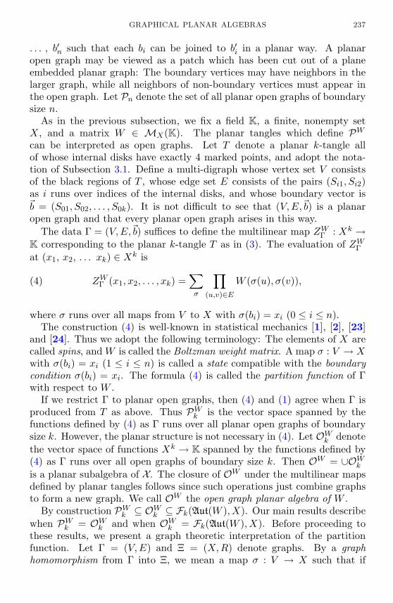
GRAPHICAL PLANAR ALGEBRAS 237
. . . , b′n such that each bi can be joined to b′i in a planar way. A planaropen graph may be viewed as a patch which has been cut out of a planeembedded planar graph: The boundary vertices may have neighbors in thelarger graph, while all neighbors of non-boundary vertices must appear inthe open graph. Let Pn denote the set of all planar open graphs of boundarysize n.
As in the previous subsection, we fix a field K, a finite, nonempty setX, and a matrix W ∈ MX(K). The planar tangles which define PWcan be interpreted as open graphs. Let T denote a planar k-tangle allof whose internal disks have exactly 4 marked points, and adopt the nota-tion of Subsection 3.1. Define a multi-digraph whose vertex set V consistsof the black regions of T , whose edge set E consists of the pairs (Si1, Si2)as i runs over indices of the internal disks, and whose boundary vector is~b = (S01, S02, . . . , S0k). It is not difficult to see that (V,E,~b) is a planaropen graph and that every planar open graph arises in this way.
The data Γ = (V,E,~b) suffices to define the multilinear map ZWΓ : Xk →K corresponding to the planar k-tangle T as in (3). The evaluation of ZWΓat (x1, x2, . . . xk) ∈ Xk is
ZWΓ (x1, x2, . . . , xk) =∑σ
∏(u,v)∈E
W (σ(u), σ(v)),(4)
where σ runs over all maps from V to X with σ(bi) = xi (0 ≤ i ≤ n).The construction (4) is well-known in statistical mechanics [1], [2], [23]
and [24]. Thus we adopt the following terminology: The elements of X arecalled spins, and W is called the Boltzman weight matrix. A map σ : V → Xwith σ(bi) = xi (1 ≤ i ≤ n) is called a state compatible with the boundarycondition σ(bi) = xi. The formula (4) is called the partition function of Γwith respect to W .
If we restrict Γ to planar open graphs, then (4) and (1) agree when Γ isproduced from T as above. Thus PWk is the vector space spanned by thefunctions defined by (4) as Γ runs over all planar open graphs of boundarysize k. However, the planar structure is not necessary in (4). Let OW
k denotethe vector space of functions Xk → K spanned by the functions defined by(4) as Γ runs over all open graphs of boundary size k. Then OW = ∪OW
k
is a planar subalgebra of X. The closure of OW under the multilinear mapsdefined by planar tangles follows since such operations just combine graphsto form a new graph. We call OW the open graph planar algebra of W .
By construction PWk ⊆ OWk ⊆ Fk(Aut(W ), X). Our main results describe
when PWk = OWk and when OW
k = Fk(Aut(W ), X). Before proceeding tothese results, we present a graph theoretic interpretation of the partitionfunction. Let Γ = (V,E) and Ξ = (X,R) denote graphs. By a graphhomomorphism from Γ into Ξ, we mean a map σ : V → X such that if
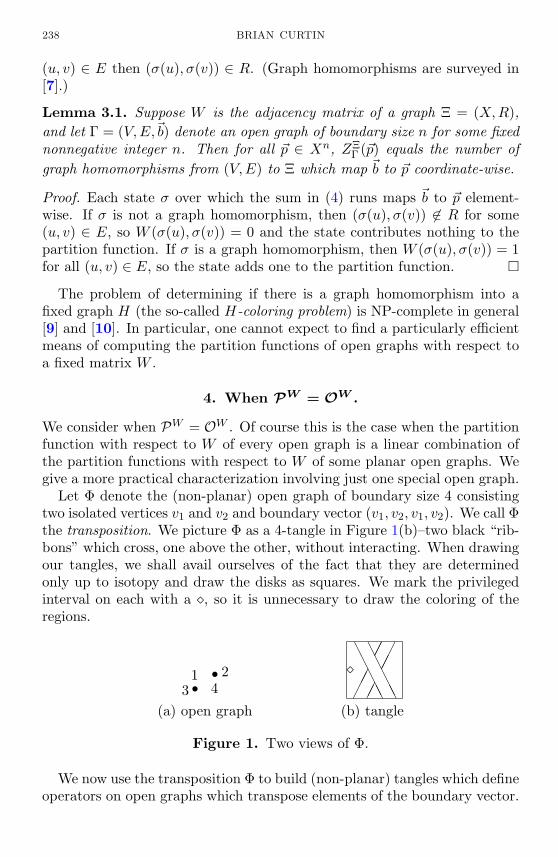
238 BRIAN CURTIN
(u, v) ∈ E then (σ(u), σ(v)) ∈ R. (Graph homomorphisms are surveyed in[7].)
Lemma 3.1. Suppose W is the adjacency matrix of a graph Ξ = (X,R),and let Γ = (V,E,~b) denote an open graph of boundary size n for some fixednonnegative integer n. Then for all ~p ∈ Xn, ZΞ
Γ (~p) equals the number ofgraph homomorphisms from (V,E) to Ξ which map ~b to ~p coordinate-wise.
Proof. Each state σ over which the sum in (4) runs maps ~b to ~p element-wise. If σ is not a graph homomorphism, then (σ(u), σ(v)) 6∈ R for some(u, v) ∈ E, so W (σ(u), σ(v)) = 0 and the state contributes nothing to thepartition function. If σ is a graph homomorphism, then W (σ(u), σ(v)) = 1for all (u, v) ∈ E, so the state adds one to the partition function.
The problem of determining if there is a graph homomorphism into afixed graph H (the so-called H-coloring problem) is NP-complete in general[9] and [10]. In particular, one cannot expect to find a particularly efficientmeans of computing the partition functions of open graphs with respect toa fixed matrix W .
4. When PW = OW .
We consider when PW = OW . Of course this is the case when the partitionfunction with respect to W of every open graph is a linear combination ofthe partition functions with respect to W of some planar open graphs. Wegive a more practical characterization involving just one special open graph.
Let Φ denote the (non-planar) open graph of boundary size 4 consistingtwo isolated vertices v1 and v2 and boundary vector (v1, v2, v1, v2). We call Φthe transposition. We picture Φ as a 4-tangle in Figure 1(b)–two black “rib-bons” which cross, one above the other, without interacting. When drawingour tangles, we shall avail ourselves of the fact that they are determinedonly up to isotopy and draw the disks as squares. We mark the privilegedinterval on each with a , so it is unnecessary to draw the coloring of theregions.
s31 s
42
AAAAA
AAAAA
(a) open graph (b) tangle
Figure 1. Two views of Φ.
We now use the transposition Φ to build (non-planar) tangles which defineoperators on open graphs which transpose elements of the boundary vector.
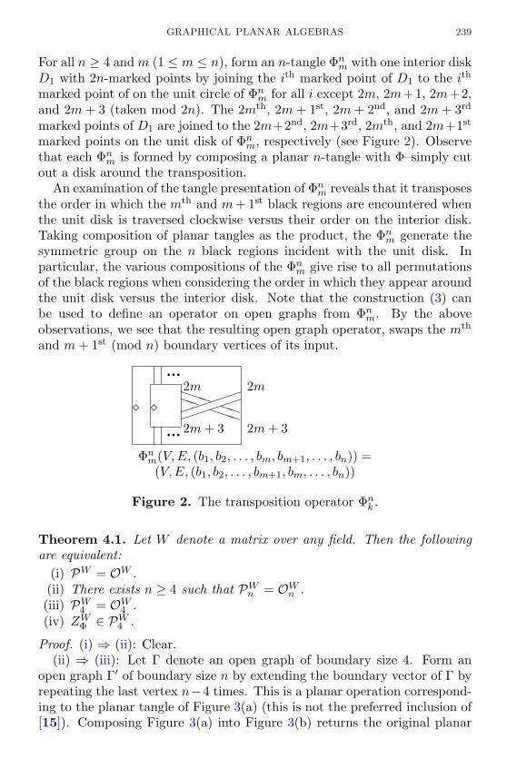
GRAPHICAL PLANAR ALGEBRAS 239
For all n ≥ 4 andm (1 ≤ m ≤ n), form an n-tangle Φnm with one interior disk
D1 with 2n-marked points by joining the ith marked point of D1 to the ith
marked point of on the unit circle of Φnm for all i except 2m, 2m+1, 2m+2,
and 2m+ 3 (taken mod 2n). The 2mth, 2m+ 1st, 2m+ 2nd, and 2m+ 3rd
marked points of D1 are joined to the 2m+2nd, 2m+3rd, 2mth, and 2m+1st
marked points on the unit disk of Φnm, respectively (see Figure 2). Observe
that each Φnm is formed by composing a planar n-tangle with Φ–simply cut
out a disk around the transposition.An examination of the tangle presentation of Φn
m reveals that it transposesthe order in which the mth and m+ 1st black regions are encountered whenthe unit disk is traversed clockwise versus their order on the interior disk.Taking composition of planar tangles as the product, the Φn
m generate thesymmetric group on the n black regions incident with the unit disk. Inparticular, the various compositions of the Φn
m give rise to all permutationsof the black regions when considering the order in which they appear aroundthe unit disk versus the interior disk. Note that the construction (3) canbe used to define an operator on open graphs from Φn
m. By the aboveobservations, we see that the resulting open graph operator, swaps the mth
and m+ 1st (mod n) boundary vertices of its input.
q q q2m+ 3 2m+ 3PP
PPP
PPPPP
2m 2m
q q qΦnm(V,E, (b1, b2, . . . , bm, bm+1, . . . , bn)) =(V,E, (b1, b2, . . . , bm+1, bm, . . . , bn))
Figure 2. The transposition operator Φnk .
Theorem 4.1. Let W denote a matrix over any field. Then the followingare equivalent:
(i) PW = OW .(ii) There exists n ≥ 4 such that PWn = OW
n .(iii) PW4 = OW
4 .(iv) ZWΦ ∈ PW4 .
Proof. (i) ⇒ (ii): Clear.(ii) ⇒ (iii): Let Γ denote an open graph of boundary size 4. Form an
open graph Γ′ of boundary size n by extending the boundary vector of Γ byrepeating the last vertex n−4 times. This is a planar operation correspond-ing to the planar tangle of Figure 3(a) (this is not the preferred inclusion of[15]). Composing Figure 3(a) into Figure 3(b) returns the original planar

240 BRIAN CURTIN
tangle along with some closed loops with white interiors, which can be re-moved with no effect in our planar algebra. By (ii), there exist open graphsΓ1, Γ2, . . . , Γk ∈ Pn such that ZWΓ′ =
∑kj=1 αjZ
WΓj
for some scalars αj . Thesame is true of Γ since we may apply the restriction to these functions.
q q q qqqq q q
q q qq q q q q q
(a) An inclusion (b) Its inverse restriction
Figure 3. Two planar tangles.
(iii) ⇒ (iv): Clear.(iv) ⇒ (i): Fix a nonnegative integer n and pick Γ ∈ On. We shall show
that there are open graphs Γ1, Γ2, . . . , Γk ∈ Pn such that ZWΓ =∑k
j=1 αjZWΓj
for some scalars αj . This will prove that OWn = PWn .
In order for an open graph to be planar, it must be possible to embed it inthe plane so that the positions of its boundary vertices are incident with theexterior and ordered clock-wise as they appear in the boundary vector. Thismay not be the case for Γ. However, by permuting the boundary vector thiscan be corrected. By (iv) and the remarks at the beginning of the section,there exist transposition operators such that
Γ = Φnm1
(Φnm2
(. . .Φnmj
(Γ) . . . )),
where Γ is an open graph with the same vertex and edge sets as Γ andboundary vector a re-ordering of that of Γ so that all repetitions occur incyclically successive positions. It is now possible to embed Γ with the desiredboundary property. There remains the possibility that Γ has crossing edgesin any plane embedding with the boundary vertices incident with the exteriorface.
In light of (iv), we now only need to prove that ZWΓ
∈ PWn . Indeed,suppose that this is the case. Then there exists a set of planar open graphsΓ1, Γ2, . . . , Γ such that ZW
Γ=
∑i=1 βjZ
WΓi
. Now by (iv) there exists a set
of planar open graphs Γ1, Γ2, . . . , Γe such that
ZWΦn
mj(Γi)
=e∑`=1
ZWeΓ`∈ PWn .
Proceeding by induction, we find that ZWΓ ∈ PWn .To show that ZW
Γ∈ PWn , it is enough to show that ZW∆ ∈ PWn for any open
graph ∆ whose boundary vector is such that all repetitions occur in cyclically

GRAPHICAL PLANAR ALGEBRAS 241
successive positions. Embed ∆ in the plane such that all of its vertices lieevenly spaced on a circle and its boundary vertices are ordered clock-wiseas they appear in the boundary vector. If no edges cross in this embedding,we are done. Suppose that some edges cross. Among all vertices p and qwhich are incident with crossing edges (p, p′) and (q, q′) pick those which arecyclically nearest according to their positions on the circle. Observe that pand q partition the remaining vertices into two sets according to which sidesof p and q they lie. Moreover, by the choice of p and q nearest, there are noedges between these two sets. By deforming the edges of this embedding, wecan can make it so that all edges which cross (p, p′) and (q, q′) do so betweenp′ and x or between q′ and x without creating any new crossings, where x isthe point in the plane where (p, p′) and (q, q′) cross. Factor this crossing astwo non-crossing edges (through which all edges crossing (p, p′) and (q, q′)pass as if nothing has changed) and a transposition–see Figure 4. Now by(iv), the transposition belongs to PW4 . Thus there exist open graphs ∆1,∆2, . . . , ∆h such that
ZW∆ =h∑`=1
γ`ZW∆`∈ PWn ,
and which differ from ∆ only in that under a similar embedding the crossing(p, p′) and (q, q′) has been replaced by a planar graph. Proceeding by in-duction (on the number of vertices between the endpoints of crossing edgesas one takes the shortest path along the circle), we may remove all crossingsin ∆. Thus ZW∆ ∈ PWn , as desired.
s4
s1 s3s2@@ = s4
s1 s3s2 × s31 s
42,
where × =
1
2
Figure 4. Factoring crossing edges.
The arguments of this section suggest the relations of the planar algebrasOW and PW be interpreted as a graph rewriting system. Let ∆1, ∆2, . . . ,∆k be open graphs with the same boundary size, and say
∑ki=1 αi∆i = 0
(modulo W ) when∑αiZ
W∆ = 0. The homomorphism property for planar
algebras make this relation a “local rewriting rule”. Suppose Γ1, Γ2, . . . ,Γk are graphs which are identical everywhere except on patch where thesubgraph of Γi is isomorphic to ∆i. Then
∑ki=1 αiΓi = 0 (modulo W ).
Moreover, by construction the linear extension of the partition function isan invariant of the associated graph rewriting system. This sort of graph

242 BRIAN CURTIN
relation is similar to the formal combinations of diagrams used by knot the-orists, such as in Conway’s tangles and skein relations [4] and the invariantis like a spin model [8] and [13]. Thus, planar algebras provide a founda-tion for a skein theoretic approach to certain graph rewriting problems (thisnot the standard notion of graph rewriting [20], [5] and [6], although opengraphs are used in [17] to study graph rewriting).
5. When OW = FW .
Let K denote a field, let X denote a finite, nonempty set, and pick W ∈MK(X). Write FW in place of F(Aut(W ), X). We show that OW = FW
whenever the characteristic of K does not divide |X|!. In particular, OW =FW whenever K has characteristic zero.
Lemma 5.1. Pick W ∈ MK(X), and fix a nonnegative integer n. Thenthe following are equivalent:
(i) OWn = FW
n .(ii) For all ~p, ~q ∈ Xn, ZW∆ (~p) = ZW∆ (~q) for all ∆ ∈ On implies that ~p and
~q belong to the same Aut(W )-orbit of Xn.
Proof. For all ~p, ~q ∈ Xn, ~p and ~q belong to the same Aut(W )-orbit ofXn if and only if f(~p) = f(~q) for all f ∈ FW
n by the definition of FWn . The
equivalence of (i) and (ii) follows since OWn ⊆ FW
n and OWn = spanZWΓ |Γ ∈
On.
We shall prove that Condition (ii) of Theorem 5.1 holds whenever thecharacteristic of K does not divide |X|!. In fact, we only need to consider ~p,~q ∈ Xn which differ by a permutation of X.
Lemma 5.2. Pick ~p, ~q ∈ Xn. If ZW∆ (~p) = ZW∆ (~q) for all ∆ ∈ On, thenthere exists s ∈ SX such that ~p = s~q.
Proof. Observe that there exists s ∈ SX with ~p = s~q precisely when pi = pjif and only if qi = qj (1 ≤ i, j ≤ n). Suppose there exists some i, j (1 ≤i < j ≤ n) such that pi = pj but qi 6= qj . Let Γ denote the open graph ofboundary size n consisting of n − 1 isolated vertices, each appearing onceon the boundary except one that is both the ith and jth boundary vertex.Then ZWΓ (~p) = 1 and ZWΓ (~q) = 0.
The idea behind the following argument is to fix some nonnegative integern and some ~p ∈ Xn and then reconstruct W from the data (Γ, ZWΓ (~p)) |Γ ∈On. This means that this information is sufficient to determine the Aut(W )-orbit of ~p. We do this reconstruction by encoding this data as a set ofpolynomials and then showing that W is essentially the only simultaneouszero of these polynomials (at least when the characteristic of K does notdivide |X|!).

GRAPHICAL PLANAR ALGEBRAS 243
Let K denote the algebraic closure of K. Let L denote the polynomial ringover K in the variables `uv (u, v ∈ X). We evaluate these polynomials overMK(X) since the variables are indexed by X ×X. Let L ∈ML(X) denotethe matrix whose (u, v)-entry is the variable `uv. Observe that s ∈ SX
acts on L by s(`uv) = `s(u)s(v) (u, v ∈ X). Similarly, s acts on MK(X) by(sM)u,v = Msu,sv (u, v ∈ X) for all M ∈MK(X).
For any nonnegative integer n and for all ~p ∈ Xn, let E(~p) = ZL∆(~p) −ZW∆ (~p) |∆ ∈ On. Let Z(~p) denote the affine variety over K defined by E(~p)(the common zeros of all polynomials in E(~p)). We view Z(~p) as a subsetof MK(X). Observe that W ∈ Z(~p).
There is a trivial symmetry of E(~p) and Z(~p) which arises because thepolynomial ZL∆(~p) will not change if we permute the spins not in ~p. LetstabSX
(~p) denotes the subgroup of SX which fixes the spins in ~p pointwise.Note that stabSX
(~p) is isomorphic to SX\~p. When n = 0, ~p is the emptyvector and stabSX
(~p) = SX .The next result shows that Condition (ii) of Theorem 5.1 can be restated
in terms of Z(~p) and Z(~q). In light of Lemma 5.2, we need only consider ~qof the form s~p for some s ∈ SX .
Lemma 5.3. Pick s ∈ SX and ~p ∈ Xn. The following are equivalent:(i) ZW∆ (~p) = ZW∆ (s~p) for all ∆ ∈ On.(ii) sE(~p) = E(s~p).(iii) sZ(~p) = Z(s~p).
Moreover, (i)-(iii) hold when s ∈ stabSX(~p) and when s ∈ Aut(W ).
Proof. Observe that for all s ∈ SX , sZL∆(~p) = ZL∆(s~p) since the sum definingthe partition function runs over all states satisfying the boundary condition.Thus s(ZL∆(~p)−ZW∆ (~p)) = ZL∆(s~p)−ZW∆ (~p) ∈ sE(~p), and ZL∆(s~p)−ZW∆ (s~p) =ZL∆(s~p) − ZW∆ (s~p) ∈ E(s~p). The equivalence of (i)-(iii) follows. Clearly (i)holds when s ∈ stabSX
(~p) and when s ∈ Aut(W ).
Our problem is now reduced to showing that if sZ(~p) = Z(s~p) for somes ∈ SX , then ~p and s~p belong to the same Aut(W )-orbit of Xn. If s is ineither of the groups identified in Lemma 5.3, then ~p and s~p belong to thesame Aut(W )-orbit of Xn. We shall show that if the characteristic of K doesnot divide |X|!, then Aut(W )stabSX
(~p) := st | s ∈ Aut(W ), t ∈ stabSX(~p)
is the complete set of permutations s such that sZ(~p) = Z(s~p). We willthen use this fact to complete our proof. Our goal now is to describe Z(~p)exactly. To do so, we use some facts about polynomial invariants of finitegroups as applied to L.
For all subgroups G ⊆ SX , let LG denote the ring of invariants of Lunder the action of G:
LG = f ∈ L | f(M) = (s(f))(M) for all s ∈ G, M ∈MK(X).

244 BRIAN CURTIN
See [21] and [22] for more on polynomial invariants of finite groups. Noether’soriginal work on the subject can be found in [18] and [19].
We shall show that under suitable conditions, E(~p) actually spans thering of invariants of L under the action of stabSX
(~p). We will then be ableto appeal to the following result to describe Z(~p) exactly:
Lemma 5.4. Pick M ∈ MK(X). Then the set of common zeros of f −f(M) | f ∈ LG is G ·M := gM | g ∈ G.
Proof. Suppose M ′ 6∈ G ·M . Then G ·M and G ·M ′ are disjoint finite sets.Thus there exists a polynomial h ∈ L such that h(gM ′) = 1 and h(gM) = 0for all g ∈ G. Now f =
∏g∈G gh ∈ LG has the property that f(M) = 0
and f(M ′) = 1. Thus every zero of f − f(M) | f ∈ LG is in G ·M . Thereverse containment is clear, so the result follows.
We now describe a simple criterion which ensures that we may applythe previous theorem. We deduced such a condition from Noether’s work.Let [LG] ⊆ LG denote the K-linear span of the polynomials of the form∑
g∈G gm, where m runs over all monomials in the variables `uv (u, v ∈ X).This sum is, up to a normalization constant, the so-called Reynolds operatorof the group G applied to m. We have the following result of Noether:
Theorem 5.5 ([19] (Noether)). If Char K - |G|, then [LG] = LG.
It is this criterion of Noether which leads to our condition that the char-acteristic of K does not divide |X|!. We now sandwich span(E(~p)) between[LG] and LG for G = stabSX
(~p). With the previous two results this givesan exact description of Z(~p) when the characteristic of K does not divide|X|!.
Lemma 5.6. With the above notation,
[LstabSX(~p)] ⊆ span(E(~p)) ⊆ LstabSX
(~p).
Proof. We first show that [LstabSX(~p)] is contained in the linear span of E(~p).
Pick f ∈ [LstabSX(~p)], and let m = `n1
u1v1`n2u2v2 . . . `
njujvj denote a monomial
appearing in f (say with coefficient α ∈ K) having the maximal numberof distinct indices not in ~p appearing on the variables. Let ∆ = (U,D, ~p)denote the open graph with U the set of spins which appear in ~p or as asubscript of some variable in m and D the multiset which contains ni copiesof (ui, vi) (1 ≤ i ≤ j). We show that f − α(|X| − |U |)!ZL∆(~p) has fewermonomials with as many distinct indices on the variables as m does. It willthen follow from induction that f ∈ span(E(~p)).
If every element of U appears in ~p, then ZL∆(~p)= m and∑
s∈stabSX(~p) sm=
|stabSX(~p)|m since m is fixed by stabSX
(~p). This is the base case of theinduction. Now suppose that not all indices of the variables in m are in ~p,
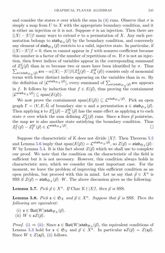
GRAPHICAL PLANAR ALGEBRAS 245
and consider the states σ over which the sum in (4) runs. Observe that σ issimply a map from U to X with the appropriate boundary condition, and itis either an injection or it is not. Suppose σ is an injection. Then there are(|X| − |U |)! many ways to extend σ to a permutation of X. Any such per-mutation belongs to stabSX
(~p) by the boundary condition, and converselyany element of stabSX
(~p) restricts to a valid, injective state. In particular, if(|X|−|U |)! = 0, then m cannot appear in f with nonzero coefficient becausethis number is a factor of the number of repetitions of m. If σ is not an injec-tion, then fewer indices of variables appear in the corresponding summandof ZL∆(~p) than in m because two or more have been identified by σ. Thus∑
s∈stabSX(~p) sm−α(|X|− |U |)!(ZL∆(~p)−ZW∆ (~p)) consists only of monomial
terms with fewer distinct indices appearing on the variables than in m. Bythe definition of [LstabSX
(~p)], every summand of∑
s∈stabSX(~p) sm appears
in f . It follows by induction that f ∈ E(~p), thus proving the containment[LstabSX
(~p)] ⊆ span(E(~p)).We now prove the containment span(E(~p)) ⊆ LstabSX
(~p). Pick an opengraph Γ = (V,E,~b) of boundary size n and a permutation s ∈ stabSX
(~p).Then applying s to ZL∆(~p)−ZW∆ (~p) has the same effect as applying s to eachstate σ over which the sum defining ZL∆(~p) runs. Since s fixes ~p pointwise,the map sσ is also another state satisfying the boundary condition. ThusZLΓ (~p)− ZWΓ (~p) ∈ LstabSX
(~p).
Suppose the characteristic of K does not divide |X|!. Then Theorem 5.5and Lemma 5.6 imply that span(E(~p)) = LstabSX
(~p), so Z(~p) = stabSX(~p) ·
W by Lemma 5.4. It is this fact about Z(~p) which we shall use to completeour proof. We note that the condition on the characteristic of the field issufficient but it is not necessary. However, this condition always holds incharacteristic zero, which we consider the most important case. For themoment, we leave the problem of improving this sufficient condition as anopen problem, but proceed with this in mind. Let us say that ~p ∈ Xn isSSS if Z(~p) = stabSX
(~p) ·W . The above discussion gives us the following:
Lemma 5.7. Pick ~p ∈ Xn. If Char K - |X|!, then ~p is SSS.
Lemma 5.8. Pick s ∈ SX and ~p ∈ Xn. Suppose that ~p is SSS. Then thefollowing are equivalent:
(i) s ∈ Aut(W )stabSX(~p).
(ii) W ∈ sZ(~p).
Proof. (i) ⇒ (ii): Since s ∈ Aut(W )stabSX(~p), the equivalent conditions of
Lemma 5.3 hold for s ∈ SX and ~p ∈ Xn. In particular sZ(~p) = Z(s~p).Since W ∈ Z(s~p), (ii) follows.

246 BRIAN CURTIN
(ii)⇒ (i): Since s−1W ∈ Z(~p), SSS implies that there exists t ∈ stabSX(~p)
such that s−1W = tW . Thus, stW = W , so st ∈ Aut(W ) by definition. Now(i) follows.
Lemma 5.9. Pick ~p, ~q ∈ Xn, and suppose that ~p and ~q are SSS. If ZW∆ (~p) =ZW∆ (~q) for all ∆ ∈ On, then ~p and ~q belong to the same Aut(W )-orbit ofXn.
Proof. By Lemma 5.2, there exists s ∈ SX with s~p = ~q. Now ZW∆ (~p) =ZW∆ (s~p) for all ∆ ∈ On, so sZ(~p) = Z(s~p) by Lemma 5.3. In particular, W ∈sZ(~p) sinceW ∈ Z(s~p). Now Lemma 5.8 implies that s ∈ Aut(W )stabSX
(~p).If s ∈ stabSX
(~p), then ~p = ~q. Otherwise, s 6∈ stabSX(~p), so there must be
an automorphism of W which maps ~p to ~q. In either case, ~p and ~q belongto the same Aut(W )-orbit of Xn.
Theorem 5.10. Let K denote a field, let X denote a finite, nonempty set,and pick W ∈MK(X). Suppose that Char K - |X|!. Then OW = FW .
Proof. Immediate from Lemmas 5.1, 5.7 and 5.9.
This completes our main results. We now give an example which showsthat OW need not equal FW if |X|! is divisible by the characteristic of K.
Example 5.11. Take as the ground field F2, the integers modulo 2. LetW denote the adjacency matrix of the complete bipartite graph K1,3 onvertex set X. Each partite set is an orbit of K1,3 under the action of itsautomorphism group, so dimF1(X,Aut(W )) = 2. However, dimOW
1 = 1since the symmetry of K1,3 implies that given an open graph ∆ = (V,E, b)of boundary size 1, ZW∆ (p) ≡ ZW∆ (q) (mod 2) for all vertices p, q of K1,3. Inparticular, OW
1 6= FW1 over F2. Similar arguments show that when W is the
adjacency matrix of a complete multipartite graph Kn1,n2,...,nm over a fieldK of characteristic k > 0, dimOW
1 is equal to the number of congruenceclasses modulo k appearing among n1, n2, . . . , nm while dimFW
1 is equalto the number of distinct numbers among n1, n2, . . . , nm.
The arguments used in this paper can be extended to planar subalgebrasof X generated by finitely many functions Ω = fi : Xki → K. Here theelements of the planar algebra PΩ are the functions defined from the par-tition function (1) starting from planar tangles all of whose internal disksare labeled with compatible elements of Ω. (See [15] for more on labeledplanar tangles.) The planar algebra OΩ can be defined using “open hyper-graphs” in a fashion similar to the definition of OW above. Then PΩ = OΩ
if and only if ΦΩ ∈ PΩ4 . Moreover, OΩ = F(Aut(Ω), X) as long as the
characteristic of the ground field does not divide the order of Aut(Ω), whereAut(Ω) = s ∈ SX | sfi = fi for all fi ∈ Ω.

GRAPHICAL PLANAR ALGEBRAS 247
References
[1] R.J. Baxter, Exactly Solved Models in Statistical Mechanics, Academic Press, London-New York, 1982, MR 86i:82002a, Zbl 0538.60093.
[2] N. Biggs, Interaction Models, London Mathematical Society Lecture Note Series, 30,Cambridge University Press, Cambridge-New York-Melbourne, 1977, MR 58 #32647,Zbl 0375.05039.
[3] D. Bisch and V.F.R. Jones, Singly generated planar algebras of small dimension, DukeMath. J., 101 (2000), 41-75, MR 2002f:46118.
[4] J.H. Conway, An enumeration of knots and links, and some of their algebraic proper-ties, Computational Problems in Abstract Algebra (Proc. Conf. Oxford, 1967), 1970,329-358, MR 41 #2661, Zbl 0202.54703.
[5] H. Ehrig, G. Engels, H.-J. Kreowski and G. Rozenberg, eds., Handbook of GraphGrammars and Computing by Graph Transformation. Vol. 2. Applications, Lan-guages and Tools, World Scientific Publishing Co., Inc., River Edge, NJ, 1999,MR 2001d:68012.
[6] H. Ehrig, H.-J. Kreowski, U. Montanari and G. Rozenberg, Handbook of GraphGrammars and Computing by Graph Transformation. Vol. 3. Concurrency, Paral-lelism, and Distribution, World Scientific Publishing Co., Inc., River Edge, NJ, 1999,MR 2001d:68013, Zbl 0951.68049.
[7] G. Hahn and C. Tardif, Graph homomorphisms: Structure and symmetry, in ‘GraphSymmetry (Montreal, PQ, 1996),’ 107-166, NATO Adv. Sci. Inst. Ser. C Math. Phys.Sci., 497, Kluwer Acad. Publ., Dordrecht, 1997, MR 99c:05091, Zbl 0880.05079.
[8] P. de la Harpe and V.F.R. Jones, Graph invariants related to statistical mechanicalmodels: Examples and problems, J. Combin. Theory Ser. B, 57(2) (1993), 207-227,MR 94c:05033, Zbl 0729.57003.
[9] P. Hell and J. Nesetril, On the complexity of H-coloring, J. Combin. Theory Ser. B,48 (1990), 92-110, MR 91m:68082, Zbl 0639.05023.
[10] , The existence problem for graph homomorphisms, in ‘Graph Theory in Mem-ory of G.A. Dirac (Sandbjerg, 1985),’ 255-265, Ann. Discrete Math., 41, North-Holland, Amsterdam-New York, 1989, MR 90b:05051, Zbl 0673.05033.
[11] G. James and M. Liebeck, Representations and Characters of Groups, Cam-bridge Mathematical Textbooks, Cambridge University Press, Cambridge, 1993,MR 94h:20007, Zbl 0792.20006.
[12] V.F.R. Jones, Hecke algebra representations of braid groups and link polynomials,Ann. of Math., 126 (1987), 335-388, MR 89c:46092, Zbl 0631.57005.
[13] , On knot invariants related to some statistical mechanical models, PacificJ. Math., 137 (1989), 311-224, MR 89m:57005, Zbl 0695.46029.
[14] , Subfactors and Knots, CBMS Regional Conference Series in Mathematics,80, Published for the Conference Board of the Mathematical Sciences, Washing-ton, DC; American Mathematical Society, Providence, RI, 1991, MR 93b:57008,Zbl 0743.46058.
[15] , Planar algebras, I, NZ J. Math, to appear.
[16] , The planar algebra of a bipartite graph, in ‘Knots in Hellas ’98 (Delphi)’,94-117, Ser. Knots Everything, 24, World Sci. Publishing, River Edge, NJ, 2000,CMP 1 865 703.

248 BRIAN CURTIN
[17] U. Montanari and F. Rossi, Graph rewriting, constraint solving and tiles for co-ordinating distributed systems, Alg. Categorical Structures, 7 (1999), 333-370,MR 2001b:68070, Zbl 0949.68083.
[18] E. Noether, Der Endlichkeitssatz der Invarianten endlicher Gruppen, Math. Ann., 77(1916), 89-92.
[19] , Der Endlichkeitssatz der Invarianten endlicher linearer Gruppen der charak-teristic p, Abh. Akad. Wiss. Gottingen, 1926, 28-35.
[20] G. Rozenberg, ed., Handbook of Graph Grammars and Computing by Graph Trans-formation. Vol. 1. Foundations, World Scientific Publishing Co., Inc., River Edge,NJ, 1997, MR 99b:68006, Zbl 0908.68095.
[21] L. Smith, Polynomial Invariants of Finite Groups, Research notes in mathematics,A.K. Peters, Ltd, Wellesley MA, 1995, MR 96f:13008, Zbl 0864.13002.
[22] B. Sturmfels, Algorithms in Invariant Theory, Springer-Verlag, Vienna, 1993,MR 94m:13004, Zbl 0802.13002.
[23] H.N.V. Temperley, Graph Theory and Applications, Ellis Horwood Ltd., Chichester;Halsted Press, New York, 1981, MR 83d:05001, Zbl 0481.05001.
[24] , Lattice models in discrete statistical mechanics, in ‘Applications of GraphTheory,’ R.J. Wilson and L.W. Beineke, Eds., Academic Press, London-New York,1979, Zbl 0444.05047.
Received February 5, 2001 and revised June 27, 2002. Research conducted while theauthor was an NSF mathematical sciences postdoctoral research fellow at UC-Berkeley.
Department of MathematicsUniversity of South Florida4202 E. Fowler Avenue, PHY114Tampa, FL 33620E-mail address: [email protected]

PACIFIC JOURNAL OF MATHEMATICSVol. 209, No. 2, 2003
COMPLETE CONTRACTIVITY OF MAPS ASSOCIATEDWITH THE ALUTHGE AND DUGGAL TRANSFORMS
Ciprian Foias, Il Bong Jung, Eungil Ko, and Carl Pearcy
For an arbitrary operator T on Hilbert space, we study themaps Φ : f(T ) → f(T ) and Φ : f(T ) → f(T ), where T and Tare the Aluthge and Duggal transforms of T , respectively, andf belongs to the algebra Hol(σ(T )). We show that both mapsare (contractive and) completely contractive algebra homo-morphisms. As applications we obtain that every spectral setfor T is also a spectral set for T and T , and also the inclusionW (f(T ))− ∪ W (f(T ))− ⊂ W (f(T ))− relating the numericalranges of f(T ), f(T ), and f(T ).
1. Introduction.
Let H be an arbitrary separable, complex Hilbert space whose dimensionsatisfies 2 ≤ dimH ≤ ℵ0, and denote by L(H) the algebra of all boundedlinear operators on H. If T ∈ L(H) we shall always write, without furthermention, T = UP to be the unique polar decomposition of T (so P = |T | =(T ∗T )
12 and U is the appropriate partial isometry satisfying kerU = kerT
and kerU∗ = kerT ∗). Also we write, as usual, σ(T ) for the spectrum ofsuch a T .
In this paper we consider the following two transforms of an arbitraryT = UP in L(H):
(a) the Aluthge transform T := P12UP
12 , which was first studied in [1]
and which has been studied extensively since, mostly in the context of p-hyponormal operators. In particular, some of the present authors studiedthe map T → T for an arbitrary T in L(H) in [4], [5] and [6].
We obtained in [4] various spectral identities and showed that if T is aquasiaffinity, then the invariant subspace lattice Lat(T ) is nontrivial if andonly if Lat(T ) is nontrivial, and the same is true of the hyperinvariant sub-space lattices HLat(T ) and HLat(T ). Furthermore, we showed that the mapT → T is (‖ ‖, ‖ ‖) continuous at every T in L(H) with closed range, andwe conjectured that for an arbitrary T in L(H), where H is finite dimen-sional, the sequence T (n) of Aluthge iterates of T , defined by T (0) = T
and T (n+1) = (T (n))˜ for n ∈ N, converges to a normal operator. Our studywas continued in [5], in which we showed that if T is an arbitrary operator
249

250 CIPRIAN FOIAS, IL BONG JUNG, EUNGIL KO, AND CARL PEARCY
in L(H) such that the spectral picture SP(T ) of T (or that of T ; cf. [9])contains no pseudoholes, then SP(T ) = SP(T ), and we derived connectionsbetween T and T as consequences of this equality (e.g., T is quasitriangularif and only if T is quasitriangular).
Moreover, in [6] we pursued the study of the sequence T (n) of Aluthgeiterates of an arbitrary T in L(H), and we established the validity of [4,Conjecture 1.11] in certain special cases. We also initiated a study of thebackward Aluthge iterates of an arbitrary T in L(H).
(b) The Duggal transform T := PU (named after Professor B. P. Duggal,who suggested its study to us), has been studied very little.
We will explore below various relations between T, T , and T by studyingmaps between the Riesz-Dunford algebras associated with these operators.It is well-known (and not difficult to see, cf. [4]) that
σ(T ) = σ(T ) = σ(T ), T ∈ L(H).
In what follows, when some T in L(H) is under consideration, we denoteby Hol(σ(T )) the algebra of all complex-valued functions which are analyticon some neighborhood of σ(T ), where linear combinations and products inHol(σ(T )) are defined (with varying domains) in the obvious way. Moreover,the (Riesz-Dunford) algebra AT ⊂ L(H) is defined as
AT = f(T ) : f ∈ Hol(σ(T )),
(where f(T ) is defined by the Riesz-Dunford functional calculus). As ourmain theorem (Th. 1.1) shows, it is possible to obtain useful informationabout T and T by studying maps between the algebras AT , A eT , and A bT .
Theorem 1.1. For every T in L(H), with T , T , and Hol (σ(T )) as definedabove:
a) The maps Φ : AT → AbT and Φ : AT → AeT defined by
Φ(f(T )) = f(T ), Φ(f(T )) = f(T ), f ∈ Hol (σ(T )),
are well-defined contractive algebra homomorphisms; in particular,
max‖f(T )‖, ‖f(T )‖ ≤ ‖f(T )‖, f ∈ Hol (σ(T )).(1)
b) More generally, the maps Φ and Φ in a) are completely contractive,meaning that for every n ∈ N and every n×n matrix (fij) with entriesfrom Hol (σ(T )),
max‖(fij(T ))‖, ‖(fij(T ))‖ ≤ ‖(fij(T ))‖.
c) Every spectral set [M -spectral set (for fixed M > 1)] for T is also aspectral set [respectively, M -spectral set ] for both T and T .
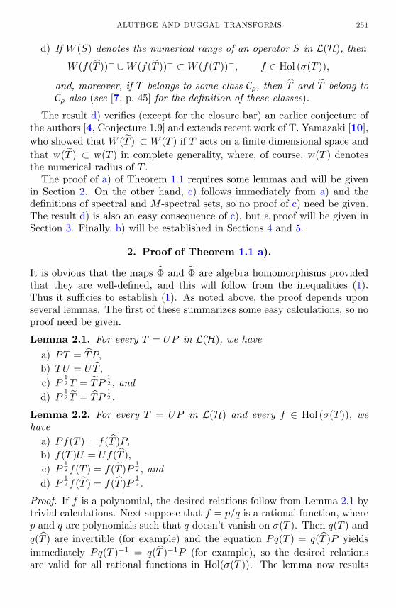
ALUTHGE AND DUGGAL TRANSFORMS 251
d) If W (S) denotes the numerical range of an operator S in L(H), then
W (f(T ))− ∪W (f(T ))− ⊂W (f(T ))−, f ∈ Hol (σ(T )),
and, moreover, if T belongs to some class Cρ, then T and T belong toCρ also (see [7, p. 45] for the definition of these classes).
The result d) verifies (except for the closure bar) an earlier conjecture ofthe authors [4, Conjecture 1.9] and extends recent work of T. Yamazaki [10],who showed that W (T ) ⊂W (T ) if T acts on a finite dimensional space andthat w(T ) ⊂ w(T ) in complete generality, where, of course, w(T ) denotesthe numerical radius of T .
The proof of a) of Theorem 1.1 requires some lemmas and will be givenin Section 2. On the other hand, c) follows immediately from a) and thedefinitions of spectral and M -spectral sets, so no proof of c) need be given.The result d) is also an easy consequence of c), but a proof will be given inSection 3. Finally, b) will be established in Sections 4 and 5.
2. Proof of Theorem 1.1 a).
It is obvious that the maps Φ and Φ are algebra homomorphisms providedthat they are well-defined, and this will follow from the inequalities (1).Thus it sufficies to establish (1). As noted above, the proof depends uponseveral lemmas. The first of these summarizes some easy calculations, so noproof need be given.
Lemma 2.1. For every T = UP in L(H), we have
a) PT = TP,
b) TU = UT ,
c) P12T = TP
12 , and
d) P12 T = TP
12 .
Lemma 2.2. For every T = UP in L(H) and every f ∈ Hol (σ(T )), wehave
a) Pf(T ) = f(T )P,b) f(T )U = Uf(T ),c) P
12 f(T ) = f(T )P
12 , and
d) P12 f(T ) = f(T )P
12 .
Proof. If f is a polynomial, the desired relations follow from Lemma 2.1 bytrivial calculations. Next suppose that f = p/q is a rational function, wherep and q are polynomials such that q doesn’t vanish on σ(T ). Then q(T ) andq(T ) are invertible (for example) and the equation Pq(T ) = q(T )P yieldsimmediately Pq(T )−1 = q(T )−1P (for example), so the desired relationsare valid for all rational functions in Hol(σ(T )). The lemma now results

252 CIPRIAN FOIAS, IL BONG JUNG, EUNGIL KO, AND CARL PEARCY
easily from Runge’s theorem and the well-known continuity properties ofthe Riesz-Dunford functional calculus (cf., e.g., [2, Prop. 17.26]).
Lemma 2.3. For every T = UP in L(H) and every f ∈ Hol (σ(T )), f(T )is the (orthogonal ) direct sum
f(T ) = EU∗f(T )UE|(kerT )⊥ ⊕ f(0)1kerT ,(2)
where E is the (orthogonal) projection U∗U on (kerT )⊥, and, consequently,
‖f(T )‖ ≤ ‖f(T )‖.(3)
Proof. If T has trivial kernel, then U is an isometry, and thus E = 1Hand f(T ) = U∗f(T )U , so (2) and (3) are satisfied. Thus we may supposethat 0 ∈ σ(T ), and hence f is analytic at z = 0 and f(0) ∈ σ(f(T )). Aneasy calculation shows that ET = TE = T , and thus (by writing f(z) =f(0) + zg(z), where g ∈ Hol(σ(T ))) that f(T )E = Ef(T ). Hence
f(T ) = Ef(T )E|(kerT )⊥ ⊕ f(0)1kerT
= EU∗f(T )UE|(kerT )⊥ ⊕ f(0)1kerT ,
from b) of Lemma 2.2, and thus
‖f(T )‖ ≤ max‖f(T )‖, |f(0)| = ‖f(T )‖.
Lemma 2.4. For every T = UP in L(H) such that P has trivial ker-nel (which implies, of course, that U is an isometry) and for every f ∈Hol (σ(T )), ‖f(T )‖ ≤ ‖f(T )‖.
Proof. Suppose first that P is invertible. We use the fact from [3] that ifX ∈ L(H) and A and B are positive semidefinite operators in L(H), then
‖A12XB
12 ‖ ≤ ‖AXB‖
12 ‖X‖
12 .(4)
We know from c) of Lemma 2.2 that
f(T ) = P12 f(T )P−
12 ,
so applying (4) with A = P and B = P−1 we obtain
‖f(T )‖ = ‖P12 f(T )P−
12 ‖ ≤ ‖Pf(T )P−1‖
12 ‖f(T )‖
12 .(5)
Moreover, we know from a) of Lemma 2.2 that
Pf(T )P−1 = f(T ),
and thus (5) becomes
‖f(T )‖ ≤ ‖f(T )‖12 ‖f(T )‖
12 ≤ ‖f(T )‖,
by Lemma 2.3, and the case in which P is invertible is done.

ALUTHGE AND DUGGAL TRANSFORMS 253
Now let P be an arbitrary quasiaffinity. Define the sequence Qn ofpositive invertible operators by Qn = P + (1/n)1H, and set An = UQn(polar decomposition of An). Then An = (Qn)1/2U(Qn)1/2, and since ‖Qn−P‖ → 0 and ‖(Qn)1/2 − P 1/2‖ → 0, we obtain that ‖An − T‖ → 0 and‖An − T‖ → 0. By what was proved above, we have ‖f(An)‖ ≤ ‖f(An)‖for all n sufficiently large that f(An) is defined. The result follows from thefacts that ‖f(An)− f(T )‖ → 0 and ‖f(An)− f(T )‖ → 0 (cf., for example,[2, Prop. 17.26]).
Lemma 2.5. For every T = UP in L(H) such that
dim(kerU∗) ≥ dim(kerU) > 0
and for every f ∈ Hol (σ(T )), ‖f(T )‖ ≤ ‖f(T )‖.
Proof. Choose a partial isometry V such that the initial space of V is kerUand the range of V is a subspace of kerU∗. Define An = T + (1/n)V forn ∈ N, and note that each |An| is a quasiaffinity and that ‖An − T‖ → 0.Since the polar decomposition of An is (U +V )|An| where |An| is the directsum P |(kerT )⊥ ⊕ (1/n)1kerT , it follows easily that ‖An − T‖ → 0. FromLemma 2.4 we know that ‖f(An)‖ ≤ ‖f(An)‖ and the result now follows asbefore from, e.g., [2, Prop. 17.26].
To complete the proof of a) of Theorem 1.1, it suffices, in view of Lem-ma 2.5, to deal with the case in which T = UP and U satisfies dim(kerU∗) <dim(kerU). Moreover, if kerU∗ is nontrivial, by choosing a partial isometryW whose range is kerU∗ and whose initial space is a subspace of kerU , andconsidering the sequence T + (1/n)W as in Lemma 2.5, we can reducewhat is to be shown to the case in which U is a nonunitary coisometry.
Lemma 2.6. For every T = UP in L(H) such that U is a nonunitarycoisometry and for every f ∈ Hol (σ(T )),
‖f(T )‖ ≤ ‖f(T )‖ ≤ ‖f(T )‖.
Proof. Let U∗ := z : z ∈ U, and let f be the analytic function on U∗defined, as usual, by f(z) := f(z), z ∈ U∗. Recall that in this situation,σ(T ∗) ⊂ U∗ and f(T )∗ = f(T ∗), so ‖f(T ∗)‖ = ‖f(T )‖. Note that T = PU ,and thus that (T )∗ = U∗P with U∗ an isometry. Define, for n ∈ N,
Sn = U∗(P + (1/n)1H).(6)
Since P +(1/n)1H is invertible, (6) gives the polar decomposition of Sn, andhence
Sn = (P + (1/n)1H)12U∗(P + (1/n)1H)
12 , n ∈ N.(7)

254 CIPRIAN FOIAS, IL BONG JUNG, EUNGIL KO, AND CARL PEARCY
It follows easily that ‖Sn − (T )∗‖ → 0 and that ‖Sn − (T )∗‖ → 0. Thus wehave
‖f(T )‖ = ‖f((T )∗)‖ = limn‖f(Sn)‖,
and
‖f(T )‖ = ‖f((T )∗)‖ = limn‖f(Sn)‖
(again by, e.g., [2, Prop. 17.26]). But Lemma 2.4 applies to each Sn, andthus
‖f(Sn)‖ ≤ ‖f(Sn)‖, n ∈ N.
Thus ‖f(T )‖ ≤ ‖f(T )‖ and the other inequality follows from Lemma 2.3.This completes the proof of Theorem 1.1 a).
3. Proof of Theorem 1.1 d).
In view of Theorem 1.1 c), which follows immediately from Theorem 1.1 a)as noted above, the first statement in d) follows trivially from the followingknown fact, and the other statements are immediate from Remarks 1, 2 and3 on pp. 48 and 49 of [7]:
Proposition 3.1. For every T ∈ L(H), W (T )− is the intersection of allclosed half-planes H containing W (T ) such that H is a spectral set for T.
Proof. Since W (T )− is convex, and is thus the intersection of all closed half-planes containing W (T ), it suffices to show that if H is any closed halfplanecontaining W (T ), then H is a spectral set for T . By a harmless rota-tion and translation, we may suppose that H is the closed right-halfplanez : Re z ≥ 0. Thus, writing T = K + iL, with K and L Hermitian, we seethat K is positive semidefinite, and therefore that the Cayley transform ofT,
c(T ) = (T + 1H)−1(T − 1H),
is a contraction (cf., e.g., [7, p. 167]). Hence, by von Neuman’s inequality,the closed unit disc D in C is a spectral set for c(T ), and thus, by takinginverse Cayley transforms, we obtain that H is a spectral set for T , asdesired.
4. Complete contractivity of Φ.
In this section we prove the following theorem, which establishes a part ofTheorem 1.1 b):
Theorem 4.1. For every T in L(H), the map Φ : AT → AbT defined inSection 1 is completely contractive.

ALUTHGE AND DUGGAL TRANSFORMS 255
Recall that this means, by definition, that for every n ∈ N and for everyn× n matrix (fij), where each fij ∈ Hol(σ(T )), the inequality
‖(fij(T ))‖ ≤ ‖(fij(T ))‖(8)
is satisfied. (Here of course, the n × n operator matrices in (8) act on theHilbert space H(n), the direct sum of n copies of H, and the norm indicatedis the operator norm on L(H(n)).)
Proof of Theorem 4.1. Let T ∈ L(H), let n ∈ N, and let (fij) be an arbitraryn × n matrix with entries from Hol(σ(T )). Then, with the notation as inLemma 2.3, it is immediate from (2) that we have the matricial identity
(fij(T )) = (EU∗fij(T )UE|(kerT )⊥)⊕ (fij(0)1kerT ),(9)
where, of course, the first [second] matrix on the right acts on the space(kerT )⊥(n) [respectively, kerT(n)]. As in the proof of Lemma 2.3, if Thas trivial kernel, then E = 1H and U is an isometry. Since it is obviousthat the inequality
‖(U∗fij(T )U)‖ ≤ ‖(fij(T ))‖(10)
holds (the matrix on the left is the product of two diagonal matrices ofnorm at most one and the matrix on the right), it suffices to treat the casein which kerT 6= (0). Moreover, from (9), one sees easily that it is enoughto show that
‖(fij(0)1kerT )‖ ≤ ‖(fij(T ))‖.(11)
Since fij(0) ∈ σ(fij(T )), fij is analytic at z = 0 for i, j = 1, . . . , n. Uponwriting
fij(z)− fij(0) = gij(z)z, z ∈ domain fij ,
we see that gij(z) ∈ Hol(σ(T )) for i, j = 1, . . . , n, and hence we get thematricial identity
(fij(T )− fij(0)1H) = (gij(T )T ) = (gij(T )) Diag (T, . . . , T ).(12)
Observe next that the matrix (fij(0)1kerT ) has the same norm as thematrix M = (fij(0)) acting on Cn. Moreover, there exists a unit vectorw = (ξ1, . . . , ξn)t in Cn such that ‖Mw‖ = ‖M‖. Now let x be a unit vectorin ker(T ) and note that if s is the unit vector
s = (ξ1x, . . . , ξnx)t ∈ H(n),
then, from (12), we have (fij(T ))s = (fij(0)1H)s. Write Mw = (γ1, . . . , γn)t,and observe that
‖M‖ = ‖Mw‖ =∥∥(γ1, . . . , γn)t
∥∥ =∥∥(γ1x, . . . , γnx)t
∥∥= ‖(fij(0)1H)s‖ = ‖(fij(T ))s‖ ≤ ‖(fij(T ))‖ ,
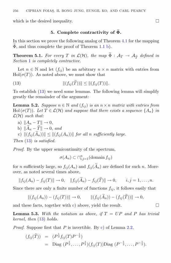
256 CIPRIAN FOIAS, IL BONG JUNG, EUNGIL KO, AND CARL PEARCY
which is the desired inequality.
5. Complete contractivity of Φ.
In this section we prove the following analog of Theorem 4.1 for the mappingΦ, and thus complete the proof of Theorem 1.1 b).
Theorem 5.1. For every T in L(H), the map Φ : AT → AeT defined inSection 1 is completely contractive.
Let n ∈ N and let (fij) be an arbitrary n × n matrix with entries fromHol(σ(T )). As noted above, we must show that
‖(fij(T ))‖ ≤ ‖(fij(T ))‖.(13)
To establish (13) we need some lemmas. The following lemma will simplifygreatly the remainder of the argument:
Lemma 5.2. Suppose n ∈ N and (fij) is an n×n matrix with entries fromHol (σ(T )). Let T ∈ L(H) and suppose that there exists a sequence An inL(H) such that:
a) ‖An − T‖ → 0,b) ‖An − T‖ → 0, andc) ‖(fij(An))‖ ≤ ‖(fij(An))‖ for all n sufficiently large.
Then (13) is satisfied.
Proof. By the upper semicontinuity of the spectrum,
σ(An) ⊂ ∩ni,j=1(domain fij)
for n sufficiently large, so fij(An) and fij(An) are defined for such n. More-over, as noted several times above,
‖fij(An)− fij(T )‖ → 0, ‖fij(An)− fij(T )‖ → 0, i, j = 1, . . . , n.
Since there are only a finite number of functions fij , it follows easily that
‖(fij(An))− (fij(T ))‖ → 0, ‖(fij(An))− (fij(T ))‖ → 0,
and these facts, together with c) above, yield the result.
Lemma 5.3. With the notation as above, if T = UP and P has trivialkernel, then (13) holds.
Proof. Suppose first that P is invertible. By c) of Lemma 2.2,
(fij(T )) = (P12 fij(T )P−
12 )
= Diag (P12 , . . . , P
12 )(fij(T ))Diag (P−
12 , . . . , P−
12 ).

ALUTHGE AND DUGGAL TRANSFORMS 257
Thus, utilizing (4), Lemma 2.2 a), and Theorem 4.1, we obtain
‖(fij(T ))‖ ≤ ‖(Pfij(T )P−1)‖12 ‖(fij(T ))‖
12
= ‖(fij(T ))‖12 ‖(fij(T ))‖
12
≤ ‖(fij(T ))‖,
as desired. Now let P be an arbitrary quasiaffinity, and let the sequencesQn and An be as defined in the proof of Lemma 2.4, so we have a) andb) of Lemma 5.2 satisfied. Since each |An| is invertible by construction, bywhat was just shown,
‖(fij(An))‖ ≤ ‖(fij(An))‖,
so c) of Lemma 5.2 is satisfied and the result follows from that lemma.
Lemma 5.4. Let n ∈ N, let (fij) be any n × n matrix with entries fromHol (σ(T )) and suppose T = UP is any operator in L(H) such that
dim(kerU∗) ≥ dim(kerU) > 0.
Then (13) is satisfied.
Proof. Let the sequence An∞n=1 be as defined in Lemma 2.5, and observethat from the proof of that lemma, we know that a) and b) of Lemma 5.2are satisfied. Moreover, since each |An| is a quasiaffinity, Lemma 5.3 yieldsthat c) of Lemma 5.2 is satisfied, and the result follows from Lemma 5.2.
In view of the discussion preceding Lemma 2.6, the proof of Theorem 5.1(and thus the proof of Theorem 1.1 b) is completed by the following:
Lemma 5.5. For every T = UP in L(H) such that U is a nonunitarycoisometry, for every n ∈ N, and for every n × n matrix (fij) with entriesfrom Hol (σ(T )), (13) is satisfied.
Proof. Let the sequence Sn∞n=1 be as defined in the proof of Lemma 2.6,and observe from that proof that ‖Sn − (T )∗‖ → 0 and ‖Sn − (T )∗‖ → 0.Moreover, since |Sn| is an isometry for each n, Lemma 5.4 applies to givethat
‖(fij(Sn))‖ ≤ ‖(fij(Sn))‖,
so that a), b) and c) of Lemma 5.2 are satisfied (with Sn → An (i.e., Snreplaces An), T ∗ → T, T ∗ → T , and fij → fij), so
‖(fij(T ∗))‖ ≤ ‖(fij(T ∗))‖.(14)
Upon taking adjoints in (14) and using Theorem 4.1, the result follows.

258 CIPRIAN FOIAS, IL BONG JUNG, EUNGIL KO, AND CARL PEARCY
Of course, one reason for establishing that the maps Φ and Φ are com-pletely contractive is that the extension theorems of Arveson and Stinespringcan be applied to obtain the structure of such maps (cf., e.g., [8]), and thuswe get the following:
Theorem 5.6. Let T be an arbitrary operator in L(H), and let Φ and Φ bethe maps defined in Theorem 1.1. Then there exist Hilbert spaces K = KTand K = KT containing H, and C∗-homomorphisms Ψ : C∗(T ) → L(K)and Ψ : C∗(T ) → L(K) (where C∗(T ) is the smallest unital C∗-algebracontaining AT ) such that for every f in Hol (σ(T )),
Φ(f(T )) = PHΨ(f(T ))|Hand
Φ(f(T )) = P(2)H Ψ(f(T ))|H,
where P (1)H and P (2)
H are the orthogonal projections of K and K, respectively,onto H.
The implications of Theorem 5.6 for the Aluthge and Duggal transformswill be the subject of a forthcoming paper by the authors.
Acknowledgement. The second and third authors were supported byKOSEF Research Project No. R01-2000-00003. The fourth author acknowl-edges the support of the National Science Foundation.
References
[1] A. Aluthge, On p-hyponormal operators for 0 < p < 1, Integral Equations OperatorTheory, 13 (1990), 307-315, MR 91a:47025, Zbl 0718.47015.
[2] A. Brown and C. Pearcy, Introduction to Operator Theory I, Springer Verlag, NewYork, 1977, MR 58 #23463, Zbl 0371.47001.
[3] E. Heinz, Beitrae zur Storungstheorie der Spektralzerlegung, Math. Ann., 123 (1951),415-438, MR 13,471f, Zbl 0043.32603.
[4] I. Jung, E. Ko and C. Pearcy, Aluthge transforms of operators, Integral EquationsOperator Theory, 37 (2000), 437-448, MR 2001i:47035.
[5] , Spectral pictures of Aluthge transforms of operators, Integral Equations Op-erator Theory, 40 (2001), 52-60, MR 2002b:47007.
[6] , The iterated Aluthge transform of an operator, Integral Equations OperatorTheory, to appear.
[7] B. Sz.-Nagy and C. Foias, Harmonic Analysis of Operators on Hilbert Space, North-Holland, Amsterdam, 1970, MR 43 #947, Zbl 0201.45003.
[8] V. Paulsen, Completely Bounded Maps and Dilations, Longman Sci. & Tech. PittmanResearch Note 146, 1986, MR 88h:46111, Zbl 0614.47006.

ALUTHGE AND DUGGAL TRANSFORMS 259
[9] C. Pearcy, Some Recent Developments in Operator Theory, C.B.M.S. Regional Confer-ence Series in Mathematics, 36, Amer. Math. Soc., Providence, 1978, MR 58 #7120,Zbl 0444.47001.
[10] T. Yamazaki, On numerical range of the Aluthge transformation, Linear Algebra andApplications, 341 (2002), 111-117, MR 2003a:47012.
Received April 4, 2002.
Department of MathematicsTexas A&M UniversityCollege Station, TX 77843E-mail address: [email protected]
Department of MathematicsKyungpook National UniversityTaegu 702-701KoreaE-mail address: [email protected]
Department of MathematicsEwha Women’s UniversitySeoul 120-750KoreaE-mail address: [email protected]
Department of MathematicsTexas A&M UniversityCollege Station, TX 77843E-mail address: [email protected]
PACIFIC JOURNAL OF MATHEMATICSVol. 209, No. 2, 2003
SOMMES DE MODULES DE SOMMESD’EXPONENTIELLES
Etienne Fouvry and Philippe Michel
Let Kl(a, b; n) be the usual Kloosterman sum modulo n,with coefficients a and b. We give upper and lower boundsfor the sum
∑n≤x |Kl(1, 1; n)|/
√n, and for related sums, by
using large sieve techniques and Deligne-Katz theory of expo-nential sums. Extensions to more general exponential sumsof dimension one are also given.
1. Introduction.
Soient a et b des entiers et n un entier ≥ 1. On rappelle que la sommede Kloosterman Kl(a, b;n), de denominateur n et de coefficients a et b, estdefinie par
Kl(a, b;n) =∑
(m,n)=1
exp(
2πiam+ bm
n
).
Systematiquement, le symbole m dans la fraction mn designe l’inverse mul-
tiplicatif de m modulo n, ω(n) est le nombre de facteurs premiers distinctsde l’entier n, et on reserve la lettre p aux nombres premiers. Les sommesde Kloosterman jouent un role crucial dans l’actuelle theorie analytique desnombres, au confluent de la geometrie algebrique et de la theorie des formesmodulaires. Rappelons que ce sont des nombres reels non nuls qui verifient,entre autres, les proprietes suivantes:
– Multiplicativite croisee: Pour (n1, n2) = 1, on a la relation
Kl(a, b;n1n2) = Kl(a, bn22;n1)Kl(a, bn1
2;n2).
– Majoration individuelle:
|Kl(a, b;n)| ≤ (a, b, n)12 2ω(n)n
12 ,(1.1)
consequence de la multiplicativite croisee, de la demonstration parWeil, de l’hypothese de Riemann pour les courbes sur les corps finis(qui donne (1.1) lorsque n = p) et de l’etude, due a divers auteurs, dessommes de Kloosterman de denominateur pk (k ≥ 2).
261

262 E. FOUVRY AND P. MICHEL
L’objet de cet article est de s’interesser, lorsque a et b sont fixes (disonsa = b = 1, pour fixer les idees), a l’optimalite de l’inegalite (1.1), lorsque nparcourt l’ensemble des entiers. Dans ce but on introduit les quantites
A∗(x) =∑n≤x
∣∣∣∣Kl(1, 1;n)2ω(n)
√n
∣∣∣∣ ,et
A(x) =∑n≤x
∣∣∣∣Kl(1, 1;n)√n
∣∣∣∣ ,qui verifient donc les inegalites triviales
A∗(x) ≤ x (x ≥ 1),(1.2)
et
A(x) ≤∑n≤x
2ω(n) ≤(
6π2
+ o(1))x log x (x −→∞).(1.3)
Les parties droites des inegalites (1.2) et (1.3) peuvent etre ameliorees d’uneconstante multiplicative, en injectant des majorations plus precises que (1.1)dans le cas ou n = pk (k ≥ 2), mais nous sommes concernes par des gainsplus substantiels, puisque nous montrerons les encadrements:
Theoreme 1.1. Il existe une constante absolue c∗1 et, pour tout k, une con-stante c∗0(k) > 0, telles que, pour x ≥ 3, on ait les inegalites
c∗0(k)x
log x(log log x)k ≤ A∗(x) ≤ c∗1 x
(log log x
log x
)1− 43π
.(1.4)
Theoreme 1.2. Il existe une constante absolue c1 et, pour tout k, une con-stante c0(k) > 0, telles que, pour x ≥ 3, on ait les inegalites
c0(k)x
log x(log log x)k ≤ A(x) ≤ c1x(log log x)
(log log x
log x
)1− 83π
.(1.5)
Ainsi, par rapport aux majorations triviales (1.2) et (1.3), on gagne re-spectivement (log x)−0,575587... et (log x)−1,151174.... A notre connaissance,la premiere majoration non triviale de A∗(x) ou de A(x) est due a Hooley([Ho] Theorem 3), ou il montre, pour u et v entiers la relation∑
n≤xKl(u, v;n) = O
x 32
∑d|v
d−12
(log x)√
2−1(log log x)c2
,(1.6)
ou c2 est une certaine constante. La preuve par Hooley de (1.6) donne enfait une majoration de
∑n≤x |Kl(u, v;n)|, qui conduit donc, dans notre cas,
a
A(x) ≤ c3x(log x)√
2−1(log log x)c2 ,(1.7)

SOMMES DE MODULES DE SOMMES D’EXPONENTIELLES 263
pour un certain c3 > 0, c’est-a-dire un gain de (log x)−0,585786..., par rapporta la majoration triviale (1.3).
La minoration (1.4) de A∗(x) ameliore notablement celle en
A(x) ≥ c4x/ log2 x,(1.8)
consequence directe de ([Mi1] Theoreme 1) ou il est montre, que pour x −→∞, on a
] (p1, p2) ;x < p1, p2 < 2x, |Kl(1, 1; p1p2)| ≥ 0, 64√p1p2
x2
log2 x.
Autant on devine une difference de comportement a l’infini des quantitesA∗(x) et A(x), dans les majorations (1.4) et (1.5), autant notre preuve nepermet guere de differencier les minorations de ces fonctions, si ce n’estqu’au §4, nous obtiendrons les constantes c0(k) = 2k+3c∗0(k). Rappelonsque l’on sait, grace a la theorie des formes modulaires, qu’il y a d’enormescompensations entre les signes des sommes de Kloosterman, puisqu’on apour tout ε > 0, la majoration ([Ku] et [D-I])∑
n≤x
Kl(1, 1;n)√n
= Oε
(x
23+ε),(1.9)
qu’il convient de comparer avec (1.3), alors que la conjecture de Linnik-Selberg predit meme une majoration en Oε(x
12+ε). Enfin, on ne sait pas si
la majoration (1.9) continue d’etre vraie si on insere au denominateur de lapartie gauche, le facteur arithmetique 2ω(n).
Ainsi le Theoreme 1.2 repond de facon plus precise que (1.7) et (1.8), ala question de l’origine des compensations dans (1.9): de facon succincte,on peut dire que le fait que les modules |Kl(1, 1;n)| (n ≤ x) soient petits enmoyenne ne fait gagner, par rapport a la majoration triviale∣∣∣∣∣∣
∑n≤x
Kl(1, 1;n)√n
∣∣∣∣∣∣ ≤ A(x) = O(x log x)
qu’un certain facteur X, verifiant log−2 x X (log x)−1,151174. Enconclusion, on peut affirmer que dans (1.9), la plus grande partie des com-pensations provient des changements de signe des sommes de Kloosterman.
En fait, comme nous le fit remarquer R. de la Breteche, on peut, dans lesminorations (1.4) et (1.5), donner explicitement les fonctions c∗0(k) et c0(k),puis prendre k comme fonction de x. Nous donnerons, au paragraphe 5, desindications menant au:
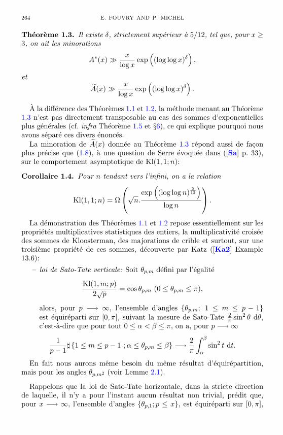
264 E. FOUVRY AND P. MICHEL
Theoreme 1.3. Il existe δ, strictement superieur a 5/12, tel que, pour x ≥3, on ait les minorations
A∗(x) x
log xexp
((log log x)δ
),
et
A(x) x
log xexp
((log log x)δ
).
A la difference des Theoremes 1.1 et 1.2, la methode menant au Theoreme1.3 n’est pas directement transposable au cas des sommes d’exponentiellesplus generales (cf. infra Theoreme 1.5 et §6), ce qui explique pourquoi nousavons separe ces divers enonces.
La minoration de A(x) donnee au Theoreme 1.3 repond aussi de faconplus precise que (1.8), a une question de Serre evoquee dans ([Sa] p. 33),sur le comportement asymptotique de Kl(1, 1;n):
Corollaire 1.4. Pour n tendant vers l’infini, on a la relation
Kl(1, 1;n) = Ω
√n.exp((log log n)
512
)log n
.
La demonstration des Theoremes 1.1 et 1.2 repose essentiellement sur lesproprietes multiplicatives statistiques des entiers, la multiplicativite croiseedes sommes de Kloosterman, des majorations de crible et surtout, sur unetroisieme propriete de ces sommes, decouverte par Katz ([Ka2] Example13.6):
– loi de Sato-Tate verticale: Soit θp,m defini par l’egalite
Kl(1,m; p)2√p
= cos θp,m (0 ≤ θp,m ≤ π),
alors, pour p −→ ∞, l’ensemble d’angles θp,m; 1 ≤ m ≤ p − 1est equireparti sur [0, π], suivant la mesure de Sato-Tate 2
π sin2 θ dθ,c’est-a-dire que pour tout 0 ≤ α < β ≤ π, on a, pour p −→∞
1p− 1
] 1 ≤ m ≤ p− 1 ;α ≤ θp,m ≤ β −→ 2π
∫ β
αsin2 t dt.
En fait nous aurons meme besoin du meme resultat d’equirepartition,mais pour les angles θp,m2 (voir Lemme 2.1).
Rappelons que la loi de Sato-Tate horizontale, dans la stricte directionde laquelle, il n’y a pour l’instant aucun resultat non trivial, predit que,pour x −→ ∞, l’ensemble d’angles θp,1; p ≤ x, est equireparti sur [0, π],

SOMMES DE MODULES DE SOMMES D’EXPONENTIELLES 265
suivant la mesure de Sato-Tate ([Ka1] Conj. 1.2.5). L’exactitude de cetteconjecture entraınerait, pour x −→∞, la relation∑
p≤x
∣∣∣∣Kl(1, 1; p)2√p
∣∣∣∣ ∼ 43π
· x
log x.
La recherche d’un equivalent asymptotique des sommes A∗(x) et A(x) paraıtainsi comme un probleme tres ardu, malgre l’encadrement etroit que four-nissent, pour chacune de ces sommes, les Theoremes 1.1, 1.2 et 1.3.
On peut etendre les resultats precedents a des sommes de la forme∑n≤x
∣∣∣∣Kl(1, 1;n)2ω(n)
√n
∣∣∣∣α ,ou ∑
n≤x
∣∣∣∣Kl(1, 1;n)√n
∣∣∣∣α ,avec α reel positif fixe, mais il est beaucoup plus interessant d’etudier lessommes trigonometriques plus generales
Sf (m;n) =∑
x (mod n)f(x) 6=∞
exp(
2πimf(x)n
)=
∑x (mod n)(Q(x),n)=1
exp
(2πi
mP (x)Q(x)n
),
pour:– n ≥ 1, m ∈ Z,– f = P
Q fraction rationnelle, quotient de deux polynomes P et Q, deZ[X], premiers entre eux, a coefficients premiers entre eux.
Les sommes Sf (m;n) verifient elles-aussi la multiplicativite croisee
Sf (m;n1n2) = Sf (mn1;n2)Sf (mn2;n1), pour (n1, n2) = 1,
et une majoration due a Weil (cf. [D] Formule (3.5.2) p. 191):
|Sf (m; p)| ≤ kf√p (p 6 |m),
ou kf etant un entier parfaitement defini en termes de la geometrie de lafraction f , c’est-a-dire
kf = maxdegP, degQ+ ] racines distinctes de Q − 1.
Le cas des Sf (m; pa), (a ≥ 2) mene a des situations delicates a traiteren toute generalite, nous preferons les eviter en ne considerant que des nsans facteur carre. Apres ces diverses considerations, nous etudions, pourx −→∞, les sommes
A∗f (x) :=∑n≤x
µ2(n)
∣∣∣∣∣∣Sf (1; n)
kω(n)f
√n
∣∣∣∣∣∣ ,
266 E. FOUVRY AND P. MICHEL
et
Af (x) :=∑n≤x
µ2(n)∣∣∣∣Sf (1; n)√
n
∣∣∣∣ ,dont des majorations triviales sont respectivement O(x) et O(x logkf−1 x).Katz ([Ka3] 7.9, 7.10, 7.11; voir aussi le debut du §5) a prouve aussi une loide Sato-Tate verticale pour la plupart des sommes Sf . Ainsi, si on pose
|Sf (m; p)|kf√p
= cos θf,p,m(0 ≤ θf,p,m ≤ π
2
),
Katz a montre que, pourvu que kf ≥ 2 et pourvu que f verifie des hypothesestres generales concernant essentiellement la nature et la disposition des zerosde f ′, l’ensemble des angles θf,p,m ; 1 ≤ m ≤ p−1 est equireparti sur [0, π2 ],lorsque p −→∞, suivant une certaine mesure que nous decrivons ci-dessouset que, par un certain abus de langage, nous appellerons aussi mesure deSato-Tate. De facon plus precise, si f est une fraction rationnelle commeci-dessus, on note Zf ′ l’ensemble des zeros de f ′ dans P1(C) et on poseCf = f(Zf ′). On designe par H.1, H.2, H.3 et H.3′ les hypotheses suivantes:
H.1: Les zeros de f ′ sont simples, (autrement dit ]Zf ′ = kf ).H.2: f separe les zeros de f ′ (autrement dit, pour z et z′ ∈ Zf ′, on a
l’implication f(z) = f(z′) ⇒ z = z′).H.3: On a l’implication
s1, s2, s3, s4 ∈ Cfet
s1 − s2 = s3 − s4
⇒
s1 = s2 et s3 = s4ou
s1 = s3 et s2 = s4.
H.3′: f est impaire et on a l’implication
s1, s2, s3, s4 ∈ Cfet
s1 − s2 = s3 − s4
⇒
s1 = s2 et s3 = s4
ous1 = s3 et s2 = s4
ous1 = −s4 et s2 = −s3.
On designe par
H l’ensemble des conditions H.1, H.2 et H.3
et par
H′ l’ensemble des conditions H.1, H.2 et H.3′.
Si la fraction rationnelle f verifie H, on pose
Gf = SUkf(C),
SOMMES DE MODULES DE SOMMES D’EXPONENTIELLES 267
et si f verifie H′, on pose
Gf = USpkf(C).
Si G designe l’un des groupes compacts SUk(C) ou USpk(C), on note µHaarG ,
la mesure de Haar sur le groupe G et µG l’image directe de µHaarG dans [0, π2 ],
par l’applicationG −→ [0, π2 ]
A 7−→ Arc cos(|trA|k
).
Avec ces conventions, une des consequences des travaux de Katz est que, sila fraction rationnelle f avec kf ≥ 2, verifie H ou H′, l’ensemble des anglesθf,p,m ; 1 ≤ m ≤ p− 1 est equireparti sur [0, π2 ], lorsque p −→ ∞, suivantla mesure µGf
.Au paragraphe §6, nous demontrerons:
Theoreme 1.5. Soit f une fraction rationnelle comme auparavant, aveckf ≥ 2, verifiant les conditions H ou H′. Il existe des constantes, c∗6 et c6et, pour tout k, des constantes c∗5(k) et c5(k) telles qu’on ait les inegalites
c∗5(k)x
log x(log log x)k ≤ A∗f (x) ≤ c∗6 x
(log log x
log x
)1− 1kf
etc5(k)
x
log x(log log x)k ≤ Af (x) ≤ c6 x(log log x)kf−1.
On sait que, generiquement, l’hypothese H est verifiee et qu’il en est dememe pour H′ dans l’ensemble des fractions rationnelles impaires des lorsque degP > degQ. Des familles explicites, verifiant ces conditions ont eteexhibees (voir [Ka3] Theorem 7.10.5 et 7.10.6, [Mi2] p. 229):
– La famillef(X) = aX`+1 + bX,
avec ab 6= 0, avec ` entier impair, verifiant |`| ≥ 3 verifie H.– La famille f(X) avec f polynome de degre ` + 1 ≥ 6, tel que f ′ soit
proportionnel a un polynome unitaire, irreductible, ayant pour groupede Galois, le groupe de permutations S`, verifie H.
– La famillef(X) = aX`+1 + bX,
avec ab 6= 0, avec ` entier pair non nul, verifie les conditions H′.(Signalons que pour tout f appartenant a l’une des trois familles evoquees
precedemment, on a kf = |`|.) Ainsi le Theoreme 1.5 montre que, a mesureque kf croıt, on a un encadrement de plus en plus precis de A∗f (x). Enfin, onconstate que sous les memes conditions, le gain par rapport a la majoration

268 E. FOUVRY AND P. MICHEL
triviale de Af (x) est d’autant plus important. Pour illustrer ce qui precede,nous enoncons:
Corollaire 1.6. Pour tout entier ` ≥ 2, on a la majoration∑n≤x
µ2(n)
∣∣∣∣∣∣∑
1≤t≤nexp
(2πi
t` + t
n
)∣∣∣∣∣∣` x32 (log log x)`−2.
2. Lemmes preparatoires.
Dans cette partie, nous indiquons les resultats necessaires a la preuve desTheoremes 1.1 et 1.2, relatifs aux sommes de Kloosterman. Les generalisa-tions, requises pour la preuve du Theoreme 1.4, seront presentees au §5.Le premier outil est issu de la geometrie algebrique, plus precisement dela theorie des sommes d’exponentielles comme l’ont developpee Deligne etKatz. On a:
Lemme 2.1. Soit symkθ =sin(k + 1)θ
sin θla k-ieme fonction symetrique cor-
respondant a la mesure de Sato-Tate 2π sin2 θ dθ, associee au groupe SU2(C).
Il existe une constante absolue c7, telle que, pour tout k ≥ 1, tout p, on aitl’inegalite ∣∣∣∣∣∣
∑1≤m≤p−1
symk(θp,m2)
∣∣∣∣∣∣ ≤ c7kp12 .
Preuve. D’apres, par exemple, [Mi2] (Corollaire 2.4, avec ψ′ le caracteretrivial) on a la relation∣∣∣∣∣∣
∑1≤m≤p−1
symk(θp,m2)
∣∣∣∣∣∣ ≤ 3(k + 1)p12 ,
pour tout k non nul. Cet enonce reste evidemment vrai en remplacant θp,m2
par θp,m2 .
De ce lemme nous deduisons un calcul de discrepance qui evitera un fac-teur parasite de la forme logε x a droite de (1.4) et (1.5).
Lemme 2.2. Soit φ une fonction paire, de periode 2π, de classe C3, telleque, pour tout t reel, on ait
|φ(3)(t)| ≤ λ3.
On a alors l’egalite1
p− 1
∑1≤m≤p−1
φ(θp,m2
)=
2π
∫ π
0φ(θ) sin2 θ dθ +O
(λ3p
− 12
),
ou la constante implicite dans le O peut etre prise absolue.

SOMMES DE MODULES DE SOMMES D’EXPONENTIELLES 269
Preuve. On developpe la fonction φ dans la base orthonormee symk, k ≥0 de l’espace L2([0, π]) muni de la mesure de Sato-Tate 2
π sin2 θ dθ:
φ(t) =∞∑k=0
Ck symk(t),(2.1)
avec
Ck =2π
∫ π
0φ(t) symk(t) sin2 t dt
=1π
∫ π
0φ(t) cos kt dt− 1
π
∫ π
0φ(t) cos(k + 2)t dt.
Integrant trois fois par parties, on a la relation
Ck = O
(λ3
k3
)(k ≥ 1).(2.2)
Par (2.1), on a
1p− 1
∑1≤m≤p−1
φ(θp,m2)
=2π
∫ π
0φ(t) sin2 t dt+
1p− 1
∑k≥1
Ck∑
1≤m≤p−1
symk(θp,m2)
=2π
∫ π
0φ(t) sin2 t dt+O
(λ3p
− 12
),
d’apres le Lemme 2.1 et la relation (2.2).
Une consequence directe du Lemme 2.2 est obtenue en prenant des fonc-tions φ qui encadrent de mieux en mieux la fonction caracteristique d’unintervalle [α, β] de [0, π]. On a:
Lemme 2.3. Il existe une constante absolue c8, telle que pour tout 0 ≤ α ≤β ≤ π, tout nombre premier p on ait l’inegalite∣∣∣∣ 1
p− 1]m; 1 ≤ m ≤ p− 1, α ≤ θp,m2 ≤ β − 2
π
∫ β
αsin2 t dt
∣∣∣∣ ≤ c8p− 1
8 .
Preuve. Pour I ⊂ R, on designe par 1I sa fonction caracteristique. Soit ∆un parametre qui sera fixe par la suite. On suppose qu’on a les inegalites
0 ≤ α−∆ < α+ ∆ < β −∆ < β + ∆ < π.(2.3)
On construit deux fonctions φ+ et φ−, paires, de periode 2π, de classe C3,a supports compacts respectivement egaux (dans [0, π]) a [α−∆, β + ∆] et[α, β], verifiant les inegalites
1[α+∆,β−∆] ≤ φ− ≤ 1[α,β] ≤ φ+ ≤ 1[α−∆,β+∆],

270 E. FOUVRY AND P. MICHEL
et verifiant les hypotheses du Lemme 2.2 avec λ3 ∆−3. Le Lemme 2.2entraıne l’encadrement
2π
∫ π
0φ−(t) dt−O
(∆−3p−
12
)≤ 1p− 1
]m; 1 ≤ m ≤ p− 1, α ≤ θp,m2 ≤ β
≤ 2π
∫ π
0φ+(t) dt+O
(∆−3p−
12
).
Puisqu’on a∫ π0 (φ+(t)− φ−(t)) dt = O(∆), on deduit l’egalite∣∣∣∣ 1
p− 1]m; 1 ≤ m ≤ p− 1, α ≤ θp,m2 ≤ β − 2
π
∫ β
αsin2 t dt
∣∣∣∣= O
(∆ + ∆−3p−
12
)d’ou le lemme en posant ∆ = p−
18 .
On traite de meme le cas ou (2.3) n’est pas verifie. De la meme facon, on etend le Lemme 2.2 a d’autres fonctions φ, moins
regulieres. Nous nous contenterons de l’extension de ce lemme au cas de lafonction φ(t) = | cos t|, ce qui nous sera utile par la suite.
Lemme 2.4. Il existe une constante c9, telle qu’on ait l’inegalite∣∣∣∣∣∣ 1p− 1
∑1≤m≤p−1
| cos θp,m2 | −2π
∫ π
0| cos t| sin2 t dt
∣∣∣∣∣∣ ≤ c9p− 1
4
pour tout p.
Preuve. La fonction | cos t| n’est pas derivable au point π2 . On encadre
cette fonction par deux fonctions plus regulieres. Soit ∆ un parametre donton fixera la valeur ulterieurement. Il existe deux fonctions φ+ et φ−, paires,de classe C3, de periode 2π verifiant les proprietes suivantes
φ−(t) ≤ | cos t| ≤ φ+(t), (t ∈ R)
et ∫ π
0
(φ+(t)− φ−(t)
)dt ≤ 2∆2.
Pour construire ces deux fonctions il suffit d’imposer que φ+(t) = φ−(t) =| cos t| si 0 ≤ t ≤ π
2−∆ ou si π2−∆ ≤ t ≤ π et de completer la definition de cesfonctions en lissant la fonction | cos t| sur l’intervalle restant [π2 −∆, π2 + ∆].Ces fonctions φ+ et φ− verifient les conditions du Lemme 2.2 avec λ3 ≤

SOMMES DE MODULES DE SOMMES D’EXPONENTIELLES 271
10∆−2, d’ou l’encadrement
2π
∫ π
0φ−(t) sin2 t dt−O
(∆−2p−
12
)≤ 1p− 1
∑1≤m≤p−1
| cos θp,m2 |
≤ 2π
∫ π
0φ+(t) sin2 t dt+O
(∆−2p−
12
),
qui mene a l’egalite∣∣∣∣∣∣ 1p− 1
∑1≤m≤p−1
| cos θp,m2 | −2π
∫ π
0| cos t| sin2 t dt
∣∣∣∣∣∣ = O(∆2 + ∆−2p−
12
).
Pour completer la preuve, il suffit de prendre ∆ = p−18 .
Un autre ingredient important de la preuve est l’inegalite de grand criblesous la forme suivante du theoreme de Barban-Davenport-Halberstam:
Lemme 2.5. Il existe deux constantes absolues c10 et c′10, telles que, pourtoute fonction arithmetique f , pour tout P > 1, et tout Y ≥ 2 on ait lesinegalites
∑P≤p<2P
∑0<a<p
∣∣∣∣∣∣∣∑n≤x
n≡a (mod p)
f(n)− 1p− 1
∑n≤x
(n,p)=1
f(n)
∣∣∣∣∣∣∣2
(2.4)
≤ c10(xP−1 + P )
∑n≤x
|f(n)|2
et
∑P≤p<2P
∑0<a<p
∣∣∣∣∣∣∣∑
n≤x, n≤Y/pn≡a (mod p)
f(n)− 1p− 1
∑n≤x, n≤Y/p
(n,p)=1
f(n)
∣∣∣∣∣∣∣2
(2.4′)
≤ c′10 log2 Y (xP−1 + P )
∑n≤x
|f(n)|2 .
Preuve. Grace a l’orthogonalite des caracteres, ce qui est a l’interieur de|. . . |2 dans la partie gauche de (2.4), s’ecrit sous la forme
1p− 1
∑χ6=χ0
χ(a)∑n≤x
f(n)χ(n) :=1
p− 1
∑χ6=χ0
χ(a)cχ,
272 E. FOUVRY AND P. MICHEL
par definition. Developpant le carre et utilisant de nouveau l’orthogonalitedes caracteres, on a l’egalite∑
0<a<p
|. . . |2 =1
(p− 1)2∑
χ, χ′ 6=χ0
cχcχ′∑
1≤a≤p−1
χ(a)χ′(a)
=1
p− 1
∑χ6=χ0
|cχ|2.
Ainsi, la quantite a gauche de (2.4) est egale a
∑P≤p<2P
1p− 1
∑χ6=χ0
∣∣∣∣∣∣∑n≤x
f(n)χ(n)
∣∣∣∣∣∣2
≤ 1P − 1
∑P≤p<2P
∑χ6=χ0
∣∣∣∣∣∣∑n≤x
f(n)χ(n)
∣∣∣∣∣∣2
≤ 1P − 1
(x+ 4P 2)
∑n≤x
|f(n)|2 ,
par l’inegalite de grand crible multiplicatif. Notre demonstration ne necessiteaucune connaissance de la repartition des valeurs de la fonction dans les pro-gressions arithmetiques de petits modules (enonces de type Siegel-Walfisz),puisque modulo p, tout caractere non principal est primitif. La demonstra-tion en est d’autant simplifiee.
Pour passer de (2.4) a (2.4′), il faut rendre independantes les variablesp et n liees par la contrainte multiplicative pn ≤ Y . Parmi les multiplesmanieres de le faire, nous avons choisi la transformee de Mellin, dans laforme que l’on trouve par exemple dans ([D-F-I] Lemma 9), via l’existenced’une fonction hY telle que∫ ∞
−∞|hY (t)| dt < log 6Y,
et telle que pour tout k entier ≥ 1, on ait∫ ∞
−∞hY (t)kit dt =
1 si k ≤ Y
0 dans le cas contraire.
En posant que gp(n, a) vaut 0, 1− 1p−1 , − 1
p−1 , suivant que (p, n) > 1, n ≡ a
(mod p), ou n 6≡ a (mod p) et p 6 |n, on ecrit la partie gauche de (2.4′) sous

SOMMES DE MODULES DE SOMMES D’EXPONENTIELLES 273
la forme∑p
∑a
∣∣∣∣∣∑n
∫ ∞
−∞hY (t)(pn)itf(n)gp(n, a)dt
∣∣∣∣∣2
≤∑p
∑a
(∫ ∞
−∞|hY (t)|
∣∣∣∣∣∑n
nitf(n)gp(n, a)
∣∣∣∣∣ dt
)2
≤∑p
∑a
(∫ ∞
−∞|hY (t)| dt
).
∫ ∞
−∞|hY (t)|
∣∣∣∣∣∑n
nitf(n)gp(n, a)
∣∣∣∣∣2
dt
≤ log 6Y.
(c10(log 6Y )(xP−1 + P )
(∑n
|f(n)|2))
,
par l’inegalite de Cauchy-Schwarz, la propriete de la fonction hY et l’inega-lite (2.4) appliquee a la fonction f(n)nit.
Le lemme suivant montre que pour presque tout entier n, le produit despetits facteurs premiers de n est petit. On a ([Te] Lemme 3, [H-T] Theorem07, p. 4):
Lemme 2.6. Il existe deux constantes absolues c11 et c12 > 0, telles, quepour tout 2 ≤ u ≤ v ≤ x, on ait l’inegalite
]
n ≤ x;∏pν‖np≤u
pν ≥ v
≤ c11x exp(−c12
log vlog u
).
Le lemme suivant est de nature combinatoire, il est obtenu par iterationde la formule
] (A ∩ B) ≥ ]A+ ]B − ]E ,valable pour tous sous-ensembles A et B d’un ensemble fini E . On trouvedeja l’utilisation d’une telle inegalite dans ([Mi1] p. 77) pour rechercher despetites sommes d’exponentielles. On a:
Lemme 2.7. Soient Ei (1 ≤ i ≤ k), k sous-ensembles d’un ensemble fini EOn a alors l’inegalite
] (E1 ∩ · · · ∩ Ek) ≥k∑i=1
]Ei − (k − 1)]E .
Le dernier lemme est un cas particulier d’un resultat de Shiu ([Sh] The-orem 1). Il permet de majorer une fonction multiplicative a comporte-ment raisonnable dans une progression arithmetique et contient, en prenantpour f la fonction caracteristique des entiers dont les facteurs premiers sontsuperieurs a un certain z, les habituelles majorations du crible.
274 E. FOUVRY AND P. MICHEL
Lemme 2.8. Soit f une fonction multiplicative positive telle:• Il existe une constante positive A1 telle que, pour tout p et tout ` ≥ 1,
on aitf(p`) ≤ A`1.
• Il existe une fonction A2 : R∗+ −→ R telle que, pour tout n ≥ 1, onait
f(n) ≤ A2(ε)nε.Alors pour tous les entiers a et k, verifiant (a, k) = 1, tout reel x tel quex ≥ k
109 on a la relation
∑n≤x
n≡a (mod k)
f(n) x
ϕ(k).
1log x
exp
∑p≤xp-k
f(p)p
,
ou la constante implicite du symbole , ne depend que de A1 et de la fonc-tion A2.
3. Preuve de la majoration de A∗(x) et de A(x).
Cette demonstration debute comme [Ho]. Pour alleger les notations, onpose
Kl∗(a;n) =Kl(1, a;n)2ω(n)
√n,
ce qui conduit a l’egalite
A∗(x) =∑n≤x
|Kl∗(1;n)|.
On pose
Y = exp(
log xc13 log log x
), Z = x
14 ,
ou c13 est une constante choisie assez grande. Chaque entier n se factorisede facon unique en
n = n[n],
avecn[ =
∏p≤Ypν‖n
pν .
La somme A∗(x) se decompose en
A∗(x) =∑n≤x
n[≤Z
|Kl∗(1;n)|+O
∑n≤x
n[>Z
1
,

SOMMES DE MODULES DE SOMMES D’EXPONENTIELLES 275
soit encore
A∗(x) =∑n≤x
n[≤Z
|Kl∗(1;n)|+O
(x
log x
),(3.1)
par le Lemme 2.6, pourvu qu’on ait c12c13 ≥ 4, ce que nous supposerons parla suite.
On utilise la multiplicativite croisee, sous la forme
|Kl∗(1;n)| = |Kl∗(n[2;n])|.|Kl∗(n]
2;n[)|
≤ |Kl∗(n]2;n[)|.
On incorpore cette inegalite dans (3.1) et on regroupe suivant les classes amodulo n[ (noter la relation (n[, n]) = 1), d’ou l’inegalite
(3.2) A∗(x) ≤∑m≤Z
p|m⇒p≤Y
∑a (mod m)(a,m)=1
|Kl∗(a2;m)|]r ≤ x
m; r ≡ a (mod m),
p|r ⇒ p > Y
+O
(x
log x
).
Puisqu’on a m ≤ Z < xZ ≤
(xm
) 13 , une application classique du crible ([H-R]
Theorem 3.6, ou Lemme 2.8, par exemple) donne
A∗(x) ∑m≤Z
p|m⇒p≤Y
∑a (mod m)(a,m)=1
|Kl∗(a2;m)|(
x
mϕ(m).
1log Y
)+
x
log x
(3.3)
x log log xlog x
∑m≤Z
p|m⇒p≤Y
1m
1ϕ(m)
∑a (mod m)(a,m)=1
|Kl∗(a2;m)|
+x
log x.
D’apres le Lemme 2.4, on a l’egalite
1ϕ(p)
∑a (mod p)(a,p)=1
|Kl∗(a2; p)| = 1ϕ(p)
∑a (mod p)(a,p)=1
| cos θp,a2 |(3.4)
=2π
∫ π
0| cos t| sin2 t dt+O(p−
14 )
=43π
+O(p−14 ).

276 E. FOUVRY AND P. MICHEL
On rappelle aussi la relation triviale
1ϕ(pk)
∑a (mod pk)
(a,p)=1
|Kl∗(a2; pk)| ≤ 1.
Ainsi, par la multiplicativite croisee, on a, pour tout m ≥ 1, l’inegalite
1ϕ(m)
∑a (mod m)(a,m)=1
|Kl∗(a2;m)| ≤ κ(m),
ou κ(m) est la fonction multiplicative definie parκ(p) =
1ϕ(p)
∑a (mod p)(a,p)=1
|Kl∗(a2; p)|
κ(pk) = 1 (k ≥ 2).
(3.5)
Grace a (3.4), l’inegalite (3.3) devient alors
A∗(x) x log log xlog x
∑m≤Z
p|m⇒p≤Y
κ(m)m
+x
log x
x log log xlog x
∏p<Y
(1 +
43π +O(p−
14 )
p
)+
x
log x
x.
(log log x
log x
)1− 43π
,
par la formule de Mertens. Ceci termine la preuve de majoration de A∗(x),Formule (1.4).
La demonstation de la majoration de A(x) est assez proche de la prece-dente. On pose
Kl(a;n) =Kl(1, a;n)√
n.
Ainsi |Kl(a;n)| ≤ 2ω(n). On a la suite d’egalites
A(x) =∑n≤x
|Kl(1;n)| =∑n≤x
n[≤Z
|Kl(1, n)|+O
∑n≤x
n[>Z
2ω(n)
.

SOMMES DE MODULES DE SOMMES D’EXPONENTIELLES 277
Par l’inegalite de Cauchy-Schwarz et le Lemme 2.6, on a
∑n≤x
n[>Z
2ω(n) ≤
∑n≤x
4ω(n)
12
∑n≤x
n[>Z
1
12
= O
((x log3 x)
12
(x exp
(−c12
logZlog Y
)) 12
)= O
(x
log x
),
pourvu que c13 soit suffisamment grand (c12c13 ≥ 20). Par la multiplicativitecroisee ecrite sous la forme
|Kl(1;n)| ≤ 2ω(n])|Kl(n]2;n[)|,
on a, de facon similaire a (3.2), l’inegalite
A(x) ≤∑m≤Z
p|m⇒p≤Y
∑a (mod m)(a,m)=1
|Kl(a2;m)|∑
r≤ xm , p|r⇒p>Y
r≡a (mod m)
2ω(r) +O
(x
log x
)
∑m≤Z
p|m⇒p≤Y
∑a (mod m)(a,m)=1
|Kl(a2;m)|.
x
mϕ(m).
1log x
exp
∑Y≤p≤x
2p
+
x
log x
par le Lemme 2.8. En utilisant la formule∑p≤y
1p
= log log y + c14 + o(1) (y −→∞),
et la fonction κ introduite en (3.5), on parvient a
A(x) x.(log log x)2
log x
∑m≤Z
p|m⇒p≤Y
2ω(m)κ(m)m
+x
log x
x.(log log x)2
log x
∏p<Y
(1 +
83π +O(p−
14 )
p
)+
x
log x
x(log log x)(
log log xlog x
)1− 83π
,
ce qui termine la preuve de la majoration (1.5) de A(x).

278 E. FOUVRY AND P. MICHEL
4. Preuve des minorations de A∗(x) et de A(x).
L’outil principal en sera:
Proposition 4.1. Pour P −→∞, on a l’egalite
∑p∈P,θp,n2
∑pn≤Y∈[α,β]
f(n) =
∑p∈P
∑pn≤Y
f(n)
( 2π
∫ β
αsin2 θ dθ +O(P−
18 ))
+O
(log Y ) (P]P)12
(N
P+ P
) 12
(∑n
|f(n)|2) 1
2
,
uniformement sur 0 ≤ α < β ≤ π, sur tout ensemble de nombres premiersP ⊂ [P, 2P [, toute fonction arithmetique f telle que f(n) = 0 si n > N ou(n,∏p∈P p) > 1 et tout reel Y ≥ 2.
Preuve. C’est une application du Lemme 2.3 (loi de Sato-Tate verticalepour les angles θp,a2) et du Lemme 2.5 (grand crible). On ecrit
∑p∈P,θp,n2
∑pn≤Y∈[α,β]
f(n) =∑p
∑1≤a≤p−1
α≤θp,a2≤β
∑n≡a (mod p)
pn≤Y
f(n)
(4.1)
=∑p∈P
1p− 1
∑1≤a≤p−1
α≤θp,a2≤β
∑pn≤Y
f(n)
+∑p∈P
∑1≤a≤p−1
α≤θp,a2≤β
∑n≡a (mod p)
pn≤Y
f(n)− 1p− 1
∑pn≤Y
f(n)
.
Le premier terme a droite de (4.1) vaut, d’apres le Lemme 2.3∑n
f(n)∑p∈P
pn≤Y
1p− 1
∑1≤a≤p−1
α≤θp,a2≤β
1
=∑n
f(n)∑p∈P
pn≤Y
(2π
∫ β
αsin2 θ dθ +O
(P−
18
)),
pour P −→ ∞, uniformement sur Y , α et β comme dans l’enonce. Pour ledeuxieme terme a droite de (4.1), on utilise l’inegalite de Cauchy-Schwarz

SOMMES DE MODULES DE SOMMES D’EXPONENTIELLES 279
et le Lemme 2.5, pour ecrire que ce terme est
≤ (P]P)12(c′10 log2 Y
) 12
(N
P+ P
) 12
(∑n
|f(n)|2) 1
2
,
ce qui termine la preuve de la Proposition 4.1.
Passons a la preuve du Theoreme 1.1. On fixe l’entier k ≥ 4 puis ondefinit le reel γ (< π
2 ) tel que
2π
∫ γ
0sin2 θ dθ =
12− 1
4k.
On considere les k-uplets (P1, . . . , Pk) de reels definis comme suit
4 ≤ j ≤ k, Pj = 2λj exp(log
1j+1 x
), λj ∈ N, Pj ≤ 1
4 exp(log
1j x)
j = 3, P3 = 2λ3x14 , λ3 ∈ N, P3 ≤ 1
4x310
j = 2, P2 = 2λ2x310 , λ2 ∈ N, P2 ≤ 1
4x13
j = 1, P1 = 2λ1x13 , λ1 ∈ N, P1 . . . Pk ≤ x.
(4.2)
Ceci etant fixe, on note
E(P1, . . . , Pk) = (p1, . . . , pk) : Pj ≤ pj < 2Pj (1 ≤ j ≤ k), p1 . . . pk ≤ x ,
et
Ej(P1, . . . , Pk) =
(p1, . . . , pk) ∈ E(P1, . . . , Pk);
θpj ,p1...pj−1pj+1...pk2 ∈ [0, γ] ∪ [π − γ, π]
.
Remarquons que les inegalites contenues dans (4.2) entraınent que pour(p1, . . . , pk) et (p′1, . . . , p
′k) elements de E(P1, . . . , Pk), on a (pi, p′j) = 1 pour
i 6= j, et l’encadrement
exp(log
1k+1 x
)≤ Pj ≤ (P1 . . . Pk)
12x−
120 (1 ≤ j ≤ k).(4.3)
La Proposition 4.1 appliquee avec
f(n) = ]
(p1, . . . , pj−1, pj+1, . . . , pk);
n = p1 . . . pj−1pj+1 . . . pk, Pi ≤ pi < 2Pi (i 6= j),

280 E. FOUVRY AND P. MICHEL
Y = x, P = pj ; Pj ≤ pj < 2Pj, la definition de γ et les inegalites (4.3)impliquent la relation
]Ej(P1, . . . , Pk)
=((
1− 12k
)+ o(1)
)]E(P1, . . . , Pk)
+O
((log x)Pj
(P1 . . . Pj−1Pj+1 . . . Pk
Pj+ Pj
) 12
(P1 . . . Pj−1Pj+1 . . . Pk)12
)
=((
1− 12k
)+ o(1)
)]E(P1, . . . , Pk) +O
(P1 . . . Pk exp
(−1
3log
1k+1 x
)).
Ainsi, pour x assez grand, on a, pour tout 1 ≤ j ≤ k
]Ej(P1, . . . , Pk) ≥(
1− 23k
)]E(P1, . . . , Pk)−O
(x exp
(−1
3log
1k+1 x
)).
Le Lemme 2.7 implique que l’intersection de sous-ensembles de E(P1, . . . , Pk),notee
F(P1, . . . , Pk) := E1(P1, . . . , Pk) ∩ · · · ∩ Ek(P1, . . . , Pk)
est assez grande, puisqu’elle verifie
]F(P1, . . . , Pk) ≥13]E(P1, . . . , Pk)−Ok
(x exp
(−1
3log
1k+1 x
)).
Pour (p1, . . . , pk) ∈ F(P1, . . . Pk), on a, par la multiplicativite croisee laminoration
|Kl∗(1; p1 . . . pk)| = | cos θp1,p2...pk2 | . . . | cos θpk,p1...pk−1
2 | ≥ cosk γ.
En sommant sur les (P1, . . . , Pk) verifiant (4.2), on a la minoration∑(P1,...,Pk)
∑(p1,...,pk)∈E(P1,...,Pk)
|Kl∗(1; p1 . . . pk)|
≥∑
(P1,...,Pk)
∑(p1,...,pk)∈F(P1,...,Pk)
|Kl∗(1; p1 . . . pk)|
≥ cosk γ3
∑(P1,...,Pk)
]E(P1, . . . , Pk)−Ok
(x exp
(−1
4log
1k+1 x
)).

SOMMES DE MODULES DE SOMMES D’EXPONENTIELLES 281
Ceci conduit donc a la minoration∑n≤x
|Kl∗(1;n)|
≥ cosk γ3
∑(P1,...,Pk)
]E(P1, . . . , Pk)−Ok
(x exp
(−1
4log
1k+1 x
))
≥ cosk γ3
∑pk
. . .∑p2
(π
(x
2p2 . . . pk
)− π(x
13 ))−Ok
(x exp
(−1
4log
1k+1 x
)),
ou les variables pi verifient x3/10 ≤ p2 < x1/3/4, x1/4 ≤ p3 < x3/10/4 etexp(log1/(j+1) x) ≤ pj <
14 exp(log1/j x), pour 4 ≤ j ≤ k. Par application
iteree du theoreme des nombres premiers, on obtient la minoration∑n≤x
|Kl∗(1;n)| kx
log x(log log x)k−3,
ce qui termine la preuve de la minoration de A∗(x). Enfin on constateque les n = p1 . . . pk comptes precedemment, sont tels que 2ω(n) = 2k, cequi explique la minoration de A(x) (Theoreme 1.2) avec la valeur annonceec0(k) = 2k+3c∗0(k).
5. Preuve du Theoreme 1.3.
Donnons maintenant quelques indications sur la preuve du Theoreme 1.3.Elles consistent essentiellement a rendre effective la constante c∗0(k) du Theo-reme 1.1, et a prendre k comme fonction de x.
Soit ν un reel tel queπ
4νe1+ν > 1 et ν <
25.
Posons alorsk =
[(log log x)
12+ν
].
La definition (4.2) des k-uplets (P1, . . . , Pk) est inchangee pour P1, P2 et P3,par contre pour 4 ≤ j ≤ k, on pose
Pj = 2λj exp(log
1(j+1)ν x
), λj ∈ N, Pj ≤
14
exp(log
1jν x
).
Enfin, soit ξ = ξν , un reel legerement inferieur a 1/2, dont la valeur seraprecisee ulterieurement, et soit γ < 1
2 tel que
2π
∫ γ
0sin2 θ dθ =
12− ξ
k.
Notons des a present, qu’on a
cos γ ∼x→∞
πξ
2k.(5.1)
282 E. FOUVRY AND P. MICHEL
Definissant de la meme maniere qu’au §4, les quantites E(P1, . . . , Pk),Ej(P1, . . . , Pk) et F(P1, . . . , Pk), et appliquant de nouveau la Proposition4.1, on a, pour tout 1 ≤ j ≤ k, la minoration
]Ej(P1, . . . , Pk) ≥
(1− 2ξ
k· 1
12 + ξ
)]E(P1, . . . , Pk)
−O
(x exp
(−1
2exp(log log x)
1ν+1
)),
dont on deduit, grace au Lemme 2.7, la minoration
]F(P1, . . . , Pk) ≥(
1− 2ξ1 + 2ξ
)]E(P1, . . . , Pk)
−O
(x exp
(−1
3exp(log log x)
1ν+1
)).
Poursuivant la meme demarche qu’au §4, on obtient la minoration
∑n≤x
|Kl∗(1;n)| ≥ (cosk γ)(
1− 2ξ1 + 2ξ
) ∑(P1,...,Pk)
]E(P1, . . . , Pk)
(5.2)
−O
(x exp
(−1
3exp(log log x)
1ν+1
))≥ (cosk γ)
(1− 2ξ1 + 2ξ
)∑pk
· · ·∑p2
(π
(x
2p2 . . . pk
)− π(x
13 ))
−O
(x exp
(−1
3exp(log log x)
1ν+1
)),
ou les variables pi verifient x3/10 ≤ p2 < x1/3/4, x1/4 ≤ p3 < x3/10/4 et
exp(log1
(j+1)ν x) ≤ pj <14 exp(log
1jν x), pour 4 ≤ j ≤ k. On utilise la
formule ∑exp(log
1(j+1)ν x)≤pj<
14
exp(log1
jν x)
1pj≥ ν ′
(j + 1)ν+1log log x,(5.3)
valable pour 4 ≤ j ≤ k, tout ν ′ < ν et tout x suffisamment grand. Re-groupant (5.1), (5.2) et (5.3), on a, pour une certaine constante A et pourtout ξ′ < ξ, la minoration∑
n≤x|Kl∗(1;n)| ν ′k
(πξ′
2k
)k(log log x)k−A · x
log x·∏j≤k
1(j + 1)ν+1
.

SOMMES DE MODULES DE SOMMES D’EXPONENTIELLES 283
La formule de Stirling et la definition de k donnent, pour certaines constantesA′ et A′′, la minoration∑
n≤x|Kl∗(1;n)|
(πξ′ν ′e1+ν(log log x)
2k2+ν
)k· x
log x· (log log x)−A
′
(πξ′ν ′e1+ν
2
)k· x
log x· (log log x)−A
′′.
Pour terminer, choisissons ν ′ suffisamment proche de ν et ξ′ suffisammentproche de 1/2, pour que l’inegalite
πξ′ν ′e1+ν
2> 1,
soit verifiee, et remarquons que, pour ν = 2/5, on a k =[(log log x)
512
].
6. Preuve du Theoreme 1.5.
La preuve du Theoreme 1.5 n’est pas structurellement differente de celledes Theoremes 1.1 et 1.2, mais necessite de placer l’etude des sommes Sfdans le cadre suffisamment general construit par Katz ([Ka2] et [Ka3]). Cecadre apparaıt de nouveau dans [Mi2]. Ici, dans un premier temps, nousresumons [F-M] §2.
Pour chaque fraction rationnelle verifiant H ou H′, pour chaque nombrepremier p assez grand, chaque premier ` 6= p, on construit un Q`-faisceau derang kf sur P1
Fp, note Sf , qui verifie entre autres les proprietes:
– Pour tout a ∈ F∗p, on a
tr (Froba, Sf ) = αf,p,aSf (a; p)√
p
avec αf,p,a nombre complexe de module 1.– Le groupe de monodromie geometrique Ggeom coıncide avec le groupe
de monodromie arithmetique et vaut SLkf, si f verifie H ou vaut Spkf
,si f verifie H′.
Soit K un compact maximal de Ggeom. On rappelle (voir §1 ci-dessus)qu’on choisit
K = Gf ,
avec Gf = SUkf(C), si f verifie H et Gf = USpkf
(C), si f verifie H′. SoitK\ l’ensemble des classes de conjugaison de K et soit µST la mesure imagesur K\ de la mesure µHaar
K par la projection canonique. Pour tout a ∈ F×p , laclasse de frobenius Froba definit une classe de conjugaison θ\p,a ∈ K\, pour

284 E. FOUVRY AND P. MICHEL
laquelle on a l’egalite∣∣∣tr(θ\p,a)∣∣∣ = |Sf (a; p)|√p
(= kf cos θf,p,a).
(Voir §1, pour la definition de θf,p,a.) Le resultat fondamental de Katz est:
Proposition 6.1 ([Ka3], 7.9, 7.10). Sous les hypotheses precedentes,quand p −→ ∞, les classes de conjugaison θ\p,aa∈F×p ⊂ K\ deviennentequireparties pour la mesure µST, i.e., pour toute fonction g, continue surK\, on a
limq−→∞
1p− 1
∑a∈F×p
g(θ\p,a) =∫K\
g(θ\) dµST.
L’emploi de cette proposition conduirait aux encadrements de A∗f (x) et deAf (x) enonces dans le Theoreme 1.5, mais avec un facteur supplementairede la forme logε x pour chacune des majorations. Pour eviter l’apparition dece facteur, il est necessaire de faire un calcul de discrepance dans le memeesprit que lors de la preuve des Lemmes 2.2, 2.3 et 2.4, mais dans un cadreplus general. Un tel calcul a ete fait dans [F-M] §2, ce qui nous permet d’enesquisser les principales etapes.
Soit h une fonction radiale sur C, a support compact, a valeurs dans R+,de classe C∞. On considere la fonction H definie par
K −→ R+
θ 7→ H(θ) = h(
tr θkf
).
En tout point θ ∈ K, on a le developpement en serie
H(θ) =∫KH(θ′) dµHaar
K (θ′) +∑ρ
H(ρ)tr(ρ(θ)),(6.1)
ou ρ parcourt l’ensemble des representations irreductibles non triviales deK et
H(ρ) =∫KH(θ′)tr(ρ(θ′)) dµHaar
K (θ′).
Par sommation de (6.1) sur les θ\p,a, on obtient
1p− 1
∑a∈F×p
H(θ\p,a) =∫KH(θ′) dµHaar
K (θ′)(6.2)
+O
1p− 1
∑ρ
|H(ρ)|
∣∣∣∣∣∣∑a∈F×p
tr (ρ(θ\p,a))
∣∣∣∣∣∣ .

SOMMES DE MODULES DE SOMMES D’EXPONENTIELLES 285
La majoration ([F-M] Lemme 2.3)∣∣∣∣∣∣∑a∈F×p
tr (ρ(θ\p,a))
∣∣∣∣∣∣ ≤ kf dim ρ√p
transforme (6.2) en
1p− 1
∑a∈F×p
H(θ\p,a) =∫KH(θ′) dµHaar
K (θ′) +O(‖H‖\p−
12
),(6.3)
avec‖H‖\ =
∑ρ
dim ρ |H(ρ)|.
Pour parfaire l’etude du terme d’erreur de (6.3), nous etudions ‖H‖\. Dansce but, nous introduisons certaines hypotheses decrivant la regularite de h:(6.4) Il existe ∆ > 0 et des constantes cj tels qu’on ait
|h(j)(t)| ≤ cj∆−j(∀t ∈ R+ ∀j ≥ 0)
et(6.5) Le support de h|R est inclus dans un intervalle de longueur L.
(Notons qu’en raison de l’application a la fonction H, on peut supposerl’inegalite L ≤ 2kf .) La majoration de ‖H‖\ a ete traitee dans le cas parti-culier ou L = ∆ ([F-M], Formule (2.21) car dans ce travail, on cherchait depetites sommes d’exponentielles). Par une legere generalisation, nous avons:
Lemme 6.2. Pour toute fonction h comme ci-dessus, verifiant en outre lesconditions (6.4) et (6.5), on a l’inegalite
‖H‖\ Λ(L,K)∆−dim K2 ,
avec
Λ(L,K) =
L
12 si K = USpk et k ≥ 2
L si K = SUk et k ≥ 3, k 6= 4
L(log(1/L))12 si K = SUk et k = 4.
La constante dans le symbole ne depend que de k et de la suite des cj del’hypothese (6.4).
Dans l’enonce du Lemme 6.2, on rappelle les valeurs respectives des di-mensions
dim SUk = k2 − 1, dim USpk =k
2(k + 1),

286 E. FOUVRY AND P. MICHEL
et on remarque l’inegalite Λ(L,K) = Okf(1). Par la definition de la mesure
µGf, donnee au §1, on a l’egalite∫
KH(θ′) dµHaar
K (θ′) =∫ π
2
0h(| cos θ|) dµGf
(θ).
Les remarques precedentes, la Formule (6.2) et le Lemme 6.2 entraınent leresultat suivant, que nous pourrions rendre plus precis mais qui sera satis-faisant pour les applications:
Lemme 6.3. Soit f une fraction rationnelle comme ci-dessus, verifiantkf ≥ 2 et verifiant H ou H′. Soit h : R −→ R+ une fonction a supportcompact, de classe C∞, verifiant (6.4) et (6.5), pour un certain ∆ > 0. Ilexiste alors une constante δf > 0, telle qu’on ait l’egalite
1p− 1
∑a∈F∗p
h(| cos θf,p,a|) =∫ π
2
0h(| cos θ|) dµGf
(θ) +Of
(p−
12 ∆−δf
).
Le Lemme 6.3 joue ainsi le role du Lemme 2.2. En recopiant la preuvedes Theoremes 1.1 et 1.2 dans le cadre plus general qui nous interesse, nousparvenons aux encadrements
c∗5(k)x
log x(log log x)k ≤ A∗f (x) ≤ c∗6x
(log log x
log x
)1−If(6.6)
et
c5(k)x
log x(log log x)k ≤ Af (x) ≤ c6x(log log x)kf−1
(log log x
log x
)1−kf If
,
(6.7)
ou If designe l’integrale
If =∫ π
2
0cos t dµGf
(t).
Il reste a majorer cette integrale. Par definition, on a l’egalite
If =1kf
∫Gf
|trace (A)| dµHaarGf
(A),
ou, suivant les cas Gf = SUkfou Gf = USpkf
et dµHaarGf
est la mesure deHaar correspondante. Par l’inegalite de Cauchy-Schwarz, on a
If ≤1kf
(∫Gf
dµHaarGf
(A)
) 12(∫
Gf
|trace (A)|2 dµHaarGf
(A)
) 12
.(6.8)
Par definition de la mesure de Haar, la premiere integrale vaut 1. Pour in-terpreter la seconde integrale a droite de (6.8), on ecrit que A 7→ |trace (A)|2est le caractere de la representation St ⊗ St de Gf , ou St designe la

SOMMES DE MODULES DE SOMMES D’EXPONENTIELLES 287
representation standard de Gf , (qui agit sur l’espace vectoriel naturel sous-jacent Ckf ) et ∫
Gf
|trace (A)|2 dµHaarGf
(A)
vaut precisement la dimension des Gf -invariants de la representation St⊗St.Il est facile de voir que cet espace est de dimension 1. Par (6.8), on a doncla majoration
Ikf≤ 1kf.
Reportant cette majoration dans (6.6) et (6.7), on termine ainsi la preuvedu Theoreme 1.5.
Remerciements. Le premier auteur tient a remercier R. de la Breteche,H. Iwaniec et P. Sarnak pour des remarques concernant une premiere versionde cet article.
References
[D] P. Deligne, Application de la formule des traces aux sommes trigonometriques
dans Cohomologie Etale, Seminaire de Geometrie Algebrique du Bois-Marie, SGA4 1/2, Lecture Notes in Math., 569, Springer Verlag, Berlin, 1977, 168-232,Zbl 0349.10031.
[D-I] J.-M. Deshouillers et H. Iwaniec, Kloosterman sums and Fourier coefficients ofcusp forms, Inv. Math., 70 (1982), 219-288, MR 84m:10015, Zbl 0502.10021.
[D-F-I] W. Duke, J. Friedlander et H. Iwaniec, Bilinear forms with Kloosterman fractions,Inv. Math., 128 (1997), 23-43, MR 97m:11109, Zbl 0873.11050.
[F-M] E. Fouvry et P. Michel, A la recherche de petites sommes d’exponentielles, Ann.Institut Fourier, 52 (2002), 47-80, MR 2002k:11140.
[H-R] H. Halberstam et H.E. Richert, Sieve Methods, Academic Press, 1974,MR 54 #12689, Zbl 0298.10026.
[H-T] R.R. Hall et G. Tenenbaum, Divisors, Cambridge Tracts in Mathematics, 90,Cambridge University Press, 1988, MR 90a:11107, Zbl 0653.10001.
[Ho] C. Hooley, On the distribution of roots of polynomial congruences, Mathematika,11 (1964), 39-49, MR 29 #1173, Zbl 0123.25802.
[Ka1] N.M. Katz, Sommes Exponentielles, Asterisque, 79, Societe Mathematique deFrance, 1980, MR 82m:10059, Zbl 0469.12007.
[Ka2] , Gauss Sums, Kloosterman Sums and Monodromy Groups, Annalsof Math. Studies, 116, Princeton University Press, 1988, MR 91a:11028,Zbl 0675.14004.
[Ka3] , Exponential Sums and Differential Equations, Annals of Math. Studies,124, Princeton University Press, 1990, MR 93a:14009, Zbl 0731.14008.
[Ku] N.V. Kuznetsov, Petersson hypothesis for parabolic forms of weight 0 and Linnikhypothesis for sums of Kloosterman sums, Math. Sbornik, 111(153) (1980), 334-383, MR 81m:10053, Zbl 0427.10016.

288 E. FOUVRY AND P. MICHEL
[Mi1] P. Michel, Autour de la conjecture de Sato-Tate, Inv. Math., 121 (1995), 61-78,MR 97k:11118, Zbl 0844.11055.
[Mi2] , Minoration de sommes d’exponentielles, Duke Math. J., 95 (1998), 227-240, MR 99i:11069, Zbl 0958.11056.
[Sa] P. Sarnak, Some Applications of Modular Forms, Cambridge Tracts in Mathemat-ics, 99, Cambridge University Press, 1990, MR 92k:11045, Zbl 0721.11015.
[Sh] P. Shiu, A Brun-Titchmarsh theorem for multiplicative functions, J. Reine Angew.Math., 313 (1980), 161-170, MR 81h:10065, Zbl 0412.10030.
[Te] G. Tenenbaum, Sur la probabilite qu’un entier possede un diviseur dans un inter-valle donne, Comp. Math., 51 (1984), 243-263, MR 86c:11009, Zbl 0541.10038.
Received February 4, 2002.
MathematiqueCampus d’OrsayF-91405 Orsay CedexFranceE-mail address: [email protected]
MathematiqueUniversite Montpellier II, CC 05134095 Montpellier CedexFranceE-mail address: [email protected]
PACIFIC JOURNAL OF MATHEMATICSVol. 209, No. 2, 2003
A ZETA FUNCTION FOR FLIP SYSTEMS
Young-One Kim, Jungseob Lee, and Kyewon K. Park
In this paper, we investigate dynamical systems with flipmaps, which can be regarded as infinite dihedral group ac-tions. We introduce a zeta function for flip systems, and findits basic properties including a product formula. When theunderlying Z-action is conjugate to a topological Markov shift,the flip system is represented by a pair of matrices, and itszeta function is expressed explicitly in terms of the represen-tation matrices.
1. Introduction.
Let (X,T ) be a topological dynamical system, where X is a topologicalspace and T : X → X a homeomorphism. A homeomorphism F : X → Xis called a flip map or simply a flip for (X,T ) if
TF = FT−1 and F 2 = id.
We call the triplet (X,T, F ) a flip system. It is easy to see that if (X,T, F )is a flip system, then (X,Tm, TnF ) is also a flip system for any m,n ∈ Z.Since the infinite dihedral group D∞ is generated by two elements a and bsuch that
ab = ba−1 and b2 = 1,(1.1)
a flip system can be regarded as a D∞-action of homeomorphisms.Two flip systems (X,T, F ) and (X ′, T ′, F ′) are said to be conjugate if
there is a homeomorphism Φ : X → X ′ such that
ΦT = T ′Φ and ΦF = F ′Φ.
In this case, we write (X,T, F ) ∼= (X ′, T ′, F ′), and Φ is called a conjugacyfrom (X,T, F ) to (X ′, T ′, F ′). For an arbitrary flip system (X,T, F ), T is aconjugacy from (X,T, F ) to (X,T, T 2F ) and F is a conjugacy from (X,T, F )to (X,T−1, F ).
Since there is a dynamical system (X,T ) which is not conjugate to itstime reversal (X,T−1), not every dynamical system has a flip. See [3, p.104] and also Example 4.1. On the other hand, any topological Markov shiftwhose transition matrix is symmetric has a natural flip.
It is well-known that measurable D∞-actions are isomorphic if the under-lying Z-actions are Bernoulli of the same entropy. In [7] it is shown that
289
290 YOUNG-ONE KIM, JUNGSEOB LEE, AND KYEWON K. PARK
if the underlying Z-actions are Kolmogorov and isomorphic, there are ex-amples of non-isomorphic D∞-actions. Unlike the measurable case, we canconstruct infinitely many non-conjugate flips for a full shift in the topologicalsetting. See Example 4.2.
We establish a zeta function for flip systems which is a conjugacy in-variant, and give a finite description of the function when the underlyingZ-action is conjugate to a topological Markov shift.
The Artin-Mazur zeta function ζT for a dynamical system (X,T ), foundin [1], is defined by
ζT (t) = exp
( ∞∑n=1
pnntn
),(1.2)
wherepn = |x ∈ X : Tnx = x| (n = 1, 2, . . . ).
(We assume that the sequence (pn)1/n is bounded.) The Artin-Mazur zetafunction has the product formula
ζT (t) =∏γ
11− t|γ|
,(1.3)
where the product is taken over all finite orbits γ of T .In [5], D. Lind introduced a zeta function for Zd-actions that generalizes
the Artin-Mazur zeta function. It is straightforward to extend the notionto the case of general group actions. Let G be a group, X a set and α :G×X → X a G-action on X. Then the zeta function ζα of the action α isdefined formally by
ζα(t) = exp
(∑H
pH|G/H|
t|G/H|
).(1.4)
Here, the sum is taken over all finite-index subgroups H of G, that is,subgroups H such that |G/H| <∞, and pH is defined by
pH = |x ∈ X : ∀h ∈ H α(h, x) = x|.It is easy to see that this zeta function is automorphism-invariant in thefollowing sense: If Ψ : G → G is an automorphism and two G-actionsα : G × X → X and α : G × X → X satisfy α(g, x) = α(Ψ(g), x) for all(g, x) ∈ G×X, then ζα = ζeα.
We define the zeta function ζT,F of a flip system (X,T, F ) to be the zetafunction ζα of the D∞-action α : D∞ ×X → X that is given by
α(a, x) = Tx and α(b, x) = Fx (x ∈ X),(1.5)
where a and b are generators of D∞ which satisfy (1.1). Since the zetafunction is automorphism-invariant, our definition does not depend on thechoice of the generators a and b. Moreover, it is clear that this zeta function
A ZETA FUNCTION FOR FLIP SYSTEMS 291
is a conjugacy invariant. There are, however, non-conjugate flip systemswith the same zeta function. See Examples 4.3 and 4.4.
In Section 2, we express the zeta function of flip systems in a moretractable form, and establish some of its basic properties including the prod-uct formula. In Section 3, we consider the flip systems (X,T, F ) such that(X,T ) is conjugate to a topological Markov shift. We prove that such a sys-tem can be represented by a pair of matrices (Representation Theorem), andexpress its zeta function in terms of those matrices. Finally, in Section 4,we conclude this paper with some examples.
2. The zeta function of a flip system.
Let (X,T, F ) be a flip system, and suppose that D∞ is generated by a andb satisfying (1.1). Let α : D∞ × X → X denote the D∞-action definedby (1.5). For a finite-index subgroup H of D∞ set pH = |x ∈ X : ∀h ∈H, α(h, x) = x| and suppose that pH <∞ for all finite-index subgroups Hof D∞.
In order to express ζα explicitly, we need to identify all the finite-indexsubgroups of D∞. Suppose that H is a finite-index subgroup of D∞. Thenthere is an integer k 6= 0 such that ak ∈ H, since otherwise we must have|H| ≤ 2. Hence, either H is generated by ai for some integer i 6= 0 or by ai
and ajb for some integers i and j with i 6= 0.Let H(i) denote the subgroup generated by ai, and H(i, j) the one gener-
ated by ai and ajb. Then it is clear that H(i) = H(k) if and only if |i| = |k|,and that H(i, j) = H(k, l) if and only if |i| = |k| and j − l is a multiple of i.Moreover, |D∞/H(i)| = 2|i| and |D∞/H(i, j)| = |i| for i 6= 0. Therefore weobtain the following:
Lemma 2.1. Let n be a positive integer. If n is odd, then
H(n, 0),H(n, 1), . . . ,H(n, n− 1)
are all the subgroups of D∞ with index n. In addition to these, there is onemore such subgroup H(n/2) if n is even.
For convenience, we set pi = pH(i) and pi,j = pH(i,j). Then we have
pi = |x ∈ X : T ix = x| and(2.1)
pi,j = |x ∈ X : T ix = T jFx = x|.Hence (1.4) and Lemma 2.1 imply that
ζT,F (t) = exp
( ∞∑n=1
pn2nt2n +
∞∑n=1
n−1∑k=0
pn,kntn
).(2.2)
Now, observe that aH(i, j)a−1 = H(i, j + 2). From this, we see thatpi,j = pi,j+2. Moreover, it is clear that pi,j = pi,i+j . Hence we obtain the

292 YOUNG-ONE KIM, JUNGSEOB LEE, AND KYEWON K. PARK
following:n−1∑k=0
pn,kn
=
pn,0 if n is odd,(pn,0 + pn,1)/2 if n is even.
(2.3)
By (1.2) we have
exp
( ∞∑n=1
pn2nt2n
)=√ζT (t2).(2.4)
Theorem 2.2. The zeta function ζT,F of the flip system (X,T, F ) is givenby
ζT,F (t) =√ζT (t2) exp (GT,F (t)) ,
where ζT is the Artin-Mazur zeta function of (X,T ), and
GT,F (t) =∞∑m=1
(p2m−1,0t
2m−1 +p2m,0 + p2m,1
2t2m).
Proof. The theorem is an immediate consequence of (2.2), (2.3) and (2.4).
Corollary 2.3. Let RT and RT,F denote the radii of convergence of theMaclaurin series of ζT (t) and ζT,F (t), respectively. If pn > 0 for some n,then we have
0 ≤ RT ≤ RT,F ≤√RT ≤ 1.
Remark 2.4. If (X,T ) is conjugate to a subshift, then it is easy to see thatthe radius of convergence of GT,F is at least exp(hT /2), where hT is thetopological entropy of (X,T ). Moreover, if (X,T ) is conjugate to a soficshift, then hT = logRT (see [6, Chapter 4]), and hence RT,F =
√RT .
In the remainder of this section, we establish the product formula of thezeta function. Suppose that γ is a finite orbit of (X,T, F ). Then there is apoint x such that γ = x, Tx, . . . , T |γ|−1x, or there is a point x such thatγ = x, Tx, . . . , T k−1x ∪ Fx, TFx, . . . , T k−1Fx with |γ| = 2k. In thefirst case, we write γ ∈ O1, and in the second case, γ ∈ O2. It is obviousthat O1 ∩ O2 = ∅. We denote by ζ(γ) the zeta function of the flip system(γ, T |γ , F |γ).
Lemma 2.5. If γ ∈ O1,
ζ(γ)(t) =√
11− t2|γ|
exp
(t|γ|
1− t|γ|
),
and if γ ∈ O2,
ζ(γ)(t) =1
1− t|γ|.
A ZETA FUNCTION FOR FLIP SYSTEMS 293
Proof. Let
pi = |x ∈ γ : T ix = x| and
pi,j = |x ∈ γ : T ix = T jFx = x|.Assume that γ ∈ O1 and n is a positive integer. If n is not a multiple of
|γ|, then no elements of γ are fixed by Tn, and hence pn = 0 and pn,k = 0for all k. Now suppose n is a multiple of |γ|. Then every element of γ isfixed by Tn, so that pn = |γ|. We can see that if |γ| is odd, pn,0 = 1; if |γ|even, either pn,0 = 2, pn,1 = 0 or pn,0 = 0, pn,1 = 2. Using (2.2) and (2.3)with pn and pn,k in place of pn and pn,k respectively, we have
ζ(γ)(t) = exp
( ∞∑m=1
12m
t2m|γ| +∞∑m=1
tm|γ|
),
from which the first assertion follows.Next, assume that γ ∈ O2. Then for each integer j no elements of γ are
fixed by T jF . Hence pn,0 = pn,1 = 0 for all n. Moreover, it is easy to seethat pn = |γ| if n is a multiple of |γ|/2, and pn = 0 otherwise. Again using(2.2) and (2.3) we have
ζ(γ)(t) = exp
( ∞∑m=1
1mtm|γ|
),
from which the second assertion follows.
Theorem 2.6. Let RT,F be the radius of convergence of the Maclaurin se-ries of ζT,F , and suppose that RT,F > 0. Then we have
ζT,F (t) =∏γ∈O1
√1
1− t2|γ|exp
(t|γ|
1− t|γ|
) ∏γ∈O2
11− t|γ|
(|t| < RT,F ).
Proof. It is clear from the definition that
ζT,F (t) =∏γ
ζ(γ)(t) (|t| < RT,F ),
where the product is taken over all finite orbits γ. Now, the result followsfrom Lemma 2.5.
Let OT denote the set of all periodic T -orbits. It is clear that O1 ⊂ OT ,but a periodic T -orbit may not be an orbit of the flip system (X,T, F ). Werestate Theorem 2.6 as follows:
Theorem 2.7. Let RT,F be the radius of convergence of the Maclaurin se-ries of ζT,F , and suppose that RT,F > 0. Then we have
ζT,F (t) =∏β∈OT
√1
1− t2|β|
∏γ∈O1
exp
(t|γ|
1− t|γ|
)(|t| < RT,F ).(2.5)

294 YOUNG-ONE KIM, JUNGSEOB LEE, AND KYEWON K. PARK
Proof. Since O1 ⊂ OT , we have∏β∈OT
√1
1− t2|β|=∏β∈O1
√1
1− t2|β|
∏β∈OT \O1
√1
1− t2|β|.
Then the right-hand side of (2.5) is equal to∏γ∈O1
√1
1− t2|γ|exp
(t|γ|
1− t|γ|
) ∏β∈OT \O1
√1
1− t2|β|.
In view of Theorem 2.6, we need only to prove the following:∏β∈OT \O1
√1
1− t2|β|=∏γ∈O2
11− t|γ|
.(2.6)
We note that if β ∈ OT \ O1, then Fβ ∈ OT \ O1, β ∩ Fβ = ∅ andβ ∪ Fβ ∈ O2. Conversely, if γ ∈ O2, then there is an element βγ ∈ OT \ O1
such that γ = βγ ∪ Fβγ . In this case, we have |γ| = 2|βγ | = 2|Fβγ |. Thus∏β∈OT \O1
√1
1− t2|β|=∏γ∈O2
√1
1− t2|βγ |
√1
1− t2|Fβγ |
=∏γ∈O2
√1
1− t|γ|
√1
1− t|γ|
=∏γ∈O2
11− t|γ|
.
This proves (2.6).
Corollary 2.8. Let GT,F be as in Theorem 2.2. Then
GT,F (t) =∑γ∈O1
t|γ|
1− t|γ|.
Proof. The result is an immediate consequence of (1.3), Theorem 2.2 andthe above theorem.
3. Flips for topological Markov shifts.
Let A be a finite discrete topological space. For x ∈ AZ and i ∈ Z thei-th coordinate of x is denoted by xi, and if i, j ∈ Z with i < j, the blockxixi+1 . . . xj is denoted by x[i,j]. For x ∈ AZ, we define σx and ρx by
(σx)i = xi+1 and (ρx)i = x−i (i ∈ Z).
Then σ and ρ are homeomorphisms of AZ onto itself, and satisfy
σρ = ρσ−1 and ρ2 = id,

A ZETA FUNCTION FOR FLIP SYSTEMS 295
that is, ρ is a flip for the dynamical system (AZ, σ). This dynamical systemis called the full A-shift. The map σ is called the shift map, and ρ thereverse map. When we express a point as a bi-infinite sequence, we willunderline the 0-th coordinate. For instance, if x = . . . x−2x−1x0x1x2 . . . ,then σx = . . . x−2x−1x0x1x2 . . . and ρx = . . . x2x1x0x−1x−2 . . . .
Let A be a 0-1, A×A matrix, and (XA, σA) denote the topological Markovshift whose transition matrix is A. If A = AT , then XA is ρ-invariant, andhence ρ|XA
is a flip for (XA, σA). More generally, if there is a 0-1, A × Amatrix P such that
AP = PAT and P 2 = I,(3.1)
then there is a flip, denoted by φA,P , for (XA, σA) that is defined as follows:Since P is 0-1 and P 2 = I, it is a symmetric permutation matrix, that is,P = P T and for each a ∈ A there is a unique a∗ ∈ A such that P (a, a∗) = 1.Then it is easy to see that
(a∗)∗ = a (a ∈ A)(3.2)
and
A(a, b) = 1 ⇔ A(b∗, a∗) = 1 (a, b ∈ A).(3.3)
For x ∈ XA we define φA,Px by
(φA,Px)i = (x−i)∗ (i ∈ Z).
Then from (3.2) and (3.3) it follows that φA,P is a flip for (XA, σA).The following theorem states that every flip for a topological Markov shift
can be represented in this way:
Theorem 3.1 (Representation Theorem). Let (X,T, F ) be a flip system,and suppose that (X,T ) is conjugate to a topological Markov shift. Thenthere are 0-1 square matrices A and P satisfying (3.1) such that (X,T, F )is conjugate to (XA, σA, φA,P ).
Proof. We suppose that (X,T ) is conjugate to a topological Markov shift(XM , σM ) through a conjugacy Ψ. Set φ = ΨFΨ−1. Then this is a flip for(XM , σM ), and (XM , σM , φ) is conjugate to (X,T, F ). We will construct afinite set A and two 0-1, A×A matrices A and P satisfying (3.1) such that(XM , σM , φ) ∼= (XA, σA, φA,P ).
Since φ is continuous, there is a positive integer N such that
x[−N,N ] = y[−N,N ] ⇒ (φx)0 = (φy)0 (x, y ∈ XM ).(3.4)
For x ∈ XM let x denote the bi-infinite sequence defined by
x = . . . (φx)2(φx)1(φx)0(φx)−1(φx)−2 . . . ,
that is, x = ρφx. It should be noted that if M is symmetric, then x ∈ XMfor all x ∈ XM , but in general, this is not the case. For x ∈ XM let [x]

296 YOUNG-ONE KIM, JUNGSEOB LEE, AND KYEWON K. PARK
denote the ordered pair of the (2N + 1)-blocks x[−N,N ] and x[−N,N ], and weexpress [x] as
[x] =[x−N . . . x0 . . . xNx−N . . . x0 . . . xN
].
Note that if x, y ∈ XM and x[−2N,2N ] = y[−2N,2N ], then [x] = [y].
Now we define A. An ordered pair a =[a−N . . . a0 . . . aNa−N . . . a0 . . . aN
]of (2N + 1)-
blocks is an element of A if and only if a = [x] for some x ∈ XM . It is clear
that A is a finite set. For a =[a−N . . . a0 . . . aNa−N . . . a0 . . . aN
]∈ A we define
a∗ =[aN . . . a0 . . . a−NaN . . . a0 . . . a−N
],
l(a) =[a−N . . . a0 . . . aN−1
a−N . . . a0 . . . aN−1
],
r(a) =[a−N+1 . . . a0 . . . aNa−N+1 . . . a0 . . . aN
],
c(a) = a−N . . . a0 . . . aN and
b0(a) = a0.
Obviously [x]∗ = [φx] for all x ∈ XM . Hence a∗ ∈ A and (a∗)∗ = a for alla ∈ A. Moreover, (3.4) implies that
c(a) = c(b) ⇒ b0(a) = b0(b) (a,b ∈ A).(3.5)
Next, define the matrices A and P by
A(a,b) = δ(r(a), l(b)) (a,b ∈ A)
andP (a,b) = δ(a∗,b) (a,b ∈ A),
where δ denotes the Kronecker delta. Then it is straightforward to checkthat A and P satisfy (3.1).
Finally, define Φ : XM → XA by
(Φx)i = [(σM )ix] (x ∈ XM , i ∈ Z).
Then Φ is an injective sliding block code of memory and anticipation 2N .Moreover a direct calculation shows that Φφ = φA,PΦ. It remains only toshow that Φ is surjective. Let y = . . .a−2a−1a0a1a2 . . . be any point in XA.Then there is a point x ∈ XM such that
x[−N+i,N+i] = c(ai) (i ∈ Z).(3.6)

A ZETA FUNCTION FOR FLIP SYSTEMS 297
Let z = Φx, and write z = . . .b−2b−1b0b1b2 . . . . Then from the definitionof Φ, we have
x[−N+i,N+i] = c(bi) (i ∈ Z).(3.7)
Hence b0(ai) = b0(bi) for all i ∈ Z by (3.5), (3.6) and (3.7). This impliesy = z.
Let ζA,P be the zeta function of the flip system (XA, σA, φA,P ). In The-orem 3.2 below, we express ζA,P in terms of the matrices A and P . It iswell-known that the Artin-Mazur zeta function ζA of the topological Markovshift (XA, σA) satisfies
ζA(t) =1
det(I − tA).(3.8)
See Theorem 6.4.6 in [6].We need some notations. For an A × A matrix B, the adjugate of B is
denoted by B?, so that BB? = (detB)I, the entry sum S[B] of B is definedby
S[B] =∑
(a,b)∈A×A
B(a, b),
and the diagonal projection B∆ of B is defined by
B∆(a, b) = B(a, b)δ(a, b) (a, b ∈ A).
Theorem 3.2. If A and P are 0-1, square matrices which satisfy (3.1),then
ζA,P (t) =√ζA(t2) exp
(ζA(t2)HA,P (t)
),
where HA,P is the polynomial defined by
HA,P (t) = S[tP∆(I − t2A)?(AP )∆
+t2
2P∆A(I − t2A)?P∆ + (PA)∆(I − t2A)?(AP )∆
].
Proof. For i, j ∈ Z let pi,j denote the number of points in XA that are fixedby (σA)i and (σA)jφA,P . Set
GA,P (t) =∞∑m=1
(p2m−1,0t
2m−1 +p2m,0 + p2m,1
2t2m).(3.9)
Then, in view of Theorem 2.2 and (3.8), we need only to prove the following:
GA,P (t) =HA,P (t)
det(I − t2A).(3.10)
298 YOUNG-ONE KIM, JUNGSEOB LEE, AND KYEWON K. PARK
Let Bn denote the set of all n-blocks that occur in points in XA. Then itis easy to see that
p2m+1,0 = |x0 . . . xm ∈ Bm+1 : x∗0 = x0, A(xm, x∗m) = 1|,p2m,0 = |x0 . . . xm ∈ Bm+1 : x∗0 = x0, x
∗m = xm|, and
p2m,1 = |x1 . . . xm ∈ Bm : A(x∗1, x1) = A(xm, x∗m) = 1|.
Recall that for a ∈ B1, a∗ is the unique element of B1 such that P (a, a∗) = 1.Moreover, for a, b ∈ B1 the following are obvious:
a∗ = b ⇔ P (a, b) = 1,
A(a, b∗) = 1 ⇔ AP (a, b) = 1, and
A(a∗, b) = 1 ⇔ PA(a, b) = 1.
Therefore we obtain
p2m+1,0 = S[P∆Am(AP )∆
],(3.11)
p2m,0 = S[P∆AmP∆
], and
p2m,1 = S[(PA)∆Am−1(AP )∆
].
On the other hand, we have
(3.12)∞∑m=0
smAm = (I − sA)−1 =1
det(I − sA)(I − sA)?
(s ∈ C, Λ|s| < 1),
where Λ denotes the spectral radius of A. Finally, put (3.11) into (3.9), anduse (3.12) to obtain (3.10).
4. Examples.
In order for a dynamical system (X,T ) to have a flip, it is necessary that(X,T ) is conjugate to its time reversal (X,T−1). However, it is not knownwhether the condition is sufficient. The first example shows that there is adynamical system with no flips.
Example 4.1. Let
A =[19 54 1
],
and (XA, σA) denote the edge shift of A. It is known that A is not shiftequivalent to its transpose AT [3, p. 104]. Hence (XA, σA) is not conjugateto its time reversal (XA, σ−1
A ) ∼= (XAT , σAT ). Consequently, (XA, σA) doesnot admit a flip.
A ZETA FUNCTION FOR FLIP SYSTEMS 299
In the remainder of this section, we consider various flips on full shifts. Weshow that some of them are not conjugate by calculating their zeta functionsor counting the number of fixed points.
Example 4.2. Let (X,σ) be the full 2-shift. We will show that there areinfinitely many non-conjugate flips for (X,σ). For each positive integer n wedefine the (2n+5)-block map Kn by Kn(1102n+111) = 1, Kn(110n10n11) =0, and Kn(x−n−2 . . . x0 . . . xn+2) = x0 when the block is not equal to anyof the above two. Let κn denote the sliding block code on X induced bythe block map Kn. Then clearly κn is an automorphism of order 2. Letωn = ρκn, where ρ is the reverse map. It is easy to see that ωn is a flip mapfor (X,σ). The flip systems (X,σ, ωn), n ≥ 1, are not conjugate to eachother. In fact, for 1 ≤ n < m,
|x ∈ X : σ2m+5x = x, ωnx = x| = 2m+3 − 2m−n+1,
and|x ∈ X : σ2m+5x = x, ωmx = x| = 2m+3 − 2.
From this and Theorem 2.2, it also follows that ζσ,ωn , n ≥ 1, are all distinct.A long but straightforward calculation using Theorem 3.2 yields that thezeta function for (X,σ, ω1) is equal to√
11− 2t2
exp(
2t+ 3t2 − 2t5 − 2t6 + 2t7 + 2t10 − 2t12 − 2t14
1− 2t2
).
Example 4.3. Let n ≥ 2 be an integer, (X,σ) the full n-shift, and ρ : X →X the reverse map. As the zeta function is automorphism-invariant, the flipsystems (X,σ, ρ) and (X,σ, σρ) have the same zeta function, which is
ζσ,ρ(t) =
√1
1− nt2exp
(nt+ (n+ n2)t2/2
1− nt2
).
They are, however, not conjugate. In fact, we have
|x ∈ X : σ2x = x, ρx = x| = n2,
whereas|x ∈ X : σ2x = x, σρx = x| = n.
As we have seen in the above examples, a dynamical system may havemany non-conjugate flip maps. However the following question still re-mains to be answered: Let A and B be symmetric 0-1 matrices such that(XA, σA) ∼= (XB, σB). Does it follow that (XA, σA, ρA) ∼= (XB, σB, ρB)?
Example 4.4. Let (X,σ) be the full 2-shift, and ψ : X → X defined by
ψ(x) = . . . x∗2 x∗1 x
∗0 x
∗−1 x
∗−2 . . . ,
300 YOUNG-ONE KIM, JUNGSEOB LEE, AND KYEWON K. PARK
where 0∗ = 1 and 1∗ = 0. Then ψ is a flip for (X,σ). The flips ψ and σψare not conjugate since ψ has no fixed points but σψ has fixed points. Butthey have the same zeta function
ζσ,ψ(t) =
√1
1− 2t2exp
(t2
1− 2t2
).
On taking n = 2 in Example 4.3, we know that ρ and σρ are not conjugate,and have the same zeta function
ζσ,ρ(t) =
√1
1− 2t2exp
(2t+ 3t2
1− 2t2
).
Therefore the four flips ρ, σρ, ψ and σψ for (X,σ) are not conjugate to eachother.
Example 4.5. Let A = 0, 1, 2, 3. Let A and P be 0-1, A × A matricesdefined by A(i, j) = 1 for all (i, j), and P (i, j) = 1 if and only if (i, j) ∈(0, 0), (1, 1), (2, 3), (3, 2). Then we find that the flip system (XA, σ, φA,P )has the zeta function
ζA,P =
√1
1− 4t2exp
(2t+ 4t2
1− 4t2
).
Now, we will show that the flips φA,P and σAφA,P for the full 4-shift(XA, σA) are conjugate. Let X = 0, 1Z, σ : X → X the shift map, andρ : X → X the reverse map. Let π1 : 0, 12 3 ab 7→ a ∈ 0, 1, andπ2 : 0, 12 3 ab 7→ b ∈ 0, 1. Define f : A → 0, 12 by f(0) = 00,f(1) = 11, f(2) = 01 and f(3) = 10, and Φ : XA → X by
Φ(x) = . . . π1f(x−1)π2f(x−1)π1f(x0)π2f(x0)π1f(x1)π2f(x1) . . . .
We can easily check that Φ is a conjugacy from (XA, σA, φA,P ) to (X,σ2, σρ),and so one from (XA, σA, σAφA,P ) to (X,σ2, σ3ρ). Trivially σ is a conju-gacy from (X,σ2, σρ) to (X,σ2, σ3ρ). Therefore Φ−1σΦ is a conjugacy from(XA, σA, φA,P ) to (XA, σA, σAφA,P ). This proves the assertion.
Acknowledgment. The authors would like to thank Professors R. Burton,K. H. Kim and F. Roush for their helpful comments in the preparation ofthis paper.
References
[1] M. Artin and B. Mazur, On periodic points, Ann. of Math., 81 (1965), 82-99,MR 31 #754, Zbl 0127.13401.
[2] R. Bowen and O. Lanford, Zeta functions of restrictions of the shift transformation,Proc. Sympos. Pure Math., 14 (1970), 43-49, MR 42 #6284, Zbl 0211.56501.

A ZETA FUNCTION FOR FLIP SYSTEMS 301
[3] M. Boyle, B. Marcus and P. Trow, Resolving maps and the dimension group for shiftsof finite type, Mem. Amer. Math. Soc., 377 (1987), MR 89c:28019, Zbl 0651.54018.
[4] R. Burton, Private communications.
[5] D. Lind, A zeta function for Zd-actions, London Math. Soc. Lecture Note Ser., 228(M. Pollicott and K. Schmidt, ed.), 1996, 433-450, MR 97e:58185, Zbl 0881.58052.
[6] D. Lind and B. Marcus, An Introduction to Symbolic Dynamics and Coding, Cam-bridge University Press, 1995, MR 97a:58050.
[7] K.K. Park, On ergodic foliations, Ergodic Theory Dynam. Systems, 8 (1988), 437-457,MR 90b:28021, Zbl 0627.28015.
Received December 26, 2001. This research was supported by the Brain Korea 21 Project.
School of Mathematical SciencesSeoul National UniversitySeoul 151-747KoreaE-mail address: [email protected]
Department of MathematicsAjou UniversitySuwon 442-749KoreaE-mail address: [email protected]
Department of MathematicsAjou UniversitySuwon 442-749KoreaE-mail address: [email protected]

PACIFIC JOURNAL OF MATHEMATICSVol. 209, No. 2, 2003
ON SOME POINTWISE INEQUALITIES CONCERNINGTENT SPACES AND SHARP MAXIMAL FUNCTIONS
Andrei K. Lerner
We consider an abstract analogue of S#λ f , the truncated
square function introduced by J.-O. Stromberg, and show thatit is closely related to operators appearing in the theory oftent spaces. We suggest an approach to basic results for thesespaces which differs from that due to R.R. Coifman, Y. Meyerand E.M. Stein. Also we discuss pointwise estimates involvingS#
λ f as well as different variants of sharp maximal functions.
1. Introduction.
Let Rn+1+ = (y, t) : y ∈ Rn, t > 0 be the upper half space. For α, h > 0
define the truncated cone Γhα(x) = (y, t) ∈ Rn+1+ : |y − x| < αt, 0 < t < h.
Let Γα(x) = Γ∞α (x). When α = 1 we simply write Γh(x),Γ(x). Given a ballB = B(x, r) in Rn centered at x of radius r, denote by T (B) the tent overB, that is, T (B) = (y, t) : |y−x|+ t ≤ r. For two quantities a, b, we writea b if there exist absolute constants c1, c2 such that c1a ≤ b ≤ c2a.
For any measurable function F defined on Rn+1+ , set
A(F |h)(x) =∫
Γh(x)|F (y, t)|dydt
tn+1,
and
CF (x) = supB3x
1|B|
∫T (B)
|F (y, t)|dydtt,
where the sup is taken over all balls B containing x. Let AF = A(F |∞); let
for q > 0, AqF (x) =(A|F |q(x)
)1/qand CqF (x) =
(C|F |q(x)
)1/q. Set
A∞F (x) = sup(y,t)∈Γ(x)
|F (y, t)|.
In [4], R.R. Coifman, Y. Meyer, and E.M. Stein introduced the tent spacesT pq = T pq (Rn+1
+ ). These spaces provide a very useful tool for solving problemsin harmonic analysis. When 0 < p, q < ∞ the space T pq consists of all Fsuch that
‖F‖T pq
= ‖AqF‖Lp(Rn) <∞.
303
304 ANDREI K. LERNER
The space T p∞ (p < ∞) is defined as the space of continuous functions Fwhich have non-tangential boundary limits a.e., and such that
‖F‖T p∞ = ‖A∞F‖Lp(Rn) <∞.
The space T∞q (q <∞) is defined by requiring that
‖F‖T∞q = ‖CqF‖L∞(Rn) <∞.
Under the latter definition, the pairing 〈F,G〉 =∫
Rn+1+
F (y, t)G(y, t)dydt/t
realizes T∞q′ as equivalent to the dual of T 1q . Also the above pairing gives
that the dual of T pq is T p′
q′ , where 1 ≤ p < ∞, 1 < q < ∞, and, as usual,1/p+ 1/p′ = 1 and 1/q + 1/q′ = 1.
In this paper we show that, besides AF and CF , in the study of the tentspaces the operator A#
λ F , defined by
A#λ F (x) = sup
B3x
((A(F |rB ))χB
)∗(λ|B|) (0 < λ < 1),
is also of considerable interest. Here the sup is taken over all balls B con-taining x, rB and χB denote the radius and the indicator function of B,respectively, and f∗(t) denotes the standard non-increasing rearrangementof f . For q > 0 set A#
q,λF (x) = (A#λ |F |
q(x))1/q. Note that the function
A#q,λF is particularly interesting if q = 2 and F is the Poisson integral of
f , F = f ∗ Pt(y). We denote such a function by S#λ f and consider it be-
low in connection with some pointwise estimates for A#q,λF . (Note that the
function S#λ f was introduced and considered by J.-O. Stromberg in [14].)
The paper is organized as follows: In Section 2 we state and discuss ourmain results which we prove in Section 4. Section 3 contains some additionalnotation and auxilary results.
2. Main results: Formulations and discussion.
Let us discuss our main results and their applications to the theory of thetent spaces.
2.1. Relations between the operators AqF, CqF and A#q,λF . It is shown
in [4] that the operator CF can be used to give an alternate definition of T pqwhen 0 < q < p <∞, since in this case
‖AqF‖p ‖CqF‖p.(1)
Roughly speaking, our first theorem investigates the relations betweenAqF, CqF and A#
q,λF , and, in particular, allows us to define the spaces T pq in
terms of A#λ F for all 0 < q <∞, 0 < p ≤ ∞.

POINTWISE INEQUALITIES CONCERNING TENT SPACES 305
Theorem 2.1. Let F be any measurable function defined on Rn+1+ .
a) For all 0 < q <∞ and x ∈ Rn,
CqF (x) MqA#λ,qF (x) (0 < λ < 1),(2)
where Mqf = (M |f |q)1/q and M is the Hardy-Littlewood maximal func-tion.
b) For all 1 ≤ q <∞ and t > 0,
(AqF )∗(t) ≤ c1
∫ ∞
c2t(A#
q,λF )∗(τ)dτ
τ(0 < λ < 1),(3)
where c1, c2 depend only on λ and n.
Some comments about these results are in order. For any measurablefunction f on Rn consider the maximal function mλf defined by
mλf(x) = supB3x
(fχB )∗(λ|B|) (0 < λ < 1).
Since mλf > α ⊂ Mχ|f |>α ≥ λ, we have (mλf)∗(t) ≤ f∗(cλ,nt), andhence, for all p > 0,
‖mλf‖p ≤ cp,λ,n‖f‖p.(4)
Clearly, A#q,λF (x) ≤ mλ(AqF )(x), and so, ‖A#
q,λF‖p ≤ cp,λ,n‖AqF‖p forall p, q > 0. Using the duality argument, one can show that the conversealso holds. However, the combining of (3) and classical Hardy’s inequality(see, e.g., [2, p. 124]) immediately gives a direct proof of this fact. Moreover,taking into account (2), we obtain that one can characterize the spaces T pqin terms of A#
λ F :
‖F‖T pq ‖A#
λ,qF‖p (0 < q <∞, 0 < p ≤ ∞, 0 < λ < 1).(5)
Inequality (1) is the other corollary of this theorem, which follows from (2),(3) and the Hardy-Littlewood maximal theorem.
Define the maximal function M#λ f by
M#λ f(x) = sup
Q3xinfc∈R
((f − c)χQ)∗(λ|Q|) (0 < λ < 1),
where the sup is taken over all cubes Q containing x. In [11], the followingrearrangement inequality was obtained for all t > 0 and any measurablefunction f with f∗(+∞) = 0:
f∗(t) ≤ 2log 2
∫ ∞
t(M#
λ f)∗(τ)dτ
τ(0 < λ < λn).(6)
This will be a key tool in proving (3).It is worth noting that the function M#
λ f was also introduced in the abovementioned paper [14], where its definition was motivated by an alternate

306 ANDREI K. LERNER
characterization of the space BMO. Recall that BMO consists of all locallyintegrable functions f on Rn such that
‖f‖∗ = supQ
1|Q|
∫Q|f(x)− fQ|dx <∞
(fQ =
1|Q|
∫Qf
).
By Chebyshev’s inequality, it is clear that λ‖M#λ f‖∞ ≤ ‖f‖∗. However,
F. John [10] for 0 < λ < 1/2 and J.-O. Stromberg [14] for λ = 1/2 provedthat the converse is also true:
‖f‖∗ ≤ cn‖M#λ f‖∞ (0 < λ ≤ 1/2).
2.2. Real interpolation of tent spaces. It is proved in [4] that
(T p0q , T p1q )θ,p = T pq (1 < q <∞),(7)
where 0 < θ < 1, 1 ≤ p0 < p1 ≤ ∞ and 1/p = (1− θ)/p0 + θ/p1, and (·, ·)θ,pis the real method of interpolation (cf. [2, p. 299]). A different proof of (7)is given by J. Alvarez and M. Milman [1]. Generally speaking, both proofsconsist of two main steps: First (7) is proved under certain constraints onthe interval for p0, p1 (without end-points), then the result is extended tothe whole range of p0, p1 by the duality and Wolff’s reiteration theorem.
Here we use our approach to prove (7) via sharp estimates for the K-functional. Namely, in our next result we state that in the end-point casePeetre’s K-functional for the couple (T 1
q , T∞q ) is explicitly characterized in
terms of A#q,λF . Our proof works for all 0 < q <∞, so (7) can be extended
to the case 0 < q ≤ 1. Recall that the K-functional is defined as
K(F, t;T 1q , T
∞q ) = inf
F=F1+F2
(‖F1‖T 1
q+ t‖F2‖T∞q
)for all F ∈ T 1
q + T∞q and t > 0.
Theorem 2.2. Let 0 < q <∞. Then for all F ∈ T 1q + T∞q and t > 0,
K(F, t;T 1q , T
∞q )
∫ t
0(A#
q,λF )∗(τ)dτ (0 < λ < 1).
This theorem along with (5) easily implies (7) in the case p0 = 1, p1 = ∞for all 0 < q < ∞. Now one can apply the Holmstedt reiteration theorem(see, e.g., [2, p. 307]) to describe the K-functional for any of the couples(T p0q , T p1q ) and get (7) for all 1 < p0 < p1 <∞.
2.3. Factorization of tent spaces. For the tent spaces the following fac-torization holds:
T pq = T p∞ · T∞q .(8)

POINTWISE INEQUALITIES CONCERNING TENT SPACES 307
This fact was proved in [4] in the case p > 2 and q = 2. Recently, W.S. Cohnand I.E. Verbitsky [3] have extended (8) to all 0 < p, q <∞. This result ispartially based on the next inequality [3]:
‖FG‖T pq≤ cp,q‖F‖T p
∞‖G‖T∞q .(9)
We propose a different proof of (9). It follows immediately from (4), (5) andthe next elementary estimate.
Proposition 2.3. For any functions F,G defined on Rn+1+ and for all x,
A#q,λ(FG)(x) ≤ mλ/4(A∞F )(x)A#
q,λ/4G(x) (0 < λ < 1).
2.4. Pointwise estimates for S#λ f . Let us return to the function S#
λ fand discuss several pointwise estimates motivated by (2) and the well-knownC. Fefferman’s duality theorem. We consider the definition of S#
λ f in thefollowing slightly generalized form. Let ϕ be a real-valued differentiablefunction on Rn which satisfies:
|ϕ(x)| ≤ c(1 + |x|)−n−1, |∇ϕ(x)| ≤ c(1 + |x|)−n−1,(i) ∫Rn
ϕ(x)dx = 0.(ii)
Write ϕt(x) = ϕ(x/t)t−n, t > 0. Given a function f with∫Rn
|f(x)|(1 + |x|)−n−1dx <∞,(10)
set F (y, t) = |f ∗ ϕt(y)|, and define S#λ f by (cf. [14])
S#λ f(x) = A#
2,λF (x).
Denote by S(Rn) the class of Schwartz functions on Rn. Assume that, inaddition to (i) and (ii), ϕ satisfies
(iii) there exists a function ψ ∈ S(Rn) such that∫Rn
ψ(x)dx = 0, suppψ ⊂ |x| ≤ 1 and∫ ∞
0ϕ(tξ)ψ(tξ)
dt
t≡ 1 for all ξ 6= 0.(11)
In particular, ϕ satisfies (iii) whenever ϕ is radial and ϕ(ξ) ≥ 0 [13, p. 186].Define the maximal function F#f by
F#f(x) = C2F (x),
where, as above, F (y, t) = |f ∗ ϕt(y)|. If ϕ satisfies (i)-(iii), then one of theequivalent formulations of C. Fefferman’s duality theorem (see [5] and [6] or[13, p. 159]) states that f ∈ BMO ⇔ F#f ∈ L∞ and
‖f‖∗ ‖F#f‖∞.

308 ANDREI K. LERNER
By (2), we see that F#f(x) M2S#λ f(x), and therefore ‖f‖∗ ‖S#
λ f‖∞.In view of (3), we also obtain that for all p > 0,
‖Sf‖p ‖S#λ f‖p (0 < λ < 1),
where Sf is the Lusin area integral. Hence,
‖f‖Hp ‖S#λ f‖Lp (0 < λ < 1).
This was proved by B. Jawerth [8]. His proof was based on atomic decom-position. Note that the following characterization:
K(f, t;H1, BMO) ∫ t
0(S#λ f)∗(τ)dτ
was also established in [8]. It is interesting to compare this result withTheorem 2.2.
Observe that inequality (2) may be viewed as an analogue of the followingtwo-sided estimate proved by B. Jawerth and A. Torchinsky [9]:
(f)#q (x) MqM#λ f(x) (0 < λ < λn),(12)
whenever q > 0 and f ∈ Lq +BMO, where
(f)#q (x) = supQ3x
( 1|Q|
∫Q|f(y)− fQ|qdy
)1/q.
A natural question arises from this: What is a pointwise connection be-tween functions M#
λ f and S#λ f? The following estimate answers the ques-
tion in one direction:
S#λ f(x) ≤ cf#(x).(13)
In essense, it was proved in [14]. It is clear that the reverse inequalityfails (e.g., for f ∈ Hp, p ≤ 1). Nevertheless, using the quasi-orthogonaldecomposition of f [13, p. 166], we prove:
Theorem 2.4. Suppose f satisfies (10) and ϕ satisfies (i)-(iii). Then forall x ∈ Rn,
M#λ f(x) ≤ cS#
λ f(x) (0 < λ < λn),(14)
where c depends on λ and n.
This inequality also can not be reversed (e.g., for f ∈ Lp \ Hp, p ≤ 1).However, using inequalities (2), (12-14), we obtain the following “pointwise”version of C. Fefferman’s theorem:
Corollary 2.5. Let f satisfies (10) and ϕ satisfies (i)-(iii). Then
F#f(x) M2S#λ f(x) M2M
#λ f(x) (f)#2 (x) (0 < λ < λn).

POINTWISE INEQUALITIES CONCERNING TENT SPACES 309
3. Preliminaries.
We say that f∗ is the non-increasing rearrangement of f if it is non-increasingon (0,+∞) and equimeasurable with |f(x)|. We shall assume that the re-arrangement is left-continuous. Then it is uniquely determined and can bedefined by the equality
f∗(t) = sup|E|=t
infx∈E
|f(x)|.
Throughout the paper, we shall use the following simple inequality (see,e.g., [2, p. 41]):
(f + g)∗(t1 + t2) ≤ f∗(t1) + g∗(t2).We will prove one more property of rearrangements, though it is appar-
ently known. For any measurable set E ⊂ Rn we shall denote its complementRn \ E by Ec.
Proposition 3.1. Let α+ β < t. Then for any measurable functions f, g,
(fg)∗(t) ≤ f∗(α)g∗(β).
Proof. Let E1 = x : |f(x)| ≤ f∗(α), E2 = x : |g(x)| ≤ g∗(β). Then|Ec1 ∪ Ec2| ≤ α + β. Thus, for any measurable set E ⊂ Rn with |E| = t wehave |E ∩ (E1 ∩ E2)| > 0, and so
infx∈E
|fg(x)| ≤ f∗(α)g∗(β),
which completes the proof.
Now, let us define
A′(F |h)(x) =∫
Γh2 (x)
|F (y, t)|dydttn+1
.
We shall need two following lemmas:
Lemma 3.2. Let F ⊂ Rn be an arbitrary closed set whose complement Fc
has finite measure. There is a subset F∗ ⊂ F such that |F∗c| ≤ cn|Fc|, andfor any non-negative F the following inequality holds:∫
Sx∈F∗ Γ2(x)
F (y, t)tndy dt ≤ c′n
∫F
(∫Γ(x)
F (y, t)dy dt
)dx.
This result is well-known (see [4] or [13, p. 126]).
Lemma 3.3. For any ball B containing x, we have((A′(F |rB ))χB
)∗(λ|B|) ≤ c1A
#c2λF (x) (0 < λ < 1),
where c1 depends on λ and n, while c2 depends only on n.

310 ANDREI K. LERNER
Proof. Set D =⋃x∈B ΓrB2 (x) and
F = x : A(FχD)(x) ≤ (A(FχD))∗(λ|B|/2cn),where cn is the same as in Lemma 3.2. A simple geometric argument showsthat A(FχD) is supported in 8B. Thus (A(FχD))∗(λ|B|/2cn) ≤ A#
cλF (x).Let E ⊂ B be an arbitrary measurable set with |E| = λ|B|. Choose F∗ ⊂ Fas in Lemma 3.2. Then |F∗c| ≤ cn|Fc| ≤ λ|B|/2, and hence |F∗∩E| ≥ λ|B|/2.Applying Lemma 3.2 and Fubini’s theorem, we get
infξ∈E
A′(F |rB)(ξ) ≤ infξ∈F∗∩E
A′(FχD)(ξ) ≤ 2λ|B|
∫F∗∩E
A′(FχD)(ξ)dξ
≤ c
|B|
∫S
ξ∈F∗ Γ2(ξ)
|FχD(y, t)|dy dtt
≤ c
|B|
∫FA(FχD)(ξ)dξ ≤ c1A
#c2λF (x).
To complete the proof take the sup over all E ⊂ B with |E| = λ|B|.
Also in this section we recall some useful ideas when dealing with S#λ f .
Suppose f satisfies (10) and ϕ satisfies (i)-(ii). Set
Shf(x) =
(∫Γh(x)
|f ∗ ϕt(y)|2dydt
tn+1
)1/2
, Sf(x) = S∞f(x).
Let x ∈ B and let f1 = fχ4B , f2 = fχ(4B)c
. Since S is of weak type (1, 1)(see [12]), we have
((SrBf1)χB )∗(λ|B|) ≤ (Sf1)∗(λ|B|) ≤
c
λ|B|
∫4B|f |.(15)
Further, standard arguments (see, e.g., [13, p. 160]) yield
|f2 ∗ ϕt(y)| ≤ c
∫Rn\4B
|f(ξ)| t
(rB + |x− ξ|)n+1dξ,
whenever x ∈ B and (y, t) ∈ ∪η∈BΓrB (η), and hence,
((SrBf2)χB )∗(λ|B|)(16)
≤ c
(1|B|
∫T (3B)
(t/rB )2dy dt
t
)1/2 ∫Rn\4B
|f(ξ)| rB(rB + |x− ξ|)n+1
dξ
≤ c
∫Rn\4B
|f(ξ)| rB(rB + |x− ξ|)n+1
dξ.
To extend (14) from Schwartzian functions to those satisfying (10) in theproof of Theorem 2.4, we use that
∫Rn |fj(ξ)|(1 + |ξ|)−n−1dξ → 0 implies
(SrBfj)∗(λ|B|) → 0 as j →∞. This readily follows from (15) and (16).

POINTWISE INEQUALITIES CONCERNING TENT SPACES 311
Observe also that taking f1 = (f − f4B)χ4B , f2 = (f − f4B)χ(4B)c
yieldsthat the right sides of (15) and (16) are at most cλ,nf#(x). Since
∫ϕ = 0,
we have SrBf ≤√
2(SrBf1 + SrBf2), and, by (15) and (16),
((SrBf)χB )∗(λ|B|) ≤
√2((Sr
Bf1)χB )∗(λ|B|/2)
+√
2((SrBf2)χB )∗(λ|B|/2) ≤ cλ,nf
#(x),
which gives (13).
4. Proofs of the main results.
First of all, let us show that, as we mentioned after (4), the inequality
‖AqF‖p ≤ cλ,p,q‖A#q,λF‖p (0 < p, q <∞, 0 < λ < 1)(17)
can be derived by duality. Suppose first that 1 ≤ p < ∞, 1 < q < ∞. Weuse the following standard argument: For q > 0 define the “stopping-time”h(x) by
h(x) = suph > 0 : Aq(F |h)(x) ≤ A#q,λF (x).
Then Aq(F |h(x))(x) ≤ A#q,λF (x) and |x ∈ B : h(x) > rB| ≥ (1−λ)|B| for
each B. By Fubini’s theorem and Holder’s inequality we have∫Rn+1
+
|F (y, t)G(y, t)|dydtt
≤ 11− λ
∫Rn
∫Γh(x)(x)
|F (y, t)G(y, t)|dydttn+1
dx
≤ 11− λ
∫Rn
Aq(F |h(x))(x)Aq′G(x)dx
≤ 11− λ
∫Rn
A#q,λF (x)Aq′G(x)dx
(note that in [4] different variants of such inequality were obtained with CqFor AqF instead of A#
q,λF on the right side). Applying Holder’s inequalityagain, we get∫
Rn+1+
|F (y, t)G(y, t)|dydtt
≤ 11− λ
‖G‖T p′
q′‖A#
q,λF‖p,
which gives (17) by duality. The restrictions on p, q are easily removed byreplacing |F | by |F |δ with appropriate δ > 0.
Proof of the first part of Theorem 2.1. It is clear that it suffices to considerthe case q = 1. Let q = 1 and let h as above. Then for 0 < t < rB , y ∈ Bwe get
|x ∈ 3B : (y, t) ∈ Γh(x)(x)| ≥ cn(1− λ)tn,

312 ANDREI K. LERNER
where cn denotes the volume of the unit ball in Rn. Applying Fubini’stheorem gives∫
T (B)|F (y, t)|dy dt
t≤ 1cn(1− λ)
∫3BA(F |h(x))(x)dx
≤ 1cn(1− λ)
∫3BA#λ F (x)dx,
and thus CF (x) ≤ cλ,nMA#λ F (x).
Let us prove the converse. Let x, ξ ∈ B and let B′ be an arbitrary ballcontaining ξ. If B ⊂ 3B′, then(
(A(F |rB′ ))χB′
)∗(λ|B′|)
≤ 1λ|B′|
∫B′A(F |r
B′ )(x)dx
≤ c
|B′|
∫S
x∈B′ΓrB′ (x)
|F (y, t)|dy dtt
≤ c CF (x),
since⋃x∈B′ Γ
rB′ (x) ⊂ T (3B′). Assume now that B 6⊂ 3B′. Then B′ ⊂ 3Band in this case(
(A(F |rB′ ))χB′
)∗(λ|B′|) ≤ mλ
((A(F |3rB ))χ3B
)(ξ).
Therefore, for all ξ ∈ B,
A#λ F (ξ) ≤ c CF (x) +mλ
((A(F |3rB ))χ3B
)(ξ).
Using (4), we get
1|B|
∫BA#λ F (ξ)dξ ≤ c CF (x) +
1|B|
∥∥∥mλ
((A(F |3rB ))χ3B
)∥∥∥1
≤ c CF (x) +c
|B|
∫3BA(F |3rB )(x)dx ≤ c CF (x).
Hence MA#λ F (x) ≤ cλ,n CF (x), and (2) is proved.
Proof of the second part of Theorem 2.1. Choose a function Φ ∈ S(Rn) suchthat χ
B(0,1) ≤ Φ ≤ χB(0,3/2), and define
A(F )(x) =∫ ∞
0
∫Rn
|F (y, t)|Φt(x− y)dydt
t.
Clearly, A(F )(x) ≤ A(F )(x). The crucial observation to prove (3) is that
M#λ (A(F ))(x) ≤ cA#
c′λF (x) (0 < λ < 1).(18)
POINTWISE INEQUALITIES CONCERNING TENT SPACES 313
Let x ∈ Q, dQ and xQ denote the diameter and center of Q respectively, and
cQ =∫ ∞
2dQ
∫Rn
|F (y, t)|Φt(xQ − y)dydt
t.
Then, for z ∈ Q we have∣∣∣∣∣∫ ∞
2dQ
∫Rn
|F (y, t)|Φt(z − y)dydt
t− cQ
∣∣∣∣∣(19)
≤ c dQ
∞∑k=0
2k+2dQ∫2k+1dQ
∫B(z,3t/2)∪B(xQ,3t/2)
|F (y, t)|dydttn+2
.
Note that for all z ∈ Q, ξ ∈ 2kQ and t ≥ 2k+1dQ we get |z−ξ| ≤ 2kdQ ≤ t/2,and hence B(z, 3t/2) ∪ B(xQ, 3t/2) ⊂ B(ξ, 2t). It follows from this andLemma 3.3 that the right side of (19) is at most
c∞∑k=0
12k
infξ∈2kQ
∫Γ
2k+2dQ(ξ)
2
|F (y, t)|dydttn+1
(20)
≤ c∞∑k=0
12k((A′(F |2k+2dQ))χ2kQ
)∗(2k|Q|) ≤ cA#
λnF (x).
Therefore, using Lemma 3.3 again, we get((A(F )− cQ)χQ
)∗(λ|Q|)
≤((A′(F |2dQ))χQ
)∗(λ|Q|) + cA#
λnF (x) ≤ cA#
c′λF (x),
which proves (18).Let AqF = (A(|F |q))1/q, q ≥ 1. Applying (6), (18) and the fact that
M#λ (|f |1/q)(x) ≤ (M#
λ f)1/q(x), we obtain
(AqF )∗(t) ≤ (AqF )∗(t) ≤ c
∫ ∞
t(A#
q,λF )∗(τ)dτ
τ(0 < λ < λn)(21)
provided (AF )∗(+∞) = 0. However, if F is compactly supported, then AqFis also compactly supported, and so (AqF )∗(+∞) = 0. Hence this latterassumption can be removed by taking an increasing sequence of functionsFk ↑ F with compact support, and using the fact that |fk| ↑ |f | impliesf∗k (t) ↑ f∗(t) (see [2, p. 41]).
It remains to prove (3) for λn < λ < 1. This follows immediately from (21)and the next lemma, which will also be crucial in the Proof of Theorem 2.2.
Define the E-functional by
Eq(F, t) = infD‖Cq(FχD)‖∞,
where the infimum is taken over all sets D ⊂ Rn+1+ with |suppAq(FχDc )| ≤ t.

314 ANDREI K. LERNER
Lemma 4.1. For any 0 < η, λ < 1 and 0 < q <∞ we have
c1(A#q,ηF )∗(c′t/η) ≤ Eq(F, t) ≤ c2(A
#q,λF )∗(c′′t) (t > 0),
with constants c′, c′′ depending only on n, and constants c1, c2 depending onn, η, λ and q.
Proof. Since (A#q,ηF )∗(t) ≤ (mηAqF )∗(t) ≤ (AqF )∗(tη/γn) and, by (2),
‖A#q,ηF‖∞ ≤ c‖CqF‖∞, for any D with |suppAq(FχDc )| ≤ t and c′ = 3γn we
have
(A#q,ηF )∗(c′t/η) ≤
((A#η/2(|F |
qχDc ) +A#
η/2(|F |qχD)
)∗(c′t/η)
)1/q
≤((A(|F |qχ
Dc ))∗(3t/2) + c‖C(|F |qχD)‖∞)1/q
= c1/q‖Cq(FχD)‖∞.
To prove the converse, define Ω = x : A#q,λF (x) > (A#
q,λF )∗(cnt),where cn is chosen so that |Ω = x : MχΩ(x) > 1/3n| ≤ t. Now setD = ∪
x∈eΩcΓ(x). Then suppAq(FχDc ) = Ω.Let B be an arbitrary ball. If B ∩ Ωc 6= ∅, then, obviously,(
(Aq(FχD |rB ))χB
)∗(λ|B|) ≤ (A#
q,λF )∗(cnt).
If B ⊂ Ω, then 3B ⊂ Ω, and thus T (3B) ⊂ Dc. Since ∪x∈BΓrB (x) ⊂ T (3B),
we get that((Aq(FχD |rB ))χB
)∗(λ|B|) = 0. Hence, by (2),
‖Cq(FχD)‖∞ ≤ c‖A#q,λ(FχD)‖∞ ≤ c(A#
q,λF )∗(cnt).
The lemma is proved.
Clearly, this lemma along with (21) implies (3) for any 0 < λ < 1. Thus,the proof of Theorem 2.1 is complete.
Remark 4.2. Note that in [7] a Fefferman-Stein sharp function estimateof A(F ) was obtained to give an alternate proof of (1).
Proof of Theorem 2.2. We have to prove only that
K(F, t, T 1q , T
∞q ) ≤ c
∫ t
0(A#
q,λF )∗(τ)dτ
since the proof of the converse is easily follows from (5). Choose D asin the proof of Lemma 4.1. Set F1 = Fχ
Dc , F2 = FχD . Then we have‖F2‖T∞q ≤ c(A#
q,λF )∗(cnt) and |suppAq(F1)| ≤ t. Thus |suppA#q,λ(F1)| ≤ ct,
and hence (see [2, p. 53]),
‖A#q,λ(F1)‖1 ≤ c′
∫ ct
0(A#
q,λF )∗(τ)dτ.

POINTWISE INEQUALITIES CONCERNING TENT SPACES 315
From this and (5) we get
‖F1‖T 1q
+ t‖F2‖T∞q ≤ c′∫ ct
0(A#
q,λF )∗(τ)dτ,
as required.
Proof of Proposition 2.3. It is easy to see that for any h > 0,(∫Γh(ξ)
|FG(y, t)|q dydttn+1
)1/q
≤ A∞(F )(ξ)
(∫Γh(ξ)
|G(y, t)|q dydttn+1
)1/q
.
From this estimate and Proposition 3.1 we obtain
((Aq(FG|rB ))χB )∗(λ|B|)≤ (A∞(F )χB )∗(λ|B|/4)((Aq(G|rB ))χB )∗(λ|B|/4),
which completes the proof.
Proof of Theorem 2.4. Since the function M#λ f is non-increasing in λ, it
suffices to prove that
M#λ f(x) ≤ cn,λS
#λnλ
f(x) (0 < λ < 1).
Then the statement of the theorem will follow for 0 < λ < λn. Assume firstthat f ∈ S. Then (11) is equivalent to the fact that
f(ξ) =∫ ∞
0f ∗ ϕt ∗ ψt(ξ)
dt
tfor all ξ ∈ Rn.(22)
Let x, ξ ∈ Q. Define F (y, t) = f ∗ ϕt(y) and set
f1,Q(ξ) =∫ 2dQ
0
∫Rn
F (y, t)ψt(ξ − y)dydt
t,
f2,Q(ξ) =∫ ∞
2dQ
∫Rn
F (y, t)(ψt(ξ − y)− ψt(xQ − y)
)dydtt,
CQ(f) =∫ ∞
2dQ
∫Rn
F (y, t)ψt(xQ − y)dydt
t.
By (22), f −CQ(f) = f1,Q + f2,Q. Using (19), (20) and Holder’s inequality,we get
|f2,Q(ξ)| ≤ c
∞∑k=0
12k((A′2(F |2k+2dQ))χ2kQ
)∗(2k|Q|) ≡ T1(f ;Q).(23)
We now estimate (f1,QχQ)∗(λ|Q|). Set D =⋃x∈Q Γ2dQ(x) and
F = x : A2(FχD)(x) ≤ (A2(FχD))∗(λ|Q|/2cn),where cn is the same as in Lemma 3.2. Choose also F∗ ⊂ F as in Lemma 3.2.Let E ⊂ Q be an arbitrary measurable set with |E| = λ|Q|. Then, arguing

316 ANDREI K. LERNER
as in the proof of Lemma 3.3, we see that |F∗ ∩ E| ≥ λ|Q|/2. Next, letD1 = ∪x∈F∗∩EΓ2dQ(x) and
f(x) =∫ 2dQ
0
∫Rn
FχD1(y, t)ψt(x− y)
dydt
t.
Note that f1,Q(ξ) = f(ξ) for all ξ ∈ F∗ ∩ E. Write f(ξ) =∑
Q′ aQ′γQ′ (ξ),where
γQ′ (ξ) =
1a
Q′
∫ `Q′
`Q′/2
∫Q′FχD1
(y, t)ψt(ξ − y)dydt
t,
aQ′ = c
(∫ `Q′
`Q′/2
∫Q′|FχD1
|2dydtt
)1/2
,
and the summation is carried over all dyadic cubes Q′ (`Q′ denotes the sidelength of Q′). Using the quasi-orthogonal argument (see [13, p. 171-172]),Lemma 3.2, and the fact that suppA2(FχD) ⊂ 5
√nQ, we get
infx∈E
|f1,Q(x)| ≤ infx∈F∗∩E
|f1,Q(x)| ≤(
c
|Q|
∫|f |2
)1/2
≤ c
(1|Q|
∑|a
Q′ |2
)1/2
≤ c
(1|Q|
∫D1
|F (y, t)|2dydtt
)1/2
≤ c
(1|Q|
∫F
∫Γ(x)
|FχD(y, t)|2dydttn+1
dx
)1/2
≤ c((A2(F |2dQ))χ5√
nQ)∗(λ|Q|/2cn).
Taking the supremum over all E ⊂ Q with |E| = λ|Q| gives
(f1,QχQ)∗(λ|Q|) ≤ c((A2(F |2dQ))χ5√
nQ)∗(λ|Q|/2cn) ≡ T2(f ;Q).(24)
Now let f be an arbitrary function satisfying (10). Choose a sequencefj ∈ S such that (fj)#(x) ≤ cf#(x) and∫
Rn
|f(x)− fj(x)|(1 + |x|)n+1
dx→ 0
as j →∞. Using (13), (15) and (16), we obtain that
T1(f − fj ;Q) + T2(f − fj ;Q) → 0 as j →∞.

POINTWISE INEQUALITIES CONCERNING TENT SPACES 317
Applying also (23), (24) and Lemma 3.3, we get
infc
((f − c)χQ)∗(λ|Q|)
≤ infj
(((f − fj)χQ)∗(λ|Q|/2) + ((fj − cQ(fj))χQ)∗(λ|Q|/2)
)≤ inf
j
((f − fj)χQ)∗(λ|Q|/2) + T1(f − fj ;Q)
+ T2(f − fj ;Q)
+ cS#λnλ
f(x)
= cS#λnλ
f(x).
The theorem is proved.
Proof of Corollary 2.5. Taking λ = λn and applying then (14) along with(12) and (2), we obtain
(f)#2 (x) M2(M#λ f)(x) ≤ cM2(S
#λ f)(x) T #f(x).
To prove the converse, we need also the following simple estimate:
M2(Mf(x)) ≤ cM2f(x).(25)
In fact, this follows from elementary geometry of balls and from the L2
boundedness of the Hardy-Littlewood maximal operator. We leave the de-tails to the reader. Now, using (2), (13) and (25), we get
T #f(x) M2(S#λ f)(x) ≤ cM2(f#)(x) M2(MM#
λ f)(x)
≤ cM2(M#λ f)(x) (f)#2 (x),
and this completes the proof.
Acknowledgements. The author thanks E. Liflyand for his interest in thiswork and helpful discussions. I am also grateful to the referee for his usefulcomments and suggestions.
References
[1] J. Alvarez and M. Milman, Interpolation of tent spaces and applications, Springer-Verlag Lecture Notes in Math., 1302 (1988), 11-21, MR 89i:46025, Zbl 0662.46076.
[2] C. Bennett and R. Sharpley, Interpolation of Operators, Academic Press, New York,1988, MR 89e:46001, Zbl 0647.46057.
[3] W.S. Cohn and I.E. Verbitsky, Factorization of tent spaces and Hankel operators, J.Funct. Anal., 175 (2000), 308-329, MR 2001g:40247, Zbl 0968.46022.
[4] R.R. Coifman, Y. Meyer and E.M. Stein, Some new function spaces and their ap-plication to harmonic analysis, J. Funct. Anal., 62 (1985), 304-335, MR 86i:46029,Zbl 0569.42016.

318 ANDREI K. LERNER
[5] C. Fefferman, Characterization of bounded mean oscillation, Bull. Amer. Math. Soc.,77 (1971), 587-588, MR 43 #6713, Zbl 0229.46051.
[6] C. Fefferman and E.M. Stein, Hp spaces of several variables, Acta Math., 129 (1972),137-193, MR 56 #6263, Zbl 0257.46078.
[7] E. Harboure, J.L. Torrea and B. Viviani, An application of the Fefferman-Stein in-equality to the study of the tent spaces, Bull. London Math. Soc., 28 (1996), 161-164,MR 97a:42010, Zbl 0855.42010.
[8] B. Jawerth, The K-functional for H1 and BMO, Proc. Amer. Math. Soc., 92 (1984),67-71, MR 85j:42037, Zbl 0558.42013.
[9] B. Jawerth and A. Torchinsky, Local sharp maximal functions, J. Approx. Theory, 43(1985), 231-270, MR 86k:42034, Zbl 0565.42009.
[10] F. John, Quasi-isometric mappings, Seminari 1962-1963 di Analisi, Algebra, Geome-tria e Topologia, Rome, 1965, MR 32 #8315.
[11] A.K. Lerner, On weighted estimates of non-increasing rearrangements, East J. Ap-prox., 4 (1998), 277-290, MR 99k:42043, Zbl 0947.42012.
[12] E.M. Stein, On the functions Littlewood-Paley, Lusin and Marcinkiewicz, Trans.Amer. Math. Soc., 88 (1958), 430-466, MR 22 #3778, Zbl 0105.05104.
[13] , Harmonic Analysis, Princeton Univ. Press, Princeton 1993, MR 95c:42002,Zbl 0821.42001.
[14] J.-O. Stromberg, Bounded mean oscillation with Orlicz norms and duality of Hardyspaces, Indiana Univ. Math. J., 28 (1979), 511-544, MR 81f:42021, Zbl 0429.46016.
Received December 24, 2001 and revised January 27, 2002.
Department of MathematicsBar-Ilan University52900 Ramat GanIsraelE-mail address: [email protected]

PACIFIC JOURNAL OF MATHEMATICSVol. 209, No. 2, 2003
OBSERVATIONS ON LICKORISH KNOTTING OFCONTRACTIBLE 4-MANIFOLDS
Charles Livingston
Lickorish has constructed large families of contractible 4-manifolds that have knotted embeddings in the 4-sphere andhas also shown that every finitely presented perfect groupwith balanced presentation occurs as the fundamental groupof the complement of a knotted contractible manifold. Herewe make a few observations regarding Lickorish’s construc-tion, showing how to extend it to construct contractible 4-manifolds which have an infinite number of knotted embed-dings and also to construct knotted embeddings of the Mazurmanifold for which the complement has trivial fundamentalgroup.
In his recent paper, Lickorish [Li] describes a clever construction yield-ing for each finitely presented perfect group G with balanced presentationa compact contractible 4-manifold MG with two embeddings in S4, one forwhich the complement is diffeomorphic to MG and the other with comple-ment having fundamental group G. Here we make several observations basedon Lickorish’s work. With minor modifications, we use the notation of [Li]throughout.
Observation 1. The construction can be modified to assure that:(1) For each group G there is an infinite family of MG having the desired
pair of embeddings and(2) For different groups G the constructed infinite families have no ele-
ments in common.
Proof. We let M0 be the Mazur manifold [Ma] with Kirby diagram as shownin Figure 1. (The curves γ and γ′ are extraneous for now.) Since M0
embeds in S4 with simply connected complement (as in [Li], M0× I ∼= B5),the manifold MG of the construction can be replaced with the boundaryconnected sum MG#∂M0. This manifold will still have two embeddinginto S4, one with contractible complement and the other with complementhaving fundamental group G. Note that this manifold is not diffeomorphicto M since the boundary has changed by forming the connected sum withthe boundary of the Mazur manifold, which Mazur showed is not S3. Byrepeating this process one can easily build the desired families of examples;
319

320 CHARLES LIVINGSTON
for instance, arrange that for the first group G all the boundaries have aprime number of summands, for the second group G arrange that all havea prime squared number of summands, etcetera.
Figure 1.
Following Observation 2 we will give examples showing that groups withthe desired properties exist.
Observation 2. If the finitely generated perfect group G with balancedpresentation maps onto a nontrivial finite quotient of a 2-knot group thenthere exists an infinite family of embeddings, φi, of the manifold con-structed by Lickorish, MG, into S4 distinguished by π1(S4 − φi(MG)).
Proof. LetK be the 2-knot and letH = π1(S4−K)/N be the finite quotient.Let ρ : G → H be the given surjective homomorphism. Also, let x be ameridian of K and let x denote its image in H.
Pick an element g ∈ G such that ρ(g) = x. It can be arranged in theconstruction of MG that g is among the generators of G in the balancedpresentation: Simply add a generator z to the balanced presentation alongwith the relation z = g, with g written in terms of the generators of theinitial balanced presentation.
It now follows from the initial construction of MG as the complement ofXG that the meridian of the 2-handle of MG corresponding to the generatorz represents g ∈ G = π1(XG). To construct a new embedding of MG intoS4, tie the knot K as a local knot in the given 2-handle of MG. This doesnot change MG but changes the fundamental group of XG; the new groupis constructed from the free product G ∗ π1(S4 − K) by identifying g ∈ Gwith x ∈ π1(S4 − K). We denote this group by G1 and also write it asG∗Z π1(S4−K) though it is not an amalgamated product in the case that ghas finite order in G. (It is not clear that this new group is not isomorphicto G.)

OBSERVATIONS ON LICKORISH KNOTTING 321
There are two homomorphisms of π1(S4 − K) to H: The first is theprojection, p, the second factors through the cyclic group Z, mapping themeridian to x. Denote this second map by q. The maps ρ ∗ p and ρ ∗ q eachdetermine homomorphisms of G1 to H. These homomorphisms are distinctas one is surjective when restricted to the image of π1(S4−K) and the otheris not surjective when restricted to this subgroup. (Note that H is perfectsince it is a quotient of G and hence is not cyclic.)
We first observe that these two embeddings cannot be isotopic; if theywere there would be an isomorphism from G to G ∗Z π1(S4 −K) carryingthe meridian representing to g to the meridian m′ representing g = x. Thusthere would be a group isomorphism from G to G ∗Z π1(S4 − K) sendingg to g = x. However that cannot be as, by the above argument, G andG ∗Z π1(S4−K) have different numbers of homomorphisms onto H sendingthese preferred meridians to x. (Notice that since H is finite there is a finitenumber of such homomorphisms.)
By repeating the construction of locally knotting the 2-handle of M usingK, a sequence of nonisotopic embeddings of M into S4 is constructed.
We cannot show that the sequence of fundamental groups of the comple-ments are all distinct, but by counting homomorphisms to H it follows thatsome subsequence must be distinct; the number of homomorphisms onto Hgoes to infinity since after adding n knots to the band there are at least 2n
homomorphisms onto H.
Examples. This simplest example of Observation 2 occurs with the binaryicosahedral group, H(2, 3, 5), the perfect group with 120 elements repre-senting the fundamental group of +1 surgery on the trefoil knot. Thisgroup clearly has a balanced presentation and is also a quotient of the tre-foil group, which is isomorphic to the fundamental group of the 0-twistspin of the trefoil. More generally, consider the group of the r-fold cyclicbranched cover of the (p, q)-torus knot, denoted H(p, q, r). If p, q, and r, arepairwise relatively prime, then H(p, q, r) is perfect. Furthermore, accordingto Gordon, [Go], the r-twist spin of the (p, q)-torus knot has fundamentalgroup H(p, q, r) × Z, and hence maps onto H(p, q, r). It remains to showthat H(p, q, r) has a finite quotient. A presentation of H(p, q, r) is givenby 〈x, y | xp = yq = (xy)r〉. For such groups a nontrivial representation toan alternating group can be constructed. (This was done by Fox in [Fo]; amore accessible reference is Milnor [Mi].)
Observation 3. There exist contractible manifolds built with a single 1-handle that possess two embeddings in S4, one with simply connected com-plement and one with nontrivial complementary fundamental group.
Proof. This fact follows from the result of Neuzil [Ne] showing that theDunce Cap embeds in S4 with nonsimply connected complement. The fol-lowing approach gives us more control over the contractible manifold as well.

322 CHARLES LIVINGSTON
Suppose that L = L1 ∪ L2 is a 2-component link in S3 with L1 unknottedbounding a trivial slice disk D1 in B4 and L2 slice, bounding a slice diskD2 in B4. Assume the linking number is 1. Let S3 separate S4 into twocomponents, B1 and B2 and view D1 ⊂ B1 and D2 ⊂ B2.
As in Lickorish’s construction, we let M = (B1 −N(D1)) ∪N(D2). Thisis clearly a contractible 4-manifold that doubles to give S4. However, itscomplement is X = (B2−N(D2))∪N(D1). Its group is given by the groupof the complement of the slice disk with an added relations coming fromadding the 2-handle, N(D1).
Examples. For any knot K, the knot L2 = K# − K is slice with funda-mental group of the complement of the slice disk being π1(S3 − K). Anyelement of this group can be represented by an unknot L1 in the comple-ment of L2. Hence, the groups that arise in this construction include allperfect groups constructed by adding a single relation to a classical knotgroup. For instance: The fundamental group of a homology 3-sphere builtby surgery on a classical knot is the fundamental group of the complementof the embedding of a contractible 4-manifold with one 1-handle into S4.
In the previous construction it is not clear that we are constructing dis-tinct embeddings if L2 is unknotted; this case is perhaps the most perplexing.We have the following example:
Observation 4. The Mazur Manifold illustrated in Figure 1 has two non-isotopic embeddings into S4.
Proof. As described for instance in [Ak], the boundary of the Mazur man-ifold M has an involution F carrying γ to γ′. A handlebody picture of themanifold M ∪id M is formed from Figure 1 by adding a 2-handle with 0framing to γ′. Similarly, a handlebody picture of the manifold M ∪F M isformed from Figure 1 by adding a 2-handle with 0 framing to γ. (In eachcase a 3- and 4-handle must be added as well.) It is an easy exercise in Kirbycalculus [AK] to see that both are S4. Hence, we have two embeddings ofM into S4.
Clearly, in the first case the curve γ′ is slice in the complement – the2-handle is added to γ′. In the second case γ′ is not slice in the complement– this is a result of Akbulut, [Ak].
Questions. In the above construction, if L2 is unknotted is there an em-bedding of the constructed Mazur-like manifold into S4 with nonsimplyconnected complement? If the crossing that is not part of the clasp of theattaching map of the 2-handle in Figure 1 is changed the previous argumentdoes not apply – Akbulut has shown that in this case γ will be slice. Doesthis manifold knot in S4? Does there exist a contractible 4-manifold thatdoes not knot in S4?

OBSERVATIONS ON LICKORISH KNOTTING 323
Acknowledgements. Thanks go to Ray Lickorish, first for identifying thisinteresting topic, secondly for pointing out some of the issues resolved here,and finally for his reflections on my first attempts at extending his results.
References
[Ak] S. Akbulut, A fake compact contractible 4-manifold, J. Differential Geom., 33(2)(1991), 335-356, MR 92b:57025, Zbl 0839.57015.
[AK] S. Akbulut and R. Kirby, Mazur manifolds, Michigan Math. J., 26(3) (1979), 259-284, MR 80h:57004, Zbl 0443.57011.
[Fo] R. Fox, On Fenchel’s conjecture about F-groups, Mat. Tidsskrift, B (1952), 61-65,MR 14,843c, Zbl 0049.15404.
[Fr] B. Freed, Embedding contractible 2-complexes in E4, Proc. Amer. Math. Soc., 54(1976), 423-430, MR 52 #11915, Zbl 0316.57004.
[Go] C. McA. Gordon, Twist-spun torus knots, Proc. Amer. Math. Soc., 32 (1972), 319-322, MR 44 #5948, Zbl 0231.55006.
[Li] W.B.R. Lickorish, Knotted contractible 4-manifolds in the 4-sphere, Pacific J. Math.,208(2) (2003), 283-290.
[Ma] B. Mazur, A note on some contractible 4-manifolds, Ann. of Math. (2), 73 (1961),221-228, MR 23 #A2873, Zbl 0127.13604.
[Mi] J. Milnor, Knots, groups, and 3-manifolds (Papers dedicated to the memory of R.H.Fox), 175-225, Ann. of Math. Studies, 84, Princeton Univ. Press, Princeton, NJ,1975.
[Ne] J. Neuzil, Embedding the dunce hat in S4, Topology, 12 (1973), 411-415,MR 50 #14764, Zbl 0271.57004.
Received November 24, 2001 and revised January 6, 2002.
Department of MathematicsIndiana UniversityBloomington, IN 47405E-mail address: [email protected]

PACIFIC JOURNAL OF MATHEMATICSVol. 209, No. 2, 2003
SIXTEEN-DIMENSIONAL LOCALLY COMPACTTRANSLATION PLANES ADMITTING SL2H AS A GROUP
OF COLLINEATIONS
Harald Lowe
We give an explicit description of all 16-dimensional lo-cally compact translation planes admitting the unimodularquaternion group SL2H as a group of collineations. Moreover,we shall also determine the full collineation groups of theseplanes.
1. Introduction.
In this paper, all 16-dimensional locally compact translation planes admit-ting the unimodular quaternion group SL2 H as a group of collineations willbe determined explicitly. Besides the classical plane over the octonions thereare a vast number of planes having this property, cf. the Classification The-orem (2.8). Indeed, the class of these planes covers an interesting borderlinecase: Among all 16-dimensional locally compact translation plane, only theclassical plane admits the action of a noncompact almost simple Lie groupof dimension larger than dim SL2 H = 15, cf. [7, Theorem A].
The connected component Ge of the automorphism group G of a non-classical example is composed of the translation group, the group of homo-theties, the group SL2 H, and a compact group ∆ isomorphic to e,SO2 R,SO2 R× SO2 R, or SU2 C, cf. Theorem 3.8. Thus, dim G is at most 35.
It is worth mentioning that Γ = Ge leaves precisely one projective line(namely the translation axis) invariant, but does not fix any projectivepoints. In general, a 16-dimensional compact projective plane whose auto-morphism group contains a closed connected subgroup Γ having this prop-erty and satisfying dim Γ ≥ 35 is necessarily a translation plane, thanks toa theorem of H. Salzmann [10]. Recently, H. Hahl has shown in [4] thatthere are precisely three families of such planes: A subfamily of the planesconsidered here1 , and the planes admitting SU4 C ·SU2 C or SU4 C ·SL2 R asa group of collineations, determined in Hahl [5]. In particular, dim Γ ≥ 36implies that the plane is isomorphic to the octonion plane.
1More precisely: The planes for which the group ∆ mentioned above equals SU2 C; see3.8(2) for further details.
325

326 HARALD LOWE
Organization. The second section is devoted to the proof of the Classifi-cation Theorem (2.8) which is based on the general theory of noncompactsemisimple groups acting on locally compact translation planes. (See [7]and [8], and compare 2.2, 2.3 and 2.5 for the particular applications.)
In 2.8, we shall assign to each continuous function σ : Spin(3) → Rpos a16-dimensional translation plane Pσ admitting the action of SL2 H. One ofthe quasifields belonging to such a plane Pσ will be obtained in 2.11.
In 3.7 we shall give a necessary and sufficient condition for two functionsto define isomorphic planes. Finally, we determine the automorphism groupsin 3.8 by computing the reduced stabilizer SG0 of each plane Pσ. With theexception of the octonion plane, the automorphism groups of the planesunder consideration have dimension at most 35.1.1. Notation. Let Spin(3) denote the group of quaternions of length 1.
For ~x, ~y ∈ H2, we put 〈~x, ~y〉 := x1y1 + x2y2. For the orthogonal com-plement of a subspace X with respect to this scalar product we shall writeX⊥.
If A is an element of SL2 H, then A∗ denotes the inverse of the adjointmap of A with respect to 〈·, ·〉, i.e., A∗ := (At)−1. We emphasize that wehave
〈~x ·A∗, ~y ·A〉 = 〈~x, ~y〉 for all ~x, ~y ∈ H2, A ∈ SL2 H.(1)
Let SH+2 H be the set of positive definite Hermitian (2 × 2)-matrices over
H with determinant 1. Notice that SH+2 H coincides with the set of all
(A∗)−1A = AtA, A ∈ SL2 H. (Recall the polar decomposition of unimodular
matrices.)Finally, diag(x1, . . . , xn) denotes a diagonal matrix with the given entries.
2. The classification.
2.1. The general situation. We consider a 16-dimensional locally com-pact affine translation plane (P,L) which is represented in the usual2 way:The point space P is a 16-dimensional real vector space, the line pencil L0
through the origin consists of 8-dimensional vector subspaces of P , and theother lines are the affine cosets of the elements of L0. Moreover, the spreadL0 is a compact subset of the Grassmannian manifold of all 8-dimensionalvector subspaces of P . In fact, L0 is homeomorphic to the 8-sphere.
The group G of all automorphisms (i.e., continuous collineations) is asemidirect product G = G0 n T of the translation group T (which coincideswith the group of all vector translations of P ) and the stabilizer G0 of theorigin. The latter group is a closed subgroup of GL(P ) and, hence, is a Liegroup.
2Basic facts concerning 16-dimensional locally compact translation planes are collectedin Chapter 8 of [11]; results used without a reference can be found there.
SIXTEEN-DIMENSIONAL LOCALLY COMPACT TRANSLATION PLANES 327
2.2. The group action of SL2 H on (P, L). Throughout this paper wesuppose that SL2 H acts on the translation plane (P,L) as a group of collinea-tions, i.e., we have a Lie homomorphism Φ : SL2 H → G with discrete kernel.Since G is an almost direct product of G0 and the abelian translation group,we may assume that the image
Λ = Φ(SL2 H)
is contained in G0. In fact, Φ is a representation of SL2 H on P .According to [7, 6.8], Φ is a direct product of the obvious representation
of SL2 H on H2 and the contragredient representation on H2. Therefore, Pand the left quaternion vector space H4 can be identified in such a way thatthe representation Φ of SL2 H on P = H4 is given by right multiplicationwith the matrices
Φ(A) =(A∗ 00 A
)for A ∈ SL2 H.
We emphasize that the Λ-invariant subspaces H2 × ~0 and ~0 × H2 arenot elements of L0, since the noncompact almost simple group Λ does notfix any affine line, cf. [7, Theorem B].
2.3. The weight sphere. We apply the general theory of noncompact al-most simple subgroups of G0 (for which [7] contains the details) to ourparticular case: Being the image of diag(−1, 1) ∈ sl2H under the derivativeof Φ, the real diagonal matrix d := diag(1,−1,−1, 1) is an element of theLie algebra LΛ.
Since d has precisely two eigenvalues, [7, 5.3] implies that both eigenspacesof d are elements of the spread L0. Collecting all the eigenspaces of all realdiagonalizable elements of LΛ yields the so-called weight sphere S ⊆ L0 ofΛ, see [7] for details. The main result [7, Theorem B] concerning the weightsphere asserts that Λ acts transitively on it. Therefore, S is the Λ-orbit ofthe eigenspace E := H · (1, 0)×H · (0, 1) of d with respect to 1.
Lemma 2.4.(a) The weight sphere S of Λ consists precisely of the subspaces X ×X⊥,
where X is a 1-dimensional H-linear subspace of H2.(b) A vector (~x, ~y) ∈ H2 × H2 is contained in some element of S if and
only if ~x is perpendicular to ~y.
Proof. (a) Let G1H2 be the set of 1-dimensional H-linear subspaces of H2.We have to show that the sets S and S ′ := X ×X⊥ |X ∈ G1H2 coincide.For this, let X ∈ G1H2 and A ∈ SL2 H. Derive (XA∗)⊥ = X⊥A fromEquation (1) in 1.1. This shows that
(X ×X⊥)Φ(A) = XA∗ ×X⊥A = XA∗ × (XA∗)⊥,

328 HARALD LOWE
whence S ′ is Λ-invariant. In fact, S ′ is a Λ-orbit, because SL2 H acts tran-sitively on G1H2. We already know that the weight sphere S is a Λ-orbit,too. Since E = H · (1, 0)×H · (0, 1) is an element of S ∩S ′, we conclude thatS = S ′. Part (b) is an easy consequence of (a).
2.5. Stabilizers. Let O be an orbit of Λ in L0 different from S. From [8,6.2.b] we infer that the stabilizer of an element of O is a compact group.Thus, there exists a line L ∈ O such that ΛL is contained in the particularmaximal compact subgroup ∆ := Φ(U2H) of Λ.
Being a subset of the 8-sphere L0, the orbit O has dimension at most 8.Applying Halder’s dimension formula yields
dim ΛL = dim Λ− dimLΛ ≥ 15− 8 = 7.
This implies that ΛL equals ∆, because U2H does not contain proper sub-groups of dimension at least 7: The rank of a subgroup Σ of U2H is at most2. Moreover, Σ is not isomorphic to the group SU3 C which does not have arepresentation of the quaternion vector space H2, cf. [11, 95.10]. Checkingall compact groups of rank at most 2 yields the assertion.
2.6. ∆-invariant subspaces and their orbits. Note that a matrix B ∈SL2 H is an element of U2H if and only if B∗ = B, whence we obtain
Φ(B) =(B 00 B
)for all B ∈ U2H.
Thus, the restriction of Φ to U2H is a direct sum of two copies of theirreducible representation of U2H on H2. By [2, p. 43, Prop. 6], precisely thefollowing proper R-linear subspaces of P are invariant under ∆ = Φ(U2H):
Uh := (~x, h~x) | ~x ∈ H2 for h ∈ H and U∞ := ~0 ×H2.
We compute the image of Uh, h ∈ H, under Φ(A), A ∈ SL2 H:
UΦ(A)h = (~xA∗, h~xA) | ~x ∈ H2 = (~y, h~yAtA) | ~y ∈ H2.
Recall that AtA is an element of SH+2 H and that every element of SH+
2 Hhas this form. Therefore, the Λ-orbit UΛ
h consists precisely of the subspaces
(~x, h~xS) | ~x ∈ H2 where S ∈ SH+2 H.
Lemma 2.7.
(a) A nonzero vector (~x, ~y) ∈ H2 × H2 is contained in an element of theΛ-orbit UΛ
h if and only if 〈~x, ~y〉 = rh holds for some r ∈ Rpos.(b) For every h ∈ H× the set S ∪ UΛ
h is a partial spread.(c) If h and l are distinct nonzero quaternions, then UΛ
h ∪ UΛl is a partial
spread if and only if h/|h| 6= l/|l|.

SIXTEEN-DIMENSIONAL LOCALLY COMPACT TRANSLATION PLANES 329
Proof. (a) Let A ∈ SL2 H. Then every nonzero vector belonging to theelement (~xA∗, h~xA) | ~x ∈ H2 of UΛ
h has the desired property, because〈~xA∗, h~xA〉 = 〈~x, h~x〉 = ‖~x‖2 · h. Conversely, let (~x, ~y) be an element ofH2×H2 such that 〈~x, ~y〉 = rh holds for some r ∈ Rpos. Without loss of gen-erality we may assume ~x = (1, 0) (otherwise, replace (~x, ~y) by (~xB∗, ~yB),where B ∈ SL2 H satisfies ~xB∗ = (1, 0)). Then 〈~x, ~y〉 = rh implies that~y = (rh, l) holds for some l ∈ H. Put
A :=( √
r−1 −√r−1h−1l
0√r
)and observe that Φ(A) maps (~x, ~y) = (1, 0, rh, l) to the element (
√r, 0,
√rh,
0) of Uh. This proves the claim.
(b) It is easy to see that the weight sphere S is a partial spread. If Uhand U
Φ(A)h , A ∈ SL2 H, have some nonzero vector (~x, ~y) in common, then
~y = h~x = h~xAtA implies that 1 is an eigenvalue of the positive definite
Hermitian (2× 2)-matrix AtA. Since detAtA = 1, we derive that A∗ = A isan element of U2H, whence Uh and U
Φ(A)h coincide. Consequently, UΛ
h is apartial spread. Moreover, the sets of nonzero vectors covered by S and UΛ
h ,respectively, are disjoint, cf. (a) and 2.4(b). This proves the assertion.
(c) If h/|h| 6= l/|l|, then (a) shows that the sets of nonzero vectors coveredby the partial spreads UΛ
h and UΛl , respectively, are disjoint. Thus, UΛ
h ∪UΛl
is a partial spread, too. For the converse direction we suppose that h/|h| =l/|l|. Then UΛ
h and UΛl are partial spreads covering the same set of vectors,
thanks to (a), hence their union fails to be a partial spread unless UΛh = UΛ
l .The latter condition implies that Ul equals UΦ(A)
h for some A ∈ SL2 H, andconsequently l~x = h~xA
tA holds for all ~x ∈ H2. This implies that every
vector is an eigenvector of AtA with respect to the eigenvalue h−1l. SinceA is unimodular, we derive that l = h.
Classification Theorem 2.8. Let σ : Spin(3) → Rpos be a continuousfunction. Then the set
Lσ0 := S ∪Uλσ(p)p
∣∣ p ∈ Spin(3), λ ∈ Λ
is a Λ-invariant compact spread on P = H2 × H2 and, hence, defines a16-dimensional locally compact translation plane Pσ whose automorphismgroup contains the group Λ ∼= SL2 H. (Recall the definition of Λ, S and Uhin 2.2, 2.4 and 2.6, respectively.)
Conversely, if P is a 16-dimensional locally compact translation planeadmitting the group SL2 H as a group of collineations, then P is isomorphicto Pσ for some continuous function σ : Spin(3) → Rpos.

330 HARALD LOWE
Proof. (1) The set Lσ0 is a partial spread, thanks to 2.7(b) and 2.7(c). Let(~x, ~y) be an element of P with 〈~x, ~y〉 = h. If h vanishes, then (~x, ~y) is coveredby S, cf. 2.4. For h 6= 0 put l = σ(h/|h|) · h/|h| and use 2.7(a) to infer that(~x, ~y) is contained in an element of UΛ
l . Thus, Lσ0 covers P and we haveshown that Lσ0 is a spread.
(2) If we can prove that L0 is closed in the Grassmannian manifold of all8-dimensional subspaces of P , then L0 is a compact spread and, hence, Pσis a locally compact translation plane. Therefore, we consider a sequence(Li)i, Li ∈ L0, which is convergent to some 8-dimensional vector subspaceL ≤ P .
If Li is an element of the compact weight sphere S for infinitely many i,then also L is an element of S. Thus, we may assume that Li ∈ Lσ0 \S holdsfor all i. By the definition of Lσ0 , we have that Li = Uλi
hi, where λi ∈ Λ and
where hi = σ(pi)pi for some pi ∈ Spin(3).For r ∈ Rpos we put ρ(r) := Φ(diag(r, r−1)) = diag(r−1, r, r, r−1). By the
KAK-decomposition [6, 7.39] of SL2 H, there are γi, δi ∈ ∆, ri ∈ Rpos suchthat λi = γiρ(ri)δi. Note that ∆ and Spin(3) are compact and that σ iscontinuous. By passing to a subsequence we may achieve the following:
(a) pi is convergent to p ∈ Spin(3), whence σ(pi)pi is convergent to h :=σ(p)p,
(b) δi is convergent to δ ∈ ∆,(c) ri is convergent to r ∈ Rpos ∪ 0,∞, and(d) Uρ(ri)hi
is convergent to some 8-dimensional vector subspace K of P .
We claim thatK is an element of Lσ0 — then L = limi→∞
Uλihi
= limi→∞
(Uρ(ri)hi)δi =
Kδ is an element of Lσ0 as well and we are done. If r 6∈ 0,∞, then it iseasy to see that K = U
ρ(r)h . If r = 0, then we have that
K = limi→∞
Uρ(ri)hi
= limi→∞
(r−1i x, riy, rihix, r
−1i hiy) |x, y ∈ H
= limi→∞
(u, r2i v, r2i hiu, hiv) |u, v ∈ H
= (u, 0, 0, hv) |u, v ∈ H
= (H · (1, 0))× (H · (1, 0))⊥,
whence K is an element of S. The case r = ∞ can be treated analogously.(3) Let P be a 16-dimensional locally compact translation plane admitting
the group SL2 H as a group of automorphisms. By 2.2 we can identify Pand H4 such that the defining spread L0 of P is Λ-invariant. Every elementof L0 is either an element of the weight sphere S or is contained in an orbitUΛh for some h ∈ H×, thanks to 2.3 and 2.5. Combine 2.7(a) and 2.7(c)
to infer the following: For every p ∈ Spin(3) there exists precisely oner ∈ Rpos such that UΛ
rp is a subset of L0. Putting σ(p) := r we obtain a

SIXTEEN-DIMENSIONAL LOCALLY COMPACT TRANSLATION PLANES 331
function σ : Spin(3) → Rpos and observe L0 = Lσ0 . It remains to showthe continuity of σ. For this, consider a sequence (pi)i in Spin(3) whichconverges to p. In order to check limi→∞ σ(pi) = σ(p) we prove that σ(p) isthe only accumulation point of (σ(pi))i in the interval [0,∞]: Let r be suchan accumulation point. It is easy to see that (Uσ(pi)pi
) is convergent to Urpin the Grassmannian topology. Since L0 is compact, we infer that Urp is anelement of L0 and, hence, that r = σ(p).
Remark 2.9. The projective closures of the planes specified in 2.8 yield all16-dimensional compact projective translation planes admitting the groupSL2 H as a group of collineations: According to [11, 64.4.c], such a plane ei-ther is classical, or the translation axis is invariant under all automorphisms,whence the group SL2 H acts on the affine part as well.
Remark 2.10. The classification of 4-dimensional translation planes ad-mitting the group SL2 R as a group of collineations is due to D. Betten, see[11, 73.13 and 73.19] for the results. Note that there is an example with anirreducible SL2 R-action. The 8-dimensional translation planes admittingan SL2 C-action were completely determined by H. Hahl, see [3].
2.11. Coordinatizing quasifields of Pσ. We consider a function σ:Spin(3)→ Rpos. Our aim is to introduce coordinates3 for the affine translation planePσ with respect to the triangle o = (0, 0, 0, 0), w = (1, 0, 0, 0), s = (0, 1, 0, 0).We claim that the resulting quasifield Qσ is obtained as follows: For h ∈ H,we put
ζ(h) :=
0 if h = 0,σ(−h/|h|)−2h if h 6= 0.
Then the quasifield in question is Qσ = H2 with its natural addition, whilethe multiplication is given by
(h, l) σ (x, y) := (xh− ζ(l)y, lx+ yh) for (h, l), (x, y) ∈ H2.
The line G(h,l) ∈ L0 with slope (h, l) ∈ H2 is given by
G(h,l) = (x, xh− ζ(l)y,−lx− yh, y) |x, y ∈ H2;
notice that o ∨ (w + s) = G(1,0) = (x, y,−x, y) |x, y ∈ H. Moreover, thevertical axis equals
G∞ = o ∨ s = 0 ×H×H× 0.We have to show that Lσ0 = Gz | z ∈ H2 ∪ ∞. To this end it suffices toprove that:
(1) S = G(h,0) |h ∈ H ∪ G∞, and(2) UΛ
−σ(−p)p = G(h,rp) | r ∈ Rpos, h ∈ H for all p ∈ Spin(3).
3For details on how to coordinatize translation planes by quasifields we refer to [1].
332 HARALD LOWE
Property (1) can be easily derived from the following equations:
G∞ = (H · (1, 0))× (H · (1, 0))⊥
G(h,0) = (x, xh,−yh, y) |x, y ∈ H = (H · (1, h))× (H · (1, h))⊥,
recall the description of the elements of S in 2.3. We turn to (2): Directlyfrom the definition of U−σ(p)p we see that
G(0,σ(−p)p) = (x,−σ(−p)−1py,−σ(−p)px, y) |x, y ∈ H2 = U−σ(−p)p.
Consider an element λ in Λ. By the Iwasawa decomposition [6, 6.46] ofSL2 H, there are elements B ∈ U2H, s ∈ Rpos, and h ∈ H such that
Φ−1(λ) = B · diag(s, s−1) ·(
1 0−h 1
).
A short computation shows that Uλ−σ(p)p = Gλ(0,σ(−p)p) = G(h,s2σ(−p)p), andProperty (2) follows easily. This finishes the proof.
Corollary 2.12. We consider the constant map σ : Spin(3) → Rpos; p 7→ 1.Then Pσ is isomorphic to the affine plane over the octonions.
Proof. The multiplication of the quasifield of Pσ determined in 2.11 is (h, l)(x, y) = (xh− ly, lx+ yh). Indeed, this is the multiplication of the divisionalgebra O.
3. Isomorphisms and automorphisms.
3.1. General remarks. Let P be a 16-dimensional locally compact trans-lation plane whose group G contains a subgroup Λ which is locally isomor-phic to SL2 H. Following the previous section, we identify P and H4 suchthat Λ is the group specified in 2.2.
Moreover, let T be the group of vector translations of P and let Y bethe group of homotheties of P with a positive real scalar. Putting SG0 :=Ge
0 ∩ SL(P ), we infer that Ge = (Y × SG0) n T . (The exponent e refersto the connected component of a Lie group.) The group SG0 is called the“reduced stabilizer” of P, see [11, 81.0] for details. In particular, we havethat
dim G = dim SG0 + dimY + dimT = dim SG0 + 17.
Proposition 3.2. Retain the notation above. If Λ is not normal in thereduced stabilizer SG0, then P is isomorphic to the affine plane over theoctonions. In every other case, SG0 is an almost direct product SG0 = Λ ·Ψof Λ and a compact connected subgroup Ψ of the centralizer of Λ in GL(P ).
Proof. Observe that SG0 is a noncompact group which fixes no affine linesof P, since its subgroup Λ has this property. According to [8, 1.1], SG0 isan almost direct product of a almost simple Lie group S of real rank 1 and

SIXTEEN-DIMENSIONAL LOCALLY COMPACT TRANSLATION PLANES 333
a compact group Ψ. From [7, Theorem B] we conclude that P is isomorphicto the octonion plane, or that S = Λ is a normal subgroup of SG0. In thelatter case, Ψ indeed is a subgroup of the centralizer Ξ of Λ.
Remark 3.3. The reduced stabilizer of the octonion plane is isomorphic tothe almost simple Lie group Spin10(R, 1). Thus, the group of affine auto-morphisms of the octonion plane has dimension 45 + 17 = 62.
3.4. The normalizer of Λ. We shall determine the normalizer Γ of Λ inGL(P ). To this end we consider the automorphism group A of the Liealgebra LΛ ∼= sl2H. Notice that the adjoint representation Ad is a Liehomomorphism from Γ to A whose kernel coincides with the centralizer Ξof Λ in GL(P ). Observe that the map
ι : H2 ×H2 → H2 ×H2; (~x, ~y) 7→ (~y, ~x)
is an element of Γ and that Ad ι equals the automorphism X 7→ −Xt ofsl2H. From [9, §4(c)] we infer that A = Ad(Λ · 〈ι〉). (The group of innerautomorphism has index 2 in A and Ad ι is an outer automorphism.) Indeed,we have that
Γ = 〈ι〉 · Λ · Ξ.(2)
The subrepresentations of Φ on H2 × ~0 and on ~0 ×H2 are inequivalent,irreducible quaternion representations. Thus, the centralizer Ξ of Λ consistsprecisely of the following maps:
ξa,b : H2 ×H2 → H2 ×H2; (~x, ~y) 7→ (a · ~x, b · ~y) with a, b ∈ H×.
Proposition 3.5. Let σ, τ : Spin(3) → Rpos be continuous maps and leta, b ∈ Spin(3), r, s ∈ Rpos. Then the following holds:
(a) The map ξra,sb : (~x, ~y) 7→ (ra~x, sb~y) is an isomorphism from Pσ ontoPτ if and only if τ(h) = r−1sσ(b−1ha) holds for every h ∈ Spin(3).
(b) The map ιξra,sb : (~x, ~y) 7→ (sb~y, ra~x) is an isomorphism from Pσ ontoPτ if and only if τ(h) = r−1s[σ(a−1h−1b)]−1 holds for all h ∈ Spin(3).
Proof. Let f be an element of 〈ι〉 · Ξ. Observe that f leaves the weightsphere S invariant. Moreover, notice that f centralizes the maximal compactsubgroup ∆ of Λ. This implies that f is an isomorphism from Pσ onto Pτif and only if f maps every ∆-invariant line Uσ(h)h, h ∈ Spin(3), of Lσ0 to a∆-invariant line Uτ(l)l of Lτ0 . A short computation shows:
(~x, σ(h)h~x) | ~x ∈ H2ξra,sb = (~y, r−1sσ(h)bha−1~y) | ~y ∈ H2
(~x, σ(h)h~x) | ~x ∈ H2ιξra,sb = (~y, r−1sσ(h)−1bh−1a−1~y) | ~y ∈ H2.
From these equations we infer easily the assertions of the proposition.

334 HARALD LOWE
Proposition 3.6. We consider a continuous function σ : Spin(3) → Rpos.Let G0 the stabilizer of the connected component of the automorphism groupof Pσ. Then the following statements are equivalent:
(1) Pσ is isomorphic to the affine plane over the octonions.(2) σ is a constant map.(3) G0 contains the group ξa,1 | a ∈ Spin(3).(4) G0 contains the group ξ1,b | b ∈ Spin(3).
Proof. Use 3.5(a) to derive (2 ⇔ 3 ⇔ 4).(1 ⇒ 3): If Pσ is isomorphic to the affine plane over the octonions,
then G0 ∩ SL(P ) is isomorphic to Spin10(R, 1). Moreover, the centralizer ofΛ ∼= SL2 H in Spin10(R, 1) is locally isomorphic to SU2 C · SU2 C. (Up toconjugation, the Lie algebra so10(R, 1) contains only one subalgebra whichis isomorphic to so6(R, 1) ∼= sl2H, see [7, 6.9].) Therefore, the maximalcompact subgroup ξa,b | a, b ∈ Spin(3) of the centralizer of Λ in GL(P )consists of automorphisms of Pσ.
(2 ⇒ 1): Since the automorphism group of the octonion plane P containsa subgroup isomorphic to SL2 H (see above), we infer that P is isomorphicto Pσ for some σ by the Classification Theorem (2.8). By “1 ⇒ 2”, σ is aconstant map, i.e., σ ≡ r holds for some r ∈ Rpos. If τ ≡ s, s ∈ Rpos, is anarbitrary constant map, then ξ1,r/s is an isomorphism between Pτ and Pσ,whence Pτ is isomorphic to the octonion plane.
Theorem 3.7. Let σ, τ : Spin(3) → Rpos be continuous functions. Then Pσand Pτ are isomorphic if and only if there exists a, b ∈ Spin(3) and r ∈ Rpos
such that one of the following two properties is satisfied:
τ(h) = rσ(ahb) for all h ∈ Spin(3) or
τ(h) = r[σ(ahb)]−1 for all h ∈ Spin(3).
Proof. If one of the two properties above holds, then use 3.5 to obtain anisomorphism between Pσ and Pτ .
Conversely, suppose that Pσ and Pτ are isomorphic. Then there existsan R-linear map f : H4 → H4 which maps Lσ0 onto Lτ0 .
If σ ≡ t, t ∈ Rpos, is a constant map, then Pσ and, hence, Pτ areisomorphic to the octonion plane (3.6). This implies that τ ≡ t′, t′ ∈ Rpos
is a constant map (3.6). Thus, τ(h) = t′/t · σ(h) holds for all h ∈ Spin(3).Finally, suppose that neither σ nor τ is a constant map. Then the reduced
stabilizers of Pσ is an almost direct product of Λ and some compact group,see 3.2. Since this assertion holds for Pτ as well, f is an element of thenormalizer of Λ. Modifying f with elements of Λ, we may achieve that f isan element of 〈ι〉 · Ξ, and the desired property follows from 3.5.
SIXTEEN-DIMENSIONAL LOCALLY COMPACT TRANSLATION PLANES 335
Theorem 3.8. Let P be a 16-dimensional translation plane with automor-phism group G and reduced stabilizer SG0. If G contains a subgroup locallyisomorphic to SL2 H, then only the following (mutually exclusive) possibili-ties can occur:
(1) SG0 is isomorphic to Spin10(R, 1) and P is isomorphic to the octonionplane.
(2) P is isomorphic to Pσ, where σ : Spin(3) → Rpos is a continuousfunction which is not constant and depends only on the real part of itsargument. The reduced stabilizer of Pσ is the almost direct product ofΛ ∼= SL2 H and the group
Ψ = (~x, ~y) 7→ (a~x, a~y) | a ∈ Spin(3) ∼= SU2 C.In particular, the dimension of G equals 35.
(3) P is isomorphic to Pσ, where σ is derived from a continuous, notconstant function ρ : [0; 1] → Rpos, as follows:
σ : Spin(3) = u+ jv |u, v ∈ C, |u|2 + |v|2 = 1 → Rpos; u+ jv 7→ ρ(|u|).In this case, the reduced stabilizer of Pσ is the almost direct productof Λ ∼= SL2 H and the group
Ψ = (~x, ~y) 7→ (a~x, b~y) | a, b ∈ Spin(3) ∩ C ∼= SO2 R× SO2 R.In particular, the dimension of G equals 34.
(4) The reduced stabilizer of Pσ an almost direct product of Λ and an atmost 1-dimensional compact group, and dim G ∈ 32, 33.
Proof. By the Classification Theorem (2.8), there exists a continuous func-tion σ : Spin(3) → Rpos such that P is isomorphic to Pσ.
We suppose that Pσ is not isomorphic to the octonion plane. Then σis not constant (3.6) and the reduced stabilizer of Pσ is an almost directproduct of Λ and a connected compact group Ψ, cf. 3.2. Indeed, Ψ is asubgroup of the centralizer Ξ of Λ in GL(P ) and, hence, Ψ is contained inthe maximal compact subgroup Ξ′ = ξa,b | a, b ∈ Spin(3) of Ξ. By 3.5(a),we infer that
Ψ = ξa,b | a, b ∈ Spin(3), σ(b−1ha) = σ(h) for all h ∈ Spin(3).(3)
We emphasize that we are allowed to replace Ψ by ξ−1a,bΨξa,b for arbitrary
a, b ∈ Spin(3): This corresponds to the replacement of Pσ by the isomorphicplane Pτ , τ(h) = σ(b−1ha), see 3.7. Checking the connected subgroups ofΞ′ ∼= SU2 C× SU2 C yields the following fact: Up to conjugation, there areprecisely the following possibilities for Ψ:
(i) Ψ has dimension 0 or 1.(ii) Ψ = ξa,a | a ∈ Spin(3).(iii) Ψ = ξa,b | a, b ∈ Spin(3) ∩ C.(iv) Ψ contains the group ξa,1|a∈Spin(3) or the group ξ1,b|b∈Spin(3).
336 HARALD LOWE
Since Pσ is not isomorphic to the octonion plane, case (iv) can not occur,see 3.6. Using Equation (3), it is not hard to see that Ψ equals ξa,a | a ∈Spin(3) if and only if σ(h) depends only on the real part of h.
If σ is one of the functions specified in Part (3) of the theorem, then wederive that Ψ = ξa,b | a, b ∈ Spin(3) ∩ C from Equation (3). Conversely,suppose that ξa,b is an automorphism of Pσ for every a, b ∈ Spin(3). Letu + jv be an arbitrary element of Spin(3) with u, v ∈ C, |u|2 + |v|2 = 1.If u = |u|eir and v = |v|eis are the polar decompositions, then we puta = e−i(r+s)/2 and b = ei(r−s)/2. Then ξa,b is an automorphism of Pσ andwe infer from 3.5(a) that
σ(u+ jv) = σ(e−i(r−s)/2(|u|eir + j|v|eis)e−i(r+s)/2) = σ(|u|+ j|v|)= σ(|u|+ j
√1− |u|2),
whence σ depends only on |u|, as asserted in Part (3). This finishes theproof.
Corollary 3.9. Let P be a 16-dimensional locally compact translation planeadmitting SL2 H as a group of collineations. If the dimension of the automor-phism group of P strictly exceeds 35, then P is isomorphic to the octonionplane.
References
[1] M. Biliotti, V. Jha and N.L. Johnson, Foundations of Translation Planes, MarcelDekker, 2001, MR 2002i:51001, Zbl 0987.51002.
[2] N. Bourbaki, Algebre, Hermann, 1958, MR 30 #3104, Zbl 0102.27203.
[3] H. Hahl, Achtdimensionale lokalkompakte Translationsebenen mit zu SL2C isomor-phen Kollineationsgruppen, J. Reine Angew. Math., 330 (1982), 76-92, MR 83f:51020,Zbl 0476.51010.
[4] , Sixteen-dimensional locally compact translation planes with large auto-morphism groups having no fixed points, Geom. Dedicata, 83 (2000), 105-117,MR 2001h:51021, Zbl 0973.51011.
[5] , Sixteen-dimensional locally compact translation planes admitting SU4 C ·SU2 C or SU4 C · SL2 R as a group of collineations, Abh. Math. Sem. Univ. Ham-burg, 70 (2000), 137-163, CMP 1 809 542, Zbl 0992.51007.
[6] A.W. Knapp, Lie Groups Beyond an Introduction, Birkhauser, 1996, MR 98b:22002,Zbl 0862.22006.
[7] H. Lowe, Noncompact, almost simple groups operating on locally compact, con-nected translation planes, J. Lie Theory, 10 (2000), 127-146, MR 2001a:51011,Zbl 0951.51007.
[8] , Noncompact subgroups of the reduced stabilizer of a locally compact, connectedtranslation plane, to appear in Forum Math.
[9] S. Murakami, On the automorphisms of a real semisimple Lie algebra, J. Math. Soc.Japan, 4 (1952), 103-133, Zbl 0047.03501.

SIXTEEN-DIMENSIONAL LOCALLY COMPACT TRANSLATION PLANES 337
[10] H. Salzmann, Near-homogeneous 16-dimensional planes, Adv. Geom., 1 (2001), 145-155, MR 2002h:51009.
[11] H. Salzmann, D. Betten, T. Grundhofer, H. Hahl, R. Lowen and M. Stroppel, Com-pact Projective Planes, Walter de Gruyter, 1995, MR 97b:51009, Zbl 0851.51003.
Received April 9, 2002.
Technische Universitat BraunschweigInstitut fur Analysis, Abt. TopologiePockelsstraße 1438 106 BraunschweigGermanyE-mail address: [email protected]
PACIFIC JOURNAL OF MATHEMATICSVol. 209, No. 2, 2003
OPERATOR SPACE CHARACTERIZATIONS OFC*-ALGEBRAS AND TERNARY RINGS
Matthew Neal and Bernard Russo
We prove that an operator space is completely isometric toa ternary ring of operators if and only if the open unit ballsof all of its matrix spaces are bounded symmetric domains.From this we obtain an operator space characterization ofC*-algebras.
1. Introduction.
In the category of operator spaces, that is, subspaces of the bounded linearoperators B(H) on a complex Hilbert space H together with the inducedmatricial operator norm structure, objects are equivalent if they are com-pletely isometric, i.e., if there is a linear isomorphism between the spaceswhich preserves this matricial norm structure. Since operator algebras, thatis, subalgebras of B(H), are motivating examples for much of operator spacetheory, it is natural to ask if one can characterize which operator spaces areoperator algebras. One satisfying answer was given by Blecher, Ruan andSinclair in [10], where it was shown that among operator spaces A with a(unital but not necessarily associative) Banach algebra product, those whichare completely isometric to operator algebras are precisely the ones whosemultiplication is completely contractive with respect to the Haagerup normon A⊗A. (For a completely bounded version of this result, see [7].)
A natural object to characterize in this context are the so called ternaryrings of operators (TRO’s). These are subspaces of B(H) which are closedunder the ternary product xy∗z. This class includes C*-algebras. TRO’s,like C*-algebras, carry a natural operator space structure. In fact, everyTRO is (completely) isometric to a corner pA(1 − p) of a C*-algebra A.TRO’s are important because, as shown by Ruan [35], the injectives in thecategory of operator spaces are TRO’s (corners of injective C∗-algebras)and not, in general, operator algebras. (For the dual version of this resultsee [15].) Injective envelopes of operator systems and of operator spaces([23] and [35]) have proven to be important tools, see for example [9]. Thecharacterization of TRO’s among operator spaces is the subject of this paper.(See Theorem 5.3.)
Closely related to TRO’s are the so called JC*-triples, norm closed sub-spaces of B(H) which are closed under the triple product (xy∗z + zy∗x)/2.
339
340 MATTHEW NEAL AND BERNARD RUSSO
These generalize the class of TRO’s and have the property, as shown byHarris in [25], that isometries coincide with algebraic isomorphisms. It isnot hard to see this implies that the algebraic isomorphisms in the class ofTRO’s are complete isometries, since for each TRO A, Mn(A) is a JC*-triple.(For the converse of this, see [24, Proposition 2.1].) As a consequence, ifan operator space X is completely isometric to a TRO, then the inducedternary product on X is unique, i.e., independent of the TRO.
Building on the pioneering work of Arveson ([3] and [4]) on noncommu-tative analogs of the Choquet and Shilov boundaries, Hamana (see [24])proved that every operator space A has a unique enveloping TRO T (A)which is an invariant of complete isometry and has the property that forany TRO B generated by a realization of A, there exists a homomorphismof B onto T (A). The space T (A) is also called the Hilbert C∗-envelope ofA. The work in [8] suggests that the Hilbert C∗-envelope is an appropriatenoncommutative generalization to operator spaces of the classical theory ofShilov boundary of function spaces.
It is also true that a commutative TRO (xy∗z = zy∗x) is an associativeJC*-triple and hence by [19, Theorem 2], is isometric (actually completelyisometric) to a complex Chom-space, that is, the space of weak*-continuousfunctions on the set of extreme points of the unit ball of the dual of a Banachspace which are homogeneous with respect to the natural action of the circlegroup, see [19]. Hence, if one views operator spaces as noncommutativeBanach spaces, and C∗-algebras as noncommutative C(Ω)’s, then TRO’sand JC*-triples can be viewed as noncommutative Chom-spaces.
As noted above, injective operator spaces, i.e., those which are the rangeof a completely contractive projection on some B(H), are completely iso-metrically TRO’s; the so called mixed injective operator spaces, those whichare the range of a contrative projection on some B(H), are isometricallyJC*-triples. The operator space classification of mixed injectives was begunby the authors in [32] and [33] and is ongoing.
Relevant to this paper is another property shared by all JC*-triples (andhence all TRO’s). For any Banach space X, we denote by X0 its open unitball: x ∈ X : ‖x‖ < 1. The open unit ball of every JC*-triple is a boundedsymmetric domain. This is equivalent to saying that it has a transitivegroup of biholomorphic automorphisms. It was shown by Koecher in finitedimensions (see [31]) and Kaup [28] in the general case that this is a definingproperty for the slightly larger class of JB*-triples. The only illustrativebasic examples of JB*-triples which are not JC*-triples are the space H3(O)of 3 × 3 Hermitian matrices over the octonians and a certain subtriple ofH3(O). These are called exceptional triples, and they cannot be representedas a JC*-triple. This holomorphic characterization has been useful as itgives an elegant proof, due to Kaup [29], that the range of a contractiveprojection on a JB*-triple is isometric to another JB*-triple. The same

OPERATOR SPACE CHARACTERIZATION OF C*-ALGEBRAS 341
statement holds for JC*-triples, as proven earlier by Friedman and Russoin [21]. Youngson proved in [38] that the range of a completely contractiveprojection on a C∗-algebra is completely isometric to a TRO. These results,as well as those of [2] and [17], are rooted in the fundamental result ofChoi-Effros [12] for completely positive projections on C∗-algebras and theclassical result ([30] and [18, Theorem 5]) that the range of a contractiveprojection on C(Ω) is isometric to a Cσ-space, hence a Chom-space.
Motivated by this characterization for JB*-triples, we will give a holomor-phic characterization of TRO’s up to complete isometry. We will prove inTheorem 5.3 that an operator space A is completely isometric to a TRO ifand only if the open unit balls Mn(A)0 are bounded symmetric domains forall n ≥ 2. As a consequence, we obtain in Theorem 5.7 a holomorphic oper-ator space characterization of C∗-algebras as well. It should be mentionedthat Upmeier (for the category of Banach spaces) in [37] and El Amin-Campoy-Palacios (for the category of Banach algebras) in [1], gave differentbut still holomorphic characterizations of C∗-algebras up to isometry. Wenote in passing that injective operator spaces satisfy the hypothesis of Theo-rem 5.3, so we obtain that they are (completely isometrically) TRO’s basedon deep results about JB*-triples rather than the deep result of Choi-Effros.(See Corollaries 5.5 and 5.6.)
We now describe the organization of this paper. Section 2 contains thenecessary background and some preliminary results on contractive projec-tions. In Section 3, three auxiliary ternary products are introduced andare shown to yield the original JB*-triple product upon symmetrization.Section 4 is devoted to proving that these three ternary products all coin-cide. Section 5 contains the statement and proof of the main result and itsconsequences.
2. Preliminaries.
An operator space will be defined as a normed space A together with alinearly isometric representation as a subspace of some B(H). This gives Aa family of operator norms ‖ · ‖n on Mn(A) ⊂ B(Hn). As proved in [34], anoperator space can also be defined abstractly as a normed space A havinga norm on Mn(A) (n ≥ 2) satisfying certain properties. Each such familyof norms is regarded as a “quantization” of the underlying Banach space.These properties give rise to an isometric representation of the operatorspace as a subspace of B(H) where the natural amplification maps preservethe matricial norm structure. This is analagous to (and generalizes) the wayan abstract Banach space B can be isometrically embedded as a subspace ofC(Ω). The resulting operator space structure in this case is called MIN(B)and is seen as a commutative quantization of B.
342 MATTHEW NEAL AND BERNARD RUSSO
Two operator spaces A and B are n-isometric if there exists an isometryφ from A onto B such that the amplification mapping φn : Mn(A) →Mn(B)defined by φ([aij ]) = [φ(aij)] is an isometry. A and B are completelyisometric if there exists a mapping φ from A onto B which is an n-isometryfor all n. For other basic results about operator spaces, see [16].
The following definition is a Hilbert space-free generalization of the TRO’smentioned in the introduction:
Definition 2.1 (Zettl [39]). A C*-ternary ring is a Banach space A withternary product [x, y, z] : A×A×A→ A which is linear in the outer variables,conjugate linear in the middle variable, is associative:
[ab[cde]] = [a[dcb]e] = [ab[cde]],
and satisfies ‖[xyz]‖ ≤ ‖x‖‖y‖‖z‖ and ‖[xxx]‖ = ‖x‖3.
A TRO is a C∗-ternary ring under any of the products [xyz]λ = λxy∗z,for any complex number λ with |λ| = 1.
A linear map ϕ between C∗-ternary rings is a homomorphism if ϕ([xyz])= [ϕ(x), ϕ(y), ϕ(z)] and an anti-homomorphism if ϕ([xyz]) = −[ϕ(x),ϕ(y), ϕ(z)].
The following is a Gelfand-Naimark representation theorem for C∗-ternaryrings:
Theorem 2.2 ([39]). For any C∗-ternary ring A, A = A1⊕A−1, where A1
and A−1 are sub-C∗-ternary rings, A1 is isometrically isomorphic to a TROB1 and A−1 is isometrically anti-isomorphic to a TRO B−1.
It follows that A−1 = 0 if and only if A is ternary isomorphic to a TRO. InTheorem 5.3, we shall show that under suitable assumptions on an operatorspace A, it becomes a C∗-ternary ring with A−1 = 0 and the above ternaryisomorphism is a complete isometry from A with its original operator spacestructure to a TRO with its natural operator space structure.
An immediate consequence of our proof of Theorem 5.3 is an answer toa question posed by Zettl [39, p. 136]: For a C∗-ternary ring A, A−1 = 0if and only if A is a JB*-triple (see the next definition) under the tripleproduct
abc =12([abc] + [cba]).
The following definition generalizes the JC*-triples defined in the intro-duction:
Definition 2.3 ([28]). A JB*-triple is a Banach space A with a productD(x, y)z = x y z which is linear in the outer variables, conjugate linearin the middle variable, is commutative: x y z = z y x, satisfies an

OPERATOR SPACE CHARACTERIZATION OF C*-ALGEBRAS 343
associativity condition:
[D(x, y), D(a, b)] = D(x y a, b)−D(a, b x y)(1)
and has the topological properties that:
(i) ‖D(x, x)‖ = ‖x‖2,(ii) D(x, x) is Hermitian (in the sense that ‖eitD(x,x)‖ = 1) and has
positive spectrum in the Banach algebra B(A).
We abbreviate D(x, x) to D(x).
As noted in the introduction, JC*-triples (and hence TRO’s and C∗-algebras) are examples of JB*-triples. Other examples include any Hilbertspace, and the spaces of symmetric and anti-symmetric elements of B(H)under a transpose map defined by a conjugation.
If one ignores the norm and the topological properties in Definition 2.3,the algebraic structure which results, called a Jordan triple system, orJordan pair, has a life of its own, [31]. Note that (1) can be written as
x, y, abz − a, b, xyz = xya , b, z − a, yxb , z .(2)
For easy reference we record here two identities for Jordan triple systemswhich can be derived from (1) ([31, JP8, JP16]).
2D(x, yxz) = D(xyx , z) +D(xzx , y)(3)
xya , b, z − a, yxb , z = x, bay , z − abx , y, z .(4)
We will now list some facts about JB*-triples that are relevant to our pa-per. A survey of the basic theory can be found in [36]. As proved by Kaup[28], JB*-triples are in 1-1 isometric correspondence with Banach spaceswhose open unit ball is a bounded symmetric domain. The triple prod-uct here arises from the Lie algebra of the group of biholomorphic auto-morphisms. This Lie algebra is the space of complete vector fields on theopen unit ball and consists of certain polynomials of degree at most 2. Thequadratic term in each of these polynomials is determined by the constantterm. For a bounded symmetric domain, the constant terms which occurexhaust A. Thus, linearizing the quadratic term for every element a ∈ Aleads to a triple product on A.
It is this correspondence which motivates the study of the more gen-eral JB*-triples. Indeed, the proofs of two important facts follow naturallyfrom the holomorphic point of view [29]. Firstly, the isometries betweenJB*-triples are precisely the algebraic isomorphisms. From this follows theimportant fact, used several times in this paper, that, unlike the case forbinary products, the triple product of a JB*-triple is unique. Secondly, the
344 MATTHEW NEAL AND BERNARD RUSSO
range of a contractive projection P on a JB*-triple Z is isometric to a JB*-triple. More precisely, P (Z) is a JB*-triple under the norm and linear op-erations it inherits from Z and the triple product xyzP (Z) := P (xyzZ),for x, y, z ∈ P (Z).
In the context of JC*-triples, these facts were proven by functional ana-lytic methods in [25] and [21] respectively. These facts show that JB*-triplesare a natural category in which to study isometries and contractive projec-tions. Recently, in [13] the authors with C.-H. Chu have shown that w*-continuous contractive projections on dual JB*-triples (called JBW*-triples)preserve the Jordan triple generalization of the Murray-von-Neumann typedecomposition established in [26] and [27]. Two other properties of contrac-tive projections were used in that work and will be needed in the presentpaper. They consist of two conditional expectation formulas for contractiveprojections on JC*-triples ([20, Corollary 1]), namely
P Px, Py, Pz = P Px, Py, z = P Px, y, Pz ;(5)
and the fact that the range of a bicontractive projection on a JC*-tripleis a subtriple [20, Proposition 1]. Recall that a projection P is said to bebicontractive if ‖P‖ ≤ 1 and ‖I − P‖ ≤ 1.
Let A be a JB*-triple. For any a ∈ A, there is a triple functional calculus,that is, a triple isomorphism of the closed subtriple C(a) generated by a ontothe commutative C∗-algebra C0(SpD(a, a) ∪ 0) of continuous functionsvanishing at zero, with the triple product fgh. Any JBW*-triple (defined inthe previous paragraph) has the propertly that it is the norm closure of thelinear span of its tripotents, that is, elements e with e = eee. A unitarytripotent is a tripotent v such thatD(v, v) = Id. For a C∗-algebra, tripotentsare the partial isometries and for unital C∗-algebras, unitary tripotents areprecisely the unitaries. For tripotents u and v, algebraic orthogonality, i.e.,D(u, v) = 0, coincides with Banach space othogonality: ‖u± v‖ = 1. For aand b in A, we will denote the property D(a, b) = 0 by a ⊥ b.
As proved in [14], the second dual A∗∗ of a JB*-triple A is a JBW*-triple containing A as a subtriple. Multiplication in a JBW*-triple is normcontinuous and, as proved in [5], separately w*-continuous.
We close this section of preliminaries with an elementary propositionshowing that certain concrete projections are contractive.
Proposition 2.4. Let A be an operator space in B(H).(a) Define a projection P on M2(A) by
P
([a bc d
])=
12
[a+ b a+ b
0 0
].
Then ‖P‖ ≤ 1. Moreover, the restriction of P to[
a b0 0
]: a, b ∈ A
is bicontractive.

OPERATOR SPACE CHARACTERIZATION OF C*-ALGEBRAS 345
(b) Let P11 : M2(A) → M2(A) be the map[a11 a12
a21 a22
]7→[a11 00 0
],
and similarly for P12, P21, P22. Then Pij is contractive and P11 + P21,P11 + P12, and P11 + P22 are bicontractive. More generally, the Pij :Mn(A) →Mn(A) are contractive and for any subset S ⊂ 1, 2, . . . , n,∑
i∈S∑n
j=1 Pij and∑
j∈S∑n
i=1 Pij are bicontractive.(c) The projections P : M2(A) → M2(A) and Q : P (M2(A)) →
P (M2(A)) defined by
P
([a bc d
])=
12
[a+ d b+ cb+ c a+ d
]and
Q
([a bb a
])=
12
[a+ b a+ ba+ b a+ b
]are bicontractive.
Proof. We omit the proofs of (a) and (b). To prove (c), since for exampleI −P = (I − (2P − I))/2 and P = (I + (2P − I))/2, it suffices to show that2P − I and 2Q− I are contractive. But
(2P − I)([
a bc d
])=[d cb a
]=[
0 11 0
] [a bc d
] [0 11 0
],
and
(2Q− I)([
a bb a
])=[b aa b
]=[
0 11 0
] [a bb a
].
3. Additivity of the ternary products.
Throughout this section, A ⊂ B(H) will be an operator space such that theopen unit ball M2(A)0 is a bounded symmetric domain. Let ·, ·, ·M2(A)
denote the associated JB∗-triple product on M2(A). Note that althoughM2(A) inherits the norm and linear structure of M2(B(H)) = B(H⊕H), itstriple product · · ·M2(A) in general differs from the concrete triple product(XY ∗Z +ZY ∗X)/2 of B(H ⊕H). In fact, the results of this section wouldbecome trivial if these two triple products were the same.
By properties of contractive projections and the uniqueness of the tripleproduct, A, being linearly isometric to Pij(M2(A)) becomes a JB*-triplewhose triple product xyzA is given, for example, by[
xyzA 00 0
]= P11
([x 00 0
] [y 00 0
] [z 00 0
]M2(A)
),

346 MATTHEW NEAL AND BERNARD RUSSO
and similarly using the other Pij . Usually we shall justuse the notation · · ·for either of the triple products xyzA and ·, ·, ·M2(A). Lemma 3.6 showsthat the projection P11 could be removed in this definition.
We assume A is as above and proceed to define (in Definition 3.7) threeauxiliary ternary products, denoted [·, ·, ·], (·, ·, ·), and 〈·, ·, ·〉 and show theirrelation to ·, ·, ·. We begin with a sequence of lemmas which establishsome properties of the terms in the following identity, where a, b, c ∈ A:[
a a0 0
] [0 b0 0
] [c c0 0
]=[
a 00 0
] [0 b0 0
] [c 00 0
](6)
+[
a 00 0
] [0 b0 0
] [0 c0 0
]+[
0 a0 0
] [0 b0 0
] [0 c0 0
]+[
0 a0 0
] [0 b0 0
] [c 00 0
].
It will be shown in Lemma 3.2 that the left side of (6) has the form[x yz w
],
where (x+ y)/2 = abc. In Lemmas 3.4-3.6, each term on the right side of(6) will be analyzed.
Remark 3.1. The space
A =a =
[a a0 0
]: a ∈ A
with the triple product
abcA
:=[
2 abc 2 abc0 0
](7)
and the norm of M2(A), is a JB∗-triple.
Note that by Proposition 2.4(a), A is a subtriple of M2(A), but we do notknow a priori that its triple product is given by (7).
Proof. The proposed triple product, which we denote byabc
, is obvi-
ously linear and symmetric in a and c, and conjugate linear in b. Since, forexample,
abcde
=[
2 ab cde 2 ab cde0 0
],
the main identity (2) is satisfied.
OPERATOR SPACE CHARACTERIZATION OF C*-ALGEBRAS 347
From∥∥∥∥[ a a
0 0
]∥∥∥∥ =√
2‖a‖ one obtains ‖ aaa ‖ = ‖a‖3,∥∥∥abc∥∥∥ ≤
‖a‖‖b‖‖c‖ and hence ‖D(a)‖ = ‖a‖2.Since eitD(x)y = (e2itD(x)y), ‖eitD(x)y‖ =
√2‖e2itD(x)y‖ =
√2‖y‖ = ‖y‖,
so D(x) is Hermitian.Finally, for λ < 0, the inverse of λ−D(x) is given by
y 7→[
(λ− 2D(x))−1y (λ− 2D(x))−1y0 0
].
Hence, SpB( eA)
(D(x)) ⊂ [0,∞).
Lemma 3.2. For a, b, c ∈ A, there exist x, y, z, w ∈ A such that[a a0 0
] [0 b0 0
] [c c0 0
]=[x yz w
],
and (x+ y)/2 = abc.
Proof. Consider the projection P defined in Proposition 2.4(a). By (5),
P
([a a0 0
] [0 b0 0
] [c c0 0
])= P
([a a0 0
] [b/2 b/20 0
] [c c0 0
]).
By Remark 3.1 and the uniqueness of the triple product in a JB∗-triple,
P
([a a0 0
] [b b0 0
] [c c0 0
])= 2
[abc abc
0 0
].
Thus, if [a a0 0
] [0 b0 0
] [c c0 0
]=[x yz w
],
then [abc abc
0 0
]=[
(x+ y)/2 (x+ y)/20 0
].
It will be shown below in the proof of Lemma 3.8 that x = y = abc andthat each z = w = 0.
Lemma 3.3. For each a, b ∈ A,[a 00 0
]⊥[
0 00 b
]and
[0 0a 0
]⊥[
0 b0 0
].

348 MATTHEW NEAL AND BERNARD RUSSO
Proof. Suppose first that a =∑λiui where λi > 0 and the ui are tripotents
in A, and similarly for b =∑µjvj . Because the image of a bicontractive
projection is a subtriple ([20, Proposition 1]), Ui :=[ui 00 0
]and Vj :=[
0 00 vj
]are tripotents, and since they are orthogonal in B(H ⊕H), ‖Ui±
Vj‖ = 1. Hence D(Ui, Vj) = 0 in (the abstract triple product of) M2(A) andso for all x, y, z, w ∈ A,[
a 00 0
] [0 00 b
] [x yz w
]=∑i,j
λiµj
[ui 00 0
] [0 00 vj
] [x yz w
]= 0.
For the general case, note that, by [16, 3.2.1], there is an operator spacestructure on the dual of any operator space A such that the canonical in-clusion of A into A∗∗ is a complete isometry. Moreover, by [6, Theorem 2.5]the norm structure on Mn(A∗∗) coincides with that obtained from the iden-tification Mn(A∗∗) = Mn(A)∗∗. Hence, for all n, Mn(A∗∗) is a JBW*-triplecontaining Mn(A) as subtriple. Since each element of A can be approxi-mated in norm by finite linear combinations of tripotents in A∗∗, the firststatement in the lemma follows from the norm continuity of the triple prod-uct.
Since interchanging rows is an isometry, hence an isomorphism, the secondstatement follows.
Lemma 3.4. Let a, b, c ∈ A. Then[a 00 0
] [0 b0 0
] [c 00 0
]= 0,
[a 00 0
] [0 0b 0
] [c 00 0
]= 0.(8)
Proof. To prove the first statement, let X denote[a 00 0
] [0 b0 0
] [c 00 0
].
By (5),
P11(X) = P11
([a 00 0
] [0 00 0
] [c 00 0
])= 0.
Similarly, (P11 + P21)(X) = (P21 + P22)(X) = 0, so that X =[
0 x0 0
].
OPERATOR SPACE CHARACTERIZATION OF C*-ALGEBRAS 349
Let X ′ =[
0 00 x
]. We claim that for any Y ∈ M2(A), XX ′Y = 0.
Indeed, with A =[a 00 0
], B =
[0 b0 0
], C =
[c 00 0
], we have A ⊥ X ′,
C ⊥ X ′ and by (4),XX ′Y
=ABCX ′Y
=CBAX ′Y +
AX ′CB
Y−CX ′A
BY
= 0.
Thus D(X,X ′) = 0, which, by [22, Lemma 1.3(a)], implies that X and X ′
are orthogonal in the Banach space sense: ‖X ± X ′‖ = max(‖X‖, ‖X ′‖).
Since ‖X +X ′‖ =∥∥∥∥[ 0 x
0 x
]∥∥∥∥ =√
2‖x‖, it follows that x = 0. The second
assertion is proved similarly, using X =[
0 0x 0
], X ′ =
[0 00 x
].
By interchanging rows and columns, it follows that the following tripleproducts all vanish (the last three by orthogonality):[
0 00 a
] [0 0b 0
] [0 00 c
],
[0 a0 0
] [b 00 0
] [0 c0 0
],(9)
[0 0a 0
] [0 00 b
] [0 0c 0
],
[0 0a 0
] [0 b0 0
] [0 00 c
],(10)
[0 a0 0
] [0 0b 0
] [c 00 0
],
[0 00 a
] [b 00 0
] [0 0c 0
].(11)
For use in Lemma 5.2, we adjoin[0 0a 0
] [b 00 0
] [0 0c 0
]=[
0 a0 0
] [0 00 b
] [0 c0 0
]= 0,
and [0 00 a
] [0 b0 0
] [0 00 c
]= 0.
Lemma 3.5. For a, b, c ∈ A, there exists z ∈ A such that[a 00 0
] [0 b0 0
] [0 c0 0
]=[z 00 0
].
Proof. Let X denote[
a 00 0
] [0 b0 0
] [0 c0 0
]. By (5), (P12+P22)(X)
= 0 and (P12 + P21)(X) = 0.
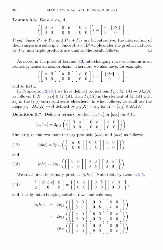
350 MATTHEW NEAL AND BERNARD RUSSO
Lemma 3.6. For a, b, c ∈ A,[0 a0 0
] [0 b0 0
] [0 c0 0
]=[
0 abc0 0
].
Proof. Since P11 + P12 and P12 + P22 are bicontractive, the intersection oftheir ranges is a subtriple. Since A is a JB∗-triple under the product inducedby P12, and triple products are unique, the result follows.
As noted in the proof of Lemma 3.3, interchanging rows or columns is anisometry, hence an isomorphism. Therefore we also have, for example,[
a 00 0
] [b 00 0
] [c 00 0
]=[abc 0
0 0
],
and so forth.In Proposition 2.4(b) we have defined projections Pij : Mn(A) →Mn(A)
as follows: If X = [xkl] ∈Mn(A), then Pij(X) is the element of Mn(A) withxij in the (i, j) entry and zeros elsewhere. In what follows, we shall use themaps pij : Mn(A) → A defined by pij(X) = xij for X = [xkl] ∈Mn(A).
Definition 3.7. Define a ternary product [a, b, c] or [abc] on A by
[a, b, c] = 2p11
([0 a0 0
] [0 b0 0
] [c 00 0
]).
Similarly, define two more ternary products (abc) and 〈abc〉 as follows:
(abc) = 2p11
([a 00 0
] [0 0b 0
] [0 0c 0
])(12)
and
〈abc〉 = 2p11
([0 0c 0
] [0 00 b
] [0 a0 0
]).(13)
We treat first the ternary product [a, b, c]. Note that, by Lemma 3.5,
12
[[a, b, c] 0
0 0
]=[
0 a0 0
] [0 b0 0
] [c 00 0
],(14)
and that by interchanging suitable rows and columns,
[a, b, c] = 2p21
([0 00 a
] [0 00 b
] [0 0c 0
])= 2p12
([a 00 0
] [b 00 0
] [0 c0 0
])= 2p22
([0 0a 0
] [0 0b 0
] [0 00 c
]).

OPERATOR SPACE CHARACTERIZATION OF C*-ALGEBRAS 351
Lemma 3.8. For a, b, c ∈ A,
[a, b, c] + [c, b, a] = 2 abc ,and hence
‖[a, a, a]‖ = ‖a‖3.
Proof. Given a, b, c ∈ A, it follows from Lemma 3.2, Lemmas 3.4-3.6, Defi-nition 3.7 and (6) that there are elements x, y, z, w ∈ A such that x + y =2 abc and[
x yz w
]=[
0 00 0
]+[
[abc]/2 00 0
]+[
0 abc0 0
]+[
[cba]/2 00 0
].
Hence [abc]/2 + [cba]/2 = x = y = abc (and z = w = 0).
We shall see later in Proposition 4.5 that in fact [abc] = (abc) = 〈abc〉.First we shall show the analog of Lemma 3.8 for each of the ternary products(abc) and 〈abc〉. We note that, as above,[
(abc)/2 00 0
]=[
a 00 0
] [0 0b 0
] [0 0c 0
](15)
and [〈abc〉/2 0
0 0
]=[
0 0c 0
] [0 00 b
] [0 a0 0
].
Moreover, by interchanging rows and/or columns,
(abc) = 2p22
([0 00 a
] [0 b0 0
] [0 c0 0
])= 2p12
([0 a0 0
] [0 00 b
] [0 00 c
])= 2p21
([0 0a 0
] [b 00 0
] [c 00 0
])and
〈abc〉 = 2p22
([0 c0 0
] [b 00 0
] [0 0a 0
])(16)
= 2p12
([0 00 c
] [0 0b 0
] [a 00 0
])= 2p21
([c 00 0
] [0 b0 0
] [0 00 a
]).
Proposition 3.9. If A is an operator space such that M2(A)0 is a boundedsymmetric domain (and consequently M2(A) and A are JB∗-triples), then〈abc〉+ 〈cba〉 = 2 abcA and (abc) + (cba) = 2 abcA.
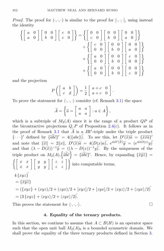
352 MATTHEW NEAL AND BERNARD RUSSO
Proof. The proof for (·, ·, ·) is similar to the proof for [·, ·, ·], using insteadthe identity[
a 0a 0
] [0 0b 0
] [c 0c 0
]=[
0 0c 0
] [0 0b 0
] [0 0a 0
]+[
c 00 0
] [0 0b 0
] [0 0a 0
]+[
a 00 0
] [0 0b 0
] [c 00 0
]+[
a 00 0
] [0 0b 0
] [0 0c 0
]and the projection
P
([a bc d
])=
12
[a+ c 0a+ c 0
].
To prove the statement for 〈·, ·, ·〉 consider (cf. Remark 3.1) the space
A =a =
[a aa a
]: a ∈ A
,
which is a subtriple of M2(A) since it is the range of a product QP ofthe bicontractive projections Q,P of Proposition 2.4(c). It follows as inthe proof of Remark 3.1 that A is a JB∗-triple under the triple product· · ·′ defined by abc′ = 4(abc)e. To see this, let D′(x)a = xxa′
and note that ‖x‖ = 2‖x‖, D′(x)a = 4(D(x)a)e, eitD′(x)y = (e4itD(x)y)eand that (λ − D(x))−1y = ((λ − D(x))−1y)e. By the uniqueness of thetriple product on M2(A),
abc
= abc′. Hence, by expanding xyz =[x xx x
] [y yy y
] [z zz z
]into computable terms,
4 xyze= xyz
= (xyz+ (xyz)/2 + (zyx)/2 + [xyz]/2 + [zyx]/2 + 〈xyz〉/2 + 〈zyx〉/2)e= (3 xyz+ 〈xyz〉/2 + 〈zyx〉/2)e.
This proves the statement for 〈·, ·, ·〉.
4. Equality of the ternary products.
In this section, we continue to assume that A ⊂ B(H) is an operator spacesuch that the open unit ball M2(A)0 is a bounded symmetric domain. Weshall prove the equality of the three ternary products defined in Section 3.
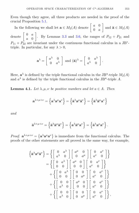
OPERATOR SPACE CHARACTERIZATION OF C*-ALGEBRAS 353
Even though they agree, all three products are needed in the proof of thecrucial Proposition 5.1.
In the following we shall let a ∈M2(A) denote[a 00 a
]and a ∈M2(A)
denote[
0 aa 0
]. By Lemmas 3.3 and 3.6, the ranges of P12 + P21 and
P11 + P22 are invariant under the continuous functional calculus in a JB∗-triple. In particular, for any λ > 0,
aλ =[aλ 00 aλ
]and (a)λ =
[0 aλ
aλ 0
].
Here, aλ is defined by the triple functional calculus in the JB*-triple M2(A)and aλ is defined by the triple functional calculus in the JB*-triple A.
Lemma 4.1. Let λ, µ, ν be positive numbers and let a ∈ A. Then
aλ+µ+ν =aλaµaν
=aλaµaν
=aλaµaν
and
aλ+µ+ν =aλaµaν
=aλaµaν
=aλaµaν
.
Proof. aλ+µ+ν =aλaµaν
is immediate from the functional calculus. The
proofs of the other statements are all proved in the same way, for example,
aλaµaν
=[
0 aλ
aλ 0
] [aµ 00 aµ
] [0 aν
aν 0
]=[
0 aλ
0 0
] [aµ 00 0
] [0 aν
aν 0
]+[
0 aλ
0 0
] [0 00 aµ
] [0 aν
aν 0
]+[
0 0aλ 0
] [aµ 00 0
] [0 aν
aν 0
]+[
0 0aλ 0
] [0 00 aµ
] [0 aν
aν 0
],

354 MATTHEW NEAL AND BERNARD RUSSO
which further expands, using (8)-(11) into
[0 aλ
0 0
] [aµ 00 0
] [0 0aν 0
]+[
0 aλ
0 0
] [0 00 aµ
] [0 0aν 0
]+[
0 0aλ 0
] [aµ 00 0
] [0 aν
0 0
]+[
0 0aλ 0
] [0 00 aµ
] [0 aν
0 0
]=[
0 00 〈aνaµaλ〉/2
]+[〈aλaµaν〉/2 0
0 0
]+[
0 00 〈aλaµaν〉/2
]+[〈aνaµaλ〉/2 0
0 0
]= aλ+µ+ν .
Lemma 4.2. D(a,a) = D(a,a).
Proof. We shall use (3) with z = xxy, which states that
D(xyx , xxy) = 2D(x, yx xxy)−D(x xxyx , y).(17)
We have, by (17) and Lemma 4.1,
D(a,a) = D(
a1/3,a1/3,a1/3,a1/3,a1/3,a1/3
)= 2D
(a1/3,
a1/3,a1/3,
a1/3,a1/3,a1/3
)−D
(a1/3,
a1/3,a1/3,a1/3
,a1/3
,a1/3
)= 2D
(a1/3,
a1/3,a1/3,a
)−D
(a1/3,a,a1/3
,a1/3
)= 2D(a1/3,a5/3)−D(a5/3,a1/3)
= 2D(a,a)−D(a,a),
which proves the lemma.
Lemma 4.3. D(a,a) = D(a,a).

OPERATOR SPACE CHARACTERIZATION OF C*-ALGEBRAS 355
Proof. By Lemma 4.1 and two applications of (1),
D(a,a) = D(
a1/4,a1/4,a1/2,a)
= D(a1/2, a a1/4 a1/4) + [D(a1/4,a1/4), D(a1/2,a)]
= D(a1/2,a3/2) + [D(a1/4,a1/4), D(a1/2,a)]
(by Lemma 4.2 since D(a1/2,a) = D(a3/4,a3/4))
= D(a1/2,a3/2) +D(
a1/4a1/4a1/2,a)−D
(a1/2,
aa1/4a1/4
)= D(a1/2,a3/2) +D(a,a)−D(a1/2,a3/2).
Hence D(a,a)−D(a,a) = D(a1/2,a3/2)−D(a1/2,a3/2).It remains to show that D(a,a3)−D(a,a3) = 0 for every a ∈ A. Now by
(3) and Lemma 4.1,
D(a,a3) = D(a, a,a,a)= D(aaa ,a)/2 +D(a3,a)/2= D(a3,a)/2 +D(a3,a)/2= D(a,a3) (by interchanging a and a).
This proves the lemma.
By linearization from the preceding two lemmas we obtain:
Lemma 4.4. D(a,b) = D(a,b); D(a,b) = D(a,b).
Proof. From D(a + b,a + b) = D(a + b,a + b) follows D(b,a) +D(a,b) =D(a,b)+D(b,a). Now replace a by ia and add to obtain D(a,b) = D(a,b).The second statement follows similarly from D(a+b,a+b) = D(a+b,a+b).
Proposition 4.5. If A is an operator space such that M2(A)0 is a boundedsymmetric domain, then [abc] = (abc) = 〈abc〉.
Proof. By expanding as in the second part of the proof of Lemma 4.3,
D(a,b)[x 00 0
]=
[a 00 a
] [b 00 b
] [x 00 0
]=
[a 00 0
] [b 00 0
] [x 00 0
]=
[abx 0
0 0
]

356 MATTHEW NEAL AND BERNARD RUSSO
and
D(a,b)[x 00 0
]=[
0 aa 0
] [0 bb 0
] [x 00 0
]=[
0 a0 0
] [0 b0 0
] [x 00 0
]+[
0 0a 0
] [0 0b 0
] [x 00 0
]=[
[abx]/2 + (xba)/2 00 0
],
so that [xba] = (xba).Similarly,[
0 〈xba〉/2〈abx〉/2 0
]=[
a 00 a
] [0 bb 0
] [x 00 0
]= D(a,b)
[x 00 0
]= D(a,b)
[x 00 0
]=[
0 aa 0
] [b 00 b
] [x 00 0
]=[
0 [xba]/2(abx)/2 0
],
so that 〈xba〉 = [xba].
5. Main result.
Proposition 5.1. Let X be an operator space such that M2(X)0 is a bound-ed symmetric domain. Then (X, [· · ·], ‖ · ‖) is a C∗-ternary ring in the senseof Zettl [39] (see Definition 2.3) and its JB∗-triple product (see the beginningof Section 3) satisfies abc = ([abc] + [cba])/2.
Proof. It was already shown in Lemma 3.8 that abc = ([abc]+[cba])/2 andthat ‖[aaa]‖ = ‖a‖3 and it is clear that ‖[abc]‖ ≤ ‖a‖‖b‖‖c‖. It remains toshow associativity. To prove this we will use Lemma 3.3 and Proposition 4.5.For a, b, c, d, e ∈ X, let
A =[
0 a0 0
], B =
[0 b0 0
], C =
[c 00 0
], D =
[0 0d 0
], E =
[0 0e 0
].
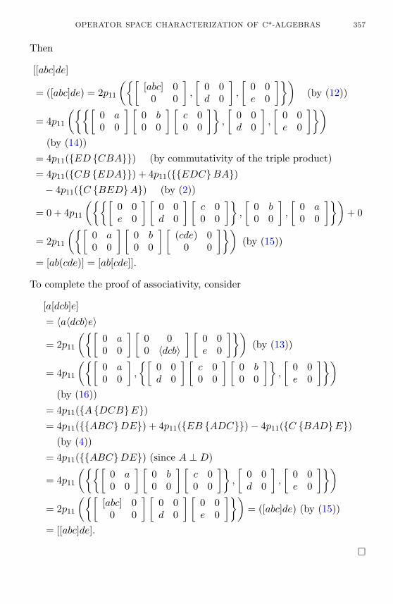
OPERATOR SPACE CHARACTERIZATION OF C*-ALGEBRAS 357
Then
[[abc]de]
= ([abc]de) = 2p11
([[abc] 0
0 0
],
[0 0d 0
],
[0 0e 0
])(by (12))
= 4p11
([0 a0 0
] [0 b0 0
] [c 00 0
],
[0 0d 0
],
[0 0e 0
])(by (14))
= 4p11(ED CBA) (by commutativity of the triple product)
= 4p11(CB EDA) + 4p11(EDCBA)− 4p11(C BEDA) (by (2))
= 0 + 4p11
([0 0e 0
] [0 0d 0
] [c 00 0
],
[0 b0 0
],
[0 a0 0
])+ 0
= 2p11
([0 a0 0
] [0 b0 0
] [(cde) 0
0 0
])(by (15))
= [ab(cde)] = [ab[cde]].
To complete the proof of associativity, consider
[a[dcb]e]
= 〈a〈dcb〉e〉
= 2p11
([0 a0 0
] [0 00 〈dcb〉
] [0 0e 0
])(by (13))
= 4p11
([0 a0 0
],
[0 0d 0
] [c 00 0
] [0 b0 0
],
[0 0e 0
])(by (16))
= 4p11(A DCBE)= 4p11(ABCDE) + 4p11(EB ADC)− 4p11(C BADE)
(by (4))
= 4p11(ABCDE) (since A ⊥ D)
= 4p11
([0 a0 0
] [0 b0 0
] [c 00 0
],
[0 0d 0
],
[0 0e 0
])= 2p11
([[abc] 0
0 0
] [0 0d 0
] [0 0e 0
])= ([abc]de) (by (15))
= [[abc]de].

358 MATTHEW NEAL AND BERNARD RUSSO
Lemma 5.2. Let A be an operator space such that M2(A)0 is a boundedsymmetric domain, so that by Proposition 5.1, A is a C∗-ternary ring. Sup-pose that the C∗-ternary ring A is isomorphic to a TRO, that is, A−1 = 0in Theorem 2.2. Form the ternary product [· · ·]M2(A) induced by the ternaryproduct on A as if it was ordinary matrix multiplication, that is, if X =[xij ], Y = [ykl], Z = [zpq] ∈ M2(A), then [XY Z]M2(A) is the matrix whose(i, j)-entry is
∑p,q[xipyqpzqj ]. Then
2 XY ZM2(A) = [XY Z]M2(A) + [ZY X]M2(A).
Proof. It suffices to prove that XXXM2(A) = [XXX]M2(A). In the firstplace,
[XXX]M2(A) =
[x11x11x11] + [x12x12x11] [x11x11x12] + [x12x12x12]
+[x11x21x21] + [x12x22x21] +[x11x21x22] + [x12x22x22]
[x21x11x11] + [x22x12x11] [x21x11x12] + [x22x12x12]
+[x21x21x21] + [x22x22x21] +[x21x21x22] + [x22x22x22]
.
On the other hand, by using Lemmas 3.3, 3.4, 3.6 and 3.8, and Proposi-tion 3.9,
∑k,l,p,q
P11(X)Pkl(X)Ppq(X)
=
x11x11x11+ [x12x12x11]/2 [x11x11x12]/2
+[x11x21x21]/2 +[x11x21x22]/2
[x21x11x11]/2 + [x22x12x11]/2 0
,
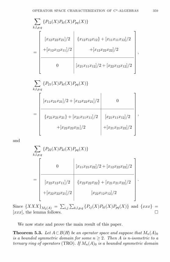
OPERATOR SPACE CHARACTERIZATION OF C*-ALGEBRAS 359∑k,l,p,q
P12(X)Pkl(X)Ppq(X)
=
[x12x22x21]/2 x12x12x12+ [x11x11x12]/2
+[x12x12x11]/2 +[x12x22x22]/2
0 [x21x11x12]/2 + [x22x12x12]/2
,
∑k,l,p,q
P21(X)Pkl(X)Ppq(X)
=
[x11x21x21]/2 + [x12x22x21]/2 0
x21x21x21+ [x21x11x11]/2 [x21x11x12]/2
+[x22x22x21]/2 +[x21x21x22]/2
,
and ∑k,l,p,q
P22(X)Pkl(X)Ppq(X)
=
0 [x11x21x22]/2 + [x12x22x22]/2
[x22x12x11]/2 x22x22x22+ [x21x21x22]/2
+[x22x22x21]/2 [x22x12x12]/2
.
Since XXXM2(A) =∑
i,j
∑k,l,p,q Pij(X)Pkl(X)Ppq(X) and xxx =
[xxx], the lemma follows.
We now state and prove the main result of this paper.
Theorem 5.3. Let A⊂B(H) be an operator space and suppose that Mn(A)0is a bounded symmetric domain for some n ≥ 2. Then A is n-isometric to aternary ring of operators (TRO). If Mn(A)0 is a bounded symmetric domain

360 MATTHEW NEAL AND BERNARD RUSSO
for all n ≥ 2, then A is ternary isomorphic and completely isometric to aTRO.
Proof. The second statement follows from the first one. Suppose n = 2.From Theorem 2.2 and Proposition 5.1, we know that A = A1 ⊕A−1 whereA1 is ternary isomorphic to a TRO B and A−1 is anti-isomorphic to a TROC. Let ϕ : A−1 → C be an anti-isomorphism. Since C is a JB*-triple underthe product x y z = (1/2)(xy∗z + zy∗x) and ϕ is an isometry, hence atriple isomorphism, it follows that
ϕ(x)ϕ(x)∗ϕ(x) = ϕ xxx = ϕ[xxx] = −ϕ(x)ϕ(x)∗ϕ(x)
so that ϕ(x)ϕ(x)∗ϕ(x) = 0 and x = 0. Thus A−1 = 0 and A is ternaryisomorphic to a TRO B. Let ψ : A→ B be a surjective ternary isomorphism.Then by Lemma 5.2, the amplification ψ2 is a triple isomorphism of the JB*-triple M2(A) onto the JB*-triple M2(B), with the triple product
RSTM2(B) := (RS∗T + TS∗R)/2,
implying that ψ2 is a triple isomorphism, hence an isometry. Thus, A is 2-isometric to B, proving the theorem for n = 2. The general case for Mn(A)is now not difficult to obtain. We require only one short lemma.
Lemma 5.4. Let A be an operator space such that for some n ≥ 3, Mn(A)has a JB∗-triple structure. Then for X,Y, Z ∈Mn(A), the following productsall vanish:
• Pij(X) Pkj(Y ) Plj(Z) (for distinct i, k, l)• Pij(X) Pik(Y ) Pil(Z) (for distinct j, k, l)• Pij(X) Pkl(Y ) Ppq(Z) (for i 6= k, j 6= l and either p 6∈ i, k orq 6∈ j, l).
Proof. Two applications of the fact that the range of a bicontractive projec-tion on a JB*-triple is a subtriple yield that Pij(X) Pkj(Y ) Plj(Z) lies in(Pij + Pkj + Plj)Mn(A). However, by a conditional expectation property,
(Pij + Pkj)Pij(X) Pkj(Y ) Plj(Z) = (Pij + Pkj)Pij(X) Pkj(Y ) 0 = 0.
A similar calculation shows (Pkj+Plj)Pij(X) Pkj(Y ) Plj(Z) = 0, provingthe first statement. A similar agrument proves the second statement. Theproof of the last statement is the same as the proof of Lemma 3.3. Forn = 3, one needs to prove, for example, that
D
a 0 00 0 00 0 0
, 0 0 0
0 b 00 0 0
= 0.

OPERATOR SPACE CHARACTERIZATION OF C*-ALGEBRAS 361
Returning to the proof of Theorem 5.3, if Mn(A) is a JB*-triple, thenM2(A), which is isometric to the range of a contractive projection onMn(A),is also a JB*-triple. Hence, by the n = 2 case, A is a C∗-ternary ringwhich is ternary isomorphic and isometric under a map φ to a TRO B andM2(A) is triple isomorphic and isometric to M2(B) under the amplificationφ2. Every triple product XY Z in Mn(A) is the sum of products of theform Pij(X) Pkl(Y ) Ppq(Z). By Lemma 5.4, every such product of matrixelements inMn(A) is either zero or takes place in the intersection of two rowswith two columns. The subspace ofMn(A) defined by one such intersection isa subtriple of Mn(A) since it is the range of the product of two bicontractiveprojections. It is isometric, via
Pij(X) + Pil(Y ) + Pkj(Z) + Pkl(W ) 7→[Pij(X) Pil(Y )Pkj(Z) Pkl(W )
],
hence triple isomorphic, to M2(A). Hence, by the proof of the n = 2 case,all triple products in Mn(A) are the natural ones obtained from the ternarystructure on A as in Lemma 5.2. It follows that Mn(A) is triple isomorphicto Mn(B) via the amplification map φn which is thus an isometry.
As application, we offer two corollaries.
Corollary 5.5. Let A ⊂ B(H,K) be a TRO and let P be a completelycontractive projection on A. Then the range of P is completely isometric toanother TRO.
Proof. Since A is a TRO, Mn(A) is a JB*-triple. Therefore Mn(P (A)) =Pn(Mn(A)) is a JB*-triple, and its unit ball is a bounded symmetric domain.
Another way to obtain this corollary is to note that every TRO is a cornerof a C∗-algebra and hence the range of a completely contractive projection onthat algebra. By composing these two projections, the corollary is reducedto [38].
Our second corollary is a variant of the fundamental Choi-Effros result.
Corollary 5.6. Let P be a unital 2-positive projection on a unital C∗-algebra A. Then P (A) is 2-isometric to a C∗-algebra. If P is completelypositive and unital, then P (A) is completely isometric to a C∗-algebra.
In order to state our second theorem, we recall that a complex Banachspace A is linearly isometric to a unital JB*-algebra if and only if its openunit ball A0 is a bounded symmetric domain of tube type [11]. In [37], anecessary and sufficient condition, involving the Lie algebra of all completeholomorphic vector fields on A0, is given for such A to be obtained froma C∗-algebra with the anticommutator product. Our next theorem gives aholomorphic characterization of C∗-algebras up to complete isometry.

362 MATTHEW NEAL AND BERNARD RUSSO
Theorem 5.7. Let A⊂B(H) be an operator space and suppose that Mn(A)0is a bounded symmetric domain for some n ≥ 2. If the induced boundedsymmetric domain structure on A0 is of tube type, then A is n-isometric toa C∗-algebra. If Mn(A)0 is a bounded symmetric domain for all n ≥ 2 andA0 is of tube type, then A is completely isometric to a C∗-algebra.
Proof. By Theorem 5.3, we may assume that A is a TRO. Since A hasthe structure of a unital JB*-algebra, there is a partial isometry u ∈ Asuch that au∗u = uu∗a = a for every a ∈ A. Then A becomes a C∗-algebra with product a · b = au∗b and involution a] = ua∗u. Since ab∗c =a · b] · c, and ternary isomorphisms of TRO’s are complete isometries, theresult follows.
Remark 5.8. One can construct operator spaces that are 2-isometric to aC∗-algebra A which are not completely isometric to A. Hence, if M2(A)0 isa bounded symmetric domain it does not follow that Mn(A)0 is a boundedsymmetric domain for every n ≥ 2. It would be interesting to see if this weretrue under some further condition on A. The proof of Theorem 5.3 seemsto require a bounded symmetric domain structure on M2(A)0, not simplyon M1,2(A)0 for example. It would be interesting to see what could be saidif it is assumed that M1,n(A)0 were a bounded symmetric domain for everyn ≥ 2.
Acknowledgements. The authors wish to thank Profesors Zhong-Jin Ruanand David Blecher for their advice and encouragement at the beginningstages of this work.
References
[1] K. El Amin, A.M. Campoy and A.R. Palacios, A holomorphic characterizationof C∗- and JB∗-algebras, Manu. Math., 104 (2001), 467-478, MR 2002e:46085,Zbl 0982.46040.
[2] J. Arazy and Y. Friedman, Contractive projections in C1 and C∞, Mem. Amer. Math.Soc., 13(200), 1978, MR 82b:47023, Zbl 0382.47020.
[3] W.B. Arveson, Subalgebras of C∗-algebras, Acta Math., 123 (1969), 141-224,MR 40 #6274, Zbl 0194.15701.
[4] , Subalgebras of C∗-algebras II, Acta Math., 128 (1972), 271-308,MR 52 #15035, Zbl 0245.46098.
[5] T.J. Barton and R. Timoney, On biduals, preduals and ideals of JB∗-triples, Math.Scand., 59 (1986), 177-191.
[6] D. Blecher, The standard dual of an operator space, Pacific J. Math., 153 (1992),15-30, MR 93d:47083, Zbl 0726.47030.
[7] , A completely bounded characterization of operator algebras, Math. Ann., 303(1995), 227-239, MR 96k:46098, Zbl 0892.47048.
[8] , The Shilov boundary of an operator space and the characterization theorems,J. Funct. Anal., 182 (2001), 280-343, MR 2002d:46049.

OPERATOR SPACE CHARACTERIZATION OF C*-ALGEBRAS 363
[9] D. Blecher and V. Paulsen, Multipliers of operator spaces and the injective envelope,Pacific J. Math., 200 (2001), 1-17, MR 2002k:46150.
[10] D. Blecher, Z.-J. Ruan and A. Sinclair, A characterization of operator algebras, J.Funct. Anal., 89 (1990), 188-201, MR 91b:47098, Zbl 0714.46043.
[11] R. Braun, W. Kaup and H. Upmeier, A holomorphic characterization of Jordan C∗-algebras, Math. Zeit., 161 (1978), 277-290, MR 58 #12398, Zbl 0385.32002.
[12] M.-D. Choi and E. Effros, Injectivity and operator spaces, J. Funct. Anal., 24 (1977),156-209, MR 55 #3814, Zbl 0341.46049.
[13] C-H. Chu, M. Neal and B. Russo, Normal contractive projections preserve type.Preprint, 2001.
[14] S. Dineen, The second dual of a JB∗-triple system, in ‘Complex Analysis, FunctionalAnalysis and Approximation Theory’, J. Mujica (ed.), Amsterdam: Elsevier (NorthHolland), 1986, 67-69, MR 88f:46097, Zbl 0653.46053.
[15] E. Effros, N. Ozawa and Z.-J. Ruan, On injectivity and nuclearity for operator spaces,Duke Math. J., 110 (2001), 489-521, MR 2002k:46151.
[16] E. Effros and Z.J. Ruan, Operator Spaces, Oxford University Press, 2000,MR 2002a:46082, Zbl 0969.46002.
[17] E. Effros and E. Stormer, Positive projections and Jordan structure in operator alge-bras, Math. Scand., 45 (1979), 127-138, MR 82e:46076, Zbl 0455.46059.
[18] Y. Friedman and B. Russo, Contractive projections on C0(K), Trans. Amer. Math.Soc., 273 (1982), 57-73, MR 83i:46062, Zbl 0534.46037.
[19] , Function representation of commutative operator triple systems, J. Lon.Math. Soc. (2), 27 (1983), 513-524, MR 84h:46095, Zbl 0543.46046.
[20] , Conditional expectation without order, Pacific J. Math., 115 (1984), 351-360,MR 86b:46116, Zbl 0563.46039.
[21] , Solution of the contractive projection problem, J. Funct. Anal., 60 (1985),56-79, MR 87a:46115, Zbl 0558.46035.
[22] , Structure of the predual of a JBW∗-triple, J. Reine Angew. Math., 356(1985), 67-89, MR 86f:46073, Zbl 0547.46049.
[23] M. Hamana, Injective envelopes of operator systems, Publ. Res. Inst. Math. Sci. KyotoUniv., 15 (1979), 773-785, MR 81h:46071, Zbl 0436.46046.
[24] , Triple envelopes and Silov boundaries of operator spaces, Math. J. ToyamaUniv., 22 (1999), 77-93, MR 2001a:46057.
[25] L.A. Harris, Bounded symmetric domains in infinite dimensional spaces, in ‘Infi-nite Dimensional Holomorphy’ (T.L. Hayden and T.J. Suffridge, eds.), Proceedings,1973, Lecture Notes in Mathematics, 364, 13-40, Springer, 1974, MR 53 #11106,Zbl 0293.46049.
[26] G. Horn, Classification of JBW∗-triples of Type I, Math. Zeit., 196 (1987), 271-291,MR 88m:46076, Zbl 0615.46045.
[27] G. Horn and E. Neher, Classification of continuous JBW∗-triples, Trans. Amer. Math.Soc., 306 (1988), 553-578, MR 89c:46090, Zbl 0659.46063.
[28] W. Kaup, A Riemann mapping theorem for bounded symmetric domains in complexBanach spaces, Math. Zeit., 183 (1983), 503-529, MR 85c:46040, Zbl 0519.32024.
[29] , Contractive projections on Jordan C∗-algebras and generalizations, Math.Scand., 54 (1984), 95-100, MR 85h:17012, Zbl 0578.46066.

364 MATTHEW NEAL AND BERNARD RUSSO
[30] Y. Lindenstrauss and D. Wulbert, On the classification of Banach spaces whose dualsare L1-spaces, J. Funct. Anal., 4 (1969), 332-349, MR 40 #3274, Zbl 0184.15102.
[31] O. Loos, Bounded symmetric domains and Jordan pairs, Lecture Notes, Univ. ofCalifornia, Irvine, 1977.
[32] M. Neal and B. Russo, Contractive projections and operator spaces, C.R. Acad. Sci.Paris, 331 (2000), 873-878, MR 2001m:46128, Zbl 0973.47052.
[33] , Contractive projections and operator spaces, Trans. Amer. Math. Soc. (toappear).
[34] Z.-J. Ruan, Subspaces of C∗-algebras, J. Funct. Anal., 76 (1988), 217-230,MR 89h:46082, Zbl 0646.46055.
[35] , Injectivity of operator spaces, Trans. Amer. Math. Soc., 315 (1989), 89-104,MR 91d:46078, Zbl 0669.46029.
[36] B. Russo, Structure of JB∗-triples, in ‘Jordan Algebras’, Proc. Oberwolfach Confer-ence 1992 (W. Kaup, K. McCrimmon, H. Petersson, Eds.), de Gruyter, Berlin, 1994,209-280, MR 95h:46109, Zbl 0805.46072.
[37] H. Upmeier, A holomorphic characterization of C∗-algebras, in ‘Functional Analysis,holomorphy and approximation theory, II’ (Rio de Janeiro, 1981), North HollandMath. Stud., 86 (1984), 427-467, MR 86k:46089, Zbl 0546.46050.
[38] M.A. Youngson, Completely contractive projections on C∗-algebras, Quart. J. Math.,34 (1983), 507-511, MR 85f:46112, Zbl 0542.46029.
[39] H. Zettl, A characterization of ternary rings of operators, Adv. Math., 48 (1983),117-143, MR 84h:46093, Zbl 0517.46049.
Received November 22, 2001 and revised April 25, 2002. Both authors acknowledge thesupport of NSF Grant DMS-0101153.
Department of MathematicsDenison UniversityGranville, OH 43023E-mail address: [email protected]
Department of MathematicsUniversity of CaliforniaIrvine, CA 92697-3875E-mail address: [email protected]

PACIFIC JOURNAL OF MATHEMATICSVol. 209, No. 2, 2003
ON THE VERE–JONES CLASSIFICATION ANDEXISTENCE OF MAXIMAL MEASURES FOR
COUNTABLE TOPOLOGICAL MARKOV CHAINS
Sylvie Ruette
We consider topological Markov chains (also called Markovshifts) on countable graphs. We show that a transient graphcan be extended to a recurrent graph of equal entropy whichis either positive recurrent of null recurrent, and we give anexample of each type. We extend the notion of local entropy totopological Markov chains and prove that a transitive Markovchain admits a measure of maximal entropy (or maximal mea-sure) whenever its local entropy is less than its (global) en-tropy.
Introduction.
In this article we are interested in connected oriented graphs and topologicalMarkov chains. All the graphs we consider have a countable set of vertices.If G is an oriented graph, let ΓG be the set of two-sided infinite sequencesof vertices that form a path in G and let σ denote the shift transformation.The Markov chain associated to G is the (noncompact) dynamical system(ΓG, σ). The entropy h(G) of the Markov chain ΓG was defined by Gurevich;it can be computed by several ways and satisfies the Variational Principle[7] and [8].
In [16] Vere-Jones classifies connected oriented graphs as transient, nullrecurrent or positive recurrent according to the properties of the series as-sociated with the number of loops, by analogy with probabilistic Markovchains. To a certain extent, positive recurrent graphs resemble finite graphs.In [7] Gurevich shows that a Markov chain on a connected graph admits ameasure of maximal entropy (also called maximal measure) if and only ifthe graph is positive recurrent. In this case, this measure is unique and itis an ergodic Markov measure.
In [13] and [14] Salama gives a geometric approach to the Vere-Jonesclassification. The fact that a graph can (or cannot) be “extended” or“contracted” without changing its entropy is closely related to its class. Inparticular a graph with no proper subgraph of equal entropy is positiverecurrent. The converse is not true [14] (see also [6] for an example ofa positive recurrent graph with a finite valency at every vertex that has
365

366 SYLVIE RUETTE
no proper subgraph of equal entropy). This result shows that the positiverecurrent class splits into two subclasses: A graph is called strongly positiverecurrent if it has no proper subgraph of equal entropy; it is equivalent to acombinatorial condition (a finite connected graph is always strongly positiverecurrent). In [13] and [14] Salama also states that a graph is transient ifand only if it can be extended to a bigger transient graph of equal entropy.We show that any transient graph G is contained in a recurrent graph ofequal entropy, which is positive or null recurrent depending on the propertiesof G. We illustrate the two possibilities — a transient graph with a positiveor null recurrent extension — by an example.
The result of Gurevich entirely solves the question of existence of a max-imal measure in term of graph classification. Nevertheless it is not so easyto prove that a graph is positive recurrent and one may wish to have moreefficient criteria. In [10] Gurevich and Zargaryan give a sufficient conditionfor existence of a maximal measure; it is formulated in terms of exponentialgrowth of the number of paths inside and outside a finite subgraph. We givea new sufficient criterion based on local entropy.
Why consider local entropy? For a compact dynamical system, it is knownthat a null local entropy implies the existence of a maximal measure ([11], seealso [1] for a similar but different result). This result may be strengthened insome cases: It is conjectured that, if f is a map of the interval which is Cr,r > 1, and satisfies htop(f) > hloc(f), then there exists a maximal measure[2]. Our initial motivation comes from the conjecture above because smoothinterval maps and Markov chains are closely related. If f : [0, 1] → [0, 1]is C1+α (i.e., f is C1 and f ′ is α-Holder with α > 0) with htop(f) > 0then an oriented graph G can be associated to f , G is connected if f istransitive, and there is a bijection between the maximal measures of f andthose of ΓG [2] and [3]. We show that a Markov chain is strongly positiverecurrent, thus admits a maximal measure, if its local entropy is strictly lessthat its Gurevich entropy. However this result does not apply directly tointerval maps since the “isomorphism” between f and its Markov extensionis not continuous so it may not preserve local entropy (which depends onthe distance).
The article is organized as follows. Section 1 contains definitions andbasic properties on oriented graphs and Markov chains. In Section 2, afterrecalling the definitions of transient, null recurrent and positive recurrentgraphs and some related properties, we show that any transient graph iscontained in a recurrent graph of equal entropy (Proposition 2.8) and wegive an example of a transient graph which extends to a positive recurrent(resp. null recurrent) graph. Section 3 is devoted to the problem of exis-tence of maximal measures: Theorem 3.8 gives a sufficient condition for theexistence of a maximal measure, based on local entropy.

CLASSIFICATION AND MAXIMAL MEASURES 367
1. Background.
1.1. Graphs and paths. Let G be an oriented graph with a countable setof vertices V (G). If u, v are two vertices, there is at most one arrow u→ v.A path of length n is a sequence of vertices (u0, . . . , un) such that ui → ui+1
in G for 0 ≤ i < n. This path is called a loop if u0 = un. We say that thegraph G is connected if for all vertices u, v there exists a path from u to v;in the literature, such a graph is also called strongly connected.
If H is a subgraph of G, we write H ⊂ G; if in addition H 6= G, we writeH ⊆/ G and say that H is a proper subgraph. If W is a subset of V (G),the set V (G) \W is denoted by W . We also denote by W the subgraph ofG whose vertices are W and whose edges are all edges of G between twovertices in W .
Let u, v be two vertices. We define the following quantities:• pGuv(n) is the number of paths (u0, . . . , un) such that u0 = u and un = v;Ruv(G) is the radius of convergence of the series
∑pGuv(n)zn.
• fGuv(n) is the number of paths (u0, . . . , un) such that u0 = u, un = vand ui 6= v for 0 < i < n; Luv(G) is the radius of convergence of theseries
∑fGuv(n)zn.
Proposition 1.1 (Vere-Jones [16]). Let G be an oriented graph. If G isconnected, Ruv(G) does not depend on u and v; it is denoted by R(G).
If there is no confusion, R(G) and Luv(G) will be written R and Luv. Fora graph G′ these two radii will be written R′ and L′uv.
1.2. Markov chains. Let G be an oriented graph. ΓG is the set of two-sided infinite paths in G, that is,
ΓG = (vn)n∈Z | ∀n ∈ Z, vn → vn+1 in G ⊂ (V (G))Z.
σ is the shift on ΓG. The (topological) Markov chain on the graph G is thesystem (ΓG, σ).
The set V (G) is endowed with the discrete topology and ΓG is endowedwith the induced topology of (V (G))Z. The space ΓG is not compact unlessG is finite. A compatible distance on ΓG is given by d, defined as follows:V (G) is identified with N and the distance D on V (G) is given by D(n,m) =∣∣ 12n − 1
2m
∣∣. If u = (un)n∈Z and v = (vn)n∈Z are two elements of ΓG,
d(u, v) =∑n∈Z
D(un, vn)2|n|
≤ 3.
The Markov chain (ΓG, σ) is transitive if for any nonempty open setsA,B ⊂ ΓG there exists n > 0 such that σn(A) ∩B 6= ∅. Equivalently, ΓG istransitive if and only if the graph G is connected. In the sequel we will beinterested in connected graphs only.

368 SYLVIE RUETTE
1.3. Entropy. If G is a finite graph, ΓG is compact and the topologicalentropy htop(ΓG, σ) is well-defined (see e.g., [5] for the definition of thetopological entropy). If G is a countable graph, the Gurevich entropy [7] ofG is given by
h(G) = suphtop(ΓH , σ) | H ⊂ G,H finite.This entropy can also be computed in a combinatorial way, as the expo-
nential growth of the number of paths with fixed endpoints [8].
Proposition 1.2 (Gurevich). Let G be a connected oriented graph. Thenfor any vertices u, v
h(G) = limn→+∞
1n
log pGuv(n) = − logR(G).
Another way to compute the entropy is to compactify the space ΓG andthen use the definition of topological entropy for compact metric spaces. IfG is an oriented graph, denote the one-point compactification of V (G) byV (G) ∪ ∞ and define ΓG as the closure of ΓG in (V (G) ∪ ∞)Z. Thedistance d naturally extends to ΓG. In [7] Gurevich shows that this givesthe same entropy; this means that there is only very little dynamics addedin this compactification. Moreover, the Variational Principle is still valid forMarkov chains [7].
Theorem 1.3 (Gurevich). Let G be an oriented graph. Then
h(G) = htop(ΓG, σ) = suphµ(ΓG) | µ σ-invariant probability measure.
2. On the classification of connected graphs.
2.1. Transient, null recurrent, positive recurrent graphs. In [16]Vere-Jones gives a classification of connected graphs as transient, null re-current or positive recurrent. The definitions are given in Table 1 (lines 1and 2) as well as properties of the series
∑pGuv(n)zn which give an alterna-
tive definition.In [13] and [14] Salama studies the links between the classification and
the possibility to extend or contract a graph without changing its entropy.It follows that a connected graph is transient if and only if it is strictlyincluded in a connected graph of equal entropy, and that a graph with noproper subgraph of equal entropy is positive recurrent.
Remark 2.1. In [13] Salama claims that Luu is independent of u, which isnot true; in [14] he uses the quantity L = infu Luu and he states that ifR = Lthen R = Luu for all vertices u, which is wrong too (see Proposition 3.2in [9]). It follows that in [13] and [14] the statement “R=L” must beinterpreted either as “R = Luu for some u” or “R = Luu for all u” dependingon the context. This encouraged us to give the proofs of Salama’s results inthis article.
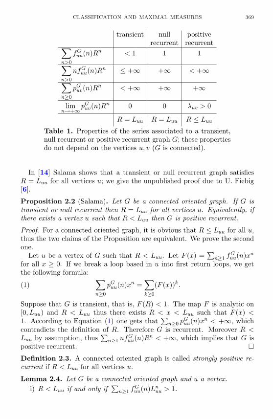
CLASSIFICATION AND MAXIMAL MEASURES 369
transient null positiverecurrent recurrent∑
n>0
fGuu(n)Rn < 1 1 1∑n>0
nfGuu(n)Rn ≤ +∞ +∞ < +∞∑n≥0
pGuv(n)Rn < +∞ +∞ +∞
limn→+∞
pGuv(n)Rn 0 0 λuv > 0
R = Luu R = Luu R ≤ Luu
Table 1. Properties of the series associated to a transient,null recurrent or positive recurrent graph G; these propertiesdo not depend on the vertices u, v (G is connected).
In [14] Salama shows that a transient or null recurrent graph satisfiesR = Luu for all vertices u; we give the unpublished proof due to U. Fiebig[6].
Proposition 2.2 (Salama). Let G be a connected oriented graph. If G istransient or null recurrent then R = Luu for all vertices u. Equivalently, ifthere exists a vertex u such that R < Luu then G is positive recurrent.
Proof. For a connected oriented graph, it is obvious that R ≤ Luu for all u,thus the two claims of the Proposition are equivalent. We prove the secondone.
Let u be a vertex of G such that R < Luu. Let F (x) =∑
n≥1 fGuu(n)xn
for all x ≥ 0. If we break a loop based in u into first return loops, we getthe following formula: ∑
n≥0
pGuu(n)xn =∑k≥0
(F (x))k.(1)
Suppose that G is transient, that is, F (R) < 1. The map F is analytic on[0, Luu) and R < Luu thus there exists R < x < Luu such that F (x) <1. According to Equation (1) one gets that
∑n≥0 p
Guu(n)xn < +∞, which
contradicts the definition of R. Therefore G is recurrent. Moreover R <Luu by assumption, thus
∑n≥1 nf
Guu(n)Rn < +∞, which implies that G is
positive recurrent.
Definition 2.3. A connected oriented graph is called strongly positive re-current if R < Luu for all vertices u.
Lemma 2.4. Let G be a connected oriented graph and u a vertex.i) R < Luu if and only if
∑n≥1 f
Guu(n)Lnuu > 1.
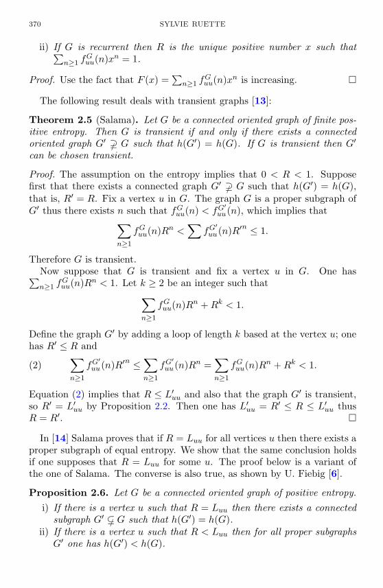
370 SYLVIE RUETTE
ii) If G is recurrent then R is the unique positive number x such that∑n≥1 f
Guu(n)xn = 1.
Proof. Use the fact that F (x) =∑
n≥1 fGuu(n)xn is increasing.
The following result deals with transient graphs [13]:
Theorem 2.5 (Salama). Let G be a connected oriented graph of finite pos-itive entropy. Then G is transient if and only if there exists a connectedoriented graph G′ ⊇/ G such that h(G′) = h(G). If G is transient then G′
can be chosen transient.
Proof. The assumption on the entropy implies that 0 < R < 1. Supposefirst that there exists a connected graph G′ ⊇/ G such that h(G′) = h(G),that is, R′ = R. Fix a vertex u in G. The graph G is a proper subgraph ofG′ thus there exists n such that fGuu(n) < fG
′uu(n), which implies that∑
n≥1
fGuu(n)Rn <∑
fG′
uu(n)R′n ≤ 1.
Therefore G is transient.Now suppose that G is transient and fix a vertex u in G. One has∑n≥1 f
Guu(n)Rn < 1. Let k ≥ 2 be an integer such that∑
n≥1
fGuu(n)Rn +Rk < 1.
Define the graph G′ by adding a loop of length k based at the vertex u; onehas R′ ≤ R and∑
n≥1
fG′
uu(n)R′n ≤∑n≥1
fG′
uu(n)Rn =∑n≥1
fGuu(n)Rn +Rk < 1.(2)
Equation (2) implies that R ≤ L′uu and also that the graph G′ is transient,so R′ = L′uu by Proposition 2.2. Then one has L′uu = R′ ≤ R ≤ L′uu thusR = R′.
In [14] Salama proves that if R = Luu for all vertices u then there exists aproper subgraph of equal entropy. We show that the same conclusion holdsif one supposes that R = Luu for some u. The proof below is a variant ofthe one of Salama. The converse is also true, as shown by U. Fiebig [6].
Proposition 2.6. Let G be a connected oriented graph of positive entropy.i) If there is a vertex u such that R = Luu then there exists a connected
subgraph G′ ⊆/ G such that h(G′) = h(G).ii) If there is a vertex u such that R < Luu then for all proper subgraphs
G′ one has h(G′) < h(G).
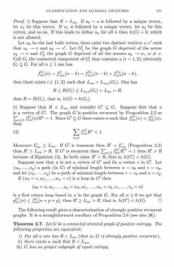
CLASSIFICATION AND MAXIMAL MEASURES 371
Proof. i) Suppose that R = Luu. If u0 = u is followed by a unique vertex,let u1 be this vertex. If u1 is followed by a unique vertex, let u2 be thisvertex, and so on. If this leads to define un for all n then h(G) = 0, whichis not allowed.
Let uk be the last built vertex; there exist two distinct vertices v, v′ suchthat uk → v and uk → v′. Let G′1 be the graph G deprived of the arrowuk → v and G′2 the graph G deprived of all the arrows uk → w, w 6= v.Call Gi the connected component of G′i that contains u (i = 1, 2); obviouslyGi ⊆/ G. For all n ≥ 1 one has
fGuu(n) = fGuku(n− k) = fG1
uku(n− k) + fG2
uku(n− k),
thus there exists i ∈ 1, 2 such that Luu = Luku(Gi). One has
R ≤ R(Gi) ≤ Luku(Gi) = Luu = R,
thus R = R(Gi), that is, h(G) = h(Gi).
ii) Suppose that R < Luu and consider G′ ⊆/ G. Suppose first that uis a vertex of G′. The graph G is positive recurrent by Proposition 2.2 so∑
n≥1 fGuu(n)Rn = 1. Since G′ ⊆/ G there exists n such that fG
′uu(n) < fGuu(n),
thus ∑n≥1
fG′
uuRn < 1.(3)
Moreover L′uu ≥ Luu. If G′ is transient then R′ = L′uu (Proposition 2.2)thus R′ ≥ Luu > R. If G′ is recurrent then
∑n≥1 f
G′uuR
′n = 1 thus R′ > R
because of Equation (3). In both cases R′ > R, that is, h(G′) < h(G).Suppose now that u is not a vertex of G′ and fix a vertex v in G′. Let
(u0, . . . , up) a path (in G) of minimal length between u = u0 and v = up,and let (v0, . . . , vq) be a path of minimal length between v = v0 and u = vq.
If (w0 = v, w1, . . . , wn = v) is a loop in G′ then
(u0 = u, u1, . . . , up = w0, w1, . . . , wn = v0, v1, . . . , vq = u)
is a first return loop based in u in the graph G. For all n ≥ 0 we get thatpG
′vv(n) ≤ fGuu(n+ p+ q), thus R′ ≥ Luu > R, that is, h(G′) < h(G).
The following result gives a characterization of strongly positive recurrentgraphs. It is a straightforward corollary of Proposition 2.6 (see also [6]).
Theorem 2.7. Let G be a connected oriented graph of positive entropy. Thefollowing properties are equivalent:
i) For all u one has R < Luu (that is, G is strongly positive recurrent ),ii) there exists u such that R < Luu,iii) G has no proper subgraph of equal entropy.

372 SYLVIE RUETTE
2.2. Recurrent extensions of equal entropy of transient graphs.We show that any transient graph G can be extended to a recurrent graphwithout changing the entropy by adding a (possibly infinite) number ofloops. If the series
∑nfGvv(n)Rn is finite then the obtained recurrent graph
is positive recurrent (but not strongly positive recurrent), otherwise it is nullrecurrent.
Proposition 2.8. Let G be a transient graph of finite positive entropy.Then there exists a recurrent graph G′ ⊃ G such that h(G) = h(G′). More-over G′ can be chosen to be positive recurrent if
∑n>0 nf
Guu(n)Rn < +∞
for some vertex u of G, and G′ is necessarily null recurrent otherwise.
Proof. The entropy of G is finite and positive thus 0 < R < 1 and thereexists an integer p such that 1
2 ≤ pR < 1. Define α = pR. Let u be a vertexof G and define D = 1−
∑n≥1 f
Guu(n)Rn; one has 0 < D < 1. Moreover∑
n≥1
αn ≥∑n≥1
12n
= 1,
thus ∑n≥k+1
αn = αk∑n≥1
αn ≥ αk.(4)
We build a sequence of integers (ni)i∈I such that 2∑
i∈I αni = D. For
this, we define inductively a strictly increasing (finite or infinite) sequenceof integers (ni)i∈I such that for all k ∈ I
k∑i=0
αni ≤ D
2<
k∑i=0
αni +∑n>nk
αn.
— Let n0 be the greatest integer n ≥ 2 such that∑
k≥n αk > D
2 . By choiceof n0 one has
∑n≥n0+1 α
n ≤ D2 , thus αn0 ≤ D
2 by Equation (4). This is therequired property at rank 0.— Suppose that (n0, . . . , nk) is already defined. If
∑ki=0 α
ni = D2 then
I = 0, . . . , k and we stop the construction. Otherwise let nk+1 be thegreatest integer n > nk such that
k∑i=0
αni +∑j≥n
αj >D
2.
By choice of nk+1 and Equation (4), one has
αnk+1 ≤∑
j≥nk+1+1
αj ≤ D
2−
k∑i=0
αni .
This is the required property at rank k + 1.

CLASSIFICATION AND MAXIMAL MEASURES 373
Define a new graph G′ ⊃ G by adding 2pni loops of length ni based at thevertex u. Obviously one has R′ ≤ R, and
∑i∈I(pR)ni = D
2 by construction.Therefore ∑
n≥1
fG′
uu(n)Rn =∑n≥1
fGuu(n)Rn +∑i∈I
2(pR)ni = 1.(5)
This implies that R ≤ L′uu. If G′ is transient then∑
n≥1 fG′uu(n)R′n < 1
and R′ = L′uu by Proposition 2.2, thus R ≤ R′ and Equation (5) leads to acontradiction. Therefore G′ is recurrent. By Lemma 2.4(ii) one has R′ = R,that is, h(G′) = h(G). In addition,∑
n≥1
nfG′
uu(n)Rn =∑n≥1
nfGuu(n)Rn +∑i∈I
niαni
and this quantity is finite if and only if∑nfGuu(n)Rn is finite. In this case
the graph G′ is positive recurrent.
If∑nfGuu(n)Rn = +∞, let H be a recurrent graph containing G with
h(H) = h(G). Then H is null recurrent because∑n≥1
nfHuu(n)Rn ≥∑n≥1
nfGuu(n)Rn = +∞.
Example 2.9. We build a positive (resp. null) recurrent graph G such that∑fGuu(n)Lnuu = 1 and then we delete an arrow to obtain a graph G′ ⊂ G
which is transient and such that h(G′) = h(G). First we give a descriptionof G depending on a sequence of integers a(n) then we give two differentvalues to the sequence a(n) so as to obtain a positive recurrent graph in onecase and a null recurrent graph in the other case.
Let u be a vertex and a(n) a sequence of nonnegative integers for n ≥ 1,with a(1) = 1. The graph G is composed of a(n) loops of length n based atthe vertex u for all n ≥ 1 (see Figure 1). More precisely, define the set ofvertices of G as
V = u ∪+∞⋃n=1
vn,ik | 1 ≤ i ≤ a(n), 1 ≤ k ≤ n− 1,
where the vertices vn,ik above are distinct. Let vn,i0 = vn,in = u for 1 ≤ i ≤a(n). There is an arrow vn,ik → vn,ik+1 for 0 ≤ k ≤ n− 1, 1 ≤ i ≤ a(n), n ≥ 1and there is no other arrow in G. The graph G is connected and fGuu(n) =a(n) for n ≥ 1.
The sequence (a(n))n≥2 is chosen such that it satisfies∑n≥1
a(n)Ln = 1,(6)

374 SYLVIE RUETTE
u
Figure 1. The graphs G and G′; the bold loop (on the left)is the only arrow that belongs to G and not to G′, otherwisethe two graphs coincide.
where L = Luu > 0 is the radius of convergence of the series∑a(n)zn. If G
is transient then R = Luu by Proposition 2.2, but Equation (6) contradictsthe definition of transient. Thus G is recurrent. Moreover, R = L byLemma 2.4(ii).
The graph G′ is obtained from G by deleting the arrow u→ u. Obviouslyone has L′uu = L and ∑
n≥1
fG′
uu(n)Ln = 1− L < 1.
This implies that G′ is transient because R′ ≤ L′uu. Moreover R′ = L′uu byProposition 2.2 thus R′ = R, that is, h(G′) = h(G).
Now we consider two different sequences a(n).
1) Let a(n2) = 2n2−n for n ≥ 1 and a(n) = 0 otherwise. Then L = 1
2 and∑n≥1
fGuu(n)Ln =∑n≥1
2n2−n 1
2n2 =∑n≥1
12n
= 1.
Moreover ∑n≥1
nfGuu(n)Ln =∑n≥1
n2
2n< +∞,
hence the graph G is positive recurrent.
2) Let a(1) = 1, a(2n) = 22n−n for n ≥ 2 and a(n) = 0 otherwise. One cancompute that L = 1
2 , and∑n≥1
fGuu(n)Ln =12
+∑n≥2
22n−n 122n =
12
+∑n≥2
12n
= 1.
Moreover ∑n≥1
nfGuu(n)Ln =12
+∑n≥2
2n12n
= +∞

CLASSIFICATION AND MAXIMAL MEASURES 375
hence the graph G is null recurrent.
Remark 2.10. Let G be a transient graph of finite entropy. Fix a vertex uand choose an integer k such that
∑n≥k R
n < 1−∑
n≥1 fGuu(n)Rn. For every
integer n ≥ k let mn = bR−nc, add bR−(mn−n)c loops of length mn basedat the vertex u and call G′ the graph obtained in this way. It can be shownthat the graph G′ is transient, h(G′) = h(G) and
∑n≥1 nf
G′uuR
′n = +∞.Then Proposition 2.8 implies that every transient graph is included in a nullrecurrent graph of equal entropy.
Remark 2.11. In the more general setting of thermodynamic formalismfor countable Markov chains, Sarig puts to the fore a subclass of positiverecurrent potentials which he calls strongly positive recurrent [15]; his moti-vation is different, but the classifications agree. If G is a countable orientedgraph, a potential is a continuous map φ : ΓG → R and the pressure P (φ)is the analogous of the Gurevich entropy, the paths being weighted by eφ;a potential is either transient or null recurrent or positive recurrent. Con-sidering the null potential φ ≡ 0, we retrieve the case of (non-weighted)topological Markov chains. In [15] Sarig introduces a quantity ∆u[φ]; φ istransient (resp. recurrent) if ∆u[φ] < 0 (resp. ∆u[φ] ≥ 0). The potential iscalled strongly positive recurrent if ∆u[φ] > 0, which implies it is positiverecurrent. A strongly positive recurrent potential φ is stable under pertur-bation, that is, any potential φ+ tψ close to φ is positive recurrent too. Forthe null potential, ∆u[0] = log
(∑n≥1 f
Guu(n)Ln
), thus ∆u[0] > 0 if and only
if the graph is strongly positive recurrent (Lemma 2.4 and Theorem 2.7). In[9] strongly positive recurrent potentials are called stable positive.
Examples of (non-null) potentials which are positive recurrent but notstrongly positive recurrent can be found in [15]; some of them resemblemuch the Markov chains of Example 2.9, their graphs being composed ofloops as in Figure 1.
3. Existence of a maximal measure.
3.1. Positive recurrence and maximal measures. A Markov chain ona finite graph always has a maximal measure [12], but it is not the case forinfinite graphs [7]. In [8] Gurevich gives a necessary and sufficient conditionfor the existence of such a measure.
Theorem 3.1 (Gurevich). Let G be a connected oriented graph of finitepositive entropy. Then the Markov chain (ΓG, σ) admits a maximal measureif and only if the graph is positive recurrent. Moreover, such a measure isunique if it exists, and it is an ergodic Markov measure.
In [10] Gurevich and Zargaryan show that if one can find a finite con-nected subgraph H ⊂ G such that there are more paths inside than outside

376 SYLVIE RUETTE
H (in term of exponential growth), then the graph G has a maximal mea-sure. This condition is equivalent to strong positive recurrent as it wasshown by Gurevich and Savchenko in the more general setting of weightedgraphs [9].
Let G be a connected oriented graph, W a subset of vertices and u, vtwo vertices of G. Define tWuv(n) as the number of paths (v0, . . . , vn) suchthat v0 = u, vn = v and vi ∈ W for all 0 < i < n, and put τWuv =
lim supn→+∞
1n
log tWuv(n).
Theorem 3.2 (Gurevich-Zargaryan). Let G be a connected oriented graphof finite positive entropy. If there exists a finite set of vertices W such thatW is connected and for all vertices u, v in W , τWuv ≤ h(W ), then the graphG is strongly positive recurrent.
For graphs that are not strongly positive recurrent the entropy is mainlyconcentrated near infinity in the sense that it is supported by the infi-nite paths that spend most of the time outside a finite subgraph (Proposi-tion 3.3). This result is obtained by applying inductively the constructionof Proposition 2.6(i). As a corollary, there exist “almost maximal measuresescaping to infinity” (Corollary 3.4). These two results are proven and usedas tools to study interval maps in [4], but they are interesting by themselves,that is why we state them here.
Proposition 3.3. Let G be a connected oriented graph which is not stronglypositive recurrent and W a finite set of vertices. Then for all integers nthere exists a connected subgraph Gn ⊂ G such that h(Gn) = h(G) and forall w ∈W , for all 0 ≤ k < n, fGn
ww(k) = 0.
Corollary 3.4. Let G be a connected oriented graph which is not stronglypositive recurrent. Then there exists a sequence of ergodic Markov measures(µn)n≥0 such that limn→+∞ hµn(ΓG, σ) = h(G) and for all finite subsets ofvertices W , lim
n→+∞µn ((un)n∈Z ∈ ΓG | u0 ∈W) = 0.
3.2. Local entropy and maximal measures. For a compact system, thelocal entropy is defined according to a distance but does not depend onit. One may wish to extend this definition to noncompact metric spacesalthough the notion obtained in this way is not canonical.
Definition 3.5. Let X be a metric space, d its distance and let T : X → Xbe a continuous map.
The Bowen ball of centre x, of radius r and of order n is defined as
Bn(x, r) = y ∈ X | d(T ix, T iy) < r, 0 ≤ i < n.E is a (δ, n)-separated set if
∀y, y′ ∈ E, y 6= y′,∃0 ≤ k < n, d(T ky, T ky′) ≥ δ.
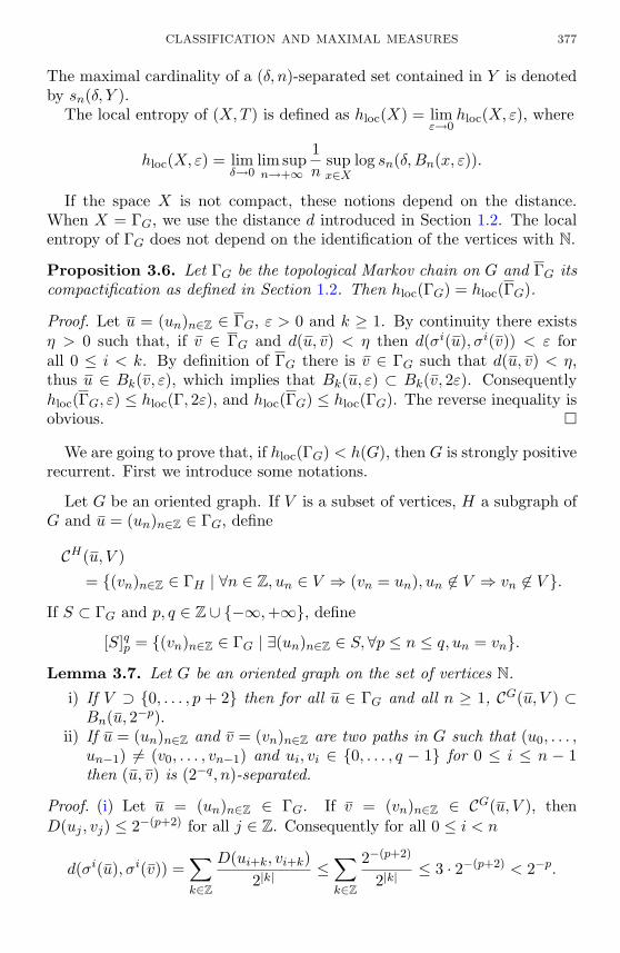
CLASSIFICATION AND MAXIMAL MEASURES 377
The maximal cardinality of a (δ, n)-separated set contained in Y is denotedby sn(δ, Y ).
The local entropy of (X,T ) is defined as hloc(X) = limε→0
hloc(X, ε), where
hloc(X, ε) = limδ→0
lim supn→+∞
1n
supx∈X
log sn(δ,Bn(x, ε)).
If the space X is not compact, these notions depend on the distance.When X = ΓG, we use the distance d introduced in Section 1.2. The localentropy of ΓG does not depend on the identification of the vertices with N.
Proposition 3.6. Let ΓG be the topological Markov chain on G and ΓG itscompactification as defined in Section 1.2. Then hloc(ΓG) = hloc(ΓG).
Proof. Let u = (un)n∈Z ∈ ΓG, ε > 0 and k ≥ 1. By continuity there existsη > 0 such that, if v ∈ ΓG and d(u, v) < η then d(σi(u), σi(v)) < ε forall 0 ≤ i < k. By definition of ΓG there is v ∈ ΓG such that d(u, v) < η,thus u ∈ Bk(v, ε), which implies that Bk(u, ε) ⊂ Bk(v, 2ε). Consequentlyhloc(ΓG, ε) ≤ hloc(Γ, 2ε), and hloc(ΓG) ≤ hloc(ΓG). The reverse inequality isobvious.
We are going to prove that, if hloc(ΓG) < h(G), then G is strongly positiverecurrent. First we introduce some notations.
Let G be an oriented graph. If V is a subset of vertices, H a subgraph ofG and u = (un)n∈Z ∈ ΓG, define
CH(u, V )
= (vn)n∈Z ∈ ΓH | ∀n ∈ Z, un ∈ V ⇒ (vn = un), un 6∈ V ⇒ vn 6∈ V .
If S ⊂ ΓG and p, q ∈ Z ∪ −∞,+∞, define
[S]qp = (vn)n∈Z ∈ ΓG | ∃(un)n∈Z ∈ S,∀p ≤ n ≤ q, un = vn.
Lemma 3.7. Let G be an oriented graph on the set of vertices N.
i) If V ⊃ 0, . . . , p + 2 then for all u ∈ ΓG and all n ≥ 1, CG(u, V ) ⊂Bn(u, 2−p).
ii) If u = (un)n∈Z and v = (vn)n∈Z are two paths in G such that (u0, . . . ,un−1) 6= (v0, . . . , vn−1) and ui, vi ∈ 0, . . . , q − 1 for 0 ≤ i ≤ n − 1then (u, v) is (2−q, n)-separated.
Proof. (i) Let u = (un)n∈Z ∈ ΓG. If v = (vn)n∈Z ∈ CG(u, V ), thenD(uj , vj) ≤ 2−(p+2) for all j ∈ Z. Consequently for all 0 ≤ i < n
d(σi(u), σi(v)) =∑k∈Z
D(ui+k, vi+k)2|k|
≤∑k∈Z
2−(p+2)
2|k|≤ 3 · 2−(p+2) < 2−p.
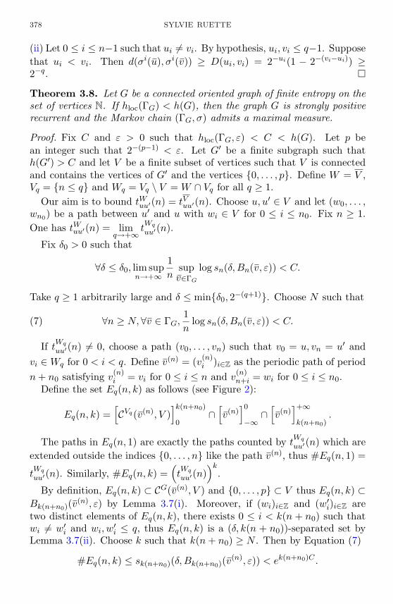
378 SYLVIE RUETTE
(ii) Let 0 ≤ i ≤ n−1 such that ui 6= vi. By hypothesis, ui, vi ≤ q−1. Supposethat ui < vi. Then d(σi(u), σi(v)) ≥ D(ui, vi) = 2−ui(1 − 2−(vi−ui)) ≥2−q.
Theorem 3.8. Let G be a connected oriented graph of finite entropy on theset of vertices N. If hloc(ΓG) < h(G), then the graph G is strongly positiverecurrent and the Markov chain (ΓG, σ) admits a maximal measure.
Proof. Fix C and ε > 0 such that hloc(ΓG, ε) < C < h(G). Let p bean integer such that 2−(p−1) < ε. Let G′ be a finite subgraph such thath(G′) > C and let V be a finite subset of vertices such that V is connectedand contains the vertices of G′ and the vertices 0, . . . , p. Define W = V ,Vq = n ≤ q and Wq = Vq \ V = W ∩ Vq for all q ≥ 1.
Our aim is to bound tWuu′(n) = tVuu′(n). Choose u, u′ ∈ V and let (w0, . . . ,wn0) be a path between u′ and u with wi ∈ V for 0 ≤ i ≤ n0. Fix n ≥ 1.One has tWuu′(n) = lim
q→+∞tWq
uu′(n).
Fix δ0 > 0 such that
∀δ ≤ δ0, lim supn→+∞
1n
supv∈ΓG
log sn(δ,Bn(v, ε)) < C.
Take q ≥ 1 arbitrarily large and δ ≤ minδ0, 2−(q+1). Choose N such that
∀n ≥ N,∀v ∈ ΓG,1n
log sn(δ,Bn(v, ε)) < C.(7)
If tWq
uu′(n) 6= 0, choose a path (v0, . . . , vn) such that v0 = u, vn = u′ andvi ∈Wq for 0 < i < q. Define v(n) = (v(n)
i )i∈Z as the periodic path of periodn+ n0 satisfying v(n)
i = vi for 0 ≤ i ≤ n and v(n)n+i = wi for 0 ≤ i ≤ n0.
Define the set Eq(n, k) as follows (see Figure 2):
Eq(n, k) =[CVq(v(n), V )
]k(n+n0)
0∩[v(n)
]0−∞
∩[v(n)
]+∞k(n+n0)
.
The paths in Eq(n, 1) are exactly the paths counted by tWq
uu′(n) which areextended outside the indices 0, . . . , n like the path v(n), thus #Eq(n, 1) =
tWq
uu′(n). Similarly, #Eq(n, k) =(tWq
uu′(n))k
.
By definition, Eq(n, k) ⊂ CG(v(n), V ) and 0, . . . , p ⊂ V thus Eq(n, k) ⊂Bk(n+n0)(v(n), ε) by Lemma 3.7(i). Moreover, if (wi)i∈Z and (w′i)i∈Z aretwo distinct elements of Eq(n, k), there exists 0 ≤ i < k(n + n0) such thatwi 6= w′i and wi, w
′i ≤ q, thus Eq(n, k) is a (δ, k(n + n0))-separated set by
Lemma 3.7(ii). Choose k such that k(n+ n0) ≥ N . Then by Equation (7)
#Eq(n, k) ≤ sk(n+n0)(δ,Bk(n+n0)(v(n), ε)) < ek(n+n0)C .
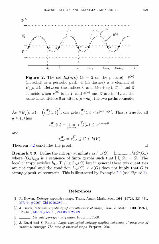
CLASSIFICATION AND MAXIMAL MEASURES 379
NI
-n0
u’u
0 n n+n 2n+n i
(n)vu
Wq
2(n+n 0)
Vu u’u u’
0 0
Figure 2. The set Eq(n, k) (k = 2 on the picture): v(n)
(in solid) is a periodic path, u (in dashes) is a element ofEq(n, k). Between the indices 0 and k(n + n0), v(n) and u
coincide when v(n)i is in V and v(n) and u are in Wq at the
same time. Before 0 or after k(n+n0), the two paths coincide.
As #Eq(n, k) =(tWq
uu′(n))k
, one gets tWq
uu′(n) < e(n+n0)C . This is true for allq ≥ 1, thus
tWuu′(n) = limq→+∞
tWq
uu′(n) ≤ e(n+n0)C
andτWuu′ = τVuv′ ≤ C < h(V ).
Theorem 3.2 concludes the proof.
Remark 3.9. Define the entropy at infinity as h∞(G) = limn→+∞ h(G\Gn)where (Gn)n≥0 is a sequence of finite graphs such that
⋃nGn = G. The
local entropy satisfies hloc(ΓG) ≥ h∞(G) but in general these two quantitiesare not equal and the condition h∞(G) < h(G) does not imply that G isstrongly positive recurrent. This is illustrated by Example 2.9 (see Figure 1).
References
[1] R. Bowen, Entropy-expansive maps, Trans. Amer. Math. Soc., 164 (1972), 323-331,MR 44 #2907, Zbl 0229.28011.
[2] J. Buzzi, Intrinsic ergodicity of smooth interval maps, Israel J. Math., 100 (1997),125-161, MR 99g:58071, Zbl 0889.28009.
[3] , On entropy-expanding maps. Preprint, 2000.
[4] J. Buzzi and S. Ruette, Large topological entropy implies existence of measures ofmaximal entropy: The case of interval maps. Preprint, 2001.

380 SYLVIE RUETTE
[5] M. Denker, C. Grillenberger and K. Sigmund, Ergodic Theory on Compact Spaces,Lecture Notes in Mathematics, 527, Springer-Verlag, 1976, MR 56 #15879,Zbl 0328.28008.
[6] U. Fiebig, Symbolic Dynamics and Locally Compact Markov Shifts, 1996, Habilita-tionsschrift, U. Heidelberg.
[7] B.M. Gurevic, Topological entropy of enumerable Markov chains (Russian), Dokl.Akad. Nauk SSSR, 187 (1969), 715-718; English translation: Soviet Math. Dokl.,10(4) (1969), 911-915, MR 41 #7767, Zbl 0194.49602.
[8] , Shift entropy and Markov measures in the path space of a denumerable graph(Russian), Dokl. Akad. Nauk SSSR, 192 (1970), 963-965; English translation: SovietMath. Dokl., 11(3) (1970), 744-747, MR 42 #3254, Zbl 0217.38101.
[9] B.M. Gurevic and S.V. Savchenko, Thermodynamic formalism for countable sym-bolic Markov chains (Russian), Uspekhi Mat. Nauk, 53(2) (1998), 3-106; Eng-lish translation: Russian Math. Surveys, 53(2) (1998), 245-344, MR 2000c:28028,Zbl 0926.37009.
[10] B.M. Gurevic and A.S. Zargaryan, Existence conditions of a maximal measure fora countable symbolic Markov chain (Russian), Vestnik Moskov. Univ. Ser. I Mat.Mekh., 43(5) (1988), 14-18; English translation: Moscow Univ. Math. Bull., 1988,18-23, MR 91b:58122, Zbl 0717.60083.
[11] S.E. Newhouse, Continuity properties of entropy, Ann. of Math. (2), 129(2) (1989),215-235; Corrections, 131(2) (1990), 409-410, MR 90f:58108, Zbl 0688.58022,Zbl 0693.58009.
[12] W. Parry, Intrinsic Markov chains, Trans. Amer. Math. Soc., 112 (1964), 55-66,MR 28 #4579, Zbl 0127.35301.
[13] I.A. Salama, Topological entropy and recurrence of countable chains, Pacific J. Math.,134(2) (1988), 325-341; Errata, 140(2) (1989), 397, MR 90d:54076, MR 90k:54055,Zbl 0619.54031.
[14] , On the recurrence of countable topological Markov chains, in ‘Symbolic dy-namics and its applications’ (New Haven, CT, 1991), Contemp. Math., 135, 349-360,Amer. Math. Soc., Providence, RI, 1992, MR 93m:54071, Zbl 0801.54032.
[15] O.M. Sarig, Phase transitions for countable Markov shifts, Comm. Math. Phys.,217(3) (2001), 555-577, MR 2002b:37040.
[16] D. Vere-Jones, Geometric ergodicity in denumerable Markov chains, Quart. J. Math.Oxford Ser. (2), 13 (1962), 7-28, MR 25 #4571, Zbl 0104.11805.
Received April 26, 2001 and revised June 20, 2002.
Institut de Mathematiques de LuminyCNRS UPR 9016163 avenue de Luminy, case 90713288 Marseille cedex 9FranceE-mail address: [email protected]

PACIFIC JOURNAL OF MATHEMATICSVol. 209, No. 2, 2003
REMOVABLE SINGULARITIES FOR YANG–MILLSCONNECTIONS IN HIGHER DIMENSIONS
Baozhong Yang
We prove several removable singularity theorems for sin-gular Yang–Mills connections on bundles over Riemannianmanifolds of dimensions greater than four. We obtain thelocal and global removability of singularities for Yang–Millsconnections with L∞ or L
n2 bounds on their curvature ten-
sors, with weaker assumptions in the L∞ case and stronger as-sumptions in the L
n2 case. With the global gauge construction
methods we developed, we also obtain a ‘stability’ result whichasserts that the existence of a connection with uniformly smallcurvature tensor implies that the underlying bundle must beisomorphic to a flat bundle.
1. Introduction.
Uhlenbeck’s original paper [11] on removing isolated singularities of Yang-Mills connections on four manifolds is important not only in its applicationsin the compactification of the moduli space of self-dual connections on Rie-mannian four manifolds, but also in the analytic techniques introduced init. Later on, there has been much work on the removable singularities forYang-Mills connections. Some of these work focused on the case of isolatedsingularities for connections in different dimensions and possibly coupledwith a section (a Higgs field), such as [1], [4], [6] and [7]. Some other workstreated more general singularities, such as [5], [3], [8] and [10]. The fun-damental work of Tian in [10] on the analysis of Yang-Mills connections inhigher dimensions gave some guidance on what we should expect about thesingularities of Yang-Mills connections on manifolds of dimensions greaterthan 4. It turns out that if we are considering connections within the com-pactification of smooth Yang-Mills connections on an n-dimensional mani-fold, then the most general type of singularities to start with is probably anHn−4-rectifiable closed set. While the most general removable singularitytheorem in higher dimensions has not been proved yet, this paper is an effortto understand the removable singularities and the related gauge problemsin higher dimensions.
We shall assume that all the vector bundles in this paper have a compactstructure group G and all connections and gauge transformations refer to
381
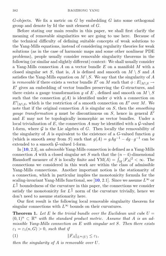
382 BAOZHONG YANG
G-objects. We fix a metric on G by embedding G into some orthogonalgroup and denote by Id the unit element of G.
Before stating our main results in this paper, we shall first clarify themeaning of removable singularities we are going to use here. Because ofthe technical difficulty of defining suitable concepts of weak solutions tothe Yang-Mills equations, instead of considering regularity theories for weaksolutions (as in the case of harmonic maps and some other nonlinear PDEproblems), people usually consider removable singularity theorems in thefollowing (or similar and slightly different) context: We shall usually considera Yang-Mills connection A on a vector bundle E on a manifold M with aclosed singular set S, that is, A is defined and smooth on M \ S and Asatisfies the Yang-Mills equation on M \S. We say that the singularity of Ais removable if there exists a vector bundle E′ on M such that φ : E|M\S →E′ gives an embedding of vector bundles preserving the G-structures, andthere exists a gauge transformation g of E , defined and smooth on M \ Ssuch that the connection g(A) is identified under φ with a connection onE′|M\S , which is the restriction of a smooth connection on E′ over M . Wenote that if the original connection A is singular on S, then the smoothinggauge transformation g must be discontinuous on S, hence in general E′
and E may not be topologically isomorphic as vector bundles. Under alocal trivialization of E, the connection A may be identified with a G-valued1-form, where G is the Lie algebra of G. Then locally the removability ofthe singularity of A is equivalent to the existence of a G-valued function g(which is smooth away from S) such that g(A) = gAg−1 − dg · g−1 can beextended to a smooth G-valued 1-form.
In [10, 2.3], an admissible Yang-Mills connection is defined as a Yang-Millsconnection A with a closed singular set S such that the (n− 4)-dimensionalHausdorff measure of S is locally finite and YM(A) =
∫M |FA|2 < ∞. The
connections we considered in this work are within the class of admissibleYang-Mills connections. Another important notion is the stationarity ofa connection, which in particular implies the monotonicity formula for thescaling-invariant Yang-Mills functional, see [10, 2.1]. Since we assume L∞ orL
n2 boundedness of the curvature in this paper, the connections we consider
satisfy the monotonicity for Ln2 norm of the curvature trivially, hence we
don’t need to assume stationarity here.Our first result is the following local removable singularity theorem for
singular connections with L∞ bounds on their curvatures.
Theorem 1. Let E be the trivial bundle over the Euclidean unit cube U =(0, 1)n ⊂ Rn with the standard product metric. Assume that A is an ad-missible Yang-Mills connection on E with singular set S. Then there existsε1 = ε1(n,G) > 0, such that if
‖FA‖L∞(U) ≤ ε1,(1)
then the singularity of A is removable over U .
REMOVABLE SINGULARITIES 383
We note that there is no extra assumption about the singularity set S ex-cept closedness and the dimensional requirement. With some global gaugepatching arguments, we have the following global version of the above the-orem:
Theorem 2. We assume that M is a compact Riemannian manifold suchthat all representations π1(M) → G are the trivial one and E is the trivialsmooth bundle over M with a smooth G-structure. Assume that A is aYang-Mills connection on E with singularity set S. Then there exists ε2 =ε2(M,G) > 0, such that if
‖FA‖L∞(M) ≤ ε2,(2)
then the singularity of A is globally removable.
We should mention that without the triviality of the bundle E, theremight not be global smoothing gauges for A even if the singularity of A islocally removable (see the remark at the end of Section 4). Our global patch-ing arguments also yield some ‘stability’ results which roughly mean that abundle close to a flat bundle (in some sense) must be flat. In particular, wehave:
Theorem 3 (Corollary 2). Assume that M is a compact n-dimensional Rie-mannian manifold and E is a smooth vector bundle over M with a smoothconnection A on it. Then there exists a constant ε9 = ε9(M) > 0, such thatif
‖FA‖L∞(M) ≤ ε9,(3)
then E is smoothly isomorphic to a flat bundle.
It might be possible to improve the L∞ norm bounds in the above theoremto some Lp (p <∞) bounds. In the next two theorems, we use the L
n2 norm
instead of the L∞ norm of the curvature of the connection. We also assumethe singularity set to be a manifold.
Assume that 4 ≤ k ≤ n is an integer. Let Bk1 be the open unit k-ball in Rk,
and D1 = Bn−k1 ×Bk
1 ⊂ Rn be the Cartesian product of two balls. Assumethat E is a trivial vector bundle on D1 \ (Bn−k
1 × 0). We shall considerconnections with singularity Bn−k
1 × 0 ⊂ D1. This is the standard localmodel for connections with singularities being manifolds of codimension atleast 4.
Theorem 4. Assume that A is a Yang-Mills connection on E with the sin-gularity Bn−k
1 ×0 ⊂ D1. Then there exists a constant ε3 = ε3(n, k,G) > 0,such that if
‖F eA‖Ln2 (D1\(Bn−k
1 ×0) ≤ ε3,(4)
then the singularity of A is removable over D 12
= Bn−k12
×Bn−k12
.

384 BAOZHONG YANG
The following global version is a corollary of Theorem 2 and Theorem 4:
Theorem 5. We assume that M is a compact Riemannian manifold suchthat all representations π1(M) → G are the trivial one and E is the trivialsmooth bundle over M with a smooth G-structure. Assume that A is a Yang-Mills connection on E such that the singularity set S of A is a closed smoothsubmanifold of codimension ≥ 4. Then there exists ε4 = ε4(M,G) > 0, suchthat if
‖FA‖Ln2 (M)
≤ ε4, ∀x ∈M,
then the singularity of A is removable.
We make the assumption that S is a submanifold because we need thegood product local model to prove Theorem 4. It is conceivable that this as-sumption may be relaxed. A conjecture is that we don’t need any additionalassumption on S.
We remark here also that if we allow the constant ε4 in Theorem 5 to de-pend also on the singularity set S, then the conclusion of Theorem 5 followsfrom the local theorem, Theorem 4 directly without the need of Theorem 2.We also would like to point out that a similar result to Theorem 4 for cou-pled Yang-Mills-Higgs fields has been proved in Thomas Otway’s paper [3].Our proof of Theorem 4 here is based on the work of Rado [5] on singu-lar connections on four manifolds with codimension two singularities. Afterwe finished this work, we learned that in a recent work [9], Tao and Tianproved the local removability of singularities for stationary admissible Yang-Mills connections with singularities being manifolds. That will be a strongerresult than Theorem 4 here.
In Section 2 we prove Theorem 4 and Theorem 5. In Section 3 we usesome local gauge patching techniques to prove Theorem 1. In Section 4, wedevelop some global gauge patching results, including Theorem 3 and finallyprove Theorem 2.
2. Removable singularities with Ln2 norm bounds of curvatures.
Assume that 3 ≤ k ≤ n is an integer. Let Bk1 be the open unit k-disk in
Rk, and D1 = Bn−k1 × Bk
1 ⊂ Rn. Assume that E → D1 \ (Bn−k1 × 0) is a
trivial vector bundle.
Theorem 6. There exist constants ε5 = ε5(n, k,G) > 0 and C = C(n, k,G)> 0, such that if ∇+A is a connection on E with the singularity Bn−k
1 ×0,A ∈ L
n21,loc(D1 \ (Bn−k
1 × 0)), and FA ∈ Ln2 (D1), and
‖FA‖Ln2 (D1)
≤ ε5,(5)
REMOVABLE SINGULARITIES 385
then ∇ + A is gauge equivalent, by a gauge transformation in Ln22,loc(D1 \
(Bn−k1 × 0)) to a connection of the form ∇+ A, A ∈ L
n21 (D1), and
‖A‖L
n21 (D1)
≤ C‖FA‖Ln2 (D1)
.
Proof. This theorem is a higher dimensional generalization of Theorem 2.1in Johan Rade [5]. Actually the setting of the theorem in [5] is even morecomplicated because Rade considered the possibility of nontrivial holonomyaround a codimension 2 singularity. Since the codimension of the singularityhere is at least 3, the complement of the singular set, D1 \ (Bn−k
1 × 0),is simply connected and we can follow the proof in [5] omitting the partinvolving holonomy to prove the theorem. Of course, since we are in then-dimensional setting, we need to modify the statements of the lemmas andresults in [5] (stated in 4-dimensional setting there) accordingly. Mainly wejust need to adjust the indices of the various objects and norms. It is nothard to check that the proofs there still work out with these changes andwe shall not reproduce the details here.
Proposition 1. An admissible Yang-Mills connection A on a vector bundleE over M is a weak solution of the Yang-Mills equation, i.e.,
∫M〈dAω, FA〉 = 0,(6)
for any ω ∈ C∞c (M,T ∗M ⊗AdE).
Proof. This type of results are well-known to analysts. For completeness,we give a proof here. Since the question is local, we may assume that Mand the singular set S of A are compact. Assume that Hn−4(M) = m <∞.For any δ > 0, we may find finitely many (geodesic) open balls Bri(xi) ofradii ri < δ, such that xi ∈ S, S ⊂ ∪Bi and
∑rn−4i ≤ Cm. Choose cutoff
functions φi such that φi = 0 on Bri(xi), φi = 1 on M \B2ri(xi), 0 ≤ φi ≤ 1on M and |∇φi| ≤ Cr−1
i on M . Let φ = φδ = infi φi on M . Then φ(x) issupported away from S and if we let N2δ(S) = y ∈ M : dist(y, S) ≤ 2δ,then φ(x) = 1 if x ∈M \N2δS. We have
|∇φ(x)| ≤ supi|∇φi(x)|, ∀x ∈M.
Now we have, for any ω ∈ Ω(AdE),

386 BAOZHONG YANG
∫Mφ〈dAω, FA〉
= −∫Mφ tr(dAω ∧ ∗FA)
= −∫Md(φ tr(ω ∧ ∗FA)) +
∫Mdφ ∧ tr(ω ∧ ∗FA) + (−1)
∫Mφ tr(ω ∧ dA ∗ FA)
=∫Mdφ ∧ tr(ω ∧ ∗FA), because A is smooth Yang-Mills away from S.
Now∣∣∣∣∫Mdφ ∧ tr(ω ∧ ∗FA)
∣∣∣∣ ≤ C
∫M|∇φ||FA|
≤ C
(∫N2δ(S)
|∇φ|2) 1
2(∫
N2δ(S)|FA|2
) 12
≤ C
(∑i
∫N2δ(S)
|∇φi|2) 1
2(∫
N2δ(S)|FA|2
) 12
= C
(∑i
∫B2ri
(xi)|∇φi|2
) 12(∫
N2δ(S)|FA|2
) 12
≤ C
(∑i
rn−2i
)(∫N2δ(S)
|FA|2) 1
2
≤ C
(∫N2δ(S)
|FA|2) 1
2
.
If we let δ → 0, then the last right-hand side goes to 0 by the L2 integrabilityof FA. On the other hand∫
Mφδ〈dAω, FA〉 →
∫M〈dAω, FA〉.
This gives the weak Equation (6).
Remark. We note here that if A ∈ Ln21 and A satisfies the Yang-Mills
equation weakly, then for any gauge transformation g ∈ Ln22 , g(A) = gAg−1−
dgg−1 is still a weak solution of the Yang-Mills equation. The reason isas follows: We have d∗g(A)Fg(A) = g(d∗AFA)g−1. By Sobolev embedding
theorems, g, g−1 ∈ Ln22 and d∗AFA = 0 in L
n2−1 imply that g(d∗AFA)g−1 is
REMOVABLE SINGULARITIES 387
well-defined in Lp−1, for any p < n2 . Hence d∗g(A)Fg(A) = 0 in Lp−1. That
implies g(A) satisfies the Yang-Mills equation weakly.
Now we are ready to prove Theorem 4 — the ε-regularity theorem foradmissible Yang-Mills connections with L
n2 bounds on the curvature.
Proof of Theorem 4. Assume that ε3 < ε5. Then the connection satisfies theassumption of Theorem 6. We first apply Theorem 6 to the given connectionto obtain a L
n22 gauge in which the connection, still denoted A, is in L
n21 .
Now we may apply the existence theorem of Hodge gauges, Theorem 1.3 inUhlenleck [12] to see that if ε3 is sufficiently small, then after a further L
n22
gauge transformation, we can make the resulting connection, again denotedA, to be in the Hodge gauge, i.e.,
d∗A = 0,(7)
and with the following elliptic boundary condition:
∗A = 0, on ∂D1.(8)
Since the original admissible Yang-Mills connection is a weak solution of theYang-Mills equation by Prop. 1, and the gauges we have used are all in L
n22 ,
it follows from the previous remark that we have the weak equation,
d∗AFA = 0.(9)
Now (7), (8) and (9) form a uniform elliptic system with A ∈ Ln21 (D1).
Therefore, by standard elliptic theory, we may obtain higher regularitiesand the smoothness of A in D1. This removes the singularity.
Proof of Theorem 5. If ε4 is sufficiently small, then the assumptions of The-orem 4 are satisfied locally and we have that locally the singularity of A isremovable. Since |FA| is gauge-invariant, we have in particular that |FA|2 isa smooth function on M . However, |FA|2 satisfies a Bochner-Weitzenbockformula and hence the following a priori estimates (by Uhlenbeck, see also[2]):
|FA|2(x) ≤ C
(ρ−n
∫Bρ(x)
|FA|n2 dv
) 4n
, ∀x ∈M.(10)
We remark here that although the a priori estimates are usually stated forsmooth (or stationary) Yang-Mills connections and for scaling invariant L2
energies ρ4−n ∫Bρ(x) |FA|
2dv, we have here the bounds on the Ln2 energy
which is itself scaling invariant. Corresponding to the monotonicity formulaused in the proof of the usual a priori estimates, we have trivially that∫
Bρ(x)|FA|
n2 dv ≤
∫Bσ(x)
|FA|n2 dv, if ρ ≤ σ.

388 BAOZHONG YANG
Hence the proof of the usual a priori estimates (see [2] or [10, 2.2.1]) can beadapted (almost word by word) to give our version (10). We shall not givethe details and refer the reader to the references.
By (10), if ε4 is small enough, we have
‖FA‖L∞(M) ≤ ε2,
and hence Theorem 2 applies to give the global removability of the singu-larity of A.
3. Removable singularities with L∞ norm bounds of curvatures.
The essence of the Proof of Theorem 1 is a construction of a smoothinggauge transformation. The method we shall use here is a refinement ofUhlenbeck’s method to construct global gauges on compact manifolds usedin §3 of [12]. The idea of this argument is to modify and glue suitable gaugeson different patches inductively to obtain a global gauge. Here because wehave infinitely many patches, we have to keep a careful track of the gluingprocedure to make sure the gauges we obtained are always suitably bounded,thus amenable for further gluing in the induction.
Before giving the proofs, we introduce the following definitions to makethe statements simpler. Let M be a Riemannian manifold and let the indexset I be either the set of natural numbers or the set 1, 2, . . . , n for someinteger n.
Definition. Let c > 0 be a constant and K > 0 be an integer. We call acountable collection of open subsets of M , U iαα∈I,1≤i≤K , a (c,K)-uniformnested covering of M if the following conditions are satisfied:
1) U i+1α ⊂ U iα, for 1 ≤ i ≤ K − 1.
2) M ⊂⋃α∈I U
Kα .
3) #α : x ∈ U1α ≤ K, ∀x ∈M .
4) The diameters rα = diam(U1α) satisfy,
rα ≤ crβ , if U1α ∩ U1
β 6= ∅.
This definition of nested open sets is natural because we shall see that inthe gluing procedure, we need to shrink the open sets each time we try to gluegauges on overlapping open patches. Let U iαα∈I,1≤i≤K be a (c,K)-uniformcovering of M . We shall define integers iαβ for all pairs (α, β) satisfyingα ≥ β. First we define for any α ∈ I, iαα = 1. Then we define inductivelyfor α > β that
iαβ =
iα−1β + 1, if U
iα−1β
β ∩ U1α 6= ∅,
iα−1β , otherwise.
(11)

REMOVABLE SINGULARITIES 389
Note that because of 3) in the definition, for any α ∈ I, 1 = iαα ≤ iα+1α ≤
· · · ≤ K, and the increasing sequence stabilizes to an integer, which we willdenote by iα.
Definition. We call a (c,K)-uniform nested covering U iαα∈I,1≤i≤K of Ma good (c,K)-uniform nested covering if there exist functions ψα ∈ C∞(U1
α)such that for each α ∈ I,
ψα ≡ 1, on U1α ∩
⋃β<α
Uiαββ
,(12)
ψα ≡ 0, on U1α \
⋃β<α
Uiα−1β
β
,(13)
0 ≤ ψα ≤ 1, rα|∇ψα| ≤ c, on U1α, where rα = diam(U1
α).(14)
We recall that a collection of transition functions gαβ with respect toan open covering Uα of M consist of functions gαβ : Uα ∩ Uβ → G onUα ∩ Uβ 6= ∅ such that:
1) gαβgβα = Id, on Uα ∩ Uβ,2) gαβgβγgγα = Id, on Uα ∩ Uβ ∩ Uγ .
Definition. We call a collection of transition functions gαβ ∈ C1(Uα ∩Uβ, G) a collection of δ-small transition functions with respect to a coveringUαα∈I with length scales rαα∈I if, setting rα = diam(Uα), we have
|gαβ − Id |+ rα|∇gαβ | ≤ δrα, on Uα ∩ Uβ.(15)
The above technical definitions will enable us to track the bounds effec-tively in the gluing procedure.
Lemma 1. For any c0 > 0 and K a positive integer, there exists δ0 =δ0(c0,K,diam(M), G) > 0 such that if δ < δ0, U iαα∈I,1≤i≤K is a good(c0,K)-uniform nested covering of M and gαβ is a collection of δ-smalltransition functions with respect to the covering U1
αα∈I , then there exist acollection of functions hα ∈ C1(U1
α, G) and a constant C = C(c0, n,K,G) >0 such that
gαβ = h−1α hβ , on U iαα ∩ U iββ ,(16)
|hα − Id |+ rα|∇hα| ≤ Cδrα, on U1α.(17)
Proof. For simplicity, we use Uα to denote U1α in the proof. We shall prove
by induction on α ∈ I that there exist hα ∈ C1(Uα, G) and constants C(k) =C(k, n, c0, G) > 0 for 1 ≤ k ≤ K such that for any α ∈ I,
gβγ = h−1β hγ , on U
iαββ ∩ U i
αγγ , β, γ ≤ α,(18)
|hα(x)− Id |+ rα|∇hα(x)| ≤ C(lαx )δ, ∀x ∈ Uα,(19)
390 BAOZHONG YANG
where lαx = #β ≤ α : x ∈ Uβ ≤ K. We note that if (18) and (19) holdfor all α ∈ I, then by taking C = max1≤k≤K C(k), (16) and (17) will followimmediately.
Let α0 be the smallest element of I, we define hα0(x) = Id ∈ G forx ∈ Uα0 . Then (18) and (19) are trivially satisfied for α = α0 (for any valueof C(1) > 0). Now suppose that we have defined hβ ∈ C1(Uβ, G) for allβ < α such that (18) and (19) hold for indices < α.
We define
hα(x) = exp(ψα(x) exp−1(hβ(x)gβα(x))), ∀x ∈ Uα ∩ Uiα−1β
β ,∀β < α,(20)
hα(x) = Id, ∀x ∈ Uα \
⋃β<α
Uiα−1β
β
.(21)
We note that by the induction hypothesis, if β < α, then |hβ(x)gβα(x)−Id | ≤ Cδrβ ≤ Cδ and |φα(x)| ≤ 1 by (14). Hence if δ is sufficiently small,then the expression in (20) involving exp and exp−1 in (20) is meaningful.The definition in (20) is unambiguous for different choices of β because ofthe induction hypothesis (18) for indices β, γ < α and the assumption thatgαβ are transition functions. We note that the definition (20) and (21)determine a well-defined hα ∈ C1(Uα, G) because of (12) and (13). It followseasily by (12) and (20), and the fact that gβγ are transition functions that(18) holds for all β, γ ≤ α.
If x ∈ Uα ∩ Uiα−1β
β with β < α, then by (14), (15), (20), (21) and theinduction hypothesis, there exists a constant C1 = C1(n, c0) > 0, such that,
|hα(x)− Id | ≤ C1|hβ(x)gβα(x)− Id | ≤ C1(1 + C(lα−1))δrα,
rα|∇hα(x)| ≤ C1rα(|∇ψα(x)||hβ(x)gβα(x)− Id |+ |∇hβ(x)|+ |∇gβα(x)|)≤ C1(1 + C(lα−1
x ))δrα.
It follows that if at the beginning we define C(1) = C1 and inductively defineC(k + 1) = C1(1 + C(k)) (these definitions only depend on n, K and c0),then (19) will be true for α. This finishes the induction step and the proofof the lemma.
Proof of Theorem 1. We shall choose a collection F of disjoint open dyadiccubes in U\S step by step in the following way (the Whitney decomposition):At the first step, we divide U into 2n congruent disjoint open cubes withedges of length 1/2. For k ≥ 2, in the k-th step, we consider dyadic cubeswith edges of length 1/2k−1 which (or a cube containing it) have not been putin F in the previous steps; if such a cube C satisfies the following condition:
dist(C,S) ≥ diam(C),

REMOVABLE SINGULARITIES 391
then we put C in the collection F ; otherwise, we subdivide C into 2n con-gruent disjoint smaller open cubes with edges of length 1/2k. It is easy tosee that we obtain a collection of disjoint open cubes F = Cα : α ∈ I thisway and we have
U ∩⋃α∈I
Cα = U \ S.
We then let
F =Uα =
(98Cα
)∩ U : α ∈ I
,
where 98Cα is the dilation of Cα at the center of Cα with a factor 9
8 . Thecollection F = Uαα∈I of open sets now satisfies:
1)⋃α∈I Uα = U \ S.
2) If Uα ∈ F , then dist(Uα, S) ≥ 12 diam(Uα).
3) If Uα, Uβ ∈ F , and Uα ∩ Uβ 6= ∅, then diamUβ ≤ 3 diam(Uα).4) There exists a number K = K(n), such that #α : x ∈ Uα ∈ F ≤ K.
Let λ(i) = exp(K+1−iK log 9
8) for 1 ≤ i ≤ K and define U iα = λ(i)Cα∩U forα ∈ I and 1 ≤ i ≤ K. We note that U1
α = Uα and Cα ⊂ UKα , U i+1α ⊂ U iα for
1 ≤ i ≤ K−1. It is then easy to check that there exists a constant c0 = c0(n)such that U iαα∈I,1≤i≤K is a good (c0,K)-uniform nested covering.
Under the trivialization of the bundle on U , the connection may be identi-fied as a matrix valued 1-form A and a gauge transformation can be viewedsimply as a function from U to G. We fix a point x0 ∈ U \ S. Let xα bethe center of the cube Cα. For any point x ∈ Uα, we let γxα be the shortestgeodesic from xα to x inside Uα and define µα(x) ∈ G to be the paralleltransport of the bundle from xα to x along γxα, using the trivialization ofthe bundle.
Note that µα(xα) = Id. We regard µ−1α as gauge transformations on
Uα, and denote µ−1α (A) by Aα. We use the normal spherical coordinates
r, θii=1,...,n−1 centered at xα, where r is the distance to xα. Assume that
Aα = Aα,rdr + Aα,idθi, on Uα
and
F eAα= Fα,ridr ∧ dθi + Fα,ijdθ
i ∧ dθj , on Uα.
Then by the definition of µα, we have Aα,r ≡ 0 on Uα. Hence
∂r(Aα,i) = Fα,ri, i = 1, . . . , n− 1.(22)

392 BAOZHONG YANG
By integrating (22) and using that Aα(0) = 0, we have
|Aα|(x) ≤ C|x| ·∫ 1
0|F eAα
|(tx)dt(23)
= C|x|∫ 1
0|FA|(tx)dt ≤ C|x|ε1 ≤ Cε1rα.
Remark. The above gauge coming from the parallel transport along a ge-odesic leading from a central point was introduced by Uhlenbeck in [11]. Itmay be called the radially flat gauge at xα. Properties (22) and (23) werealso given in [11].
Since dimS < n− 2, we may perturb the geodesic from xα to x0 slightlyto be disjoint from S and denote the perturbed curve by lα. We defineσα(0) ∈ G to be the parallel transport of the bundle from x0 to xα alongthe curve lα and let
σα(x) = µα(x)σα(0), ∀x ∈ Uα.
If Uα ∩Uβ 6= ∅, we denote the difference between the gauge transformationsσα and σβ by
gαβ = σ−1α σβ = σ−1
a (0)µ−1α (x)µβ(x)σβ(0).(24)
Now assume that x ∈ Uα ∩ Uβ. Consider the closed curve
γ = l−1α (γxα)−1γxβ lβ .
We notice that gαβ(x) ∈ G represents the parallel transport of the bundlealong the closed curve γ. Because dim(S) < n − 2, by perturbation, thereexists a triangle ∆ spanning γ with Area(∆) ≤ crα for some constant c =c(n) and ∆ ∩ S = ∅. By a well-known relation between holonomy andcurvature, we have
|gαβ(x)− Id | ≤∫
∆|FAα(y)|dy ≤ crαε1.(25)
Now we use σα as gauge transformations on Uα and define
Aα = σ−1α (A) = σα(0)−1(Aα) = σα(0)−1 Aα σα(0).
Then (23) and the compactness of G imply that
|Aα|(x) ≤ Cε1rα, ∀x ∈ Uα.(26)
We have by the definition of gαβ that
dgαβ = gαβAβ −Aαgαβ .(27)
It follows from (26) and (27) that
|∇gαβ(x)| ≤ Cε1rα.(28)

REMOVABLE SINGULARITIES 393
Given any δ > 0, if we take ε1 = δ/C, then (25) and (28) imply that gαβis a δ-small collection of transition functions with respect to the coveringUα of U \ S with length scales rα. Therefore Lemma 1 applies andgives the correction term hα on each Uα. Let Vα = U iαα . The new gaugesρα = hασ
−1α on Vα given by the correction of hα now satisfy ρα = ρβ on
Vα ∩ Vβ (because of (16) and (24)). Hence the ρα’s define a global gauge ρon U \ S. We have
|ρ(A)(x)| = |hα(Aα(x))| = |hαAαh−1α − dhα h
−1α |(29)
≤ C(|Aα|+ |∇hα|) ≤ Cε1, ∀x ∈ Vα.
By inspecting our gluing procedure, we know that we can actually requireρ(A) to be smooth away from S, which implies that ρ(A) is admissible anda weak solution of the Yang-Mills equation. (29) and the assumption that‖FA‖ ≤ ε1 implies that
‖A‖Lp1≤ Cε1, ∀p ≤ ∞
because FA = dA+A∧A. Fix n2 < p <∞, if ε1 is sufficiently small, we may
apply the implicit function theorem (see Theorem 2.7 in [11]) to obtainan Lp2 gauge transformation g on U so that the connection A′ = g(ρ(A))satisfies
d∗A′ = 0, on U, ∗A′ = 0, on ∂U(30)
(as (7) and (8) in Theorem 4’s proof). In the new gauge, we have A′ ∈ Lp1.A′ is also the weak solution of
d∗A′FA′ = 0, on U,
by the remark following the proof of Proposition 1. Therefore we obtain thesmoothness of the connection by elliptic regularity and finishes the proof ofthe theorem.
4. Global removable singularity theorems.
Before we carry out the Proof of Theorem 2, we shall first prove the followingtheorem, which is also of independent interest:
Theorem 7. Assume that M is a compact n-dimensional manifold. LetU = Uαα∈I be a finite open covering of M and gαβ, gαβ : Uαβ = Uα ∩Uβ → G, be a set of smooth transition functions with respect to U . Thenthere exist constants ε6 = ε6(M,U) > 0 and C = C(M,U) > 0, such that if
supx,y∈Uαβ
α,β∈I
|gαβ(x)− gαβ(y)| = δ ≤ ε6,(31)

394 BAOZHONG YANG
then there exist a collection of constant transition functions g0αβ, a smaller
covering V = Vα of M , with Vα ⊂ Uα and M ⊂ ∪V, and a set of smoothfunctions ρα : Vα → G, such that
ραgαβρ−1β = g0
αβ , on Vα ∩ Vβ(32)
and
supx∈Vαα∈I
|ρα(x)− Id | ≤ Cδ.(33)
In particular, the bundle defined by gαβ is isomorphic to a flat bundle(defined by g0
αβ).
Proof. We first claim that there exists an increasing continuous functionµ : [0,∞) → [0,∞) with µ(0) = 0, depending only on M and U , such thatif δ is defined by the left-hand side of (31), then there exists a collection ofconstant transition functions g0
αβ with respect to the covering U such that
supx∈Uα∩Uβ
α,β∈I
|gαβ − g0αβ(x)| ≤ µ(δ).(34)
We let J = (α, β)|α < β ∈ I, Uα∩Uβ 6= ∅ and K = (α, β, γ)|α < β < γ ∈I, Uα ∩ Uβ ∩ Uγ 6= ∅. Denote by GJ be the Cartesian product of |J | copiesof G indexed by J , with a general element a = (aαβ), (α, β) ∈ J . Define GK
similarly. We then define a map Φ : GJ → GK by
Φ((aαβ)) = (aαβaβγa−1αγ ) ∈ GK , for any a = (aαβ) ∈ GJ .
Φ is clearly a continuous map. We note that an element a = (aαβ) of GK
gives a collection of constant transition functions with respect to U if andonly if Φ(a) = (Id, . . . , Id) := 1 ∈ GK , i.e., if and only if a ∈ Φ−1(1).Assume that there doesn’t exist such a function µ as claimed above, thenthere exists ε > 0, a sequence δi decreasing to 0 and a sequence of sets oftransition functions giαβ with respect to U , such that
supx,y∈Uαβ
α,β∈I
|giαβ(x)− giαβ(y)| = δi,(35)
and
supx∈Uα∩Uβ
α,β∈I
|giαβ(x)− aαβ | ≥ ε, ∀(aαβ) ∈ Φ−1(1), ∀i.(36)
We fix points xαβ ∈ Uα ∩ Uβ. Because GJ is compact, we know that thesequence (giαβ(xαβ)) ∈ GJ contains a subsequence converging to an element(g0αβ) ∈ GJ . Now the fact that giαβ are sets of transition functions imply

REMOVABLE SINGULARITIES 395
that g0αβ is also a set of transition functions with respect to U , i.e., (g0
αβ) ∈Φ−1(1). The fact that giαβ(xαβ) → g0
αβ together with (35) imply that
supx∈Uα∩Uβ
α,β∈I
|giαβ(x)− g0αβ | → 0, as i→∞.
This clearly contradicts (36) when i. Thus the claim is verified.Now we recall the following proposition by Uhlenbeck (Prop. 3.2 in [12]):
Proposition 2. Let gαβ and hαβ be two sets of smooth transition func-tions with respect to a covering U = Uαα∈I of a compact manifold M .There exist constants ε7 = ε7(M,U) > 0 and C = C(M,U) > 0, such that if
supx∈Uα∩Uβ
α,β∈I
|gαβ(x)− hαβ(x)| ≤ ε7,(37)
then there exists a smaller covering V = Vα of M , with Vα ⊂ Uα andM ⊂ ∪V, and a set of smooth functions ρα : Vα → G, such that
ραgαβρ−1β = hαβ , on Vα ∩ Vβ(38)
and
supx∈Vαα∈I
|ρα(x)− Id | ≤ Cδ.(39)
In particular, the bundle defined by gαβ is smoothly isomorphic to thebundle defined by hαβ.
We apply Proposition 2 to gαβ and g0αβ (found by the claim) and
immediately see that the theorem holds.
There are some corollaries of Theorem 7 in the following:
Corollary 1. Assume that M is a compact Riemannian n-dimensional ma-nifold. Let U = Uαα∈I be a finite open covering of M such that any twopoints x, y in a nonempty intersection Uα ∩ Uβ can be connected by a C1
curve within Uα ∩ Uβ with length ≤ l, a uniform constant, and let gαβbe a set of smooth transition functions with respect to U . Then there existconstants ε8 = ε8(M, l,U) > 0 and C = C(M,U) > 0, such that if
supx∈Uαβ
α,β∈I
|∇gαβ(x)| = δ ≤ ε8,(40)
then we have the same conclusions as in Theorem 7. In particular, thebundle defined by gαβ is smoothly isomorphic to a flat bundle.
Proof. We may easily deduce from (40) and the assumptions that the in-equality (31) holds if we take ε8 = ε6/l. Then we can apply Theorem 7here.

396 BAOZHONG YANG
Corollary 2. Assume that M is a compact n-dimensional Riemannian ma-nifold and E is a smooth vector bundle over M with a smooth connection Aon it. Then there exists ε9 = ε9(M) > 0, such that if
‖FA‖L∞(M) ≤ ε9,(41)
then E is smoothly isomorphic to a flat bundle.
Proof. We cover M with coordinate balls Uα, such that any two pointsx, y in a nonempty intersection Uα ∩ Uβ can be connected by a C1 curvewithin Uα ∩ Uβ with length ≤ diam(M). Let φα : E|Uα → B1(0) × Rl betrivializations on Uα and Aα be the G-valued 1-form on Uα correspondingto A under φα. We use the radially flat gauge of A on Uα, i.e., we findhα : Uα → G such that hα(Aα)(0) = 0 and hα(∂r) = 0 under the localcoordinates Uα ∼= B1(0) ⊂ Rn. We have from (23) that
|hα(Aα)(x)| ≤ C||FA||L∞(M) ≤ Cε9, ∀x ∈ Uα.(42)
We define hαβ = hαφαφ−1β h−1
β on Uα ∩Uβ and we can check that hαβ is aset of transition functions. Now we have
dhαβ = hα(Aα) hαβ − hαβ (hβ(Aα))
and hence from (42), we have
|∇hαβ | ≤ Cε9, on Uα ∩ Uβ .
Now by taking ε9 sufficiently small we may apply Corollary 1 to establishthe theorem.
Proof of Theorem 2. We choose a covering U = Uα of M such that eachUα is a coordinate cube and the metrics of E and M on Uα can be uniformlycompared with the product metric and the Euclidean metric. We also requirethat any two points x, y in a nonempty intersection Uα∩Uβ can be connectedby a C1 curve within Uα ∩Uβ with length ≤ diam(M). If ε2 is taken small,we can now apply Theorem 1 for the connection A on each Uα to obtainlocal gauge transformations hα : Uα → G such that hα(A) are smooth onUα and furthermore, from the Proof of Theorem 1, we may require that
|hα(A)| ≤ C‖FA‖L∞(M) ≤ Cε2,
for some uniform constant C. Now we define hαβ = hαh−1β . hαβ must
be smooth because it intertwines smooth connections hα(A) and hβ(A) onUα ∩Uβ . We can then follow the lines of the last part in the proof of Cor. 2to establish that there exist a refinement V = Vα of the covering U , acollection of smooth functions ρα : Vα → G and a collection of constanttransition functions g0
αβ such that
ραhαβρ−1β = g0
αβ , on Uα ∩ Uβ .

REMOVABLE SINGULARITIES 397
Because every representation of π1(M) → G is the trivial one, every flatbundle over M is trivial. Hence there exists constants λα ∈ G such thatg0αβ = λ−1
α λβ for any α, β. It follows that
λαραhα = λβρβhβ, on Uα ∩ Uβ .Hence we may define a global gauge transformation g by letting g = λαραhα,on Uα. g(A) is smooth on M and hence g gives the desired smoothinggauge.
Remark. We remark that in Theorem 2 if the original bundle E is not triv-ial, then although locally the singularity of the connection A is removable,there may not exist a global gauge transformation which makes A smoothon M . The following is a simple example of this lack of global smoothinggauge. In fact, this example has something to do with the lack of globalsmooth gauge transformations on certain bundles. Let M = S2 = CP 1 withthe covering given by U1 = z : z ∈ C and U2 = w : w ∈ C with thecoordinate change given by z = 1/w on U12 = U1 ∩U2. We give a transitionfunction for a line bundle g12 : U12 → C∗ via
g12(z) =z
|z|∈ C∗.
Let E be the smooth line bundle determined by g12. It is easy to see thatE has the same smooth structure as the hyperplane bundle on P1. We thendefine a connection A on E by letting its local forms be A1 = −idθ on U1
and A2 = 0 on U2, where θ is the usual angle coordinate on C. We cancheck that g12(A1) = A2 and hence A is a well-defined connection on Ewith singularity p = z = 0 ∈ U1. This singularity of A can be removedon U1 as follows. We define ρ : U1 → C by ρ(z) = z/|z|. Then ρ(A1) = 0gives the smoothing of A1 on U1. However, it is clear from homotopicalconsiderations that ρ cannot be extended to a global gauge transformationsmooth on M − p.
We may similarly construct an example of a nontrivial SU(2) bundle onS4 with a flat connection A which is singular at one point but does not havea global smoothing gauge. We note that in these examples the bundles don’tallow global smooth gauge transformations.
Acknowledgment. The author would like to thank Rick Schoen and GangTian for many helpful discussions on this work and the referee for manyuseful suggestions on the revision of this paper.
References
[1] H. Nakajima, Removable singularities for Yang-Mills connections in higher dimen-sions, J. Fac. Sci. Univ. Tokyo Sect. IA Math., 34(2) (1987), 299-307, MR 89d:58029,Zbl 0637.58026.

398 BAOZHONG YANG
[2] , Compactness of the moduli space of Yang-Mills connections in higher dimen-sions, J. Math. Soc. Japan, 40 (1988), MR 89g:58050, Zbl 0647.53030.
[3] T.H. Otway, Higher-order singularities in coupled Yang-Mills-Higgs fields, NonlinearAnal., 15(3) (1990), 239-244, MR 91j:58044, Zbl 0714.58049.
[4] T. Parker, Gauge theories on four-dimensional Riemannian manifolds, Comm. Math.Phys., 85(4) (1982), 563-602, MR 84b:58036, Zbl 0502.53022.
[5] J. Rade, Singular Yang-Mills fields, local theory, II, J. Reine Angew. Math., 456(1994), 197-219, MR 95j:58031, Zbl 0830.53024.
[6] L.M. Sibner, The isolated point singularity problem for the coupled Yang-Mills equa-tions in higher dimensions, Math. Ann., 271(1) (1985), 125-131, MR 86g:58038,Zbl 0558.35073.
[7] , Removable singularities of Yang-Mills fields in R3, Compositio Math., 53(1)(1984), 91-104, MR 86c:58151, Zbl 0552.58037.
[8] L.M. Sibner and R.J. Sibner, Classification of singular Sobolev connections bytheir holonomy, Comm. Math. Phys., 144(2) (1992), 337-350, MR 93a:58042,Zbl 0747.53024.
[9] T. Tao and G. Tian, A singualarity removal theorem for Yang-Mills fields in higherdimensions. Preprint.
[10] G. Tian, Gauge theory and calibrated geometry, I, Ann. of Math. (2), 151(1) (2000),193-268, MR 2000m:53074, Zbl 0957.58013.
[11] K.K. Uhlenbeck, Removable singularities in Yang-Mills fields, Comm. Math. Phys.,83(1) (1982), 11-29, MR 83e:53034, Zbl 0491.58032.
[12] , Connections with Lp bounds on curvature, Comm. Math. Phys., 83(1) (1982),31-42, MR 83e:53035, Zbl 0499.58019.
Received November 27, 2001 and revised May 19, 2002. Research partially supported byNSF Grant DMS-0104163.
Department of MathematicsStanford UniversityStanford, CA 94305E-mail address: [email protected]
CONTENTS
Volume 209, no. 1 and no. 2
Gregory Berhuy, Marina Monsurro and Jean-Pierre Tignol: The discriminant of asymplectic involution 201
M.B. Branco with J.C. Rosales 131
James Conant: Fusion and fission in graph complexes 219
Brian Curtin: Some planar algebras related to graphs 231
H.R. Dowson, M.B. Ghaemi and P.G. Spain: Boolean algebras of projections andalgebras of spectral operators 1
B. Felzenszwalb, A. Giambruno and G. Leal: On rings which are sums of twoPI-subrings: a combinatorial approach 17
Ciprian Foias, Il Bong Jung, Eungil Ko and Carl Pearcy: Complete contractivity ofmaps associated with the Aluthge and Duggal transforms 249
Etienne Fouvry and Philippe Michel: Sommes de modules de sommesd’exponentielles 261
Glenn J. Fox: A method of Washington applied to the derivation of a two-variablep-adic L-function 31
M.B. Ghaemi with H.R. Dowson and P.G. Spain 1
A. Giambruno with B. Felzenszwalb and G. Leal 17
David Helm and Ezra Miller: Bass numbers of semigroup-graded local cohomology 41
James A. Hoffman and Daniel Matignon: Examples of bireducible Dehn fillings 67
Jerzy Jezierski and Wacław Marzantowicz: Homotopy minimal periods for maps ofthree dimensional nilmanifolds 85
Il Bong Jung with Ciprian Foias, Eungil Ko and Carl Pearcy 249
Young-One Kim, Jungseob Lee and Kyewon K. Park: A zeta function for flip systems 289
Eungil Ko with Ciprian Foias, Il Bong Jung and Carl Pearcy 249
G. Leal with B. Felzenszwalb and A. Giambruno 17
Jungseob Lee with Young-One Kim and Kyewon K. Park 289
Andrei K. Lerner: On some pointwise inequalities concerning tent spaces and sharpmaximal functions 303

400
Zhi-Guo Liu: Some Eisenstein series identities related to modular equations of theseventh order 103
Charles Livingston: Observations on Lickorish knotting of contractible 4-manifolds 319
Harald Löwe: Sixteen-dimensional locally compact translation planes admittingSL2H as a group of collineations 325
Wacław Marzantowicz with Jerzy Jezierski 85
Daniel Matignon with James A. Hoffman 67
Philippe Michel with Etienne Fouvry 261
Ezra Miller with David Helm 41
Marina Monsurrò with Gregory Berhuy and Jean-Pierre Tignol 201
Matthew Neal and Bernard Russo: Operator space characterizations of C*-algebrasand ternary rings 339
Kyewon K. Park with Young-One Kim and Jungseob Lee 289
Carl Pearcy with Ciprian Foias, Il Bong Jung and Eungil Ko 249
J.C. Rosales and M.B. Branco: Irreducible numerical semigroups 131
Sylvie Ruette: On the Vere–Jones classification and existence of maximal measuresfor countable topological Markov chains 365
Bernard Russo with Matthew Neal 339
P.G. Spain with H.R. Dowson and M.B. Ghaemi 1
Michael Taylor: The Schrödinger equation on spheres 145
Jean-Pierre Tignol with Gregory Berhuy and Marina Monsurro 201
Cynthia E. Will: The Meromorphic continuation of the resolvent of the Laplacian online bundles over CH(n) 157
Baozhong Yang: Removable singularities for Yang–Mills connections in higherdimensions 381
Fuliu Zhu: The heat kernel and the Riesz transforms on the quaternionic Heisenberggroups 175

Guidelines for Authors
Authors may submit manuscripts at pjm.math.berkeley.edu/about/journal/submissions.htmland choose an editor at that time. Exceptionally, a paper may be submitted in hard copy toone of the editors; authors should keep a copy.
By submitting a manuscript you assert that it is original and is not under considerationfor publication elsewhere. Instructions on manuscript preparation are provided below. Forfurther information, visit the web address above or write to [email protected] orto Pacific Journal of Mathematics, University of California, Los Angeles, CA 90095–1555.Correspondence by email is requested for convenience and speed.
Manuscripts must be in English, French or German. A brief abstract of about 150 words orless in English must be included. The abstract should be self-contained and not make anyreference to the bibliography. Also required are keywords and subject classification for thearticle, and, for each author, postal address, affiliation (if appropriate) and email address ifavailable. A home-page URL is optional.
Authors are encouraged to use LATEX, but papers in other varieties of TEX, and exceptionallyin other formats, are acceptable. At submission time only a PDF file is required; followthe instructions at the web address above. Carefully preserve all relevant files, such asLATEX sources and individual files for each figure; you will be asked to submit them uponacceptance of the paper.
Bibliographical references should be listed alphabetically at the end of the paper. Allreferences in the bibliography should be cited in the text. Use of BibTEX is preferred butnot required. Any bibliographical citation style may be used but tags will be converted tothe house format (see a current issue for examples).
Figures, whether prepared electronically or hand-drawn, must be of publication quality.Figures prepared electronically should be submitted in Encapsulated PostScript (EPS) orin a form that can be converted to EPS, such as GnuPlot, Maple or Mathematica. Manydrawing tools such as Adobe Illustrator and Aldus FreeHand can produce EPS output.Figures containing bitmaps should be generated at the highest possible resolution. If thereis doubt whether a particular figure is in an acceptable format, the authors should checkwith production by sending an email to [email protected].
Each figure should be captioned and numbered, so that it can float. Small figures occupyingno more than three lines of vertical space can be kept in the text (“the curve looks likethis:”). It is acceptable to submit a manuscript will all figures at the end, if their placementis specified in the text by means of comments such as “Place Figure 1 here”. The sameconsiderations apply to tables, which should be used sparingly.
Forced line breaks or page breaks should not be inserted in the document. There is no pointin your trying to optimize line and page breaks in the original manuscript. The manuscriptwill be reformatted to use the journal’s preferred fonts and layout.
Page proofs will be made available to authors (or to the designated corresponding author)at a Web site in PDF format. Failure to acknowledge the receipt of proofs or to returncorrections within the requested deadline may cause publication to be postponed.
PACIFIC JOURNAL OF MATHEMATICS
Volume 209 No. 2 April 2003
The discriminant of a symplectic involution 201GRÉGORY BERHUY, MARINA MONSURRÒ AND JEAN-PIERRETIGNOL
Fusion and fission in graph complexes 219JAMES CONANT
Some planar algebras related to graphs 231BRIAN CURTIN
Complete contractivity of maps associated with the Aluthge and Duggaltransforms 249
CIPRIAN FOIAS, IL BONG JUNG, EUNGIL KO AND CARL PEARCY
Sommes de modules de sommes d’exponentielles 261ETIENNE FOUVRY AND PHILIPPE MICHEL
A zeta function for flip systems 289YOUNG-ONE KIM, JUNGSEOB LEE AND KYEWON K. PARK
On some pointwise inequalities concerning tent spaces and sharp maximalfunctions 303
ANDREI K. LERNER
Observations on Lickorish knotting of contractible 4-manifolds 319CHARLES LIVINGSTON
Sixteen-dimensional locally compact translation planes admitting SL2H as agroup of collineations 325
HARALD LÖWE
Operator space characterizations of C*-algebras and ternary rings 339MATTHEW NEAL AND BERNARD RUSSO
On the Vere–Jones classification and existence of maximal measures forcountable topological Markov chains 365
SYLVIE RUETTE
Removable singularities for Yang–Mills connections in higher dimensions 381BAOZHONG YANG
PacificJournalofM
athematics
2003Vol.209,N
o.2
PacificJournal ofMathematics
Volume 209 No. 2 April 2003