volume 19 number 1 october 2016 rial opy -...
TRANSCRIPT

Volume 19 Number 1October 2016
PEFC Certified
This book has been produced entirely from sustainable papers that are accredited as PEFC compliant.
www.pefc.org
The Jo
urn
al of R
isk Volum
e 19 Num
ber 1 October 2016
■ Impact of nonstationarity on estimating and modeling empirical copulas of daily stock returns Marcel Wollschläger and Rudi Schäfer
■ Path-consistent wrong-way risk: a structural model approach Markus Hofer
■ Decomposition of portfolio risk into independent factors using an inductive causal search algorithm Brian D. Deaton
■ Optimal asset management for defined-contribution pension funds with default risk Shibo Bian, James Cicon and Yi Zhang
■ A fuzzy data envelopment analysis model for evaluating the efficiency of socially responsible and conventional mutual funds I. Baeza-Sampere, V. Coll-Serrano, B. M’Zali and P. Méndez-Rodríguez
The Journal of
Risk
JOR_19_1_Oct_2016.indd 1 30/09/2016 10:08
Tria
l Cop
y For all subscription queries, please call:
UK/Europe: +44 (0) 207 316 9300
USA: +1 646 736 1850 ROW: +852 3411 4828

in numbers
140,000
Users
Page views
19,400+ on Regulation
6,900+ on Commodities
19,600+ on Risk Management
6,500+ on Asset Management
58,000+ articles stretching back 20 years
200+
New articles & technical papers
370,000
21,000+ on Derivatives £
Visit the world’s leading source of exclusive in-depth news & analysis on risk management, derivatives and complex fi nance now.
(each month)
(each month)
See what you’re missing
(each month)
RNET16-AD156x234-numbers.indd 1 21/03/2016 09:44
To subscribe to a Risk Journal visit Risk.net/subscribe or email [email protected]

The Journal of RiskEDITORIAL BOARD
Editor-in-ChiefFarid AitSahlia University of Florida
Editor Emeritus and Chairman of the Editorial BoardStan Uryasev University of Florida
Associate EditorsCarlo Acerbi MSCI GroupAlper Atamturk University of California,
BerkeleyTuran G. Bali Georgetown UniversityJeremy Berkowitz University of HoustonPeter Carr Morgan Stanley
New York UniversityJon Danielsson London School of
EconomicsRobert F. Engle New York UniversityJohn Hull University of TorontoRobert Jarrow Cornell University
Paul H. Kupiec Federal Deposit InsuranceCorporation
François Longin ESSECElisa Luciano University of Torino &
Fondazione Collegio Carlo AlbertoNeil D. Pearson University of Illinois at
Urbana–ChampaignRiccardo Rebonato PIMCOTil Schuermann Oliver WymanRené M. Stulz Ohio State UniversityCasper G. De Vries Erasmus University
Rotterdam & Tinbergen Institute
SUBSCRIPTIONS
The Journal of Risk (Print ISSN 1465-1211 j Online ISSN 1755-2842) is published six times per yearby Incisive Risk Information Limited, Haymarket House, 28–29 Haymarket, London SW1Y 4RX,UK. Subscriptions are available on an annual basis, and the rates are set out in the table below.
UK Europe USRisk.net Journals £1945 €2795 $3095Print £890 €1265 $1595Risk.net Premium £2750 €3995 $4400
Academic discounts are available. Please enquire by using one of the contact methods below.
All prices include postage.All subscription orders, single/back issues orders, and changes of addressshould be sent to:
UK & Europe Office: Incisive Media (c/o CDS Global), Tower House, Sovereign Park,Market Harborough, Leicestershire, LE16 9EF, UK. Tel: 0870 787 6822 (UK),+44 (0)1858 438 421 (ROW); fax: +44 (0)1858 434958
US & Canada Office: Incisive Media, 55 Broad Street, 22nd Floor, New York, NY 10004, USA.Tel: +1 646 736 1888; fax: +1 646 390 6612
Asia & Pacific Office: Incisive Media, 20th Floor, Admiralty Centre, Tower 2,18 Harcourt Road, Admiralty, Hong Kong. Tel: +852 3411 4888; fax: +852 3411 4811
Website: www.risk.net/journal E-mail: [email protected]
To subscribe to a Risk Journal visit Risk.net/subscribe or email [email protected]

The Journal of RiskGENERAL SUBMISSION GUIDELINES
Manuscripts and research papers submitted for consideration must be original workthat is not simultaneously under review for publication in another journal or otherpublication outlets. All articles submitted for consideration should follow strict aca-demic standards in both theoretical content and empirical results. Articles should beof interest to a broad audience of sophisticated practitioners and academics.
Submitted papers should follow Webster’s New Collegiate Dictionary for spelling,and The Chicago Manual of Style for punctuation and other points of style, apart froma few minor exceptions that can be found at www.risk.net/journal. Papers should besubmitted electronically via email to: [email protected]. Please clearlyindicate which journal you are submitting to.
You must submit two versions of your paper; a single LATEX version and a PDFfile. LATEX files need to have an explicitly coded bibliography included. All files mustbe clearly named and saved by author name and date of submission. All figures andtables must be included in the main PDF document and also submitted as separateeditable files and be clearly numbered.
All papers should include a title page as a separate document, and the full names,affiliations and email addresses of all authors should be included. A concise andfactual abstract of between 150 and 200 words is required and it should be includedin the main document. Five or six keywords should be included after the abstract.Submitted papers must also include an Acknowledgements section and a Declarationof Interest section. Authors should declare any funding for the article or conflicts ofinterest. Citations in the text must be written as (John 1999; Paul 2003; Peter and Paul2000) or (John et al 1993; Peter 2000).
The number of figures and tables included in a paper should be kept to a minimum.Figures and tables must be included in the main PDF document and also submittedas separate individual editable files. Figures will appear in color online, but willbe printed in black and white. Footnotes should be used sparingly. If footnotes arerequired then these should be included at the end of the page and should be no morethan two sentences. Appendixes will be published online as supplementary material.
Before submitting a paper, authors should consult the full author guidelines at:
http://www.risk.net/static/risk-journals-submission-guidelines
Queries may also be sent to:The Journal of Risk, Incisive Media,Haymarket House, 28–29 Haymarket, London SW1Y 4RX, UKTel: +44 (0)20 7004 7531; Fax: +44 (0)20 7484 9758E-mail: [email protected]
To subscribe to a Risk Journal visit Risk.net/subscribe or email [email protected]

The Journal of
Risk
The journalThis international refereed journal publishes a broad range of original research papersthat aim to further develop understanding of financial risk management. As the onlypublication devoted exclusively to theoretical and empirical studies in financial riskmanagement, The Journal of Risk promotes far-reaching research on the latest innova-tions in this field, with particular focus on the measurement, management and analysisof financial risk.
The Journal of Risk is particularly interested in papers in the following areas.
� Risk management regulations and their implications.
� Risk capital allocation and risk budgeting.
� Efficient evaluation of risk measures under increasingly complex and realisticmodel assumptions.
� The impact of risk measurement on portfolio allocation.
� Theoretical development of alternative risk measures.
� Hedging (linear and nonlinear) under alternative risk measures.
� Financial market model risk.
� Estimation of volatility and unanticipated jumps.
� Capital allocation.
To subscribe to a Risk Journal visit Risk.net/subscribe or email [email protected]

The Journal of Risk Volume 19/Number 1
CONTENTS
Letter from the Editor-in-Chief vii
RESEARCH PAPERSImpact of nonstationarity on estimating and modeling empirical copulasof daily stock returns 1Marcel Wollschläger and Rudi Schäfer
Path-consistent wrong-way risk: a structural model approach 25Markus Hofer
Decomposition of portfolio risk into independent factors using aninductive causal search algorithm 43Brian D. Deaton
Optimal asset management for defined-contribution pension funds withdefault risk 63Shibo Bian, James Cicon and Yi Zhang
A fuzzy data envelopment analysis model for evaluating the efficiencyof socially responsible and conventional mutual funds 77I. Baeza-Sampere, V. Coll-Serrano, B. M’Zali and P. Méndez-Rodríguez
Editor-in-Chief: Farid AitSahlia Subscription Sales Manager: Aaraa JavedPublisher: Nick Carver Global Key Account Sales Director: Michelle GodwinJournals Manager: Dawn Hunter Composition and copyediting: T&T Productions LtdEditorial Assistant: Carolyn Moclair Printed in UK by Printondemand-Worldwide
©Copyright Incisive Risk Information (IP) Limited, 2016. All rights reserved. No parts of this publicationmay be reproduced, stored in or introduced into any retrieval system, or transmitted, in any form or by anymeans, electronic, mechanical, photocopying, recording or otherwise without the prior written permission of thecopyright owners.
To subscribe to a Risk Journal visit Risk.net/subscribe or email [email protected]

LETTER FROM THE EDITOR-IN-CHIEF
Farid AitSahliaWarrington College of Business Administration,University of Florida
This issue of The Journal of Risk contains papers that focus on modeling depend-ence via copulas and on identifying independent risk factors for better portfolio riskattribution. It also includes an extension of a classical portfolio selection problem toaccount for bond default, as well as an approach to compare mutual funds on the basisof hard-to-measure social and environmental criteria.
In the first paper of this issue, “Impact of nonstationarity on estimating and model-ing empirical copulas of daily stock returns”, Marcel Wollschläger and Rudi Schäferconduct an empirical study that systematically distinguishes between local and globalbehavior of correlated time series. Their findings suggest copulas that best captureasymmetry in the tails when dependence is not stationary, especially during periodsof high volatility.
In “Path-consistent wrong-way risk: a structural model approach”, the second paperin the issue, Markus Hofer considers wrong way risk, which is present when theprobability of default of a counterparty increases with the value of a credit portfolio.Here, too, the author uses copulas to capture dependence in a way that is useful forcredit valuation adjustment, satisfying a path-consistent weight requirement, whichin turn provides a framework for model calibration.
In our third paper, “Decomposition of portfolio risk into independent factors usingan inductive causal search algorithm”, Brian Deaton applies a search method to iden-tify the set of independent factors affecting the returns of a portfolio.As a consequence,risk attribution and decomposition in portfolio strategies is better conducted.
The issue concludes with two short notes.In “Optimal asset management for defined-contribution pension funds with default
risk”, Shibo Bian, James Cicon and Yi Zhang extend the classical portfolio selectionproblem involving a bond and a stock in the presence of a risk-free rate. They provideclosed-form solutions for non-self-financing strategies in the presence of defaultablebonds. They show, in particular, that investment in the defaultable bond increases withthe jump-risk premium and time to maturity.
In the second note, “A fuzzy data envelopment analysis model for evaluating theefficiency of socially responsible and conventional mutual funds”, I. Baeza-Sampere,V. Coll-Serrano, B. M’zali and P. Méndez-Rodríguez show how data envelopmentanalysis can be used to assess the performance of mutual funds along a dimensionthat goes beyond standard measures: namely, that of a social and environmental index,for which fuzzy set theory is useful given the difficulty in measuring the index inputs.
www.risk.net/journal
To subscribe to a Risk Journal visit Risk.net/subscribe or email [email protected]

Journal of Risk 19(1), 1–23DOI: 10.21314/JOR.2016.342
Research Paper
Impact of nonstationarity on estimating andmodeling empirical copulas of dailystock returns
Marcel Wollschläger1,2 and Rudi Schäfer1,3
1Faculty of Physics, University of Duisburg-Essen, Lotharstrasse 1, 47048 Duisburg, Germany2Chair for Energy Trading and Finance, University of Duisburg-Essen, Universitätsstrasse 12,45141 Essen, Germany; email: [email protected] and Prototyping, Arago GmbH, Eschersheimer Landstraße 526–532,60433 Frankfurt am Main, Germany; email: [email protected]
(Received July 3, 2015; accepted November 30, 2015)
ABSTRACT
All too often, measuring statistical dependencies between financial time series isreduced to the study of a linear correlation coefficient. However, this may not cap-ture all facets of reality. We study empirical dependencies of daily stock returns bytheir pairwise copulas. Here, we investigate in particular the extent to which the non-stationarity of financial time series affects both the estimation and the modeling ofempirical copulas. We estimate empirical copulas from the nonstationary, originalreturn time series and stationary, locally normalized ones, and we are thereby ableto explore the empirical dependence structure on two different scales: globally andlocally. Additionally, the asymmetry of the empirical copulas is emphasized as a fun-damental characteristic. We compare our empirical findings with a single Gaussiancopula, with a correlation-weighted average of Gaussian copulas, with the K-copuladirectly addressing the nonstationarity of dependencies as a model parameter andwith the skewed Student t -copula. The K-copula covers the empirical dependence
Corresponding author: M. Wollschläger Print ISSN 1465-1211 j Online ISSN 1755-2842Copyright © 2016 Incisive Risk Information (IP) Limited
1
To subscribe to a Risk Journal visit Risk.net/subscribe or email [email protected]

2 M. Wollschläger and R. Schäfer
structure on the local scale most adequately, whereas the skewed Student t -copulabest captures the asymmetry of the empirical copula found on the global scale.
Keywords: copulas; financial time series; nonstationarity; asymmetry; multivariate mixture;K-copula.
1 INTRODUCTION
The study of empirical dependencies of financial time series is not only important forrisk management and portfolio optimization, but a prerequisite for a deeper under-standing. It is common practice to reduce the question of statistical dependence to thestudy of the Pearson correlation coefficient; the most notable works in this directioninclude Markowitz (1952), Martens and Poon (2001), Pelletier (2006) and Engle andColacito (2006). The correlation coefficient, however, only measures the degree oflinear dependence between two random variables. Nonlinear dependencies or morecomplicated dependence structures are not captured appropriately. Here, we choosea copula approach to investigate the full range of statistical dependencies. In contrastwith the multivariate distribution, which also contains the marginal distributions, thecopula introduced by Sklar (1973) transforms these marginal distributions to uniformdistributions. This allows for statistical dependencies to be studied directly. Copulasfind application in many fields, eg, civil engineering (Kilgore and Thompson 2011),medicine (Onken et al 2009), climate and weather research (Schölzel and Friederichs2008) and the generation of random vectors (Strelen 2009). In finance, copulas areprimarily used in risk and portfolio management (see, for example, Brigo et al 2010;Embrechts et al 2003, 2002; Low et al 2013; McNeil et al 2005; Meucci 2011; Rosen-berg and Schuermann 2006). A compact survey of the growing literature of copulamodels by Patton (2012a,b) provides more detail. For a more general introduction tocopulas, the reader is referred to Joe (1997) and Nelsen (2006).
In all these contexts, easily tractable analytical copulas are used as a building blockin the multivariate distributions. Empirical studies that do not assume an analyticaldependence structure a priori are few and far between (see, for example, Münnixet al 2012; Ning et al 2008). This is where our contribution fits in. We study empir-ical dependencies of daily returns of S&P 500 stocks. To achieve a good statisticalsignificance for the estimation of a complete copula, a very large amount of data isnecessary. Therefore, we restrict ourselves to the bivariate case and average over manypairwise copulas. In addition, we consider a rather long time horizon. In consideringa long time horizon we are confronted with two problems: the nonstationarity of theindividual time series and their dependencies. The former (ie, time-varying trends andvolatilities) must be taken into account when we estimate empirical copulas. To thisend we apply the local normalization to the empirical return time series, which rids
Journal of Risk www.risk.net/journal
To subscribe to a Risk Journal visit Risk.net/subscribe or email [email protected]

Estimating and modeling empirical copulas of daily stock returns 3
them of nonstationary trends and volatilities. The local normalization was introducedby Schäfer and Guhr (2010) and yields stationary, standard normally distributed timeseries while preserving dependencies between different time series. In particular, itallows us to study the empirical dependence structure on a local scale, whereas thecopula of original returns reveals the dependence structure on a global scale.
We compare our empirical findings with different analytical copulas, addressing inparticular the question of how far the assumption of a Gaussian dependence structuremay carry. Since we average over many stock pairs, it would be naive to assumethat the resulting average pairwise copula could be described by a single Gaussiancopula where only the average correlation is included.And, indeed, we find rather pooragreement, especially on the global scale.A correlation-weighted average of Gaussiancopulas, which takes into account the different pairwise correlations, provides only aslightly better description. We have to consider the time-varying dependencies as well.These can be addressed by an ensemble average over random correlations (see Schmittet al 2013). This ansatz yields good agreement for multivariate return distributions.Here, we derive the pairwise K-copula resulting from this random matrix approachand compare it with our empirical findings. Overall, we find rather good agreement,especially on the local scale. However, the empirical copulas show an asymmetry inthe tail dependence, which our model cannot account for. As a model that allows foran asymmetry in the dependence structure, the skewed Student t -distribution, firstintroduced by Hansen (1994), and its corresponding copula, introduced by Demartaand McNeil (2005), are steadily gaining popularity, particularly with regard to creditrisk management (see, for example, Dokov et al 2008; Hu and Kercheval 2006) andthe study of asymmetric dependencies (see, for example, Sun et al 2008). On theglobal scale, where the asymmetry is more pronounced, the skewed Student t -copulayields improved agreement with our empirical copulas.
The paper is structured as follows. In Section 2, we briefly present our data setand the theoretical background for the local normalization, correlations and copulas.Additionally, we derive the K-copula.We present our results in Section 3 and concludein Section 4.
2 DATA SET AND THEORETICAL BACKGROUND
2.1 Prices and returns
In our empirical study, we consider the daily closing prices of stocks in the S&P 500stock index, which have been adjusted for splits and dividends. Our observation periodranges from March 1, 2006 to December 31, 2012. The data is obtained from http://finance.yahoo.com/. From the price time series we calculate the returns (later referred
www.risk.net/journal Journal of Risk
To subscribe to a Risk Journal visit Risk.net/subscribe or email [email protected]

4 M. Wollschläger and R. Schäfer
to as “original” returns) as
rk.t/ D Sk.t C �t/ � Sk.t/
Sk.t/; (2.1)
where Sk.t/ is the price at time t of a stock k and �t D 1 trading day. We finallyarrive at T D 1760 daily returns for K D 460 stocks that were continuously tradedand listed in the S&P 500 during the entire observation period. It is well known thatoriginal returns show strongly nonstationary behavior.
2.2 Local normalization
To correct for nonstationary trends and volatilities in the original returns, we employa method called local normalization, introduced by Schäfer and Guhr (2010). Here,the locally normalized return is defined as
�k.t/ D rk.t/ � �k.t/
�k.t/; (2.2)
with local average �k.t/ and local volatility �k.t/ of a stock k, which are bothestimated over a time window of the preceding thirteen trading days. As has beenshown in Schäfer and Guhr (2010), this interval of thirteen trading days for the localaverage and volatility yields the best approximation of stationary, standard normallydistributed time series.
2.3 Correlations
To measure the statistical dependence of two random variables X , Y , the Pearsoncorrelation coefficient,
CX;Y D Cov.X; Y /
�X �Y
; (2.3)
is often considered, where Cov.X; Y / is the covariance of both random variables and�X , �Y are their respective standard deviations. In our case, the random variables X ,Y are returns rk , rl . Nonstationarity of the individual time series is a fundamentalproblem for the estimation of correlation coefficients. For return time series, the time-varying volatilities lead to estimation errors in (2.3) (see, for example, Münnix et al2012; Schäfer and Guhr 2010). This can be taken into account by the local normaliza-tion introduced above. As already mentioned in Section 1, the correlation coefficientonly measures the linear dependence between two random variables. Therefore, itis not well suited to measuring arbitrary dependencies. For the latter purpose weconsider copulas in the following section.
Journal of Risk www.risk.net/journal
To subscribe to a Risk Journal visit Risk.net/subscribe or email [email protected]

Estimating and modeling empirical copulas of daily stock returns 5
2.4 Definition of copulas
In our short introduction to copulas, we shall confine ourselves to the bivariate case,since we only study empirical pairwise copulas. All the information about the stat-istical dependence of two random variables is certainly contained in their bivariatedistribution. However, it is difficult to compare bivariate distributions if the marginaldistributions are not the same for all random variables. To achieve comparability wecan transform each marginal distribution into a uniform distribution. The bivariatedistribution of such transformed variables is then called a copula.
We consider two continuous random variables X , Y with a joint probability densityfunction fX;Y .x; y/. Then, the joint cumulative distribution function is given by
FX;Y .x; y/ DZ x
�1dx0
Z y
�1dy0 fX;Y .x0; y0/: (2.4)
We denote the marginal distribution functions by FX .x/, FY .y/, and the corre-sponding probability density functions by
fX .x/ D d
dxFX .x/; fY .y/ D d
dyFY .y/:
According to Sklar (1973), we define the copula by
FX;Y .x; y/ D CopX;Y .FX .x/; FY .y//
() CopX;Y .u; v/ D FX;Y .F �1X .u/; F �1
Y .v//; (2.5)
where we used the transformations u D FX .x/, v D FY .y/, and F �1X , F �1
Y indicatethe inverse marginal distribution functions, also called quantile functions. Accordingto the usual definition of a probability density function, the copula density is definedby the partial derivatives with respect to u and v:
copX;Y .u; v/ D@2CopX;Y .u; v/
@u@v
@F �1Y .v/
@v
D @2FX;Y .x; y/
@x@y
ˇ̌ˇ̌xDF �1
X.u/
yDF �1Y
.v/
@F �1X .u/
@u
D fX;Y .x; y/
fX .x/fY .y/
ˇ̌ˇ̌xDF �1
X.u/
yDF �1Y
.v/
; (2.6)
where we used the inverse function rule in the last step.
2.5 Empirical pairwise copula
In order to calculate the empirical pairwise copula of two return time series rk , rl ,we have to transform their marginal distributions to uniformity. We then refer to the
www.risk.net/journal Journal of Risk
To subscribe to a Risk Journal visit Risk.net/subscribe or email [email protected]

6 M. Wollschläger and R. Schäfer
transformed time series as u D uk , v D ul . To achieve uniform distributed timeseries, we utilize the empirical distribution function
uk.t/ D Fk.rk.t// D 1
T
TX�D1
1frk.�/ 6 rk.t/g � 1
2T; (2.7)
where 1 is the indicator function. The term �12
in definition (2.7) simply ensures thatall values uk.t/ lie strictly in the interval .0; 1/. Finally, we arrive at the empiricalpairwise copula density as a two-dimensional histogram of data pairs .uk.t/; ul.t//.
2.6 Bivariate Gaussian copula
The Gaussian copula is the dependence structure that arises from a normal distribution.We consider two random variables X , Y , which follow a joint normal distributionwith correlation coefficient c. The bivariate Gaussian copula is then given by
CopGc .u; v/ D ˚c.˚�1.u/; ˚�1.v//; (2.8)
where ˚c describes the cumulative distribution function of a bivariate standard normaldistribution, and ˚�1 describes the inverse cumulative distribution function of aunivariate standard normal distribution:
˚c.x; y/ DZ x
�1dx0
Z y
�1dy0 1
2�p
1 � c2exp
�� .x0/2 � 2cx0y0 C .y0/2
2.1 � c2/
�;
(2.9)
˚.x/ DZ x
�1
1p2�
exp
�� .x0/2
2
�dx0: (2.10)
Partial differentiation yields the bivariate Gaussian copula density,
copGc .u; v/ D 1p
1 � c2exp
��c2˚�1.u/2 � 2c ˚�1.u/˚�1.v/ C c2˚�1.v/2
2.1 � c2/
�:
(2.11)In Figure 1, we show as an example two Gaussian copula densities copG
c .u; v/ for apositive and a negative correlation c, respectively. Here, we can distinguish the inher-ently symmetric character as a fundamental property. Gaussian copula densities withpositive correlations describe strong dependencies between events in the same tail ineach marginal distribution, while negative correlations describe strong dependenciesbetween events in the opposite tails.
Journal of Risk www.risk.net/journal
To subscribe to a Risk Journal visit Risk.net/subscribe or email [email protected]

Estimating and modeling empirical copulas of daily stock returns 7
FIGURE 1 Gaussian copula density copGc .u; v/ for different correlations c: (a) c D 0.8 and
(b) c D �0.5.
(a) (b)
2.7 Bivariate K -copula
Correlations between financial time series are time dependent (see, for example, Cap-piello et al 2006; Engle 2002; Münnix et al 2012; Schäfer and Guhr 2010; Tse andTsui 2002). To take this empirical fact into account, we consider a random matrixmodel, introduced by Schmitt et al (2013), which assumes, for each return vec-tor r.t/ D .r1.t/; : : : ; rK.t// at each time t D 1; : : : ; T , a multivariate normaldistribution
g.r.t/; ˙t / D 1pdet.2�˙t /
exp
��r�.t/˙�1
t r.t/
2
�(2.12)
with a time-dependent covariance matrix ˙t . Each ˙t is then modeled by a randommatrix ˙t ! AA�=N drawn from a Wishart distribution (see Wishart 1928). To thisend we choose a multivariate normal distribution,
w.A; ˙/ D 1
detN=2.2�˙/exp
�� tr A�˙�1A
2
�; (2.13)
for the matrix elements of A, which fluctuate around the empirical average covariancematrix ˙ D h˙t itD1;:::;T . The distribution of a sample of return vectors r is then givenby a multivariate normal–Wishart mixture: we are averaging a multivariate normaldistribution over an ensemble of Wishart-distributed covariances, which finally results
www.risk.net/journal Journal of Risk
To subscribe to a Risk Journal visit Risk.net/subscribe or email [email protected]

8 M. Wollschläger and R. Schäfer
in a K-distribution,
hgi.r; ˙; N / DZ
dŒA� g
�r;
1
NAA�
�w.A; ˙/
D 1
2N=2C1� .N=2/p
det.2�˙=N /
K.K�N /=2.p
N r�˙�1r/p
N r�˙�1r.K�N /=2
D 1
.2�/K� .N=2/p
det ˙
�Z 1
0
dz z.N=2/�1e�z
r�N
z
K
exp
�� N
4zr�˙�1r
�; (2.14)
whereR
dŒA� denotes the integral over all matrix elements of A, andK� is the modifiedBessel function of the second kind, of order �. The K-distribution (2.14) contains onlytwo parameters: the empirical average covariance matrix ˙ , and a free parameter N ,which characterizes the fluctuations of covariances around the empirical average ˙ .In this manner, the empirically observed nonstationarity of covariances enters directlyinto the random matrix model. Note that the K-distribution (2.14) is a special case ofthe multivariate generalized hyperbolic distribution (see, for example, Aas and Haff2006; Browne and McNicholas 2014; McNeil et al 2005; Necula 2009; Schmidt et al2006; Socgnia and Wilcox 2014; Vilca et al 2014).
By considering the K-distribution (2.14) for the bivariate case, we can now derivethe bivariate K-copula density via (2.6). In our case, the probability density functionis the bivariate K-distribution, fX;Y .x; y/ D hgi.r; ˙; N / with K D 2. Since thecopula density is independent of the marginal distributions, we can choose the standarddeviations �X D �Y D 1, leading to the covariance matrix
˙ D
�2X �X�Y c
�X�Y c �2Y
!D
1 c
c 1
!; (2.15)
which is now merely a correlation matrix with the empirical average correlationcoefficient c. Thus, the parameter N simply characterizes the fluctuation strength ofthe correlations around their mean value. The smaller the value of N , the larger thefluctuations. In the limit N ! 1 the fluctuations vanish and we arrive at a normaldistribution and a Gaussian copula, respectively. The marginal probability densityfunctions of the K-distribution (2.14) are identical (fX .�/ D fY .�/) with
fX .x/ DZ 1
�1dy fX;Y .x; y/
D 1
� .N=2/
Z 1
0
dz z.N=2/�1e�z
rN
4�zexp
�� N
4zx2
�; (2.16)
Journal of Risk www.risk.net/journal
To subscribe to a Risk Journal visit Risk.net/subscribe or email [email protected]

Estimating and modeling empirical copulas of daily stock returns 9
FIGURE 2 K-copula densities copKc;N
.u; v/ for average correlation c and parameter N :(a) c D 0, N D 5; (b) c D 0.2, N D 4.
(a) (b)
and the marginal cumulative distribution functions, FX .�/ D FY .�/, with
FX .x/ DZ x
�1d� fX .�/
D 1
� .N=2/
Z 1
0
dz z.N=2/�1e�z
Z x
�1d�
rN
4�zexp
�� N
4z�2
�; (2.17)
have to be calculated and inverted numerically. Insertion into (2.6) then yields the K-copula density copK
c;N .u; v/. For illustration, Figure 2 shows the K-copula densityfor an average correlation c D 0 and N D 5 on the one hand, and for c D 0:2 andN D 4 on the other. We observe that the K-copula density contains both positive andnegative correlations, in contrast to the Gaussian copula density. In particular, negativecorrelations are also covered if the average correlation c is positive but the fluctuationsaround it are large enough. However, the K-copula density is still symmetric withrespect to the facing corners.
2.8 Bivariate skewed Student t-copula
We consider a bivariate skewed Student t -distributed random variable Z D .X; Y /
represented by the normal mean–variance mixture
Z D � C �W C Qp
W ; (2.18)
where � D .�1; �2/ is a location parameter vector; W � IG.�=2; �=2/ follows aninverse gamma distribution with � degrees of freedom; Q � N.0; ˙/ is independent
www.risk.net/journal Journal of Risk
To subscribe to a Risk Journal visit Risk.net/subscribe or email [email protected]

10 M. Wollschläger and R. Schäfer
of W and drawn from a bivariate normal distribution with zero mean and covariancematrix ˙ ; and � D .�1; �2/ is the skewness parameter vector. Since we are aimingat deriving a skewed Student t -copula density from its corresponding distributionfollowing (2.6), we are able to drop the location parameter vector � in the stochasticrepresentation (2.18), ie, � D 0, and set the standard deviations to 1 such that ˙
conforms to the correlation matrix (2.15) again. In this case, the bivariate skewedStudent t probability density function reads
fZ .z/ D 1
2�=2� .�=2/��p
det ˙
exp.z�˙�1�/
.1 C .z�˙�1z=�//�=2C1
� K�=2C1.p
.� C z�˙�1z/��˙�1�/
.p
.� C z�˙�1z/��˙�1�/�.�=2C1/; (2.19)
where K� is the modified Bessel function of the second kind, of order �. The univariatemarginal probability density functions are identical (fX .�/ D fY .�/) with
fX .x/ D 1
2.1��/=2� .�=2/p
��p
det ˙
exp.x�1/
.1 C .x2=�//.�C1/=2
� K.�C1/=2.p
.� C x2/�21 /
.p
.� C x2/�21 /�.�C1/=2
; (2.20)
and the marginal cumulative distribution functions, FX .�/ D FY .�/, with
FX .x/ DZ x
�1d� fX .�/; (2.21)
have to be calculated and inverted numerically. Bringing it all together correspondingto (2.6) with fX;Y .x; y/ D fZ .z/ then yields the bivariate skewed Student t -copuladensity: copt
c;�;�.u; v/. In the limit � ! 1 we obtain the Gaussian copula density.
3 EMPIRICAL RESULTS AND MODEL COMPARISON
In Section 3.1 we present the empirical copula densities for original returns andlocally normalized returns, respectively. In Section 3.2 we discuss the asymmetryin the tails of the empirical copula densities in more detail. We then compare theempirical copulas to the Gaussian copula with mean correlation in Section 3.3, to acorrelation-weighted Gaussian copula in Section 3.4, to the K-copula in Section 3.5and to the skewed Student t -copula in Section 3.6.
Journal of Risk www.risk.net/journal
To subscribe to a Risk Journal visit Risk.net/subscribe or email [email protected]

Estimating and modeling empirical copulas of daily stock returns 11
FIGURE 3 Empirical pairwise copula densities for (a) original returns, cop(glob).u; v/, and(b) locally normalized returns, cop(loc).u; v/.
(a) (b)
3.1 Empirical copula densities
We consider empirical pairwise copula densities averaged over all K.K � 1/=2 stockpairs
cop.u; v/ D 2
K.K � 1/
KXk;lD1;l>k
copk;l.u; v/; (3.1)
where copk;l.u; v/ is calculated as a two-dimensional histogram of the data pairs.uk.t/; ul.t//, according to (2.7). For the bin size of these histograms we choose�u D �v D 1=20. In the following, we denote the empirical copula density bycop(glob).u; v/ for original returns, and by cop(loc).u; v/ for locally normalized returns.As mentioned above, the main difference between these two cases is the considerationof nonstationarity: the original returns exhibit time-varying trends and volatilities;thus, we might argue the return time series are nonstationary. The locally normalizedreturns, on the other hand, show stationary behavior. We compare the results forboth cases because each has its merits. The copula for the original returns providesthe statistical dependence over the full time horizon, ie, on a global scale, while thecopula for the locally normalized returns reveals the statistical dependence on a localscale.
In Figure 3, we compare the empirical copula densities. At first sight, the depend-ence structure seems very similar for both cases. Deviations exist mainly in the cor-ners. Overall, the statistical dependence is preserved rather well when we strip thetime series from time-varying trends and volatilities. For the local normalization,
www.risk.net/journal Journal of Risk
To subscribe to a Risk Journal visit Risk.net/subscribe or email [email protected]

12 M. Wollschläger and R. Schäfer
Schäfer and Guhr (2010) showed that correlations are preserved under this proce-dure. Apparently, this also holds for the copula to some degree. For the originalreturns, the two peaks in the corners are higher. This can be explained as follows:the returns of periods with high volatility are more likely to end up in the lowest orhighest quantile, ie, uk.t/ and ul.t/ are close to 0 or 1. Therefore, periods with highvolatility contribute strongly to the corners of this copula. Since high volatility typi-cally coincides with strong correlations in the market, the corners exhibit a strongerdependence.
Qualitatively, the empirical results resemble Gaussian copula densities except forthe corners, where an asymmetry is observed. This empirical asymmetry implies thatlarge negative returns of two stocks show stronger dependence than large positivereturns. Although the asymmetry cannot be captured either by the Gaussian copula, aGaussian mixture or by the K-copula, we shall investigate how well these analyticalcopulas can approximate the overall dependence structure of empirical data. In addi-tion, we shall compare our empirical copulas to the skewed Student t -copula, whichis able to model asymmetries in the dependence structure. First, however, we take acloser look at the empirical asymmetry of the tail dependence itself.
3.2 Asymmetry of the tail dependence
We now elaborate on the features of the empirical copula densities. Their essentialcharacteristic is the asymmetry between the lower–lower and upper–upper corners: thedependence between large negative returns is always stronger than that between largepositive returns. Consequently, we observe a stronger dependence between coincidingdownside movements than between coinciding upside movements. In other words, wedistinguish an asymmetry between the bearish and bullish markets. This asymmetryis particularly evident for the original returns. Ang and Chen (2002), studying thedependence between US stocks and the US market, observed the same asymmetry incorrelation.
To quantify this empirical asymmetry, we estimate the tail dependence by integrat-ing over the 0:2 � 0:2 area in all four corners for each of the K.K � 1/=2 empiricalpairwise copula densities. We obtain the tail-dependence asymmetries by subtractingthe integrated areas in the opposite corners of the empirical copula densities:
pk;l DZ 1
0:8
du
Z 1
0:8
dv copk;l.u; v/ �Z 0:2
0
du
Z 0:2
0
dv copk;l.u; v/; (3.2)
qk;l DZ 0:2
0
du
Z 1
0:8
dv copk;l.u; v/ �Z 1
0:8
du
Z 0:2
0
dv copk;l.u; v/: (3.3)
We call pk;l the positive tail-dependence asymmetry, and qk;l the negative tail-dependence asymmetry. The histograms of these tail-dependence asymmetries,
Journal of Risk www.risk.net/journal
To subscribe to a Risk Journal visit Risk.net/subscribe or email [email protected]

Estimating and modeling empirical copulas of daily stock returns 13
FIGURE 4 Histograms of the tail-dependence asymmetries.
0.02
–0.03 2
20
40
60
80
100
120
–0.03
–0.03 –0 01 0.02
20
00
0
40
60
80
100
120
40
60
80
100
120
0
40
60
80
100
120
f(p kl
(glo
b))
f(q kl
(glo
b))
f(p kl
(loc)
)
(ffq kl
(loc)
)
pklp (glob) qkl(glob)
pklp qkl
(a)
(c)
(b)
(d)
(a), (c) Asymmetry for the positive tail dependence, pk;l . (b), (d) Asymmetry for the negative tail dependence, qk;l .(a), (b) Original returns. (c), (d) Locally normalized returns.
f .pk;l/ and f .qk;l/, respectively, are shown in Figure 4 for both data sets. While thenegative tail-dependence asymmetries qk;l are centered around zero for both originaland locally normalized returns, we observe a distinct negative offset for the positivetail-dependence asymmetries pk;l . Hence, on average there is no asymmetry in thenegative tail dependence, ie, between coinciding large positive and large negativemovements, but there is an asymmetry in the positive tail dependence, ie, betweencoinciding large negative movements and coinciding large positive movements. Wenotice additionally that the locally normalized returns show a much weaker asym-metry in the positive tail dependence than the original returns. This empirical findingcan be interpreted as follows: for the original return time series, events in the tailsof the distribution reflect periods of high volatility. And since high volatility oftenoccurs simultaneously in most stocks, the tail dependence also reflects these periodsin particular. In contrast, the locally normalized returns are stationary with a constantvolatility of 1. Therefore, the tail dependence in this case reflects the average behaviorover the whole time period. Thus, our empirical results imply that the asymmetry inthe tail dependence is not stationary, but it is particularly strong in periods with high
www.risk.net/journal Journal of Risk
To subscribe to a Risk Journal visit Risk.net/subscribe or email [email protected]

14 M. Wollschläger and R. Schäfer
FIGURE 5 Differences in Gaussian copula densities.
(a)
(c)
(b)
(d)
(a), (c) Gaussian copula densities copGc .u; v/. (b), (d) Differences between the empirical copula density and the
Gaussian copula density, cop(glob).u; v/ � copGc .u; v/ and cop(loc).u; v/ � copG
c .u; v/, respectively. (a), (b) Originalreturns, Nc(glob) D 0.44. (c), (d) Locally normalized returns, Nc(loc) D 0.39.
volatility. In fact, periods with high volatility coincide both with strong correlationsand strong asymmetry in the dependence structure.
3.3 Comparison with the Gaussian copula
At first sight, our empirical copula densities seem to roughly resemble the Gaus-sian copula. How good is this agreement quantitatively? In Figure 5, we comparethe empirical copula densities with the respective analytical Gaussian copula densitycopG
c .u; v/. Here, we set the correlation coefficient in each Gaussian copula to theempirical average correlations: Nc(glob) D 0:44 for original returns and Nc(loc) D 0:39 forlocally normalized returns. In Figure 5, we observe clear deviations from the respec-tive Gaussian copula densities. This is to be expected since the empirical copula
Journal of Risk www.risk.net/journal
To subscribe to a Risk Journal visit Risk.net/subscribe or email [email protected]

Estimating and modeling empirical copulas of daily stock returns 15
TABLE 1 Least mean squares between analytical and empirical copula densities.
Original LocallyAnalytical density returns normalized
Gaussian copula 27.52 5.26Correlation-weighted Gaussian copula 26.42 5.11K-copula 6.26 2.27Skewed Student t -copula 0.65 2.87
FIGURE 6 Histograms of correlations for (a) original returns, f .C(glob)k;l
/, and (b) locallynormalized returns, f .C
(loc)k;l
/.
0 0.2 0.4 0.6 0.8 1.00
1
2
3
4
5
0 0.2 0.4 0.6 0.8 1.00
1
2
3
4
5
Ck,lC (loc)Ck,lC (glob)
f(ffC
k,l
C)
(glo
b)
f(ffC
)(lo
c)
(a) (b)
densities are in fact an average over K.K � 1/=2 pairwise copula densities with dif-ferent correlations. Hence, a comparison with a single Gaussian copula with averagecorrelation cannot yield suitable results. Indeed, for the original returns we find con-siderable deviations not only in the corners but over the entire dependence structure.For the locally normalized returns, the corners are rather well described. Nonetheless,deviations over the whole dependence structure are clearly visible. Table 1 summa-rizes the deviations between empirical and analytical copula densities in the form ofleast mean squares. For the original returns we find a least mean square of 27.52,while the locally normalized returns yield a smaller 5.26.
3.4 Comparison with a correlation-weighted Gaussian copula
Aiming for a more suitable description of the empirical copulas, we now consider aweighted average of Gaussian copulas for different correlation coefficients. This takesinto account the empirical average over different stock pairs (see (3.1)). Figure 6 showsthe histograms of empirical correlation coefficients f .Ck;l/ for original and locally
www.risk.net/journal Journal of Risk
To subscribe to a Risk Journal visit Risk.net/subscribe or email [email protected]

16 M. Wollschläger and R. Schäfer
FIGURE 7 Differences in weighted Gaussian copula densities.
(a)
(c)
(b)
(d)
(a), (c) Correlation-weighted Gaussian copula densities cop.u; v/CWG. (b), (d) Differences between the empir-ical copula density and the correlation-weighted Gaussian copula density, cop(glob).u; v/ � cop.u; v/CWG andcop(loc).u; v/ � cop.u; v/CWG, respectively. (a), (b) Original returns. (c), (d) Locally normalized returns.
normalized returns estimated on the entire time series. The bin size is �c D 0:02.In our data sets we only observe positive correlations. We now obtain a Gaussianmixture by weighting each Gaussian copula density with the value of the probabilitydensity function of the respective correlation, h.Ck;l/ D f .Ck;l/�c. This yields thecorrelation-weighted Gaussian copula density
copCWG.u; v/ D1X
Ck;l D�1
h.Ck;l/copGCk;l
.u; v/; (3.4)
which is compared with the empirical copula densities in Figure 7. For both datasets we find only slight improvement over the single Gaussian copula, as depictedin Figure 5. The least mean squares are only slightly smaller as well (see Table 1).
Journal of Risk www.risk.net/journal
To subscribe to a Risk Journal visit Risk.net/subscribe or email [email protected]

Estimating and modeling empirical copulas of daily stock returns 17
TABLE 2 Parameter values for the K-copula densities.
Original LocallyParameter returns normalized
Nc 0.44 0.39N 3.2 7.8
This can be attributed to the fact that correlations also vary in time (see, for example,Münnix et al 2012; Schäfer and Guhr 2010). Thus, it is not sufficient to take theaverage over different correlations into account. For a better approximation of theempirical copula densities, the correlations would have to be estimated on shortertime intervals. This, however, leads to increasing estimation errors for shorter esti-mation intervals. Consequently, the reliable attainment of time-dependent correla-tions is problematic. This is where the K-copula, discussed in Section 2.7, comesinto play.
3.5 Comparison with the K -copula
We now consider the K-copula density copKc;N .u; v/, which takes inhomogeneous and
time-varying correlations into account. Here, the fluctuations of correlations aroundtheir mean value c are characterized by the free parameter N . We calculate the meancorrelation coefficient for the original returns and the locally normalized returns. Asnoted above, we find Nc(glob) D 0:44 and Nc(loc) D 0:39, respectively. The free parameterN is fitted to the empirical copula densities by the method of least squares. We findN (glob) D 3:2 for original returns and N (loc) D 7:8 for locally normalized returns. Theparameter values for Nc and N are also summarized in Table 2. The lower value for theoriginal returns reflects the fact that the locally normalized returns have a constantvariance of 1. Hence, there are smaller fluctuations in the covariances, which are in thiscase simply the correlations. In the K-copula, smaller fluctuations of the covariancesor correlations are described by larger values of N .
In Figure 8, the resulting K-copula densities are compared with the empiricalcopula densities. In both cases we find improved agreement with the empirical results.This is also reflected in much lower values for the least mean squares (see Table 1).However, for the original returns, a large deviation between empirical and analyticalresults remains. The overall structure of the empirical dependence is not capturedvery well by the K-copula. For the locally normalized returns on the other hand, theK-copula yields a very good description of the empirical dependence. Only slightdeviations persist in the lower–lower and upper–upper corners. The asymmetry ofthe empirical copula densities cannot be captured by the K-copula density due to its
www.risk.net/journal Journal of Risk
To subscribe to a Risk Journal visit Risk.net/subscribe or email [email protected]

18 M. Wollschläger and R. Schäfer
FIGURE 8 Differences in K-copula densities.
(a)
(c)
(b)
(d)
(a), (c) K-copula densities copKc;N .u; v/. (b), (d) Differences between the empirical copula density and the
K-copula density, cop(glob).u; v/ � copKc;N .u; v/ and cop(loc).u; v/ � copK
c;N .u; v/, respectively. (a), (b) Originalreturns, Nc(glob) D 0.44, N (glob) D 3.2. (c), (d) Locally normalized returns Nc(loc) D 0.39, N (loc) D 7.8.
TABLE 3 Parameter values for the skewed Student t -copula densities.
Original LocallyParameter returns normalized
Nc 0.44 0.39� 3.3 8.0� 0.06 0.04
symmetric character. This asymmetry is only weakly present in the case of locallynormalized returns, which leads to a better agreement between the K-copula and theempirical copula.
Journal of Risk www.risk.net/journal
To subscribe to a Risk Journal visit Risk.net/subscribe or email [email protected]

Estimating and modeling empirical copulas of daily stock returns 19
FIGURE 9 "Differences in skewed Student t -copula densities.
(a)
(c)
(b)
(d)
(a), (c) Skewed Student t -copula densities coptc;�;� .u; v/. (b), (d) Differences between the empirical copula den-
sity and the skewed Student t -copula density, cop(glob).u; v/ � coptc;�;� .u; v/ and cop(loc).u; v/ � copt
c;�;� .u; v/,respectively. (a), (b) Original returns, Nc(glob) D 0.44, �(glob) D 3.3, � (glob) D 0.06. (c), (d) Locally normalized returns,Nc(loc) D 0.39, �(loc) D 8.0, � (loc) D 0.04.
3.6 Comparison with the skewed Student t-copula
The skewed Student t -copula allows for an asymmetry in the dependence structure.Hence, it is a natural candidate with which to compare our empirical findings. Sincewe observe no asymmetry on average in the negative tail dependence of the empiricalcopula densities (see histograms (b) and (d) in Figure 4), we choose the same valuefor both components of the skewness parameter vector � , �1 D �2 D � . This leavesonly an asymmetry in the positive tail dependence of the skewed Student t -copula andreduces the number of parameters. The parameter values for � and � are fitted to theempirical copula densities by the method of least squares, whereas the mean correla-tion c is empirically determined by Nc(glob) D 0:44 and Nc(loc) D 0:39, respectively. We
www.risk.net/journal Journal of Risk
To subscribe to a Risk Journal visit Risk.net/subscribe or email [email protected]

20 M. Wollschläger and R. Schäfer
find �(glob) D 3:3, � (glob) D 0:06 for original returns and �(loc) D 8:0, � (loc) D 0:04 forlocally normalized returns. The parameter values are summarized in Table 3.
Figure 9 illustrates the resulting skewed Student t -copula densities and their differ-ences from the empirical copula densities. For original returns, we find a remarkableagreement. The skewed Student t -copula is able to capture the overall dependencestructure very well, including the asymmetry in the positive tail dependence. There areonly small deviations in the corners: in particular a mild overestimation for the neg-ative tail dependence of extreme events. For locally normalized returns, the skewedStudent t -copula provides a slightly worse fit of the empirical data than the K-copula.There is not much asymmetry to capture in the empirical copula density. Hence,the skewness parameter plays only a minor role in this case. Further, the positivetail dependence is more pronounced for the skewed Student t -copula than for theK-copula. On a local scale, however, this is not reflected in the empirical dependencestructure.
4 CONCLUSION
We presented an empirical study on the statistical dependencies between daily stockreturns. To this end we estimated empirical pairwise copulas for the original returnsand for locally normalized returns. Considering the former allowed us to study thedependence structure on a global scale. In the latter case, the nonstationary charac-teristics of return time series, ie, time-varying trends and volatilities, were removed.This provided us with the dependence structure on a local scale.
How far does the concept of Gaussian dependence carry in light of our empiricalfindings? To answer this question, we compared the empirical results not only with asingle Gaussian copula, but also with a correlation-weighted average of Gaussian cop-ulas and with the K-copula. The latter arises from a random matrix approach that mod-els time-varying covariances with a Wishart distribution. This yields a K-distributionthat adequately describes multivariate returns. We derived the resulting K-copula forthe bivariate case and found very good agreement with empirical pairwise dependen-cies of the locally normalized returns. Thus, we arrived at a consistent picture withinthe random matrix model: the K-distribution is able to describe the tail behavior ofthe marginal return distributions, and the K-copula captures the overall empiricaldependence structure. This implies that Gaussian statistics, and thus also a Gaussiandependence structure, provide a good description on a local scale. However, on aglobal scale, ie, when the empirical distribution function, which is involved in theestimation of the copula, is applied to the original return time series instead, wefind rather significant deviations from the K-copula. In particular, we observe a pro-nounced asymmetry in the positive tail dependence. Therefore, we also comparedour empirical findings with a model that explicitly allows for such an asymmetry: the
Journal of Risk www.risk.net/journal
To subscribe to a Risk Journal visit Risk.net/subscribe or email [email protected]

Estimating and modeling empirical copulas of daily stock returns 21
skewed Student t -copula. And indeed, we found a rather compelling agreement withthe empirical dependence structure of original returns. For the local scale, however, theempirical copula exhibited only a mild asymmetry and is overall better described bythe K-copula. How can we understand this? For the original returns, the tail depend-ence reflects periods with high volatility, while for the locally normalized returns allperiods contribute equally to the tail dependence. Thus, our results imply that theasymmetry in the tail dependence is not stationary, and it is stronger in periods withhigh volatility.
DECLARATION OF INTEREST
The authors report no conflicts of interest. The authors alone are responsible for thecontent and writing of the paper.
ACKNOWLEDGEMENTS
We thank Desislava Chetalova for helpful discussions.
REFERENCES
Aas, K., and Haff, I. H. (2006). The generalized hyperbolic skew Student’s t -distribution.Journal of Financial Econometrics 4, 275–309 (http://doi.org/ddbcdv).
Ang, A., and Chen, J. (2002). Asymmetric correlations of equity portfolios. Journal ofFinancial Economics 63, 443–494 (http://doi.org/dn7xwv).
Brigo, D., Pallavicini, A., and Torresetti, R. (2010). Credit Models and the Crisis: A Journeyinto CDOs, Copulas, Correlations and Dynamic Models. Wiley Finance.
Browne, R. P., and McNicholas, P. D. (2014). A mixture of generalized hyperbolic distribu-tions. Preprint (http://bit.ly/2aUHrcK).
Cappiello, L., Engle, R. F., and Sheppard, K. (2006). Asymmetric dynamics in the correla-tions of global equity and bond returns. Journal of Financial Econometrics 4, 537–572(http://doi.org/cq5npb).
Demarta, S., and McNeil, A. J. (2005). The t copula and related copulas. InternationalStatistical Review 73(1), 111–129 (http://doi.org/b4f3x4).
Dokov, S., Stoyanov, S. V., and Rachev, S. (2008). Computing VaR and AVaR of skewed-tdistribution. Journal of Applied Functional Analysis 3, 189–209.
Embrechts, P., Lindskog, F., and McNeil, A. (2003). Modeling dependence with copulasand applications to risk management. In Handbook of Heavy Tailed Distributions inFinance Handbooks in Finance Volume 1, Rachev, S. T. (ed), pp. 329–384. Elsevier(http://doi.org/bq8k2d).
Embrechts, P., McNeil, A., and Staumann, D. (2002). Correlation and dependence in riskmanagement: properties and pitfalls. In Risk Management: Value at Risk and Beyond,Dempster, M.A.H. (ed), pp.176–223.Cambridge University Press (http://doi.org/b866j5).
www.risk.net/journal Journal of Risk
To subscribe to a Risk Journal visit Risk.net/subscribe or email [email protected]

22 M. Wollschläger and R. Schäfer
Engle, R. (2002). Dynamic conditional correlation: a simple class of multivariate gener-alized autoregressive conditional heteroskedasticity models. Journal of Business andEconomic Statistics 20, 339–350 (http://doi.org/fb46f2).
Engle, R., and Colacito, R. (2006). Testing and valuing dynamic correlations for asset allo-cation. Journal of Business and Economic Statistics 24, 238–253 (http://doi.org/fnzz62).
Hansen, B. E. (1994). Autoregressive conditional density estimation. International Eco-nomic Review 35, 705–730 (http://doi.org/cfz8bs).
Hu, W., and Kercheval, A. N. (2006). The skewed t distribution for portfolio credit risk.Advances in Econometrics 22, 55–83 (http://doi.org/cz57gc).
Joe, H. (1997). Multivariate Models and Dependence Concepts. Chapman and Hall/CRC(http://doi.org/bpj4).
Kilgore, R. T., and Thompson, D. B. (2011). Estimating joint flow probabilities at streamconfluences by using copulas. Transportation Research Record: Journal of the Trans-portation Research Board 2262, 200–206 (http://doi.org/bp43).
Low, R. K. Y., Alcock, J., Faff, R., and Brailsford, T. (2013). Canonical vine copulas in thecontext of modern portfolio management: are they worth it? Journal of Banking andFinance 37(8), 3085–3099.
Markowitz, H. M. (1952). Portfolio selection. Journal of Finance 7(1), 77–91 (http://doi.org/bhzd).
Martens, M., and Poon, S.-H. (2001).Returns synchronization and daily correlation dynam-ics between international stock markets. Journal of Banking and Finance 25(10),1805–1827 (http://doi.org/fm2hz5).
McNeil, A., Frey, R., and Embrechts, P. (2005). Quantitative Risk Management: Concepts,Techniques and Tools. Princeton University Press.
Meucci, A. (2011). A new breed of copulas for risk and portfolio management. Risk 24(10),122–126.
Münnix, M. C., Shimada, T., Schäfer, R., Leyvraz, F., Seligman, T. H., Guhr, T., and Stanley,H.E. (2012). Identifying states of a financial market.Scientific Reports 2(644), 1–6 (http://doi.org/bnkf).
Necula, C. (2009). Moduling heavy-tailed stock index returns using the generalizedhyperbolic distribution. Romanian Journal of Economic Forecasting 2, 118–131.
Nelsen, R. B. (2006). An Introduction to Copulas. Springer.Ning, C., Xu, D., and Wirjanto, T. (2008). Modeling the leverage effect with copulas and
realized volatility. Finance Research Letters 5(4), 221–227 (http://doi.org/frc9kn).Onken, A., Grünewälder, S., Munk, M. H. J., and Obermayer, K. (2009). Analyzing short-
term noise dependencies of spike-counts in macaque prefrontal cortex using copulasand the flashlight transformation. PLoS Computational Biology 5(11), e1000577 (http://doi.org/b49jbn).
Patton, A. J. (2012a). Copula methods for forecasting multivariate time series. In Hand-book of Economic Forecasting, Volume 2, Chapter 16, pp. 899–960. Elsevier (http://doi.org/bp44).
Patton, A. J. (2012b). A review of copula models for economic time series. Journal ofMultivariate Analysis 110, 4–18.
Pelletier, D. (2006). Regime switching for dynamic correlations. Journal of Econometrics131(1), 445–473 (http://doi.org/dgg3c8).
Journal of Risk www.risk.net/journal
To subscribe to a Risk Journal visit Risk.net/subscribe or email [email protected]

Estimating and modeling empirical copulas of daily stock returns 23
Rosenberg, J. V., and Schuermann, T. (2006). A general approach to integrated risk man-agement with skewed, fat-tailed risks. Journal of Financial Economics 79, 569–614(http://doi.org/fnfzd9).
Schäfer, R., and Guhr, T. (2010). Local normalization: uncovering correlations in non-stationary financial time series. Physica A: Statistical Mechanics and Its Applications389, 3856–3865 (http://doi.org/cghcnp).
Schmidt, R., Hrycej, T., and Stätzle, E. (2006). Multivariate distribution models with gener-alized hyperbolic margins. Computational Statistics and Data Analysis 50, 2065–2096(http://doi.org/bqjksp).
Schmitt, T. A., Chetalova, D., Schäfer, R., and Guhr, T. (2013). Non-stationarity in financialtime series: generic features and tail behavior. Europhysics Letters 103, 58003 (http://doi.org/bp45).
Schölzel, C., and Friederichs, P. (2008). Multivariate non-normally distributed random vari-ables in climate research: introduction to the copula approach. Nonlinear Processes inGeophysics 15, 761–772 (http://doi.org/fqkx9m).
Sklar, A. (1973). Random variables, joint distribution functions, and copulas. Kybernetika9, 449–460.
Socgnia, V. K., and Wilcox, D. (2014). A comparison of generalized hyperbolic distribu-tion models for equity returns. Journal of Applied Mathematics 2014, 263465 (http://doi.org/bnkj).
Strelen, J. C. (2009). Tools for dependent simulation input with copulas. In SimuTools:Proceedings of the 2nd International Conference on Simulation Tools and Techniques,Number 30, p. 30. ICST, Brussels (http://doi.org/cpbhv9).
Sun, W., Rachev, S., Stoyanov, S. V., and Fabozzi, F. J. (2008). Multivariate skewed Stu-dent’s t copula in the analysis of nonlinear and asymmetric dependence in the Germanequity market. Studies in Nonlinear Dynamics and Econometrics 12(2), 1–37 (http://doi.org/dsqfvp).
Tse, Y. K., and Tsui, A. K. C. (2002). A multivariate generalized autoregressive condi-tional heteroscedasticity model with time-varying correlations. Journal of Business andEconomic Statistics 20, 351–362 (http://doi.org/d9r48q).
Vilca, F., Balakrishnan, N., and Zeller, C. B. (2014). Multivariate skew-normal generalizedhyperbolic distribution and its properties. Journal of Multivariate Analysis 128, 73–85(http://doi.org/bp46).
Wishart, J. (1928). The generalised product moment distribution in samples from a normalmultivariate population. Biometrika A 20(1), 32–52 (http://doi.org/bsd4qn).
www.risk.net/journal Journal of Risk
To subscribe to a Risk Journal visit Risk.net/subscribe or email [email protected]

Journal of Risk 19(1), 25–42DOI: 10.21314/JOR.2016.343
Research Paper
Path-consistent wrong-way risk:a structural model approach
Markus Hofer
Quantitative Analytics, ING Bank, ING Financial Markets, Bijlmerdreef 109,1102 BW Amsterdam, The Netherlands; email: [email protected]
(Received June 26, 2015; revised December 15, 2015; accepted January 11, 2016)
ABSTRACT
We present a general and path-consistent wrong-way risk (WWR) model, whichdoes not require simulation of credit and market variables simultaneously. Althoughsimilar so-called copula models are well known, our approach is novel in severalways. First, our method can model a wide range of dependence structures whilealways guaranteeing path consistency of default probabilities (the possibility of path-inconsistencies in copula models was highlighted in a recent article). Second, weplace special emphasis on the difficult task of calibrating the underlying dependencestructure. In particular, we consider a default correction of the dependence structure.Third, our model serves as a bridge between structural model approaches, wheredependence between exposure and equity price is modeled, and copula models, whereexposure is directly correlated to default time. Finally, we apply our method in realisticsituations and show that we can achieve a wide range of WWR impacts.
Keywords: credit valuation adjustment; wrong-way risk; copula; structural credit model; modelcalibration.
Print ISSN 1465-1211 j Online ISSN 1755-2842Copyright © 2016 Incisive Risk Information (IP) Limited
25
To subscribe to a Risk Journal visit Risk.net/subscribe or email [email protected]
26 M. Hofer
1 INTRODUCTION
In recent years, credit valuation adjustment (CVA) has received enormous attention,focused on both the computational and modeling aspects. (Unilateral) CVA is definedas the expected loss in a portfolio at default of the corresponding counterparty; moreprecisely,
CVA D EŒ.1 � RR/V C� 1.� < T /�;
where RR denotes the so-called recovery rate, V C� denotes the discounted, positive
exposure of the portfolio at the time of default � of the counterparty, and T is themaximal maturity of a derivative within the portfolio.
In this context, an important challenge is the modeling of the dependencies betweenVt and � or, more generally, between exposure and probability of default. Since thereare almost no liquidly traded products that depend on market and credit variablessimultaneously, modeling and calibration of these dependencies is extremely difficult.
A special case of dependence, usually denoted wrong-way risk (WWR), is presentif the probability of default of the counterparty is positively correlated with the valueof the portfolio. In particular, in times of crisis the increase in CVA due to WWR canbe significant. A typical example of very strong WWR is portfolios with emergingmarket counterparties, where the portfolio value depends heavily on foreign exchange(FX) rates involving the local currency.
Hull and White (2012) were among the first to publish a consistent WWR frame-work. They model WWR as (deterministic) dependence between hazard rates andexposure. This approach has the advantage of requiring only small changes to standardmethods for calculating CVA without WWR.
Another popular modeling approach was followed by a number of authors (see, forexample, Pykthin 2012; Rosen and Saunders 2012; Sokol 2010). In Sokol (2010) thedependence between default time and exposure is modeled by a copula, where thechoice of copula parameters depends on the correlation between the counterparty’screditworthiness and market risk factors. Recently, Böcker and Brunnbauer (2014)showed that these so-called copula models are prone to losing the path consistencyof default probabilities if the model is not set up properly. Böcker and Brunnbauergive a characterization of path-consistent WWR models and show, for instance, thatthe Rosen–Saunders model and the above-mentioned Hull–White model belong tothe class of path-consistent WWR models.
In contrast to the above examples, where dependence between credit and marketvariables is directly modeled, it is also possible to introduce dependencies betweenexposure at default and time of default, implicitly, by using a structural credit model;see, for instance, Buckley et al (2011) in which default occurs if the equity processof the counterparty hits a specific barrier, and exposure dynamics are modeled as astochastic process correlated with the equity process.
Journal of Risk www.risk.net/journal
To subscribe to a Risk Journal visit Risk.net/subscribe or email [email protected]

Path-consistent WWR: a structural model approach 27
Finally, a number of articles focus on particular aspects of WWR such as systemicwrong-way risk (Pykthin and Sokol 2013; Turlakov 2013), econometric investigationsof the calibration of WWR models (Ruiz et al 2015) or modeling of exposure jumps atdefault (Pykthin and Sokol 2013). Furthermore, Glasserman andYang (2015) computemodel-independent upper bounds for WWR using linear programming. See Hofer andIacó (2014) for a general numerical method to compute worst case bounds when thedependence structure is unknown.
Here we pick up the ideas in Böcker and Brunnbauer (2014), Rosen and Saunders(2012), Buckley et al (2011) and Sokol (2010), to define a WWR model defined ona discrete-time grid, which is path consistent in the sense of Böcker and Brunnbauer(2014). The contribution of this paper is threefold. First, we present a general, real-istic WWR model in line with the path-consistency definition given in Böcker andBrunnbauer (2014). WWR is explicitly modeled by the joint distribution of the expo-sure and the equity value of the counterparty. Second, we motivate and provide acalibration strategy, since calibration of WWR models has not received much atten-tion in the literature. Finally, we provide a link between WWR models that definedependence between exposure and default time directly and those that model thedependence indirectly via a structural model.
The structure of the paper is as follows. In Section 2 we introduce our model setupand prove our main theoretical contribution: the path consistency of our model. InSection 3 we present a calibration methodology for our model, and in Section 4 weapply our model in realistic situations and show that it is able to capture a wide rangeof WWR impacts.
2 A PATH-CONSISTENT WRONG-WAY RISK MODEL
In this section, we consider only unilateral CVA, ie, we only model the default ofthe counterparty. The main result of this section is Theorem 2.5, in which we showthat our method defines path-consistent exposure weights in the sense of Böcker andBrunnbauer (2014).
The drift of the portfolio value can smoothly mimic sudden changes such as pay-ments or expiration of parts of the portfolio. Note that Vt depends only on the marketvalue of the portfolio and not on the default of the counterparty; thus, we call Yt thedefault-risk-free portfolio value.
We model default in a similar way to structural credit models (see, for example,Merton 1974). For a given time grid t0 D 0 < t1 < � � � < tM D T , we assume thecounterparty defaults at tj if its stock price QStj is smaller than a barrier level Bj . Inthis setting, default is only possible at a grid point tj . In our model the barrier levelsBj are defined such that the model default probabilities
pj D P. QStj < Bj ; QStk > Bk 8k < j /
www.risk.net/journal Journal of Risk
To subscribe to a Risk Journal visit Risk.net/subscribe or email [email protected]

28 M. Hofer
match market-implied values in the following sense:
pj D Pmarket implied.default in Œtj �1; tj / j no default before tj �1/: (2.1)
Since we work on a discrete-time grid, we are able to divide the total CVA intocontributions from each monitoring point tj . More precisely, we can write
CVA DMX
j D1
CVAj ;
which will simplify notation in the rest of this section.Assume RR D 0. We can compute the expected positive exposure at default at
time t1 in a straightforward way. Furthermore, we denote the value of the underlyingportfolio at time t as QVt . More precisely, we have QVt D Vt j SCP
tj> Bj for all tj < t .
In the same way, we have to consider the equity process conditionally on no-defaultin the past:
QSCPt D SCP
tjj SCP
tj> Bj 8tj < t:
Note that QVt depends only on the market value of the portfolio and not on thedefault of the counterparty. Thus, we call QVt the default-risk-free portfolio value.Since the dynamics of QVt are usually not available in closed form, we have to relyon Monte Carlo simulations. Assume that we have simulated N QVt -paths on the timegrid .tj /06j 6M and the resulting values are denoted by QV i
tjfor i D 1; : : : ; N and
j D 0; : : : ; M .When exposure and probability of default are not independent, we have to con-
sider risky portfolio values Vt . More precisely we correct the portfolio values QVt forprobability at default at s < t . Similarly, we will denote the default-adjusted equityprocess by Stj . The distributions of Vt and QVt can differ significantly, as we show inthe following simple example.
Example 2.1 Let the dynamics of the portfolio value be given by
QVtj D
8̂<̂ˆ̂:
0 with probability 0:9 if QVtj �1D 0;
1 with probability 0:1 if QVtj �1D 0;
1:000 with probability 1 if QVtj �1D 1;
where QVt0 D 0 and pj D 0:1 for all j . If we assume independence between theportfolio value and default events we get
Vtj D
8ˆ̂<ˆ̂:
0 with probability 0:9 if Vtj �1D 0;
1 with probability 0:1 if Vtj �1D 0;
1:000 with probability 1 if Vtj �1D 1:
Journal of Risk www.risk.net/journal
To subscribe to a Risk Journal visit Risk.net/subscribe or email [email protected]

Path-consistent WWR: a structural model approach 29
However, if we assume comonotonicity between the default and the portfolio value,meaning that at every tj , j > 1, the top pj -quantile of Vtj defaults and the rest has a0% probability of default, then we have
Vtj D(
0 with probability 0:9 if Vtj �1D 0;
1 with probability 0:1 if Vtj �1D 0;
where Vt0 D 0. In this case the highest portfolio value, 1.000, can never be reached,although portfolio value and default are strongly positive correlated.
In our model, the dependence structure between market and credit variables isinduced by the dependence structure between the portfolio value and the counter-party’s equity value. More precisely, we assume that the joint distribution of Vtj , theportfolio value at tj , and Stj , the counterparty’s equity value, is defined as
FVtj;Stj
.v; s/ D Cj .FVtj.v/; FStj
.s//;
where Cj is a copula and FVtjis the empirical distribution of the portfolio value at tj .
In the following equations we denote the per-time-slice ordered exposures by U itj
,ie, U 1
tj6 � � � 6 U N
tj, and the position of V i
tjin the ordered set by g.j; i/; thus,
V itj
D Ug.j;i/tj
:
Under the above assumptions, the CVA contribution at time t1 can be written as
CVA1 D .1 � RR/
Z
.�1;1/�Œ0;B1/
max.v; 0/ dFVt1;St1
.v; s/
D .1 � RR/
NXiD1
max.U it1
; 0/
Z
Œ.i�1/=N;i=N /�Œ0;FSt1.B1//
dC1.x; y/
D .1 � RR/
NXiD1
max.U it1
; 0/wi1p1; (2.2)
where
0 6 wi1 6 min
�1
Np1
; 1
�8i
andNX
iD1
wi1 D 1;
which follows from copula properties and the Fréchet–Hoeffding bound (see, forexample, Nelsen 2006). Note that wi
1 D 1=N for all i (which replicates the no-WWRcase) holds if, for instance, C1.x; y/ is the independence copula or if p1 D 1.
www.risk.net/journal Journal of Risk
To subscribe to a Risk Journal visit Risk.net/subscribe or email [email protected]

30 M. Hofer
Furthermore, in the above setting, no knowledge about the dynamics of St , exceptfor the parameters of the copula C1 and the counterparty’s default probabilities, isneeded to compute CVA1. Moreover, note that Vt1 D QVt1 and St1 D QSt1 .
Next we compute FVt2, ie, we have to adjust F QVt2
for a default at t1. For this reasonwe define survival probabilities P i
tjfor every simulated exposure path . QV i
tj/06j 6M ,
where P itj
denotes the probability that the counterparty did not default before tjconditional on having the exposures QV i
tkfor 0 6 k < j . Obviously, P i
t1D 1 for all
i , and, following (2.2), the P it2
can be computed as
P it2
D P it1
.1 � Nwg.1;i/1 p1/: (2.3)
In (2.3), we used the fact that at t1 every simulated exposure path accounts for 1=N
of the empirical distribution. We present a general version of (2.3) below.To further simplify notation, we use aggregated survival probabilities NP j
ti, ordered
according to the corresponding simulated exposures. More precisely,
NP itj
DiX
kD1
Pg�1.j;k/tj
;
where g�1 is defined such that i D g�1.g.j; i// for all i; j and NP 0tj
D 0 for all j .Now we can compute CVA2:
CVA2 D .1 � RR/
Z
.�1;1/�Œ0;B2/
max.v; 0/ dFVt2;St2
.v; s/
D .1 � RR/
NXiD1
max.U it2
; 0/
Z
Œ NP i�1t2
= NP Nt2
; NP it2
= NP Nt2
/�Œ0;FSt2.B2//
dC2.x; y/
D .1 � RR/
NXiD1
max.U it2
; 0/wi2p2;
and, in general,
CVAj D .1 � RR/
Z
.�1;1/�Œ0;Bj /
max.v; 0/ dFVtj;Stj
.v; s/
D .1 � RR/
NXiD1
max.U itj
; 0/
Z
Œ NP i�1tj
= NP Ntj
; NP itj
= NP Ntj
/�Œ0;FStj.Bj //
dCj .x; y/
D .1 � RR/
NXiD1
max.U itj
; 0/wij pj ; (2.4)
where
P itj C1
D P itj
�1 �
NP Ntj
P itj
wg.j;i/j pj
�: (2.5)
Journal of Risk www.risk.net/journal
To subscribe to a Risk Journal visit Risk.net/subscribe or email [email protected]

Path-consistent WWR: a structural model approach 31
Note that, since NP it1
D i and NP Nt1
D N , we have that (2.4) is equivalent to (2.2) forj D 1, and (2.5) is equivalent to (2.3) for j D 1 as P i
t1D 1 for all i .
The following lemma proves the nonnegativity of P itj
.
Lemma 2.2 P itj
> 0 for all i; j .
Proof First assume that P itj
D 0. Then wg.j;i/j D 0, since the corresponding
integration domain in (2.4) is empty.Next we assume that P i
tj> 0. Then
P itj C1
D P itj
�1 �
NP Ntj
P itj
wkj pj
�;
where k D g.j; i/. Thus, the statement is proved if
�1 �
NP Ntj
P itj
wkj pj
�> 0:
We have
NP Ntj
P itj
wkj pj D
NP Ntj
P itj
Z
Œ NP k�1tj
= NP Ntj
; NP ktj
= NP Ntj
/�Œ0;FStj.Bj //
dCj .x; y/
6NP Ntj
P itj
min
�pj ;
NP ktj
� NP k�1tj
NP Ntj
�
DNP Ntj
P itj
min
�pj ;
P itj
NP Ntj
�
6 1;
where the first inequality follows from the upper Fréchet–Hoeffding bound,Z
Œx1;x2/�Œy1;y2/
dC.x; y/ 6 min.x2 � x1; y2 � y1/;
which holds for every copula C . �
To prove the path consistency of our model, we recall the notion of path-consistentexposure weight functions characterized in Böcker and Brunnbauer (2014, Theo-rem 9). Let ˝ be the path space of market variables and let F.t/ be the distributionfunction of the default time � of the counterparty. Then the CVA can be written as
CVA D .1 � RR/E� Z 1
0
QV C.t; !/ dq.t; !/
�;
www.risk.net/journal Journal of Risk
To subscribe to a Risk Journal visit Risk.net/subscribe or email [email protected]

32 M. Hofer
where ! 2 ˝ andq.t; !/ D P.�.!/ 6 t /:
We define a continuous weight function wt .!/ as
w W ˝ � Œ0; 1/ ! R; wt .!/ D q0.t; !/
F 0.t/:
Using this notation, we can write the CVA as
CVA D .1 � RR/
Z 1
0
EŒ QV C.t; !/wt .!/� dF.t/: (2.6)
Furthermore, we denote the infinitesimal CVA contribution by
CVAContt D .1 � RR/EŒV C.t; !/wt .!/� dF.t/: (2.7)
Definition 2.3 (Path-consistent exposure weight function) The exposure weightfunction wt in (2.6) is called path consistent if and only if
(1) EŒwt � D 1 for all t > 0, and
(2) the following holds for all ! 2 ˝:Z 1
0
wt .!/ dF.t/ D 1:
We now discuss path consistency in our discrete setting, following the aboveapproach. Thus, we introduce the notion of discrete path-consistent exposure weights.As shown in (2.4), in our model the CVA contribution in the time interval Œtj �1; tj / isgiven as
CVAj D .1 � RR/
NXiD1
max.U itj
; 0/wij pj ;
where we call wij , j D 1; : : : ; M , i D 1; : : : ; N , discrete exposure weights.
Definition 2.4 (Discrete path-consistent exposure weights) We call the discreteexposure weights .w
ji /16j 6N;06j 6M path consistent if and only if
(1) EŒwij � D 1=N for all i; j , and
(2) for every given exposure path realization, the corresponding infinite time defaultprobability is 1.
In the following main result of this section we show that our method always includespath-consistent exposure weights, which are the discrete analog of the path-consistentexposure weight functions in Definition 2.3.
Journal of Risk www.risk.net/journal
To subscribe to a Risk Journal visit Risk.net/subscribe or email [email protected]

Path-consistent WWR: a structural model approach 33
Theorem 2.5 The weights .wji /16j 6N;06j 6M are discrete path-consistent expo-
sure weights.
Proof Condition (1) in Definition 2.4 is equivalent to
NXiD1
wij D 1
for all j , which follows from (2.4) and the definition of a copula: more precisely,from C.1; x/ D x for all x 2 Œ0; 1� and since
NP itj
NP Ntj
D(
0 for i D 0;
1 for i D N:
To prove condition (2) in Definition 2.4 we first assume that the distribution functionof the underlying default time has compact support, ie, there exists t� < 1 such thatF.t�/ D 1, and we set tM D t�. Then for a fixed path with index i we have thatpM D 1, and thus
P itM
D P itM�1
�1 �
NP NtM�1
P itM�1
wg.M�1;i/M �1 pM�1
�
D P itM�1
�1 �
NP NtM�1
P itM�1
P itM�1
NP NtM�1
�
D 0:
If F has support on RC, we define a sequence of distribution functions Fk , with
Fk.t/ D(
F.t/ for 0 6 t 6 �k;
1 for t > �k;
where for every k we choose �k D tM . Then we have that, for every k and for everypath survival, the probabilities at tM D �k are 0. With �k ! 1 we can approximateF arbitrarily close with Fk , which proves the statement. �
We close this section with three remarks, in which we emphasize the connectionbetween our model and recent literature.
Remark 2.6 A frequently stated requirement for the WWR model is that the CVAshould be higher in the WWR case than in the no-WWR case. However, it wasobserved and analyzed in Ghamami and Goldberg (2014) that the presence of WWRcan decrease CVA. This somewhat nonintuitive effect can also be seen in Example 2.1:although the highest present exposures always have the highest probability of default,the CVA is largest in the case of independence between market variables and creditevents. In our WWR model this effect is present, which makes the model realistic.
www.risk.net/journal Journal of Risk
To subscribe to a Risk Journal visit Risk.net/subscribe or email [email protected]

34 M. Hofer
Remark 2.7 A similar model to that presented in this section can also be definedby modeling the dependence between risky exposure, Vt , and conditional default time.� j � > tj �1/ in the following way:
FVtj;� j�>tj �1
.v; s/ D Cj .FVtj.v/; F� j�>tj �1
.s//;
where Cj is a copula, FVtjis the empirical distribution of the portfolio value at t and
F� j�>tj �1is the distribution of the default time conditional on no-default before tj �1.
When applied in a similar way to that in our model, this joint distribution will also leadto path-consistent exposure weights and to formulas very similar to (2.4). However,in this case the difficult (in our opinion) task of calibrating dependence structuresinvolving default time arises. Nevertheless, there is a close relationship between our(structural) model and, for instance, the approach in Sokol (2010).
Remark 2.8 Rosen and Saunders (2012) propose modeling WWR as joint distri-bution of the exposure and a so-called creditworthiness indicator, which is a two-factorlatent variable consisting of a systematic effect and an idiosyncratic effect. If we omitthe systematic factor and define the idiosyncratic effect as a normalized asset return,we arrive at a similar model to the one in this paper. However, note that their approachis only path consistent if the creditworthiness indicator is a unilateral variable, whereasin our approach creditworthiness can change over time.
3 CALIBRATION
In this section we propose a calibration procedure for our WWR model. To betterillustrate the calibration, we apply the following simplifying assumptions:
(1) the copulas Cj are Gaussian copulas with correlation parameters �j ;
(2) historical dynamics of QVt can be observed by repricing today’s composition ofthe underlying portfolio using historical market data;
(3) log. QSt / is a Brownian motion with zero drifts and constant volatility �s;
(4) we assume that the process QVt has independent, homogeneous increments, ie,QVt2 � QVt1 is stochastically independent of QVs2
� QVs1for all t2 > t1 > s2 > s1
and the distribution of QVt2Ct � QVt1Ct is the same for all t for fixed t2 > t1.
We define a set of historical market dates for which we compute the mark-to-marketvalue of the underlying portfolio according to the current portfolio composition. Thenwe calculate the Pearson correlation estimator Q� between the resulting exposure timeseries and the corresponding historical counterparty logarithmic equity time series.
Journal of Risk www.risk.net/journal
To subscribe to a Risk Journal visit Risk.net/subscribe or email [email protected]
Path-consistent WWR: a structural model approach 35
The main idea in this section is to introduce a latent variable process Ztj , whichhas normally distributed increments. More precisely, we define Ztj as
Ztj D Ztj �1C �Z.tj � tj �1/˚�1.FVtj
�Vtj �1.Vtj � Vtj �1
//;
where ˚�1 is the inverse distribution function of a standard normal distributionand FVtj
�Vtj �1is the distribution function of Vtj � Vtj �1
. In this case Ztj is alatent variable process for the portfolio value with independent normally distributedincrements.
Since there is no default up to t1 in our model, we set the correlation parameter ofthe copula C1 to be
�1 D Q�:
Now we want to investigate how taking default into account changes the correlationbetween the exposure process, Vt , and the log equity process, St . To simplify notationwe set st D log.St /, Qst D log. QSt / and bi D log.Bi /. We have
Cov.Zt2 ; st2/ D Cov. QZt2 ; Qst2 j Qst1 > b1/
D EŒ. QZt2�t1 C QZt1 � EŒ QZt2�t1 C QZt1 j Qst1 > b1�/
� .Qst2�t1 C Qst1 � EŒQst2�t1 C Qst1 j Qst1 > b1�/ j Qst1 > b1�
D Cov. QZt2�t1 ; Qst2�t1/ C Cov. QZt1 ; Qst1 j Qst1 > b1/: (3.1)
Furthermore, by Cholesky decomposition, QZt can be written as
QZt D ��Z
�S
Qst Cp
1 � �2�Z
ptU;
where U is a standard normal random variable independent of Qst . Thus, we cansimplify the second term in (3.1) as
Cov. QZt1 ; Qst1 j Qst1 > b1/
D EŒ QZt1 Qst1 j Qst1 > b1� � EŒ QZt1 j Qst1 > b1�EŒQst1 j Qst1 > b1�
D ��Z
�S
Var.Qst1 j Qst1 > b1/:
Moreover, we have
Var. QZt1 j Qst1 > b1/ D EΠQZ2t1
j Qst1 > b1� � EŒ QZt1 j Qst1 > b1�2
D�
��Z
�S
�2
Var.Qst1 j Qst1 > b1/ C .1 � �2/�2Zt1Var.U /
D �2V
���
�S
�2
Var.Qst1 j Qst1 > b1/ C .1 � �2/t1
�: (3.2)
www.risk.net/journal Journal of Risk
To subscribe to a Risk Journal visit Risk.net/subscribe or email [email protected]

36 M. Hofer
Now we can compute the required correlation
Corr.Zt2 ; st2/
D Cov. QZt2�t1 ; Qst2�t1/ C Cov. QZt1 ; Qst1 j Qst1 > b1/pVar.Zt2/
pVar.st2/
D ��Z�S .t2 � t1/ C �.�Z=�S /Var.Qst1 j Qst1 > b1/pVar.Zt2/
pVar.st2/
D ��Z�S .t2 � t1/ C �.�Z=�S /Var.Qst1 j Qst1 > b1/qVar. QZt2�t1 C QZt1 j Qst1 > b1/
qVar.Qst2�t1 C Qst1 j Qst1 > b1/
D ��Z�S .t2 � t1/ C �.�Z=�S /Var.Qst1 j Qst1 > b1/q�2
Z.t2 � t1/ C Var. QZt1 j Qst1 > b1/q
�2S .t2 � t1/ C Var.Qst1 j Qst1 > b1/
;
(3.3)
where Var.Qst1 j Qst1 > b1/ is the only unknown quantity if we use (3.2).This variance term can be computed in closed form, since the variance of a truncated
normal distribution is given by
Var.Qst1 j Qst1 > b1/ D �2S t1.1 � ı.˛//; (3.4)
where
˛ D b1
�S
pt1
; �.˛/ D �.˛/
1 � ˚.˛/and ı.˛/ D �.˛/.�.˛/ � ˛/;
� and ˚ are the probability distribution function and cumulative distribution functionof the standard normal distribution (see, for example, Johnson et al (1994) for moredetails).
Following the same approach as above, we can derive formulas similar to (3.3)for Corr.Ztj ; stj /, j > 2. However, since the main ingredient Var.Qstj j Qst1 > b1;
: : : ; Qstj > bj / is not analytically available for j > 1, the correlation is not given inexplicit form. An alternative is Monte Carlo simulation, which we will use in the nextsection.
Remark 3.1 The parameter Q�t , denoting the correlation between QZt and Qst , canbe further enhanced by making it time dependent. By doing this we can, for instance,account for the so-called aging of the portfolio, which means that the dynamics ofthe portfolio value change as derivatives in the portfolio expire.
4 NUMERICAL RESULTS
In this section, we test our WWR model in two realistic situations: a EUR/RUBFX forward traded with a Russian counterparty (Sberbank in our example) and a
Journal of Risk www.risk.net/journal
To subscribe to a Risk Journal visit Risk.net/subscribe or email [email protected]

Path-consistent WWR: a structural model approach 37
euro interest rate swap (IRS) with extremely long maturity, traded with the Dutchgovernment. In this context the question of what we mean by the “equity of a state”arises. For various reasons, eg, an obvious correlation with the local economy, wepropose to use the major equity index in the underlying country as a proxy of thegovernment’s “equity”. In the case of the Dutch government this is the AEX.
For our exposure simulations we use a geometric Brownian motion to model theEUR/RUB FX rate, and a one-factor Hull–White model for each interest rate involved.Furthermore, we use an intensity model with time-varying deterministic intensitiesto model default probabilities. All models including correlations are calibrated to themarket.
4.1 Correlation calibration
The FX forward is par and has a maturity T D 2 years. The notional of the EUR leg isNEUR D €10 million. For the market data of June 5, 2015 this gives a notional NRUB
of approximately Rb790 million. Figure 1 shows the Sberbank equity time series andthe artificial exposure of the FX forward trade at time t D 0, given by
ExposureFX.t/ D DFEUR.t; T /NEUR � DFRUB.t; T /NRUB; SEUR=RUB.t/; (4.1)
where DFCCY.t; T / is the discount factor in currency CCY and SEUR=RUB.t/ is theEUR/RUB spot FX rate. Note that the parameters of the trade are fixed. Thus, theexposure is in general only zero on June 5, 2015.
The daily changes of the above two-year time series give a correlation Q� of about�52%.
In our second scenario, the euro IRS is par issued at June 5, 2015 with a maturity ofthirty years, yearly payments of a floating rate rt against a fixed rate r , and a notionalN of €10 million. Historical exposures of the IRS and the AEX index are given inFigure 2. This data set gives a correlation of �12%.
In our two simple examples it makes sense to assume no aging of the portfolio, asmentioned in the previous section, since we only have a single contract per portfolio.However, we compute the adjustment to the correlation parameter when taking defaultinto account. To do this we have to specify the observation dates tj as given in (2.1).We choose the intervals between observation dates to be very small (weekly) for thefirst month, then monthly up to two years, quarterly up to five years, semiannually upto ten years and annually thereafter.
With this setting we compute Var.Qstj j Qst1 > b1; : : : ; Qstj > bj / for all j usingMonte Carlo simulations and then �j by (3.2) and (3.3). The results are displayedin Figures 3 and 4. Note that the spikes are due to the change in the interval lengthsand uncertainty in Monte Carlo estimators. We plot correlation values only up to thematurity of the corresponding portfolio.
www.risk.net/journal Journal of Risk
To subscribe to a Risk Journal visit Risk.net/subscribe or email [email protected]

38 M. Hofer
FIGURE 1 Time series of historical FX forward exposure at t D 0 and Sberbank fromJune 6, 2013 to June 5, 2015.
–8
–6
–4
–2
0
2
4
Exp
osur
e (m
illio
ns)
2
4
6
8
10
12
14
Sbe
rban
k
ExposureSberbank
Jun 6,2013
Oct 24,2013
Mar 14,2014
Aug 4,2014
Dec 25,2014
May 18,2015
FIGURE 2 Time series of historical IRS exposure at t D 0 and AEX from June 6, 2013 toJune 5, 2015.
300
350
400
450
500
550
–8
–6
–4
–2
0
2
4
Exp
osur
e (m
illio
ns)
Jun 6,2013
Oct 24,2013
Mar 14,2014
Aug 4,2014
Dec 25,2014
May 18,2015
AE
X
AEXSberbank
Journal of Risk www.risk.net/journal
To subscribe to a Risk Journal visit Risk.net/subscribe or email [email protected]

Path-consistent WWR: a structural model approach 39
FIGURE 3 Default-adjusted correlation parameters for the Sberbank example.
–0.475
–0.480
–0.485
–0.490
–0.495
–0.500
–0.505
–0.510
–0.515
–0.520
Cor
rela
tion
0 0.5 1.0 1.5 2.0Time (years)
FIGURE 4 Default-adjusted correlation parameters for Dutch government example.
–0.100
–0.105
–0.110
–0.115
–0.125
–0.120
Cor
rela
tion
0 5 10 15 20 25 30 35Time (years)
4.2 CVA computations
In Tables 1 and 2, we present CVA numbers for the calibrated and default-adjustedtwo-year historical correlation and four generic cases of low and high, wrong- and
www.risk.net/journal Journal of Risk
To subscribe to a Risk Journal visit Risk.net/subscribe or email [email protected]

40 M. Hofer
FIGURE 5 Expected positive exposures for FX trade with and without WWR.
0
1
2
3
4
5E
xpos
ure
(mill
ions
)
0 0.5 1.0 2.01.5 2.0Time (years)
ρ = 0%
ρ = –52%
ρ = –5%
ρ = 5%
ρ = –50%
ρ = 50%
FIGURE 6 Expected positive exposures for IRS trade with and without WWR.
0 5 10 15 20 25 300
1
2
3
4
5
6
7
Exp
osur
e (m
illio
ns)
Time (years)
ρ = 0%ρ = –12%ρ = –5%ρ = 5%ρ = –50%ρ = 50%
right-way risk (RWR) to relate the impact of correlation parameters on CVA results.The corresponding expected positive exposures are given in Figures 5 and 6. Notethat the (first-year) annual default probability for the Dutch government, according
Journal of Risk www.risk.net/journal
To subscribe to a Risk Journal visit Risk.net/subscribe or email [email protected]

Path-consistent WWR: a structural model approach 41
TABLE 1 CVA results of an EUR/RUB FX forward deal with Sberbank for differentcorrelation parameters.
Method Q� (%) CVA (€)
No WWR 0 77.670Calibrated correlation �52 223.832High WWR �50 217.681Low WWR �5 88.247Low RWR 5 65.801High RWR 50 6.448
TABLE 2 CVA results of a euro IRS deal with the Dutch government for different correlationparameters.
Method Q� (%) CVA (€)
No WWR 0 76.389Calibrated correlation �12 115.218High WWR �50 327.664Low WWR �5 88.740Low RWR 5 58.339High RWR 50 2.478
to CDS market data of June 5, 2015, is about 0.2%, and the corresponding value forSberbank is about 5.6%.
From these figures we draw two conclusions:
(1) our model can show a wide range of CVA impacts; and
(2) the �52% as in the Sberbank example is already an extreme case for empiricaldata, which is in line with our understanding of WWR.
DECLARATION OF INTEREST
The author reports no conflicts of interest. The author alone is responsible for thecontent and writing of the paper. The views expressed here in this paper those of theauthor and do not necessarily reflect the position of his employer.
ACKNOWLEDGEMENTS
The author is grateful to two anonymous referees, whose suggestions helped toimprove the paper.
www.risk.net/journal Journal of Risk
To subscribe to a Risk Journal visit Risk.net/subscribe or email [email protected]

42 M. Hofer
REFERENCES
Böcker, K., and Brunnbauer, M. (2014). Path-consistent wrong-way risk. Risk 27(11), 48–53.
Buckley, K., Wilkens, S., and Chorniy, V. (2011). Capturing credit correlation betweencounterparty and underlying. Risk 24(4), 66–70.
Feng, L., and Linetsky, V. (2008). Pricing discretely monitored barrier options and default-able bonds in Lévy process models: a Hilbert transform approach. Mathematical Finance18(3), 337–384 (http://doi.org/fwbmkb).
Ghamami, S., and Goldberg, L. R. (2014). Stochastic intensity models of wrong way risk:wrong way CVA need not exceed independent CVA. Journal of Derivatives 21, 24–35(http://doi.org/bp4h).
Glasserman, P., and Yang, L. (2015). Bounding wrong-way risk in CVA calculations.Columbia Business School Research Paper 15-59 (http://doi.org/bnf7).
Hofer, M., and Iacó, M. R. (2014). Optimal bounds for integrals with respect to copulas andapplications. Journal of Optimization Theory and Applications 161(3), 999–1011 (http://doi.org/bp4j).
Hull, J., and White, A. (2012). CVA and wrong way risk. Financial Analysis Journal 68(5),58–69 (http://doi.org/bm4m).
Johnson, N. L., Klotz, S., and Balakrishnan, N. (1994). Continuous Univariate Distributions.Wiley.
Merton, R. C. (1974). On the pricing of corporate debt: risk structure of interest rates.Journal of Finance 29, 449–470 (http://doi.org/bhm7).
Nelsen, R. B. (2006). An Introduction to Copulas, 2nd edn. Springer.Pykthin, M. (2012). General wrong-way risk and stress calibration of exposure. Journal of
Risk Management in Financial Institutions 5(3), 234–251.Pykthin, M., and Sokol, A. (2013). Exposure under systemic impact. Risk 26(9), 88–93.Rosen, D., and Saunders, D. (2012). CVA the wrong way. Journal of Risk Management in
Financial Institutions 5(3), 252–272.Ruiz, D. I., Pachón, R., and del Boca, P. (2015). Optimal right-and wrong-way risk from a
practitioner standpoint. Financial Analysis Journal 71(2), 47–60 (http://doi.org/bnf8).Sokol, A. (2010). A practical guide to Monte Carlo CVA. In Lessons from the Financial
Crisis, Berd, A. M. (ed), pp. 379–406. Risk Books, London.Turlakov, M. (2013). Wrong-way risk, credit and funding. Risk 26(3), 69–71.
Journal of Risk www.risk.net/journal
To subscribe to a Risk Journal visit Risk.net/subscribe or email [email protected]

We also offer daily, weekly and live news updates
Visit Risk.net/alerts now and select your preferences
Asset Management
Commodities
Derivatives
Regulation
Risk Management
CHOOSE YOUR PREFERENCES
Get the information you needstraight to your inbox
RNET16-AD156x234-NEWSLETTER.indd 1 21/03/2016 09:27
To subscribe to a Risk Journal visit Risk.net/subscribe or email [email protected]

Journal of Risk 19(1), 43–61DOI: 10.21314/JOR.2016.341
Research Paper
Decomposition of portfolio risk intoindependent factors using an inductivecausal search algorithm
Brian D. Deaton
Department of Agricultural Economics, Texas A&M University, 2124 TAMU, College Station,TX 77843-2124, USA; email: [email protected]
(Received September 29, 2014; revised September 25, 2015; accepted September 28, 2015)
ABSTRACT
A method is presented to estimate and decompose a portfolio’s risk along independentfactors. This decomposition is based upon a market’s underlying independent riskfactors, which are found empirically by using an inductive causal search algorithmthat is based on independent component analysis. Since independent risk factors canbe understood to always add risk to a portfolio, a portfolio manager can use them tobetter understand and budget risk. In contrast, portfolio management using the classicmarginal analysis is confusing because adding a risky security to a portfolio mightactually reduce the portfolio’s risk. In a small application using the six most widelytraded currencies (the Australian dollar, Canadian dollar, euro, sterling, Japanese yenand US dollar), independent-factor risk contributions are constrained during portfoliooptimizations, and the internal risk characteristics of the resulting portfolios are foundto compare favorably with those created by using constraints on the risk contributionsof the original assets.
Keywords: risk management; risk attribution; portfolio optimization; portfolio risk decomposition;inductive causation.
Print ISSN 1465-1211 j Online ISSN 1755-2842Copyright © 2016 Incisive Risk Information (IP) Limited
43
To subscribe to a Risk Journal visit Risk.net/subscribe or email [email protected]
44 B. D. Deaton
1 INTRODUCTION
This paper presents a new way to estimate and decompose a portfolio’s risk intoindependent factors. This risk decomposition is based upon a market’s underlyingindependent risk factors, which are found empirically using a method based on inde-pendent component analysis. When the risk of a portfolio is decomposed into inde-pendent factors, the risk contribution of any factor is nonnegative. Nonnegative riskcontributions are convenient for portfolio managers because they allow them to cre-ate a risk budget, which is impossible to do when factors are correlated, because themarginal risk contributions are relative to an existing portfolio and can be negative.In an application, it is shown that the internal risk characteristics of portfolios canbe controlled by placing constraints on the risk contributions from the independentfactors.
The analysis is built on the framework of Meucci (2007) for analyzing risk contri-butions from a set of arbitrary risk factors. In this framework, a portfolio’s profit andloss ˘ is represented by the product of a vector of risk factors F and a vector of theirrespective exposures b:
˘ D bTF ; (1.1)
where the superscript “T” denotes the transpose of a vector or matrix. The vectors b
and F can be defined in a variety of ways, including the case where b � ! is a vectorof relative portfolio weights and F � R is a vector of security returns.
It is often desirable to analyze a portfolio in terms of a set of new risk factors QF thatcompletely span the market. In this case, there is an invertible matrix P that linearlytransforms the set of original risk factors into the set of new risk factors
QF � PF : (1.2)
The matrix P can be interpreted as a “pick” matrix containing rows that transformeach original factor into its respective new factor. The exposures to the new factors Qbcan then be computed in terms of the exposures to the original factors b as follows:
˘ D bTP�1PF D QbT QF ; (1.3)
so thatQb � P�Tb; (1.4)
where the superscript “�1” denotes the inverse of a matrix.
2 PORTFOLIO THEORY
For simplicity, only mean–variance analysis will be considered here; the methodspresented below can easily be used with expected utility optimization or with alterna-tive risk and reward measures. In the mean–variance portfolio theory of Markowitz
Journal of Risk www.risk.net/journal
To subscribe to a Risk Journal visit Risk.net/subscribe or email [email protected]

Decomposition of portfolio risk using an inductive causal search algorithm 45
(1952), an investor only cares about the first two moments of the distribution ofreturns. The goal of the investor is to create a portfolio of risky assets that maximizestheir expected return for a given level of risk, which is measured by the variance orthe standard deviation of the portfolio return. Canonical mean–variance optimizationis performed for an investment horizon of one period so that a reference to time isunnecessary.
The risk factors F of the previous section are defined as the returns R on a set ofN securities:
R D
0B@
R1
:::
RN
1CA ; (2.1)
where each Ri is the return on security i . Note that many portfolios contain a risk-freesecurity; when this is the case, the risk-free security is simply included in this set ofN securities. The expected returns for the investment horizon are
E.R/ D � D
0B@
�1
:::
�N
1CA ; (2.2)
where each �i is the expected return of security i . The relationships between thereturns are summarized in a covariance matrix:
cov.R/ D ˝ : (2.3)
The exposures b to the set of returns R are defined as a set of relative portfolioweights !. A portfolio is a weighted average of N risk factors with relative weight!i assigned to factor i :
! D
0B@
!1
:::
!N
1CA : (2.4)
Relative portfolio weights can be either positive for a long position or negative for ashort position but must sum to 1:
NXiD1
!i D 1:
The portfolio’s expected return is a weighted average of the security returns,
RP D !T� DNX
iD1
!i�i ; (2.5)
www.risk.net/journal Journal of Risk
To subscribe to a Risk Journal visit Risk.net/subscribe or email [email protected]

46 B. D. Deaton
and the variance of the portfolio’s return is
�2P D !T˝! D
NXiD1
NXj D1
!i!j ˝i;j ; (2.6)
where ˝i;j is the covariance between factor i and factor j .The canonical mean–variance model is
minimize ��2P � .1 � �/RP subject to
NXiD1
!i D 1; (2.7)
where � is a risk aversion parameter; a risk-neutral investor has � D 0, while ahighly risk-averse investor has � D 1 (Zenios 2007). This model can be used to tracean efficient frontier by varying � across the interval Œ0; 1�; every � in this intervalcorresponds to an efficient portfolio that has minimum variance for a given expectedreturn.
Additional constraints can be added to the mean–variance model to achieve certainobjectives. It is well known that the mean–variance model tends to allocate too muchrelative weight to certain assets (Green 1992; Gerard and Tutuncu 2007). Thus, acommon addition is to put constraints on the relative portfolio weights so that theportfolio wealth is not focused on any one asset:
!i 6 m for i D 1; : : : ; N: (2.8)
This idea can be generalized so that limits are placed on arbitrary factor exposures b:
bi 6 m for i D 1; : : : ; N: (2.9)
3 MARGINAL RISK CONTRIBUTIONS
In the risk attribution literature, statistical measures of risk are decomposed by usingthe fact that they are homogeneous of degree 1. For instance, popular risk measuressuch as standard deviation, value-at-risk and expected shortfall all share this property.When the portfolio exposures b are scaled by a factor k, a risk measure R that ishomogeneous of degree 1 increases by that same factor:
R.kb/ D kR.b/: (3.1)
Risk measures that behave this way can be decomposed as a summation by taking thederivative of each side of (3.1) with respect to k:
NXiD1
bi
@R.kb/
@kbi
D R.b/: (3.2)
Journal of Risk www.risk.net/journal
To subscribe to a Risk Journal visit Risk.net/subscribe or email [email protected]

Decomposition of portfolio risk using an inductive causal search algorithm 47
Now, set k D 1 to obtain
R.b/ DNX
iD1
bi
@R.b/
@bi
: (3.3)
This equation states that the risk of the portfolio, which is a scalar quantity, is the sum ofthe risk contributions from each individual factor. The risk from each individual factoris expressed as a product of the factor exposure bi and the marginal rate of changein risk per unit change in the factor exposure @R.b/=@bi . Each risk contribution canalso be written in terms of a percentage contribution to portfolio risk as
1
R.b/
�bi
@R.b/
@bi
�� 100; (3.4)
so that the sum of the percentage contributions is 100.As Litterman (1996) notes, this is a marginal analysis and useful only in analyzing
risk relative to an existing portfolio. For example, eliminating a position that accountsfor half the risk will not reduce the portfolio’s risk by half. As a position is reducedin size, its marginal contribution to risk will also be reduced. Additionally, somepositions have a negative marginal contribution to risk, so increasing the size of sucha position will reduce the risk of the portfolio at the margin.
It is straightforward to obtain a risk metric decomposition in terms of a new set offactors via the risk decomposition computations that use the original set of factors.The marginal rates of change in risk per unit change in the new factor exposures arelinear translations of the originals (Meucci 2007):
@R. Qb/
@ QbD P
@R.b/
@b; (3.5)
so the risk measure in terms of the new factor exposures is
R. Qb/ DNX
iD1
Qbi
@R. Qb/
@ Qbi
: (3.6)
For mean–variance analysis, the portfolio’s standard deviation will be used as themeasure of risk,
R.b/ Dp
bT covfF gb; (3.7)
where covfF g is the risk-factor covariance matrix. The partial derivatives of theportfolio standard deviation are
@R.b/
@bD covfF gbp
bT covfF gb: (3.8)
www.risk.net/journal Journal of Risk
To subscribe to a Risk Journal visit Risk.net/subscribe or email [email protected]
48 B. D. Deaton
In the application below, b is the vector of relative weights on the original currenciesb � ! (with F � R), and Qb is the vector of relative weights on the independentfactors Qb � Q! (with QF � QR).
When factors are independent, each marginal risk contribution is nonnegative andcan be interpreted as having a potentially adverse effect on the portfolio (in contrast tothe potentially negative contributions when factors are not independent). In this case,the portfolio manager is able to create a risk budget for the independent factors thatsums to 100% of the portfolio’s risk. Risk contributions are no longer relative to anexisting portfolio in this analysis, and it is no longer necessary to resort to interpretingrisk contributions as potential loss contributions (as in Qian (2006)).
4 INDEPENDENT COMPONENT ANALYSIS
Independent component analysis (ICA) can be used to find independent factors, and itis a primary component of the algorithm discussed in the next section. It is based on thepremise that N observed variables x1; : : : ; xN are linear combinations of underlying,statistically mutually independent source variables s1; : : : ; sN ,
xi D ai1s1 C ai2s2 C � � � C aiN sN for all i D 1; : : : ; N; (4.1)
where the aij are mixing coefficients. This basic ICA model is written in vector–matrixform as
x D As: (4.2)
The observed variables x are used to estimate both the unknown mixing coefficientmatrix A and the unobserved independent components s. The observed variablesx and the independent components s are both assumed to have zero mean. If thisassumption does not hold, then the original observed variables, denoted by xo, canbe centered in a preprocessing step
x D xo � E.xo/: (4.3)
This preprocessing also forces the independent components to have zero mean since
E.s/ D A�1E.x/: (4.4)
Estimation of the basic ICA model relies on the following assumptions (Hyvärinenet al 2001).
(1) The independent components are assumed to be statistically independent, butin application some dependency is acceptable.
(2) The mixing matrix A is assumed to be square and invertible for convenienceand simplicity.
(3) The independent components must have non-Gaussian distributions.
Journal of Risk www.risk.net/journal
To subscribe to a Risk Journal visit Risk.net/subscribe or email [email protected]

Decomposition of portfolio risk using an inductive causal search algorithm 49
Some ICA models are slightly different from the basic ICA model and have their ownassumptions (see Hyvärinen et al (2001) for details).
The independent components s are more than just uncorrelated: they are as sta-tistically independent as possible. Achieving this requires more information thanis available in a correlation matrix unless all of the variables are normally dis-tributed, in which case zero correlation is equivalent to independence. The estimationof independent components uses higher-order moments or other information suchas the autocovariance structure for time series variables in addition to correlationinformation.
It is always possible to linearly transform the observed random variables x intouncorrelated variables. It is also often desirable that the transformed variables havevariances equal to unity. The process called whitening transforms zero-mean variablesx into uncorrelated variables z that have unit variances. The result of whitening is amatrix V that decorrelates the observed data vector,
z D Vx: (4.5)
The matrix V is computed as
V D D�1=2ET; (4.6)
where E D .e1 � � � eN / is the matrix whose columns are the unit-norm eigenvectorsof the covariance matrix Cx D EfxxTg, and D D diag.d1 � � � dN / is the diagonalmatrix of the eigenvalues of Cx . There are an infinite number of matrixes V that cancreate decorrelated components. This is the reason that estimation of the basic ICAmodel requires the higher-order moments of non-Gaussian distributions (Hyvärinenet al 2001).
The basic ICA model in (4.2) has the following ambiguities:
(1) the variances of the independent components cannot be determined;
(2) the order of the independent components cannot be determined.
The first ambiguity occurs because any scalar multiple of one of the independentcomponents si can be canceled by dividing the corresponding column of the mixingmatrix A by that same multiple. The second ambiguity follows from modifying themodel with any permutation matrix P and its inverse,
x D AP�1Ps: (4.7)
Now AP�1 is the unknown mixing matrix and Ps are the independent componentsin a different order. In applications that use ICA, neither of these ambiguities isimportant; for an explanation, see Hyvärinen et al (2001).
www.risk.net/journal Journal of Risk
To subscribe to a Risk Journal visit Risk.net/subscribe or email [email protected]

50 B. D. Deaton
5 DYNAMIC DIRECTED GRAPH DISCOVERY (VAR–LiNGAM)
A good way to find independent risk factors is to use a causal discovery algorithmthat incorporates ICA internally. The method used here, called VAR–LiNGAM, isan enhancement of a vector autoregressive model with the LiNGAM causal discov-ery algorithm (Hyvärinen 2008; Hyvärinen et al 2010; Shimizu et al 2006).1 Thismethod is purportedly the first to fully identify a structural vector autoregressivemodel with the assumptions that there is acyclicity and there are no latent variables.It uses the non-Gaussian structure of the data, whereas other methods use only thecovariance information, which is not always sufficient for identification. The non-Gaussian information is used in the ICA step of the LiNGAM algorithm to find thematrix that transforms a vector of returns into its vector of corresponding independentfactors.
VAR–LiNGAM is well suited for use in economics because it works with timeseries and, importantly, provides parameter estimates. Additionally, the LiNGAMalgorithm is very computationally efficient compared with most other causal searchalgorithms. Because of its computational speed, the VAR–LiNGAM method mightstill be feasible in cases where a portfolio contains a large number of assets, so longas enough data is available for good statistical estimates. When using the method witha large number of assets, the asset returns should be used directly without an initialtransformation, so that the underlying causal structure is not obscured. The numberof estimated independent factors will be the same as the number of original assets(see Section 6), but with certain causal structures the number of independent factorscould be reduced by ignoring those with very small variances or using some similarcriteria; some asset managers may find this reduced dimensionality convenient.
Before introducing the VAR–LiNGAM model, we discuss the two components onwhich it is built. The first component, a structural equation model (SEM), typicallyassumes that the observed data is independent and identically distributed; an SEMmodel does not consider the time series structure in data.A vector of contemporaneousreturns R is modeled in SEM form as
R D BR C e; (5.1)
where e is a vector of disturbances and B is a matrix of coefficients; the diagonal ofB is defined to be zero. Equation (5.1) can easily be transformed into an ICA model:
R D .I � B/�1e: (5.2)
The VAR–LiNGAM assumptions on the disturbance terms e, enumerated below,allow ICA to be used as part of its estimation procedure.
1 LiNGAM: linear, non-Gaussian, acyclic causal models.
Journal of Risk www.risk.net/journal
To subscribe to a Risk Journal visit Risk.net/subscribe or email [email protected]

Decomposition of portfolio risk using an inductive causal search algorithm 51
The second component of VAR–LiNGAM, an autoregressive model, does considerthe time series structure in data. The vector of return observations is denoted as a timeseries by
R.t/ D
0B@
R1.t/:::
RN .t/
1CA ; t 2 1; : : : ; T; (5.3)
where Ri .t/ is the return on a particular asset i 2 1; : : : ; N at time t 2 1; : : : ; T . Anautoregressive model of multivariate time series return data R.t/ is written as
R.t/ DkX
�D1
B�R.t � �/ C e.t/; (5.4)
where k is the number of time delays (lags) of the autoregression, B� are n � n
matrixes of coefficients and e.t/ is the innovation process.The VAR–LiNGAM model is a combination of both the contemporaneous (lag
zero) structural equation model (5.1) and the autoregressive model with time delays(5.4). The notation is similar to the previous notation: k is again the number of timedelays (lags) of the autoregression and B� are the n�n matrixes containing the causaleffects between returns R.t � �/ with time lag � D 1; : : : ; k. The B� matrixes for� > 0 correspond to effects from the past to the present, while B0 corresponds toinstantaneous effects. The complete VAR–LiNGAM model is
R.t/ DkX
�D0
B�R.t � �/ C e.t/; (5.5)
where e.t/ are random disturbances. This model is based on three assumptions:
(1) e.t/ are mutually independent and temporally uncorrelated, both with eachother and over time;
(2) e.t/ are non-Gaussian;
(3) the matrix B0 corresponds to an acyclic graph.
The model is estimated in two stages. In the first stage, estimate the following vectorautoregressive model using any least-squares method:
R.t/ DkX
�D1
M�R.t � �/ C n.t/; (5.6)
where M� is the matrix of autoregressive least-squares estimates. Note that M� con-tains no contemporaneous parameter estimates, ie, � D 0. Then, compute the residuals
www.risk.net/journal Journal of Risk
To subscribe to a Risk Journal visit Risk.net/subscribe or email [email protected]

52 B. D. Deaton
of the model,
On.t/ D R.t/ �kX
�D1
OM�R.t � �/: (5.7)
In the second stage, perform a LiNGAM analysis on the residuals to obtain an estimateof the matrix B0, which is the solution to the instantaneous causal model
On.t/ D B0 On.t/ C e.t/: (5.8)
Use OB0 to compute OB� ,
OB� D .I � OB0/ OM� for � > 0; (5.9)
and substitute the estimates of these causal effect matrixes into (5.5).The VAR–LiNGAM model generates forecasts in the same way that a traditional
VAR model generates forecasts. Use historical data and parameter estimates on theright-hand side of (5.5) to estimate one-step-ahead forecasts.
6 PORTFOLIOS OF INDEPENDENT FACTORS
The source of variance in the VAR–LiNGAM model is the vector of disturbancese.t/ in the model above; each disturbance term can be interpreted as an independentfactor. Any portfolio composed of a set of securities that correspond to the VAR–LiNGAM model can alternatively be thought of as a portfolio composed of a setof independent factors. Identifying and controlling the portfolio’s exposure to theindependent factors is important because they are the true sources of both risk andreturn in the VAR–LiNGAM model. As shown in Section 7 on applications, however,controlling a portfolio’s exposure to a particular security does not effectively controlthe portfolio’s exposure to that security’s underlying independent factor.
The basic VAR–LiNGAM model definition can be written in terms of the returnson a set of independent factors (Hyvärinen et al 2010):
QR.t/ D .I � B0/R.t/ DkX
�D1
B�R.t � �/ C e.t/: (6.1)
The independent-factor returns QR.t/ are composed of a component that containsonly information from the past (� > 0) and a component e.t/, which is a vectorof independent disturbance terms at � D 0. When the matrix B0 is interpreted as adirected acyclic graph containing nodes and directed edges, each row of the matrix.I � B0/ subtracts the effects of a node’s parents from the effects of the node itself,leaving only the independent factor that drives each node.
Journal of Risk www.risk.net/journal
To subscribe to a Risk Journal visit Risk.net/subscribe or email [email protected]

Decomposition of portfolio risk using an inductive causal search algorithm 53
Using (6.1), the relative weights of the underlying independent factors can beidentified in a portfolio of correlated securities. This can be done in a similar way tofinding the new factor exposures in (1.3), by allowing the matrix .I �B0/ to functionas the “pick” matrix,
RP.t/ D !TR.t/ D !T.I � B0/�1.I � B0/R.t/ D Q!T QR.t/: (6.2)
Thus, the relative weights Q! on the independent factors are
Q! D .I � B0/�T!: (6.3)
These weights can be used in the process of portfolio optimization to control risk, asshown below.
7 APPLICATION
In the remainder of the paper, the VAR–LiNGAM model is used to generate fore-casts for the set of the six most widely traded currencies. In addition, estimates fromthe model are used to find the set of the currencies’ underlying independent factors.These independent factors are used in the risk contribution framework to provide port-folio optimization constraints. Six portfolios constructed using different optimizationconstraints are compared on a small out-of-sample data set. The purpose of this briefstudy is not to find the best performing portfolio but to examine the internal propertiesof the portfolios that are a result of using different constraints during optimization.The constraints are used to prohibit the allocation of too much wealth to any one riskfactor in the portfolio, and some constraints do this more effectively than others. Aset of plots shows how effective each constraint set is at controlling each measure ofrisk contribution; all plots are generated using Gnuplot software.2
8 DESCRIPTION OF THE DATA
Data was obtained from the Sierra Chart FXCM Forex data service using Sierra Chartsoftware.3 This data is based on transactions between the FXCM foreign exchangedealer and its clients. The data set consists of direct quotations with fifteen-minuteperiodicity for theAustralian dollar (AUD), Canadian dollar (CAD), euro (EUR), ster-ling (GBP), Japanese yen (JPY) and US dollar (USD), all in terms of the Swiss franc(CHF). In other words, the exchange rates used in the study are the CHF/X exchangerates, where X represents one of the six currencies listed above. These currencies arechosen because they had the largest market turnover rates in 2010 according to the
2 URL: www.gnuplot.info/.3 URL: www.sierrachart.com/.
www.risk.net/journal Journal of Risk
To subscribe to a Risk Journal visit Risk.net/subscribe or email [email protected]

54 B. D. Deaton
Triennial Central Bank Survey (Bank for International Settlements 2010). Data forthe complete 2009 financial year (24 916 observations) is used for model estimation,while data on January 4, 2010 from 00:00 to 12:30 (fifty-one observations) is used fora portfolio performance comparison in which forecasts are made and then portfoliosare rebalanced with portfolio optimizations based on these forecasts. Missing datais replaced by the most recent observation in each currency series. Log returns arecomputed by taking the natural logarithm and then first-differencing the exchangerates. The expected values and covariance matrix of the 2009 log returns are shownin Tables A-1 and A-2 in the online appendix.
9 VAR–LiNGAM ESTIMATION RESULTS
The two-stage estimation technique was used to estimate the VAR–LiNGAM modelfor the 2009 currency returns. The VAR estimation was performed with SAS soft-ware.4 An order 1 VAR was selected using the Hannan–Quinn information criterionand the Schwarz Bayesian criterion. Both criteria were negligibly better for order 2,but order 1 was chosen for parsimony. The LiNGAM procedure was then performedon the VAR residuals using the MATLAB code provided by Shimizu et al (2006). Thesame code was used to prune the B0 matrix at alpha level 0.01 using the Bonferronicorrection technique (Shaffer 1995). The expected returns for both the VAR residualsand the independent factors are presented in Table A-1, while their respective covari-ance matrixes are shown in Tables A-3 and A-4.5 The pruned B0 matrix is shown inTable A-5; this matrix corresponds to the directed acyclic graph shown in Figure A-1.The B1 matrix is shown in Table A-6, and the autoregressive matrix M1 is shownin Table A-7. This procedure was repeated for the log returns of the complete 2010financial year, and the resulting directed acyclic graph is shown in FigureA-2 for com-parison. The directed acyclic graphs in Figures A-1 and A-2 show the instantaneouscausal effects between the currencies and were generated using Graphviz software.6
The edges of the graphs are directed to represent causal flow. For instance, an edgeX ! Y indicates that a movement of currency X causes a movement of currency Y .
As evidence that the VAR–LiNGAM non-Gaussian assumption holds, a Kolmo-gorov–Smirnov test performed on each currency’s corresponding independent factorconfirmed that the null hypothesis of normality was rejected, with a p-value less than0.01 for each factor.
4 Version 9.2, 2012. URL: www.sas.com/.5 See Appendix A online for the relevant tables and figures.6 URL: www.graphviz.org/.
Journal of Risk www.risk.net/journal
To subscribe to a Risk Journal visit Risk.net/subscribe or email [email protected]

Decomposition of portfolio risk using an inductive causal search algorithm 55
10 PORTFOLIO OPTIMIZATION WITH CONSTRAINTS
A variety of different constraint sets can be added to the canonical mean–variancemodel to achieve varying portfolio objectives. The purpose of the constraints describedhere is to increase portfolio diversification so that the portfolio’s risk is not con-centrated too greatly in any one risk factor. In each case, the metric or attributebeing constrained characterizes the diversification differently. Constraints on the fol-lowing attributes are added to the canonical mean–variance model (2.7): relativeportfolio weights, independent-factor relative portfolio weights, percentage marginalrisk contributions and independent-factor percentage marginal risk contributions. Alloptimizations are performed using the AMPL algebraic modeling system.7
The relative portfolio weight constraints and the independent-factor relative-weightconstraints are created by normalizing the relative weights with the sum of the riskyasset weights (excluding the risk-free asset). This normalization attempts to make theportion of the portfolio invested in risky assets more diversified. The limits on therelative weights are chosen to be 0.25 so that no more than 25% of the risky portionof the portfolio is invested (long or short) in any one risky asset. This leads to theaddition of the following constraint set to the canonical mean–variance model:
�0:25 6 biP6iD1 bi
6 0:25 for i D 1; : : : ; 6; (10.1)
where b is defined as either ! or Q!. This constraint set is referred to as the relativeportfolio weight constraint set (WC) when b is defined as !, and the independent-factor relative-weight constraint set (WIC) when b is defined as Q!.
Limits placed on each factor’s percentage marginal risk contribution in a portfoliooptimization prohibit any one factor’s marginal risk contribution from dominating theportfolio. The limits on the percentage marginal risk contributions are chosen to be0.25 to be consistent with the constraints on the relative portfolio weights above. Theresulting constraint set is
�0:25 6 1
R.b/
�bi
ıR.b/
ıbi
�6 0:25 for i D 1; : : : ; 6; (10.2)
where b is defined as either ! or Q!. For this application, the portfolio’s standarddeviation is chosen as the measure of risk (3.7). This constraint set is referred toas the marginal risk contribution constraint set (MRC) when b is defined as !, andthe independent-factor marginal risk contribution constraint set (MRIC) when b isdefined as Q!.
7 URL: www.ampl.com.
www.risk.net/journal Journal of Risk
To subscribe to a Risk Journal visit Risk.net/subscribe or email [email protected]
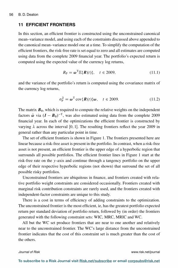
56 B. D. Deaton
11 EFFICIENT FRONTIERS
In this section, an efficient frontier is constructed using the unconstrained canonicalmean–variance model, and using each of the constraints discussed above appended tothe canonical mean–variance model one at a time. To simplify the computation of theefficient frontiers, the risk-free rate is set equal to zero and all estimates are computedusing data from the complete 2009 financial year. The portfolio’s expected return iscomputed using the expected value of the currency log returns,
RP D !TEfR.t/g; t 2 2009; (11.1)
and the variance of the portfolio’s return is computed using the covariance matrix ofthe currency log returns,
�2P D !T covfR.t/g!; t 2 2009: (11.2)
The matrix B0, which is required to compute the relative weights on the independentfactors Q! via .I � B0/�T, was also estimated using data from the complete 2009financial year. In each of the optimizations the efficient frontier is constructed byvarying � across the interval Œ0; 1�. The resulting frontiers reflect the year 2009 ingeneral rather than any particular point in time.
The set of efficient frontiers is shown in Figure 1. The frontiers presented here arelinear because a risk-free asset is present in the portfolio. In contrast, when a risk-freeasset is not present, an efficient frontier is the upper edge of a hyperbolic region thatsurrounds all possible portfolios. The efficient frontier lines in Figure 1 start at therisk-free rate on the y-axis and continue through a tangency portfolio on the upperedge of their respective hyperbolic regions (not shown) that surround the set of allpossible risky portfolios.
Unconstrained frontiers are ubiquitous in finance, and frontiers created with rela-tive portfolio weight constraints are considered occasionally. Frontiers created withmarginal risk contribution constraints are rarely used, and the frontiers created withindependent-factor constraints are unique to this study.
There is a cost in terms of efficiency of adding constraints to the optimization.The unconstrained frontier is the most efficient, ie, has the greatest portfolio expectedreturn per standard deviation of portfolio return, followed by (in order) the frontiersgenerated with the following constraint sets: WIC, MRC, MRIC and WC.
All but the WC set produce frontiers that are near to one another and relativelynear to the unconstrained frontier. The WC’s large distance from the unconstrainedfrontier indicates that the cost of this constraint set is much greater than the cost ofthe others.
Journal of Risk www.risk.net/journal
To subscribe to a Risk Journal visit Risk.net/subscribe or email [email protected]

Decomposition of portfolio risk using an inductive causal search algorithm 57
FIGURE 1 Comparison of efficient frontiers.
0
0.0001
0.0002
0.0003
0.0004
0.0005
0.0006
0 0.01 0.02 0.03 0.04 0.05
Exp
ecte
d re
turn
Standard deviation
UnconstrainedWCWICMRCMRIC
The frontiers are generated using constrained mean–variance optimization with data from 2009. Each frontier in theplot is labeled according to the constraint set used in its creation: the relative portfolio weight constraint (WC) set,the independent-factor relative-weight constraint (WIC) set, the marginal risk contribution constraint (MRC) set andthe independent-factor marginal risk contribution constraint (MRIC) set.
12 PORTFOLIO PERFORMANCE
The performance of each of these portfolios is compared using data that spans 00:00–12:30 on January 4, 2010; the realized returns for each of the six currencies during thistime period are shown in Figure A-3.8 It is assumed that the risk-free rate is zero andthat there are no transaction costs. TheVAR–LiNGAM estimation results from 2009 ofEfn.t/g, covfn.t/g and M1 are used in the time series model that serves as the base forthe portfolio optimizations. The 2009 estimate for B0 is used to compute the relativeweights on the independent factors Q!. For each period’s portfolio optimization, themost recently observed return R.t/ is used to compute the next period’s conditionalexpected value EfR.t C 1/ j M1; R.t/g, as follows:
EfR.t C 1/ j M1; R.t/g D EfM1R.t/ C n.t/ j M1; R.t/gD M1R.t/ C Efn.t/g: (12.1)
The 2009 covariance matrix of the residuals is used for each portfolio optimizationand is assumed to remain constant throughout January 4, 2010.
8 See Appendix A online for the relevant figures referred to in this section.
www.risk.net/journal Journal of Risk
To subscribe to a Risk Journal visit Risk.net/subscribe or email [email protected]

58 B. D. Deaton
FIGURE 2 Portfolio performance comparison on January 4, 2010 from 00:00 to 12:30.
99.8
99.9
100.0
100.1
100.2
100.3
100.4
100.5
100.6
100.7
100.8
100.9
Wea
lth
0 10 20 30 40 50Time
UnconstrainedWCWICMRCMRIC
For every point in time in the plot, the VAR–LiNGAM model is used to generate forecasts, and then constrainedmean–variance optimization is used to rebalance each portfolio. Initial portfolio wealth is 100 CHF. Each portfolio inthe plot is labeled according to the constraint set used in its creation: the relative portfolio weight constraint set (WC),the independent-factor relative-weight constraint set (WIC), the marginal risk contribution constraint set (MRC) andthe independent-factor marginal risk contribution constraint set (MRIC).
Each portfolio is created with � D 0:99 in its corresponding optimization modelfor every time period in the simulation; this high degree of risk aversion was chosenso that the portfolios do not become too volatile. Each portfolio starts with an initialwealth in cash (unallocated to other currencies) of 100 CHF. A comparison of theportfolio performance is shown in Figure 2. The cumulative wealth of each portfolioat any particular point in time in Figure 2 can be explained by comparing the portfolioholdings shown in Figure A-4 with the realized returns shown in Figure A-3. A port-folio experiences a large change in value when it has a large position in a currencythat has a large realized return. For example, in period 30 the unconstrained portfoliohad a substantial loss in value (see Figure 2) because it had a large short (ie, negative)position in the euro (see Figure A-4) and the euro had a large positive return (see Fig-ure A-3). The value of the other portfolios did not change much in period 30 becausenone of them had any substantial positions.
In period 31, the unconstrained portfolio made up the lost ground from the previousperiod by having an even larger short position in the euro and a large short positionin the yen; the yen’s negative return in period 31 was large, while the euro’s was
Journal of Risk www.risk.net/journal
To subscribe to a Risk Journal visit Risk.net/subscribe or email [email protected]

Decomposition of portfolio risk using an inductive causal search algorithm 59
modest. The WC, MRC and MRIC portfolios also experienced large gains in period 31(see Figure 2) by having large short positions in the yen and euro. In period 50, allportfolios lost value because they had long positions in sterling, which had a largenegative return. Overall, on this small data set no one portfolio performed markedlybetter than the others, but the portfolio generated with WIC did seem to lag behind.
Each of the five plots in Figures A-4–A-7 corresponds to a portfolio constructedwith one of the constraints discussed above. All of the plots within a figure displaythe same attribute (eg, percentage marginal risk contributions in Figure A-6) for thepositions contained within a portfolio.
Plots of portfolio currency allocations are shown in Figure A-4; each line in thefigure represents the total value of a particular currency holding in Swiss francs.At some points in time and for all constraints except the weight constraints, theallocation to a specific currency is disproportionately large. Only with the relativeweight constraints are the allocations of all currencies kept within a narrow boundary.
Independent-factor relative portfolio weights over time are displayed in FigureA-5.The WIC and WC sets appear to be the most effective at keeping the independent-factor relative portfolio weights constrained. The other constraint sets allow some ofthe independent-factor relative portfolio weights to become many times larger thanthe others; this concentration of wealth in a small number of independent factors isundesirable because it represents a loss of diversification.
Percentage marginal risk contribution plots are shown in FigureA-6, and independ-ent-factor percentage marginal risk contribution plots are shown in Figure A-7. Noneof the plots in either of these figures indicates that the marginal risk contributionsbecome as divergent as some of the independent-factor relative portfolio weights doin Figure A-5. In this small example, the WC set seems to be almost as effective asthe MRC set at controlling the percentage marginal risk contributions in Figure A-6, whereas the MRIC set is the only constraint set that appears truly effective atcontrolling independent-factor percentage marginal risk contributions in Figure A-7.
13 CONCLUSION
When a portfolio contains a set of correlated assets, a portfolio manager’s life iscomplicated by the fact that risk can only be analyzed relative to an existing portfolio.However the portfolio is constructed, marginal risk analysis is confusing becausechanging the size of one position changes not only its marginal risk contribution butalso the marginal risk contributions from the other positions. To further complicatematters, some positions have negative marginal risk contributions, so increasing sucha position’s size will actually reduce the risk of the portfolio at the margin.
VAR–LiNGAM is presented in this paper as a method of finding a portfolio’s under-lying independent risk factors. Such factors can be used to decompose a portfolio’s
www.risk.net/journal Journal of Risk
To subscribe to a Risk Journal visit Risk.net/subscribe or email [email protected]

60 B. D. Deaton
risk so that the risk contribution from any independent factor is nonnegative. Withthis decomposition, the risk contribution from each independent factor can be inter-preted as having a potentially adverse effect on the portfolio, and portfolios can beconstructed using a risk budget. In the example application, percentage independent-factor risk contributions are constrained to be less than or equal to 25% of the totalportfolio’s risk. This is equivalent to a portfolio manager deciding that no more than25% of the portfolio’s risk should be allocated to any one independent risk factor. Thisdecision takes place before the portfolio is created, and the percentage risk allocationsare not relative to an existing portfolio, as they would be when risk factors are notindependent.
In Section 7, we found the market structure underlying a set of currencies, andfrom this we identified the set of independent factors. Portfolios are constructed on asample data set by constraining the portfolio weights and the percentage marginal riskcontributions of both the original assets and the independent factors during mean–variance optimizations. The properties of the portfolios and efficient frontiers cre-ated using constraints on the independent risk factors compare favorably with thosecreated using constraints on the original assets. Plots of the independent-factor per-centage marginal risk contributions show that the best way to control independent-factor marginal risk contributions is to put constraints on the independent-factor riskmarginal contributions themselves.
DECLARATION OF INTEREST
The author reports no conflicts of interest. The author alone is responsible for thecontent and writing of the paper.
ACKNOWLEDGEMENTS
Thanks to David A. Bessler, James W. Mjelde, David J. Leatham and an anonymousreviewer for helpful comments that improved the quality of the paper.
REFERENCES
Bank for International Settlements (2010). Triennial central bank survey report on globalforeign exchange market activity in 2010. Report, September, Bank for InternationalSettlements. URL: http://bit.ly/SfH8Nl.
Gerard, C., andTutuncu, R. (2007).Optimization Methods in Finance.Cambridge UniversityPress.
Green, R. C. (1992). When will mean–variance efficient portfolios be well diversified?Journal of Finance 47(5), 1785–1809 (http://doi.org/bp6d).
Journal of Risk www.risk.net/journal
To subscribe to a Risk Journal visit Risk.net/subscribe or email [email protected]

Decomposition of portfolio risk using an inductive causal search algorithm 61
Hyvärinen, A. S. (2008). Causal modelling combining instantaneous and lagged effects: anidentifiable model based on non-Gaussianity. In Proceedings of the 25th InternationalConference on Machine Learning, pp. 424–431. International Machine Learning Society,Helsinki, Finland (http://doi.org/bm3fgz).
Hyvärinen, A. S., Karhunen, J., and Oja, E. (2001). Independent Component Analysis.Wiley (http://doi.org/dxw8pj).
Hyvärinen, A. S., Zhang, K., Shimizu, S., and Hoyer, P. O. (2010). Estimation of a struc-tural vector autoregression model using non-Gaussianity. Journal of Machine LearningResearch 11, 1709–1731.
Litterman, R. (1996). Hot Spots and Hedges. Risk Management Series. Goldman, Sachs& Co, New York (http://doi.org/bp6f).
Markowitz, H. (1952). Portfolio selection. Journal of Finance 7(1), 77–91 (http://doi.org/bhzd).
Meucci, A. (2007). Risk contributions from generic user-defined factors. Risk 20(6), 84–88.Popescu, T. D. (2009). Time series forecasting using independent component analysis.
World Academy of Science, Engineering and Technology 25, 667–672.Qian, E. (2006). On the financial interpretation of risk contribution: risk budgets do add up.
Journal of Investment Management 4(4), 1–11.Shaffer, J. (1995). Multiple hypothesis testing. Annual Review of Psychology 46(1), 561–
584 (http://doi.org/dbh5rx).Shimizu, S., Hoyer, P. O., Hyvärinen, A., and Kerminen, A. (2006). A linear non-Gaussian
acyclic model for causal discovery.Journal of Machine Learning Research 7, 2003–2030.Zenios, S. A. (2007). Practical Financial Optimization: Decision Making for Financial
Engineers. Wiley–Blackwell.
www.risk.net/journal Journal of Risk
To subscribe to a Risk Journal visit Risk.net/subscribe or email [email protected]

Journal of Risk 19(1), 63–76DOI: 10.21314/JOR.2016.346
Research Paper
Optimal asset management fordefined-contribution pension fundswith default risk
Shibo Bian,1 James Cicon2 and Yi Zhang3
1School of Finance, Shanghai Lixin University of Accounting and Finance, Shanghai 201620,People’s Republic of China; email: [email protected] School of Business and Professional Studies, University of Central Missouri,Warrensburg, MO 64093, USA; email: [email protected] of Public Economics and Administration, Shanghai University of Finance and Economics,Shanghai 200433, People’s Republic of China; email: [email protected]
(Received September 17, 2015; revised December 4, 2015; accepted January 25, 2016)
ABSTRACT
We explore how a defined-contribution pension fund optimally distributes wealthbetween a defaultable bond, a stock and a bank account, given that a salary is a stochas-tic process. We assume that the investment objective of the defined-contribution pen-sion fund is to maximize the expected constant relative risk aversion utility of terminalwealth. We thus obtain a closed-form solution to the optimal problem using a martin-gale approach. We develop numerical simulations, which we graph as illustrations.Finally, we discuss relevant economic insights obtained from our results.
Keywords: defined-contribution pension plan; optimal investment; defaultable bond; stochasticsalary; martingale approach.
Corresponding author: S. Bian Print ISSN 1465-1211 j Online ISSN 1755-2842Copyright © 2016 Incisive Risk Information (IP) Limited
63
To subscribe to a Risk Journal visit Risk.net/subscribe or email [email protected]

64 S. Bian et al
1 INTRODUCTION
The Latin American debt crisis, the US subprime crisis and the European sovereigndebt crisis serve to remind us that default risk is a major issue facing investors.Furthermore, these crises emphasize the importance of incorporating the default fea-ture into portfolio management models. Consequently, interest in the defaultablemarket-optimal portfolio problem has increased.
Korn and Kraft (2003) studied the optimal portfolio in the context of defaultablebonds and price the defaultable bond using Merton’s (1974) structural approach.They use elasticity and duration as control variables in their optimization problem,expressing the optimal amounts invested in each security as functions of these twovariables. The paper by Kraft and Steffensen (2006) extends their work within a “firstpassage time” framework (Black and Cox 1976).
A parallel branch of literature studies the defaultable asset optimal-portfolio prob-lem within a reduced-form default framework. Walder (2002), Jin and Hou (2002) andHou (2003) study the default risk optimal investment problem under the conditionaldiversification assumption (implying an asymptotic disappearance of the jump-riskpremium). Dynamics with constant jump-risk premium and constant default intensityfor the price process of a defaultable bond are proposed in Bielecki and Jang (2006).Meindl and Primbs (2006) bring transaction costs into the model. They derive the opti-mal investment strategy via the receding-horizon control approach. Bo et al (2010)consider a stochastic portfolio-optimization problem in a defaultable market. Theyassume that the jump-risk premium and the default intensity of the defaultable bondrely on a stochastic factor described by a diffusion process. Biagini and Cretarola(2009, 2012) arrive at the optimal defaultable claim investment strategy through thelocal risk minimizations approach. Bian and Liu (2013) analyze the optimal invest-ment strategy in a defaultable bond, a stock and a bank account using martingalemethods. Capponi and Figueroa-López (2014) use regime switching within a portfoliooptimization framework based on the defaultable bond.
The crises demonstrate that contagion risk plays a fundamental role in financiallydistressed situations. The following representative studies analyze contagion issues.Kraft and Steffensen (2008) analyze the impact of joint default risk on the investor’sportfolio decision, where the investor wishes to invest in defaultable bonds under themultiple default framework of Schönbucher (1998). In a subsequent study, Kraft andSteffensen (2009) consider the impact of contagion on investor demand for default-able bonds. Jiao et al (2013) combine stochastic control and backward stochasticdifferential equation decomposition. This approach permits them to provide gener-alized formulas that explain the terminal wealth and the optimal investment strategywith defaultable bonds. Bo and Capponi (2014) use credit default swaps to analyzehow contagion risk affects the optimal allocation decision.
Journal of Risk www.risk.net/journal
To subscribe to a Risk Journal visit Risk.net/subscribe or email [email protected]

Optimal asset management for defined-contribution pension funds with default risk 65
These representative studies leave a gap in the literature. They focus on the investorwho has a self-financing investment strategy. However, they do not address the fact thatmany investors in defaultable bonds pursue a non-self-financing investment strategy.Such investors include pension funds, insurers and mutual funds.
We aim to fill this gap in the literature. Our paper shows how a defined-contribution(DC) pension fund can invest optimally in defaultable bonds. We show that the DCpension fund’s investment strategy is not self-financing because it experiences con-tinuous contributions. Some studies use a stochastic framework to investigate the DCpension fund’s optimal investment strategy. Such studies include Boulier et al (2001),Haberman and Vigna (2002), Deelstra et al (2004), Menoncin and Scaillet (2006),Zhang et al (2007) and Gao (2008). To the best of our knowledge, we are the firstto study the optimal investment problem of a DC pension fund whose investmentopportunity set includes a default security.
In this paper, we consider a unique investment optimization problem: a DC pensionfund operating in a financial market that provides a defaultable bond, a risky stockasset and a bank account. The fund manager may dynamically share their wealthbetween the three aforementioned assets. They seek to maximize terminal wealthunder a finite horizon of expected utility. We use the martingale approach to obtain aclosed-form solution to this optimization problem.
The paper is organized as follows. In Section 2 we set up the mathematicalframework of our financial market model. In Section 3 we introduce our portfolio-optimization problem. In Section 4 we carry out our numerical analysis. Section 5summarizes our results and concludes our paper. Technical details appear in the onlineappendixes.
2 OUR FINANCIAL MARKET MODEL
We begin building our model by defining our complete probability space, .˝; Ft ; Q/,where Q denotes a risk-neutral (martingale probability) measure which is assumed tobe equivalent to the real-world (statistical) measure P. Next we introduce H.t/, whichis a default stochastic process that jumps at a random time � . Let H.t/ D 1f�6tg, where1f�6tg is the indicator function, which is 0 before the default event and 1 otherwise.
We assume that the pension fund’s investment set is a defaultable bond, a stock anda bank account. In the following we describe the dynamics between these securitiesand wealth.
2.1 The dynamics of financial securities
The promised principal of the defaultable zero-coupon bond is 1. The maturity dateis T1, and the default time is � . Following Duffie and Singleton (1999) we define the
www.risk.net/journal Journal of Risk
To subscribe to a Risk Journal visit Risk.net/subscribe or email [email protected]

66 S. Bian et al
valuation formula for a defaultable zero-coupon bond with price p.t; T1/ as
p.t; T1/ D 1f�>tg � EQ�
exp
��Z T1
t
.r C hQ�/ ds
� ˇ̌ˇ̌ Ft
�; (2.1)
where r is risk-free rate, hQ is default intensity under Q and � is the loss rate. Weassume that all are constant.
Applying Ito’s lemma and H.t/ D 1f�6tg to (2.1), we derive the dynamics of theprice process of the defaultable bond:
dp.t; T1/ D p.t; T1/.r dt � .1 � H.t//� dM Q.t//; (2.2)
where the compensated jump martingale process M Q.t/ is given by
dM Q.t/ D dH.t/ � .1 � H.t//hQ dt:
We assume that the stock price and the bank account are given by the followingdiffusion equation:
dS.t/ D S.t/.r dt C �S dW Q.t//; (2.3)
dB.t/ D rB.t/ dt; (2.4)
where �S is the volatility of the stock and W Q.t/ is a Brownian motion under Q.
2.2 The dynamics of wealth
Contributions payable by both employee and employer are defined under a DC pensionplan. In most cases they correspond to a fixed percentage of the salary. FollowingZhang et al (2007), we assume that the salary of a pension plan member follows thedynamics described below:
dL.t/ D L.t/.� dt C �L1dW Q.t/ C �L2
dM Q.t//; (2.5)
where �L1and �L2
are two volatility scale factors that measure how the risk sourcesof the stock and the defaultable bond affect the salary, and � is the expected growthrate of the salary. We assume that �L1
, �L2and � are constants.
We assume that the initial value of the pension account is x > 0, that the contributionrate is c and that �p.t/, �S.t/, 1��S.t/��p.t/ are the proportions of the pension fundinvested in the defaultable bond, the stock and the bank account respectively. Thus,the corresponding portfolio process X�.t/ is governed by the following equation:
dX�.t/ D X�.t/.�S.t/ dS.t/ C �p.t/ dp.t; T1/ C .1 � �S.t/ � �p.t// dB.t//
C cL.t/ dt: (2.6)
Journal of Risk www.risk.net/journal
To subscribe to a Risk Journal visit Risk.net/subscribe or email [email protected]

Optimal asset management for defined-contribution pension funds with default risk 67
Substituting (2.2)–(2.4) into (2.6), we get
dX�.t/ D X�.t/.r dt C �S� dW Q.t/ � .1 � H.t//�p� dM Q.t// C cL.t/ dt: (2.7)
Note that contributions are assumed to be invested continuously over time. Theexpectation of the plan member’s future contribution enables the pension fund to investthe plan member’s contributions optimally. Therefore, we can state the followingdefinitions.
Definition 2.1 Following Bodie et al (1992) we define the discounted expectedfuture contribution process as
D.t/ D EQ�Z T
t
B.s/
B.t/cL.s/ ds
ˇ̌ˇ̌ Ft
�:
We set D.0/ D d .
Definition 2.2 Following Bodie et al (1992) we define the pension fund wealthprocess V.t/ as
V.t/ D X�.t/ C D.t/: (2.8)
Equation (2.8) should be interpreted as follows: the wealth of the pension fund attime t is equal to the value of the portfolio X�.t/ plus the discounted expected valueof future contributions to the plan.
The process D.t/ is not directly observable. Therefore, it is not certain if thepension fund is likely to base its investment decision upon it. However, an observablealternative is the salary process L.t/. In Lemma 2.3, we show that the processes D.t/
and L.t/ are strongly linked.
Lemma 2.3 The expected future contributions process D.t/ and the salary processL.t/ are related via the equation
D.t/ D 1
�.exp.�.T � t // � 1/cL.t/; (2.9)
where � D � � r .
Proof See Appendix A online. �
Taking derivatives of (2.9) and using (2.5), we have
dD.t/ D D.t/.r dt C �L1dW Q.t/ C �L2
dM Q.t// � cL.t/ dt: (2.10)
Taking derivatives of (2.8) and using (2.7) and (2.10), we have
dV.t/ D V.t/
0BB@r dt C
.X�.t/�S�S C D.t/�L1/ dW Q.t/
C .X�.t/..H.t/ � 1/�p�/ C D.t/�L2/ dM Q.t/
V .t/
1CCA :
www.risk.net/journal Journal of Risk
To subscribe to a Risk Journal visit Risk.net/subscribe or email [email protected]

68 S. Bian et al
Thus, under Q, the discounted wealth process is a martingale:
d
�V.t/
B.t/
�D V.t/
B.t/
0BB@
.X�.t/�S�S C D.t/�L1/ dW Q.t/
C.X�.t/..H.t/ � 1/�p�/ C D.t/�L2/ dM Q.t/
V .t/
1CCA : (2.11)
Therefore, we write
EQ�
V.t/
B.t/
�D V.0/
B.0/D v D x C d:
We change the measure from Q to P. This is necessary because the pension fundoptimizes utility under the real-world probability measure. Following Girsanov’stheorem we use the Radon–Nikodým density martingale Z.t/ D dQ=dP and
EP�
Z.t/V .t/
B.t/
�D EQ
�V.t/
B.t/
�D v; (2.12)
where EP is the expectation under P. Z.t/ should satisfy
EP.Z.t// D 1; Z.t/ D ZW .t/ZH .t/;
where
ZW .t/ D exp
��Z t
0
� dW.s/ � 1
2
Z t
0
�2 ds
�;
ZH .t/ D exp
�Z t
0
ln � dH.s/ �Z t
0
hP.� � 1/.1 � H.s// ds
�:
� is the market price of risk for the stock, � D hP=hQ is the jump-risk premium, hP
is the default intensity under P,
W.t/ D W Q.t/ �Z t
0
� ds
is a Brownian motion under P, and
M.t/ D M Q.t/ � hPZ t
0
.� � 1/.1 � H.s// ds
is a martingale under P.
3 SOLUTION TO THE OPTIMIZATION PROBLEM
The pension fund will maximize the expected utility of terminal wealth. We defineour utility function as U.v/. We define J.v/ as the maximal utility attained by imple-menting the optimal investment strategy ��. We may now define our optimization
Journal of Risk www.risk.net/journal
To subscribe to a Risk Journal visit Risk.net/subscribe or email [email protected]

Optimal asset management for defined-contribution pension funds with default risk 69
problem as
J.v/ D sup�
EP.U.V .T /// such that EP�
Z.t/V .t/
B.t/
�D v: (3.1)
Following Cox and Huang (1989) and Duffie (2010), we use the martingale approachto solve our optimization problem.
3.1 Maximizing general utility
We assume that the utility function U is strictly increasing and strictly concave. Ittherefore follows that the derivative U 0 is strictly decreasing and continuous. It alsofollows that its inverse function, I.Y /, is strictly decreasing and continuous:
I.U 0.V // D V; 0 < V < 1;
U 0.I.Y // D Y; 0 < Y < U 0.0/:
The convex dual of U is the function defined by QU .Y / , supV 2R.U.V / � V Y /. QUreaches its maximum at V D I.Y /, and
U.V / � V Y 6 U.I.Y // � YI.Y /: (3.2)
We interpret Y.v/ as a Lagrange multiplier. We reduce the constrained maximiza-tion problem of (3.1) to the unconstrained problem
EP.U.V .T /// C Y.v/.v � EP.N.T /V .T ///; (3.3)
where N.t/ D Z.t/=B.t/. Applying the result of (3.2), we have
vY.v/ C EP.U.V .T // � Y.v/N.T /V .T //
6 vY.v/ C EP.U.I.Y.v/N.T /// � Y.v/N.T /I.Y.v/N.T /// (3.4)
with equality if and only if
V.T / D I.Y.v/N.T //: (3.5)
Then V.T / is the optimal terminal wealth.Using V.T /, the martingale property of N.t/V .t/ and Ito’s lemma, we get an
alternative expression for d.V .t/=B.t//. Comparing this to the corresponding termsin (2.11), we identify the expressions for the optimal portfolio ��. We summarize ourresults in Proposition 3.1.
www.risk.net/journal Journal of Risk
To subscribe to a Risk Journal visit Risk.net/subscribe or email [email protected]

70 S. Bian et al
Proposition 3.1 Let v be the endowment for the pension. Let V.T / be terminalwealth at time T . There exists an optimal investment strategy ��:
.X��.t/��
S �S C D.t/�L1/
V .t/
V .t/
B.t/D �1.t/ C �.t/�
Z.t/; (3.6)
.X��.t/..H.t/ � 1/��
p �/ C D.t/�L2/
V .t/
V .t/
B.t/D �2.t�/ C .1 � �/�.t�/
�Z.t�/; (3.7)
where
�.t/ D EP.N.T /I.Y.v/N.T // j Ft /; (3.8)
d�.t/ D �1.t/ dW.t/ C �2.t/ dM.t/: (3.9)
Proof See Appendix B online. �
Proposition 3.1 gives a general solution. In Section 3.2, we assume a constantrelative risk aversion (CRRA) utility, which we use to derive the closed-form optimalinvestment strategy.
3.2 Maximizing CRRA utility
Given the pension fund with a CRRA utility function as follows:
U.V / D V �
�; 0 < � < 1:
The inverse function of U 0 is then given by
I.y/ D y1=.��1/: (3.10)
Using (2.12), (3.5) and (3.10), we derive
v D EP.N.T /I.Y.v/N.T /// D Y.v/1=.��1/EP.N.T /�=.��1// (3.11)
and obtain
Y.v/ D�
v
EP.N.T /�=.��1//
�1=.��1/
: (3.12)
Substituting (3.12) into (3.5) and using (3.10), we have the optimal terminal wealth:
V.T / D I.Y.v/N.T //
D v
EP.N.T /�=.��1//N.T /1=.��1/: (3.13)
Journal of Risk www.risk.net/journal
To subscribe to a Risk Journal visit Risk.net/subscribe or email [email protected]

Optimal asset management for defined-contribution pension funds with default risk 71
Substituting (3.13) and N.T / into (3.8) for a CRRA utility yields
�.t/ D v
EP.N.T /�=.��1//EP.N.T /�=.��1/ j Ft /
D vN.t/�=.��1/
EP.N.T /�=.��1//EP��
N.T /
N.t/
��=.��1/ ˇ̌ˇ̌ Ft
�: (3.14)
Applying Ito’s lemma to (3.14) we have
d�.t/
�.t�/D dN.t/�=.��1/
N.t/�=.��1/C d˝.t/
˝.t�/; (3.15)
where
˝.t/ D EP��
N.T /
N.t/
��=.��1/ ˇ̌ˇ̌ Ft
�: (3.16)
Our last step in determining the optimal portfolio is to find (3.15). Lemmas 2.3 and 3.2provide the explicit expressions for
dN.t/�=.��1/
N.t/�=.��1/and
d˝.t/
˝.t�/;
respectively. Given this, we now have d�.t/=�.t�/. Comparing this result with (3.9)yields �.t/. Finally, by substituting the �.t/ into Proposition 3.1, we obtain the explicitoptimal portfolio.
Lemma 3.2 The derivative of N.t/�=.��1/ is given by
dN.t/�=.��1/
N.t/�=.��1/D �
.1 � �/.� dW.t// C .��=.��1/ � 1/ dM.t/ C Œ�� dt: (3.17)
Proof See Appendix C online. �
Lemma 3.3 Given that W.t/ and H.t/ are independent of each other, the derivativeof ˝.t/ is given by
d˝.t/
˝.t�/D�
��=.��1/
��
��=.��1/.1 � exp.hP.T � t ///
C exp
��
� � 1.1 � �/hP C hP.T � t /
���1
� 1
�dM.t/ C Œ�� dt:
(3.18)
Proof See Appendix D online. �
www.risk.net/journal Journal of Risk
To subscribe to a Risk Journal visit Risk.net/subscribe or email [email protected]

72 S. Bian et al
Proposition 3.4 When the defaultable bond is not in default, the optimal strategyof the DC pension fund with the CRRA utility function is given by
��p D 1
��
�� � ��=.��1/
� ��=.��1/
�exp
��
� � 1.1 � �/hP C hP.T � t /
�
C ��=.��1/.1 � exp.hP.T �t///
�C 1
��1 C D.t/
X��.t/
�
� �L2
D.t/
X��.t/
; (3.19)
��S D 1
1 � �
�
�S
�1 C D.t/
X��.t/
�� �L1
�S
D.t/
X��.t/
: (3.20)
Proof Using Proposition 3.1, Lemma 3.2 and Lemma 3.3, we directly obtainProposition 3.4. �
From (3.19), it is clear that the optimal investment strategy for the defaultablebond is a decreasing function of the loss rate � and the volatility of the salary �L2
. Thehigher the loss rate, the smaller the investor recovery. Holding other factors constant,the pension fund allocates a smaller amount of wealth to the defaultable bond. Asthe volatility of the salary increases, the pension fund invests smaller amounts ofwealth in the defaultable bond. We cannot directly observe the influence of the jump-risk premium �, the default intensity hP and the time to maturity on the optimalinvestment strategy for the defaultable bond. Therefore, in the following numericalsimulation we analyze the effect of these factors in the pension fund’s decision.
From (3.20) we know that the optimal investment of the stock is similar to that ofthe defaultable bond. This allows us to proceed to our simulation.
4 SIMULATION
In this section, we develop a numerical simulation that demonstrates the influenceof the jump-risk premium �, the default intensity hP and the time to maturity ofthe optimal investment strategy for the defaultable bond. The initial values of ourparameters are given in Table 1.
Figure 1 provides evidence that there is a positive relationship between optimalinvestment in the defaultable bond and the jump-risk premium �. Holding otherfactors constant, the pension fund purchases more defaultable bonds when the price ofthe jump risk is higher. The optimal investment in the defaultable bond increases witha decreasing rate as the jump-risk premium � increases. When the default intensity
Journal of Risk www.risk.net/journal
To subscribe to a Risk Journal visit Risk.net/subscribe or email [email protected]

Optimal asset management for defined-contribution pension funds with default risk 73
TABLE 1 Parameters for our numerical experiment.
NumericalSymbol Interpretation value
� Jump-risk premium 1–3hP Default intensity 0.01–0.03� Loss rate 0.5
T � t Time to maturity 1–10� Risk aversion coefficient 0.5r Risk-free rate 0.03� Expected growth of salary 0.06
.�L1 ; �L2/0 Volatility of salary (0.05,0.01)0
c Contribution rate 0.15
FIGURE 1 Optimal investment of the defaultable bond versus the jump-risk premium andthe default intensity.
0.010.015
0.020.025
0.033.0
2.52.0
1.01.5
Default intensityJump-riskpremium
Opt
imal
inve
stm
ent o
fde
faul
tabl
e bo
nd
0.6
0.5
0.4
0.3
0.2
0.1
0
hP is low, the marginal increase in the optimal investment strategy for the defaultablebond is huge, and vice versa. We interpret our result with the following in mind: thepension fund responds more to the investment return when the default intensity hP islow, and responds more to the investment risk when the default intensity hP is high.The optimal investment strategy for the defaultable bond is a decreasing function ofthe default intensity hP. Greater default intensity hP leads to a higher probability ofdefault, thus the pension fund allocates smaller amounts of wealth to the defaultablebond.
www.risk.net/journal Journal of Risk
To subscribe to a Risk Journal visit Risk.net/subscribe or email [email protected]

74 S. Bian et al
FIGURE 2 Optimal investment of the defaultable bond versus the jump-risk premium andthe time to maturity.
10987654321 Time to maturity
3.02.5
2.0
1.01.5Jump-risk
premium
Opt
imal
inve
stm
ent o
fde
faul
tabl
e bo
nd
0.5
0.4
0.3
0.2
0.1
0
We provide evidence in Figure 2 that the optimal investment strategy for the default-able bond is an increasing function of time to maturity. The pension fund allocatesmore to defaultable bonds when the investment horizon is longer. When the timeto maturity is long, the marginal increase in the optimal investment strategy for thedefaultable bond becomes huge, and vice versa. We offer the following explanation:the fund manager permits the choice of a more aggressive investment policy andresponds more to the investment return when the time to maturity is long. As thedeadline approaches, the fund manager tends toward a more conservative investmentpolicy.
5 CONCLUSIONS
This paper analyzed the problem of optimal investment in the defaultable bond, givenan investor with a non-self-financing strategy. We showed how to optimally allocatea DC pension fund’s wealth between a defaultable bond, a stock and a bank account(given a salary is a stochastic process). We used a reduced-form approach to model thedefaultable bond, which allowed us to give the dynamics of the defaultable bond. Weassumed that the pension fund’s utility was CRRA and used the martingale approachto obtain a closed-form solution to this optimal problem. Our results provide evi-dence that optimal investment in the defaultable bond is an increasing function ofthe jump-risk premium and the time to maturity. The optimal investment strategy for
Journal of Risk www.risk.net/journal
To subscribe to a Risk Journal visit Risk.net/subscribe or email [email protected]

Optimal asset management for defined-contribution pension funds with default risk 75
the defaultable bond is decreasing in the default intensity, in the loss rate and in thevolatility of salary.
DECLARATION OF INTEREST
This work was supported by the National Natural Science Foundation of China, grant71301105, 71503154. The authors report no conflicts of interest. The authors aloneare responsible for the content and writing of the paper.
REFERENCES
Biagini, F., and Cretarola, A. (2009). Local risk minimization for defaultable markets.Mathematical Finance 19(4), 669–689 (http://doi.org/ftj47q).
Biagini, F., and Cretarola, A. (2012). Local risk-minimization for defaultable claimswith recovery process. Applied Mathematics and Optimization 65(3), 1–22 (http://doi.org/cnwrvm).
Bian, S., and Liu, H. (2013). Optimal investment with a corporate bond. Mathematical andComputer Modelling 58(9), 1615–1624 (http://doi.org/bp4n).
Bielecki, T. R., and Jang, I. (2006). Portfolio optimization with a defaultable security. Asia-Pacific Financial Markets 13(2), 113–127 (http://doi.org/fs9q6r).
Black, F., and Cox, J.C. (1976).Valuing corporate securities: some effects of bond indentureprovisions. Journal of Finance 31(2), 351–367 (http://doi.org/bmnw).
Bo, L., and Capponi, A. (2014). Optimal investment in credit derivatives portfolio undercontagion risk. Mathematical Finance, forthcoming (http://doi.org/bnct).
Bo, L., Wang, Y., and Yang, X. (2010). An optimal portfolio problem in a defaultable market.Advances in Applied Probability 42(3), 689–705 (http://doi.org/bp4p).
Bodie, Z., Merton, R. C., and Samuelson, W. F. (1992). Labor supply flexibility and portfoliochoice in a life cycle model. Journal of Economic Dynamics and Control 16(3), 427–449(http://doi.org/c6v4jn).
Boulier, J. F., Huang, S. J., and Taillard, G. (2001). Optimal management under stochasticinterest rates: the case of a protected defined contribution pension fund. Insurance:Mathematics and Economics 28(2), 173–189 (http://doi.org/dx759w).
Capponi, A., and Figueroa-López, J. E. (2014). Dynamic portfolio optimization with adefaultable security and regime-switching. Mathematical Finance 24(2), 207–249 (http://doi.org/bp4q).
Cox, J. C., and Huang, C. F. (1989). Optimal consumption and portfolio policies whenasset prices follow a diffusion process. Journal of Economic Theory 49(1), 33–83 (http://doi.org/fp7n64).
Deelstra, G., Grasselli, M., and Koehl, P. F. (2004). Optimal design of the guarantee fordefined contribution funds. Journal of Economic Dynamics and Control 28(11), 2239–2260 (http://doi.org/fhn9pq).
Duffie, D. (2010). Dynamic Asset Pricing Theory. Princeton University Press.Duffie, D., and Singleton, K. J. (1999). Modeling term structures of defaultable bonds.
Review of Financial Studies 12(4), 687–720 (http://doi.org/dqf7cr).
www.risk.net/journal Journal of Risk
To subscribe to a Risk Journal visit Risk.net/subscribe or email [email protected]

76 S. Bian et al
Gao, J. (2008). Stochastic optimal control of DC pension funds. Insurance: Mathematicsand Economics 42(3), 1159–1164 (http://doi.org/bt6rgk).
Haberman, S., and Vigna, E. (2002). Optimal investment strategies and risk measures indefined contribution pension schemes. Insurance: Mathematics and Economics 31(1),35–69 (http://doi.org/cvwwvj).
Hou, Y. (2003). Integrating market and credit risk: a dynamic asset allocation perspective.Working Paper, Yale University.
Jiao, Y., Kharroubi, I., and Pham, H. (2013). Optimal investment under multiple defaultsrisk: a BSDE-decomposition approach. Annals of Applied Probability 23(2), 455–491(http://doi.org/bp4r).
Jin, X., and Hou, Y. (2002). Optimal investment with default risk. Working Paper, FAME,University of Lausanne, Switzerland.
Korn, R., and Kraft, H. (2003). Optimal portfolios with defaultable securities a firm valueapproach. International Journal of Theoretical and Applied Finance 6(8), 793–819 (http://doi.org/cqj2xh).
Kraft, H., and Steffensen, M. (2006). Portfolio problems stopping at first hitting time withapplication to default risk. Mathematical Methods of Operations Research 63(1), 123–150 (http://doi.org/bz73g6).
Kraft, H., and Steffensen, M. (2008). How to invest optimally in corporate bonds: a reduced-form approach. Journal of Economic Dynamics and Control 32(2), 348–385 (http://doi.org/ctbhvj).
Kraft, H., and Steffensen, M. (2009).Asset allocation with contagion and explicit bankruptcyprocedures. Journal of Mathematical Economics 45(1), 147–167 (http://doi.org/c8t7fw).
Meindl, P., and Primbs, J. (2006). Corporate bond portfolio optimization with transactioncosts. Working Paper, Stanford University (http://doi.org/fxm8xr).
Menoncin, F., and Scaillet, O. (2006). Optimal asset management for pension funds.Managerial Finance 32(4), 347–374 (http://doi.org/dtghqg).
Merton, R. C. (1974). On the pricing of corporate debt: the risk structure of interest rates.Journal of Finance 29(2), 449–470 (http://doi.org/bhm7).
Schönbucher, P. J. (1998). Term structure modelling of defaultable bonds. Review ofDerivatives Research 2(2), 161–192 (http://doi.org/fk47c7).
Shreve, S. E. (2004). Stochastic Calculus for Finance. Springer.Walder, R. (2002). Dynamic allocation of treasury and corporate bond portfolios. Working
Paper, FAME, University of Lausanne, Switzerland (http://doi.org/b6hdbc).Zhang, A., Korn, R., and Ewald, C. O. (2007). Optimal management and inflation protection
for defined contribution pension plans.Blätter der DGVFM 28(2), 239–258 (http://doi.org/d2w7sn).
Journal of Risk www.risk.net/journal
To subscribe to a Risk Journal visit Risk.net/subscribe or email [email protected]

Journal of Risk 19(1), 77–90DOI: 10.21314/JOR.2016.340
Research Paper
A fuzzy data envelopment analysis model forevaluating the efficiency of sociallyresponsible and conventional mutual funds
I. Baeza-Sampere,1 V. Coll-Serrano,1 B. M’Zali2 andP. Méndez-Rodríguez3
1Department of Applied Economics, University of Valencia, Avenida Dels Tarongers s/n,46022 Valencia, Spain; emails: [email protected], [email protected] of Stratégie, Responsabilité Sociale et Environnementale,Université du Québec à Montréal, Case Postale 8888, Succursale Centre-Ville,Montréal, Canada; email: [email protected] of Quantitative Economics, University of Oviedo, Avenida del Cristo s/n,33006 Oviedo, Spain; email: [email protected]
(Received March 10, 2015; revised September 28, 2015; accepted September 28, 2015)
ABSTRACT
Although several data envelopment analysis (DEA) models have been proposed inthe literature for mutual funds’ performance evaluation, few of them incorporatenonfinancial criteria. In this paper a fuzzy DEA model is used, allowing mutual fundsrelative performance evaluation in a more realistic and flexible way. We examinethe efficiency of forty US large cap equity mutual funds based not only on financialvariables but also on nonfinancial ones. To achieve this aim, we extend Basso andFunari’s mutual funds’ ethical level proposing a more reliable fuzzy measure of thesocial environmental responsibility degree of equity mutual funds. It relies on thecorporate social performance of the companies invested in by the mutual funds andon the quality of the management in terms of the transparency and credibility degreeof the nonfinancial information provided by the mutual funds. We can conclude that
Corresponding author: I. Baeza-Sampere Print ISSN 1465-1211 j Online ISSN 1755-2842Copyright © 2016 Incisive Risk Information (IP) Limited
77
To subscribe to a Risk Journal visit Risk.net/subscribe or email [email protected]

78 I. Baeza-Sampere et al
socially responsible mutual funds show better behavior in terms of efficiency thanconventional funds.
Keywords: socially responsible investment; equity mutual funds; fuzzy data envelopment analysis(DEA); efficiency; quality management; social environmental responsibility.
1 INTRODUCTION
Sustainable and responsible investing (SRI) takes into account not only financialperformance but also the investment’s impact on society. The ways in which SRIimpacts society are numerous. Some examples are the use of active share ownershipand engagement strategies; community investing; or the influence on national andglobal public policies and the development of global standard-setting organizationsas the Carbon Disclosure Project, Ceres, the Council of Institutional Investors or theGlobal Reporting Initiative.
SRI contributes to the improvement of the Environmental Social and Governance(ESG) practices of companies to generate both positive societal impact and long-termcompetitive financial returns (Social Investment Forum 2012). Recently, given thecauses of the 2008 financial crisis, ESG concerns have become more and more rele-vant and SRI is gaining adherents even in investment firms that have not historicallyidentified themselves as SRI firms. As an example, the number of signatories of thePrinciples for Responsible Investment (PRI) is estimated to represent around 20% ofthe estimated total value of global capital markets.
As reported by the Social Investment Forum in its 2010 report (Social InvestmentForum 2010), social investing in the US market enjoyed a growth rate of more than13% from 2007 to 2010 with 250 socially screened mutual fund products in 2010with assets of US$316.1 billion. SRI is therefore a growing and important investmentfield and, consequently, there is an increasing body of academic literature that paysattention to it. Most of the research is focused on the discussion about the financialperformance of SRI, in particular of invested funds or mutual funds (see Rennebooget al 2008, for a review of the academic literature on this topic). Very few studiesevaluate the performance in terms not only of financial but also nonfinancial criteria.Moreover, few of them can be found analyzing their efficiency.
In this paper, we use data envelopment analysis (DEA) to assess the relative effi-ciency of a sample of US equity mutual funds. This paper presents two main con-tributions. First, it extends Pérez-Gladish et al’s social environmental responsibilitymeasurement (Pérez-Gladish et al 2013) proposing a more reliable indicator of theenvironmental responsibility degree of equity mutual funds which relies on the Cor-porate Social Performance of the companies invested in by the mutual funds and onthe transparency and credibility degree of the nonfinancial information provided by
Journal of Risk www.risk.net/journal
To subscribe to a Risk Journal visit Risk.net/subscribe or email [email protected]

The efficiency of socially responsible and conventional mutual funds 79
the mutual funds. The main advantage of the proposed measure is that it includesthe uncertain and/or imprecise nature of some of the considered nonfinancial inputsand outputs. Secondly, by incorporating the fuzzy measure of social environmen-tal responsibility as an input, it extends Basso and Funari’s DEA model (Basso andFunari 2007, 2010, 2012) giving rise to a fuzzy DEA model, which permits mutualfunds relative performance evaluation in a more realistic and flexible way.
The rest of the paper is organized as follows. Section 2 describes the fuzzy DEAmodel used to measure the efficiency scores of US equity mutual funds. Section 3specifies the data and variables used in the application. Section 4 presents the mainresults obtained. Finally, Section 5 shows the main conclusions.
2 METHODOLOGY
Data envelopment analysis (Charnes et al 1994) is a nonparametric technique thatallows evaluation of the relative efficiency of a set of decision-making units (DMUs).Conventional DEA models assume data are precisely measured, but this assumptionis not always acceptable. In this work we assume the uncertainty and/or imprecisioninherent to certain inputs and outputs which we handle through fuzzy numbers.
Let U be a space of points, a fuzzy set in U is QA D f.x; � QA.x//; x 2 U g, where� QA W U ! Œ0; 1� is a function. For each x 2 U , the value � QA.x/ is called thegrade of membership of x in QA (Zadeh 1965). A fuzzy number is a convex andnormalized .supx2U � QA.x/ D 1/ fuzzy set with a piecewise continuous mem-bership function. The most used fuzzy numbers are known as LR-fuzzy numbers(Dubois and Prade 1988). A fuzzy number QM is said to be an LR-fuzzy number,QM D .mL; mR; ˛L; ˛R/L;R, if its membership function has the following form (León
et al 2003; Vercher et al 2007):
� QM D
8ˆ̂̂ˆ̂<ˆ̂̂ˆ̂:
L
�mL � r
˛L
�; r 6 mL;
1; mL 6 r 6 mR;
R
�r � mR
˛R
�; r > mR;
(2.1)
where L and R are reference functions, that is, L; R W Œ0; C1Œ ! Œ0; 1� are strictlydecreasing functions in supp. QM/ D fr W � QM .x/ > 0g and upper semi-continuoussuch that L.0/ D R.0/ D 1. If L and R are linear functions, the fuzzy number is saidto be an LR-fuzzy trapezoidal. The triangular fuzzy number, QM D .m; ˛L; ˛R/L;R,is a special case of the trapezoidal one, where the upper base degenerates to a point(crisp value).
Fuzzy mathematical programming provides a useful tool to deal with this kindof data (León et al 2003). Hatami-Marbini et al (2011) provides a taxonomy and
www.risk.net/journal Journal of Risk
To subscribe to a Risk Journal visit Risk.net/subscribe or email [email protected]
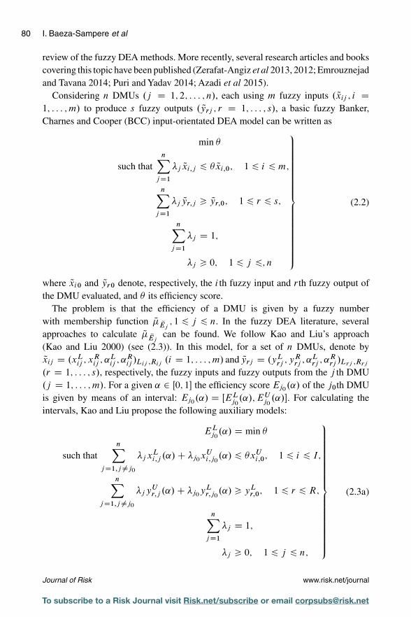
80 I. Baeza-Sampere et al
review of the fuzzy DEA methods. More recently, several research articles and bookscovering this topic have been published (Zerafat-Angiz et al 2013, 2012; Emrouznejadand Tavana 2014; Puri and Yadav 2014; Azadi et al 2015).
Considering n DMUs .j D 1; 2; : : : ; n/, each using m fuzzy inputs . Qxij ; i D1; : : : ; m/ to produce s fuzzy outputs . Qyrj ; r D 1; : : : ; s/, a basic fuzzy Banker,Charnes and Cooper (BCC) input-orientated DEA model can be written as
min �
such thatnX
j D1
�j Qxi;j 6 � Qxi;0; 1 6 i 6 m;
nXj D1
�j Qyr;j > Qyr;0; 1 6 r 6 s;
nXj D1
�j D 1;
�j > 0; 1 6 j 6; n
9>>>>>>>>>>>>>>>>>=>>>>>>>>>>>>>>>>>;
(2.2)
where Qxi0 and Qyr0 denote, respectively, the i th fuzzy input and r th fuzzy output ofthe DMU evaluated, and � its efficiency score.
The problem is that the efficiency of a DMU is given by a fuzzy numberwith membership function Q� QEj
; 1 6 j 6 n. In the fuzzy DEA literature, severalapproaches to calculate Q� QEj
can be found. We follow Kao and Liu’s approach(Kao and Liu 2000) (see (2.3)). In this model, for a set of n DMUs, denote byQxij D .xL
ij ; xRij ; ˛L
ij ; ˛Rij /Lij ;Rij
.i D 1; : : : ; m/ and Qyrj D .yLrj ; yR
rj ; ˛Lrj ; ˛R
rj /Lrj ;Rrj
.r D 1; : : : ; s/, respectively, the fuzzy inputs and fuzzy outputs from the j th DMU
.j D 1; : : : ; m/. For a given ˛ 2 Œ0; 1� the efficiency score Ej0.˛/ of the j0th DMU
is given by means of an interval: Ej0.˛/ D ŒEL
j0.˛/; EU
j0.˛/�. For calculating the
intervals, Kao and Liu propose the following auxiliary models:
ELj0
.˛/ D min �
such thatnX
j D1;j ¤j0
�j xLi;j .˛/ C �j0
xUi;j0
.˛/ 6 �xUi;0; 1 6 i 6 I;
nXj D1;j ¤j0
�j yUr;j .˛/ C �j0
yLr;j0
.˛/ > yLr;0; 1 6 r 6 R;
nXj D1
�j D 1;
�j > 0; 1 6 j 6 n;
9>>>>>>>>>>>>>>>>>=>>>>>>>>>>>>>>>>>;
(2.3a)
Journal of Risk www.risk.net/journal
To subscribe to a Risk Journal visit Risk.net/subscribe or email [email protected]

The efficiency of socially responsible and conventional mutual funds 81
and
EUj0
.˛/ D min �
such thatnX
j D1;j ¤j0
�j xUi;j .˛/ C �j0
xLi;j0
.˛/ 6 �xLi;0; 1 6 i 6 I;
nXj D1;j ¤j0
�j yLr;j .˛/ C �j0
yUr;j0
.˛/ > yUr;0; 1 6 r 6 R;
nXj D1
�j D 1;
�j > 0; 1 6 j 6 n;
9>>>>>>>>>>>>>>>>>=>>>>>>>>>>>>>>>>>;
(2.3b)
where � is the efficiency of the unit being evaluated .j0/ and �j are the weights fromwhich the value � is obtained.
However, the efficiency scores obtained from (2.3) cannot be used to rank units. Ifa unit shows a lower efficiency ratio, this does not guarantee that another unit shouldhave priority over it (Boscá et al 2011). In order to solve this problem and to rankunits, we propose using Chen and Klein’s index (Chen and Klein 1997), which isgiven by
CK. QEj / DPN
lD0.EUj .˛l/ � c/
PNlD0.EU
j .˛l/ � c/ �PN
lD0.ELj .˛l/ � d/
; j D 1; : : : ; n; (2.4)
where
˛l D 1
N; l D 0; : : : ; N;
cl D mini;j
fELi;j .˛l/g;
d D maxi;j
fEUi;j .˛l/g:
3 DATA AND VARIABLES
DEA has been used for assessing the relative performance of mutual funds. Most of theacademic works use a measure of risk (standard deviation of returns, variance, etc) asone of the inputs, and returns (mean return, excess on return, minimum return, skew-ness, etc) as one of the outputs (see, for example, Murthi et al (1997); McMullen andStrong (1998); Morey and Morey (1999); Choi and Murthi (2001); Wilkens and Zhu(2001); Galagedera and Silvapulle (2002); Chang (2004); Briec et al (2004, 2007);Joro and Na (2006); Daraio and Simar (2006); Basso and Funari (2007, 2010, 2012)).
www.risk.net/journal Journal of Risk
To subscribe to a Risk Journal visit Risk.net/subscribe or email [email protected]

82 I. Baeza-Sampere et al
Lozano and Gutiérrez (2008) revise and summarize these inputs and outputs togetherwith technology, formulation, orientation, metric and other interesting remarks of theDEA approaches used for mutual funds’ performance evaluation. But as far as weknow, only Basso and Funari (2007, 2010, 2012) and more recently Pérez-Gladishet al (2013) include nonfinancial variables in their DEA models for mutual fund per-formance evaluation; these authors specifically consider mutual funds’ ethical levelas an output.
A common characteristic of the above-mentioned studies is that they all use conven-tional DEA models, and consequently their evaluations are based on the assumptionof certain and/or precise data. However, these assumptions could not be realistic,mainly due to (i) the difficulty in measuring certain social, environmental and gov-ernance characteristics of the firms and of the social responsibility of mutual fundsor (ii) the uncertainty of financial data. In these cases, fuzzy sets theory is a usefultool to reflect this uncertainty and/or imprecision and to incorporate into the modelinformation based not only on historical data but also on the experts’ knowledge.
In this study, 40 US large cap equity mutual funds were analyzed, 23 of them arelisted members of the Social Investment Forum (SIF) and the remaining 17 wererandomly selected large cap conventional mutual funds. Data comes from the formerKinder, Lydenberg, and Domini Inc (KLD) and Morningstar databases.
We consider two output variables: (1) a fund’s expected return (R), which is theamount one would anticipate receiving on an investment that has various known orexpected rates of return; and (2) a social environmental responsibility (SER) index,which is based on the corporate social performance (CSP) of the firms invested inby the equity mutual fund. This paper uses a well-established database from KLDResearch & Analytics Inc. that takes into account the multidimensional aspects ofCSP (see Pérez-Gladish et al 2012). KLD monitors CSP of US firms according toa set of binary variables, some of which may reflect strengths (S) others concerns(C). In this work, we have transformed concerns into strengths by taking the binarycomplementaries in order to aggregate them (see (3.1)). If a mutual fund does notpresent a certain concern, we will consider this fact as a strength:
CSPk D6X
sD1
Ssk C7X
rD1
Crk; k D 1; : : : ; p; CSPk 2 f0; 1; : : : ; 13g: (3.1)
Once we have obtained a CSP measurement for each of the firms invested in by theconsidered mutual funds, we can obtain an SER value for each mutual fund:
SERj DpX
kD1
˛kj CSPk; j D 1; 2; : : : ; 40; (3.2)
where p is the number of firms invested in by mutual fund j , and ˛kj is the weightingof firm k in mutual fund j .
Journal of Risk www.risk.net/journal
To subscribe to a Risk Journal visit Risk.net/subscribe or email [email protected]

The efficiency of socially responsible and conventional mutual funds 83
As input variables, we propose to use the following.
(1) Standard deviation of the returns rate (SD), which is a traditional risk measurefor the fund investment.
(2) Transaction costs (Murthi et al 1997; Choi and Murthi 2001). This input isrelated to the following variables.
(a) Turnover ratio (TR): this is a measure of the portfolio manager’s tradingactivity, which is computed by taking the lesser of purchases or sales(excluding all securities with maturities of less than 1 year) and dividingby the average monthly net assets.
(b) Gross expense ratio (GER): this represents the total gross expenses (netexpenses with waivers added back in) divided by the funds’ average netassets.
(c) Loads: these loads may be charged at the beginning (front load) whenthe customer invests or they may be deferred till the time the customerwithdraws his/her funds (deferred load).
Table 1 shows some basic descriptive statistics for all of the input and outputvariables defined above.
Thus, values for variables front load and deferred load are considered certain andprecise as the charged amount is generally based on the amount of the investment andthey remain stable along the investment time.
The values of R, SER, SD, TR and GER will be handled through fuzzy numbers inorder to better reflect their uncertainty and to try to incorporate in their constructionthe expert’s knowledge in addition to the available historical data (data series forthe period 1997–2007). Specifically for R, SD and TR, these fuzzy numbers areconstructed as fuzzy triangular LR numbers, where m is the median, and ˛L and ˛R
are random percentages of m.In the case of the social, environmental responsibility index (SER) fuzziness will
be incorporated based on the quality of the nonfinancial information provided by themutual fund.The quality management (QM) dimension tries to reflect the transparencyand credibility of the information provided by the fund related to the nonfinancialscreening and research processes. It includes eleven different criteria (Q), ten of whichwere already considered as criteria in Pérez-Gladish et al (2012) and an additionalcriterion: manager’s SRI competence, which refers to SRI education of the fundmanager. Measurement of this variable is done through binary variables for each ofthe criteria. These variables take value 1 if the quality criterion is satisfied and 0otherwise. The best performance in this dimension implies satisfaction of all criteria.
www.risk.net/journal Journal of Risk
To subscribe to a Risk Journal visit Risk.net/subscribe or email [email protected]

84 I. Baeza-Sampere et al
TAB
LE
1B
asic
desc
riptiv
est
atis
tics
for
allo
fthe
inpu
tand
outp
utva
riabl
es.
Co
nven
tio
nal
mu
tual
fun
ds
SR
Imu
tual
fun
ds
Tota
l.n
D16
/.n
D24
/.n
D40
/‚
…„ƒ
‚…„
ƒ‚
…„ƒ
Var
iab
les
Min
.M
ax.
Mea
nS
DM
in.
Max
.M
ean
SD
Min
.M
ax.
Mea
nS
D
Out
puts
Exp
ecte
dre
turn
(%)
(R)
5.03
15.7
79.
063.
501.
5522
.40
7.92
4.60
1.55
22.4
08.
384.
19
Soc
iale
nviro
nmen
tal
5.62
7.03
6.35
0.45
4.59
7.35
6.49
0.72
4.59
7.35
6.44
0.63
resp
onsi
bilit
y(S
ER
)
Inpu
ts
Sta
ndar
dde
viat
ion
(SD
)4.
2910
.47
5.58
1.52
3.59
5.98
4.79
0.46
3.59
10.4
75.
111.
08
Turn
over
ratio
(%)
(TR
)4
128
64.5
441
.23
8.5
9538
.69
22.4
14
128
49.0
333
.38
Ann
ualr
epor
tgro
ss0.
512.
161.
420.
420.
685.
711.
761.
020.
515.
711.
630.
84ex
pens
era
tio(%
)(G
ER
)
Fron
tloa
ds0
5.75
1.72
2.64
05.
251.
222.
160
5.75
1.42
2.34
Def
erre
dlo
ads
05
0.5
1.26
05
11.
870
50.
81.
65
Journal of Risk www.risk.net/journal
To subscribe to a Risk Journal visit Risk.net/subscribe or email [email protected]

The efficiency of socially responsible and conventional mutual funds 85
FIGURE 1 Social environmental responsibility (SER) fuzzy number.
0
1
α
0
1
α
0
1
α
QM = 11 SER QM = 7 SER QM = 1 SER
Source: authors’ own compilation.
Funds not verifying any of the criteria are considered as the worst in terms of QM.(Pérez-Gladish et al 2012, 2013):
QMj D11X
tD1
Qtj ; j D 1; : : : ; 40; QMj 2 f0; 1; : : : ; 11g: (3.3)
The SER fuzzy number was computed taking into account the QM, that is to say,transparency and credibility of the information provided by the fund related to thescreening and research process. In this sense, the higher the QM the higher ourconfidence on the SER’s value.
For a fixed crisp SER, Figure 1 shows how to obtain the SER’s triangular LR-fuzzynumber for different values of QM. The values ˛L and ˛R represent a percentage ofSER which decreases quadratically according to the value of QM. As we can observe,for mutual funds satisfying all the QM criteria (ie, QM D 11), there is no uncertaintyrelated to the transparency and credibility of the information provided by the fund,so the value of the variable measuring the SER of the fund is represented by a crispor precise number. On the other hand, the lower the number of QM criteria satisfiedby the fund, the greater the uncertainty about the SER level of the fund, this leadingto a bigger support of the SER fuzzy numbers.
4 EMPIRICAL RESULTS AND DISCUSSION
Since fuzzy numbers R, SER, SD, TR and GER are randomly obtained by considering˛L, ˛R an arbitrary percentage between 0% and 5% of their values, we generated500 different scenarios in order to obtain more consistent results and to avoid resultsinfluenced by a particular situation. For each of these scenarios the models specifiedin (2.3) were estimated. Then, the average of the funds’ scores was calculated. Table 3in Appendix A, available online, shows the achieved results.
www.risk.net/journal Journal of Risk
To subscribe to a Risk Journal visit Risk.net/subscribe or email [email protected]

86 I. Baeza-Sampere et al
TABLE 2 Chen–Klein Index results and ranking.
Fund Chen–Klein Rank Fund Chen–Klein Rank
S5 1 1 S15 0.8744 8S9 1 1 S1 0.8729 9S16 1 1 S14 0.8713 10S17 1 1 S7 0.8586 11S18 1 1 S8 0.8586 12S19 1 1 C31 0.8509 13S22 1 1 C45 0.8447 14S24 1 1 S3 0.8248 15S25 1 1 S2 0.8192 16C27 1 1 C34 0.7883 17C38 1 1 C44 0.7846 18C41 1 1 C35 0.7533 19C46 1 1 C37 0.6996 20C28 1 1 C29 0.6895 21C33 0.9931 2 C36 0.5922 22S11 0.9496 3 C30 0.5708 23S10 0.9453 4 S26 0.5395 24S12 0.9448 5 C40 0.3029 25S13 0.9296 6 S20 0.0210 26S6 0.9233 7 S21 0.0014 27
S denotes socially responsible mutual fund. C denotes conventional fund.
A total of 14 funds, representing 35% of the funds analyzed, are efficient in allsimulated scenarios and for any ˛-cut. Of these, 9 are socially responsible funds (S5,S9, S16, S17, S18, S19, S22, S24 and S25) and 5 conventional funds (C27, C28, C38,C41 and C46).
The funds that are inefficient have, on average, high scores. A total of 12 SRI fundsand 6 conventional funds attain efficiency ratios above 90%. Possibly, these resultshappen due to the fact that virtually all funds invest in similar portfolios, leaving littleroom for “innovation” and thus limiting the possibility that certain funds significantlystand out above the rest. However, it is interesting to observe the poor ratios attainedby socially responsible funds S20 and S21, and to a lesser extent by the conventionalmutual fund C40.
In order to rank the analyzed mutual funds we have calculated the Chen–Kleinindex (see (2.4)). Obtained results are shown in Table 2.
Obviously, for the 14 funds that are efficient in all scenarios, the Chen–Klein indexis set to 1 and these funds are ranked in the first position. As shown in Table 2,conventional fund C33 ranks second in the ranking. The next 10 funds in the ranking
Journal of Risk www.risk.net/journal
To subscribe to a Risk Journal visit Risk.net/subscribe or email [email protected]

The efficiency of socially responsible and conventional mutual funds 87
are socially responsible funds, with values for the Chen–Klein index moving between0.9496 for mutual fund S11 (position 3) and 0.8586 for mutual fund S8 (position 12).Therefore, of the 25 funds best placed in terms of efficiency, 19 are socially responsiblefunds, which represents 76% of the considered funds.
From the results obtained, it is worth mentioning, undoubtedly, the bad behaviorof funds S20 and S21, which are relegated to the last two positions in the ranking.Indeed, mutual fund S20 presents efficiency scores that are between 0.669 and 0.6693at the lower limit and between 0.6693 and 0.6696 at the upper limit. For mutual fundS21 efficiency ratios are between 0.6624 and 0.6627 at the lower limit and between0.6627 and 0.663 at the upper limit.
Numerous mutual funds rankings exist and are publicly available in order toassist individual investors in their investment decisions, based only on financialvariables. The proposed model in this paper allows ranking mutual funds based ontheir relative efficiency, which is defined in terms of both financial and nonfinancialcriteria.
The efficiency scores obtained can be incorporated by the investor in his/herdecision-making model for portfolio selection together with the classical budget andshort sales constraints and with any other financial or nonfinancial constraints.
5 CONCLUSIONS
In this study, Kao and Liu’s auxiliary fuzzy DEA models (Kao and Liu 2000) have beenapplied in order to evaluate 40 US equity mutual funds. With the aim of classifyingthe mutual funds’ efficiency scores Chein and Klein index has been used.
The main contributions of this work are two: firstly, uncertainty and/or imprecisionof the data is incorporated in the model, leading to a more realistic evaluation of therelative performance of the mutual funds. Secondly, a nonfinancial output is consid-ered, the SER, which is related to the transparency and credibility of the nonfinancialinformation provided by the fund (QM), and it allows us to evaluate the performanceof mutual funds in terms of their efficiency.
The results obtained show that 14 mutual funds (35%) are efficient. From theseefficient funds, 9 (64.3%) are socially responsible listed funds. Moreover, from the25 best positioned funds, 19 are nonconventional mutual funds. Thus, all in all, wecan conclude that, if the expert knowledge is considered together with the historicalinformation, socially responsible mutual funds show a better performance in terms ofefficiency than conventional mutual funds. The investor can incorporate the informa-tion provided by the fuzzy DEA analysis in the decision-making about the portfolioselection.
www.risk.net/journal Journal of Risk
To subscribe to a Risk Journal visit Risk.net/subscribe or email [email protected]

88 I. Baeza-Sampere et al
DECLARATION OF INTEREST
This research has been financially supported by the Spanish Ministry of Science andInnovation (project ECO2011-28927). The authors report no conflicts of interest. Theauthors alone are responsible for the content and writing of the paper.
ACKNOWLEDGEMENTS
We would like to thank Blanca Pérez-Gladish for her comments on previous versionsof this paper.
REFERENCES
Azadi, M., Jafarian, M., Saen, R. F., and Mirhedayatian, S. M. (2015). A new fuzzy DEAmodel for evaluation of efficiency and effectiveness of suppliers in sustainable supplychain management context. Computers & Operations Research 54, 274–285 (http://doi.org/bp4v).
Basso, A., and Funari, S. (2007). DEA models for ethical and non ethical mutual funds.Mathematical Methods in Economics and Finance 2(1), 21–40.
Basso, A., and Funari, S. (2010). Relative performance of SRI equity funds: an analysis ofEuropean funds using data envelopment analysis. Working Paper 201, Department ofApplied Mathematics, University of Venice.
Basso, A., and Funari, S. (2012). Constant and variable returns to scale DEA models forsocially responsible investment funds. Working Paper 20, Department of Economics,University of Venice.
Boscá, J. E., Liern, V., Sala, R., and Martínez, A. (2011). Ranking decision making unitsby means of soft computing dea models. International Journal of Uncertainty, Fuzzinessand Knowledge-Based Systems 19, 115–134 (http://doi.org/br5hrq).
Briec, W., Kerstens, K., and Lesourd, J. B. (2004). Single-period Markowitz portfolio selec-tion, performance gauging and duality: a variation on the Luenberger shortage function.Journal of Optimization Theory and Applications 1201, 1–27 (http://doi.org/c2tb5h).
Briec, W., Kerstens, K., and Jokung, O. (2007). Mean–variance–skewness portfolio perfor-mance appraisals:a general shortage function and dual approach.Management Science531, 135–149 (http://doi.org/fsjrr5).
Chang, K. P. (2004). Evaluating mutual fund performance: an application of minimum con-vex input requirement set approach. Computers and Operations Research 31, 929–940(http://doi.org/bgd2qk).
Charnes, A., Cooper, W. W., Lewin, A. Y., and Seiford, L. M. (1994). Data Envel-opment Analysis: Theory, Methodology and Applications. Kluwer Academic (http://doi.org/cts88m).
Chen, C.B., and Klein, C.M. (1997).An efficient approach to solving fuzzy MADM problems.Fuzzy Sets and Systems 88, 51–67 (http://doi.org/fb8d2s).
Choi, Y. K., and Murthi, B. P. S. (2001). Relative performance evaluation of mutual funds:a non-parametric approach. Journal of Business Finance and Accounting 28, 853–876(http://doi.org/djczzf).
Journal of Risk www.risk.net/journal
To subscribe to a Risk Journal visit Risk.net/subscribe or email [email protected]

The efficiency of socially responsible and conventional mutual funds 89
Daraio, C., and Simar, L. (2006). A robust nonparametric approach to evaluate and explainthe performance of mutual funds.European Journal of Operational Research 175, 516–542 (http://doi.org/fbr52s).
Dubois, D., and Prade, H. (1988). Fuzzy numbers: an overview. In Analysis of FuzzyInformation, Bezdek, J. (ed), Volume 2, pp. 3–39. CRC Press, Boca Raton, FL.
Emrouznejad, A., and Tavana, M. (eds) (2014). Performance Measurement with FuzzyData Envelopment Analysis, Studies in Fuzziness and Soft Computing. Springer.
Galagedera, U. A., and Silvapulle, P. (2002). Australian mutual fund performance appraisalusing data envelopment analysis. Managerial Finance 28, 60–73 (http://doi.org/cxg86z).
Hatami-Marbini, A., Emrouznejad, A., Tavana, M. (2011). A taxonomy and review of thefuzzy data envelopment analysis literature: two decades in the making.European Journalof Operational Research 214(3), 457–472 (http://doi.org/cwq7qp).
Joro, T., and Na, P. (2006). Portfolio performance evaluation in a mean–variance–skewness framework. European Journal of Operational Research 175, 446–461 (http://doi.org/c4dpr3).
Kao, C., and Liu, S. T. (2000). Fuzzy efficiency measures in data envelopment analysis.Fuzzy Sets and Systems 113(3): 427–437 (http://doi.org/c7kws3).
León, T., Liern, V., Ruíz, J. L., and Sirvent, I. (2003). A fuzzy mathematical programmingapproach to the assessment efficiency with DEA models. Fuzzy Sets and Systems 139,407–419 (http://doi.org/ft6jj2).
Lozano, S., and Gutiérrez, E. (2008). TSD-consistent performance assessment of mutualfunds. Journal of the Operational Research Society 59, 1352–1362 (http://doi.org/dtrn8h).
Mansini, R., Ogryczak, W., and Ruszczynski, A. (2003). LP solvable models for portfoliooptimization: a classification and computational comparison. IMA Journal of Manage-ment and Mathematics 14, 187–220 (http://doi.org/fbqgfk).
McMullen, P.R., and Strong, R.A. (1998).Selection of mutual funds using data envelopmentanalysis. Journal of Business and Economic Studies 4, 1–12.
Morey, M. R., and Morey, R. C. (1999). Mutual fund performance appraisals: a multi-horizon perspective with endogenous benchmarking. Omega 27, 241–258 (http://doi.org/d4n485).
Murthi, B.P.S., Choi,Y.K., and Desai, P. (1997).Efficiency of mutual funds and portfolio per-formance measurement: a non-parametric approach. European Journal of OperationalResearch 98, 408–418 (http://doi.org/fc46mp).
Pérez-Gladish, B., Méndez, P., and M’Zali, B. (2012). Ranking socially responsible mutualfunds. International Journal of Energy Optimization and Engineering 1, 59–84 (http://doi.org/bp4w).
Pérez-Gladish, B., Méndez, P., and M’Zali, B. (2013). Mutual funds efficiency measure-ment under financial and social responsibility criteria. Journal of Multi-Criteria DecisionAnalysis 20(3–4), 109–125 (http://doi.org/bp4x).
Puri, J., and Yadav, S. P. (2014). A fuzzy DEA model with undesirable fuzzy outputs andits application to the banking sector in India. Expert Systems and Applications 41(14),6419–6432 (http://doi.org/bp4z).
Renneboog, L., Horst, J. T., and Zhang, C. (2008). Socially responsible investments: insti-tutional aspects, performance and investor behavior. Journal of Banking & Finance 329,1723–1742 (http://doi.org/bt2mg7).
www.risk.net/journal Journal of Risk
To subscribe to a Risk Journal visit Risk.net/subscribe or email [email protected]

90 I. Baeza-Sampere et al
Restzlaff-Roberts, D.L., and Morey, R.C. (1993).A goal-programming method of stochasticallocative data envelopment analysis. European Journal of Operational Research 71(3),379–397 (http://doi.org/d8xknj).
Social Investment Forum (2010). Report on socially responsible investing trends in theUnited States. Social Investment Forum, Washington, DC.
Social Investment Forum (2012). Making a difference: the impact of sustainable andresponsible investment. Social Investment Forum, Washington, DC.
Stolp, C. (1990). Strengths and weaknesses of data envelopment analysis: an urban andregional perspective. Computers, Environment and Urban Systems 14(2), 103–116(http://doi.org/btjqck).
Vercher, E., Bermúdez, J. D., and Segura, J. V. (2007). Fuzzy portfolio optimization underdownside risk measures. Fuzzy Sets and Systems 158, 769–782 (http://doi.org/c7n6cb).
Wilkens, K., and Zhu, J. (2001). Portfolio evaluation and benchmark selection: a math-ematical programming approach. Journal of Alternative Investments 4, 9–20 (http://doi.org/bsvhz9).
Zadeh, L. A. (1965). Fuzzy sets. Information and Control 8, 338–353 (http://doi.org/fcf6rc).Zerafat-Angiz, M.L., and Mustafa, A. (2013).Fuzzy interpretation of efficiency in data envel-
opment analysis and its application in a non-discretionary model. Knowledge-BasedSystems 49, 145–151 (http://doi.org/bp42).
Zerafat-Angiz, M. L., Emrouznejad, A., and Mustafa, A. (2012). Fuzzy data envelopmentanalysis: a discrete approach. Expert Systems with Applications 39, 2263–2269 (http://doi.org/drhkgs).
Journal of Risk www.risk.net/journal
To subscribe to a Risk Journal visit Risk.net/subscribe or email [email protected]