voltage regulation method for voltage drop compensation...

0885-8977 (c) 2016 IEEE. Personal use is permitted, but republication/redistribution requires IEEE permission. See http://www.ieee.org/publications_standards/publications/rights/index.html for more information.

This article has been accepted for publication in a future issue of this journal, but has not been fully edited. Content may change prior to final publication. Citation information: DOI 10.1109/TPWRD.2017.2694836, IEEETransactions on Power Delivery

1

Abstract--Owing to the development of highly efficient electric

power converters, the number of studies on the construction of

low-voltage DC (LVDC) systems is gradually increasing. To use

LVDC distribution systems, voltage regulation methods to

compensate for the voltage drop and to limit the voltage

unbalance are essential. In a bipolar LVDC distribution system, a

voltage drop and voltage unbalance could occur because of the

load current and the variation in the amount of power supplied to

the poles. However, not enough research has been conducted on

voltage regulation methods for LVDC distribution systems. To

reduce the voltage drop and the voltage unbalance, this paper

proposes a voltage regulation method based on the neutral to line

drop compensation (NLDC) method, which employs a modified

LDC to calculate the sending-end reference voltage. In the NLDC

method, the neutral current and neutral line impedance are taken

into consideration to compensate for the neutral line potential

fluctuation and voltage drop on the pole. The next sending-end

voltage is determined by checking the voltage unbalance factor,

and it is adjusted to maintain it within the allowable voltage

unbalance factor. A voltage regulation algorithm and a bipolar

LVDC system model are implemented using ElectroMagnetic

Transients Program.

Index Terms--Line drop compensation, low voltage DC

distribution system, NLDC, voltage drop, voltage unbalance.

I. INTRODUCTION

O reduce the energy losses, various studies on improving

the power efficiency have been performed worldwide. In

this paper, the low-voltage DC (LVDC) distribution system is

investigated as a solution to the power efficiency problem,

because of its many advantages. With a dc distribution system,

power conversion within the appliance can be avoided and

losses reduced. Moreover, the LVDC system is well suited for

connection of various renewable energy systems such as

photovoltaic and fuel cells producing DC power by reducing

the number of conversions: DC/DC/AC to DC/DC conversion.

In addition, the efficiency of the microturbine and variable

speed wind turbine that produce the AC power can be

improved in an LVDC system by reducing the number of

conversions: AC/DC/AC to AC/DC conversion [1]–[6].

The authors are with the College of Information and Communication

Engineering, Sungkyunkwan University, Suwon City, 16419, South Korea (e-

mail: [email protected]; [email protected]; [email protected];

[email protected]; [email protected]; [email protected] ).

An LVDC distribution system can be constructed as a

unipolar or a bipolar system. A unipolar LVDC distribution

system has only one voltage level with two wires, making it

impossible to meet the voltage requirements of all electronic

devices. On the other hand, a bipolar LVDC distribution

system transfers DC power through three wires. In a bipolar

system, various voltage levels can be implemented, which can

decrease the potential to ground in the conductors. However, if

the capacity of the loads connected to each pole is different,

voltage unbalance can occur, which can adversely affect the

receiving voltage [7], [8].

In order to solve the voltage unbalance problem in a bipolar

LVDC distribution system, a dual-buck and half-bridge

balancer that keeps the positive pole voltage equal to the

negative pole voltage has been proposed and studied [7]–[10].

In addition, a buck-boost type balancer and a dual-buck half-

bridge type balancer have been proposed to be employed as

the requirements for power quality increase [11], [12].

However, they operate in the perspectives of electric power

converters rather than the balancer output voltage by voltage

drop on the distribution line. The voltage drop on the

distribution line may reduce the receiving voltage, which

makes the voltage regulation method for the LVDC

distribution system necessary to supply an appropriate voltage

level. In AC systems, the voltage drop is compensated in the

distribution line by stepping up the sending voltage using the

line drop compensation (LDC) method [13]–[20]. However,

this method cannot calculate the proper voltage level taking

into account the neutral potential fluctuation in a bipolar

LVDC distribution system because it considers only the line

current. This means that the LDC method cannot take into

consideration the fluctuation of the neutral potential in a

bipolar LVDC distribution system.

Voltage unbalance and the voltage drop are closely related

to power quality in distribution systems. Therefore, this paper

proposes a technique for voltage regulation in a bipolar LVDC

distribution system that employs neutral to line drop

compensation (NLDC) and restrains the voltage unbalance

factor (VUF). This NLDC method uses the neutral current and

the neutral line equivalent impedance for solving the neutral

line potential fluctuation. The VUF restraint is achieved by

using the objective function of the sending-end reference

voltage (SERV) and the sending-end voltage (SEV). The

Voltage Regulation Method for Voltage Drop

Compensation and Unbalance Reduction in

Bipolar Low-Voltage DC Distribution System Tack-Hyun Jung, Gi-Hyeon Gwon, and Chul-Hwan Kim, Senior Member, IEEE, Joon Han, Yun-Sik

Oh, and Chul-Ho Noh

T



2

voltage regulation method with the NLDC method and VUF

restraint is implemented by using EMTP and MATLAB.

Various cases are simulated in order to verify its validity.

II. VOLTAGE DROP AND UNBALANCE IN BIPOLAR LVDC

DISTRIBUTION SYSTEM

A. Load Voltage in Bipolar LVDC Distribution System

In a bipolar LVDC distribution system, the line current

output from the positive pole I+ of the rectifier returns to the

negative pole I− of the rectifier as shown in Fig. 1. Assuming

the balanced load condition, the magnitudes of the currents

flowing on the poles are equal, i.e., |I+| = |I−|. Because the

current of each pole flows in the opposite direction, the

magnitude of the current flowing in the neutral line becomes

zero. However, assuming the unbalanced load state, the

currents flowing on the poles are unequal, i.e., |I+| ≠ |I−|, so that

the current flowing on the neutral conductor becomes |I+ − I−|

by Kirchhoff’s current law [7], [8].

Fig. 1. Circuit diagram of bipolar LVDC system.

The receiving-end voltage of the positive pole VR+ and the

negative pole VR− are also affected by the current flowing

through the neutral line as well as the current flowing in each

pole, as shown in (1) and (2). This means that in order to

calculate the load voltage exactly in the unbalanced load

condition, the current flowing on the neutral line needs to be

measured. The second terms of (1) and (2) represent the

magnitude of the neutral line potential fluctuation, which is

determined by the current flowing in the neutral line and the

neutral line impedance rN [21].

NLRS rIIrIVV )( (1)

NLRS rIIrIVV )( , (2)

where rL is the pole line impedance and VS+ and VS

− are the

sending voltages of the positive and the negative pole,

respectively.

B. Allowable Voltage Range

The voltage magnitude of the distribution network is the

most important index for evaluating its soundness. Utilities

measure the maximum and minimum customer voltages of

each feeder in order to ensure the both values are within the

allowable voltage range specified in the standard. Table I

shows the allowable voltage range specified in the Korea

Electric Power Corporation (KEPCO) standard, which restricts

the customer voltage variation within 5%–10% of each

nominal voltage. However, this standard is based on AC

voltage. According to Low Voltage Directive (LVD)

2006/95/EC, the range of the low voltage level is existent and

that is between 75-1500Vdc. However, there are no standards

for the allowable voltage variation range of DC yet. It,

therefore, is difficult to verify whether the proposed method in

this paper can satisfy the allowable voltage range for DC.

Instead, this paper has verified that the proposed method can

follow a reference voltage using the performance index, which

is described in more detail for its calculation in Section V. B.

TABLE I

ALLOWABLE VOLTAGE RANGE ACCORDING TO KEPCO STANDARD

Nominal voltage [V] Allowable range [V]

220 207 to 233 (±13)

380 342 to 418 (±38)

6,600 6,000 to 6,900 (-600 to +300)

22,900 20,800 to 23,800 (-2100 to +900)

C. Definition of Voltage Unbalance

Under the unbalanced condition, the bipolar LVDC

distribution system experiences the occurrence of high neutral

current. As a result, this neutral current leads to the power loss

on the neutral conductor and this loss makes it difficult for the

operator to manage the LVDC distribution system. In addition,

under a severe unbalanced situation as the worst case, the

neutral conductor can be burned down due to the excessive

neutral current and the similar case has been occurred in

KEPCO distribution system actually. Thus, the severe voltage

unbalance can cause the potentially unstable condition. To

restrain the VUF, especially in AC distribution system, ANSI

C84.1-1995, developed by National Electrical Manufacturers

Association (NEMA), recommends that electrical supply

systems be designed and operated to limit the maximum

voltage unbalance within 3% [22].

In this paper, we present the VUF in the LVDC system as

the voltage magnitude of the positive and negative poles,

following the NEMA standard as shown in (3) because the

voltage of the LVDC system has no frequency and phase [23]:

1002/)(

%),(),(

),(),(

dcdc

dcdc

VV

VVVUF (3)

III. VOLTAGE REGULATION USING LINE DROP COMPENSATION

The LDC method aims to keep the voltage constant at a

certain point of the distribution line. Voltage control using the

LDC method is performed by calculating the LDC parameters

(center voltage VCE and equivalent impedance Zeq) to

compensate for the voltage drop by the line current IL. Fig. 2

illustrates the concept of determining the SERV using the LDC

method [24]. The concept of the LDC method can be

expressed by (4), which consists of the LDC parameter and the

line current [13]:



3

)(tIZVV LeqCESER (4)

Fig. 2. Voltage regulation using LDC method.

The LDC parameter can be determined by measuring the

line current and the maximum and minimum customer voltage

(Vn,max and Vn, min, respectively) as well as by calculating the

SERV. Equation (5) gives the objective function, which

represents how much the maximum and minimum customers’

feeder voltages are close to the nominal voltage Vnom. The

SERV of a specific distribution system is determined by

employing the minimum condition of (5), where the number of

feeders is N [13],[15]:

N

n

nnomnnom VVVVJMin1

2

min,

2

max, )()( (5)

The equivalent impedance and the load center voltage can

be obtained with the minimum condition (∂J2/∂VCE+∂J2/Zeq =

0) of (6) using the analytic least mean square method as shown

in (7) and (8) [13], [15]–[16]:

N

n

LeqCESER tIZVVJMin1

2

2 )(( (6)

T

t

L

T

t

L

SER

T

t

L

T

t

SER

T

t

L

eq

tITtI

tVtITtVtI

Z

1

2

2

1

111

)()(

)()()()( (7)

T

t

L

T

t

Leq

T

t

SER

T

t

L

CE

tI

tIZtVtI

V

1

1

2

11

)(

)()()( (8)

Here, because the ground potential fluctuation due to the

unbalance current of the neutral line in the bipolar system is

not considered, the LDC parameters depend only on the line

current. The ground potential fluctuation of the neutral line

affects the load voltage and should be considered for accurate

calculation of the voltage drop compensation in a bipolar

system.

IV. THE PROPOSED VOLTAGE CONTROL METHOD

A. Impact of Neutral Line Potential Fluctuation on Load

Voltage

The voltage on the receiving-end VR is determined by the

sending-end voltage VSE, the line voltage drop ΔVL, and the

ground potential fluctuation of the neutral line ΔVn as shown in

Fig. 3 and (9). The conventional LDC method compensates for

only the pole voltage drop presented in the second term of (9).

The proposed NLDC method considers both the pole voltage

drop and the ground potential fluctuation of the neutral line

presented in the third term of (9). The sign of the third term is

determined by the direction of the unbalance current due to the

load unbalance. Depending on the direction of the neutral line

current, the neutral line potential fluctuation intensifies the

voltage drop of one pole applied to the larger load.

nLSER VVVV (9)

Fig. 3. Load voltage by voltage drop and ground potential of neutral line.

B. Calculation of NLDC Parameter

To reflect the effect of the neutral line potential fluctuation,

the NLDC method includes the equivalent impedance of the

neutral line Zeqn. Accordingly, the SERV in the NLDC method

can be represented by (10), which includes the magnitude of

the neutral line current In. The first and second terms on the

left-hand side in (10) are the NLDC parameters, which

compensate for the voltage drop of the pole line, and the third

term is the NLDC parameter, which compensates for the

neutral line potential fluctuation. Fig. 4 shows the concept of

the NLDC method considering the neutral current and the

neutral line equivalent impedance. The SERV of the specific

distribution line can be determined by the equation of the

plane in three-dimensional coordinates:

)()( tIZtIZVV neqnLeqCESER (10)

Fig. 4. Concept of NLDC method considering neutral current.

C. Algebraic Least Mean Square Method by Using SVD

In the analytic least mean square method of (7) and (8), each

parameter can be determined by solving two simultaneous

equations. In the NLDC method, however, three simultaneous



4

equations need to be solved to determine each parameter.

Solving the three simultaneous partial differential equations is

such a complicated procedure that we calculate each parameter

using the algebraic least mean square method. It can be

implemented by gathering the SERV, line current (IL), and

neutral line current (In) of the distribution system. The

gathered data are then organized in matrix form as shown in

(11). By solving the inverse matrix of A (A−1), we can

determine the NLDC parameter.

BxA

NV

V

V

V

V

Z

Z

NINI

II

II

II

SER

SER

SER

SER

CE

eqn

eq

nL

nL

nL

nL

)(

)3(

)2(

)1(

1)()(

1)3()3(

1)2()2(

1)1()1(

(11)

In (11), the inverse matrix of A is nonexistent because it is

not a square matrix. In this paper, thus, we use the pseudo-

inverse, which is used to compute a “best-fit” solution to a

system of linear equations, to solve (11). A simple and

accurate way to compute the pseudo-inverse is by using

Singular Value Decomposition (SVD). If the size of the matrix

is m-by-n, the SVD of A is given as follows:

TVUA , (12)

where U is the orthonormal eigenvector of AAT, V is the

orthonormal eigenvector of ATA, and Σ is the following m-by-n

matrix [25]:

0000

000

000

0001

N

, (13)

where σ is the singular value of matrix A, and we obtain the

pseudo-inverse as (14) by taking the reciprocal of each

nonzero element on the diagonal, leaving the zeros in place,

and then transposing the matrix. In numerical computation,

only elements larger than some small tolerance are taken to be

nonzero, and the others are replaced by zeros [26].

T

N

UVA

0000

0/100

000

000/1 1

1

(14)

By multiplying the inverse matrix of A on both sides of (11),

we can calculate each parameter of matrix x, which consists of

the equivalent impedance, the neutral line equivalent

impedance, and the load center voltage. The procedure to

calculate the NLDC parameters is presented as the flowchart in

Fig. 5.

Calculate the SERV

Transform linear equation to matrix form

Conduct the SVD on matrix A

Calculate the pseudo-inverse matrix

Derive the NLDC paramerter

Zeq, Zeqn,VCE

START

Data acquisition(current of line and neutral,

maximum and minimum

customer voltage)

END

Fig. 5. Flowchart for calculation of NLDC parameter.

D. VUF Control

If the load difference between the positive pole and the

negative pole is large, the SERV calculated from the NLDC

parameter may exceed the allowable range of the VUF [19]–

[20]. In this paper, to suppress the VUF along the entire

distribution line, the SERV is adjusted to restrict the VUF to

the allowable range. Equations (15) and (16) give the ranges of

the allowable VUF (ε) for each standard. The VUF tolerance

band of the SERV is presented as a schematic diagram in Fig.

6. When the SERVs of the positive and negative poles are

located between the two graphs, the allowable VUF is satisfied.

Fig. 6. VUF tolerance band of SERV.

NSERPSERNSERPSER VVifVV ,,,, ,200

200

(15)

http://en.wikipedia.org/wiki/Singular_value_decomposition



5

NSERPSERNSERPSER VVifVV ,,,, ,200

200

(16)

To cooperate with the voltage drop compensation, if the

measured VUF exceeds the allowable range, we adjust the

SERV so that it stays within the boundary condition of the

allowable VUF. Equation (17) is the objective function that

expresses the difference between the SERV and the SEV. The

SEV under the condition that the VUF exceeds the allowable

range is determined by employing the minimum condition

(∂Q/∂VSER,P or ∂Q/∂VSER,N) of the objective function.

2

,,

2

,, )()( NSENSERPSEPSER VVVVQ (17)

By employing the minimum condition to the objective

function, in this case using ∂Q/∂VSER,P, we calculate the SEV

of the positive pole from (18), where the K shown in (20) is

the constant that is determined by the allowable VUF and the

SERVs of the positive and negative poles. By dividing (18) by

K, the SEV of the negative pole is calculated with (19).

12

,,

2

,

K

KVVKV NSERPSER

PSE (18)

12

,,

,

K

VKVV NSERPSER

NSE (19)

NSERPSER

NSERPSER

VVif

VVif

K

,,

,,

,200

200

,200

200

(20)

Fig. 7 shows the flowchart of the proposed voltage

regulation using the NLDC method and the VUF restraints.

The SERV determined with the NLDC parameter is calculated

from the measured line current and the neutral line current.

The VUF of the positive and negative poles is then measured.

If the VUF lies within the allowable range, the SERV

calculated with the NLDC parameter becomes the SEV

without any adjustment. If not, the SERV is adjusted in

accordance with (18) and (19) in order to satisfy the standard

of the VUF.

START

SERV calculation

VSER,P=IP·Zeq.P+In·Zeqn.P+VCE.P

VSER,N=IN·Zeq.N+In·Zeqn.N+VCE.N

ε200

ε200K

ε200

ε200K

no

1K

VKVV

1K

KVVKV

2

NSER,PSER,

NSE,

2

NSER,PSER,

2

PSE,

END

? ε 200VV

VV

NSER,PSER,

NSER,PSER,

yes no

yes

NSER,PSER, VV

NSER,NSE,

PSER,PSE,

V)(V

V)(V

t

t

Input the voltage control element

(Zeq, Zeqn, VCE)

Neutral and pole line current acquisition

(IP, In, IN)

Fig. 7. Flowchart of the proposed voltage regulation method.

V. SIMULATION AND RESULTS

A. Modeling of the LVDC Distribution System

To verify the proposed voltage regulation method, a radial

bipolar LVDC system is modeled as shown in Fig. 8. An

AC/DC converter is used to interconnect the AC grid and DC

grid, and a boost balancer is used to supply the regulated

voltage to both the positive and negative poles. The receiving

ends designated N-2 to N-5 are modeled as a step-down

DC/DC converter and resistive load. ACSR (160 mm2) for two

poles and ACSR (95 mm2) for the neutral line are modeled,

and the length between each receiving end is 200m. More

detailed parameter is tabulated in Table II.

TABLE II

DATA OF SIMULATION SYSTEM

Model Explanation

AC/DC

converter 3-phase SPWM full-bridge converter

DC/DC

converter Typical buck converter with fixed duty ratio

Pole

conductor

ACSR 160mm2 (Rin: 0.39cm, Rout: 0.91cm,

Resistance(DC): 0.182Ω/km)

Neutral

conductor

ACSR 95mm2 (Rin: 0.225cm, Rout: 0.675cm,

Resistance(DC): 0.301Ω/km)

Length between loads 200m

Load Resistive load, each load is 30kW (4.8133Ω)

Line voltage ±750Vdc

Customer voltage 380Vdc



6

In this paper, a simple buck DC/DC converter with fixed

duty ratio is adopted. It is proper in terms of economics

because the distribution system has many loads and requires a

lot of DC/DC converters with high capacity. In EMTP

simulation, the converter is modeled using the Transient

Analysis of Control System (TACS) element and MODELS

function, which is the user defined model based on Fortran

interface. This EMTP does not provide the model of power

electronic converter and semiconductor switch. Therefore, the

semiconductor switch is modeled using an antiparallel diode

element and TACS-controlled TYPE 13 switch, which has

on/off action according to control signal. This signal is

generated through MODELS.

The control type of buck DC/DC converter used in this

paper is the fixed duty ratio, which is one of the several control

method such as PWM. Since this paper focuses on the line

voltage and neutral current in the LVDC distribution system,

the simple and typical method to control the buck converter is

used. The control signal of this buck converter is generated by

the pulse train depending on the duty ratio in MODELS.

N-2

LP1

~=

=

=

==

LP5

N-3

LP2

=

=

LP6

=

=

~=: AC/DC converter

(380Vac / ±750Vdc)

: Buck DC/DC

converter

(750Vdc / 380Vdc)

: load

feeder

N-4

LP3

=

=

LP7

N-5

LP4

=

=

LP8

==

==

==

Boost

Balancer

N-1

AC

grid

Fig. 8. Simulation system.

In order to simulate the load magnitude variation with time,

we use the daily load curve expressed as a percentage as

shown in Fig. 9, which is taken from the actual load data

during the day for the summer season in Korea. Table III

shows the simulation conditions. We simulate the unbalanced

load condition by fixing the load capacity of the negative pole

as 120 kW and by changing that of the positive pole.

TABLE III

SIMULATION CONDITIONS

Case Ratio of load capacity

(Positive : Negative)

Load Unbalance

Factor[%]

Allowable

VUF[%]

1 1.0 : 1.0 0

3

2 1.1 : 1.0 9.52

3 1.2 : 1.0 18.18

4 1.3 : 1.0 26.09

5 1.4 : 1.0 33.33

6 1.5 : 1.0 40

With respect to the simulation model, we collect the SERV,

line current, and neutral current data and represent them as

dots to calculate the LDC and NLDC parameters as shown in

Figs. 9 and 10. Fig. 10 shows the measured data and graphical

expression of the LDC parameter. Fig. 11 shows the measured

data and the graphical depiction of the NLDC parameter.

Table IV shows the voltage regulation parameter for each

method. TABLE IV

VOLTAGE REGULATION PARAMETER FOR EACH METHOD

Method LDC or NLDC parameter

Fixed

voltage

dcPSER VV 750,

dcNSER VV 750,

LDC 294.73223.0, PPSER IV

294.73223.0, NNSER IV

NLDC 108.748129.0092.0, nPPSER IIV

108.748129.0092.0, nNNSER IIV

Fig. 9. Daily load curve for simulation.

Fig. 10. Measured data and LDC parameter of simulation model.

Fig. 11. Measured data and NLDC parameter of simulation model.

B. Simulation Results

1) Voltage drop compensation results

Fig. 12 shows the maximum and minimum customer-end

voltages of Case 4 when the fixed voltage method is applied.

As shown in Fig. 12, the voltage drop of the positive pole is

relatively larger than that of the negative pole. These results



7

are due not only to the difference between the voltage drop of

each pole, but also to the potential fluctuation of the neutral

line. As mentioned before, the potential fluctuation of the

neutral line intensifies the voltage drop of the pole supplying a

large load, while suppressing the voltage drop of the pole

supplying a light load. As shown in Fig. 13, the larger the

voltage unbalance, the larger the potential fluctuation of the

neutral.

(a) positive pole (b) negative pole

Fig. 12. Simulation results of Case 4 (fixed voltage method).

Fig. 13. Ground potential of neutral line for simulation cases.

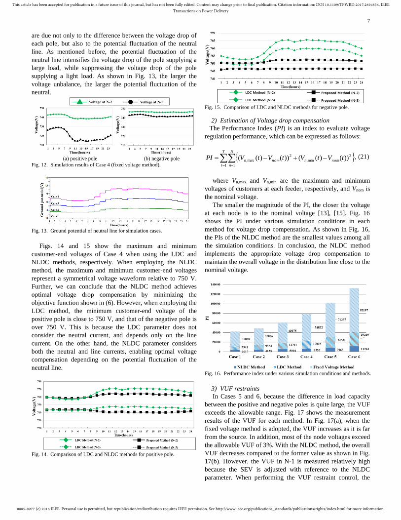
Figs. 14 and 15 show the maximum and minimum

customer-end voltages of Case 4 when using the LDC and

NLDC methods, respectively. When employing the NLDC

method, the maximum and minimum customer-end voltages

represent a symmetrical voltage waveform relative to 750 V.

Further, we can conclude that the NLDC method achieves

optimal voltage drop compensation by minimizing the

objective function shown in (6). However, when employing the

LDC method, the minimum customer-end voltage of the

positive pole is close to 750 V, and that of the negative pole is

over 750 V. This is because the LDC parameter does not

consider the neutral current, and depends only on the line

current. On the other hand, the NLDC parameter considers

both the neutral and line currents, enabling optimal voltage

compensation depending on the potential fluctuation of the

neutral line.

Fig. 14. Comparison of LDC and NLDC methods for positive pole.

Fig. 15. Comparison of LDC and NLDC methods for negative pole.

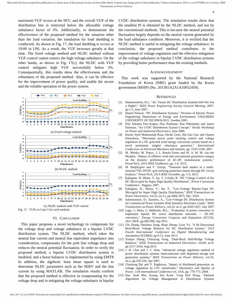
2) Estimation of Voltage drop compensation

The Performance Index (PI) is an index to evaluate voltage

regulation performance, which can be expressed as follows:

T

t

N

n

nomnnomn tVtVtVtVPI1 1

2

min,

2

max, ))()(())()(( , (21)

where Vn,max and Vn,min are the maximum and minimum

voltages of customers at each feeder, respectively, and Vnom is

the nominal voltage.

The smaller the magnitude of the PI, the closer the voltage

at each node is to the nominal voltage [13], [15]. Fig. 16

shows the PI under various simulation conditions in each

method for voltage drop compensation. As shown in Fig. 16,

the PIs of the NLDC method are the smallest values among all

the simulation conditions. In conclusion, the NLDC method

implements the appropriate voltage drop compensation to

maintain the overall voltage in the distribution line close to the

nominal voltage.

Fig. 16. Performance index under various simulation conditions and methods.

3) VUF restraints

In Cases 5 and 6, because the difference in load capacity

between the positive and negative poles is quite large, the VUF

exceeds the allowable range. Fig. 17 shows the measurement

results of the VUF for each method. In Fig. 17(a), when the

fixed voltage method is adopted, the VUF increases as it is far

from the source. In addition, most of the node voltages exceed

the allowable VUF of 3%. With the NLDC method, the overall

VUF decreases compared to the former value as shown in Fig.

17(b). However, the VUF in N-1 is measured relatively high

because the SEV is adjusted with reference to the NLDC

parameter. When performing the VUF restraint control, the



8

maximum VUF occurs at the SEV, and the overall VUF of the

distribution line is restricted below the allowable voltage

unbalance factor of 3%. Additionally, to demonstrate the

effectiveness of the proposed method for the situation other

than the load variation, the simulation for load shedding is

conducted. As shown in Fig. 17, the load shedding is occurs at

19:00 in LP6. As a result, the VUF increases greatly at that

time. The fixed voltage method and NLDC method without

VUF control cannot restrict the high voltage unbalance. On the

other hands, as shown in Fig. 17(c), the NLDC with VUF

control mitigates high VUF successfully below 3%.

Consequentially, this results show the effectiveness and the

robustness of the proposed method. Also, it can be effective

for the improvement of power quality, and enable the secure

and the reliable operation of the power system.

(a) Fixed voltage method

(b) NLDC method

(c) NLDC method with VUF control

Fig. 17. VUFs in Case 5 for each method.

VI. CONCLUSION

This paper proposes a novel technology to compensate for

the voltage drop and voltage unbalance in a bipolar LVDC

distribution system. The NLDC method, which takes the

neutral line current and neutral line equivalent impedance into

consideration, compensates for the pole line voltage drop and

reduces the neutral potential fluctuation. In order to verify the

proposed method, a bipolar LVDC distribution system is

modeled, and a boost balancer is implemented by using EMTP.

In addition, the algebraic least mean square is used to

determine NLDC parameters such as the SERV and the line

current by using MATLAB. The simulation results confirm

that the proposed method is effective in compensating for the

voltage drop and in mitigating the voltage unbalance in bipolar

LVDC distribution systems. The simulation results show that

the smallest PI is obtained by the NLDC method, and not by

the conventional methods. This is because the neutral potential

fluctuation largely depends on the neutral current generated by

the load unbalance condition. Moreover, it is verified that the

NLDC method is useful in mitigating the voltage unbalance. In

conclusion, the proposed method contributes to the

improvement of voltage regulation and the effective mitigation

of the voltage unbalance in bipolar LVDC distribution systems

by providing better performance than the existing methods.

ACKNOWLEDGEMENT

This work was supported by the National Research

Foundation of Korea (NRF) grant funded by the Korea

government (MSIP) (No. 2015R1A2A1A10052459).

REFERENCES

[1] Hammerstrom, D.J., "AC Versus DC Distribution Systems-Did We Get

it Right?," IEEE Power Engineering Society General Meeting, 2007,

pp.1-5, June 2007.

[2] Daniel Nilsson, “DC Distribution Systems,” Division of Electric Power

Engineering Department of Energy and Environment CHALMERS

UNIVERSITY OF TECHNOLOGY, Sweden 2005.

[3] Pasi Salonen, Tero Kaipia, Pasi Nuutinen, Pasi Peltoniemi and Jarmo

Partanen, “An LVDC Distribution System Concept,” Nordic Workshop

on Power and Industrial Electronics, June 2009.

[4] Kazmi Syed Muhammad Raza, Hiroki Goto, Hai-Jiao Guo and Osamu

Ichinokura, “Maximum power point tracking control and voltage

regulation of a DC grid-tied wind energy conversion system based on a

novel permanent magnet reluctance generator,” International

Conference on Electrical Machines and Systems, pp. 1533-1538, 2007.

[5] M. Ndreko, M. Popov, J. L. Rueda-Torres and M. A. M. M. van der

Meijden, “Impact of offshore wind and conventional generation outages

on the dynamic performance of AC-DC transmission systems,”

PowerTech, 2015 IEEE Eindhoven, pp. 1-6, 2015.

[6] M. Hadjikypris and V. Terzija, “Transient fault studies in a multi-

terminal VSC-HVDC grid utilizing protection means through DC circuit

breakers,” PowerTech, 2013 IEEE Grenoble, pp. 1-6, 2013.

[7] Kakigano. H, Miura. Y, Ise, T, Uchida, R, “DC Voltage Control of the

DC Micro-grid for Super High Quality Distribution”, Power Conversion

Conference - Nagoya, 2007.

[8] Kakigano, H.; Miura, Y.; Ise, T., "Low-Voltage Bipolar-Type DC

Microgrid for Super High Quality Distribution," IEEE Transactions on

Power Electronics, vol.25, no.12, pp.3066-3075, Dec. 2010.

[9] Salomonsson, D.; Sannino, A., "Low-Voltage DC Distribution System

for Commercial Power Systems With Sensitive Electronic Loads," IEEE

Transactions on Power Delivery, vol.22, no.3, pp.1620-1627, July 2007.

[10] Lago, J.; Moia, J.; Heldwein, M.L., "Evaluation of power converters to

implement bipolar DC active distribution networks — DC-DC

converters," Energy Conversion Congress and Exposition (ECCE),

2011 IEEE, pp.985-990, Sep 2011.

[11] Chi Zhang; Daozhuo Jiang; Huan Zheng; Lixin Ye, "A Bi-Directional

Buck/Boost Voltage Balancer for DC Distribution System," 2013

Fourth International Conference on Digital Manufacturing and

Automation (ICDMA), pp.9-13, June 2013.

[12] Xianjin Zhang; Chunying Gong, "Dual-Buck Half-Bridge Voltage

Balancer," IEEE Transactions on Industrial Electronics, vol.60, no.8,

pp.3157-3164, Aug 2013.

[13] J. H. Choi and J. C. Kim, "Advanced voltage regulation method of

power distribution systems interconnected with dispersed storage and

generation systems," IEEE Transactions on Power Delivery, vol.16,

no.2, pp.329-334, Apr 2001.

[14] Chensong Dai and Y. Baghzouz, "Impact of distributed generation on

voltage regulation by LTC transformer," Harmonics and Quality of

Power, 11th International Conference on, USA, pp. 770-773, 2004.

[15] Dae. Seok Rho, Kyung Soo Kook, Yong Peel Wang, “Optimal

Algorithms for Voltage Management in Distribution Systems



9

Interconnected with New Dispersed Sources”, Journal of Electrical

Engineering & Technology, Vol. 6, No. 2, pp. 192-201, 2011.

[16] Yun-Seok Ko, “The On-Line Voltage Management and Control Solution

of Distribution Systems Based on the Pattern Recognition Method”,

Journal of Electrical Engineering & Technology, Vol. 4, No. 3, 330 pp.

330~336, 2009.

[17] P. P. Barker and R. W. De Mello, "Determining the impact of

distributed generation on power systems. I. Radial distribution systems,"

Power Engineering Society Summer Meeting, Seattle, vol. 3, pp.1645-

1656, 2000.

[18] J. M. Triplett and S. A. Kufel, "Implementing CVR through voltage

regulator LDC settings," Rural Electric Power Conference (REPC),

2012 IEEE, Milwaukee, pp.B2-1-B2-5, 2012.

[19] C. A. Smith, M. A. Redfern and S. Potts, "Improvement in the

performance of on-load tap changer transformers operating in series,"

Power Engineering Society General Meeting, vol.3, 2003.

[20] Tsai-hsiang Chen, Min-sian Wang, Nien-che Yang, "Impact of

Distributed Generation on Voltage Regulation by ULTC Transformer

using Various Existing Methods," Proceedings of the 7th WSEAS

International Conference on Power Systems, Beijing, China, September

15-17, 2007.

[21] Boeke, Ulrich, and Matthias Wendt. "Comparison of low voltage AC

and DC power grids." Philips Research, AE Eindhoven, Netherlands.

[22] American National Standard for Electric Power Systems Equipment—

Voltage Ratings (60 Hertz), ANSI C84.1-1995.

[23] Von Jouanne, A.; Banerjee, B., "Assessment of voltage unbalance,"

IEEE Transactions on Power Delivery , vol.16, no.4, pp.782,790, Oct

2001.

[24] A. L. M. Mufaris, J. Baba, S. Yoshizawa and Y. Hayashi,

"Determination of dynamic line drop compensation parameters of

voltage regulators for voltage rise mitigation," 2015 International

Conference on Clean Electrical Power (ICCEP), Taormina, pp.319-325,

2015.

[25] Klema, V.; Laub, A.J., "The singular value decomposition: Its

computation and some applications," IEEE Transactions on Automatic

Control, vol.25, no.2, pp.164-176, Apr 1980.

[26] Golub, Gene H.; Charles F. Van Loan (1996). Matrix computations (3rd

ed.). Baltimore: Johns Hopkins. pp. 257–258.

Tack-Hyun Jung was received the B.S. and M.S.

degrees from College of Information and

Communication Engineering, Sungkyunkwan

University, Suwon, Republic of Korea, in 2013 and

2015, respectively.

His research interests include power system

protection and stability in DC distribution systems.

Gi-Hyeon Gwon received his B.S. and M.S. degrees

from College of Information and Communication

Engineering from Sungkyunkwan University,

Suwon, Republic of Korea, in 2012 and 2014,

respectively, where he is currently pursuing the Ph.D.

degree in electrical engineering.


transients, protection, and stability in DC

distribution system.

Chul-Hwan Kim (M’90-SM’04) received the B.S.,

M.S. and Ph.D. degrees in Electrical Engineering

from Sungkyunkwan University, Suwon, Republic

of Korea, in 1982, 1984, and 1990, respectively.

In 1990, he joined Jeju National University, Jeju,

Republic of Korea, as a full-time Lecturer. He has

been a visiting academic at the University of Bath,

UK, in 1996, 1998, and 1999. Since March 1992, he

has been a professor in the College of Information

and Communication, Sungkyunkwan University,

Republic of Korea.

His research interests include power system protection, artificial

intelligence application for protection and control, modeling/protection of

underground cables, and EMTP software.

Joon Han received his B.S. degree from School of E

lectrical Engineering, Soonchunhyang University, A

san, Republic of Korea, in 2011 and his M.S. degree

from College of Information and Communication E

ngineering, Sungkyunkwan University, Suwon, Rep

ublic of Korea, in 2013, where he is currently pursui

ng Ph.D. degree in electrical engineering.

His research interests include power system trans

ients, protection, and stability in DC system.

Yun-Sik Oh received his B.S. and M.S. degrees

from College of Information and Communication

Engineering, Sungkyunkwan University, Suwon,

Republic of Korea, in 2011 and 2013, respectively,

where he is currently pursuing the Ph.D. degree in

electrical engineering.


transients, protection, and stability.

Chul-Ho Noh received the B.S. degree from College

of Information and Communication Engineering,

Sungkyunkwan University, Suwon, Republic of Korea,

in 2013, where he is currently pursuing combined

Ph.D. degree in electrical engineering.


transients, power quality, and protection schemes and

coordination, especially in DC distribution systems.

http://en.wikipedia.org/wiki/Gene_H._Golub

http://en.wikipedia.org/wiki/Charles_F._Van_Loan

voltage regulation method for voltage drop compensation...

Documents