VOLCANIC ASH CLOUD HEIGHTS USING THE

MODIS CO2-SLICING ALGORITHM

by

Michael S. Richards

A thesis submitted in partial fulfillment of the requirements for

the degree of

Master of Science

(Atmospheric and Oceanic Sciences)

at the

UNIVERSITY OF WISCONSIN - MADISON

2006

i

Abstract

To make accurate volcanic ash cloud dispersion forecasts, certain parameters, including the

altitude of the volcanic cloud, must be known. There are several methods used for estimating

the height of an ash cloud, including correlation with ground-based video, correlation with

wind data, cloud-shadow geometry, and the space-borne “11µm brightness temperature”

technique. We introduce the Moderate Resolution Imaging Spectroradiometer (MODIS)

“CO2-slicing” technique as a method for retrieving volcanic cloud heights from space. This

paper compares the heights retrieved from the CO2-slicing method with heights estimated by

the aforementioned methodologies, as well as height products from the Multiangle Imaging

SpectroRadiometer (MISR). This paper also suggests a cloud emissivity correction to the

CO2-slicing algorithm in consideration of volcanic ash clouds

CO2-slicing heights are found to agree well with operational methodologies for the majority

of cases investigated in this study. For two stratospheric volcanic ash clouds, CO2-slicing

heights were within the height estimate window determined by operational methods. Six

tropopause cases were investigated and the CO2-slicing height retrievals were found to be

within ±25hPa for two of the cases, with a third yielding a CO2-slicing estimate within

±50hPa. Height retrieval comparisons with MISR’s stereo height retrieval algorithm,

including a pixel-to-pixel comparison of the two methods, show the MODIS CO2-slicing

height product to generally underestimate the height of the volcanic ash clouds; however,

variability in the two data sets is similar. The CO2-slicing methodology is determined to

ii

under-perform when retrieving heights for 1) lower-altitude volcanic ash clouds and 2)

optically thin volcanic ash clouds.

A cloud emissivity correction is also applied to the CO2-slicing algorithm. A cloud

emissivity ratio of 1.07 is used for the MODIS band36/band35 channel combination, and a

ratio of 0.93 is substituted for the remaining four channel pairs. These emissivity

adjustments raise the CO2-slicing heights for fourteen of fifteen volcanic ash clouds, with an

average increase of 755.4 meters.

iii

Acknowledgements

The work that is presented in this paper would not have been possible without the help of the

following individuals. I would like to thank my advisors Dr. Steve Ackerman and Wayne

Feltz for giving me the opportunity to take on this project and for directing me through to its

completion. I would also like to thank all at the Space and Science Engineering Center, the

Cooperative Institute for Meteorological Satellite Studies, and the Department of

Atmospheric and Oceanic Studies at the University of Wisconsin-Madison for providing a

friendly and professional atmosphere that has truly been a pleasure to work in. Specifically, I

would like to recognize Dr. Bryan Baum for his patience and willingness to lend insight into

the details of the CO2-slicing algorithm, as well as Liam Gumley, Kathy Strabala, and

Richard Frey for their help in answering my MODIS and computer coding questions. I also

wish to recognize Mike Pavolonis for his willingness to share his knowledge and research on

volcanic ash.

This thesis is a compilation of cases whose completion required the assistance of numerous

individuals across the globe. This author wishes to recognize Andrew Tupper of the Darwin

Volcanic Ash Advisory Centre, Australia for his unbelievable help in analyzing many of the

volcanic eruptions presented in this work, as well as for sharing his sources, data, and

personal knowledge that truly made this study possible. In addition, this author wishes to

recognize Catherine Moroney of the Jet Propulsion Laboratory in Pasadena, California, for

her continuing patience in answering MISR questions, as well as her willingness to take time

out of her own work to crunch new data for me. I would like to thank Sergey Senyukov of

iv

the Research Laboratory of Seismic and Volcanic Activity, Kamchatkan Experimental-

Methodical Seismological Department, Russia for sharing his data and new, unpublished

technique on the estimation of volcanic ash plumes. I would also like to thank Yasuhiro

Kamada of the Tokyo Volcanic Ash Advisory Centre for his assistance with the Sheveluch

eruption of 21 May 2001. Also presented in this study is an as-yet unpublished pixel-to-pixel

MODIS/MISR comparison algorithm that was written at this point in time to facilitate work

presented in this paper. For this, I would sincerely like to acknowledge the code’s author

Mike Garay of the Jet Propulsion Laboratory.

The foundation of this work is a CO2-slicing algorithm version written by Greg McGarragh

at the SSEC/CIMSS, University of Wisconsin-Madison (now with the NASA Langley

Research Center). To Greg, I wish to extend a sincere ‘thank you’ for his extreme patience

and assistance in helping me understand the code, as well his very prompt replies to

questions and his willingness to take time to adjust his work to accommodate mine.

This research was supported by the NASA LaRC Subcontract #4400071484.

v

Table of Contents

I. Introduction ……………………………………………………………………………. 1

II. Direct impacts of volcanic ash on aircraft ……………………………………………... 5

III. Current methods for estimating volcanic ash cloud height …………………………… 8

IV. The Moderate Resolution Imaging Spectrometer (MODIS) ………………………... 17

V. CO2-slicing algorithm at 1000-meter resolution ……………………………………... 21

VI. The Multi-angle Imaging SpectroRadiometer (MISR) ……………………………... 32

VII. MISR height retrieval ……………………………………………………………… 36

VIII. CO2-slicing heights compared with MISR heights ……………………………….. 40

IX. CO2-slicing heights compared

with operational height estimation methods …………………………………….. 53

X. CO2-slicing heights compared with

heights estimated by video and photographic techniques ………………………... 65

XI. Changes to the CO2-slicing methodology in consideration of volcanic ash ………... 69

XII. Conclusions and Future Work ……………………………………………………... 77

XIII. References ………………………………………………………………………… 82

XIV. Appendices …………………………………….………………………………….. 88

1

I. Introduction Volcanic ash suspended in the atmosphere poses significant threats to aviation. The

problems posed by airborne volcanic ash are not limited to the relatively minor financial and

aircraft coordination inconveniences sustained by airlines when diversion around ash clouds

is necessary. Rather, threats include loss of life that can occur with flight into airborne

volcanic ash clouds, as well as the significant financial liabilities incurred with severely

damaged aircraft, both of which may be direct results of airborne encounters with ash.

Due to the hazards posed by airborne volcanic ash, detection, monitoring, and the forecasting

of the position of volcanic eruption clouds is necessary to ensure aircraft and passenger

safety. Figure 1 shows how significant the volcanic ash cloud threat is to aviation, as the

major North Pacific air routes come close to over 100 potentially active volcanoes. Between

1985 and 2000, over 100 jet aircraft were damaged due to unexpected encounters with

volcanic ash, and the financial cost to commercial aircraft due to volcanic ash is estimated to

have surpassed $250(US) (Simpson et al., 2000a). Avoidance of ash might be a relatively

trivial issue when in close proximity to an erupting volcano in clear skies. However,

volcanic ash is a significant hazard even at far distances from the eruption (Casadevall,

1994). While an ash plume emitting from a volcano might be easily recognizable in clear

skies due to its location and visual attributes, the ash cloud might become difficult to

recognize as it drifts from its source, loses particle concentration due to fallout, and possibly

mixes with water and/or ice clouds. While the U.S. military considers mass loadings of

greater than 50 milligrams per cubic meter a potential hazard to their aircraft (Prata and

2

Grant, 2001), it is not publicly known what ash particle concentrations are safe for jet

engines. These problems are compounded by the fact that, at present, radar onboard

commercial aircraft is not able to detect airborne volcanic ash (Simpson et al., 2000a). In

order to ensure safety, complete avoidance of airborne volcanic ash is required (Casadevall,

1994).

Figure 1. North Pacific and Russian Far East air routes (gray lines) pass over or near more than a hundred potentially active volcanoes (red triangles). Image and caption courtesy of the Alaska Volcano Observatory.

Routing aircraft around a volcanic ash cloud requires knowledge of the ash cloud’s location

in a three-dimensional space and at a specific time. If dangerous regions of an ash cloud

could be accurately bounded and identified, avoidance would be relatively simple and cost

effective. Unfortunately, accurately flagging volcanic ash in three-dimensional space is

3

difficult. Numerous methods have been developed that utilize space-borne instrumentation

to recognize and locate airborne ash. One approach (e.g. Prata, 1989a and 1989b) utilizes the

11µm and 12µm infrared channels available to numerous space-borne sensors, including the

Moderate Resolution Imaging Spectrometer (MODIS). Although this method has limitations

(Rose et al., 2000; Simpson et al., 2000a; Prata et al., 2001), it does, under certain conditions,

allow ash to be “masked out” of images created from space-borne instruments, highlighting

volcanic aerosols and effectively producing a “map” of volcanic ash in the atmosphere. This

map, however, is two-dimensional, and it yields no information on the height or base of

volcanic ash clouds. At present, there are several satellite cloud height estimation techniques

that may be used when attempting to determine the height of volcanic ash clouds, and these

will be discussed in a later section of this study. Although accurate height estimation is, in

theory, possible, it does not address the question of how thick the cloud is (what is its base?).

Although there is no space-borne technique currently available to determine the base of a

volcanic ash cloud, “most commercial (aircraft) operators will not knowingly fly underneath

an ash cloud” (Andrew Tupper – personal communication). With current methods (Figure 2)

not allowing the three-dimensional bounding of dangerous regions of volcanic ash, the

significance of knowing the height of volcanic ash clouds might seem to diminish. The

knowledge of cloud height is, however, essential to accurate forecasting of cloud position.

This paper investigates the potential of the “CO2-slicing” methodology in determining the

height of volcanic ash plumes. While the CO2-slicing algorithm has been validated for

accurate height estimates of meteorological clouds to within ±50hPa (Menzel et al., 1983;

Wylie and Menzel, 1989; Platnick et al., 2003) for many cases, it has not been applied

4

specifically to volcanic scenes. Using the CO2-slicing algorithm applied to MODIS data, this

paper compares the CO2-slicing results with results obtained by current volcanic cloud height

estimate methods, as well as height estimates obtained by the Multiangle Imaging

SpectroRadiometer (MISR).

Figure 2. Example of current three-dimensional ash cloud forecast product put out by the Darwin VAAC. Regions where ash is expected to be presented are bounded two-dimensionally. Altitudes to be avoided are also included. Image courtesy of Darwin VAAC.

5

II. Direct impacts of volcanic ash on aircraft

The hazards that volcanic ash suspended in the atmosphere poses to aviation have been well

documented (Casadevall, 1994; Casadevall and Krohn, 1995; Grindle and Burcham, 2002;

Johnson and Casadevall, 1994; Rossier, 2002), and examples are provided in Figures 3 and 4.

Perhaps the most familiar risk ash clouds pose to aircraft is that of engine flameout. When

ash is encountered in high enough concentrations and ingested by a jet engine, the high

contrasts in temperature inside the engine provide an environment that will cause the solid

ash particles to melt and then resolidify, resulting in a “choking off” of the engine. Ash

particles might also plug vital fuel pathways, ultimately resulting in engine flameout

(Rossier, 2002). In 1989, a KLM 747-400 encountered a volcanic ash cloud while

descending through 25,000 feet, seventy miles from Anchorage, Alaska. The cloud, which

appeared to the flight crew to be nothing out of the ordinary, was the result of a volcanic

eruption from the Redoubt volcano, located 110 miles west-southwest of Anchorage, on the

previous day. Soon after entering the volcanic cloud, the flight crew began a high-powered

climb, with all four aircraft engines failing fifty-eight seconds later. As the aircraft

descended with no working flight deck instrumentation or electrical systems, all four engines

were restarted as the aircraft passed through 13,000 feet. Not all airborne encounters with

volcanic ash clouds cause immediate, life-threatening damage. On February 27, 2000, a DC-

8 research aircraft operated by the National Aeronautics and Space Administration (NASA)

inadvertently flew through the edge of a volcanic ash cloud for seven minutes. While all in-

flight instrumentation reported no problems with the engines, all four engines were

eventually disassembled and inspected. Thorough inspection of the engines reveled clogged

6

turbine blade cooling passages and erosion of the leading-edge blade coating on some of the

engines’ blades (Grindle and Burcham, 2002). This flight was evidence of the major aircraft

engine damage that can occur even with minimal contact with suspended volcanic ash.

Figure 3. Damage to aircraft parts caused by volcanic ash. a) Fuel nozzles with the swirl vanes, center hole and carbon like deposits labeled. The center hole of the nozzle, from which the fuel is sprayed, was opened and capable of passing fuel at the design flow rate however, the swirl vanes were plugged, thus inhibiting atomization of the fuel; b) The lower blade of the second-stage fan is new, while the upper blades show erosion caused by ash. Throughout the compressor, tip-region erosion occurred on almost every stage; c) High-pressure compressor ninth-stage rotor. This shows an example of the ninth-stage compressor blade row. The trailing edge of the airfoil in the tip region became so thin that the material folded away from the pressure surface; d) Environmental control system plumbing showing erosion of duct walls. Scale in inches. Images and caption taken from Dunn and Wade (1994).

7

Figure 4. Damage to exterior surfaces of a 747-400 jumbo jet following an encounter with the June 15, 1991, ash cloud from Mount Pinatubo. Image and caption taken from Casadevall et al. (1996).

Engine damage is not the only significant threat posed to aviation by volcanic ash. Any

aircraft surface that is exposed to volcanic ash can be damaged. Potential damage includes

clogged cooling ducts, which leads to overheating and failure of vital electronics, and

damaged exterior instrumentation, which can effect air data computers and the pilot-static

system (Rossier, 2002). Another vital aircraft surface that is highly susceptible to ash cloud

encounters are the cockpit windows. Flight through ash has the effect of “sandblasting”, and

even at relatively low airspeeds, this sandblasting of the cockpit windows can make it

difficult or impossible for a flight crew to see forward (Rossier, 2002). In addition to

physical dangers posed by volcanic ash, loss of aircraft communication can occur when a

volcanic cloud envelops an aircraft. This loss of communication is due to the electrical

charge that is generated by the volcanic ash, which can lead to problems sending or receiving

radio messages (Rossier, 2002).

8

III. Current methods for estimating volcanic ash cloud height

Volcanic ash cloud heights can be estimated using both space-borne and ground based

techniques. At present, the most common methodology for ash cloud height estimation is

correlating atmospheric profiles with infrared brightness temperatures (BT) retrieved from

satellites (Tupper et al., 2003). There are limitations to this method, however, and BT

estimations are often supplemented with height estimates based on wind correlations, which

may themselves be sufficient to give reasonable height estimates (Tupper et al., 2003).

Another height estimation method that is dependant on space-borne instrumentation is the

visible shadow method, which makes use of any visible shadow cast by the ash cloud/plume.

There are scenes, however, where space-borne methods are useless due to overlying cloud or

insufficient instrument resolution. In those cases, height estimates must be made by ground

or air based methods. Outside of scientific investigations, air reports are limited to pilot

reports from commercial, military, and general aviation. Ground-based height estimates are

made utilizing several different methods, including weather radar and lidar (e.g. Lacasse et

al., 2004; Tupper et al., 2004), as well as video (e.g. Sparks and Wilson, 1982) and seismic

(e.g. McNutt, 1994) equipment.

Satellite brightness temperature method

Ash cloud height estimation using the BT-method (Holasek et al., 1996; Sawada, 1987;

Oppenheimer, 1998; Prata and Grant, 2001; Tupper et al., 2004) is a relatively simple task.

Brightness temperatures retrieved from the ash cloud (normally utilizing the 11µm window

channel) are compared against the local atmospheric temperature profile (Figure 5). The

9

altitude at which the retrieved BT matches the atmospheric temperature profile is considered

to be the height of the ash cloud. Oppenheimer (1998) showed that there are several

potential limiting factors to this technique. The first lies in the assumption that the ash cloud

emissivity is unity. Using this assumption, brightness temperature retrievals for thick ash

clouds may closely approximate the true brightness temperatures of the ash cloud. However,

should the cloud be thin, the space-borne instrument will detect radiation from beneath the

ash cloud, effectively lowering the heights. The second limiting factor lies in the assumption

of thermal equilibrium. This method assumes that the ash cloud top is in thermal equilibrium

with the ambient air (Oppenheimer, 1998). Should the ash plume have overshot its thermally

equilibrated level, or should the ash plume still have sufficient energy to carry it to a higher

altitude after the time of the satellite image, the BT-method will begin to break down.

Another difficult issue with the BT technique involves the assumed atmospheric temperature

profile. Errors in the height estimation will occur whenever the assumed atmospheric profile

does not represent the true atmospheric state of the volcanic scene. A fourth limiting factor,

put forth by Prata and Grant (2001), suggests that since temperature changes with height are

very small near the tropopause, there will be indeterminacy in the height estimates.

Wind correlation method

Volcanic ash cloud heights are also estimated by correlating cloud movement with

atmospheric winds (Holasek et al., 1996; Lynch and Stephens, 1996; Oppenheimer, 1998;

Tupper et al, 2004). This method takes advantage of vertical wind profiles in the troposphere

and lower stratosphere are often quite different. Thus, the horizontal wind component at any

given altitude will likely be unique in its direction and/or speed as compared to horizontal

10

wind components at neighboring altitudes. Airborne ash will move downwind with a rate

and direction “closely matching the prevailing wind” (Lynch and Stephens, 1996). If the

direction and speed of the airborne ash cloud can be determined with confidence, an

estimation of its height is made by matching the ash cloud “vector” with the corresponding

wind “vector”, assuming the altitude of the wind vector to be that of the ash cloud.

Figure 5. Comparison of satellite derived brightness temperatures and a local temperature profile. In this example, a brightness temperature of approximately –30oC, derived by the Advanced Very High Resolution Radiometer (AVHRR) at 1834Z, indicates an altitude of approximately 35 kilometers. Image taken from Holasek et al. (1996).

11

Shadow method

It is possible to estimate the height of the edge of a volcanic cloud using a geometric

technique (Holasek et al., 1996; Oppenheimer, 1998; Simpson et al., 2000b; Prata and Grant,

2001) should the ash cloud cast a visible shadow on the underlying Earth’s surface. To make

heights estimates using this technique, data regarding the underlying terrain, as well as

satellite viewing and sun angle information, must be known. A complete description of a

height-from-shadow methodology can be found in Prata and Grant (2001); the geometry for

this method has been reproduced in Figure 6, with height h defined by

YXdh

22 −= {1}

where

θφθφ 00tancostancos −=X {2}

θφθφ 00tansintansin −=Y {3}

and d is the magnitude of vector ∆.

12

Figure 6. Height-from-shadow geometry. View and sun directions are in same vertical plane for cases of ocean (a) and over land (b). Point T is the plume edge, which casts its shadow at point S on the water surface (sea level). Point P is the position of T as it is projected along the satellite view direction to the surface. Point S′ is the shadow cast by T on land, and point S″ is the projection to sea level of S′ along the sun view direction. For the higher detail geometry for ocean cases (c), θ angles represent zenith angle and φ angles represent azimuth angles. Distance h represents the altitude of the ash cloud edge (point T) above sea level (asl). Images taken from Prata and Grant (2001).

In addition, should the visible shadow from a volcanic cloud fall on an underlying

meteorological cloud, the volcanic cloud height may be assessed if the height of the

meteorological cloud is known (Oppenheimer, 1998). There are several trouble areas in this

methodology, however. Prata and Grant (2001) apply their shadow technique separately over

ocean and land. This height estimation technique is relatively simple when the shadow is

cast on a uniform ocean surface.

Increased complexity occurs, however, when the shadow falls onto land, where the change in

slope and elevation of the underlying surface must be taken into consideration when applying

13

this geometric technique. Other trouble areas in this methodology, as put forth by

Oppenheimer (1998), include cases where the volcanic clouds are at high elevation, the

satellite scan angle is quite large, or the satellites themselves are in lower orbits. In these

cases, parallax “can be significant” and should be taken into consideration. Several

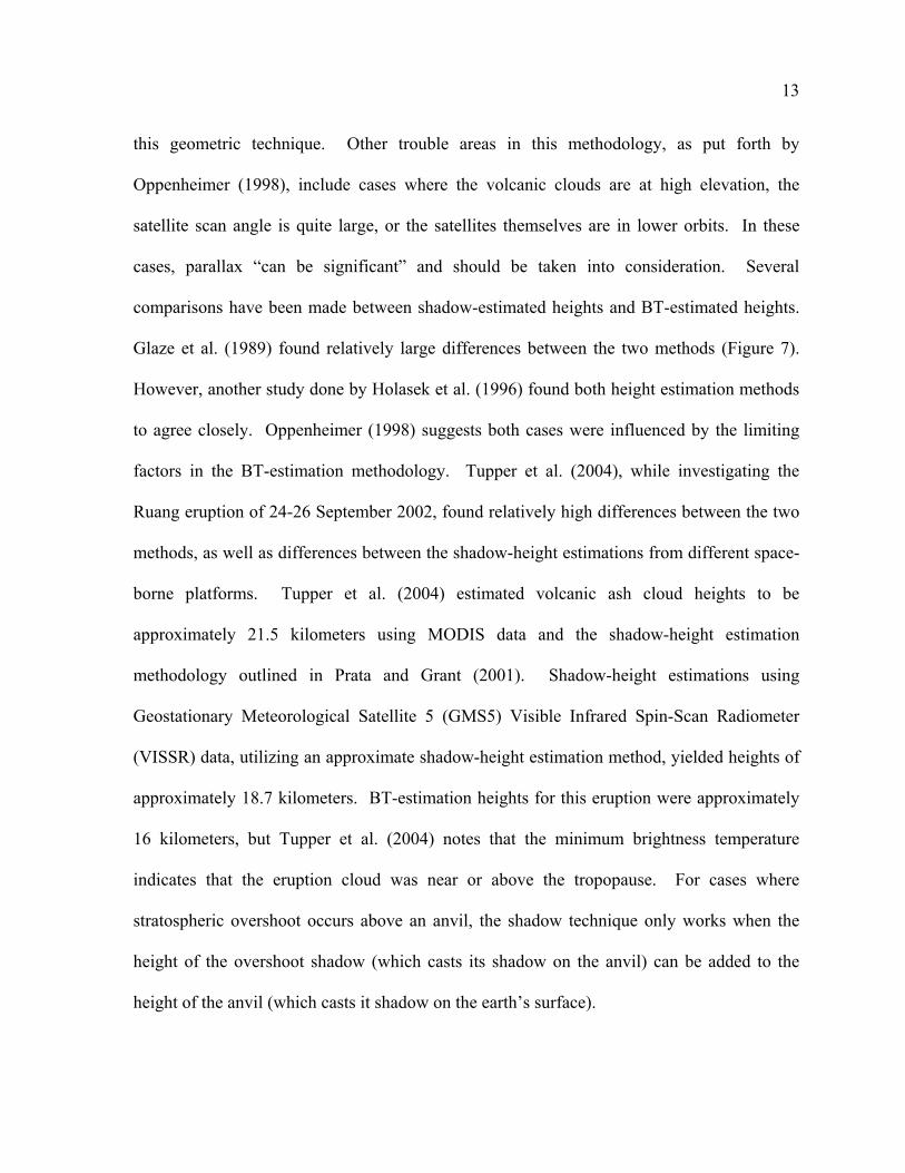
comparisons have been made between shadow-estimated heights and BT-estimated heights.

Glaze et al. (1989) found relatively large differences between the two methods (Figure 7).

However, another study done by Holasek et al. (1996) found both height estimation methods

to agree closely. Oppenheimer (1998) suggests both cases were influenced by the limiting

factors in the BT-estimation methodology. Tupper et al. (2004), while investigating the

Ruang eruption of 24-26 September 2002, found relatively high differences between the two

methods, as well as differences between the shadow-height estimations from different space-

borne platforms. Tupper et al. (2004) estimated volcanic ash cloud heights to be

approximately 21.5 kilometers using MODIS data and the shadow-height estimation

methodology outlined in Prata and Grant (2001). Shadow-height estimations using

Geostationary Meteorological Satellite 5 (GMS5) Visible Infrared Spin-Scan Radiometer

(VISSR) data, utilizing an approximate shadow-height estimation method, yielded heights of

approximately 18.7 kilometers. BT-estimation heights for this eruption were approximately

16 kilometers, but Tupper et al. (2004) notes that the minimum brightness temperature

indicates that the eruption cloud was near or above the tropopause. For cases where

stratospheric overshoot occurs above an anvil, the shadow technique only works when the

height of the overshoot shadow (which casts its shadow on the anvil) can be added to the

height of the anvil (which casts it shadow on the earth’s surface).

14

Figure 7. Heights retrieved by Glaze et al. (1989) for an eruption plume from the Lascar volcano (Chile) in 1986. Difference between heights retrieved by the BT-method and the shadow-method are approximately 4 kilometers. Error bars of 1.5 kilometers have been fitted to the shadow measurements. Image taken from Glaze et al. (1989).

Radar and lidar methods

Ground-based weather radar (Figure 8) has been used to detect the heights of volcanic ash

clouds (Lacasse et al., 2004; Tupper et al., 2004; Tupper et al., 2005). This study will not

discuss the specifics of the radar cloud height algorithm; for an extensive description of an

algorithm used to determine meteorological cloud heights using weather radar, the reader is

referred to Clothiaux et al. (2000). It is important, however, to note some of the limitations

15

of this method, as discussed in Tupper and Kinoshita (2003). Because ground radar stations

have limited range, the number of volcanic eruption clouds that pass within “reach” of a

ground-based weather radar is quite limited. Radar stations are quite expensive as well,

limiting the number of radar stations available worldwide. Radar estimates are also limited

by requiring the ash cloud to consist of certain particle sizes. Should an ash cloud consist of

only small particles, it may be invisible to weather radar. Also, heavy precipitation can

obscure radar height retrievals. Lidar, which measures the backscatter intensity of a laser

signal, has also been used to estimate volcanic cloud heights (Tupper et al., 2004).

Figure 8. Diagram illustrating radar scan of a volcanic eruption. Edited, original image taken from Lacasse et al. (2004).

Video and seismic methods

Additional methods for estimating ash cloud heights utilize video and seismic

instrumentation. Volcanic plume heights may be estimated using a geometric video

technique (e.g. Sparks and Wilson, 1982). In their investigation, Sparks and Wilson (1982)

use their calculated heights to assist in the estimation of other volcanic parameters including

particle content and volume discharge rate of magma. While they acknowledge errors can

16

occur when plumes stray from the vertical plane above the volcanic vent, they estimate that

dimensions estimated in their study are “better than 2 percent.” Volcanic ash plume heights

may also be estimated/forecast by analyzing volcanic tremor data (McNutt, 1994). McNutt

(1994) concludes that ‘explosivity of eruptions’, which is based on parameters such as ash-

column height, is proportional to the amplitude of volcanic tremor (normalized to a common

scale).

Pilot reports

Pilot reports (PIREPs) from commercial, general and military aircraft can be important

sources of ash cloud height information. They are also vital to the safety of all aviation as

PIREPs are often the first to inform of volcanic eruptions (Tupper and Kinoshita, 2003).

Unfortunately, PIREPs have been known to inaccurately report cloud top information and/or

be contradictory with other sources of data (Simpson et al., 2002; Tupper and Kinoshita,

2003; Tupper et. al., 2003). In general, pilot reporting is limited to daytime and good

visibility conditions (visibility immediately following an eruption might be quite poor).

17

IV. The Moderate Resolution Imaging Spectrometer (MODIS)

The Moderate Resolution Imaging Spectrometer (MODIS) (Figure 9) was developed for the

Terra and Aqua satellites of the National Aeronautics and Space Administration’s (NASA)

Earth Observing System (EOS). Soon after the successful launch of the Terra spacecraft on

December 18, 1999, MODIS began acquiring data, with its science data stream beginning on

February 24, 2000. A second MODIS instrument was launched with EOS’ Aqua platform on

May 4, 2002. Since this time, two MODIS instruments have observed the Earth, with each

instrument providing global coverage every two days (Platnick et al., 2003). The spectral

coverage, as well as the global spatial coverage that MODIS offers has yielded both new and

improved space borne remote sensing algorithms (e.g. King et al., 2003; Platnick et al, 2003;

Seemann et al., 2003). Although MODIS has a designed lifespan of approximately six years,

it is anticipated that the instruments will live much longer (Soulakellis et al., 2003). Only a

brief description of the MODIS instrument will be given here. For more complete

descriptions of MODIS and its products, the reader is referred to Ardanuy et al. (1991), King

et al. (1992), Barnes et al. (1998), and Platnick et al. (2003).

MODIS orbits the Earth in a near-polar, sun-synchronous orbit at an altitude of 705

kilometers. Terra is in descending orbit and has an equatorial crossing time of 1030 (local

solar time). Aqua is in an ascending orbit, with an equatorial crossing time of 1330 (local

solar time). This three-hour lag is advantageous in that it allows “characterization of diurnal

patterns” (Platnick et al., 2003). MODIS has an orbit period of ninety-nine minutes and

repeats its cycle every sixteen days.

18

Table 1. MODIS’ thrity-six spectral channels. Edited, original table taken from Barnes et al. (1998).

19

Figure 9. a) the MODIS instrument, courtesy of NASA; b) the area cut out by one MODIS granule over the continental United States (CONUS). Image courtesy of SSEC UW-Madison EOS Direct Broadcast; c) TERRA/MODIS orbit map and schedule for one 24-hour period (approximate). Image courtesy of NASA MODIS Rapid Response System & SSEC UW-Madison.

MODIS is a scanning radiometer that scans in “whiskbroom” fashion with a scan angle of

±55o. Its spectral capabilities consist of thirty-six unique channels, or “bands”, whose center-

20

frequencies range from approximately 0.415 to 14.235µm. Although the MODIS instrument

is capable of sub-kilometer spatial resolution at nadir, all but seven bands are at one-

kilometer resolution (at nadir). The two 250-meter channels, bands 1-2, are centered at 0.65

and 0.86µm, respectively, with the five 500-meter resolution channels, bands 3-7, centered at

0.47, 0.56, 1.24, 1.63, and 2.13µm, respectively. A listing of all thirty-six MODIS channels

is provided in Table 1. MODIS’ swath dimensions are 2330 kilometers (cross-track) by 10

kilometers (along-track), yielding ten, twenty, and forty along-track element arrays for the

1000-meter, 500-meter, and 250-meter bands, respectively (Platnick et al., 2003). MODIS

has a scan rate of 1.477 scans per second.

Numerous algorithms for cloud property retrievals have been developed for MODIS with

their products having relevance to many areas of atmospheric science. Such optical and

physical cloud properties include cloud-top pressure, cloud-top temperature, optical

thickness, and effective particle radius. MODIS cloud-top pressures are inferred by utilizing

the CO2-slicing methodology (Menzel et al, 1992), which takes advantage of the four

MODIS channels (bands 33-36) located within the 15µm CO2 absorption region as well as

the 11µm “atmospheric window” (band 31). The traditional MODIS cloud-top pressure

product has a spatial resolution of five kilometers at nadir. A description of the MODIS

CO2-slicing algorithm at 1000-meter resolution is presented in the next section.

21

V. CO2-slicing algorithm at 1000-meter resolution

Cloud top pressure may be inferred by application of the radiance-ratioing version of the

CO2-slicing technique (Wielicki and Coakley, 1981; Menzel et al., 1983; Wylie and Menzel,

1989; Baum and Wielicki, 1994; Wylie et al., 1994; McGarragh, 2004). The CO2-slicing

technique uses five infrared bands available on MODIS, with four of these bands located

within the 15µm CO2 absorption region (13.3µm – band 33; 13.6µm – band 34; 13.9µm –

band 35, and 14.2µm – band 36). The fifth infrared band is the 11µm window (band 31).

The CO2-slicing methodology takes advantage of the fact that the CO2 bands become more

transmissive with decreasing wavelength (Figure 10), i.e., as the bands move away from the

peak of the CO2 absorption at 15µm. This behavior is encapsulated by the peaks in the

weighting functions for these four CO2 bands (Figure 11), which are derived from the change

in transmission t with lnP in an atmospheric column. Three assumptions inherent in this

method are: 1) the clouds being observed are infinitesimally thick, 2) the surface emissivity

is that of a blackbody for the CO2 bands, and 3) that the cloud emissivity is identical in the

two bands being used (Menzel et al., 1983). We also make the assumption that scattering

may be neglected. For clouds above three kilometers above sea level (asl) (approximately

700hPa), cloud top pressures derived from the CO2-slicing method have accuracies to within

approximately ±50hPa (Menzel et al., 1983; Wylie and Menzel, 1989; Platnick et al., 2003,

Bedka et al., 2005) for many cases. The following description of the radiance-ratioing

version of the CO2-slicing technique closely follows Baum and Wielicki (1994) and

McGarragh (2004).

22

For a black surface (i.e. surface emissivity εs = 1), the clear-sky spectral radiance ICLR may be

given by

[ ] PdPdPdtPTBPtTBPI

ii

si

si

si

CLRPs

lnln

),ν()(,ν),ν(),ν(),ν(0

∫+= {4}

where B(νi, Ts) is the Planck radiance at temperature T (with subscript “s” denoting the

surface), νi is the wavenumber of band number i, and t(νi, P) is the transmittance from

atmospheric level P to the space-borne instrument at P = 0.

For a black cloud (i.e. cloud emissivity εc = 1) at pressure level Pc, the radiance IBLK may be

given by

[ ] PdPdPdtPTBPtTBPI

ii

ci

ci

ci

BLKPc

lnln

),ν()(,ν),ν(),ν(),ν(0

∫+= {5}

where the subscript “c” denotes the cloud.

For a single cloud layer in a single field of view (FOV), the top-of-the-atmosphere (TOA)

radiance I is given as

NIINI CLDCLR +−= )1( {6}

where N is the cloud fraction (the percentage of the FOV that contains cloud). ICLD is

expressed as

23

III BLKcCLRcCLD ε)ε1( +−= {7}

Substitution of Equation {7} into Equation {6} yields

ININI BLKcCLRc ε)ε1( +−= {8}

Equation {8} is an expression for the radiance from a partially cloudy FOV, and may be

rearranged to produce the “cloud signal” (I - ICLR).

)(ε IINII CLRBLKcCLR −=− {9}

We now substitute Equations {4} and {5} into Equation {9}, which, after further

simplification, yields

[ ]∫=−P

P

c

sPTdBPtNII ii

cii

CLR )(,ν),ν(ε)ν()ν( {10}

We now create a ratio of cloud signals for two different bands, dubbed the “G-function”,

where we introduce the superscript “j” as a second band number.

[ ][ ]∫

∫=

−−

=P

P

P

P

c

s

c

s

PTdBPt

PTdBPt

IIII

Pjj

ii

jjCLR

iiCLR

cijG

)(,ν),ν(

)(,ν),ν(

)ν()ν()ν()ν()( {11}

24

Figure 10. Transmittance from the top of the atmosphere to the surface for H2O, CO2, and O3, and for all three constituents combined. Calculated with LBLRTM 7.04 using the U.S. standard 1976 atmosphere. Image and caption taken from McGarragh (2004).

25

Figure 11. Weighting functions (dt/dlnp ) for five MODIS CO2 infrared bands as functions of pressure (mb). Calculated with the GDAS atmosphere for March 20, 2003 at 1200Z located on the equator at –30o longitude using a sensor view angle of 0o. Image and edited caption taken from McGarragh (2004).

We arrive at Equation {11} by making the assumption that both emissivities are equal for the

two closely spaced bands i and j (i.e. εci = εc

j). This assumption is the focus of research

presented later in this study.

The cloud signal ratio on the left side of Equation {11} is determined from radiances

measured by MODIS and the NOAA NCEP Global Data Assimilation System (GDAS)

gridded meteorological product, with the cloud signal ratio on the right side of {8} calculated

26

from a forward radiative transfer model (Menzel et al., 1983). The GDAS product provides

the temperature and water vapor mixing ratio data that is required to obtain the atmospheric

transmittance profiles. The temperature and water vapor mixing ratio data is provided at 16

separate pressure levels, however this data is extrapolated to 101 pressure levels, which is

required to calculate the transmittance profile. Also required to calculate the transmittance

profile is a 101-pressure level atmospheric ozone profile. This ozone profile is extrapolated

from LBLRTM model atmospheres. For a more complete description of the creation and

caching procedures of the transmittance profile, the reader is referred to the work of

McGarragh (2004). All CO2-slicing height retrievals presented in this study have been

derived from the GDAS profiles. It should be noted that true local atmospheric profiles

might differ significantly from the GDAS profiles used. Additional research must to be

conducted to determine how great an effect these potential discrepancies might have on the

CO2-slicing height product.

The G-function ratios are set up using pre-determined combinations of the four MODIS CO2

bands, as outlined in Platnick et al. (2003), with the addition of an additional band

combination (McGarragh, 2004). To summarize, the five band ratios used for this CO2-

slicing algorithm are band36/band35 (14.235µm/13.935µm), band36/band34

(14.235µm/13.635µm), band35/band34 (13.935µm/13.635µm), band35/band33

(13.935µm/13.335µm), and band34/band33 (13.635µm/13.335µm). For each band

combination, the cloud pressure Pc that best minimizes the difference between the observed

and calculated cloud signal (Equation {11}) is considered the most representative for that

pair. For the bands combinations outlined above, we will now be left with five representative

27

values for Pc. For each value of Pc, an “effective cloud amount” Nεc may be calculated by

rearranging Equation {9}.

)()()()(

εwIwI

wIwINCLRBLK

CLRc −

−=

{12}

where the w function dependence translates to radiances retrieved through the atmospheric

window channel (∼11µm). Due to MODIS’ 1000-meter resolution in the infrared region, the

effective cloud amount will be interpreted as cloud emissivity (McGarragh, 2004).

Following the work of Menzel et al. (1983), a final cloud-top pressure is chosen from the five

representative Pc values by error analysis.

[ ]∫−= −P

PccCLRik

ck

skk PTdBPtNIIM ii

i)(,ν),ν(εck)( {13}

∑ =

4

12

i kM i {14}

We use Equation {13} to check the difference between the cloud signal values and those

calculated from the radiative transfer equation. The subscripts “i” and “k” refer to the band

number (four in total) and representative Pc solution (five in total), respectively. The final

cloud-top pressure Pck is obtained when Equation {14} is a minimum. This final cloud top

pressure is converted to a height asl using the meteorological profiles in the GDAS product.

28

There are two situations that produce unacceptable retrievals (hereafter referred to as

“invalid” results) via the CO2-slicing method. The first considers the noise equivalent delta

radiance (NEDR) for the wavelength in question. A solution is considered invalid if either

cloud signal on the right-hand-side of Equation {11} falls within the NEDR for their

wavelength. The second refers to an issue regarding the interpolation of pressure levels, and

the reader is referred to McGarragh (2004) for a description of this limitation. In either case,

invalid CO2-slicing results are supplemented with heights obtained by using the BT-method

discussed in section III of this paper. This method is accomplished by interpolating the

11µm BTs into the atmospherically corrected BT profile, with the effective emissivity set to

unity. Height estimates at altitudes beneath the 700hPa pressure level are automatically

obtained using the BT-method, although, if desired, CO2-slicing results may be forced at

these altitudes. The forcing of the CO2-slicing method at altitudes lower than 700hPa does

not circumvent the NEDR limitation, however, as the BT-method will still be used for height

retrievals should the cloud-signal fall within the NEDR for their wavelength. Except where

noted, the results presented in this paper utilize the BT-method for altitudes beneath 700hPa.

There are several situations that are known to cause height retrieval errors with the CO2-

slicing methodology. The first, and perhaps the most significant when considering volcanic

eruptions, is the presence of temperature inversions in the atmosphere. The Pc solutions are

determined by the G-function (Equation {11}), which is a strongly dependant on the

atmospheric temperature profile. When a temperature inversion is present, the G-function

(Figure 12) inverts as well, creating two possible solutions (one above and one below the

inversion point). G-function retrieval problems also occur in isothermal regions of the

29

atmosphere. Surface temperature inversions and isothermal regions of the atmosphere are

more commonly present in polar atmospheres; therefore we limit our investigations in this

study to scenes located in tropical and mid-latitude atmospheres. One source of G-function

error that may be unavoidable, however, is the tropopause, where a temperature inversion is

always present. As will be shown in a later section, volcanic eruptions can pierce the

tropopause. The CO2-slicing algorithm begins by searching for the tropopause (the point

where the temperature begins to increase with decreasing height, moving downward from the

stratosphere). Should the tropopause be located at an altitude higher than the 100hPa

pressure level, the algorithm will assign the “tropopause” to be at 100hPa. In either case, the

“tropopause” assigns the maximum allowable G-function value (calculated). Should a cloud

lie in the isothermal layer, the observed G-function value might be greater than the maximum

G-function value allowed, in which case the pressure solution Pc is assigned according to the

maximum allowable G-function value. If a cloud lies near the tropopause, where the

observed G-function value corresponds to two different calculated G-function values (one

above and one below the physical tropopause), the higher pressure (lower height) is retained.

This assumption can lead to errors should a cloud pierce the tropopause, as the stratospheric

portions of the cloud would be assigned a height too low. If it is known that stratospheric

penetration has occurred, the algorithm may be forced to raise the “tropopause” well into the

stratosphere, and well above any physical cloud element that may be present. Should this be

done, stratospheric clouds would be assigned pressure values that correspond to the higher of

the two acceptable calculated G-function values (both now below the “tropopause”).

Tropospheric clouds near the physical tropopause, however, would be assigned heights too

high.

30

CO2-slicing can retrieve heights of stratospheric clouds if the clouds are known

independently to be located well above the isothermal layer. To retrieve these heights, a

separate version of the CO2-slicing algorithm that uses different interpolation logic must be

implemented. To retrieve the heights for a cloudy scene that contains both tropospheric and

stratospheric clouds, both the tropospheric and stratospheric versions of the CO2-slicing

algorithm must be run. Because the CO2-slicing methodology cannot distinguish between

these cloud types, the stratospheric version of the CO2-slicing algorithm may only be applied

to the cloudy regions otherwise known to contain stratospheric cloud elements. Unless

otherwise noted, all heights retrievals presented in this study were processed using the

tropospheric version of the CO2-slicing algorithm.

Figure 12. Cloud pressure function Gij(Pc) for (left) band ratio 34/33 calculated using tropical, mid-latitude, and polar profiles and for (right) band ratios 36/35, 36/34, 35/34, 35/33, and 34/33 calculated using a tropical profile. Calculated with the GDAS atmosphere for March 20, 2003 at 1200 using a sensor view angle of 0o. All atmospheres are located at –30o longitude with the tropical, mid-latitude, and polar atmospheres at 0o, 45o, and 90o latitude respectively. Image and caption taken from McGarragh (2004).

31

Menzel et al. (1992) and McGarragh (2004) also detail other potentially significant sources

of error that can arise from the assumptions made by the CO2-slicing algorithm. Two such

assumptions consider the surface properties that factor into the calculation of the clear-sky

spectral radiance, where the surface skin temperature is assumed to be the same as the

atmospheric temperature immediately above the surface, and surface emissivity is assumed to

be unity. Both assumptions can lead to error as warm and cold air advection and boundary

layer inversions can create drastic differences between the skin and surface air temperatures,

and surface emissivity is not always unity. These errors may be considered negligible

(McGarragh, 2004), however, if the MODIS CO2 band weighting functions (Figure 11) peak

above the surface.

Another assumption made by the CO2-slicing algorithm is that the clouds are infinitesimally

thick. This will lead to errors when observing optically thin clouds, as radiation originating

from within and below the cloud will be detected by the space-borne sensor (Menzel et al.,

1983). This, in-turn, leads the space-borne sensor to effectively “see” the thin clouds at

lower altitudes and underestimate the heights. As the clouds increase in optical thickness, the

“radiative center” of the clouds will increase in altitude, leading to more accurate height

assignments for the most optically thick clouds. There is, however, an overall low height

bias in CO2-slicing cloud height retrievals due to this assumption. For more detailed

descriptions of this limitation, the reader is referred to Smith and Platt (1978), Wielicki and

Coakley (1981), Menzel et al. (1983), and Menzel et al. (1992). Errors can also occurs can

also occur in the presence of multiple cloud layers. For complete descriptions of this

32

limitation and its error analysis, the reader is referred to Menzel et al. (1992), Baum and

Wielicki (1994), Frey et al. (1999), and McGarragh (2004).

The CO2-slicing height products presented in this paper do not consist entirely of fields of

view whose heights have been retrieved specifically by the CO2-slicing algorithm. Rather,

this paper presents the standard operational CO2-slicing product at 1000-meter resolution.

The standard product yields heights that are retrieved specifically by the CO2-slicing

algorithm, as well as the 11µm BT-method when the aforementioned limitations hinder the

application of the CO2-slicing algorithm. Although these results are presented as the “CO2-

slicing height product,” the reader should know that, except where noted, they may include

significant coverage by the 11µm BT-method.

VI. The Multi-angle Imaging SpectroRadiometer (MISR)

The Multi-angle Imaging SpectroRadiometer (MISR) was one of five instruments launched

December 18, 1999 aboard NASA’s Terra spacecraft. Built by the Jet Propulsion

Laboratory, MISR utilizes nine separate cameras that observe the earth in “pushbroom”

fashion in four spectral bands from Terra’s near-polar, sun-synchronous orbit. These nine

cameras “acquire moderately high-resolution imagery over a wide angular range in the along-

track direction” (Diner et al., 2002), with each camera viewing the earth at unique angles to

the local vertical (Figure 13). This unique nine-camera configuration allows MISR to

retrieve such cloud parameters as cloud-top heights using a “purely geometrical technique”

(Moroney, et al., 2002a). Provided here is a brief overview of the instrument and a

33

description of the cloud-top height retrieval methodology. A more complete description of

the MISR instrument may be found in Diner et al. (1998).

Figure 13. This graphic illustrates the measurement approach of the MISR instrument. Nine pushbroom cameras point at discrete angles along the spacecraft ground track, and data in four spectral bands are obtained for each camera. Image and caption taken from Diner et al. (2002).

The MISR instrument’s nine cameras (Table 2) are situated to provide a relatively large

angular range for along-track viewing. One camera is positioned at 0o (nadir, designated as

camera An), four cameras are pointed in the forward (along-track) direction, with the

remaining four cameras pointed in the aft direction. The four forward viewing cameras are

34

positioned at 26.1o (camera Af), 45.6o (camera Bf), 60.0o (camera Cf), and 70.5o (camera Df)

from nadir, with the aft viewing Aa, Ba, Ca, and Da cameras also positioned at 26.1o, 45.6o,

60.0o, and 70.5o from nadir, respectively. From Terra’s 705-kilometer orbit, MISR has an in-

nadir swath width of 376 kilometers and an off-nadir swath width of 413 kilometers, and the

time interval between a distinct point on the earth being viewed by the Df camera and the Da

cameras (the time it takes a point on the earth to be viewed by all nine MISR cameras) is

seven minutes (Diner et al., 2002). To account for the earth’s rotation during these seven

minutes, each camera’s cross-track angle is slightly offset (Diner et al., 1998), maximizing

the overlap by all cameras. The MISR instrument has a maximum resolution of 250 meters

at nadir, with a maximum off-nadir resolution of 275 meters. MISR views the entire Earth’s

surface in a period of nine days.

Table 2. MISR camera pointing requirements and as-built specifications. Table and caption taken from Diner et al. (1998).

35

Figure 14. Typical MISR camera configuration. Image courtesy of NASA (http://www-misr.jpl.nasa.gov/mission/mibigres.html)

Each of the nine MISR cameras consists of their own individual lens and is sensitive to four

unique spectral bands (Figure 14). The center wavelengths for these four bands are 446.3

(blue), 557.5 (green), 671.8 (red), and 866.5 (near-infrared) nanometers, and have widths of

40.9, 27.2, 20.4, and 38.6 nanometers, respectively (Bruegge, 1998). The wavelengths were

chosen for the MISR mission to avoid known regions of strong atmospheric gas absorption

and solar Fraunhofer lines. These wavelengths were also chosen for their applicability to

specific areas of research. The red and near-infrared wavelengths have applications to

marine aerosol studies (Kahn et al., 2001), while the green wavelength is very useful in

albedo studies (Jin et al, 2002).

36

VII. MISR height retrieval

The MISR cloud-top height product is produced using a stereophotogrammetric technique,

which, unlike the CO2-slicing methodology, does not require assuming any particular state of

the Earth’s atmosphere. The cloud-top height retrieval consists of two main steps, both of

which require the use of stereo-matching algorithms, which are described in detail in Diner et

al. (1999), Moroney et al. (2002a) and Muller et al. (2002). The first step involves retrieving

cloud-motion vectors (hereafter referred to as “wind”) and cloud-top height values at

relatively low resolution, with the second step being the cloud-top height retrieval at a higher

resolution. The “current operational processing” methodology will be briefly described and

details may be found in Moroney et al. (2002a). Analyses from early on in MISR’s

operational life suggest cloud-top heights to be accurate to within ±562 meters at 1.1-

kilometer resolution (Moroney et al., 2002a).

In truth, cloud-top heights may be retrieved without utilizing the aforementioned first step.

However, any cloud motion due to advection during the seven minute time interval required

for all nine MISR cameras to view a specific scene may lead to significant errors. The wind

correction process utilizes three cameras and pairs them as Bf-Df and Bf-An (Figure 15). The

use of three cameras allows for solutions from the stereo-matching algorithm to be achieved

for both wind and cloud-top height simultaneously. These retrievals are made at a coarse

70.4-kilometer resolution. The winds are then decomposed into their north-south and east-

west components and are binned in a two-dimensional histogram. For each 70.4-kilometer

domain, the modal value of the histogram is considered its representative wind field.

37

Additionally, all winds must pass a quality test. Error analysis suggests wind speed errors of

±3 m/s, corresponding to heights errors (from these winds) of ±400 meters (Moroney et al.,

2002a).

Figure 15. MISR viewing geometry for the An and Bf cameras. Image and caption taken from Moroney et al. (2002b).

The second step in the MISR cloud-top height retrieval method first consists of dividing the

70.4-kilometer domain into smaller, 1.1-kilometer sub-region. Considering the previously

calculated wind correction values (identical for each 1.1-km sub-region within a 70.4-km

domain), the stereo-matching algorithm is run twice in each sub-region to obtain cloud-top

height values, once for the Af-An camera pair and once for the Aa-An camera pair. While the

data ingested by the stereo-matching algorithm is at 275-kilometer resolution, time

restrictions require cloud-top height values to be retrieved for every fourth pixel (1.1-

kilometer resolution). In each sub-region, the stereo-matching algorithm may not find a valid

38

match within the allowable search window. If only one camera pair retrieves a valid match,

the height is accepted. If both camera pairs return valid matches and both resultant heights

agree within a certain threshold, the higher of the two heights is retained. This threshold is

described in detail in Diner et al. (1999), but may be summarized by

σN hσ-h][meanh

∆•∆≥∆ {15}

σN hσh][meanh

∆•+∆≥∆ {16}

where ∆h is the difference between the two heights, [mean∆h] is the mean of the height

differences for all points in the domain containing the pixel in question, σ∆h is the standard

deviation for this distribution, and Nσ is a configurable parameter (Diner et al., 1999). If

both Equation {15} and {16} prove true, both heights are considered to agree within the

threshold. If the two heights do not agree, both are rejected. One limitation to the height

algorithm occurs in the presence of multi-layered clouds. Multi-layered cloudy scenes have

been known to cause confusion for the stereo-matching algorithms and are known problem

areas for MISR’s cloud-top height retrieval method. A recent investigation published in

Naud et al. (2004) concludes “Optically thin clouds were found to be accurately

characterized by the MISR cloud-top height product as long as no other cloud was present at

a lower altitude.” A more detailed description of the limitations to MISR’s cloud-top height

retrieval methodology may be found in Moroney et al. (2002a).

39

The final cloud-top height product can be viewed in several ways. The two main ways the

height products are the “Best Winds” and “Without Winds”. Without Winds simply means

that there was no wind correction applied in the two-step height retrieval process. This view

does not yield the “true” height field (unless the real wind speed was uniformly zero), but

rather gives an “overview” of the heights in the scene. Best Winds yield the “best guess” as

to the true height field. Because wind retrievals of good quality only occur 55-60% of the

time (Catherine Moroney, personal communication 2005), Best Wind views might not yield

the entire height field.

There have been studies published in which MISR’s height product is compared with both

the operational MODIS CO2-slicing algorithm (Moroney et al., 2002a) and lidar data (Naud

et al., 2004). In the MISR comparison, a TERRA overpass was collocated in time and space

with reflectivities retrieved from a 94-GHz ground-based radar. This study found heights to

be in MODIS heights to be in agreement with the radar to ±1.5 kilometers, while MISR

heights were in agreement to ±500 meters. In the lidar comparison, one year of back-

scattering lidar cloud boundaries and optical depth were compared with MISR. MISR was

found to differ with the lidar from –0.1 and 0.4 kilometers for low clouds and from 0.1 and

3.1 kilometers for high clouds.

40

VIII. CO2-slicing heights compared with MISR heights

For the MODIS/MISR comparisons presented in this section, we utilize two different

versions of the MISR height product. The first version of the MISR height algorithm is a

product of the production code publicly available at the time of this investigation, and we

hereafter refer to this MISR algorithm version as version alpha. The second version of the

MISR height algorithm is a product of a prototype height algorithm (hereafter referred to as

version beta) that has been specially run for this investigation by Catherine Moroney of the

MISR science team. The beta height algorithm contains two main improvements to version

alpha. The first improvement is a more accurate wind calculation algorithm. The second

improvement is better wind quality control measures, as the winds in the beta version are

calculated separately for the forward- and aft- viewing cameras, which are then compared.

Because of these improved wind quality flags, coverage in the “best winds” version of the

beta MISR height algorithm might be significantly decreased. The new wind calculations are

now believed to be more accurate (Catherine Moroney – personal communication 2005),

which will improve the “best winds” height retrievals. The beta version of the MISR height

algorithm is, as yet, not public, however it is slated to become operational by late 2005.

To facilitate pixel-to-pixel comparisons for MODIS’ 1.0-kilometer resolution and MISR’s

1.1-kilometer resolution height products, a special collocation algorithm was required. The

MODIS/MISR collocation algorithm used in this investigation was written by and is

provided courtesy of Michael Garay of the Jet Propulsion Laboratory in Pasadena, California,

41

USA. This algorithm regrids the MODIS and MISR data to a third grid of lower resolution,

allowing 100 percent coverage of both instruments’ height products.

In this section, we compare CO2-slicing height retrievals with MISR’s stereo heights for four

volcanic plumes (Table 3). All MISR data presented in this section is of format number 7

and software version 11 or higher. The statistics for these comparisons (Table 4) were

generated after collocation of the MODIS and MISR data. Following the collocation, a

section of each volcanic plume known to have coverage with MISR’s alpha version best

winds height product was isolated. These sections were isolated by bounding them in a

latitude/longitude box; the boxes’ corner points are printed in Table 3. The corner points

were determined so as to also eliminate contamination by meteorological cloud and

erroneous height retrievals from the earth’s surface. Trimmed-means (middle 80%) were

calculated from the bounded, collocated pixels.

The following analysis concerns only the best wind heights retrieved by MISR by both the

alpha and beta versions. The without winds height product is presented as a reference to the

coverage that MISR did have for each individual plume, however, its height product should

not be considered representative of the plumes’ heights without knowledge of the true local

wind field. In addition, the CO2-slicing height product utilizes the 11µm BT-method to

estimate heights for fields of view where the CO2-slicing algorithm fails. Should noise levels

become too high, the 11µm method may, at times, be applied to the entire MODIS granule.

42

Anatahan

24 May 2003

The Anatahan Volcano is located in the Pacific Ocean 320 kilometers north of Guam and

approximately 120 kilometers north of Saipan Island. Its first historical eruption was on 10

May 2003 (US Geological Survey – 2005). Volcanic activity continued during the following

weeks, and TERRA’s instruments captured one of Anatahan’s volcanic plumes on 24 May

2004 (Figure 16). For the area of the volcanic plume selected for analysis (Table 3), both

MODIS (panel “b”) and MISR’s alpha algorithm (panels “d”) agree that the height of this

plume was 2000 meters ± 300 meters. MISR’s beta algorithm, however, suggests that the

heights might have been higher. The beta best winds product presents a trimmed-mean value

close to 5000 meters, with a standard deviation (sd) of zero meters. Graphical inspection of

the entire plume for this product (panel “f”), however, shows that the beta best wind product

did, in fact, yield heights that were less than 3000 meters for parts of the plume. The

discontinuity in the height field is representative of discontinuities in the MISR retrieved

wind field. For the plume’s selected region, however, MISR’s beta best winds suggests

much higher heights than both the MODIS and MISR alpha algorithm products, although the

drastic discontinuity in the wind field causes some lack of confidence in this bounded

region’s height retrieval.

43

Figure 16. Eruption of the Anatahan Volcano, 24 May 2003, 0055Z, observed by TERRA. a) MODIS true color image; b) MODIS CO2-slicing height product; c) MISR alpha version “without winds” height product; d) MISR alpha version “best winds” height product; e) MISR beta version “without winds” height product; f) MISR beta version “best winds” height product.

Chikurachki

22 April 2003

The Chikurachki Volcano is located on Paramushir Island in the northern Kurile Islands,

Russia. MODIS and MISR captured an ash plume from Chikurachki on 22 April 2003

44

(Figure 17). MISR’s alpha height product retrieved a trimmed-mean height of 2038 meters

and the MODIS CO2-slicing algorithm retrieved a trimmed mean height of 878 meters, with

standard deviations of 604 meters and 475 meters, respectively. MISR’s beta algorithm

again yielded higher heights with a trimmed-mean height of 3210 meters (252 sd). There

were, however, only 12 pixels considered for the MISR beta best wind algorithm. Panel “f”

shows the drastic lack of coverage for this plume in the MISR beta height product.

Figure 17. Eruption of the Chikurachki Volcano, 22 April 2003, 0054Z, observed by TERRA. a) MODIS true color image; b) MODIS CO2-slicing height product; c) MISR alpha version “without winds” height product; d) MISR alpha version “best winds” height product; e) MISR beta version “without winds” height product; f) MISR beta version “best winds” height product.

45

Etna

29 October 2002

Mount Etna is located on the island of Sicily in Italy at 37.73oN and 15.0oE. MODIS and

MISR height retrievals for the volcanic plume captured on 19 October 2002 (Figure 18) are

in relative disagreement. MODIS CO2-slicing yields a trimmed-mean height of 2161 meters,

with an sd of 1833 meters. MISR’s alpha and beta algorithms yield trimmed-mean heights

of 4354 meters (1527 meters sd) and 3610 meters (2128 meters sd), respectively. Although

MISR’s beta algorithm does not retrieve much of Etna’s plume, the trimmed data contains

731 points.

Manam

29 November 2004

The Manam Volcano is described in detail in Section IX of this study. On 29 November

2004, a low-level plume from Manam (Figure 19) was captured by MODIS and MISR. The

CO2-slicing and MISR alpha trimmed-means for the selected volcanic domain are again in

disagreement with trimmed-mean heights of 866 meters (356 meters sd) and 2154 meters

(1490 meters sd), respectively. It is clear from panels “d” and “f” that the MISR coverage

for the volcanic plumes in the best winds product is lacking. This was definitely taken into

account when determining the plume region selected for this plume’s statistics.

Unfortunately, MISR’s beta height algorithm didn’t retrieve any heights for this plume as

seen in panel “f”. Although 48 pixels from this algorithm were found in the collocated third

46

grid, these pixels may have been extrapolated from anomalous surface retrievals and are not

being considered in this analysis.

Figure 18. Eruption of the Etna Volcano, 29 October 2002, 0945Z, observed by TERRA. a) MODIS true color image; b) MODIS CO2-slicing height product; c) MISR alpha version “without winds” height product; d) MISR alpha version “best winds” height product; e) MISR beta version “without winds” height product; f) MISR beta version “best winds” height product.

47

Figure 19. Eruption of the Manam Volcano, 29 November 2004, 0040Z, observed by TERRA. a) MODIS true color image; b) MODIS CO2-slicing height product; c) MISR alpha version “without winds” height product; d) MISR alpha version “best winds” height product; e) MISR beta version “without winds” height product; f) MISR beta version “best winds” height product. CO2-slicing heights for this scene have been forced down to 1000mb.

48

Table 3. Details on volcanic cases investigated for MODIS/MISR height retrieval comparison.

Volcano

Date

MODISscan time

MISR

orbit#/blocks

Lat/Lon

box* Anatahan 24 May

2003 0055Z 18242/77-79 lats: 16.0 / 15.25

lons: 145.9 / 145.8 Chikurachki 22 April

2003 0045Z 17776/49-51 lats: 50.25 / 50.0

lons: 156.0 / 155.75 Etna 22 July

2001 0955Z 08476/61-63 lats: 37.5 / 36.5

lons: 16.0 / 15.25 Etna%,1 27 October

2002 1000Z 15204/61-63 lats: 37.4 / 37.0

lons: 15.1 / 15.0 Etna%,2 27 October

2002 1000Z 15204/61-63 lats: 35.75 / 34.75

lons: 14.75 / 14.25 Etna 29 October

2002 0945Z 15233/60-62 lats: 37.0 / 36.5

lons: 15.5 / 15.25 Manam 29 November

2004 0040Z 26324/93-95 lats: -3.62 / -3.8

lons: 146.5 / 146.25 * Corners for latitude/longitude box that encapsulates the pixels used for the MODIS/MISR

comparison. These corners were chosen so as to capture only volcanic pixels. % This case refers to data plotted in Figure 22. 1 Region 1 for this plume 2 Region 2 for this plume

Figure 20 is a graphical representation of the data presented in Table 4. An alternative

MODIS/MISR comparison is presented in Figure 22. This plot presents an additional two

volcanic cases to the four already analyzed in this section. The additional two volcanic cases

(Figure 21 – two separate regions) were not previously analyzed because, while they were

‘collocatable’ with the collocation algorithm, the plume region could not be segregated. This

code issue is under investigation. The trimmed-mean heights presented in Figure 22 are not

results from collocated data as in Figure 20. Figure 22 presents statistics from the segregated

plume sections (as listed in Table 3) without collocation. Because MISR’s height product is

49

at a slightly higher resolution than MODIS’, the number of pixels investigated for MISR will

be less. Statistics for the MISR data come from MISR’s alpha best winds height retrievals.

The small discrepancies for these products’ statistics between Figure 20 and Figure 22 are

assumed to stem from the lower-resolution third grid used for the collocation.

Table 4. Comparison of MODIS CO2-slicing and MISR height retrievals. Data is the trimmed-mean (middle 80%) for all heights retrieved in lat/lon box (in meters). Numbers in parentheses indicate number of pixels (from neutral third grid) used in retrieval. Numbers in brackets are the standard deviation for the trimmed data (in meters).

Eruption

MODIS

CO2-slicing*

MISR alpha

“without winds”

MISR alpha “best

winds”

MISR beta

“without winds”

MISR beta “best

winds”

Anatahan

1732.6 (1538)

[257.0]

2127.3 (1538)

[263.0]

2247.3 (1538)

[243.3]

2354.2 (1523)

[419.0]

4980.5 (917) [0.0]

Chikurachki

877.6 (720)

[475.1]

2061.5 (550)

[500.2]

2037.9 (561)

[604.2]

2087.7 (482)

[442.7]

3209.6 (12)

[252.1]

Etna1

2161.0 (2057)

[1833.1]

4364.2 (1413)

[1601.3]

4354.3 (1317)

[1526.6]

4274.3 (1330)

[1723.5]

3609.7 (731)

[2127.9]

Manam

865.9 (779)

[356.3]

3691.3 (877)

[1482.8]

2154.3 (753)

[1490.4]

3300.9 (760)

[1524.4]

n/a2

* 11µm brightness temperature method is applied on fields of view where CO2-slicing fails (see text for description).1 Etna eruption on 29 October 2002 2 data believed invalid; see description in text

50

Figure 20. MODIS and MISR trimmed mean heights (middle 80%) for four volcanic eruptions after collocation. Plots representative of data in Table 4. Plots bounded in a black box refer to MISR’s alpha height algorithm, non-black-box-bounded plots refer to MISR’s beta height algorithm.

51

Figure 21. Eruption of the Etna Volcano, 27 October 2002, 1000Z, observed by TERRA. a) MODIS true color image; b) MODIS CO2-slicing height product; c) MISR alpha “without winds” height product; d) MISR alpha “best winds” height product; e) MISR beta “without winds” height product; f) MISR beta “best winds” height product.

52

Figure 22. MODIS and MISR trimmed mean heights (middle 80%) for six volcanic eruptions without collocation. Whiskers on each plot represent the standard deviation for the trimmed data.

53

IX. CO2-slicing heights compared with operational height estimation methods

Manam

The Manam volcano is located 12 kilometers north of Papua New Guinea at latitude 4.1S and

longitude 141.06E. The Manam volcano is measured to be 1807 meters high. Numerous

eruptions occurred at Manam between October 2004 and January 2005. These eruptions

have been documented meteorologists, including those at the Darwin Volcanic Ash Advisory

Centre (VAAC), Australia. The following analyses of the Manam eruptions are based on

personal correspondence with Andrew Tupper (senior meteorologist – Darwin VAAC).

24 October 2004

The eruption of the Manam Volcano on 24 October 2004 was observed by MODIS (from

both AQUA and TERRA) (Figure 23). Panels “b”, “d” and “e” show the CO2-slicing height

products for 0105Z, 0355Z and 1620Z, respectively. The 0105Z height product indicates that

the eruption plume disperses from the vent in two distinct sections. The first section travels

to the northwest at a lower altitude then the other plume, eventually descending to a height

indicated by CO2-slicing to be below 3000 meters. The second plume section is the updraft

column, which at this time has reached a CO2-slicing retrieved height of 16.8km. The 0355Z

MODIS imagery reveals that the updraft column had begun to drift to the north and expand,

almost completely shielding the lower plume from view by the MODIS instrument on

AQUA. CO2-slicing heights put this higher cloud also at 16.8km. The 1620Z MODIS image

shows that the CO2-slicing technique has retrieved the heights for a volcanic ash cloud

(enclosed in red circle) that is over twelve hours old. Maximum heights here are near

54

Figure 23. Eruption of Manam Volcano, 24 October 2004. a) MODIS [TERRA] true color image at 0105Z; b) MODIS [TERRA] CO2-slicing height product at 0105Z; c) MODIS [AQUA] true color image at 0355Z; d) MODIS [AQUA] CO2-slicing height product at 0355Z; e) MODIS [AQUA] CO2-slicing height product at 1620Z, ash region circled in red.

16.4km. The heights retrieved for the three MODIS scans suggest that the volcanic cloud

approached or entered the tropopause (defined using the GDAS profile used in the CO2-

slicing retrieval). Because CO2-slicing cannot retrieve heights very near an isothermal

region, maximum heights for this eruption are estimated to be between 16.5km and 17.0km.

55

The lowest infrared BTs for this eruption are –69oC, which, according to local radiosonde

data, places the cloud below the tropopause. The local radiosonde data, taken from Momote

(approximately 348km northeast of Manam), at 00Z 24 October 2004 indicates the

tropopause is near a height of 17.8km (Appendix A). Forward trajectories, however, indicate

a height assignment of 18.5km might be more appropriate. Final operational estimates for

this eruption cloud’s height are 17-18.5km (Andrew Tupper – personal communication

2005). CO2-slicing’s height retrievals when compared to the operational estimates are within

±50hPa.

31 October 2004

CO2-slicing heights for the 31 October 2004 eruption of the Manam Volcano are illustrated

in Figure 24. The highest height value retrieved by CO2-slicing in this eruption cloud is near

16.8km, presumably very near the tropopause region. An atmospheric sounding from

Momote at 00Z, about one hour prior to the MODIS overpass, put the tropopause at

approximately 16.4km. Darwin VAAC estimates for the height of this eruption cloud were

made using shadow height and the BT method. The shadow height estimation method

suggested height greater than 15.0km, while infrared cloud top brightness temperatures of

approximately -80oC put cloud top height near the 16.4km high tropopause. Final

operational height estimates for this cloud are 16-16.5km (Andrew Tupper – personal

communication 2005) with a final CO2-slicing height estimate of 16.5-17.0km.

56

Figure 24. Eruption of Manam Volcano, 31 October 2004, 0110Z, observed by TERRA. a) MODIS true color image; b) MODIS CO2-slicing height product for the troposphere at 1km resolution. True color image courtesy of the Darwin VAAC.

57

Figure 25. Eruption of Manam Volcano, 19 December 2004. a) MODIS [TERRA] 11µm image at 1235Z; b) MODIS [TERRA] CO2-slicing height product at 1235Z; c) MODIS [AQUA] 11µm image at 1530Z; d) MODIS [AQUA] CO2-slicing height product at 1530Z.

19 December 2004

The eruption of the Manam volcano on 19 December 2004 was captured twice by MODIS

(Figure 25). Panels “c” and “d” show a well-defined plume extending east-southeast from

the vent. CO2-slicing height retrievals for the 1530Z MODIS scan yield maximum ash cloud

heights near 16.7km. This case is quite similar to the 24 October 2004 and 31 October 2004

58

Manam cases as the highest parts of this cloud are believed to be at or in the tropopause

region (where CO2-slicing will retrieve a height coinciding with the coldest GDAS altitude).

CO2-slicing suggest maximum heights of 16.5-17.0km for this eruption scene. Minimum

brightness temperatures of –80oC from the 1530Z MODIS image, compared with a Momote

radiosonde at 00Z on 20 December 2004 (Appendix B), put operational height estimates also

at 16.5-17.0km.

27 January 2005

CO2-slicing heights were also retrieved for the Manam eruption of 27 January 2005 (Figure

26). The center portions of this cloud were stratospheric (panel “c”, green arrow) with an

overshooting, ‘undercooled’ top of –71oC, with a total stratospheric overshoot of 19o-22oC.

The tropospheric version of the CO2-slicing algorithm (panel “b”) is not able to identify the

stratospheric portions of the cloud as being above the tropopause and places heights near

12km. Because this portion of the cloud is independently known to be stratospheric, the

stratospheric version of the CO2-slicing algorithm may be applied to this case. CO2-slicing

yields maximum heights of 22-23km for the stratospheric cloud that had not been

‘undercooled.’ These height estimates correspond very well with operational estimates from

the temperature data, which put the coldest stratospheric portions (-63oC) in a height range of

21-24km. This height range was determined from radiosonde data from Momote at 00Z on

27 January 2005 (Appendix C).

59

Figure 26. Eruption of Manam Volcano, 27 January 2005, 1535Z, observed by AQUA. a) MODIS 11µm image; b) MODIS CO2-slicing height product for the troposphere; c) MODIS CO2-slicing product for stratosphere. The majority of the volcanic cloud has been ‘blacked out’ to highlight the stratospheric cloud height retrievals. 11µm image courtesy of Darwin VAAC.

60

Miyakejima

18-19 August 2000

Mount Oyama is located on the Japanese island of Miyake-Jima at latitude 34.08oN and

longitude 139.52oE, and it has a height of 818.7 meters. Tupper et al. (2004) investigated

this eruption (Figure 27) and, using wind-correlation methods, estimates that the ash cloud

Figure 27. Eruption cloud from Miyakejima Volcano, 19 August 2000, 0105Z, observed by TERRA. a) MODIS true color image; b) MODIS CO2-slicing height product, eruption cloud circled in red.

61

identified in panel “b” is at a height of 5-8km. CO2-slicing height retrievals average at a

lower altitude, with most cloud elements assigned heights of 3-6km. Maximum CO2-slicing

heights (6.5km) appear in the center of the cloud, where optical thickness is greatest. These

height retrievals are a good match to the operational estimates (Andrew Tupper – personal

communication 2005), however CO2-slicing does appear to underestimate the heights in the

optically thinner regions.

Ruang

25 September 2002

The Ruang Volcano is located at latitude 2.28oN and longitude 125.425oE in the Sangihe

Islands of Indonesia. Its height is measured at 725 meters. MODIS passes at 0450Z and

1415Z on 25 September 2002 retrieved heights for volcanic clouds from Ruang (Figure 28).

AQUA’s pass at 0450Z captured the eruption cloud soon after it had pierced the stratosphere.

Tupper et al. (2004) indicates that the highest heights retrieved operationally for this eruption

were 21.5km by shadow method applied to MODIS. When all other height estimation

techniques were considered, Tupper et al. (2004) arrived at a final height estimate of

20±2km. Because portions of this cloud are believed to be stratospheric, the stratospheric

version of the CO2-slicing methodology was applied to the 0450Z MODIS scan (panel “b”,

green arrow). CO2-slicing technique yielded heights up to 21.2km for this scene. This height

retrieval is in very good agreement with the operational estimates. Agreement with

operational estimates for the CO2-height retrievals from the 1415Z TERRA pass (panel “d”)

was not as strong, however. Cloud “D” found in panel “c” was estimated to be between 16-

18km through operational methods (Tupper et al., 2004) while CO2-slicing retrieved heights

62

around 9±1km. The 16-18km operational estimate is made with high confidence (Andrew

Tupper – personal communication 2005) and it is possible that MODIS missed the high cloud

completely due to the cloud’s low optical depth. The 9±1km heights may actually be

retrievals from another cloud at a lower altitude.

Figure 28. Eruption clouds from Ruang Volcano, 25 September 2002: a) MODIS [AQUA] CO2-slicing height product for the troposphere at 0450Z; b) MODIS [AQUA] CO2-slicing height product for the stratosphere at 0450Z. The majority of the volcanic cloud has been ‘blacked out’ to highlight the stratospheric cloud height retrievals; c) Image highlighting volcanic clouds for the TERRA 1415Z pass, colored regions highlight ash clouds with high confidence; d) MODIS [TERRA] CO2-slicing height product at 1415Z. Image in panel “c” taken from Tupper et al. (2004).

63

Table 5. CO2-slicing height estimates compared with operational estimates for volcanic eruptions. Except where noted, ‘Times after eruptions’ is the time after the initial volcanic eruption and are approximate.

Volcano

Date

MODIS time(s) (UTC)

Time after

eruption

CO2-slicing height

estimate*

Operational height

estimate#

Manam

24 October 2004

0105, 0355,

& 1620

3 hours%

16.5km –

17km

17km – 18.5km

(BT/wind)

Manam

31 October

2004

0110

16 hours

16.5km –

17km

16km – 16.5km (BT/shadow)

Manam

19 December

2004

1235

& 1530

12 hours$

16.5km –

17km

16.5km – 17km

(BT)

Manam

27 January

2005

1535

1.5 hours

22km – 23km

21km – 24km

(BT)

Miyakejima

19 August

2000

0105

17 hours1

3km – 6km, max ~6.5km

5km – 8km 1

(wind)

Ruang 25

September 2002

0450

70 min1

max

~21.2km

20±2km1

(shadow/others)

Ruang

25 September

2002

1415

10.5

hours1

9±1km2

16km – 18km1,2

(?)

Sheveluch

21 May 2001

0120

7 hours4

3km – 9km, max ~12km

max heights 6.7km & 4.9km3

(BT) * 11µm brightness temperature method is applied on fields of view where CO2-slicing fails (see text for description). # Operational estimates courtesy Darwin/VAAC except where noted. Operational method(s) used in parenthesis. % Corresponding to 0105Z MODIS pass $ Time after intensification of eruption that began at 00Z 18 December 2004; corresponds to

1235Z MODIS pass 1 Tupper et al. (2004) 2 Estimation for cloud “D” in Figure 28, panel “c”. 3 Operational estimates courtesy Tokyo/VAAC, see text for explanation. 4 Kamchatkan Volcanic Eruptions Response Team (KVERT) – via Tokyo VAAC

64

Sheveluch

20-21 May 2001

The Sheveluch Volcano (Figures 30 and 31) is located on the Kamchatka Peninsula in Russia

at a latitude/longitude of 55.38oN/161.19oE with a summit height of 24447 meters. A

TERRA pass on 21 May 2001 at 0120Z allowed MODIS to capture an eruption plume from

Sheveluch. The height retrievals from this pass are presented in Figure 29, with the

maximum CO2-slicing heights approaching 12km, however most of the volcanic pixels

seems to range from 3-9km. BT analysis performed by the Tokyo VAAC on products from

the Japanese Geostationary Meteorological Satellite (GMS) estimate ash top heights at

approximately 6.7km and 4.9km for 2132Z on 20 May 2001 and 0232Z on 21 May 2001,

respectively (Yasuhiro Kamada/Tokyo VAAC – personal communication 2005). Yasuhiro

Kamada does suggest, however, that if these volcanic clouds were semi-transparent, the BT-

method heights would be under-estimates.

Figure 29. MODIS [TERRA] CO2-slicing height product for eruption plume from the Sheveluch Volcano at 0120Z on 21 May 2001.

65

X. CO2-slicing heights compared with heights estimated by video and photographic techniques

In this section, volcanic ash cloud heights produced by the CO2-slicing methodology are

compared to height estimates made by video and photographic and techniques. The volcanic

eruptions presented here (Figure 32) occurred at the Sheveluch Volcano, and were chosen

based on their recognizable plume signature. The video and photo height estimation

techniques described here have been taken from Senyukov et al. (2004 – unpublished data)

and personal correspondence with Sergey Senyukov (Research Laboratory of Seismic and

Volcanic Activity, Kamchatkan Experimental-Methodical Seismological Department).

Video and photo imagery used for plume height analysis for the Sheveluch Volcano were

made from the “Kluchi” seismic station (Figure 30). The volcano profile has been scaled

using well-known altitudes of local features (Figure 31). For height estimates, each video or

photographic image is rescaled to this volcano profile, allowing each eruption cloud to be

measured by the same altitude scale. Senyukov et al. (data not yet published) indicates that

there is error in the linear scale of the volcano profile. This error, however, which has been

estimated to be 2% at 3 kilometer elevation, 3% at 10 kilometer elevation, and 5% at 15

kilometer elevation, is considerably less than errors that may arise from “deviation of the ash

column from the vertical line.” Senyukov et al. (2004 – unpublished data) also describes a

method where volcanic plumes heights from Sheveluch are estimated using a purely seismic

technique, and these results are compared to the photographic and video estimates. Results

from this seismic method will not be presented in this study. The CO2-slicing method has

been forced down to 1000hPa for the cases shown here.

66

Figure 30. Map of the Kamchatka Penninsula, Russia and the Sheveluch volcano and its vicinity. Seismic station “Kluchi” is indicated by a triangular symbol. Image taken from Senyukov et al. (2004 – unpublished data).

Figure 31. Sheveluch ash plume on 28 August 2000 at 2235Z with volcano profile overlaid on image. Photo by Yury Demyanchuk. Image taken from Senyukov et al. (2004 – unpublished data).

67

CO2-slicing heights were retrieved for a MODIS pass at 0030Z on 23 August 2000 (panel

“a”). This scan captured a volcanic plume from Sheveluch that has maximum retrieved

heights near 16.2km. Approximately forty-five minutes prior to the MODIS pass, the

video/photo technique estimates the ash column to be 17.5km high. A suggested error for

this video/photo estimate is –42.86% and a possible source of this error is deviation of the

eruption column from the vertical plain.

MODIS captured an eruption plume from Sheveluch at 2355Z on 28 August 2000 (panel

“b”). Maximum CO2-slicing heights for this plume are near 10.2km. About one and one half

hour before this height retrieval, video/photo techniques estimated this eruption column to

have a height of 16.5km. A suggested error for this video/photo estimate is –66.67%, again

associated with the deviation of the eruption column from the vertical plain. This eruption is

depicted in Figure 31.

At 0000Z on 27 August 2003, MODIS captured an eruption plume (panel “c”) that has

maximum CO2-slicing retrieved heights of near 3.8km. Estimates made by video/photo

techniques at 0021Z, twenty-one minutes after the MODIS pass, place the eruption plume

height at 3.5km.

68

Figure 32. a) MODIS [TERRA] CO2-slicing height products for Sheveluch eruptions. CO2-slicing heights have been forced down to 1000hPa. a) 23 August 2000, 0030Z; b) 28 August 2000, 2355Z; c) 27 August 2003, 0000Z.

Table 6. CO2-slicing height estimates compared with video/photo method estimations for Sheveluch Volcano

Date

Time(s) (UTC)

CO2-slicing height estimate*

Video/photo height estimate#

23 August 2000

0030

16.2km

17.5km1

28 August 2000

2355

10.2km

16.5km2

27 August 2003

0000

3.8km

3.5km3

* 11µm brightness temperature method is applied on fields of view where CO2-slicing fails (see text for description).

# Video/photo estimates courtesy of Sergey Senyukov 1 Approximately 45 minutes prior to CO2-slicing estimate 2 Approximately 90 minutes prior to CO2-slicing estimate 3 Approximately 21 minutes after CO2-slicing estimate

69

XI. Changes to the CO2-slicing methodology in consideration of volcanic ash

The CO2-slicing methodology is implemented with the assumption that cloud emissivities of

the two spectral bands are equal. This assumption, however, may lead to errors in height

retrievals. Zhang and Menzel (2002) investigated potential improvements to the cloud and

surface emissivity assignments in the CO2-slicing algorithm. Their study, which focused on

high, thin cirrus clouds, found appropriate emissivity corrections that adjusted the cloud-top

pressure retrievals for high, thin cirrus up to 10-20hPa (with root mean square bias

differences of approximately 50hPa). In our study, we investigate potential adjustments to

the cloud emissivity ratio in the CO2-slicing algorithm in consideration of volcanic ash. The

results presented here are not to be taken as necessary adjustments that should be

implemented for volcanic ash clouds. Additional research, as well as a rigorous validation

process, must be performed to establish new operational emissivity ratios. Rather, we

provide these results to explore if this approach of including volcanic emissivity corrections

to the CO2-slicing algorithm would be useful.

The CO2-slicing algorithm is based on a ratio of cloud signals for two closely spaced spectral

bands (Equation {11} in section V). This ratio is built from the cloud-signals that are defined

by Equation {10}. These ratios consist of a cloud fraction and a wavelength dependent cloud

emissivity that may ‘cancel’ out with creation of Equation {11}. Neglecting the wavelength

specific cloud emissivities is only possible if we consider them to be equal. If we do not

make this assumption, the G-function would then become

70

[ ]

[ ]∫

∫=

−−

=PP

PTvdBPvtc

PP

PTvdBPvtc

vIvIvIvI

Pc

s

c

s

jjj

iii

jCLR

j

iCLR

i

cijG

)(,),(

)(,),(

)()()()()(εε

{17}

where all symbols are as they were before except for εci and εc

j, which correspond to the

cloud emissivity for wavelengths i and j, respectively. New height retrievals may now be

conducted by the method described in section V.

Wavelength specific emissivities for volcanic ash are determined from the single scatter

properties of the andesite mineral, which is a common model for “volcanic ash” (e.g. Yu et

al, 2002; Pavolonis et al., 2005). The single scatter properties of andesite were determined

by applying Mie calculations to assumed particle size distributions (containing only spherical

particles) using the method outlined in Pavolonis et al. (2005). Asymmetry parameter, single

scatter albedo, and the extinction (βext) and absorption (βsca) coefficients were generated for

five specific effective radii (0.33µm, 1.63µm, 2.41µm, 4.39µm, and 8.1µm) for each CO2

band, where the effective radius for the size distribution is defined as the third moment over

the second moment. Using these CO2 band- and effective radius-dependent single scatter

properties, βeff is then approximated by substitution into Equation {18} (Parol et al., 1991):

ββ

ωgωωgω

)1)(1(

)1)(1(

abs

absj

i

ijj

jii

eff −−

−−≈β

{18}

71

where ω is the single scatter albedo, g is the asymmetry parameter, βabs = βext – βsca is the

absorption coefficient, and βeff is given in Giraud et al. (1997) by:

[ ]εεβ

ci

ceffj

−−= 11 {19}

The cloud emissivity ratios used by the CO2-slicing algorithm are plotted in Figure 33 for the

five effective radii.

Although there have been investigations into the physical size of ash particles from eruption

plumes, due to the great variability of ash particle size from eruption to eruption, as well

variability within the plumes themselves, βeff is approximated (red dashed lines, Figure 33).

By setting βeff = εci / εc

j, we approximate the cloud emissivity ratio correction for band ratio

14.235µm/13.935µm to 1.07, and we approximate the corrections for band pairs

14.235µm/13.635µm, 13.935µm/13.635µm, 13.935µm/13.335µm, and 13.635µm/13.335µm

to 0.93. Figure 34 presents a plot of Equation {19} for εci / εc

j vs. εci for βeff = 1.07 (green)

and βeff = 0.93 (blue). Figure 34 indicates that these βeff = εci / εc

j approximations are

appropriate for thinner volcanic ash (emissivity < ~0.6) as the adjusted emissivity corrections

βeff approximate the emissivity ratios better than the assumed ratio value of unity.

CO2-slicing height retrievals have been run using the 1.07 and 0.93 emissivity correction

factors for fifteen volcanic plumes presented in this study, and the results are presented in

Figure 34 and Table 7. Figure 34 is a graphical representation of the pixel-by-pixel height

changes that occurred for each of the volcanic plumes with the correction of cloud

72

emissivities. Table 7 presents resultant height corrections in tabular form. The cloud

emissivity corrections do not affect fields of view where the 11µm BT height retrieval

method is used. Only pixels whose height was retrieved specifically by the CO2-slicing

algorithm are presented in these results. While the majority of volcanic plumes investigated

in this study were almost entirely retrieved by the CO2-slicing algorithm, several cases were

limited to the 11µm method and are not presented here. In addition, several plumes (e.g.

Chikurachki; Etna 27 Oct.) were retrieved partially by the CO2-algorithm, and the height

correction statistics for these cases do not reflect changes to the entire plumes.

Figure 33. Cloud emissivity ratio plotted as a function of effective radius. Ratio corrections are indicated by the dashed red lines.

73

It should be noted that the MODIS trimmed-mean heights for several eruption clouds

presented in Table 7 differ significantly from the MODIS trimmed-mean heights presented in

Table 3 for the same clouds. The results presented in this section consider only pixels whose

height was retrieved specifically by the CO2-slicing algorithm, whereas the MODIS/MISR

comparisons consider all pixels (either CO2-slicing or 11µm method). The difference in

means suggests that there were fields if view in the isolated lat/lon domains that were

retrieved via the 11µm method, and that these fields of view were large in number compared

to the number of fields of view retrieved by the CO2-slicing algorithm and/or the fields of

view retrieved by the 11µm method were significantly lower in heights than those retrieved

by the CO2-slicing algorithm.

Application of the 1.07 and 0.93 emissivity corrections causes an increase in the CO2-slicing

retrieved heights for all but one volcanic plume. For the fourteen plumes where the heights

increased, the average increase is 870.5 meters. The average change to the heights for all

cases with the emissivity correction is +755.4 meters. The height change for each plume was

determined by calculating the difference between the pre- and post-adjusted trimmed-mean

heights (pre-adjusted subtracted from post-adjusted). The trimmed-mean heights are mean

values for the middle 80 percent of the individual plume data; the upper and lower 10 percent

is not considered in order to prevent statistical contamination by outlying height values. The

volcanic plumes we investigated reside in a variety of atmospheres and at differing altitudes.

We applied the emissivity correction to two stratospheric cases: 1) Manam, 27 January 2005,

1535Z and 2) Ruang, 25 September 2002, 0450Z). While the application of the 1.07 and

74

0.93 emissivity correction increased the heights for the Ruang stratospheric ash cloud, it

lowered the heights for the Manam ash cloud (Figure 34, panel “j”) by 856.6 meters.

Figure 34. εci / εc

j vs. εci for βeff = 1.07 (green) and βeff = 0.93 (blue) from Equation

{19}. Red dashed lines indicate emissivity correction of 1.07 and 0.93.

75

Figure 35. Height corrections to volcanic plumes from adjusted cloud emissivity ratios. Positive numbers indicate height increased with adjusted cloud emissivity ratios. a) Chikurachki, 22 April 2003, 0045Z; b) Etna, 27 October 2002, 1000Z; c) Etna, 29 October 2002, 0945Z; d) Manam, 24 October 2004, 0105Z; e) Manam, 24 October 2004, 0355Z; f) Manam, 24 October 2004,1620Z; g) Manam, 31 October 2004, 0110Z; h) Manam 19 December 2004, 1235Z; i) Manam, 19 December 2004, 1530Z; j) Manam, 27 January 2005, 1535Z; k) Ruang, 25 September 2002, 0450Z; l) Ruang, 25 September 2002, 1415Z; m) Sheveluch, 23 August 2000, 0030Z; n) Sheveluch, 28 August 2000, 2355Z; o) Sheveluch, 21 May 2001, 0120Z.

76

Table 7. CO2-slicing height adjustments for volcanic ash plumes* in consideration of calculated cloud emissivity corrections

Volcano

Date

Time (UTC)

Pixels1

Trimmed-

mean height2

Adjusted trimmed-

mean height3

Height

change4

Chikurachki 22 April 2003

0045 35 6431.5 7625.0 1193.5

Etna 27 October 2002

1000 140 4905.8 6017.0 1111.2

Etna 29 October 2002

0945 323 5409.5 6308.5 899.0

Manam 24 October 2004

0105 271 11375.0 11984.3 609.3

Manam 24 October 2004

0355 14062 14475.1 15437.7 962.6

Manam 24 October 2004

1620 7842 14835.4 16445.1 1609.7

Manam 31 October 2004

0110 244 15532.4 16008.1 475.7

Manam 19 December 2004

1235 659 9002.0 9476.2 474.2

Manam 19 December 2004

1530 158 16457.1 16598.0 140.9

Manam 27 January 2005

1535 1828 20015.2 19158.6 -856.6

Ruang

25 September

2002

0450

120

18668.5

19370.0

701.5

Ruang

25 September

2002

1415

2776

8895.5

9834.9

939.4

Sheveluch 23 August 2000

0030 661 12746.1 13970.6 1224.5

Sheveluch 28 August 2000

2355 1397 8409.4 8779.0 369.6

Sheveluch 21 May 2001

0120 37 8228.3 9704.8 1476.5

*Minor contamination by meteorological cloud is possible, though unlikely. 1 The number of pixels investigated for each plume. The same pixels were used for both the ‘trimmed-mean height’ and the ‘adjusted trimmed-mean height.’ These pixels have been designated as “volcanic.” 2 The trimmed-mean height (middle 80% - in meters) for the volcanic pixels before the emissivity correction was applied. 3 The trimmed-mean height (middle 80% - in meters) for the volcanic pixels after the emissivity correction was applied 4 The height correction, calculated by [‘trimmed-mean height’ subtracted from ‘adjusted trimmed-mean height’] (in meters)

77

XII. Conclusions and Future Work

This study compares the MODIS CO2-slicing height product with heights retrieved from

various other methods, including stereo height retrieval algorithms of MISR, flown on the

same satellite. CO2-slicing height estimations are also compared with operational height

estimation techniques such as the 11µm brightness temperature technique, wind correlation

methods, and a shadow technique, as well estimations made from a video/photo method. The

CO2-slicing height product is presented as a combination of the CO2-slicing and 11µm height

estimation products. For fields of view where the CO2-slicing algorithm cannot be

performed, height retrievals are supplemented via the 11µm brightness temperature method.

Pixel-to-pixel comparisons of the MODIS and MISR height products (Table 4) reveal that

the CO2-slicing product consistently retrieves lower heights than MISR for volcanic ash. For

the cases presented in Table 4, MODIS does not come within 500 meters of either MISR

height retrieval algorithm version. For the other three cases, MODIS does not come within

1000 meters of either MISR height retrieval algorithm version. An alternative

MODIS/MISR height product comparison (Figure 22) reveals similar results with MODIS

always retrieving lower height for volcanic ash. Figures 20 and 22 show that all six volcanic

ash comparisons indicate MODIS to be lower than MISR. These volcanic ash plumes,

however, are at relatively low altitudes, and the CO2-slicing algorithm is not known to be

accurate at altitudes below 700hPa. Figure 22 also indicates that the variability of these

methods’ height retrievals for these eruption are quite similar.

78

The CO2-slicing height product is compared with operational techniques (e.g. 11µm BT-

method, shadow technique, wind correlation methods) used professionally by meteorologists

(Table 5). The CO2-slicing height product compared well with the estimates made by the

operational techniques for the majority of these cases. These volcanic plumes were at much

higher altitudes overall than the MISR cases, with all but two residing near the tropopause or

in the lower stratosphere. For the two stratospheric cases (Manam, 27 January 2005; Ruang,

25 September 2002 at 0450Z), the CO2-slicing results fell squarely inside the three to four

kilometer height window estimated by the operational techniques. Similar results are

obtained for the tropopause cases (Manam, 24 October 2004; Manam, 31 October 2004;

Manam, 19 December 2004; Ruang, 25 September 2002 at 1415Z), where the CO2-slicing

height product falls within ±50hPa of the operational estimate (Manam 31 October and 19

December were within ±25hPa) for three of the cases. In the fourth case (Ruang, 25

September 2002 at 1415Z), CO2-slicing apparently misses the ‘tropopausal’ volcanic ash

cloud completely and retrieves the height of an underlying cloud. CO2-slicing estimates for

the mid-troposphere also fall within the operation estimate windows, however their

agreement is not as strong. For the vast majority of the Miyakejima volcanic cloud, the CO2-

slicing height estimates fall below the operational height estimates. Only the believed-to-be

optically thick maxima produce height results that are high enough to fall within the

operational estimate window. CO2-slicing height results from Sheveluch 21 May 2001 vary

too greatly to enable establishment of an official CO2-slicing height estimate.

The CO2-slicing height product is also compared with height estimates of volcanic plumes

from the Sheveluch Volcano made by a video/photo technique (Table 6). The CO2-slicing

79

heights estimates for two of the cases compare well with the video/photo estimates. The first

of these cases is a volcanic ash cloud near the tropopause (23 August 2000), where CO2-

slicing estimates the cloud to be 1.3 kilometers lower than the video/photo estimate made 45

minutes before. The second case is a lower-altitude plume (27 August 2003) where CO2-

slicing estimates 300 meters above the video/photo technique estimate made 21 minutes

later. A third video/photo comparison shows CO2-slicing falling well below the video/photo

estimate. The video/photo technique estimated the height of the 28 August 2000 Sheveluch

plume to be at a height of 16.5 kilometers. This estimate is 90 minutes after the MODIS

overpass, where CO2-slicing retrieved maximum heights of 10.2 kilometers.

The comparisons presented in this study suggest that improvements could be made to the

MODIS CO2-slicing methodology to improve its retrieval of volcanic ash cloud heights.

While CO2-slicing is seen to perform quite well for many cases (often the higher-altitude

cases), the methodology often underestimates the height of airborne volcanic ash. Two

situations where volcanic ash might be underestimated have been revealed in this study:

• The MODIS/MISR comparisons suggest that the CO2-slicing height product might

underestimate the height of low-level volcanic ash clouds. The cases investigated in

this study were all retrieved by MODIS to be below 3000 meters, however MISR

identified several of these clouds to be much higher (4–6 kilometers).

• Comparisons with operational techniques suggest that optically thin volcanic ash

clouds might be a problem area for the CO2-slicing methodology. The Miyakejima

volcanic cloud (Figure 27) was an optically thin cloud around the edges, with regions

of optically thick cloud in the middle (Andrew Tupper – personal communication

80

2005); the CO2-slicing height retrievals varied accordingly. Evidence of a possible

optical thickness limitation can be seen in the 28 August 2000 Sheveluch plume

(Figure 32, panel “b”). The MODIS height retrieval was made 90 minutes after the

video/photo estimate, which gave the higher ash particles time to descend to lower

altitudes. While the video/photo technique saw the fine particles at the higher

altitude, MODIS saw “through” them, retrieving heights from thicker cloud lying

beneath. This perceived limitation is a topic for future research that is not restricted

to volcanic ash clouds; it has applicability to cloud-top-pressure height retrievals for

meteorological clouds.

An area of potential improvement to the CO2-slicing algorithm is the cloud emissivity ratio

assumption. For CO2-slicing, the standard assumption is that the cloud emissivities for two

spectrally close channels are the same (i.e. the cloud emissivity ratio is unity). This study

investigated potential changes that could be made to this cloud emissivity assumption in

consideration of volcanic ash. We arrived at cloud emissivity ratios that may be applied to

volcanic ash clouds as first corrections to the standard cloud emissivity assumptions. Using

cloud emissivity corrections of 1.07 (band combinations 36/35) and 0.93 (band combinations

36/34, 35/34, 35/33, and 34/33), MODIS CO2-slicing height retrievals increased an average

of 755.4 meters for fifteen volcanic ash cloud cases (Table 7). Only one of the fifteen cases

investigated cases saw a decrease in heights with these emissivity corrections.

This is the first known investigation into the role CO2-slicing might play in retrieving the

heights of volcanic ash clouds. It is difficult to validate the height retrievals and thus where

81

improvement needs to be made. The comparisons chosen for this study were based on their

differing methodologies. While MISR is a space-borne instrument, it retrieves cloud heights

by a stereophotogrammetric technique. The operational techniques were chosen due to their

continued use amongst the scientists and meteorologists tracking volcanic ash clouds

operationally in real- and near real-time. Additional future research aimed at determining

CO2-slicing’s applicability to real- or near real-time estimation of volcanic ash cloud heights

will need to focus on the cloud and surface emissivity assumptions inherent in the CO2-

slicing methodology. Emissivity adjustments in consideration of volcanic ash will likely

differ from adjustments made for meteorological clouds. A necessary additional component

to CO2-slicing comparisons with other height estimation methods is an examination of the

CO2-slicing product itself. Cloud emissivity corrections will not affect height retrievals

made by the 11µm BT-method. An investigation into the situations where CO2-slicing fails

and where the 11µm method is applied for volcanic ash clouds is appropriate. This will assist

in determining appropriate adjustments to the CO2-slicing algorithm.

82

XIII. References

Ardanuy, P. A., Han, D., and Salomonson, V. V., (1991) The Moderate Resolution Imaging Spectrometer (MODIS) science and data system requirements. IEEE Transactions on Geoscience and Remote Sensing, 29, 75–88. Barnes, W. L., Pagano, T. S., and Salomonson, V. V. (1998) Prelaunch characteristics of the “Moderate Resolution Imaging Spectroradiometer (MODIS) on EOS-AM1. IEEE Transactions on Geoscience and Remote Sensing, 36, 1088–1100. Baum, B. A. and Wielicki, B. A. (1994) Cirrus cloud retrieval using infrared sounding data: Multilevel cloud errors. Journal of Applied Meteorology, 33, 107-117. Bedka, S. T., Feltz, W. F., Schreiner, A. J., and Holz, R. E. Satellite derived cloud top pressure product validation using aircraft based cloud physics lidar data from the AtREC field campaign. International Journal of Remote Sensing - accepted for publication. Bruegge, C. J., Duval, V. G., Chrien, N. L., Korechoff, R. P., Gaitley, B. J., and Hochberg, E. B. (1998) MISR prelaunch instrument calibration and characterization results. IEEE Transactions on Geoscience and Remote Sensing, 36, 1186-1198. Casadevall, T. J. (1994). The 1989-1990 eruption of Redoubt Volcano, Alaska: impacts on aircraft operations. Journal of Volcanology and Geothermal Research, 62, 301-316. Casadevall, T. J. and M. D. Krohn (1995). Effects of the 1992 Crater Peak eruptions on airports and aviation operations in the United States and Canada. U.S. Geological Survey Bulletin 2139, 205-220. Casadevall, T. J., Delos Reyes, P. J., and Schneider, D. J. (1996) The 1991 Pinatubo eruptions and their effects on aircraft operations, in Fire and Mud: eruptions and lahars of Mount Pinatubo, Philippines. Edited by C. G. Newhall and R. S. Punongbayan, pp. 637-645, Philippines, Institute of Volcanology and Seismology & University of Washington Press, Quezon City & Seattle. Clothiaux, E. E., Ackerman, T. P., Mace, G. G., Moran, K. P., Marchand, R. T., Miller, M. A., and Martner, B. E. (2000) Objective determination of cloud heights and radar reflectivities using a combination of active remote sensors at the ARM CART sites. Journal of Applied Meteorology, 39, 645-665. Diner D. J., Beckert, J. C., Reilly, T. H., Bruegge, C. J., Conel, J. E., Kahn, R. A., Martonchik, J. V., Ackerman, T. P., Davies, R., Gerstl, S. A. W., Gordon, H. R., Muller, J., Myneni, R. B., Sellers, P J., Pinty, B., and Verstraete, M. M. (1998) Multi-angle Imaging SpectroRadiometer (MISR) instrument description and experiment overview. IEEE Transactions on Geoscience and Remote Sensing, 36, 1072-1087.

83

Diner, D. J., Davies, R., DiGirolamo, L., Horvath, A., Moroney, C., Muller, J. -P., Paradise, S., Wenkert, D., and Zong, J. (1999) MISR level 2 cloud detection and classification algorithm theoretical basis document. Jet Propulsion Laboratory (JPL), California Institute of Technology, Pasadena, CA, JPL Technical Document D-11399. Diner, D. J., Beckert, J. C., Bothwell, G. W., and Rodriguez, J. I. (2002) Performance of the MISR instrument during its first 20 months in orbit. IEEE Transactions on Geoscience and Remote Sensing, 40, 1449-1466. Dunn, M. G. and Wade, D. P. (1994) Influence of Volcanic Ash Clouds on Gas Turbine Engines, in Volcanic Ash and Aviation Safety - Proceedings of the First International Symposium on Volcanic Ash and Aviation Safety. Edited by T. J. Casadevall, U.S. Geological Survey Bulletin 2047, 107-118. Frey, R. A., Baum, B. A., Menzel, W. P., Ackerman, S. A., Moeller, C. C., and Spinhirne, J. D. (1999) Validation of CO2-slicing cloud heights computed from MAS radiance data during SUCCESS. Journal of Geophysical Research, 104(D20), 24,547-24,555. Giraud, V., Buriez, J. C., Fouquart, Y., Parol, F., and Seze, G. (1997) Large-scale analysis of cirrus clouds from AVHRR data: Assessment of both a microphysical index and the cloud-top temperature. Journal of Applied Meteorology, 36, 664-675. Glaze, L. S., Francis, P. W., Self, S., and Rothery, D. A. (1989) The 16th September 1986 eruption of Lascar volcano, north Chile: satellite investigations. Bulletin of Volcanology, 51, 149-160. Grindle, T. J. and F. W. Burcham (2002) Even minor volcanic ash encounters can cause major damage to aircraft. ICAO journal, 57, 12-14, 29. Holasek, R. E., Self, S., and Woods, A. W. (1996) Satellite observations and interpretation of the 1991 Mount Pinatubo eruption plumes. Journal of Geophysical Research, 100, 8469-8487. Jin, Y., Gao, F., Shaaf, C. B., Li, X., Strahler, A. H., Bruegge, C. J., and Martonchik, J. V. (2002) Improving MODIS surface BRDF/albedo retrieval with MISR multiangle observations. IEEE Transactions on Geoscience and Remote Sensing, 40,1593-1604. Johnson, R. W. and T. J. Casadevall (1994) Aviation safety and volcanic ash clouds in the Indonesia-Australia region. U.S. Geological Survey Bulletin 2047, 191-197. Kahn, R., Banerjee, P., McDonald, D., and Martonchik, J. (2001) Aerosol properties derived from aircraft multiangle imaging over Monterey Bay. Journal of Geophysical Research, 106 (D16), 11977-11995.

84

King, M. D., Kaufman, Y. J., Menzel, W. P., and Tanré, D. (1992) Remote sensing of cloud, aerosol, and water vapor properties from the Moderate Resolution Imaging Spectrometer (MODIS). IEEE Transactions on Geoscience and Remote Sensing, 30, 2–27. King, M. D., Menzel, W. P., Kaufman, Y. J., Tanre, D., Gao, B. –C., Platnick, S., Ackerman, S. A., Remer, L. A., Pincus, R., and Hubanks, P. A. (2003) Cloud and aerosol and water vapor properties, precipitable water, and profiles of temperature and humidity from MODIS. IEEE Transactions Geoscience and Remote Sensing, 41, 442-458. Lacasse, C., Karlsdottir, S., Larsen, G., Soosalu, H., Rose, W. I., and Ernst, G. G. J. (2004) Weather radar observations of the Hekla 2000 eruption cloud, Iceland. Bulletin of Volcanology, 66, 457-473. Lynch, J. S., and Stephens, G. (1996) Mount Pinatubo: A satellite perspective of the June 1991 eruption, in Fire and Mud: eruptions and lahars of Mount Pinatubo, Philippines. Edited by C. G. Newhall and R. S. Punongbayan, pp. 637-645, Philippines, Institute of Volcanology and Seismology & University of Washington Press, Quezon City & Seattle. McGarragh, G. (2004) The effect of multilayered clouds on cloud pressure retrievals in near-global MODIS data. [Masters Thesis] Department of Atmospheric and Oceanic Sciences, University of Wisconsin-Madison, Madison, Wisconsin, USA. McNutt, S. R. (1994) Volcanic tremor amplitude correlated with eruption explosivity and its potential use in determining ash hazards to aviation, in Volcanic ash and aviation safety: proceedings of the First international symposium on Volcanic ash and aviation safety. Edited by T. J. Casadevall. U.S. Geological Survey Bulletin B 2047, 377-385. Menzel, W. P., Smith, W. L., and Stewart, T. R. (1983) Improved cloud motion wind vector and altitude assignment using VAS. Journal of Applied Meteorology, 22, 377-384. Menzel, W. P., Wylie, D. P., and Strabala, K. I. (1992) Seasonal and diurnal changes in cirrus clouds as seen in four years of observations with the VAS. Journal of Applied Meteorology, 31, 370-385. Moroney, C., Davies, R., and Muller, J. (2002a) Operational retrieval of cloud-top heights using MISR data. IEEE Transactions on Geoscience and Remote Sensing, 40, 1532-1540. Moroney, C., Horvath, A., and Davies, R. (2002b). Use of stereo-matching to coregister multiangle data from MISR. IEEE Transactions on Geoscience and Remote Sensing, 40, 1541-1546. Muller, J. –P., Mandanayake, A., Moroney, C., Davies, R., Diner, D. J., and Paradise S. (2002) MISR stereoscopic image matchers: Techniques and results. IEEE Transactions on Geoscience and Remote Sensing, 40, 1547-1559.

85

Naud, C., Muller, J. –P., Haeffelin, M., Morille, Y., and Delaval, A. (2004) Assessment of MISR and MODIS cloud top heights through inter-comparison with a back-scattering lidar at SIRTA. Geophysical Research Letters, 31, L04114, doi:10.1029/2003GL018976. Oppenheimer, C. (1998) Volcanological applications of meteorological satellites. International Journal of Remote Sensing, 10, 2829-2864. Parol, F., Buriez, J. C., Brogniez, G., and Fouquart, Y. (1991) Information content of AVHRR Channels 4 and 5 with respect to the effective radius of cirrus cloud properties. Journal of Applied Meteorology, 30, 973-984. Pavolonis, M. J., Feltz, W. F., Heidinger, A. K., andGallina, G. M. (2005) A daytime compliment to the reverse absorption technique for improved automated detection of volcanic ash. Submitted to Journal of Oceanic and Atmospheric Technology. Platnick, S., King, M. D., Ackerman, S. A., Menzel, W. P., Baum, B. A., Riédi, J. C., and Frey, R. A. (2003) The MODIS Cloud Products: Algorithms and Examples from Terra. IEEE Transactions on Geoscience and Remote Sensing, 41, 459-473. Prata, A. J. (1989a) Observations of volcanic ash clouds using AVHRR-2 radiances. International Journal of Remote Sensing, 10 (4-5), 751-761. Prata, A. J. (1989b) Radiative transfer calculations for volcanic ash clouds. Geophysical Research Letters, 16 (11), 1293-1296. Prata, A. J., Bluth, G., Rose, B., Schneider, D., and Tupper, A. (2001) Comments on “Failures in detecting volcanic ash from a satellite-based technique”. Remote Sensing of Environment, 78, 341-346. Prata, A. J.and Grant, I. F. (2001) Determination of mass loadings and plume heights of volcanic clouds from satellite data. CSIRO Technical Paper 48, CSIRO Dept. of Atmospheric Science, Melbourne, Australia, 39 pp Rose, W. I., Bluth, G. J. S., and Ernst, G. G. J. (2000) Integrating retrievals of volcanic cloud characteristics from satellite remote sensors: A summary. Philosophical Transactions of the Royal Society of London, A, 358, 1585-1606. Rossier, R. N. (2002, February) Volcanic Ash: Avoid at all costs. Business and Commercial Aviation, 70-71. Sawada, Y. (1987) Study on analysis of volcanic eruptions based on eruption cloud image data obtained by the Geostationary Meteorological Satellite (GMS). Meteorology Research Institute (Japan), Tokyo, 335 pp.

86

Seemann, S., Li, J., Menzel, W. P., and Gumley, L. (2003) Operational Retrieval of Atmospheric Temperature, Moisture, and Ozone from MODIS Infrared Radiances. Journal of Applied Meteorology, 42, 1072-1091. Senyukov, S. L., Droznin, D. V., and Droznina, S. Ya. (2004 – unpublished data) The ongoing eruption of Sheveluch Volcano (Kamchatka Peninsula, Russia): Remote determination of ash plume initiation and height using local seismicity. Kamchatkan Experimental-Methodical Seismological Department GS RAS. Simpson, J. J., Hufford G., Pieri D., and Berg, J. (2000a) Failures in detecting volcanic ash from a satellite-based technique. Remote Sensing of Environment, 72, 191-217. Simpson, J. J., McIntire, T., Jin, Z., and Stitt, J. R. (2000b) Improved cloud top height retrieval under arbitrary viewing and illumination conditions using AVHRR data. Remote Sensing of the Environment, 72, 95-110. Simpson, J. J., Hufford, G. L., Pieri, D., Servranckx, R., Berg, J. S., and Bauer, C. (2002) The February 2001 eruption of Mt. Cleveland, Alaska: a case study of an aviation hazard. Weather and Forecasting, 17, 691-704. Smith, W. L., and Platt, C. M. R. (1978) Comparison of satellite-deduced cloud heights with indications from radiosonde and ground-based laser measurements. Journal of Applied Meteorology, 17, 1796-1802. Soulakellis, N., Yates, J., and Tataris, G. (2003) Global Island Image-Maps (GIIM): A set of digitally processed MODIS images. International Cartographic Association 2003 Conference. Durban, South Africa. Sparks, R. J. S. and Wilson, L. (1982) Explosive volcanic eruptions – V. Observations of plume dynamics during the 1979 Soufrière eruption, St Vincent. Geophysical Journal of the Royal Astronomical Society, 69, 551-570. Tupper, A. S., and Kinoshita, K. (2003) Satellite, air and ground observations of volcanic clouds over islands of the southwest Pacific. South Pacific Study, 23, 21-46. Tupper, A., Kinoshita, K., Kanagaki, C., Iino, N., and Kamada, Y. (2003) Observations of volcanic cloud heights and ash-atmosphere interactions. WMO/ICAO Third International Workshop on Volcanic Ash, Toulouse, France, September 29 -October 3, 2003. Tupper, A., Carn, S., Davey, J., Kamada, Y., Potts, R., Prata, F., and Tokuno, M. (2004) An evaluation of volcanic cloud detection techniques during recent significant eruptions in the western ‘Ring of Fire’. Remote Sensing of Environment, 91, 27-46.

87

Tupper, A., Oswalt, J. S., and Rosenfeld, D. (2005) Satellite and radar analysis of the volcanic-cumulonimbi at Mount Pinatubo, Philippines, 1991. Journal of Geophysical Research, 110(D09204): doi:10.1029/2004JD005499. Wielicki, B. A. and Coakley Jr., J. A. (1981) Cloud retrieval using infrared sounder data: Error analysis. Journal of Applied Meteorology, 20, 157-169. Wylie, D. P., and Menzel, W. P. (1989) Two years of cloud cover statistics using VAS. Journal of Climate, 2, 380–392. Wylie, D. P., Menzel, W. P., Woolf, H. M., and Strabala, K. I. (1994) Four years of global cirrus cloud statistics using HIRS. Journal of Climate, 7, 1972-1986. Yu, T. X., Rose, W. I., and Prata, A. J. (2002) Atmospheric correction for satellite-based volcanic ash mapping and retrievals using "split window'' IR data from GOES and AVHRR. Journal of Geophysical Research, 107 (D16), 4311. Zhang H. and Menzel, W. P. (2002) Improvement in thin cirrus retrievals using an emissivity-adjusted CO2 slicing algorithm. Journal of Geophysical Research, 107 (D17), 4327.

88

XIV. Appendices

Appendix A. Radiosonde observations from Momote at 00Z on 24 October 2004.

89

Appendix B. Radiosonde observations from Momote at 00Z on 20 December 2004.

90

Appendix C. Radiosonde observations from Momote at 00Z on 27 January 2005.