Volatility Decomposition of Australian Housing Prices

Chyi Lin Lee and Richard ReedThe 17th European Real Estate Society Conference

Outlines

IntroductionObjectivesData and MethodologyResults and FindingsConclusions

Introduction

Australia- high homeownership -70% (IBISWorld, 2007).

Housing- 57% of the total value of Australian household assets (ABS, 2007).

The determinants of housing prices (first moment)- attention.

BUT the volatility patterns in housing prices- limited.

Introduction

Several studies: Volatility clustering in housing prices (Dolde and Tirtiroglu,

1997; Crawford and Fratantoni, 2003; Wong et al., 2006).

The determinants of housing price volatility: Miller and Peng (2006) -the home appreciation

rate and GMP growth rate. Hossain and Latif (2007)- GDP growth rate, house

price appreciation rate and inflation

Introduction

Previous studies -the conditional volatility of a housing market.

The conditional volatility could be further decomposed into: (Pagan and Schwert, 1990; Nelson, 1991).

a) “permanent” component – persistentb) “transitory” trend –strong impact The transitory volatility is caused by noise trading

(e.g. speculation activities and trading by irrational investors)

The permanent (fundamental) volatility is caused by the arrival of new information (Hwang and Satchell, 2000)

Introduction

Real estate literature: A common (fundamental) component of volatility

shared by direct properties and securitised real estate (Bond and Hwang, 2003).

The strong evidence of long-term memory volatility is also observed in most international real estate markets (Liow, 2009).

Significant differences between the “permanent” and “transitory” volatility movements (Liow and Ibrahim, 2010) .

Introduction

Previous studies - securitsed real estate Exception - Fraser et al. (2010) - real house prices

have a long-run relationship (permanent) with real income in the UK, the US and New Zealand.

Objective

To provide an insight into the pattern of housing price volatility by decomposing the volatility of housing price into permanent and transitory components.

Data and Methodology

Quarterly data of 8 capital cities for the period Q4:1987-Q3:2009, for a total of 88 observations were obtained from the ABS.

These capital cities are Sydney, Melbourne, Brisbane, Perth, Adelaide, Hobart, Canberra and Darwin, as well as the Australian housing market on aggregate.

Returns are calculated by the first difference of the natural logarithm of the quarterly indices.

Data and Methodology

Engle and Lee (1993,1999) and Liow and Ibrahim (2010)- Component-GARCH model.

Data and Methodology

C-GARCH

Mean Equation:

Variance Equations:

ttttt RaRaRaaR 3322110

12

112

12 )( tttttt qqq

21

211 tttt qq

Results and Discussion

Cities Q(3) Q2(3) ARCH(3)Australia( p-value)

12.025(0.007)***

10.961(0.012)**

18.930(0.000)***

Sydney(p-value)

10.695(0.013)**

7.931(0.047)**

12.774(0.005)***

Melbourne(p -value)

6.463(0.091)*

7.321(0.062)*

7.508(0.057)*

Brisbane(p-value)

0.842(0.839)

7.728(0.052)*

7.053(0.070)*

Perth(p-value)

0.681(0.878)

21.834(0.000)***

19.814(0.000)***

Adelaide(p-value)

2.904(0.407)

0.518(0.915)

0.445(0.931)

Hobart(p-value)

17.432(0.001)***

11.069(0.011)**

10.324(0.016)**

Darwin(p-value)

3.143(0.370)

0.232(0.972)

1.319(0.725)

Canberra(p-value)

2.126(0.547)

1.284(0.733)

1.195(0.754)

Table 5: ARCH Tests

Vol

atili

ty

Vol

atili

ty

Clu

ster

ing

Clu

ster

ing

Results and Discussion

Cities Australia Sydney Melbourne Brisbane Perth Hobart0.004(4.285)***

0.007(4.014)***

0.011(4.498)***

0.004(2.131)***

0.006(3.147)***

0.009(4.668)***

0.671(11.090)***

0.611(10.282)***

0.308(3.667)***

0.734(10.215)***

0.571(9.674)***

-0.064(-1.210)

0.253(3.884)***

0.128(2.144)**

0.380(14.865)***

-0.331(-7.288)***

0.000(843.398)***

0.000(85.969)***

0.001(1.203)

0.001(1.843)*

0.001(0.554)

0.001(305.713)***

0.917(18.587)***

0.746(19.051)***

0.954(7.171)***

0.752(1.020)

0.942(8.682)***

0.940(16.581)***

0.351(1.125)

-1.957(-0.166)

-0.335(-0.412)

1.598(0.960)

0.476(6.422)***

-0.280(-0.432)

-0.459(-1.654)*

1.821(0.155)

0.400(0.495)

-1.423(-0.045)

-0.346(-4.770)***

0.923(1.051)

1.202(3.132)***

-1.104(-0.096)

0.460(0.776)

2.093(0.064)

-0.561(-7.665)***

-0.181(-0.273)

Log-likelihood 248.543 219.089 193.711 225.690 222.460 220.779

0a

1a

2a

3a

Table 6: C-GARCH(1,1) Model

Results and Discussion

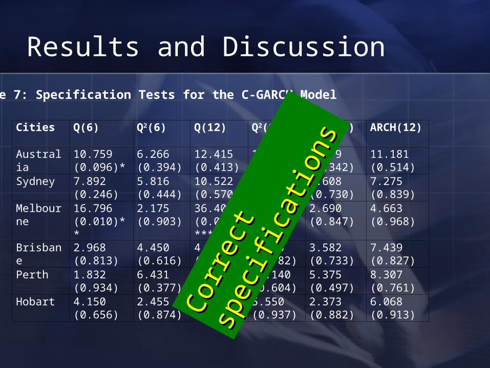
Cities Q(6) Q2(6) Q(12) Q2(12) ARCH(6) ARCH(12)

Australia 10.759(0.096)*

6.266(0.394)

12.415(0.413)

10.006(0.615)

6.779(0.342)

11.181(0.514)

Sydney 7.892(0.246)

5.816(0.444)

10.522(0.570)

7.929(0.791)

3.608(0.730)

7.275(0.839)

Melbourne 16.796(0.010)**

2.175(0.903)

36.405(0.000)***

4.340(0.976)

2.690(0.847)

4.663(0.968)

Brisbane 2.968(0.813)

4.450(0.616)

4.732(0.966)

8.035(0.782)

3.582(0.733)

7.439(0.827)

Perth 1.832(0.934)

6.431(0.377)

8.272(0.764)

10.140(0.604)

5.375(0.497)

8.307(0.761)

Hobart 4.150(0.656)

2.455(0.874)

7.585(0.817)

5.550(0.937)

2.373(0.882)

6.068(0.913)

Table 7: Specification Tests for the C-GARCH Model

Cor

rect

Cor

rect

sp

ecifi

cation

s

spec

ifica

tion

s

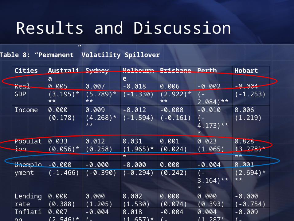
Cities Australia Sydney Melbourne Brisbane Perth HobartReal GDP 0.005

(3.195)***0.007(5.789)***

-0.018(-1.330)

0.006(2.922)***

-0.002(-2.084)**

-0.004(-1.253)

Income 0.000(0.178)

0.009(4.268)***

-0.012(-1.594)

-0.000(-0.161)

-0.010(-4.173)***

0.006(1.219)

Population 0.033(0.056)*

0.012(0.258)

0.031(1.965)**

0.001(0.024)

0.023(1.065)

0.828(3.278)***

Unemployment

-0.000(-1.466)

-0.000(-0.390)

-0.000(-0.294)

0.000(0.242)

-0.004(-3.164)***

0.001(2.694)***

Lending rate

0.000(0.388)

0.000(1.205)

0.002(1.530)

0.000(0.074)

0.000(0.393)

-0.000(-0.754)

Inflation 0.007(2.546)**

-0.004(-2.697)***

0.018(1.657)*

-0.004(-7.898)***

0.004(1.287)

-0.009(-3.756)***

Building approval

0.000(0.106)

0.000(0.424)

-0.000(-0.490)

0.001(3.472)***

0.000(0.934)

-0.000(-2.125)**

Table 8: “Permanent” Volatility Spillover

Results and Discussion

Results and Discussion

Cities Australia Sydney Melbourne Brisbane Perth Hobart

Real GDP -0.001(-0.391)

0.008(2.578)***

-0.035(-2.495)**

0.011(3.745)***

0.008(2.274)**

-0.003(-0.820)

Income 0.000(0.078)

0.010(4.240)***

-0.019(-3.333)***

0.004(3.181)***

0.016(1.484)

0.006(1.083)

Population 0.090(3.618)***

0.062(1.239)

0.050(2.460)**

0.045(2.468)**

0.040(2.986)***

-0.184(-2.542)**

Unemployment

-0.000(-0.566)

-0.000(-1.947)*

0.000(0.755)

0.000(0.678)

-0.000(-0.918)

-0.001(-2.538)***

Lending rate 0.000(1.922)*

0.001(0.811)

0.001(0.837)

0.001(2.666)***

0.001(4.018)***

0.001(2.755)***

Inflation 0.011(1.849)*

-0.009(-4.633)***

0.022(1.941)*

-0.004(-2.745)***

-0.009(-6.852)***

-0.003(-0.935)

Building approval

0.000(1.690)*

0.000(1.486)

-0.000(-0.285)

0.001(12.305)***

-0.000(-2.946)***

-0.000(-1.657)*

Table 9: “Transitory” Volatility Spillover

Conclusion

Volatility ClusteringThe volatility of housing price can be

decomposed into permanent and transitory components Differences between both components.

Both volatilities capture different sets of information and have different determinants.