256 IEEE TRANSACTIONS ON AUTOMATIC CONTROL, VOL. AC-28, NO. 3, MARCH 1983

Voyager Orbit Determination at Jupiter JAMES K. CAMPBELL, STEPHEN P. SYNNOTT, AND GERALD J. BIERMAN, SENIOR MEMBER, IEEE

Abstract--This paper summarizes the Voyager 1 and Voyager 2 orbit determination activity extending from encounter minus 60 days to the Jupiter encounter, and includes quantitative results and conclusions derived from mission experience. The major topics covered include an identifica- tion and quantification of the major orbit determination error sources and a review of salient orbit determination results from encounter, with emphasis on the Jupiter approach phase orbit determination. Special attention is paid to the use of combined spacecraft-based optical observations and Earth-based radiometric observations to achieve accurate orbit determina- tion during the Jupiter encounter approach phase.

I. INTRODUCTION

0 N March 5, 1979 after a journey of 546 days and slightly more than 1 billion km, the Voyager 1

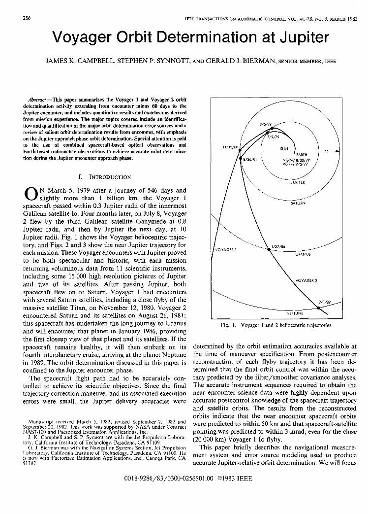
spacecraft passed within 0.3 Jupiter radii of the innermost Galilean satellite Io. Four months later, on July 8, Voyager 2 flew by the third Galilean satellite Ganymede at 0.8 Jupiter radii, and then by Jupiter the next day, at 10 Jupiter radii. Fig. 1 shows the Voyager heliocentric trajec- tory, and Figs. 2 and 3 show the near Jupiter trajectory for each mission. These Voyager encounters with Jupiter proved to be both spectacular and historic, with each mission returning voluminous data from 11 scientific instruments, including some 15 000 high resolution pictures of Jupiter and five of its satellites. After passing Jupiter, both spacecraft flew on to Saturn. Voyager 1 had encounters with several Saturn satellites, including a close flyby of the massive satellite Titan, on November 12, 1980. Voyager 2 encountered Saturn and its satellites on August 26, 1981 ; this spacecraft has undertaken the long journey to Uranus and will encounter that planet in January 1986, providing the first closeup view of that planet and its satellites. If the spacecraft remains healthy, it will then embark on its fourth interplanetary cruise, amving at the planet Neptune in 1989. The orbit determination discussed in this paper is confined to the Jupiter encounter phase.

The spacecraft flight path had to be accurately con- trolled to achieve its scientific objectives. Since the final trajectory correction maneuver and its associated execution errors were small, the Jupiter delivery accuracies were

Manuscript received March 5. 1982: re\%ed September 7. 1982 and September 20. 1982. This work was supported by NASA under Contract NAS7- 1 0 0 and Factorized Estimation Applications. Inc.

J. K. Campbell and S. P. Synnott are with the Jet Propulsion Labora- tory. California Institute of Technology. Pasadena, CA 91 109.

G. J. Bierman was Xvith the Navigation Systems Section, Jet Propulsion

is now with Factorized Estimation Applications. Inc.. Canoga Park. CA Laboraton.. California Institute of Technology. Pasadena. CA 91 109. He

9 1307.

\ VOYAGER 2

Fig. I . Voyager 1 and 2 heliocentric trajectories

determined by the orbit estimation accuracies available at the time of maneuver specification. From postencounter reconstruction of each flyby trajectory it has been de- termined that the final orbit control was within the accu- racy predicted by the filter/smoother covariance analyses. The accurate instrument sequences required to obtain the near encounter science data were highly dependent upon accurate postcontrol knowledge of the spacecraft trajectory and satellite orbits. The results from the reconstructed orbits indicate that the near encounter spacecraft orbits were predicted to withn 50 km and that spacecraft-satellite pointing was predicted to within 3 mrad, even for the close (20 000 km) Voyager 1 Io flyby.

This paper briefly describes the navigational measure- ment system and error source modeling used to produce accurate Jupiter-relative orbit determination. We will focus

00 18-9286/83/0300-0256SO 1 .OO 1983 IEEE

CAMPBELL et ul.: VOYAGER ORBIT DETERXIINATIO~U’ AT JUPITER

ID ENCOUNTER AND

\ I /

Fig. 2. Voyager I Jupiter flyby geometry.

/

Fig. 3. Voyager 2 Jupiter flyby geometry.

on the particular problem of combining the orbit informa- tion content from two distinct sources; Earth-based radio- metric observations (range and Doppler) and spacecraft- based optical observations to achieve accurate orbit de- termination during the planetary approach. Because this paper is an application of modern estimation, the reader is assumed to be familiar with the estimation concepts that are employed. The algorithmic formulations based on ma- trix factorization that are used to compute the orbit de- termination estimates, estimate error sensitivities, and estimate error covariances (filter/smoother and consider filter/smoother) are described (in great detail) in [l], [2], [6] , and [7]. The latter part of Section I1 contains a discus- sion of the merits of the SRIF/SRIS and U - D covariance factorized estimation algorithms that are used throughout this application.

The research reported here is extracted in large part from the Voyager navigation team report [8]. Interested

251

readers are urged to consult this reference and also [lo], which documents the Voyager Saturn encounter orbit de- termination.

11. NAVIGATION FILTER DESIGN RATIONALE

There were two principal reasons for using a sequential stochastic filtering algorithm to process the Voyager track- ing data. The first reason has to do with modeling of nongravitational accelerations and the second has to do with modeling of the optical data to account for pointing errors. Let us first focus on the nongravitational force problem.

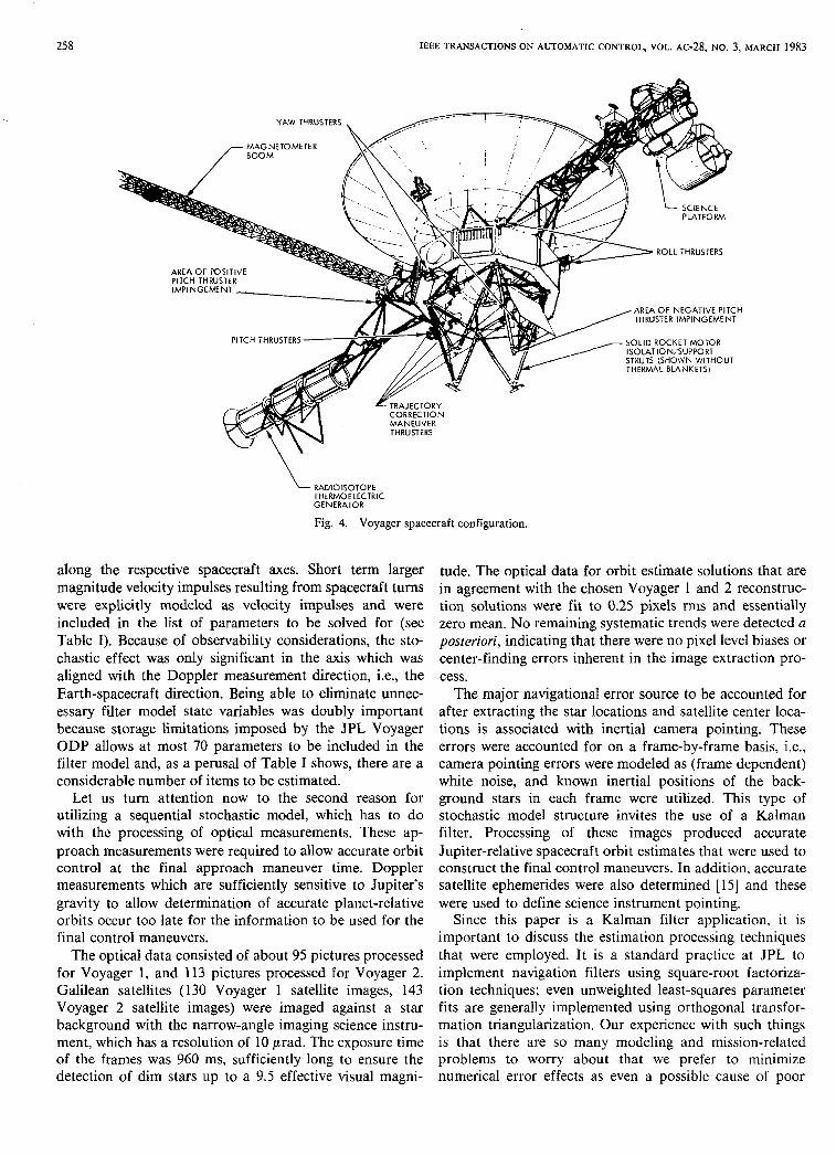
The Voyager spacecraft, shown in Fig. 4, are three-axis stabilized vehicles, and remain in an Earth-pointed orienta- tion relative to the Sun and a star, usually Canopus, for long periods of time. Notable features of the spacecraft are the large antenna dish, the science scan platform, and the groups of thrusters. The thrusters are unbalanced, since they do not fire in pairs, and are separated from the center of mass on opposite moment arms. A consequence of this configuration is that each time that a thruster is fired to either maintain or change the spacecraft attitude, there is a net translational velocity imparted to the spacecraft. Mo- tion of the scan platform puts torque on the spacecraft, requiring thruster firings to maintain alignment. The effec- tive center of solar pressure does not coincide with the spacecraft center of mass, and this can cause one-sided thruster firings.

A design flaw of the spacecraft is that the exhaust plumes from the positive and negative pitch attitude thrus- ters, which have velocity components along the radiometric measurement direction, strike the spacecraft structure. This fact was known before launch, but it was believed that the effect would be neghgible. The conclusion of a postlaunch study was that, in fact, the plume impingement effect is significant.

Spacecraft outgassing as a byproduct of attitude control was considered to be basically a dynamic stochastic process which imparted AV velocity impulses to the spacecraft. The nature of these pulses was such that over a daily period the net translational effect on the spacecraft was zero. How- ever, the Doppler tracking data were significantly cor- rupted by this attitude control pulsing. It has been known for some time [9] that estimate accuracy severely degrades when such disturbances are not accounted for in the filter model, and it was demonstrated early in the flight that the OD estimates produced from radiometric data without taking into account a dynamic stochastic process propa- gated poorly and gave inaccurate orbit predictions. Dop- pler residuals could be more accurately predicted from a previous fit which assumed a stochastic process than from a fit to the same data where stochastic effects were ignored.

These spacecraft generated forces are commonly termed spacecraft nongravitational forces. For Voyager, small atti- tude control impulses were averaged over a daily period and treated as piecewise constant stochastic accelerations

258 IEEE TRANSACTIONS ON AUTOMATIC CONTROL, VOL. AC-28, NO. 3, MARCH 1983

'.-- RADIOISOTOPE THERMOELECTRIC GENERATOR

Fig. 4. Voyager spacecraft configuration.

along the respective spacecraft axes. Short term larger magnitude velocity impulses resulting from spacecraft turns were explicitly modeled as velocity impulses and were included in the list of parameters to be solved for (see Table I). Because of observability considerations, the sto- chastic effect was only significant in the axis which was aligned with the Doppler measurement direction, i.e., the Earth-spacecraft direction. Being able to eliminate unnec- essary filter model state variables was doubly important because storage limitations imposed by the JPL Voyager ODP allows at most 70 parameters to be included in the filter model and, as a perusal of Table I shows, there are a considerable number of items to be estimated.

Let us turn attention now to the second reason for utilizing a sequential stochastic model, which has to do with the processing of optical measurements. These ap- proach measurements were required to allow accurate orbit control at the final approach maneuver time. Doppler measurements which are sufficiently sensitive to Jupiter's gravity to allow determination of accurate planet-relative orbits occur too late for the information to be used for the final control maneuvers.

The optical data consisted of about 95 pictures processed for Voyager 1, and 113 pictures processed for Voyager 2. Galilean satellites (130 Voyager 1 satellite images, 143 Voyager 2 satellite images) were imaged against a star background with the narrow-angle imaging science instru- ment, which has a resolution of 10 prad. The exposure time of the frames was 960 ms, sufficiently long to ensure the detection of dim stars up to a 9.5 effective visual magni-

tude. The optical data for orbit estimate solutions that are in agreement with the chosen Voyager 1 and 2 reconstruc- tion solutions were fit to 0.25 pixels rms and essentially zero mean. No remaining systematic trends were detected a posteriori, indicating that there were no pixel level biases or center-finding errors inherent in the image extraction pro- cess.

The major navigational error source to be accounted for after extracting the star locations and satellite center loca- tions is associated with inertial camera pointing. These errors were accounted for on a frame-by-frame basis, i.e., camera pointing errors were modeled as (frame dependent) white noise, and known inertial positions of the back- ground stars in each frame were utilized. This type of stochastic model structure invites the use of a Kalman filter. Processing of these images produced accurate Jupiter-relative spacecraft orbit estimates that were used to construct the final control maneuvers. In addition, accurate satellite ephemerides were also determined [15] and these were used to define science instrument pointing.

Since this paper is a Kalman filter application. it is important to discuss the estimation processing techniques that were employed. It is a standard practice at JPL to implement navigation filters using square-root factoriza- tion techniques; even unweighted least-squares parameter fits are generally implemented using orthogonal transfor- mation triangularization. Our experience with such things is that there are so many modeling and mission-related problems to worry about that we prefer to minimize numerical error effects as even a possible cause of poor

CAMPBELL ef Ol . : VOYAGER ORBIT DETERMINATION AT JUPITER 259

TABLE I 67 STATE VOYAGER NAVIGATION MODEL WITH ESTIhiATION

RESULTS BASED ON ENCOUNTER DATA FROM FEBRUARY9-MARCH 18,1979

s ta te A Posteriori

A priori Sigm (smoothed siscas) R W k B

Cartesian positions (3) 500.0 Ian Cartesian ve loc i t i e s (31 .5 d s

Line-of-sight (s/c - EaFth) mn-gravitational accelerations

b i a s (1) 5 . G ~ 1 0 - ~ ~ kds2 piecewise constant random (1) 5 . 0 ~ 1 0 - ~ ~ W s 2

50.0 d / s 2

600.0 d / s 2

camera pointing angles (3)

clock, cone 0.3 deg

Mst 1.0 dep

88.0 Ian 0.06 d s

2.5x10-12 W s 2 1 . 5 ~ 1 0 - l ~ W s 2

o . a & W s 1.GX10y w s

50.0 lua

5.0 &/s2

40.0 &/s2

200.0 !an

0.4 m 0.5 m 1.0 lua

1 . O x l O ~

0.2 deE

Smwthed values are FXS

m. over the 108-step time

Smmthed value is F34S over the l o b s t e p time arc.

only 6 cross-track (mobsemable) .:V ccmpollents included.

RHs of the 19 pararmeters.

3 tracking stat ions.

Range measureaent biases, one for each stat ion.

Prame (white) Independent from frame to

aver 87 fremes. h t h e d values AHS

A priori Smoothed Estimate Uncertainty residuals B Data Points

Radimtric:

Doppler (60 seo. sample average) 1.0 d s 0.4 mm/s 2400

Range 1.0 Ian 0.1 lua n optical 0.5 pixels 0.25 pixels 139 stars

101 satellite iuages

filter performance. Our concerns are illustrated in [ 113 which summarizes some of the peculiar (and wrong) numerical results that were obtained in premission simula- tions of the Voyager Jupiter approach using conventional Kalman filter covariance formulations.

The Earth-based radiometric data are processed using a batch sequential, square-root information filter/smoother [l], [ 2 ] , and ["I, and the spacecraft-based optical data are processed with a U - D covariance factorized Kalman filter [2], [6]. The radiometric observation set is much larger than the set of optical observations; for the encounter applica- tion reported here the radiometric data consisted of 2400 Doppler and 27 range measurements and the optical data set consisted of 139 stars and 101 satellite images. The data types and associated statistics are summarized in Table 11. As is pointed out in [2] the SRIF is computationally more

efficient for larger data sets than is the Kalman filter. It is of interest to note that, despite this, when the other ancillary aspects of the problem are included (such as integration of the variational equations and computation of the measure- ment observables and differential correction estimate par- tial derivatives), the difference in computational cost (as will be shown in the following paragraphs) turns out to be relatively unimportant.

To give an idea of the computational burden that is involved, consider a typical radiometric SRIF/SRIS solu- tion with 67 state variables (Table I). This model contains only 4 process noise states (line-of-sight acceleration and 3 camera pointing errors); there are 3500 data points and 132 time propagation steps. The problem run on a UNI- VAC 1110, in double precision, used 275 CPU s for filtering; smoothed solutions and covariance computation

260 IEEE TR4NSACTIONS ON AUTObMTIC CONTROL, VOL. AC-28. NO. 3, MARCH 1983

used 265 CPU s. The entire run scenario including trajec- tory variational equation integration, observable partials generation, solution mapping, and generation of smoothed residuals used 4320 CPU s. Thus, the filter and smoother portion each involved little more than 6 percent of the CPU time. Two points of note, in regard to these sample run times are as follows.

1) We generally iterate and generate several filter/smoother solution sets for a given nominal trajectory and file of observation partials. Smoothed covariances use the lion’s share of the smoother computation and these need only be computed for the last iteration.

2) The program inputs were not configured to minimize filter/smoother CPU requirements.

For this dynamic state configuration optimally arranged smooth code should require less than 25 percent of the CPU time required for the filter phase. The point we are aiming at is that, based on our experience in [l l] , a conventional Kalman filter covariance formulation would execute in essentially the same amount of CPU time (& 15 percent), and evidently the filter CPU cost is small com- pared with total run CPU time requirements.

As pointed out in [l] the pseudoepoch state formulation model is an evolutionary outgrowth of the least-squares initial condition estimator [3]. If X,? represents current time position and velocity differential correction estimates, then the pseudoepoch state x/” is defined by the equation

x , ’ = @ . ~ ~ ( t J ~ t o ) x J + @ ~ X y ( c J ’ t ~ ) ~ + ~ ~ X p ( t J ’ t J ~ ~ ) P ~ ~ ~

where the components of y are bias parameters and the components of vector pJ - , are piecewise constant stochas- tic model parameters. The transition matrices @.xx( t J , to).

( t , : to 1 and

@ x X p ~ ~ j ~ ~ , - l ~ = @ ~ ’ ~ ~ , ~ ~ o ~ @ . ~ ~ ~ ~ ~ ~ ~ o ~

- ~ ~ ‘ ( f j - l , f o ) @ ~ ~ ( ~ j - , , t o )

are obtained by integrating variational differential equa- tions for

[ @ x . x ( t 7 t o > 9 @ x , , ( L to) ,@& t o ) ]

from an epoch time to. In Table I the filter state vector x , y , and p components are defined.

Orbit determination problems with radiometric data are ill-conditioned. This is due, in the main, to poor observabil- ity. and large dynamic ranges of the variables that are involved (viz. acceleration errors - 10 - I 2 km/s’, range values - lo8 km, etc). The observability problem is aggra- vated by the inclusion of large numbers of parameters (such as ephemerides) that are very weakly coupled to the spacecraft observables. The two features of the SRIF/SRIS algorithmic formulation that are most important for this application are as follows.

1) Numerical reliability: The SRIF/SRIS algorithms are the most (numerically) accurate and reliable formulation of the Kalman filter/smoother known. Because of the com- plexity and difficulty inherent in the formulation of the

deep space navigation problem it is most important that the estimates and covariances be computed correctly.

2 ) Computational efficiency: The algorithms are for- mulated so as to exploit the structure of the orbit de- termination problem. In particular. there are many mea- surements to be processed per time propagation step, the dynamical model involves only a small number of stochas- tic variables, there are a preponderance of bias parameters, and the position-velocity states are cast in a pseudoepoch state formulation. Early tests demonstrated that the SFUF, for this structure, was more efficient than a conventional (and less reliable) Kalman filter mechanization.

Using the SRIF it is relatively easy to take the processed results and generate estimates that correspond to models with a smaller number of bias parameters. This feature is especially useful for confirming that parameters thought to be of little significance turn out, in fact, to have little effect on the key estimate state vector components.

The U - D covariance factorization was chosen to mecha- nize the optical navigation filter for many of the same reasons (numerical reliability and computational effi- ciency), except in this case the measurement set per time propagation is small, and for such problems the U - D formulation is more efficient than the SRIF. In [ l l ] the U- D formulation and the Kalman filter both conventional (optimal) and stabilized (Joseph/suboptimal) forms are compared for a Jupiter approach simulation with radiomet- ric data. In the tests reported there the covariance mecha- nized filters performed very poorly; they gave results that ranged from inaccurate, but whch might be thought cor- rect (20-50 percent errors) to impossible (negative vari- ances and estimates that were absurd). It happens that optical navigation data are not nearly as ill-conditioned as are the radiometric data, and in fact, the early optical navigation studies successfully carried out in [5] used a conventional Kalman filter mechanization. The decision to use a U - D factorization in place of the conventional mechanization was based on the following facts:

1) Comparisons (operation counts, actual CPU, and storage requirements) show that optimally coded U- D and conventional covariance mechanizations are nearly indis- tinguishable in terms of storage and computational require- ments.

2) U- D factor mechanization has accuracy that is com- parable with the SRIF. On the other hand, one cannot be certain when the covariance mechanization will degrade or fail (e.g., when the a priori uncertainties are too large. the measurement uncertainties are too small, the data geome- try is near linearly dependent, etc., one can expect stability and accuracy problems).

It is the conviction of (one of) the authors (who is believed by the others!) that covariance mechanized Kalman filters should newer be computer implemented. Further, it is believed that if the Kalman filter applications community had more experience with efficiently and relia- bly mechanized factorization alternatives, there would be few instances where a covariance mechanized Kalman filter would find application. We note in closing this factoriza-

CAMPBELL et (I/.: VOYAGER ORBIT DETERhiINATION AT JUPITER 26 1

TABLE111 SUMMARY OF JUPITER APPROACH ORBIT CONTROL

Voyager 1 TCM Execut ion Time CB. R 8 - T LT Designed Achieved

A l l , mlsec 5 8 , KJr

3 E - 35 days 4.146 4.208 -1725. +!3125. toh 14m

4 E - 12.5 days 0.586 0.594 +7iO. -100. - O h Om 14’

Voyaqer 2 TCM

3 E - 45 days 1.442 1.386 +3330. t5040. -Oh 4m 42’

4 E - 12 days 0.576 0.574 -895. +? lo . +Oh Om 03’

tion algorithm discussion that the SRIF and U - D algo- rithms that were used in this application have been refined and generalized, and are commercially available in the form of portable Fortran subroutines [12].

111. OD PERFORMANCE

This section will summarize the near-encounter OD re- sults for both spacecraft. These results are 1) the orbit determination that was done to deliver the Voyager spacecraft to their required final target points met the required accuracies; and 2) that the final postdelivery orbit determination needed to accurately point science instru- ments in the near and postencounter phases also exceeded specification accuracies. A limitation of the Voyager orbit determination program is that one can include at most 70 filter states, and this includes the sum of both estimated and consider filter states. For completeness we remind the reader that consider parameters, cf. [ 11 and [2], play no role in the estimation except to provide a deweighting to the confidence one would otherwise put on the estimates. As noted earlier, the size limitation does not allow us to include all the known error sources in the filter model. Table I lists one of the several filter models that were used, and quantifies the results obtained. Observe that although there are 12 maneuvers only six cross-track maneuver correction terms are included, and these terms have a neghgible effect on estimator performance. This conclusion is based both on estimate comparisons with and without such terms included and on the incremental change in the computed covariance due to the addition of consider parameter sensitivity effects. The discussion that follows is an elaboration of the results summarized in Table I.

Jupiter Approach Solutions

For approximately the last 60 days of each approach, both radio and optical data were continuously acquired to allow orbit estimates to be revised every few days. Optical data in the time period beginning 60 days from encounter ( E ) to E - 30 days were acquired at the rate of approxi- mately one picture per day, and this rate increased to about four or five pictures per day in the last few days before encounter. Radio tracking (coherent Doppler and

range) was virtually continuous for the last 60 days of approach. For each encounter, there were several critical events for which orbit estimate deliveries to certain ele- ments of the project were required. The events consisted of two trajectory correction maneuvers, at about E -40 days and E - 12 days, and several updates to the onboard instrument pointing, a critical element in the near encoun- ter science return. The detailed summary of the delivery events for each spacecraft is shown in Table 111.

Based on a preliminary data acquisition schedule, covari- ance analysis estimates were computed preflight of the orbit determination errors which would result at these various delivery times. The primary purpose of this section is to compare the near real-time filter and the current best reconstructed smoothed orbit estimates, and also to com- pare both of these to the expected covariance performance computed preflight. It will be shown that all orbit estimates but one fell well within the expected preflight capability (1 - u) even though those early statistics were derived with unrealistic, very optimistic, assumptions about the “small” nongravitational forces caused by spacecraft attitude changes.

More specifically, as discussed in Section 11, the spacecraft’s attitude control system did not employ cou- pled thrusters, and hence there were many small velocity impulses imparted to the spacecraft. These velocity im- pulses are impossible to model individually, and affect (to a sensible level) the meter level ranging and submillime- ter/second Doppler observables if they are imparted along the Earth-line. In addition, whenever the spacecraft orien- tation was changed to allow an engineering calibration, or a science scan of the Jovian system, velocity impulses of tens of millimeters per second were imparted. These larger impulses were not accounted for in the preflight analysis, and the more continuous smaller impulses resulted effec- tively in accelerations of the order of 5- 10 x 10 - l 2 km/s2 along all three spacecraft axes. The larger impulsive veloc- ity changes have two effects. When they occur within the data arc, an estimate of their components becomes con- fused with the estimates of the dynamically important parameters, and the result is an incorrect orbit; when they occur past the end of the data arc they cause incorrect mapping to the encounter time, and the result is an incor- rect prediction of encounter conditions. Based on covari-

262 IEEE TRANSACTIONS ON AUTOMATIC CONTROL, VOL. AC-28, NO. 3, MARCH 1983

ance analyses, it did not appear possible to accurately predict the velocity components at the maneuver event times from a priori information.

Data Weighting

In the vicinity of a planetary encounter, the radio and optical data are geometrically complementary. The Earth- spacecraft line-of-sight range and velocity measurements indirectly provide the spacecraft-planet distance through observable dynamic effects, and the optical data effectively measure the instantaneous spacecraft-satellite cross line- of-sight position relative to a particular satellite. The radio and optical data were planned to allow determination of both the satellite orbits and the spacecraft trajectory rela- tive to the planet.

In the estimation process using both radio and optical observations, the solutions at certain stages were found to be sensitive to the relative weighting of the two data types. Based on the image extraction analysis, the optical data were thought to measure the star and satellite center loca- tions to 0.5 pixels or less in a random measurement noise sense. In addition, if there were any systematic optical image extraction errors, they were thought to be small ( < 0.5 pixels) and to behave as biases in the 2-D picture space, or as long term slowly varying functions, i.e., nearly biases. Using these arguments the optical data usually were assumed to have 0.5 pixel measurement noise; 0.5 pixel optical biases were used as consider parameters to compute the expected uncertainty in the orbit estimates. Inciden- tally, these two consider parameters, together with the 67 estimated parameters listed in Table I, essentially exhausts the 70 parameter ODP storage limitation.

After calibrating for troposphere, ionosphere, and space plasma effects, the measurement errors for radio data are equivalent to only a few meters in range and 0.3-0.5 mm/s for a 60 s count time for Doppler. However, because of the known level of unmodelable nongravitational accelerations, range was more usually weighted at 100 m, and Doppler at 1 m / s , for a 60 s count time. These values, together with the postfit rms residual results are displayed in Table 11. For the radio data, the most likely sources of error are transmission media calibration errors and Earth station location errors, both of which are usually combined into an assumed systematic error uith a diurnal signature. Data noise for Voyager 2 was larger because its view periods occurred during local daylight hours, when transmission media effects were larger. The Voyager 2 encounter also coincides with a more active solar period.

Reconstruction of Encounter Orbits

Since the encounters, it has been possible to do a de- tailed analysis of the larger nongravitational impulsive events for Voyager 1, using data from approximately 60 days after encounter. In addition to errors associated with the two-approach TCMs, there occurred 10 preencounter events whose effects were hrectly observable along the Earth-line and whch therefore were estimated as impulsive

VOYAGER I RECONSTRUCTED APPROACH SOLUTIONS RELATLVE TO FINAL RECONSTRUCTED TRAJECTORY

Y \ \

01 I I I I I -30 -25 -20 -15 -1 0 -5

DAYS FROM ENCOUNTER

Fig. 5 . Reconstructed history of Voyager 1 B . R solutions relative to postencounter reconstructed orbit.

AVs; these are the 12AV state vector components included in Table I.

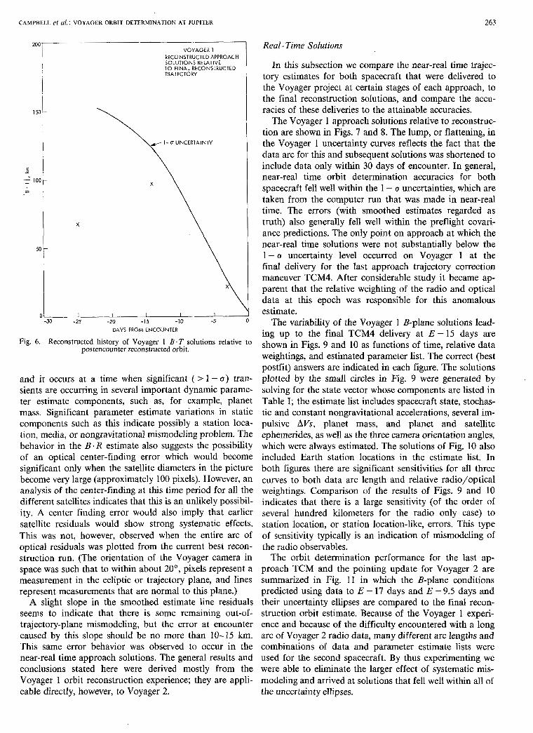
One of the best ways to measure the real limit to the orbit determination capability as a function of time to encounter is to examine the variation in solutions along a trajectory which has already passed through several estima- tion iterations for the magnitude of the impulsive compo- nents. With as detailed a treatment of the larger impulsive events as is possible, and with stochastic and constant acceleration components solved for in the sequential filter to remove any excess nongravitational effects, the relative time history B-plane’ solutions for the last 25 days before Voyager 1 encounter were computed and are displayed in Figs. 5 and 6 along with the 1 - (I uncertainties in these solutions. These uncertainties were calculated using no assumed systematic errors in either radio or optical data, such as optical biases, and therefore represent lower limits to the error that could be expected. In general, the solu- tions fall within even this optimistic uncertainty level. The 55 km A B . R solution at E - 3.5 days is the only anomaly

plane passing through the center of a target planet and perpendcular to ‘Planetary targeting is usually expressed in terms of the E-plane, a

the incoming approach hyperbola asymptote of a spacecraft. ‘‘B‘T” is the intersection of the B-plane with the ecliptic and ‘ ‘B .R” is a vector in the B-plane that is perpendicular to B . T and making a right-handed system R, S. T, where S is the incoming asymptote.

CAMPBELL ef o/.: VOYAGER ORBIT DETER\fINATION AT JUPITER 263

2w VOYAGER 1

RECONSTRUCTED APPROACH SOLUTIONS RELATIVE TO FINAL RECONSTRUCTED TRAJECTORY

01 I I I I I -30 -25 -20 -15 -10 -5

DAYS FROM ENCOUNTER

Fig. 6. Reconstructed history of Voyager I B .T solutions relative to postencounter reconstructed orbit.

and it occurs at a time when significant ( > 1 - o) tran- sients are occumng in several important dynamic parame- ter estimate components, such as, for example, planet mass. Significant parameter estimate variations in static components such as this indicate possibly a station loca- tion, media, or nongravitational mismodeling problem. The behavior in the B. R estimate also suggests the possibility of an optical center-finding error which would become significant only when the satellite diameters in the picture become very large (approximately 100 pixels). However, an analysis of the center-finding at this time period for all the different satellites indicates that this is an unlikely possibil- ity. A center finding error would also imply that earlier satellite residuals would show strong systematic effects. This was not, however, observed when the entire arc of optical residuals was plotted from the current best recon- struction run. (The orientation of the Voyager camera in space was such that to within about 20°, pixels represent a measurement in the ecliptic or trajectory plane, and lines represent measurements that are normal to this plane.)

A slight slope in the smoothed estimate line residuals seems to indicate that there is some remaining out-of- trajectory-plane mismodeling, but the error at encounter caused by this slope should be no more than 10-15 km. T h s same error behavior was observed to occur in the near-real time approach solutions. The general results and conclusions stated here were derived mostly from the Voyager 1 orbit reconstruction experience; they are appli- cable directly, however, to Voyager 2.

Real - Time Solutions

In this subsection we compare the near-real time trajec- tory estimates for both spacecraft that were delivered to the Voyager project at certain stages of each approach, to the final reconstruction solutions, and compare the accu- racies of these deliveries to the attainable accuracies.

The Voyager 1 approach solutions relative to reconstruc- tion are shown in Figs. 7 and 8. The lump, or flattening, in the Voyager 1 uncertainty curves reflects the fact that the data arc for this and subsequent solutions was shortened to include data only within 30 days of encounter. In general, near-real time orbit determination accuracies for both spacecraft fell well within the 1 - u uncertainties, which are taken from the computer run that was made in near-real time. The errors (with smoothed estimates regarded as truth) also generally fell well within the preflight covari- ance predictions. The only point on approach at which the near-real time solutions were not substantially below the 1 - a uncertainty level occurred on Voyager 1 at the final delivery for the last approach trajectory correction maneuver TCM4. After considerable study it became ap- parent that the relative weighting of the radio and optical data at this epoch was responsible for this anomalous estimate.

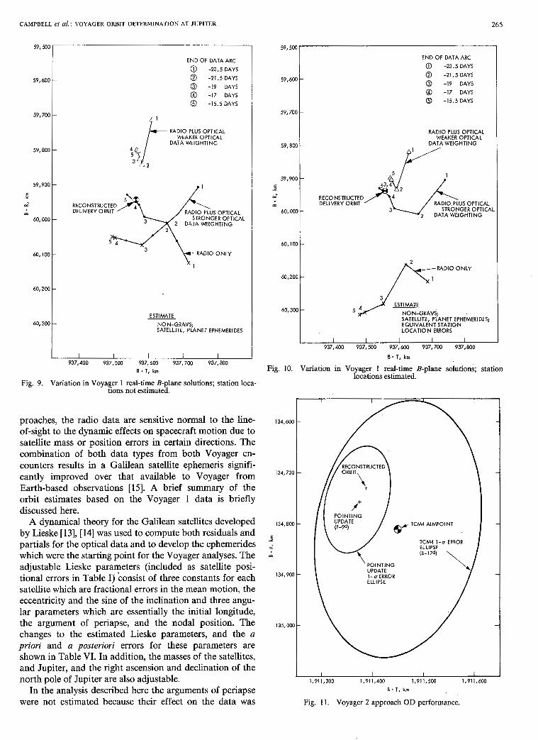
The variability of the Voyager 1 B-plane solutions lead- ing up to the final TCM4 delivery at E - 15 days are shown in Figs. 9 and 10 as functions of time, relative data weightings, and estimated parameter list. The correct (best postfit) answers are indicated in each figure. The solutions plotted by the small circles in Fig. 9 were generated by solving for the state vector whose components are listed in Table I; the estimate list includes spacecraft state, stochas- tic and constant nongravitational accelerations, several im- pulsive AVs, planet mass, and planet and satellite ephemerides, as well as the three camera orientation angles, which were always estimated. The solutions of Fig. 10 also included Earth station locations in the estimate list. In both figures there are significant sensitivities for all three curves to both data arc length and relative radio/optical weightings. Comparison of the results of Figs. 9 and 10 indicates that there is a large sensitivity (of the order of several hundred kilometers for the radio only case) to station location, or station location-like, errors. This type of sensitivity typically is an indication of mismodeling of the radio observables.

The orbit determination performance for the last ap- proach TCM and the pointing update for Voyager 2 are summarized in Fig. 11 in which the B-plane conditions predicted using data to E - 17 days and E - 9.5 days and their uncertainty ellipses are compared to the final recon- struction orbit estimate. Because of the Voyager 1 experi- ence and because of the difficulty encountered with a long arc of Voyager 2 radio data, many different arc lengths and combinations of data and parameter estimate lists were used for the second spacecraft. By thus experimenting we were able to eliminate the larger effect of systematic mis- modeling and arrived at solutions that fell well within all of the uncertainty ellipses.

264 IEEE TRANSACTIONS ON AUTOMATIC CONTROL, VOL. AC-28, NO. 3 , MARCH 1983

VOYAGER 1 APPROACH SOLUTIONS RELATIVE TO F I N A L RECONSTRUCTED TRAJECTORY

. \ \

1 -

*

\ 1 -

I -

I -

I -

l -

) I I I I I I 1 X I -45 -40 -35 -30 -25 -20 -15 -10 -5

DAYS FROM ENCOUNTER

\ \

PREFLIGHT I - U ‘ U N C E R T A I N W /

X

APPROACH SOLUTIONS RELATIVE TO F I N A L RECONSTRUCTED TRAJECTORY

\\ \

X \ \

I - U U N C E R T A I N W

\ \

PREFLIGHT I - U ‘ U N C E R T A I N W

X

Fig. 7. History of Voyager 1 real-time B . R solutions relative to posten- counter reconstructed orbit.

\

@An F W M EKWNIE1

Fig. 8. History of Voyager I real-time B . T solutions relative to posten- counter reconstructed orbit.

Tables IV and V indicate the OD delivery performance for each spacecraft. The last columns of each table show that the delivery OD performance for each spacecraft easily met the established accuracy criteria. In the case of Voyager 2, the delivery requirements were less stringent, and the achieved delivery was nearly equivalent to 0.5

tion of the overall capability and performance of the Voyager radiometric data. Fig. 12 shows, in geocentric angular coordinates, the shift in Jupiter position coordi- nates obtained from a set of orbit estimates based on radiometric data arcs extending from E - 60 to E + 30 days. This data arc allows for an accurate Jupiter-relative orbit estimate and some sensitivity to Jupiter ephemeris error. One solution estimates only ephemeris error; the second solution estimates both ephemeris and station loca- tion errors, and essentially trades off these two error sources to give the same net geocentric angular offset as the ephemeris-only solution. This plot indicates the general inability of Earth-based radiometric data to fully dis- tinguish station location error from ephemeris error, and sets a lower bound of about 0.25 prad to the Voyager radiometric performance. Fig. 13 plots in geocentric angu- lar coorchnates the radio-based OD that was done for the final Voyager 1 delivery, and compares this real-time result with the best reconstructed orbit at the delivery point, obtained using a combined radio plus optical data set. This plot shows that the radiometric OD for Voyager 1 per- formed to about the 0.5 prad level.

V. SATELLITE STATE ESTIMATES

A natural fallout of using the optical and radio data in the spacecraft trajectory determination process is the im- provement in the knowledge of the orbits of the four Galilean satellites. The optical data are directly sensitive to

pixel, Jupiter relative. Figs. 12 and 13 give a brief indica- satellite position changes. Near the satellite close ap-

CAMPBELL el a/.: VOYAGER ORBIT DETERhl INATlON AT JUPITER

59,jOo

END OF DATA ARC @ -23.5 DAYS

@ -21.5 DAYS @ -19 DAYS @ -17 DAYS @ -15.5 DAYS

/ 1

RADIO PLUS OPTICAL

DATA WEIGHTING WEAKER OPTICAL

‘ s J 2 3 c, . 1

2 DATA WEIGHTING STRONGER OPTICAL

RADIO ONLY

ESTIMATE NON-GRAVS; SATELLITE, PLANET EPHEMERIDES

I I I I I 937,400 937,500 537,600 937.700 937.800

6 - T , h

Fig, 9. Variation in Voyager 1 real-time B-plane solutions; station loca- tions not estimated.

proaches, the radio data are sensitive normal to the line- of-sight to the dynamic effects on spacecraft motion due to satellite mass or position errors in certain directions. The combination of both data types from both Voyager en- counters results in a Galilean satellite ephemeris sigmfi- cantly improved over that available to Voyager from Earth-based observations [15]. A brief summary of the orbit estimates based on the Voyager 1 data is briefly discussed here.

A dynamical theory for the Galilean satellites developed by Lieske [ 131, [ 141 was used to compute both residuals and partials for the optical data and to develop the ephemerides which were the starting point for the Voyager analyses. The adjustable Lieske parameters (included as satellite posi- tional errors in Table I) ‘consist of three constants for each satellite which are fractional errors in the mean motion, the eccentricity and the sine of the inclination and three angu- lar parameters which are essentially the initial longitude, the argument of periapse, and the nodal position. The changes to the estimated Lieske parameters, and the a priori and a posteriori errors for these parameters are shown in Table VI. In addition, the masses of the satellites, and Jupiter, and the right ascension and declination of the north pole of Jupiter are also adjustable.

In the analysis described here the arguments of periapse were not estimated because their effect on the data was

265

END OF DATA ARC

@ -23.5 DAYS @ -21.5 DAYS

@ -19 DAYS @) -17 DAYS 0 -15.5 DAYS

RADIO PLUS OPTICAL

DATA WEIGHTING WEAKER OPTICAL

5 4 J x G R A m ; ESTIMATE SATELLITE, PLANET EPHEMERIDES; EQUIVALENT STATION LOCATION ERRORS

I I I I I 937,400 937,Mo 937,600 937,700 937,800

6 . T, km

Fig. IO. Variation in Voyager 1 real-time B-plane solutions; station locations estimated.

1,911,300 1,911,400 1,911,500 1,911,600 B . T , km

Fig. 11. Voyager 2 approach OD performance.

266 IEEE TRANSACTIONS ON AUTOhlATIC CONTROL, VOL. AC-28, NO. 3, MARCH 1983

TABLE IV SUXMARY OF VOYAGER 1 NAMGATION DELIVERY PERFOFNANCE

Contro l Parameter Rat ionale Target Value Achieved A l lowable Actual V a l u e E r r o r E r r o r

e n t r y Geocen t r i c occu la t i on T im ing o f Jup i te r March 5 , 1979 March 5 , 1979 30 +] .4

o c c u l a t i o n l i m b s c a n a t 15:35:20.7 15:45:22.1

D is tance o f f cen ter - l ine Guarantee sampl ing -7 .4 km o f f l u x t u b e

+lo1 km 1000 km 108 km

model, km f l u x t u b e

Io c loses t app roach t i m e

Io mosa ick ing sequence control 15:13:18.9

Rarch 5 , 1979 Parch 5 , 1979 20 sec +1.8 sec 15:13:20.7

o f c u r r e n t i n Io

F ina l de l i ve ry maneuver was e x e c u t e d 1 2 . 5 d a y s p r i o r t o J u p i t e r c l o s e s t a p p r o a c h .

TABLE V SU~~MARY OF VOYAGER 2 NAVIGATION DELIVERY PERFORMANCE

Contro l Parameter Rat ionale Target Value Acbieved Expected 1-0 Actual !r,l ue Performance Error

J u p i t e r B - p l a n e coo rd ina tes

Min imize magn i tude B.R = 134,806 km 134,730 km of p o s t - J u p i t e r B . T = 1,911,454 km 1,311,337 km

223 km -74 km

TCM5 161 km -67 km

J u p i t e r c l o s e s t P o i n t i n g c o n t r o l approach t ime

7 9 79 o f E a r t h l i n e TCM5 2Zh2$& GMT 2 2 $19679 29 1.6 s GMT 22 sec +1.6 s e t

F ina l de l i ve ry maneuver was executed 12 d a y s p r i o r t o J u p i t e r c l o s e s t a p p r o a c h .

~~~ ~

“I I I I I

! - -- ESTIMATE EPHEMERIS FOR EPHEMERIS AND NOMINAL REFERENCE l,

i ONLY STATION LOCATIONS ,’/ ~ - ESTIMTE EPHEMERIS a

STATION LOCATIONS 0.1 -

v 0.2 - e L

2 2 2 0.3- -I

Q

u i? 0 .4-

U

0

$ P

0.5 -

0.6 -

LOCATKIN UNCERTAINTY

. - . . . . - , .

STATION

SOLUTION AA = 0.3m Ars = 0.3m

0.7 I I I I -0.5 -0.4 -0.3 -0.2 -0.1

GEOCENTRIC ART ASCENSION, grad

Fig. 12. Indication of Voyager 1 r a d i o m e t r i c capability.

know to be small (less than about 15 km). Mean motions, whose values were extremely well-detemined from many years of Earth-based data were also not included.

A comparison of the formal standard errors in Cartesian coordinates determined from the Earth-based and Voyager 1 data (using the Earth-based estimates as a priori) is

or---

0.5 -

0 e a 0.4 - 0 i 2 - 2

0.3 - 4 2

; 0.2 !2

c z

-

0

REAL TIME RADIO-ONLY DELIVERY ORBIT MAPPED TO ENCOUNTER

GEOCENTRIC ART ASCENSION, grad

Fig. 13. V o y a g e r 1 r a d i o m e t r i c p e r f o r m a n c e at delivery

shown in Table VI1 in which the entries represent the RSS of the sigmas and the changes in the three components of position of each satellite at the epoch of Voyager 1 Jupiter closest approach. The Voyager 1 a posteriori errors are very similar for all the satellites with the slight differences explainable by the variability of optical data distribution and quantity, and by the ratio of the satellite periods which affects the “average quality” of the data around the ob- served orbits. The Cartesian changes at the encounter

CAMPBELL et d : VOYAGER ORBIT DETERMINATION AT JUPITER 267

TABLE VI CHANGES TO ESTIMATED LIESKE PARA?%lE.TERS

Lieske Parameter A a p o s t e r i o r i E a r t h - b a s e d 0 a p r i o r i

G

e c c e n t r i c i t y

s i n e i

l o n g

node

po l e

S a t e l l i t e , J u p i t e r masses

SEPS 16

SEPS 18 5EPS 17

SEPS 19

SEPS 21 SEPS 22 5EPS 23 SEPS 24

5BET 01 5BET 02 SBET 04

5BET 11 5BET 12 5BET 13 SBET 14

!?A ZACPL 5 DEC ZOEPL 5

503 GU 501 l.24

504 GM m 5

- .175

- .013 - ,0022

.0024

-. 134 - .0082

-.0114 ,0032

- .0014 - .0045 - .0054

7.5 .512 ,407

- .551

- .0003 ,0064

29.4 3.6 7.5

657.5

.213

.179

.0071

.0013

.174

.0066

.020

.018

.0028 ,0011 ,0005

5.7

1.16 .575

,817

.0084

.0049

4.6 3.5 1.4

24.7

.42

.26

.019

.0036

.41

.025

.050

.ll

.017

.004

.005

18.0 1.05 2.5 2.4

.05

.026

56 76

1200 47

TABLE VI1 COMPARISON OF CARTESIAN FORMAL STANDARD ERRORS AND

CORRECTIONS

a p r i o r i a p o s t e r i o r i ziz:; E a r t h Based Voyager

G G

Io 87 20 35

Europa 137 28 43

Ganymede 161 34 BO

C a l l i s t o 448 35 180

Computed from Voyager 1 Encounter Data. Numbers shown a r e RSS of x , y , z components. Epoch o f C o r r e c t i o n s = March 5, 1979 12:05 GYT

epoch are well within the Earth-based a priori, but may vary somewhat at other points of the orbit. Only changes to the longitudes of Europa and Callisto were of the order of an a priori sigma. It is apparent that the a priori ephemeris was an excellent product.

VI. CONCLUSIONS

We have shown that the orbit determination performed to deliver each spacecraft to its target at Jupiter was within the predicted capability of the radiometric and optical-based navigation system for Voyager, and in fact improved for Voyager 2 as a result of the Voyager 1 experience. The postdelivery OD knowledge solutions done to refine scan platform pointing were well within the stated requirement, even though the knowledge epochs were earlier than anticipated prelaunch.

Numerous tests were made throughout the mission to test estimate consistency and accuracy of the SRIF/SRIS and U-D algorithm implementations. The navigation estimation software performed flawlessly. Indeed, the

estimation software performed so well that most of the time it was taken for granted by the navigation team, and that is the ultimate compliment.

As a result of having actually used satellite images to perform Jupiter and satellite-relative navigation, it has been determined that several prelaunch hypotheses regard- ing error sources for optical measurements were not cor- rect. Specifically, before the encounter experience it was assumed that center-finding errors for large satellite images would scale with the size of the image. From a detailed analysis of hundreds of images it was found that the center finding errors were more likely to either decrease with increasing image size, or to remain essentially constant. As indicated in Table I1 the rms noise associated with the optical measurement postfit residuals were found to be about 0.25 pixel as compared with the 1.0 pixel error assumed prelaunch. It is to be expected that the postfit residuals should have a smaller rms than the data noise (I because it is known that the postfit residual z, - Hxj , has VarianCe

- HP/,,H?

In addition, we have learned that the combination of radiometric with optical measurements must be done care- fully, with regard to the information content of each data type. This was especially true in the case of Voyager, which represented a distinct extreme in the level of dynamical corruption of the radiometric signal by small spacecraft- generated velocity pulses, that did not affect the corre- sponding optical data.

ACKNOWLEDGMENT

J. E. Reidel provided much of the postencounter com- puter support for this paper.

268 3E TRANSACTIONS ON AUTOMATIC CONTROL., VOL. AC-28, NO. 3, hiARCH 1983

REFERENCES

G. J. Bierman. “Sequential least-squares using orthogonal transfor- mations.” Jet Propulsion Lab., Pasadena. CA, Aug. I . 1975. Tech. Memorandum 33-735. G. J. Bierman, Factorization Methods For Discrete Sequential E s r i - mation. New York: Academic, 1977. T. D. Moyer, “Mathematical formulation,,of the double-precision orbit determination program (DPODP). Jet Propulsion Lab., Pasadena, CA, May 15, 1971, Tech. Rep. 32-1527. J. Ellis, “Voyager software requirements document for the orbit determination program (ODP) Jupiter encounter version,” Jet Prop- ulsion Lab.. Pasadena, CA, May IO, 1977, Rep. 618-772. N. Jerath. “Interplanetary approach optical navigation with appli- cations,” Jet Propulsion Lab.. Pasadena, CA. June I , 1978. Pub.

S. P. Synnott, “Voyager software requirements document,” Jet Propulsion Lab.. Pasadena, CA. July IO. 1977, Pub. 6 I 8-729. G. J. Bierman. “Square-root information filtering and smoothing for precision orbit determination.” Mathematical Programming Str& 18. dlgorirhn2s and Theon in Filterrngand Control. 1982, pp. 61-75. J. K. Campbell, S. P. Synnott. J. E. Reidel, S. Mandel, L. A. Morabito. and G. C. Rinker. “Voyager 1 and Voyager 2 Jupiter encounter orbit determination.” presented at the AIAA 18th Aerospace Sci. Meet., Pasadena, CA. Jan. 14- 16. 1980, paper AIAA 80 0241. C. S. Christensen. “Performance of the square-root information filter for navigation of the Mariner 10 spacecraft,” Jet Propulsion Lab., Pasadena, CA, Jan. 1976, Tech. Memorandum 33-757. J. K. Cambell, R. A. Jacobson, J. E. Reidel, S. P. Synnott. and A. H. Taylor, “Voyager I and Voyager I1 Saturn encounters,” presented at the 20th Aerospace Sci. Meet., Jan. 1982, paper AIAA 8-82-0419, G. J. Bierman and C. L. Thornton, “Numerical comparison of Kalman filter algorithms; Orbit determination case study,” Auto- matica. vol. 13. pp. 23-35, 1977. G. J. Bierman and K. H. Bierman, “Estimation subroutine library. directory and preliminaq user’s guide.” Factorized Estimation Ap- plications, Inc., Sept. 1982. J . H. Lieske. “Improved ephemeris of the Galilean satellites.” Asrrophxsics. vol. 82. pp. 340-348, 1980. I. H. Lieske. “Theory of motion of the Galilean satellites.” Astron. and .Isrrophys.. vol. 56. pp. 333-352. 1977. S. P. Synnott and J. K. Campbell, “Orbits and masses of the Jovian system from Voyager data: Preliminary.” presented at the IAU-Col- loquium 57, Institute for Astronomy, Univ. Hawaii. May 1980.

78-40.

tion analysis for the Viking missions to Mars. Most recently, he par- ticipated in the navigation of the Voyager spacecrafts to Jupiter and Saturn as leader of the Orbit Determination Group.

Mr. Campbell is a member of the American Geophysical Union and the American Institute of Aeronautics and Astronautics.

Stephen P. Synnott was born in NJ in 1946. He received the B.S. degree in aeronautical engineer- ing from Rensselaer Polytechnic Institute, Troy, NY, in 1968 and the M.S. and Ph.D. degrees in astrodynamics from Massachusetts Institute of Technology, Cambridge, in 1970 and 1974, re- spectively.

Since 1975 he has been employed at the Jet Propulsion Laboratory, California Institute of Technology. Pasadena, where he specializes in spacecraft navigation, image processing, and cel- estial mechanics.

Gerald J. Bierman (h4’68-SW77) received the Ph.D. degree in applied mathematics from the Polytechnic Institute of Near York, Brooklyn, NY, in 1967, and the MS. degrees in electrical engineering and mathematics from the Courant Institute and School of Engineering, New York University, New York, respectively.

He worked at Litton Systems Guidance and Controls Division, developing and analyzing sub- optimal Kalman filter designs, and at the Jet Propulsion Laboratory, California Institute of

Technology, Pasadena, where he was responsible for creating high preci- sion orbit determination and reliable parameter estimation software. h 1979 he served as a NATO consultant and soon after created Factorized

James K. Campbell was born in Brooklqn, NY, Estimation Applications, a small consulting firm specializing in high-qual- on July I. 1942. He received the B.S. and M.S. ity numerically reliable estimation software. He is known for h s contri- degrees from the School of Engineering. Univer- butions related to the square-root information filter/smoother and the sity of California, Los Angeles, in 1964 and 1966, L:- D covariance factorized Kalman filter. He has considerable navigation respectively. system applications experience. over fifty refereed publications, and a

He has rvorked at the Jet Propulsion Labora- research monograph. Factorization Methods for Discrete Sequential Estima- ~. tory, California Institute of Technology-. tion (New York: Academic, 1977) that is devoted to the computational

- Pasadena. since 1966. He contributed to the en- aspects of estimation. His publications and applications experiences have counter trajectory design of the Mariner 6 and 7 sensitized both estimation researchers and control applications engineers missions to Mars and the Pioneer I O and 11 to the importance of estimation algorithms that are both efficient and missions to Jupiter, and to the orbit determina- numerically reliable.