Visualizing Gravitational Lensing Phenomena in

Real-time using GPU shaders in celestia.Sci

Individual Project Final Report

In partial fulfillment of the requirements for a

Master of Science in Space Studies degree

Author:

Dawoon Jung

Advisor:

Dr. Hugh Hill

International Space University

Co-advisor:

Dr. Fridger Schrempp

Deutsches Elektronen-Synchrotron, Hamburg

International Space University

Master of Space Studies 2014 Module M4

April 11, 2014

Abstract

This report describes an Individual Project (IPR) undertaken at the International

Space University (ISU) Master of Space Studies program between 2013-2014. The

project aimed to create an interactive tool for users with no background in physics

to be able to play with 3d simulations of astronomical gravitational lensing. Exist-

ing work in the field has focused on the use of gravitational lensing as a tool for

mapping dark matter and detecting exoplanets, but no software exist that are able to

simulate gravitational lensing interactively within a complete 3d stellar/galactic envi-

ronment. We demonstrate the implementation of a general framework for interactive

3d visualization of gravitational lensing, using the open-source software celestia.Sci

as a base. Masses of lensing bodies such as stars and galaxies were computed from

luminosities using empirical mass-to-light relations. We take advantage of the pro-

grammable graphics processing unit (GPU) in commodity computer hardware to ef-

ficiently compute the lensing equation and magnification factor in a fragment shader.

The fragment shader is executed for all pixels in a texture where stars and deep sky

objects have been previously rendered. Finally, the code was tested for visual ac-

curacy in known astronomical scenarios, and the performance was verified to satisfy

our requirement for interactivity.

i

Acknowledgements

I would like to thank Professor Chris Welch and my academic advisor Mr. Junjiro Nakahara at

the International Space University for their kind advice on writing the proposal for, and approving

this project. Mr. Nathan Wong, Teaching Associate at the International Space University, has

also been of great assistance during the entire course of the project.

I am honored to have Emeritus Dr. Fridger Schrempp of Deutsches Elektronen-Synchrotron

(DESY) as an exacting and knowledgable co-advisor. As the main author of the celestia.Sci

software, without him this project would not exist. I also applaud the past efforts of all of the

members of the team that built Celestia, which became the foundation for celestia.Sci.

Finally, I would like to thank my project advisor Dr. Hugh Hill at the International Space

University for his continued presence and guidance during the course of this project.

I dedicate this report to my loving wife Sarah, who has patiently supported me for the

duration of this project.

Dawoon Jung

ii

Contents

Acknowledgements ii

List of Figures v

List of Tables vi

Nomenclature vii

Abbreviations viii

1 Introduction 1

1.1 Gravitational Lensing . . . . . . . . . . . . . . . . . . . . . . . . . . . . . . . . . 1

1.2 Motivation for this Project . . . . . . . . . . . . . . . . . . . . . . . . . . . . . . 2

1.3 The Software . . . . . . . . . . . . . . . . . . . . . . . . . . . . . . . . . . . . . . 2

1.4 Project Aim . . . . . . . . . . . . . . . . . . . . . . . . . . . . . . . . . . . . . . . 3

1.5 What this project is and isn’t . . . . . . . . . . . . . . . . . . . . . . . . . . . . . 3

1.6 A Note on Interactivity and Frame Rates . . . . . . . . . . . . . . . . . . . . . . 3

1.7 Objectives . . . . . . . . . . . . . . . . . . . . . . . . . . . . . . . . . . . . . . . . 3

1.8 Outline of this Report . . . . . . . . . . . . . . . . . . . . . . . . . . . . . . . . . 4

2 Review of Related Work 5

3 Theory 6

3.1 General Relativity . . . . . . . . . . . . . . . . . . . . . . . . . . . . . . . . . . . 6

3.2 GL Formulae . . . . . . . . . . . . . . . . . . . . . . . . . . . . . . . . . . . . . . 8

3.3 Important GL Phenomena . . . . . . . . . . . . . . . . . . . . . . . . . . . . . . . 10

3.3.1 Multiple Images . . . . . . . . . . . . . . . . . . . . . . . . . . . . . . . . 10

3.3.2 Einstein Rings . . . . . . . . . . . . . . . . . . . . . . . . . . . . . . . . . 10

3.3.3 Magnification/Shearing . . . . . . . . . . . . . . . . . . . . . . . . . . . . 11

3.4 Advantages and Disadvantages of GL . . . . . . . . . . . . . . . . . . . . . . . . . 13

4 Methodology 14

4.1 Analysis of Existing Structure of celestia.Sci . . . . . . . . . . . . . . . . . . . . . 14

4.2 Software Requirements . . . . . . . . . . . . . . . . . . . . . . . . . . . . . . . . . 14

4.2.1 Mandatory Requirements . . . . . . . . . . . . . . . . . . . . . . . . . . . 14

4.2.2 Optional Requirements . . . . . . . . . . . . . . . . . . . . . . . . . . . . 15

4.3 Software Specifications . . . . . . . . . . . . . . . . . . . . . . . . . . . . . . . . . 15

4.3.1 A Brief Overview of the OpenGL Pipeline . . . . . . . . . . . . . . . . . . 15

4.3.2 Why Exploit the Fragment Processor? . . . . . . . . . . . . . . . . . . . . 15

4.3.3 Coordinate Transforms . . . . . . . . . . . . . . . . . . . . . . . . . . . . . 16

iii

4.3.4 Rejected Approach . . . . . . . . . . . . . . . . . . . . . . . . . . . . . . . 17

4.3.5 Calculating Mass . . . . . . . . . . . . . . . . . . . . . . . . . . . . . . . . 18

4.3.6 General Lensing Framework . . . . . . . . . . . . . . . . . . . . . . . . . . 20

5 Results and Analysis 22

5.1 Exercise: Our Sun . . . . . . . . . . . . . . . . . . . . . . . . . . . . . . . . . . . 22

5.2 Exercise: Coma Galaxy Cluster . . . . . . . . . . . . . . . . . . . . . . . . . . . . 24

5.3 Compliance with Requirements . . . . . . . . . . . . . . . . . . . . . . . . . . . . 26

6 Conclusions and Recommendations 27

6.1 Compliance with Objectives . . . . . . . . . . . . . . . . . . . . . . . . . . . . . . 27

6.2 Recommendations for Further Research . . . . . . . . . . . . . . . . . . . . . . . 28

References 29

Appendix A Shader Code 32

Appendix B Plot Code 33

iv

List of Figures

1 Einstein Cross . . . . . . . . . . . . . . . . . . . . . . . . . . . . . . . . . . . . . 1

2 celestia.Sci user interface. . . . . . . . . . . . . . . . . . . . . . . . . . . . . . . . 2

3 Bullet Cluster lensing map . . . . . . . . . . . . . . . . . . . . . . . . . . . . . . . 8

4 Typical lensing geometry for a collection of point masses . . . . . . . . . . . . . . 10

5 Double Einstein ring SDSSJ0946+1006 . . . . . . . . . . . . . . . . . . . . . . . . 11

6 Scaling and shearing transforms in GL . . . . . . . . . . . . . . . . . . . . . . . . 11

7 Magnification plot . . . . . . . . . . . . . . . . . . . . . . . . . . . . . . . . . . . 12

8 Light curve plot . . . . . . . . . . . . . . . . . . . . . . . . . . . . . . . . . . . . . 13

9 OpenGL shader pipeline . . . . . . . . . . . . . . . . . . . . . . . . . . . . . . . . 16

10 Two-pass render strategy using a FBO . . . . . . . . . . . . . . . . . . . . . . . . 17

11 OpenGL coordinate transforms . . . . . . . . . . . . . . . . . . . . . . . . . . . . 18

12 Mass-to-light ratios for stars . . . . . . . . . . . . . . . . . . . . . . . . . . . . . . 19

13 Lensing near our Sun . . . . . . . . . . . . . . . . . . . . . . . . . . . . . . . . . . 22

14 Buffer swap count for stellar lensing . . . . . . . . . . . . . . . . . . . . . . . . . 22

15 Simulating the 1919 solar eclipse in celestia.Sci . . . . . . . . . . . . . . . . . . . 23

16 The Coma Cluster. . . . . . . . . . . . . . . . . . . . . . . . . . . . . . . . . . . . 24

17 Einstein ring in the Coma Cluster . . . . . . . . . . . . . . . . . . . . . . . . . . 25

18 Buffer swap count for the Coma Cluster . . . . . . . . . . . . . . . . . . . . . . . 25

v

List of Tables

1 Coordinate transform requirements . . . . . . . . . . . . . . . . . . . . . . . . . . 16

2 Stellar mass-to-light ratios . . . . . . . . . . . . . . . . . . . . . . . . . . . . . . . 18

3 Mass-to-light ratios per galaxy type in M/L units . . . . . . . . . . . . . . . . 19

4 Project compliance matrix: Requirements . . . . . . . . . . . . . . . . . . . . . . 26

5 Project compliance matrix: Objectives . . . . . . . . . . . . . . . . . . . . . . . . 27

vi

Nomenclature

Λ cosmological constant

Ω density parameter

Ωm contribution of matter to density parameter

ΩΛ contribution of Λ to density parameter

z redshift

α angle of deflection

ξ impact parameter

A magnification

c speed of light in vacuum

G gravitational constant

H0 Hubble constant

h dimensionless Hubble constant H0/100

L luminosity

L luminosity of Sun

M lensing mass

M mass of Sun

vii

Abbreviations

3d Three-dimensional

API Application Programming Interface

au Astronomical Unit

BCG Brightest Cluster Galaxy

CMB Cosmic Microwave Background

CPU Central Processing Unit

DSO Deep Sky Object

ESA European Space Agency

FBO Framebuffer Object

FLRW Friedmann-Lemaıtre-Robertson-Walker

FRW Friedmann-Robertson-Walker

FOV Field Of View

fps Frames Per Second

GL Gravitational Lensing

GPU Graphics Processing Unit

GR General Relativity

IAC International Astronautical Congress

IPR Individual Project

LTM Light Traces Mass

MSS Master of Space Studies

NASA National Aeronautics and Space Administration

NDC Normalized Device Coordinates

ODE Ordinary Differential Equation

OpenGL Open Graphics Library

SDSS Sloan Digital Sky Survey

SSP Space Studies Program

WMAP3 Three-Year Wilkinson Microwave Anisotropy Probe observations

WMAP9 Nine-Year Wilkinson Microwave Anisotropy Probe observations

viii

1 Introduction

1.1 Gravitational Lensing

Gravitational lensing (GL) is a phenomenon by which light rays are bent by gravitational sources

due to General Relativity. Gravitational lensing was predicted by Albert Einstein (1879 - 1955),

and confirmed by Sir Arthur Eddington (1882 - 1944) by observing the apparent displacement

of stars during a total solar eclipse in 1919. More recently, GL has become an indispensable

technique used to image distant quasars (Walsh et al., 1979; Figure 1), faint galaxies (Bradac

et al., 2009), to map dark matter (Clowe et al., 2006), and to detect exoplanets (Mao and

Paczynski, 1991).

(a) Hubble image (ESA/Hubble and

NASA, 2012)

(b) Space-time diagram

(Natario, 2012)

Figure 1: Four images of the same quasar are produced by lensing in the Einstein Cross

Gravitational lensing can be classed into several types based on the amount of distortion seen

in the image (Narayan and Bartelmann, 1997):

1. Strong lensing: Multiple images or large arcs are produced

2. Weak lensing: Arclets and some shearing are seen

3. Microlensing: Brightness varies over time due to relative movement of multiple bodies

(e.g., an orbiting exoplanet)

More massive bodies lead to more pronounced lensing due to stronger gravitational forces; for

example giant arcs and multiple images have been observed in Hubble observations of the Abell

2218 galaxy cluster (Kneib et al., 1996). However even relatively light bodies such as our Sun

can cause visible lensing at Earth distances and beyond as demonstrated by Eddington. More

recently, Maccone proposed a mission called FOCAL that would place a spacecraft >550 au from

our Sun at the gravitational lensing focal point to magnify the Galactic Center (1999).

1

1.2 Motivation for this Project

We have listed here so far, several of many studies to observe the effects of gravitational lensing

in astronomical observations. But as we will see later in Section 2, less has been done in the

field to visually simulate gravitational lensing on the computer. In particular, there is a need

for software that can allow the user to interact with the simulation in real-time, and to view the

simulation from arbitrary viewpoints within a realistic cosmic environment populated with known

stars, exoplanets and galaxies. By providing interactivity, the simulation can not only provide

additional insight that might otherwise be overlooked in a static model, but it can also appeal

to educators and students. In this project, we will attempt to construct a general gravitational

lensing framework that can be used from stellar to cosmological scales, while at the same time

limiting ourselves to what can be displayed by commodity computer hardware in real-time.

1.3 The Software

celestia.Sci is a real-time, three-dimensional, interactive simulation of space extending over a

huge range of scales, from spacecraft around Earth and the Solar System, into deep space and

the cosmological regime (Figure 2). It aims to be easily usable by the general public, while

delivering an astrophysically-accurate rendering of space. The software is based on Celestia, a

mature open-source program. Celestia has been used by NASA (2004) and ESA (2004) thanks to

its high visualization accuracy and extensive astronomical database using peer-reviewed scientific

data exclusively. The author has been a regular developer on the Celestia team for about six

years, and the co-advisor is a theoretical astro-particle physicist who has been one of the core

developers for over ten years and is now project lead of celestia.Sci.

Figure 2: celestia.Sci user interface.

The goals of celestia.Sci are to expand its extragalactic and cosmological visualization ca-

pabilities (Schrempp, 2013). In this respect, the ability to simulate gravitational lensing will

2

become an important addition. Also, the rendering engine, stellar, galactic, and exoplanetary

database, and high usability of celestia.Sci will provide a strong foundation for this project.

This report describes a general visualization framework for gravitational lensing, implemented

within the celestia.Sci software.

1.4 Project Aim

To add the capability to view and interact with astronomical gravitational lensing effects in real-

time to celestia.Sci running on commodity computer hardware, as a means for scientists to verify

and visualize lensing observations, to educate the general public on the phenomenon of gravita-

tional lensing, and to further advance the goals of celestia.Sci by expanding its extragalactic and

cosmological visualization capabilities to encompass gravitational lensing.

1.5 What this project is and isn’t

What this project is: Producing interactive, accurate renderings of gravitational lensing

What this project is not: Producing an algorithm for computing masses from astronomical

images, or computing lensing probabilities

1.6 A Note on Interactivity and Frame Rates

This report uses the term interactive, as being able to manipulate various aspects of a simu-

lation such as the viewpoint, field of view (FOV), time, etc., while receiving feedback of those

manipulations.

Interactive frame rates, measured in frames per second (fps), describe a rate of refresh of

the computer-generated image that is sufficient to feel responsive. This is clearly a subjective

measure, but we will use 10 fps as the minimum and 30 fps as closer to ideal.

1.7 Objectives

The following are the IPR project objectives, as proposed in the IPR Project Plan and agreed

upon by Dr. Hugh Hill (advisor) and Dr. Fridger Schrempp (co-advisor).

1. Perform a literature review of gravitational lensing

2. Design a strategy for implementing a general three-dimensional gravitational lensing frame-

work in celestia.Sci

3. Implement the strategy and perform performance tests and optimizations with an aim to

providing interactive frame rates

4. Using the functionality implemented, demonstrate lensing around our own Sun, strong

lensing due to a galaxy and weak lensing around a galaxy cluster with a known dark

matter distribution. Compare with actual astronomical observations

3

5. Identify directions for further enhancements and research

The following extended objectives could also be considered upon completion of the above:

1. Design an International Space University workshop on using gravitational microlensing to

discover exoplanets, targeting SSP or MSS participants;

2. Submit a peer-reviewed journal article based on the Project Report. Due to the project’s

pedagogical content, The Physics Teacher, published by the American Association of

Physics Teachers, could be a suitable target journal. An IAC paper could also be written

and presented.

1.8 Outline of this Report

Section 2 gives a brief review of the relevant literature. Section 3 introduces the underlying

theory necessary to understand the methodology of this project, including a brief overview of

the relevant aspects of general relativity and equations used to describe key GL phenomena.

Section 4 explains the strategy used in this report to integrate GL into celestia.Sci, the software

requirements and the methods and optimizations used to implement lensing within celestia.Sci.

Section 5 presents the results of this report in the form of case studies, and also gives performance

measurements. Section 6 summarizes the content of this report.

Appendices are provided at the back of this report for selected source code listings.

4

2 Review of Related Work

Eddington’s measurement of starlight deflection by the Sun was consistent with the expected

radial deflection of 1.75′′ near the Sun’s limb due to gravitational lensing (Dyson et al., 1920).

Later we will attempt to reproduce this result visually in celestia.Sci.

Lefor et al. (2013) give a review of many strong gravitational lens modeling software available

for general and research use. The software are categorized according to LTM (light traces mass,

e.g., assuming a cosmic mass-to-light (M/L) ratio) or non-LTM (not assuming any model to

compute mass). Most software are found to be non-interactive, requiring substantial off-line

processing time, and better suited to recovering mass distributions from astronomical images.

For example LensPerfect takes data files as input and produces static mass maps as output, taking

as much as two weeks of processing time for 30+ galactic sources on a MacBook Pro computer

(Coe et al., 2010). Some software do exist that visually simulate strong lensing interactively

(e.g., Magallon and Paez, 2002) but none exist that are able to simulate GL interactively within

a complete three-dimensional stellar/galactic environment.

The challenge of interactively simulating GR phenomena visually is due to the fact that

light rays follow curved paths (null geodesics) in general relativistic spacetime. Geodesics are

represented by solutions to second-order ODEs, which are expensive to compute. The problem

is compounded by the fact that null geodesics passing through every pixel must be computed, in

a technique known in computer graphics as ray tracing. Attempts have been made to accelerate

the computation of ray tracing curved rays using graphics processing unit (GPU) shaders (e.g.,

Weiskopf et al., 2004), but the rendering time (time to produce an image) is on the order of

seconds for an 800x600 image. This is not sufficient for interactivity, which requires rendering

times on the order of microseconds.

To increase the visualization performance, Weiskopf et al. (2005) recognized that for GL

in a Schwarzschild spacetime, the geometry is essentially cylindrically symmetric and that the

problem reduces to that of image warping, or computing the deflections of one-dimensional rays

in a two-dimensional domain. GPU fragment shaders were used to efficiently compute the GL

solution of a Schwarzschild black hole at interactive frame rates. In this report we follow a similar

approach, but generalize it to encompass stars and galaxies as lensing sources within a realistic

three-dimensional cosmic environment offered by celestia.Sci.

One of the challenges of constructing a general simulation framework for GL is to calculate

the masses of every potential lensing body represented within the simulation, from stars to

galaxies. Only magnitudes are guaranteed to be known for stars and deep sky objects (DSOs)

in celestia.Sci. Fortunately, a recent paper by Bahcall and Kulier (2014) is very useful, in that

it suggests us a way to estimate masses of cosmic bodies given their luminosities only.

5

3 Theory

3.1 General Relativity

This section has been adapted from Natario (2012) to give a brief overview of the aspects of

General Relativity (GR) that are relevant to GL.

Equivalence Principle

The gravitational redshift formula is:

T ′ = (1 + ∆φ)T for |∆φ| 1 (1)

where T is the period of a light signal at a lower gravitational potential φ, and T ′ is the period

at a higher potential. The implication is: Time is slowed down at higher gravitational potentials.

A geodesic represents the maximum length casual curve followed by free-falling bodies.

A null geodesic represents the curve followed by a light ray in a free-falling frame.

Schwarzschild Solution

Given a spherically symmetric body (mass M), the Schwarzschild metric (r > 2M) in the

equatorial plane is (here we have set G = 1, c = 1):

∆τ2 =

(1− 2M

r

)∆t2 −

(1− 2M

r

)−1

∆r2 − r2∆θ2 (2)

where (t, r, θ) represent time and polar space coordinates, and τ is the proper time. For light,

∆τ2 = 0 and E 1. If M > 0, travel time is delayed by the Shapiro effect :

∆t

∆λ=

(1− 2M

r

)−1√2E (3)

where λ is the equivalent of proper time on a geodesic. The trajectory is curved due to grav-

itational lensing because M > 0 makes the absolute value of ∆r∆λ larger than in Minkowski

space-time:

∆r

∆λ= ±

√2E −

(1− 2M

r

)L2

r2(4)

where L is angular momentum. As noted previously in Section 2, for GL in a Schwarzschild

spacetime, the geometry is cylindrically symmetric and that the problem reduces to that of

computing the deflections of one-dimensional light rays in a two-dimensional domain.

Cosmology

The Friedmann-Lemaıtre-Robertson-Walker (FLRW) metric (often referred to simply as the

FRW metric) describes a solution to the GR field equations with the following properties de-

scribing our universe: 1) Homogeneous spectrum, 2) Isotropic. These properties have been

confirmed by CMB observations.

6

There exist only three possible FLRW topologies: 1) Hypersphere (closed), 2) Euclidean and

3) Hyperbolic (open).

Redshift z measures how much the Universe has expanded since light was emitted, and does

not directly correspond to the receding velocity v:

1 + z =T ′

T=R′

R(5)

where R′ is the radius of the Universe at time of reception. For small z, z ' v.

The Hubble constant H0 is related to R by:

H0 =

(R

R

)0

(6)

R(t) is determined by the Friedmann equations:

∆R

∆t= ±

√2E

R+

ΛR2

3− k (7)

E =4πR3

3ρ (8)

where ρ is the time-dependent average density, Λ is the cosmological constant, and k is the

curvature where k = 1: hypersphere, 0: Euclidean and −1: hyperbolic.

It is usual to define the critical density ρc where Λ and k are set to zero, and the density

parameter Ω:

ρc =3H2

8πG(9)

Ω =ρ

ρc(10)

By convention, we write Ω = Ωm + ΩΛ where ΩΛ is the contribution due to the cosmological

constant Λ, and Ωm is the contribution due to matter. Most of the contribution to Ωm is believed

to be from dark matter. There are indications that most of the dark matter in the universe is

concentrated in halos surrounding galaxies (Bahcall and Kulier, 2014). This is demonstrated in

the Bullet Cluster (Figure 3).

Cosmological Model in celestia.Sci

celestia.Sci DSO data assumes FLRW space with Ωm = 0.27, ΩΛ = 0.73 and thus Ω = 1, or a

flat universe, as per current consensus in the cosmology community. H0 is set to 73.2 km s−1

Mpc−1 from WMAP3 (Spergel et al., 2007) and correspondingly we also use h = 0.73. These

values have not yet been updated for recent WMAP9 or Planck values of 69.7 km s−1 Mpc−1

and 67.4 km s−1 Mpc−1, but as there is considerable discrepancy (Planck Collaboration, 2014)

between these values and that of other measurements of H0 we choose not to use the WMAP9

or Planck H0 values for now.

7

Figure 3: Lensing map of the Bullet Cluster 1E0657-56 (Clowe et al., 2006). Green contours:

weak lensing map; White: hot X-ray gas; Blue: dark matter.

3.2 GL Formulae

Several important approximations are usually made in deriving the formulae for GL. They are

the following (Schneider et al., 1992):

1. Weak field: Gravitational fields are weak (this excludes “compact” objects such as black

holes).

2. Slowly moving: Lensing mass is slowly moving and frame dragging is negligible.

3. Thin lens: The extent of the lensing mass in the direction of the light ray is much smaller

than compared to the distances to the source and observer.

Moreover, there are only two typical lensing situations that are encountered in practice:

1. Both lens and source are at cosmological distances;

2. The lens is much closer than the distance to the source.

For both situations, if the matter distribution is spherically symmetric, then it can be ap-

proximated as a point mass (Schneider et al., 1992).

The null geodesic traced by a light ray is normally curved due to the smoothly varying

gravitational potential; however the deflection angle can be calculated at closest approach (impact

parameter is a minimum) to a lensing mass by deriving the change in angle ∆θ/∆r from (4),

and integrating it over the trajectory.

8

The lensing deflection angle α in radians for a single mass is then shown to be the following

(ξ: impact parameter):

α =4GM

c2ξ(11)

For multiple masses (e.g., galaxy clusters), it is useful to define ξ as the vector in the direction

of deflection. Then the total deflection angle α(ξ) from the center of mass can be calculated as

due to the projection of all masses onto a plane perpendicular to the viewing direction (Schneider

et al., 1992):

α(ξ) =4G

c2

∫R2

(ξ − ξ′)∑

(ξ′)

|ξ − ξ′|2d2ξ′ (12)

In computer simulation, we are usually interested in discrete summations approximating the

integral. Fortunately it is straightforward to replace the integral in Equation 12 with a summation

(Schneider et al., 1992):

α(ξ) =∑i

4Gmi

c2ξ − ξi|ξ − ξi|2

(13)

where ξi is a vector within the lens plane in the direction of a mass component mi.

Based on the geometry in Figure 4, the lens equation can be derived:

θs = θ − 2RsDds

DdDs

1

θ(14)

where the Schwarzschild radius Rs = 2GM/c2 (Schneider et al., 1992). Note that cosmological

distances in celestia.Sci are represented as comoving distances according to the assumptions

outlined previously in Section 3.1. This simplifies the lens equations since comoving distances

simply add (Schneider et al., 2006). Thus Ds = Dd +Dds in Equation 14.

Comparison with Optics

It may be tempting to make a direct comparison of GL with conventional optics, but there

are important differences. The deflection angle for GL is not dependent on wavelength. Also,

diffraction effects can usually be neglected because the wavelengths involved are much smaller

than the sizes of lenses (Saha, 2000).

Wave Optics

We have used lens equations derived from geometric optics arguments throughout this report.

However, for very long wavelengths or in regions of high magnification called caustics, a wave

optics treatment may also be considered. In principle, the wave nature of light may lead to

fringing effects due to diffraction around GL masses, especially near caustics (see Section 3.3.3

for a more detailed treatment of caustics). However, the lensing mass has to be very compact

and/or the wavelength has to be in the radio regime for an effect to be observed (Schneider et al.,

1992).

9

θ

α

mi

O

ξ

Dd

Ds

Dds

Source

Image

Lens Plane Source Plane

θs

1

Figure 4: Typical lensing geometry for a collection of point masses mi at a distance Dd from an

observer O. θ represents the apparent angular displacement of the source due to lensing, and θs

is the actual angular displacement.

3.3 Important GL Phenomena

In this section we discuss the most important GL phenomena and related formulae.

3.3.1 Multiple Images

The lens equation (14) has two angles θs and θ, both of which can be positive or negative. This

implies that multiple images are possible (Schneider et al., 1992) and we have already seen the

example of an Einstein cross in Figure 1.

3.3.2 Einstein Rings

If the source is directly in line with the lensing mass (θs = 0), then the Einstein radius θ = θE

at which a ring of light is observed is defined as follows (Saha, 2000):

θ2E = 2Rs

Dds

DdDs(15)

The size RE of the Einstein ring is just θEDd:

RE = 2RsDds

Ds(16)

The Einstein ring is only visible if RE >radius of the lensing mass. This can only happen if

the Schwarzschild radius Rs is large. For our Sun, Rs is only about 2950 km, or 4 × 10−6R.

Rings have been observed for more massive objects (e.g., King et al., 1998; Gavazzi et al., 2008;

Figure 5) and thus could be considered as a way to benchmark our software.

10

Figure 5: Double Einstein ring SDSSJ0946+1006 (NASA et al., 2008)

3.3.3 Magnification/Shearing

Magnification is defined as the derivative of the image position with respect to the source (Saha,

2000). More completely, magnification is related to the Jacobian:

Aij =∂θs∂θ

=∂2

∂θ2T (θ) (17)

A = (1− κ)

[1 0

0 1

]− γ

(cos 2φ sin 2φ

sin 2φ − cos 2φ

)(18)

where T (θ) is the arrival time, and φ is the angle around the axis through the lensing mass.

The κ term describes a uniform scaling, and the γ term describes a shearing transform

(Saha, 2000). The shearing transform is responsible for the characteristic arclets often seen in

GL images. Figure 6 illustrates the two transforms.

Varying(!( Varying("(

Figure 6: Scaling and shearing transforms in GL

The points where the Jacobian (17) vanish are called critical curves, and in the context of

11

GL (and optics) they are called caustics (Schneider et al., 2006). Very high magnifications can

result near caustic curves, enabling detection of objects that are too small or distant to observe

directly.

If lensing results in multiple images that are too small to resolve, we call this microlens-

ing. What we can observe is a brightening in the light curve, corresponding to the combined

magnification of multiple lensed images (Saha, 2000). Peaks in the light curve corresponds to

caustics.

The absolute magnification for a single point mass is:

|A| =(

1− θ4E

θ4

)−1

(19)

Figure 7 illustrates the magnification around the Solar lens at distance 1 au.

Figure 7: Magnification A calculated for points around the Sun (see Listing B1 for the code)

We add the magnifications for positive and negative θ to obtain the total brightening Atot

(Saha, 2000):

Atot =u2 + 2

u√u2 + 4

u =|θs|θE

(20)

Often the source and the lensing mass have a relative velocity. Then the time-dependent u(t) is:

u(t) =

√u2

0 +

(t− t0tE

)2

(21)

where u0 is the minimum value of u at time t0, and tE = DdθE/v⊥ is the time scale for the lens

to cross the Einstein radius (Schneider et al., 2006). Figure 8 illustrates a typical light curve.

Exoplanetary systems are more complex; exoplanets act as additional lensing sources and the

magnifications of each lens (star, planet1, ...) do not simply sum (Schneider et al., 2006). What

12

Figure 8: Light curve for a point mass lens and source, plotted for different u0 = 0.01, 0.02, ..., 0.1

(see Listing B2 for the code)

can be said is, if a lens in a lens system moves such that it crosses a caustic curve, a new image

pair may be created and these new images can become very bright. Amplifications of more than

five magnitudes have been observed (Schneider et al., 2006).

3.4 Advantages and Disadvantages of GL

Here we will discuss the advantages and disadvantages of using GL in astronomy and astrophysics.

The general advantage of using GL for astronomy and astrophysics is that it can act as a

natural telescope and is able to provide larger magnifications than any man-made telescope,

especially in the case of microlensing and high-redshift surveys. For example, Bradac et al. was

able to image galaxies with redshifts on the order of 5-6 by exploiting the Bullet Cluster as a

gravitational lens (2009).

In general however, GL is reliant on precise optical alignment of the observer, lens and

source and thus does not provide great flexibility in choosing what source to observe. A notable

exception to this is the case of statistical weak lensing surveys, which are wide-field and observe

the entire sky. An important aspect is the ability of GL to reveal dark matter, which makes the

technique indispensable in surveys measuring the matter density of the universe.

Microlensing to detect exoplanets has disadvantages that alignments typically last only on

the order of hours or days making follow up difficult or impossible, and the mass and distance

to the exoplanet cannot be measured directly (Schneider et al., 2006). However, it has impor-

tant advantages such as theoretical sensitivity to Earth-mass planets even with ground-based

telescopes (Schneider et al., 2006).

13

4 Methodology

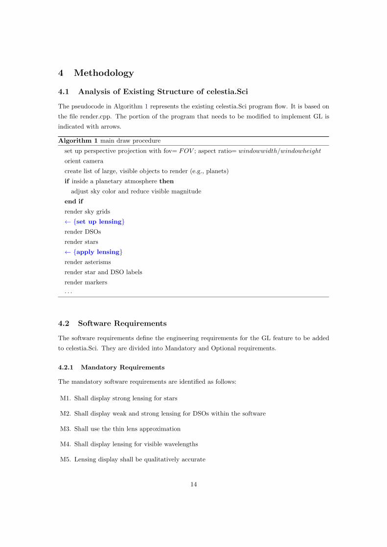
4.1 Analysis of Existing Structure of celestia.Sci

The pseudocode in Algorithm 1 represents the existing celestia.Sci program flow. It is based on

the file render.cpp. The portion of the program that needs to be modified to implement GL is

indicated with arrows.

Algorithm 1 main draw procedure

set up perspective projection with fov= FOV ; aspect ratio= windowwidth/windowheight

orient camera

create list of large, visible objects to render (e.g., planets)

if inside a planetary atmosphere then

adjust sky color and reduce visible magnitude

end if

render sky grids

← set up lensingrender DSOs

render stars

← apply lensingrender asterisms

render star and DSO labels

render markers

· · ·

4.2 Software Requirements

The software requirements define the engineering requirements for the GL feature to be added

to celestia.Sci. They are divided into Mandatory and Optional requirements.

4.2.1 Mandatory Requirements

The mandatory software requirements are identified as follows:

M1. Shall display strong lensing for stars

M2. Shall display weak and strong lensing for DSOs within the software

M3. Shall use the thin lens approximation

M4. Shall display lensing for visible wavelengths

M5. Lensing display shall be qualitatively accurate

14

M5.1. Shall display lensing from arbitrary orientations

M5.2. Shall lens light from stars and deep sky objects

M5.3. Shall magnify brightness

M5.4. Shall be able to display Einstein rings

M5.5. Shall be able to display multiple images

M5.6. Shall be able to display distorted (sheared/rotated) arclets

M5.7. Shall be able to display lensing contributions from multiple neighboring masses

M6. Shall not affect existing functionality

M7. Shall not decrease frame rates below interactive levels (at least 10 fps)

4.2.2 Optional Requirements

The optional, or extended software requirements (to be implemented as time permits) are iden-

tified as follows:

O1. Shall be able to toggle on/off easily during program operation

O2. Shall be able to observe lensing from within a planetary atmosphere

O3. Shall plot the microlensing light curve for exoplanets as a graph in real time

4.3 Software Specifications

4.3.1 A Brief Overview of the OpenGL Pipeline

The graphics engine of celestia.Sci is implemented using OpenGL, a popular 3d API (application

programming interface). More specifically, repetitive graphical functionality which incurs high

computational cost such as rendering stars and galaxies is implemented as OpenGL GPU shaders.

An extensive discussion of OpenGL and GPU shaders is beyond the scope of this report, and

here we will only explain the aspects salient to our implementation of GL.

Figure 9 illustrates the OpenGL pipeline, or how 3d geometric data and images (textures)

are processed by computer graphics hardware into frames, or images in an animated sequence.

Here, we are mainly interested in GPU shaders. Shaders are specialized programs that run

highly parallelized, either on the vertex processor or the fragment processor to process vertices

(geometry) or fragments (roughly equivalent to pixels).

4.3.2 Why Exploit the Fragment Processor?

The fragment processor is particularly interesting to us, because each fragment in essence rep-

resents a light ray originating from within the simulation, regardless of whether the light source

15

!!

(Geometry)!!

App!Memory!

!!!!!!

(Pixels)!!!!!!

Vertex&Processor&

Primi3ve!Assembly!

Clip!Project!Viewport!

Cull!

Pixel!Unpack!

Pixel!Transfer!

Pixel!Pack!

(Geometry)!!

Rasterize!!!!

(Pixels)!

Fragment&Processor&

Per!Fragment!Opera3ons!

Frame!Buffer!

Opera3ons!

Frame!Buffer!

Read!Control!

Texture!Memory!

Pixel!Groups!Ver3ces!

Fragments!Textures!

Programmable!Processor!

Figure 9: OpenGL shader pipeline (figure adapted from Rost et al., 2006)

is a star or a galaxy. Thus a fragment shader will process all sources of light in the scene demo-

cratically, and at the resolution of the final image. This is equivalent to computing the lensing

deflection angle (Equation 11) on a grid of dimensions equivalent to the rendered image.

Additionally, we use a two-pass approach shown in Figure 10 where we first render stars and

DSOs to a texture in memory using a framebuffer object (FBO). Then we draw the texture as a

quad covering the entire window. We apply a lensing fragment shader during this second step.

4.3.3 Coordinate Transforms

A major challenge in this strategy is to correctly transform coordinates between texture space,

where the lensing effect is calculated in the fragment shader, and world space. Distances in the

lens equation 14 must be computed in world units (km), and the angular deflection (11) must be

converted to a displacement in texture units. Table 1 summarizes the transform requirements:

Quantity Source Coordinate Space → Destination Space

impact parameter |ξ| Texture World

displacement amount Ddsα World Texture

center of lensing mass World Texture

Table 1: Coordinate transform requirements

One issue with computing the displacement amount Ddsα is that Dds is unknown inside the

fragment shader; in fact at this stage we do not know the specific coordinates of the stars and

DSOs that were rendered to the texture any more. This is the reason why one of the inputs to

16

Light&rays&from&&stars&and&DSOs&

FBO&

Full7screen&quad&&(lens&fragment&shader&runs&here)&

Visible&area&&(window)&

Figure 10: Two-pass render strategy using a FBO

the fragment shader must be the center of the lensing mass in texture coordinates; Dds on the

other hand is expensive to store or recompute for each source star/DSO. We choose instead to

use a similar approximation as Weiskopf et al. (2005), and set Dds = a constant large value (light

years) as Dds is already a large value for most sources and thus any distance variation between

sources will have a vanishing impact on Ddsα.

To implement the coordinate transforms, it is necessary to keep in mind that OpenGL im-

plements three intermediate coordinate spaces between world (object) space and texture space.

These are the eye, clip and normalized device coordinate (NDC) spaces. Figure 11 illustrates

the standard OpenGL coordinate transform flow from geometry to the window. In our case,

we require a final, additional transform from texture space to window space. As texture space

is square (0, 0) − (1, 1) while window space is generally not, we must render to horizontally or

vertically distorted coordinates depending on the aspect ratio of the window, then “undistort”

when rendering to the full-screen quad in window space.

4.3.4 Rejected Approach

Another approach that was considered and rejected, was to notice that space is usually sparsely

populated with objects such as stars and galaxies; thus a geometric lensing deformation might

be applied to individual objects at the vertex processor level to potentially reduce the number

of lensing computations required. However, this method requires that each object be composed

of enough vertices to allow realistic deformation into arcs and rings; with thousands of stars

and galaxies within the simulation, the large number of vertices required could swamp the vertex

processor. Also, this method will fail to work when lensing becomes sufficiently strong to produce

17

MODELVIEW)Matrix)

object'space'

PROJECTION)Matrix)

Perspec9ve)Divide)

Viewport/Depth)range)scale)and)bias)

eye'space'

vertex)posi9on)

clip'space'

normalized'device'coordinate'space'

window'space'

window)coordinate)

Figure 11: OpenGL coordinate transforms (figure adapted from Rost et al., 2006)

multiple images. This is because it is impossible for a vertex shader to generate new vertices.

More recent versions of the OpenGL API are able to access additional programmable processors

that can generate new vertices, but celestia.Sci is not compatible yet with these API versions.

4.3.5 Calculating Mass

In Section 2, we briefly touched on calculating masses from luminosities using the mass-to-light

ratio (M/L). At scales smaller than clusters, M/L varies according to the scale of the object.

We thus describe the relations used in this report for each class of object.

Stars

Stellar mass can be estimated from luminosity using data compiled by Torres et al. (2009).

Figure 12 shows a plot of all of the data, where we have performed piecewise linear fits.

Based on the fitted powers n, the relations we use to derive mass M from luminosity L are

given in Table 2.

L < 0.006 L L/L = (M/M)4

L < 0.016 L L/L = (M/M)3.76

L < 51 L L/L = (M/M)4.46

L < 1.5× 105 L L/L = (M/M)3.32

L ≥ 1.5× 105 L M/L ∼ 1

Table 2: Stellar mass-to-light ratios

18

n = 3.32

n = 4.46

n = 3.76 n = 4.00

-­‐4

-­‐2

0

2

4

6

-­‐1 -­‐0.5 0 0.5 1 1.5

log L/L

log M/M

Figure 12: Mass-to-light ratios for stars (Torres et al., 2009). Fits have been added.

Galaxies

For galaxies, M/L depends on the galaxy type (spiral, irregular, elliptical). We use the approx-

imate values adopted by Bahcall and Kulier (2014) that are based on the Milky Way M/L for

spiral and elliptical types, and the typical value for irregular types quoted by Carroll and Ostlie

(2007). The following table summarizes the M/L values used in this project:

Spiral Elliptical (E/S0)* Irregular

100 200 1

Table 3: Mass-to-light ratios per galaxy type in M/L units

*For elliptical types, mass and luminosity are not linear but rather are related to the radius

R and velocity dispersion σ by a power law (M/L)0.8 ∝ (Rσ2/L) (Bernardi et al., 2003). For

simplicity, we assume linearity but a more rigorous treatment should keep this in mind.

Galaxy Clusters

At the scale of clusters (> 300 h−1 Mpc), the mass-to-light (M/L) ratio was shown to be

409± 29 h M/L where h = 0.7 (Bahcall and Kulier, 2014).

Exoplanets

Exoplanet masses are already given in the celestia.Sci exoplanet database and do not need to be

computed.

19

4.3.6 General Lensing Framework

A general lensing framework for celestia.Sci must be able to handle all possible type of stars

and DSOs regardless of luminosities, ellipticities and presence of orbiting objects as well as the

viewing orientation and FOV.

Stellar Lensing

Algorithm 2 represents the pseudocode for a stellar lensing shader (refer to Appendix A for the

full shader code listing). Algorithm 3 describes how the shader functions within celestia.Sci.

Algorithm 2 Stellar lensing fragment shader

massPosTexCoord← lensing mass position in texture space

massDist← Dd

massRadius← radius of lensing mass in world units

for all fragments do

n ← (massPosTexCoord − 〈s, t〉) s, t are texture coordinates sampled at the current

fragmentp← |n| in texture units

r ← max(massRadius, 2 ∗massDist ∗ p)|A| ← 1/(1− θ4

E/θ4)

α← 4 ∗G ∗M/(c2 ∗ r)deyespace ← 〈|n| ∗ α ∗ large distance,−large distance, 1.0〉dNDC ← deyespace projected into NDC space

fragment color ← |A|∗sample from texture at dNDC

end for

Galactic Lensing

There are two major galactic lensing scenarios: galaxy-galaxy and cluster lensing. Galaxy lensing

can be modeled very similarly to stellar lensing. However, cluster lensing requires summing at

every fragment the contribution to the amount of deflection from each galaxy inside the cluster.

For this project, we implemented a naıve O(n2) algorithm where the summation is repeated for

every fragment and restricted to 50 galaxies at a time. A more efficient scheme might cache the

lensing contributions of each galaxy and potentially cull contributions based on distance.

Microlensing

Microlensing requires an entirely different approach. Not only is there no perceptible geometric

deflection of light, but also there must be a way to sample the light curve and display it in a

separate graph. Additionally, there are two (or more) lensing masses and the superposition must

be modeled.

20

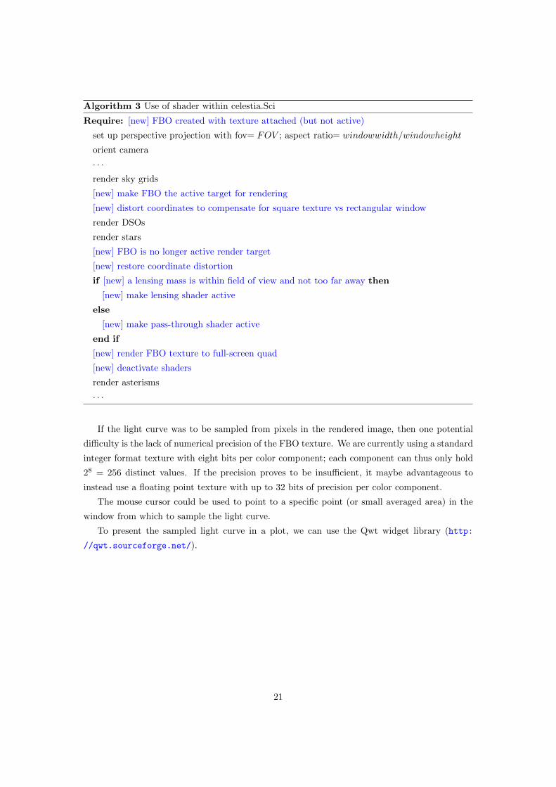
Algorithm 3 Use of shader within celestia.Sci

Require: [new] FBO created with texture attached (but not active)

set up perspective projection with fov= FOV ; aspect ratio= windowwidth/windowheight

orient camera

· · ·render sky grids

[new] make FBO the active target for rendering

[new] distort coordinates to compensate for square texture vs rectangular window

render DSOs

render stars

[new] FBO is no longer active render target

[new] restore coordinate distortion

if [new] a lensing mass is within field of view and not too far away then

[new] make lensing shader active

else

[new] make pass-through shader active

end if

[new] render FBO texture to full-screen quad

[new] deactivate shaders

render asterisms

· · ·

If the light curve was to be sampled from pixels in the rendered image, then one potential

difficulty is the lack of numerical precision of the FBO texture. We are currently using a standard

integer format texture with eight bits per color component; each component can thus only hold

28 = 256 distinct values. If the precision proves to be insufficient, it maybe advantageous to

instead use a floating point texture with up to 32 bits of precision per color component.

The mouse cursor could be used to point to a specific point (or small averaged area) in the

window from which to sample the light curve.

To present the sampled light curve in a plot, we can use the Qwt widget library (http:

//qwt.sourceforge.net/).

21

5 Results and Analysis

5.1 Exercise: Our Sun

Figure 13 is a frame capture from celestia.Sci, illustrating the lensing code.

Figure 13: Lensing of a star as seen near our Sun, simulated using celestia.Sci. The corona has

been hidden for clarity. The lensed image is superimposed over the unlensed source.

The frame rate of celestia.Sci (Figure 14) in this sparsely populated scene is approximately 60

fps, which satisfies our criteria for interactivity. The hardware is an Apple MacBook Air laptop

with 1.6 GHz CPU, 4 GB RAM and Intel HD Graphics 3000 integrated GPU (information given

in “About This Mac”). The operating system is Mac OS X 10.9.2.

As an independent confirmation of the frame rate, Apple’s OpenGL Driver Monitor software

was used to monitor buffer swap count per second (Figure 14).

0

20

40

60

80

100

120

140

0 10 20 30 40 50 60 70 80 90 100 110

Buffe

r Swap Cou

nt/s

Time

Figure 14: Buffer swap count per second (equivalent to frame rate×2). Cel url:

cel://Follow/Sol/2014-01-21T16:43:48.45332?x=AICxE/dvzJ8D&y=AIDovwJclyEM&z=

AIDFnLyE+5cJ&ow=-0.335985&ox=-0.276615&oy=-0.345776&oz=-0.831286&select=Sol&

fAM45=5.1&fov=0.0207504&ts=1&ltd=0&p=0&rf=135806977&lm=2068&ig=0&tsrc=0&ver=3

22

Buffer swap count is normally equal to the frame rate, but the OpenGL implementation

used by celestia.Sci (QGLWidget, part of the Qt 4.8 software framework) uses double buffering

and this artificially causes the number of buffer swaps to be 60 × 2 = 120. During the test,

the celestia.Sci window was made full screen (1366×768 resolution), and interactions such as

zooming, panning and rotating were performed. The buffer swap count is seen to dip briefly to

60 (30 fps); this corresponds to a galaxy becoming visible due to view rotation.

We now proceed to reproduce the eclipse of 1919 in celestia.Sci. Figure 15 shows our result.

(a) The eclipse of 1919 in celestia.Sci (b) Zoomed in view of star

(c) Schematic of Eddington’s eclipse ob-

servations (Dyson et al., 1920). Arrow in-

dicates zoomed portion in celestia.Sci

Figure 15: Simulating the 1919 solar eclipse in celestia.Sci

celestia.Sci has an eclipse finding feature that allows us to go back in time and precisely

simulate the eclipse. The arrangement of stars in the simulation can be seen to match those

observed by Eddington. Figure 15b magnifies a star very close to the corona; again we have

superimposed the lensed image over the unlensed star. The diameter in pixels of the Sun in

Figure 15b is 1100 pixels. Given the known angular diameter of the Sun = 1914′′, and the

expected angular separation between the lensed and unlensed images ∼ 1.75′′, we can expect

23

the separation between the images to be = 1914/1.75/1100 ∼ 0.99 pixels. The actual separation

between the two simulated images, as measured by visual inspection, is 1 pixel as expected.

5.2 Exercise: Coma Galaxy Cluster

We now turn our attention to GL at the cosmological scale of a galaxy cluster. While catalog

data for distant clusters such as the Bullet Cluster is not available in celestia.Sci, the Coma

Cluster (Abell 1656) is another good candidate for testing our lensing code due to the presence

of two very massive BCGs (brightest central galaxies) NGC 4874 and NGC 4889. Additionally,

the cluster is near our own galaxy and thus reliable catalog data is available within celestia.Sci.

Figure 16 shows the result of our lensing simulation in celestia.Sci.

(a) Simulated lensing in the Coma Cluster (b) Zoomed view

(c) Coma Cluster (Sloan Digital Sky Survey, n.d)

Figure 16: The Coma Cluster.

Several characteristics of strong and weak lensing can be seen near NGC 4874 (large galaxy

in the upper right of Figure 16a and magnified in Figure 16b): arclets, multiple images and the

24

emergence of a ring-like structure. In fact the feature is an Einstein ring, as can be seen in

Figure 17 where the apparent magnitudes in the scene have been artificially boosted. Note that

the center of the distortion is not located at the centers of any of the BCGs or the midpoints

between them; qualitatively, this is to be expected due to the asymmetric mass distribution.

Figure 17: Einstein ring in the Coma Cluster, generated by our code.

Figure 18 represents the buffer swap count measured for the Coma Cluster scene (as usual,

we have to divide by 2 to obtain the frame rate). The minimum frame rate in this complex scene

is ∼ 10 fps, which is the absolute minimum that we require for interactivity.

0

20

40

60

80

100

120

0 10 20 30 40 50 60 70

Buffe

r Swap Cou

nt/s

Time

Figure 18: Buffer swap count per second measured for lensing in the Coma Cluster. Cel url for

reproduction: cel://Follow/NGC%204889/2014-04-10T23:26:44.68594?x=AAAAAAAAAAhN+

tBofLr//w&y=AAAAAAAAANKmRt0+FSo&z=AAAAAAAAYL2CJexFegE&ow=0.253613&ox=0.687271&

oy=-0.128477&oz=-0.668455&select=NGC%204874&fAM45=14&fov=0.662792&ts=1&ltd=0&p=

0&rf=68960535&lm=2064&ig=0&tsrc=0&ver=3

25

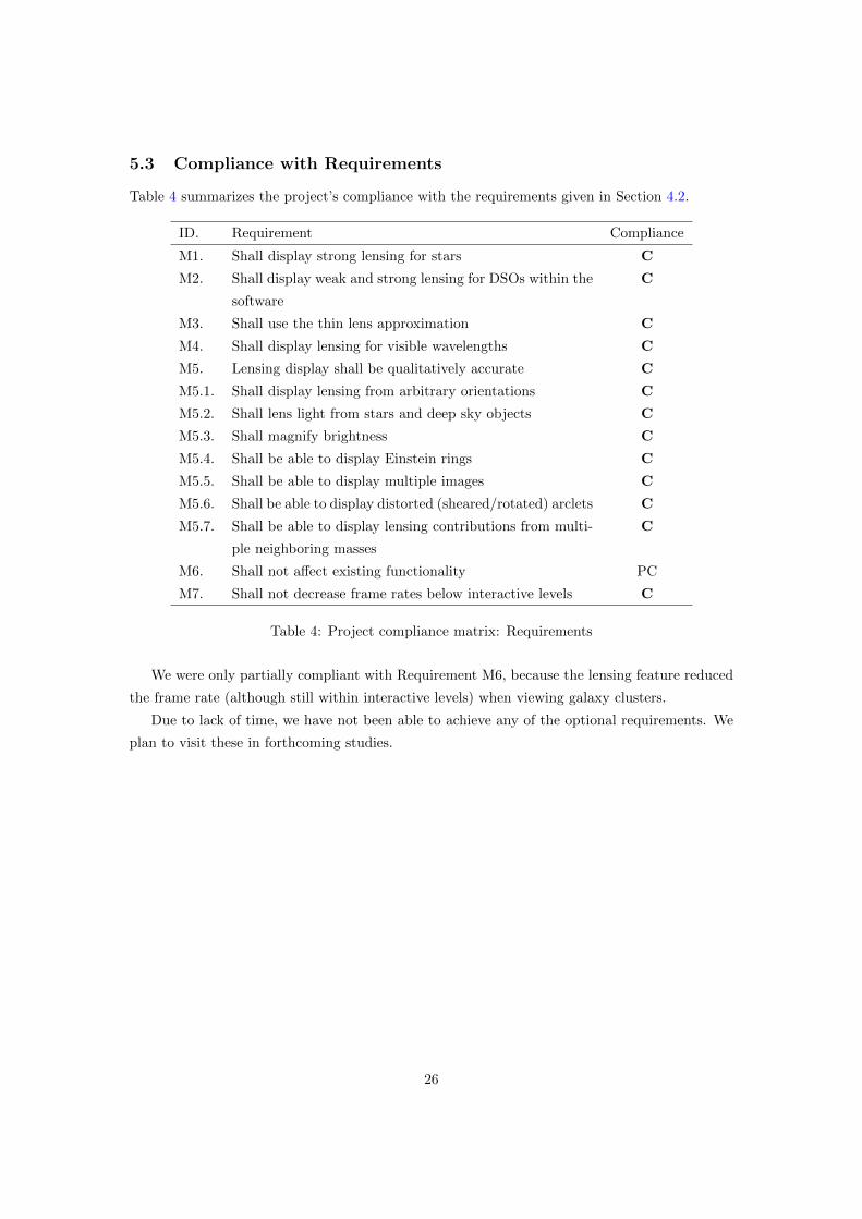
5.3 Compliance with Requirements

Table 4 summarizes the project’s compliance with the requirements given in Section 4.2.

ID. Requirement Compliance

M1. Shall display strong lensing for stars C

M2. Shall display weak and strong lensing for DSOs within the

software

C

M3. Shall use the thin lens approximation C

M4. Shall display lensing for visible wavelengths C

M5. Lensing display shall be qualitatively accurate C

M5.1. Shall display lensing from arbitrary orientations C

M5.2. Shall lens light from stars and deep sky objects C

M5.3. Shall magnify brightness C

M5.4. Shall be able to display Einstein rings C

M5.5. Shall be able to display multiple images C

M5.6. Shall be able to display distorted (sheared/rotated) arclets C

M5.7. Shall be able to display lensing contributions from multi-

ple neighboring masses

C

M6. Shall not affect existing functionality PC

M7. Shall not decrease frame rates below interactive levels C

Table 4: Project compliance matrix: Requirements

We were only partially compliant with Requirement M6, because the lensing feature reduced

the frame rate (although still within interactive levels) when viewing galaxy clusters.

Due to lack of time, we have not been able to achieve any of the optional requirements. We

plan to visit these in forthcoming studies.

26

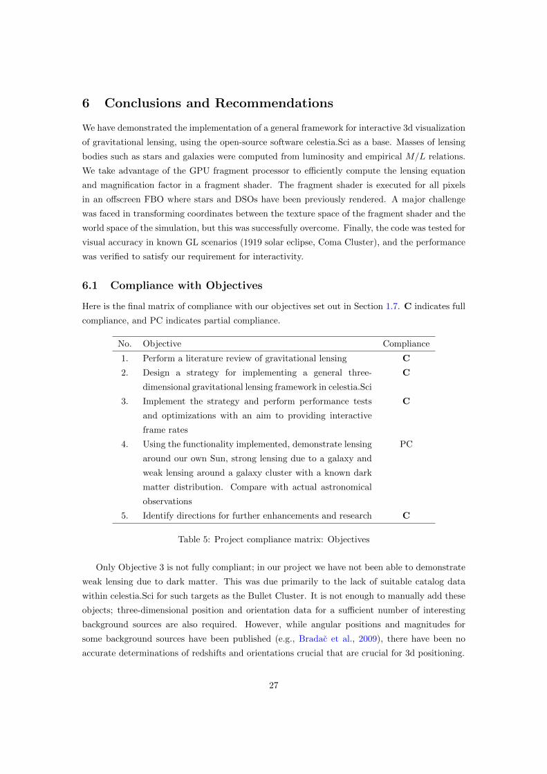
6 Conclusions and Recommendations

We have demonstrated the implementation of a general framework for interactive 3d visualization

of gravitational lensing, using the open-source software celestia.Sci as a base. Masses of lensing

bodies such as stars and galaxies were computed from luminosity and empirical M/L relations.

We take advantage of the GPU fragment processor to efficiently compute the lensing equation

and magnification factor in a fragment shader. The fragment shader is executed for all pixels

in an offscreen FBO where stars and DSOs have been previously rendered. A major challenge

was faced in transforming coordinates between the texture space of the fragment shader and the

world space of the simulation, but this was successfully overcome. Finally, the code was tested for

visual accuracy in known GL scenarios (1919 solar eclipse, Coma Cluster), and the performance

was verified to satisfy our requirement for interactivity.

6.1 Compliance with Objectives

Here is the final matrix of compliance with our objectives set out in Section 1.7. C indicates full

compliance, and PC indicates partial compliance.

No. Objective Compliance

1. Perform a literature review of gravitational lensing C

2. Design a strategy for implementing a general three-

dimensional gravitational lensing framework in celestia.Sci

C

3. Implement the strategy and perform performance tests

and optimizations with an aim to providing interactive

frame rates

C

4. Using the functionality implemented, demonstrate lensing

around our own Sun, strong lensing due to a galaxy and

weak lensing around a galaxy cluster with a known dark

matter distribution. Compare with actual astronomical

observations

PC

5. Identify directions for further enhancements and research C

Table 5: Project compliance matrix: Objectives

Only Objective 3 is not fully compliant; in our project we have not been able to demonstrate

weak lensing due to dark matter. This was due primarily to the lack of suitable catalog data

within celestia.Sci for such targets as the Bullet Cluster. It is not enough to manually add these

objects; three-dimensional position and orientation data for a sufficient number of interesting

background sources are also required. However, while angular positions and magnitudes for

some background sources have been published (e.g., Bradac et al., 2009), there have been no

accurate determinations of redshifts and orientations crucial that are crucial for 3d positioning.

27

6.2 Recommendations for Further Research

Here is a list of recommendations for further research.

1. Pursue the optional objectives given in Section 1.7, and fulfill the optional requirements

listed in Section 4.2.2. These include, for example, implementing microlensing of exoplanets

and developing a companion workshop;

2. Refine the mass estimation method for elliptical galaxies;

3. Improve the performance of computing GL systems with multiple components (e.g., galaxy

clusters) via memory caching techniques;

4. Test with more extensive DSO catalog data as they become available.

28

References

Bahcall, N. A. and Kulier, A., 2014. Tracing Mass and Light in the Universe: Where is the Dark

Matter? MNRAS, 439(3), pp.2505–2514.

Bernardi, M., and et al., 2003. Early-Type Galaxies in the Sloan Digital Sky Survey. III. The

Fundamental Plane. The Astronomical Journal, 125(4), pp.1866–1881.

Bradac, M., and et al., 2009. Focusing Cosmic Telescopes: Exploring Redshift z ˜ 5-6 Galaxies

with the Bullet Cluster 1E0657 – 56. The Astrophysical Journal, 706(2), pp.1201–1212.

Carroll, B. W. and Ostlie, D. A., 2007. An Introduction to Modern Astrophysics, 2nd ed. San

Francisco, CA: Addison-Wesley.

Clowe, D., and et al., 2006. A Direct Empirical Proof of the Existence of Dark Matter. The

Astrophysical Journal Letters, 648, pp.L109–L113.

Coe, D., and et al., 2010. A High-Resolution Mass Map of Galaxy Cluster Substructure: LensPer-

fect Analysis of A1689. The Astrophysical Journal, 723(2), pp.1678–1702.

Dyson, F. W., and et al., 1920. A Determination of the Deflection of Light by the Sun’s Grav-

itational Field, from Observations Made at the Total Eclipse of May 29, 1919. Philosoph-

ical Transactions of the Royal Society A: Mathematical, Physical and Engineering Sciences,

220(571-581), pp.291–333.

ESA, 2004. Closing in on the Red Planet: Mars Express orbit lowered. Available

from: <http://www.esa.int/Our_Activities/Space_Science/Mars_Express/Closing_

in_on_the_Red_Planet_Mars_Express_orbit_lowered>[Accessed 21 November 2013].

ESA/Hubble and NASA, 2012. Seeing quadruple. Available from: <http://

www.spacetelescope.org/static/archives/images/screen/potw1204a.jpg>[Accessed 21

November 2013].

Gavazzi, R., and et al., 2008. The Sloan Lens ACS Survey. VI. Discovery and Analysis of a

Double Einstein Ring. The Astrophysical Journal, 677(2), pp.1046–1059.

King, L. J., and et al., 1998. A complete infrared Einstein ring in the gravitational lens system

B1938 + 666. Monthly Notices of the Royal Astronomical Society, 295(2), pp.L41–L44.

Kneib, J. P., and et al., 1996. Hubble Space Telescope Observations of the Lensing Cluster Abell

2218. The Astrophysical Journal, pp.643–656.

Lefor, A. T., and et al., 2013. A systematic review of strong gravitational lens modeling software.

New Astronomy Reviews, 57(1-2), pp.1–13.

Maccone, C., 1999. Tethered system to get magnified radio pictures of the Galactic Center from

a distance of 550 AU. Acta Astronautica, 45(2), pp.109–114.

29

Magallon, M. and Paez, J., 2002. Abstract Interactive Visualization of Gravitational Lenses.

In: G. Greiner, H. Niemann, T. Ertl, B. Girod, and H. P. Seidel Eds., Vision, Modeling, and

Visualization 2002. IOS Press.

Mao, S. and Paczynski, B., 1991. Gravitational microlensing by double stars and planetary

systems. Astrophys. J. Lett., 374, pp.L37–L40.

Narayan, R. and Bartelmann, M., 1997. Lectures on Gravitational Lensing.

NASA, 2004. NASA: Solar System Website and Celestia Software. Available

from: <http://teachspacescience.org/cgi-bin/search.plex?catid=10000913&mode=

full>[Accessed 21 November 2013].

NASA, and et al., 2008. Hubble Finds Double Einstein Ring. Available from: <http:

//hubblesite.org/newscenter/archive/releases/2008/04/image/a/>[Accessed 1 April

2014].

Natario, J., 2012. General Relativity Without Calculus - A Concise Introduction to the Geometry

of Relativity. Available from: <http://www.math.ist.utl.pt/~jnatar/RM-12/Geom_Rel.

pdf>[Accessed 19 November 2013].

Planck Collaboration, 2014. Planck 2013 results. XVI. Cosmological parameters. arXiv, preprint.

Available from: <http://arxiv.org/abs/1303.5076>[Accessed 25 March 2014].

Rost, R. J., and et al., 2006. OpenGL Shading Language, 2nd ed. Upper Saddle River,

NJ: Addison-Wesley.

Saha, P., 2000. Gravitational Lensing. In: P. Murdin Ed., Encyclopedia of Astronomy and

Astrophysics, pp.1–8. Bristol: Institute of Physics Publishing.

Schneider, P., and et al., 1992. Gravitational Lenses. Berlin, Heidelberg, New York: Springer-

Verlag.

Schneider, P., and et al., 2006. Gravitational Lensing: Strong, Weak and Micro. Berlin, Heidel-

berg, New York: Springer.

Schrempp, F., 2013. Welcome: Aims and Status of celestia.Sci. Available from: <http://

forum.celestialmatters.org/viewtopic.php?f=11&t=473>[Accessed 21 November 2013].

Sloan Digital Sky Survey, n.d. Coma Cluster. Available from: <http://www.sdss.org/iotw/

coma.jpg>[Accessed 11 April 2014].

Spergel, D. N., and et al., 2007. Three-Year Wilkinson Microwave Anisotropy Probe (WMAP)

Observations: Implications for Cosmology. The Astrophysical Journal Supplement Series,

170(2), pp.377–408.

30

Torres, G., and et al., 2009. Accurate masses and radii of normal stars: modern results and

applications. The Astronomy and Astrophysics Review, 18(1-2), pp.67–126.

Walsh, D., and et al., 1979. 0957 + 561 A, B: twin quasistellar objects or gravitational lens?

Nature, 279(5712), pp.381–384.

Weiskopf, D., and et al., 2005. Visualization in the Einstein Year 2005: a case study on explana-

tory and illustrative visualization of relativity and astrophysics. In: Visualization, 2005. VIS

05. IEEE, pp.583–590. IEEE.

Weiskopf, D., and et al., 2004. GPU-Based Nonlinear Ray Tracing. Computer Graphics Forum,

23(3), pp.625–633.

31

Appendix A Shader Code

Listing A1: Stellar lensing fragment shader

uniform sampler2D tex;

uniform float mass[10];

uniform vec2 massPosTexCoord[10];

uniform float massDist[10];

uniform float massRadius[10];

uniform vec2 windowSize;

uniform float pixelSize ;

uniform float LARGE DISTANCE;

void main(void) vec2 texCoordFinal = gl TexCoord[0].st;

vec2 normal = (massPosTexCoord[0] − texCoordFinal);

vec2 normalizedNormal = normalize(normal);

float p = windowSize.y∗length(normal);

float r = max(massRadius[0], 2.0∗massDist[0]∗p∗pixelSize);

float alpha = 5.91∗mass[0]/r; //5.91=4GM sun/cˆ2 in km

float thetaE2 = 5.91∗mass[0]/massDist[0];

float magnification = 1.0/(1.0−thetaE2∗thetaE2/pow(r/massDist[0], 4.0));

float amountEye = alpha ∗ LARGE DISTANCE;

vec4 deflectEye = vec4(normalizedNormal∗amountEye, −5.0, 1.0);

vec4 deflectNDC = gl ProjectionMatrix∗deflectEye;

deflectNDC /= deflectNDC.w;

texCoordFinal += deflectNDC.xy;

gl FragColor = magnification ∗ texture2D(tex, texCoordFinal);

32

Appendix B Plot Code

Listing B1: GNU Octave code for Figure 7

%colormapRGBmatrices function taken from:

%http://cresspahl.blogspot.fr/2012/03/expanded−control−of−octaves−colormap.html

function mymap = colormapRGBmatrices(N, rm, gm, bm)

x = linspace(0,1, N);

rv = interp1( rm(:,1), rm(:,2), x);

gv = interp1( gm(:,1), gm(:,2), x);

mv = interp1( bm(:,1), bm(:,2), x);

mymap = [ rv’, gv’, mv’];

%exclude invalid values that could appear

mymap( isnan(mymap) ) = 0;

mymap( (mymap>1) ) = 1;

mymap( (mymap<0) ) = 0;

end

M = [0,1;0.05,1;1,0];

invgray = colormapRGBmatrices(256, M, M, M);

Dd=1.5.∗10ˆ8;

Dds=9.5.∗10ˆ13;

Ds=Dds+Dd;

thetaE2=5.91.∗Dds./(Dd.∗Ds);

f = @(x,y) 1./(1 .− thetaE2.ˆ2 ./ (sqrt((x.∗69600).ˆ2+(y.∗69600).ˆ2) ./ Dd).ˆ4);

d = −2.5:0.01:2.5;

[X,Y] = meshgrid(d,d);

Z = f(X,Y);

Z((X.ˆ2+Y.ˆ2)<1.0) = 1.0;

hold on

[c,h] = contourf(X,Y,Z,100);

set(h ,’EdgeColor’,’none’);

set(gca, ’Position ’, [0.14 0.14 0.75 0.8]);

xlabel (’x/R sun’);ylabel (’y/R sun’);colormap(invgray);

colorbar;

hold off

33

Listing B2: GNU Octave code for Figure 8

hold on

xlabel (’( t−t 0)/t E’);

ylabel (’Magnification ’);

t=−1.0:0.001:1.0;

global u0;

for u0=0.01:0.01:0.1;

A=(t.ˆ2+u0ˆ2+2)./((t.ˆ2+u0ˆ2).ˆ0.5.∗(t.ˆ2+u0ˆ2+4).ˆ0.5);

Aq=interp1(t,A,t,’spline ’);

plot(t ,Aq);

end;

hold off

34