Copyright © 2014 by Robert Lagerström, Carliss Baldwin, Alan MacCormack, and David Dreyfus

Working papers are in draft form. This working paper is distributed for purposes of comment and discussion only. It may not be reproduced without permission of the copyright holder. Copies of working papers are available from the author.

Visualizing and Measuring Software Portfolio Architectures: A Flexibility Analysis Robert Lagerström Carliss Baldwin Alan MacCormack David Dreyfus

Working Paper

14-083 March 4, 2014

2

Abstract

In this paper, we test a method for visualizing and measuring software portfolio

architectures, and use our measures to predict the costs of architectural change. Our data

is drawn from a biopharmaceutical company, comprising 407 architectural components

with 1,157 dependencies between them. We show that the architecture of this system can

be classified as a “core-periphery” system, meaning it contains a single large dominant

cluster of interconnected components (the “Core”) representing 32% of the system. We

find that the classification of software applications within this architecture, as being

either Core or Peripheral, is a significant predictor of the costs of architectural change.

Using OLS regression models, we show that this measure has greater predictive power

than prior measures of coupling used in the literature.

Keywords: Design structure matrices, Software architecture, Flexibility, and Software application portfolio

3

1. INTRODUCTION

Contemporary business environments are constantly evolving, requiring continual

changes to the software applications that support a business. Moreover, during recent

decades the sheer number of applications has grown significantly, and they have become

increasingly interdependent. As a result, the management of software applications has

become a complex task; many companies find that implementing changes to their

application portfolio architecture is increasingly difficult and expensive. To help manage

this complexity, firms need a way to visualize and analyze the modularity of their

software portfolio architectures and the degree of coupling between components.

(Baldwin et al., 2013) present a method to visualize the hidden structure of

software architectures based on Design Structure Matrices (DSMs) and classic coupling

measures. This method has been tested on numerous software releases for individual

applications (such as Linux, Mozilla, Apache, and GnuCash) but not on software

portfolio architectures in which a large number of interdependent applications have

relationships with other types of components such as business groups and/or

infrastructure elements. In contrast, (Dreyfus and Wyner, 2011) have mapped

dependencies across the enterprise architecture of a biopharmaceutical company (referred

to as BioPharma), which includes a large portfolio of software applications. In this paper,

we apply Baldwin et. al.’s architectural visualization and measurement methods to

enterprise architecture, using the data collected by (Dreyfus, 2009). This data comprises

407 architectural components, of which 191 are software applications; and 1,157

dependencies, of which 494 are between these software applications.

We show that the biopharmaceutical firm’s enterprise architecture can be

classified as core-periphery. This means that 1) there is one cyclic group (the “Core”) of

components that is substantially larger than the second largest cyclic group, and 2) this

group comprises a substantial portion of the entire architecture. We find that the Core

contains 132 components, representing 32% of the architecture. Furthermore, we show

that the Core contains only software applications, whereas the business and infrastructure

components are classified as either Control, Shared, or Peripheral elements. Finally, we

show that the architecture has a propagation cost of 23%, meaning almost one-quarter of

the system may be affected when a change is made to a randomly selected component.

4

Following (Dreyfus, 2009), we pay special attention to the software portfolio

architecture and the categorization of software applications as either Core or Periphery.

We test the hypothesis that the classification of software applications is correlated with

architectural flexibility (operationalized as the cost of change estimated by IT Service

Owners). Our analysis makes use of both Pearson correlations and OLS regression

models with controls. We find that the classification of applications in the architecture

(as being in the Core or the Periphery) is significantly correlated with architectural

flexibility. In statistical tests, we show that this measure has greater predictive power than

prior measures of coupling used in the literature.

The paper is structured as follows: Section 2 presents related work; Section 3

describes the hidden structure method; Section 4 presents the biopharmaceutical case

used for the analysis; Section 5 describes the statistical tests that were conducted; Section

6 discusses our results; Section 7 outlines future work; and Section 8 concludes the paper.

2. RELATED WORK

In this section, we first describe the most common metrics used to assess

complexity in software engineering. These metrics are typically used to help analyze a

single software component or system in order that, for example, managers can estimate

development effort or programmers can identify troublesome code. We follow this by

describing recent work on the visualization and measurement of complex software

architectures. These network approaches have emerged because many software

applications have grown into large systems containing thousands of interdependent

components, making it difficult for a designer to grasp the full complexity of the design.

2.1 Software engineering metrics

According to (IEEE Standards Board, 1990), software complexity “is the degree

to which a system or component has a design or implementation that is difficult to

understand and verify.” In software engineering, metrics to measure complexity have

existed for many years. Among the earliest are Lines Of Code (LOC) and Function

Points (FP) — metrics that measure the size of a program, often used as a proxy for

complexity (Laird and Brennan, 2006). FP analysis is based on the inputs, outputs,

5

interfaces and databases in a system. LOC can be measured in different ways: by

counting every line of code (SLOC) or restricting attention to non-commented lines of

code (NLOC) or logical lines of code (LLOC) where only the executable statements are

counted. Since different programming languages are more or less expressive per line of

code, a gearing factor can be used to assist in comparisons of software written in different

languages. However, given LOC and FP do not capture the relationships between

components in a system, and focus only on size, they are at bests proxies for complexity.

One of the first complexity metrics proposed and widely used today is McCabe's

Cyclomatic Complexity (MCC), which is based on the control structure of a software

component. The control structure can be expressed as a control graph in which the

cyclomatic complexity value of a software component can be calculated (McCabe, 1976).

A year later, another well-known metric was introduced, namely, Halstead's complexity

metric (Halstead, 1977), which is based on the number of operators (e.g., “and,” “or,” or

“while”) and operands (e.g., variables and constants) in a software component.

Subsequently, the Information Flow Complexity (IFC) metric was introduced (Henry and

Kafura, 1981). IFC is based on the idea that a large amount of information flow in a

system is caused by low cohesion, which in turn results in high complexity.

Recent work in this field has tended to focus on measuring coupling as a way to

capture complexity (Stevens et al., 1974) (Chidamber and Kemerer, 1994). (IEEE

Standards Board, 1990) defines coupling as “the manner and degree of interdependence

between software modules. Types include common-environment coupling, content

coupling, control coupling, data coupling, hybrid coupling, and pathological coupling.”

According to (Chidamber and Kemerer, 1994), excessive coupling is detrimental to

modular design and prevents the reuse of objects in a codebase.

(Fenton and Melton, 1990) have defined a coupling measure based on these types

of coupling. The Fenton and Melton coupling metric C is pairwise calculated between

components, where n = number of dependencies between two components and i = level

of highest (worst) coupling type found between these two components, such that

. (1)

In a similar fashion, (Chidamber and Kemerer, 1994) defined a different coupling

6

measure for object classes to be “a count of the number of other classes to which [the

focal class] is coupled” by use of methods or instances of the other class.

All of these metrics have been tested and are used widely for assessing the

complexity of software components. Unfortunately, except for Chidamber and Kemerer’s

measure (whihch we use below), they are difficult to scale up to higher-level entities such

as software applications, schemas, application servers, and databases, which are the

components of an enterprise architecture.

2.2 Software architecture complexity

To characterize the architecture of a complex system (instead of a single

component), studies often employ network representations (Barabási, 2009). Specifically,

they focus on identifying the linkages that exist between different elements (nodes) in the

system (Simon, 1962) (Alexander, 1964). A key concept here is modularity, which refers

to the way in which a system’s architecture can be decomposed into different parts.

Although there are many definitions of “modularity,” authors tend to agree on some

fundamental features: the interdependence of decisions within modules, the independence

of decisions between modules, and the hierarchical dependence of modules on

components that embody standards and design rules (Mead and Conway, 1980) (Baldwin

and Clark, 2000).

Studies that use network methods to measure modularity typically focus on

capturing the level of coupling that exists between different parts of a system. The use of

graph theory and network measures to analyze software systems extends back to the

1980s (Hall and Preiser, 1984). More recently, a number of studies have used social

network measures to analyze software systems and software development organizations

(Dreyfus and Wyner, 2011) (Wilkie and Kitchenham, 2000) (Myers, 2003) (Jenkins and

Kirk, 207). Other studies make use of the so-called Design Structure Matrix (DSM),

which illustrates the network structure of a complex system using a square matrix

(Steward, 1981) (Eppinger et al., 1994) (Sosa et al., 2007). Metrics that capture the level

of coupling for each component can be calculated from a DSM and used to analyze and

understand system structure. For example, (MacCormack et al., 2006) and (LaMantia et

al., 2008) use DSMs and the metric “propagation cost” to compare software system

7

architectures. DSMs have been used widely to visualize the architecture of and measure

the coupling between the components of individual software systems.

Recently, researchers have adopted the term “technical debt” to capture the costs

that software systems endure, due to poor initial design choices and insufficient levels of

modularity (Brown et al., 2010). While much of this work focuses on the detection and

correction of deficient code, a subset explores the cost of complexity, as captured by poor

architectural design (Hinsman et al., 2009). Network metrics derived from DSMs (such

as the “propagation cost” of a system) have been used to explore the value that might be

derived from “re-factoring” designs with poor architectural properties (Ozkaya, 2012).

3. METHOD DESCRIPTION

The method we use for network representation is based on and extends the classic

notion of coupling. Specifically, after identifying the coupling (dependencies) between

the elements in a complex architecture, we analyze the architecture in terms of the

hierarchical ordering of components and the presence of and cyclic groups; then we

classify elements in terms of their position in the resulting network (Baldwin et al, 2013).

In a Design Structure Matrix (DSM), each diagonal cell represents an element

(node), and the off-diagonal cells record the dependencies between the elements (links):

If element i depends on element j, a mark is placed in the row of i and the column of j.

The content of the matrix does not depend on the ordering of the rows and columns, but

different orderings can reveal (or obscure) the underlying structure. Specifically, the

elements in the DSM can be arranged in a way that reflects hierarchy, and, if this is done,

dependencies that remain above the main diagonal will indicate the presence of cyclic

interdependencies (A depends on B, and B depends on A). The rearranged DSM can thus

reveal significant facts about the underlying structure of the architecture that cannot be

inferred from standard measures of coupling. In the following subsections, a method that

makes this “hidden structure” visible is presented. A more detailed description of this

method is found in (Baldwin et al., 2013).

3.1 Identify the direct dependencies between elements

The architecture of a complex system can be represented as a directed network

8

composed of N elements (nodes) and directed dependencies (links) between them. Figure

1 contains an example, taken from (MacCormack et al., 2006), of an architecture that is

shown both as a directed graph and a DSM. This DSM is called the “first-order” matrix

to distinguish it from a visibility matrix (defined below).

Figure 1. A directed graph and Design Structure Matrix (DSM) example.

3.2 Compute the visibility matrix

If the first-order matrix is raised to successive powers, the result will show the

direct and indirect dependencies that exist for successive path lengths. Summing these

matrices yields the visibility matrix V (Table 1), which denotes the dependencies that

exist for all possible path lengths. The values in the visibility matrix are set to be binary,

capturing only whether a dependency exists and not the number of possible paths that the

dependency can take (MacCormack et al., 2006). The matrix for n=0 (i.e., a path length

of zero) is included when calculating the visibility matrix, implying that a change to an

element will always affect itself.

Table 1. Visibility matrix for example in Figure 1.

V=∑Mn ; n=[0,4]

A B C D E FA 1 1 1 1 1 1B 0 1 0 1 0 0C 0 0 1 0 1 1D 0 0 0 1 0 0E 0 0 0 0 1 1F 0 0 0 0 0 1

9

3.3 Construct measures from the visibility matrix

Several measures are constructed based on the visibility matrix V. First, for each

element i in the architecture, the following are defined:

- VFIi (Visibility Fan-In) is the number of elements that directly or indirectly

depend on i. This number can be found by summing entries in the ith column of V.

- VFOi (Visibility Fan-Out) is the number of elements that i directly or indirectly

depends on. This number can be found by summing entries in the ith row of V.

In Table 1, element A has a VFI of 1, meaning that no other elements depend on it,

and a VFO equal to 6, meaning that it depends on all other elements in the architecture.

To measure visibility at the system level, Propagation Cost (PC) is defined as the

density of the visibility matrix. Intuitively, propagation cost equals the fraction of the

architecture that may be affected when a change is made to a randomly selected element.

It can be computed from Visibility Fan-In (VFI) or Visibility Fan-Out (VFO):

Propagation Cost = ∑

= ∑

. (2)

3.4 Identify and rank cyclic groups

The next step is to find the cyclic groups in the architecture. By definition, each

element within a cyclic group depends directly or indirectly on every other member of the

group. First, the elements are sorted, first by VFI descending then by VFO ascending.

Next one proceeds through the sorted list, comparing the VFIs and VFOs of adjacent

elements. If the VFI and VFO for two successive elements are the same, they might be

members of the same cyclic group. Elements that have different VFIs or VFOs cannot be

members of the same cyclic group, and elements for which ni=1 cannot be part of a cyclic

group at all. However elements with the same VFI and VFO could be members of

different cyclic groups. In other words, disjoint cyclic groups may, by coincidence, have

the same visibility measures. To determine whether a group of elements with the same

VFI and VFO is one cyclic group (and not several), we inspect the subset of the visibility

matrix that includes the rows and columns of the group in question and no others. If this

submatrix does not contain any zeros, then the group is indeed one cyclic group.

Cyclic groups found via this algorithm are defined as the “cores” of the system.

10

The largest cyclic group (the “Core”) plays a special role in our scheme, described below.

3.5 Classification of architectures

The method of classifying architectures is motivated in (Baldwin et al., 2013) and

was discovered empirically. Specifically, Baldwin et al. found that a large percentage of

the systems they analyzed contained a large cyclic group of components that was

dominant in two senses: it was large relative to the system as a whole, and substantially

larger than any other cyclic group. This architectural type was labeled “core-periphery.”

The empirical work also revealed that not all architectures were classified as core-

periphery. Some (labeled “multi-core”) had several similarly sized cyclic groups rather

than one dominant one. Others (labeled “hierarchical”) had only very small cyclic groups.

Based on a large dataset of software systems, Baldwin et. al. developed the

architectural classification scheme shown in Figure 2. The first classification boundary is

set empirically to assess whether the largest cyclic group contains at least 5% of the total

elements in the system. Architectures that do not meet this test are labeled “hierarchical.”

Next, within the set of large-core architectures, a second classification boundary is

applied to assess whether the largest cyclic group contains at least 50% more elements

than the second largest cyclic group. Architectures that meet the second test are labeled

“core-periphery”; those that do not (but have passed the first test) are labeled “multi-core.”

Figure 2. Architectural classification scheme.

3.6 Classification of elements and visualizing the architecture

Once the Core of an architecture has been identified, the other elements of a core-

periphery architecture can be divided into four basic groups:

11

- “Core” elements are members of the largest cyclic group and have the same VFI

and VFO, denoted by VFIC and VFOC, respectively.

- “Control” elements have VFI < VFIC and VFO ≥ VFOC.

- “Shared” elements have VFI ≥ VFIC and VFO < VFOC.

- “Periphery” elements have VFI < VFIC and VFO < VFOC.

Together the Core, Control, and Shared elements define the “flow through” of the

architecture (i.e., the set of tightly-coupled components).

Using this classification scheme, a reorganized DSM can be constructed that

reveals the “hidden structure” of the architecture by placing elements in the following

order – Shared, Core, Periphery, and Control – down the main diagonal of the DSM, and

then sorting within each group by VFI descending then VFO ascending.

4. BIOPHARMA CASE STUDY

We apply the method to a real-world example of enterprise architecture using data

from a US biopharmaceutical company investigated by (Dreyfus, 2009). At this company,

“IT Service Owners” are responsible for architectural work. These individuals provide

project management, systems analysis, and some limited programming services to the

organization. Data were collected by examining strategy documents, having the IT

service owners enter architectural information into a repository, using automated system

scanning techniques, and conducting a survey. Details of the data collection protocols are

reported in (Dreyfus, 2009). Focusing on the software portfolio only, (Dreyfus, 2009) and

(Dreyfus and Wyner, 2011) correlated the change cost (“flexibility”) of software to

measures of coupling and cohesion using social network analysis. Section 5 (below)

extends their analysis. But first, we show how our method allows an analyst to

understand the entire enterprise architecture within which the software applications sit.

4.1 Identifying the direct dependencies between the architecture components

The BioPharma dataset contains 407 architecture components and 1,157

dependencies. The architectural components are divided as follows: eight “business

groups,” 191 “software applications,” 92 “schemas,” 49 “application servers,” 47

“database instances,” and 20 “database hosts” (cf. Table 2). (“Business groups” are

12

organizational units not technical objects. However, the dependence of particular

business groups on specific software applications and infrastructure is of significance to

both the business groups and the IT Service Owners. Thus we consider business groups

to be part of the overall enterprise architecture, and include them in the network.)

Table 2. Component types in the BioPharma case.

Component type No. of Business Group 8

Software Application 191 Schema 92

Application Server 49 Database Instance 47

Database Host 20

The dependencies between components belong to the following types: 742

“communicates with,” 165 “runs on,” 92 “is instantiated by,” and 158 “uses” (cf. Table 3).

Table 3. Dependency types in the BioPharma case.

Dependency type No. of Direction Communicates With 742 bidirectional

Runs On 165 unidirectional Is Instantiated By 92 unidirectional

Uses 158 unidirectional

We represent this architecture as a directed network, with the architecture

components as nodes and dependencies as links, and convert that network into a DSM.

Figure 3 contains what we call the “architect’s view," with dependencies indicated by

dots. (Note: By definition, we place dots along the main diagonal, implying that each

component in the architecture is dependent on itself.)

13

Figure 3. The BioPharma DSM – Architect’s View.

Figure 3 reveals a classic “layered” architecture. Business groups (in the lower

right) access (use) software applications; software applications communicate with each

other, instantiate schema, run on servers and instantiate databases, which run on hosts

(upper left). The physical and logical layers are visible, not hidden.

4.2 Constructing the coupling measures

From the DSM, we calculate the Direct Fan-In (DFI) and Direct Fan-Out (DFO)

measures by summing the dependencies in rows and columns for each architecture

component respectively. Table 4 shows, for example, that Architecture Component 324

(AC324) has a DFI of 4, indicating that three other components depend on it, and a DFO

of 2, indicating that it depends on one component other than itself.

The next step is to derive the visibility matrix by raising the first-order matrix to

successive powers and summing the resulting matrices. The Visibility Fan-In (VFI) and

Visibility Fan-Out (VFO) measures can then be calculated by summing the rows and

14

columns in the visibility matrix for each respective architecture component. Table 4

shows that Architecture Component 403 (AC403), for example, has a VFI of 173,

indicating that 172 other components directly or indirectly depend on it, and a VFO of 2,

indicating that it directly or indirectly depends on only one component other than itself.

Table 4. A sample of BioPharma Fan-In and Fan-Outs.

Architecture component

DFI DFO VFI VFO

AC324 4 2 140 3 AC333 2 3 139 265 AC347 2 2 140 3 AC378 8 23 139 265 AC403 29 2 173 2 AC769 1 6 1 267 AC1030 3 2 3 2

Using VFI and VFO, we can calculate the propagation cost of this architecture:

Propagation Cost = ∑

= ∑

= 23% (3)

A propagation cost of 23% means that almost one-quarter of the architecture may

be affected when a change is made to a randomly selected architecture component.

4.3 Identifying cyclic groups and classifying the architecture

To identify cyclic groups, we ordered the list of architecture components based on

VFI descending and VFO ascending. This revealed 15 possible cyclic groups. By

inspecting the visibility submatrices, we found most of these were not cyclic groups, but

had the same visibility measures by coincidence. After eliminating coincidences, we

found the largest cyclic group contained 132 components, while the second largest group

contained only four. The architecture thus falls within the core-periphery category in our

classification scheme (see Figure 2). The Core encompasses 32% of the system, which is

33 times larger than the next largest cyclic group. In Table 4, components 333 and 378

are part of the Core.

15

4.4 Classifying the components and visualizing the architecture

The next step is to classify the remaining components as Shared, Periphery, or

Control using the definitions in Section 3.6. Table 5 summarizes the results. Figure 4

shows the rearranged DSM, with the blocks labeled using our classification scheme.

Table 5. BioPharma architecture component classification.

Classification No. of % of total Shared 133 33% Core 132 32%

Periphery 135 33% Control 7 2%

Figure 4. BioPharma rearranged DSM.

If we examine where different components in the architecture are located after

classification and rearrangement, we find the following: The Shared category contains

16

only infrastructure components (schema, application server, database instance, and

database host); the Core consists only of software-application elements; the Periphery

contains a mix of different types of component; and the Control category consists only of

business-group components (see Table 6).

Table 6. Distribution of architecture components between classification categories.

Shared Core Periphery Control

Business group

0 0 1 7

Software application

0 132 59 0

Schema

83 0 9 0

Application server

27 0 22 0

Database instance

15 0 32 0

Database host

8 0 12 0

While the architect’s view of the system (Figure 3) showed the layered structure

of the enterprise architecture, it did not reveal the existence of the main flow of

dependencies, nor the division of each layer into core and peripheral elements. In this

sense, the architect’s view and the core-periphery view are complementary.

We note that the “Core” and the “Periphery” constitute separate modules as

defined by (Baldwin and Clark, 2000) and (Parnas, 1972): there are no inter-module

dependencies, thus changes to elements in one group should not affect the other. Within

the Core itself however, there are no sub-modules: every element necessarily depends

directly or indirectly on every other. (There may be sub-modules in the Periphery.)

5. COUPLING MEASURES AND CHANGE COST

As discussed in Section 2, excessive coupling between software elements is

assumed to be detrimental to modular design and negatively correlated with ease of

change (“flexibility”) within individual software codebases (Stevens et al., 1974)

(Chidamber and Kemerer, 1994). However, there are many candidate measures of

17

coupling and very few empirical studies at the level of an enterprise architecture.

Focusing on the software portfolio of BioPharma, (Drefus and Wyner, 2011) and

(Dreyfus, 2009) correlated change cost (the inverse of flexibility) as estimated by IT

Service Owners with a coupling measure (“closeness centrality”) derived from social

network theory. Building on their work, in this section we compare and contrast results

using this and two other measures: the (Chidamber and Kemerer, 1994) measure of

coupling and our Core/Periphery classification measure, described above.

Our basic research hypothesis is:

H1: Software applications with higher levels of (direct and indirect) architectural

coupling have higher architectural change cost as estimated by IT Service Owners.

Because we have three measures taken from different sources, we aim to

determine (1) which measure is most highly correlated with change cost (both before and

after appropriate controls); and (2) whether the group as a whole does better than each

measure taken individually (i.e., are the measures complements?).

5.1 The Performance Variable

As indicated, our performance variable is architectural change cost, which is the

inverse of architectural flexibility. We use the (Dreyfus and Wyner, 2011) measure of

change cost, which is based on a survey administered to IT Service Owners. Nine

individuals provided estimates of the cost of five different architectural operations

(deploy, upgrade, replace, decommission, and integrate) for 99 (of the 191) software

applications in the portfolio. They also indicated their level of experience with each

application. A single variable, COST, was created from the five survey measures by

summing their values for each application. The Cronbach’s alpha for COST is .83,

indicating a high degree of consistency across the different categories of cost estimates.

Summary statistics for the cost variable are shown in Table 7.

Table 7. Summary statistics for the response variable, COST.

Variable N Range Mean St.Dev.COST 99 5-29 13.36 6.17

18

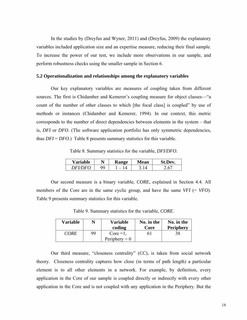
In the studies by (Dreyfus and Wyner, 2011) and (Dreyfus, 2009) the explanatory

variables included application size and an expertise measure, reducing their final sample.

To increase the power of our test, we include more observations in our sample, and

perform robustness checks using the smaller sample in Section 6.

5.2 Operationalization and relationships among the explanatory variables

Our key explanatory variables are measures of coupling taken from different

sources. The first is Chidamber and Kemerer’s coupling measure for object classes—“a

count of the number of other classes to which [the focal class] is coupled” by use of

methods or instances (Chidamber and Kemerer, 1994). In our context, this metric

corresponds to the number of direct dependencies between elements in the system – that

is, DFI or DFO. (The software application portfolio has only symmetric dependencies,

thus DFI = DFO.) Table 8 presents summary statistics for this variable.

Table 8. Summary statistics for the variable, DFI/DFO.

Variable N Range Mean St.Dev. DFI/DFO 99 1 – 14 3.14 2.67

Our second measure is a binary variable, CORE, explained in Section 4.4. All

members of the Core are in the same cyclic group, and have the same VFI (= VFO).

Table 9 presents summary statistics for this variable.

Table 9. Summary statistics for the variable, CORE.

Variable N Variable coding

No. in the Core

No. in the Periphery

CORE 99 Core =1, Periphery = 0

61 38

Our third measure, “closeness centrality” (CC), is taken from social network

theory. Closeness centrality captures how close (in terms of path length) a particular

element is to all other elements in a network. For example, by definition, every

application in the Core of our sample is coupled directly or indirectly with every other

application in the Core and is not coupled with any application in the Periphery. But the

19

number of steps (path length) needed to go from one element to another generally differs

across elements. Fewer steps imply less distance, hence greater “closeness”.

For a given element in a connected set, we can calculate the shortest distance

(number of steps) from that element to every other and sum those distances. Then, as is

conventional, we calculate closeness centrality (CC) as the reciprocal of the sum of

distances (Opsahl et al., 2010). Higher values of CC correspond to higher levels of

coupling. (Note: we multiplied the CC measures by a constant to make the coefficients

easier to interpret). Note that the distance from one element to another is finite only if

two elements are connected; thus closeness centrality is normally calculated only for the

largest connected components in a network, that is, the Core. Periphery applications are

coded as 0 (Opsahl et al., 2010). Table 10 presents summary statistics for the CC variable.

Table 10. Summary statistics for the variable, CC.

Variable N Range Mean St.Dev. CC 99 0 – 2.94 1.40 1.14

We should note that closeness centrality was used as a measure of coupling by

(Dreyfus and Wyner, 2011), and found to be positively correlated with COST. (Our

sample size is different however, thus our measures are not identical.)

In summary, for each application in the sample, the basic measure of coupling is

Chidamber-Kemerer’s measure, operationalized through DFI/DFO. The Core-Periphery

classification (CORE) adds information about indirect dependencies between components.

Finally, the closeness centrality (CC) variable adds information about the relative

closeness of those components that are located in the Core.

5.3 Correlation analysis

As a first test of H1, Table 11 shows the Pearson correlation between the

explanatory variables (DFI/DFO, CORE, and CC) and COST. All three coupling

variables are significantly correlated with COST, thus H1 is supported by this test.

20

Table 11. Pearson correlation between explanatory variables and COST.

N DFI/DFO CORE CC 99 0.502*** 0.595*** 0.613***

*** p < 0.001

5.4 Regression Analysis

Simple correlations can be misleading if the explanatory variables happen to be

correlated with omitted control variables. This problem can be addressed using multiple

regression analysis. Thus we added control variables to the test in order to estimate COST

with Ordinary Least Squares (OLS) regression. For 99 (or in one case, 98) software

applications, (Dreyfus, 2009) obtained data on five application characteristics from the

survey administered to IT Service Owners. He also recorded the respondent’s level of

experience with the application. We used these variables as controls (cf. Table 12) in a

linear regression model (cf. Table 13).

VENDOR measures if an application is developed by a vendor or in-house.

CLIENT measures if an application is accessed by end-users or not. COMP measures if

an application is focused on computation or some other task. NTIER measures if an

application has an N-tier architecture or some other type of architecture, such as client-

server or monolithic. ACTIVE measures the current development phase of an application,

if it is being actively enhanced or is currently static (e.g., maintenance mode). Finally,

APP_EXP measures the respondent’s experience with the application in question: this

variable is included as a control for possible respondent bias (e.g., Service Owners might

perceive that unfamiliar applications are harder to change, all else being equal).

Table 12. Control variables in the OLS regression model.

Name Variable coding N VENDOR Vendor =1, In-house = 0 98 CLIENT Yes = 1, No = 0 99 COMP Computation = 1, Other = 0 99 NTIER N-tier = 1, Other = 0 99

ACTIVE Active = 1, Static = 0 99 APP_EXP Less than 1 year = 1,

1 – 5 years = 2, More than 5 years =3

99

21

Table 13 shows the results of a series of regression models predicting COST using

the explanatory and control variables. One application was missing data for VENDOR,

thus our regression tests were conducted with a sample of N=98.

Note that CORE and CC are highly correlated (Correlation = .972), thus cannot be

included in the same regression without compromising the coefficient estimates. To

address this statistical problem, we regressed the original CC measures on DFI/DFO and

CORE and calculated residuals. These residuals reflect the incremental information found

in CC that is not implicit in the DFI/DFO and CORE variables. Thus our test determines

to what extent CC adds explanatory power to the other two measures.

In Table 13 all three explanatory variables are highly significant when included

individually in the regression models. Consistent with H1, the coefficients on the

coupling measures have a positive sign: higher coupling is correlated with higher change

cost (and lower architectural flexibility). F-tests strongly reject (p<.001) the null

hypothesis of no explanatory power in the regressions. The best performing single

measure of coupling, after including the set of control variables, is CORE (Model 2), with

an adjusted R2 of .52 and an f-value of 16.28 (p<.001).

Table 13. OLS results for performance variable, COST.

COST Model 1 Model 2 Model 3 Model 4 VENDOR -3.04* -3.23* -2.73* -3.67** CLIENT -1.24 -0.93 -1.00 -0.82 COMP -0.69 -0.49 -0.69 -0.51 NTIER 1.27 0.09 -0.06 0.17

ACTIVE 4.04** 4.58*** 4.13*** 4.68*** APP_EXP 1.52* 1.50** 1.46** 1.58** DFI/DFO 0.73*** 0.22

CORE 5.94*** 5.02*** CC 2.58***

CC (res) -0.86

Constant 9.51*** 8.33*** 8.52*** 8.14*** Adj. Rsquare 0.42 0.52 0.51 0.54

f 11.24*** 16.28*** 15.34*** 13.67*** Observations 98 98 98 98

* p<0.05, ** p<0.01, and ***p<0.001

22

In model 4, we include all three measures in the same regression model (using the

residuals for CC, as discussed above) and compare it to the best single-variable model

(Model 2). CORE remains highly significant (p<.001). However, coefficients on the

other two coupling measures are not significant (at the .05 level) in the presence of CORE.

We discuss these results and report robustness checks in Section 6.2 below.

6. DISCUSSION

6.1 Architecture and component classification

As presented in (Baldwin et al., 2013), the hidden structure method was originally

designed based on the empirical regularities observed across a sample of 1,287 software

codebases. That work focused on single software systems and analyzed dependencies

between source files. That is, it focused on capturing the internal coupling for each

system. In this paper we use the same method, but apply it to the dependencies between

components in an enterprise architecture. That is, we focus on external coupling, not only

between different software applications, but also between infrastructure components (e.g.,

databases and hardware) and business entities (e.g., groups). In the case described, the

method reveals a “hidden” core-periphery structure, uncovering new facts about the

architecture that could not be gained from other visualization procedures or standard

metrics. Of course, this is only one set of data from one company, hence additional

studies are needed to confirm the benefits of this method. A second study using data from

a Telecom company is presented in (Lagerström et al., 2013).

Compared to other complexity, coupling, and modularity measures, this method

considers not only the direct dependencies between components but also the indirect

dependencies. These indirect dependencies provide important input for management

decisions. For instance, it is plausible that components classified as Periphery or Control

are less costly to modify than Shared or Core components because of the lower

probability of a change spreading and affecting other components. The analysis of change

cost in Section 5 presents evidence to support this conjecture. A recent study by

(Sturtevant, 2013) of a large commercial codebase also supports the idea that indirect

dependencies are an important determinant of change cost. This information can be used

23

in change management, project planning, risk analysis, and so on.

Direct dependencies between architectural components are easily measured, while

indirect dependencies require additional processing and matrix operations. However,

looking at the direct dependencies alone can be misleading: a component can have very

few direct linkages, but many indirect ones. For example, in Table 4, components 324,

333, 347 769, and 1030 all have low Direct Fan-In (DFI) and Direct Fan-Out (DFO).

Hence, those components might be considered low risk when implementing changes. But

when we look at the Visibility Fan-In (VFI) and Visibility Fan-Out (VFO) numbers,

which capture also the indirect dependencies, we see that component 333 belongs to the

Core, while components 324, 347, and 403, are classified as Shared. The hidden structure

method therefore provides valuable information over and above that which can be

derived from direct coupling measures. Our correlation analysis (cf. Table 11) and

regression models (cf. Table 13) further support this conclusion.

It is helpful to organize a Design Structure Matrix by type of component (what we

call the “architect’s view,” cf. Figure 3). If the matrix elements are arranged in an order

that comes naturally for most companies, with the business layer at one end,

infrastructure at the opposite end, and software in between, we see that 1) the business

groups depend on the software applications, 2) software applications communicate with

each other in what looks like a clustered network of dependencies, 3) software

applications depend on the schemas and application servers, 4) the schemas depend on

database instances, and 5) the database instances depend on the database hosts. Although

these observations are neither new nor surprising, they do help validate that the

components in the investigated architecture interact as expected.

In our experience, we have found that many companies working to understand

enterprise architecture have blueprints that describe their organization, often with entity-

relationship diagrams containing boxes and arrows. Figure 5 is a typical example. When

the architecture is visualized using this type of model, however, the result is typically a

“spaghetti” tangle of components and dependencies that are difficult to interpret. This

type of representation can be translated directly into the architect’s view DSM (cf. Figure

3), which along with the entity-relationship model, can be used to trace the direct

dependencies between components. The hidden structure method can then be used to

24

rearrange the DSM, as in Figure 4, permitting the architecture to be classified, and

components grouped into Core, Shared, Control, and Periphery. Thereafter, measures

such as the size of the Core, propagation cost and the “flow through” of the architecture

can be generated, which can prove useful when trying to improve an architecture, by

assessing future actions in terms of the desired impact on these metrics.

Figure 5. Example of an enterprise architecture blueprint.

6.2 Cost analysis

Our statistical tests (cf. Table 11 and Table 13) of H1 show that being coupled (by

any measure) is correlated with higher change cost hence lower architectural flexibility.

However, they also reveal significant differences among the measures of coupling. The

simplest measure we analyze is Chidamber-Kemerer’s measure of direct coupling,

operationalized as DFI/DFO. The CORE measure goes one step further and identifies

applications with the highest level of direct and indirect coupling. Although DFI/DFO is

a scalar measure, CORE is binary because all applications in the Core of the system are

connected to each other, hence have the same VFI/VFO.

The regression of COST on CORE (Model 2) significantly outperforms the

regression of COST on DFI/DFO, with the adjusted R2 increasing from 42.2% to 52.2%.

This indicates that indirect dependencies have a significant positive impact on change

cost and a corresponding negative impact on architectural flexibility. Furthermore, when

25

CORE and DFI/DFO are included in the same regression, the coefficient on DFI/DFO is

insignificant. (This is true when only CORE and DFI/DFO are included, as well as when

all three coupling measures are included in the same model.) This result suggests that the

explanatory power of DFI/DFO in Model 1 arises because this variable is an (imperfect)

proxy for Core membership. Put another way, applications with high DFI/DFO are more

likely to be in the Core; however, within the Core itself (or the Periphery), higher levels

of direct coupling seem to have no incremental impact on the level of change cost.

Critically, we find Core membership is economically as well as statistically

significant. In particular, we can use the results of Model 2 as a predictive equation,

inputting sample means for each of the control variables. From this, we obtain a

predicted cost of 15.63 for an “average” application in the Core versus 9.69 in the

Periphery. Taking the ratio of these estimates, we find that for the “average” application,

Core membership increases the predicted change cost by approximately 60%.

Moving on, closeness centrality (CC) is a scalar coupling measure that is

mathematically related to CORE as follows:

CCi = ∗

, (4)

where CCi and COREi are the CC and CORE metrics for application i, NC is the

number of applications in the Core (=61), and ̅ is the average distance (number of steps)

between application i and the rest of the applications in the Core. In this sample, CORE

and CC are highly correlated, hence including both in the same regression model

compromises coefficient estimates.

Since CORE is a binary measure and CC is a scalar measure, CC contains more

information than CORE. The question is, does this extra information provide additional

explanatory power? The evidence here is mixed. When the residuals of CC (predicted by

CORE) are included in a regression with DFI/DFO and CORE, the adjusted R2 increases

from 51.2% to 53.8%, but the coefficient is not significant at the 5% level (cf. Models 2

and 4 in Table 13). We formally tested the hypothesis that one or both of the coefficients

of DFI/DFO and CC_res in Model 4 are greater than zero vs. the null hypothesis that

they are both zero. We are able to reject the null hypothesis at the 10% level of

significance but not at the 5% level. Thus there is a greater than 90%, but less than 95%

26

chance that the one or both of the coefficients of DFI/DFO and CC_res are non-zero.

We conclude that a modest amount of explanatory power is gained by adding data

about direct coupling and closeness centrality to the basic Core/Periphery measure of

coupling. (Note that in our final model, the coefficients on the two additional measures

have opposite signs, indicating that their effects tend to cancel).

6.3 Robbustness Checks

We performed robustness checks on the statistical tests presented in Table 13.

First, our basic specification does not control for the size or number of files in each

application, although these variables might plausibly affect change cost. Data on size

(measured as lines of code) and files was available for a subsample of 60 applications in

the dataset. We ran Models 1 – 4 on this smaller sample, including size and files as

control variables. As expected, the explanatory power of the test declined as a result of

this decrease in sample size. However, the coefficients on the coupling variables were

consistent with the results above, while the size and files controls were insignificant.

Thus omitting these controls in the larger sample did not compromise the statistical tests.

In our tests, we measured change cost (the inverse of architectural flexibility)

using estimates obtained from IT Service Owners at BioPharma. A better way to measure

change cost would be to look at the actual costs of changing the listed applications.

Unfortunately, we did not have access to such data. Given that change cost is estimated

from survey data, a legitimate concern is that IT Service Owners may estimate change

costs in different ways depending upon their experience. Indeed, Table 13 shows that

application experience (APP_EXP) is consistently positive and significant, indicating that

Service Owners with more experience in a given application were more pessimistic on

average than those with less experience. (The data did not allow us to determine whether

more experienced Service Owners were more pessimistic overall.) Thus it is reasonable

to ask whether experience differentially affects estimates of change cost for applications

in the Core versus the Periphery.

To investigate this possibility, we added a cross-product variable to Model 2. The

cross-product was equal one if the application was in the Core and the Service Owner

providing cost estimates had greater than one year’s experience and zero otherwise. If

27

experienced Service Owners systematically assessed the change cost of Core applications

higher (or lower) than inexperienced ones, then the coefficient of this interaction variable

would be significantly positive (or negative). After running this test however, we found

that the coefficient on the cross-product term was not significantly different from zero,

and the coefficients on the CORE and control variables were essentially unchanged. We

conclude that differences in respondents’ experience levels did not bias the estimates of

change cost for those software applications in the Core.

7. RESEARCH OUTLOOK

While the first step in future research should be to apply this method for revealing

hidden structure to additional enterprise architectures (see, for example, Lagerström et al.,

2013) there are a number of areas in which the method could be further developed.

In previous work by (Baldwin et al., 2013) and (Lagerström et al., 2013), as well

as in this case, the architectures studied have had a single large Core. A limitation of this

method is that it shows which elements belong to the Core, but does not help in

describing the inner structure of this Core. (In contrast, closeness centrality provides

information about the relative closeness of elements in the Core.) Thus, future research

might extend the method to help identify those elements within the Core that are most

important in terms of dependencies, component clustering and change cost. Our

hypothesis is that there are some elements in the Core that bind the group together or

span what might otehrwise be separate groups. As such, removing these elements or

reducing their dependencies (either to or from them) may decrease the size of the Core

and thus the complexity of the architecture. Identifying these elements might help

pinpoint where the Core is most sensitive to change.

While the method described is founded upon directed dependencies, we note that

software application portfolio architectures often contain non-directed dependencies, thus

forming symmetric matrices that have special properties and behave differently. This

could, for instance, be due to the nature of the dependency itself or due to imprecision in

capturing the data (e.g., because of the high costs of data collection). For a firm, the

primary concern may be whether two applications are connected, the direction of the

dependency being secondary. In one company we studied, the firm had more than a

28

thousand software applications but no application portfolio description, much less an

architectural model of its system. For this firm, collecting information about the

applications it had and what each one did was of primary importance. That process was

costly, and consequently the direction of the dependencies between the applications was

not considered a priority. Exploring how our method applies to symmetric dependency

networks, being a special case of an enterprise architecture, might be useful to investigate.

More effective tools would lower the high costs associated with data collection

for enterprise architectures. In prior work by (Baldwin et al., 2013), the analysis of

internal coupling was supported by tools that extracted the source files and created a

dependency graph automatically from software code. In the software portfolio domain,

such tools generally do not yet exist. Consequently, data collection requires considerable

time and effort. The most common methods of establishing dependencies and change

costs are interviews and surveys of people (often managers) with already busy schedules.

As such, future work must be directed towards data collection in the software portfolio

and enterprise architecture domains. While some work has been done, it is limited in

either scope or application, as noted in (Holm et al., 2012) and (Buschle et al., 2012).

Indeed, at a broader level, for this method to be most useful for practice, it needs

to be incorporated into existing or future architecture modeling tools. Most companies

today already use modeling software like Rational System Architect (IBM, 2013),

BiZZdesign Architect (BiZZdesign, 2013), TrouxView (Troux solutions, 2013), ARIS 9

(Software AG, 2013), and MooD Business Architect (MooD International, 2013) to

describe their architecture. Thus, having a stand-alone tool that supports this method is

not cost efficient. Moreover, if the method could be integrated into current tools,

companies could perform this analysis by re-using existing architecture descriptions.1

Last, but not least, the most important future work will be to test the VFI/VFO

metrics and the classification of elements (as Shared, Core, Periphery, and Core) with a

greater number of performance metrics and with data from other cases and industries.

1 The modeling software Enterprise Architecture Analysis Tool (EAAT) (Industrial Information and

Control Systems, 2013) (Buschle et al., 2011) is currently implementing this method.

29

8. CONCLUSION

Our results suggest that the hidden structure method can reveal new facts about an

enterprise architecture and aid the analysis of change costs at the software application

portfolio level. Our analysis reveals that the structure of the enterprise architecture at

BioPharma can be classified as core-periphery with a propagation cost of 23% and a Core

size of 32%. Our statistical tests show that the software applications in the Core are

associated with a greater cost to change (i.e., less architectural flexibility) than those in

the Periphery. Furthermore, we find that this relatively simple metric outperforms other

measures of coupling used in the prior literature, in terms of predicting change cost.

For BioPharma, this method for architectural visualization and the associated

coupling metrics could provide valuable input when planning architectural change

projects (in terms of, for example, risk analysis and resource planning). In future work,

we plan to gather more evidence supporting the usefulness of this method, both by

applying it to more software application portfolio architectures and by testing the

resulting measures of architecture classification and component coupling against

performance outcome metrics of interest to firms.

30

REFERENCES

Alexander, C. 1964. Notes on the Synthesis of Form. Harvard University Press.

Baldwin, C. and Clark, K. 2000. Design Rules, Volume 1: The Power of Modularity. MIT Press.

Baldwin, C., MacCormack, A., and Rusnack, J. 2013. Hidden structure: Using network methods to map

system architecture. Harvard Business School Working Paper 13, 093.

Barabási, A. 2009. Scale-free networks: A decade and beyond. Science 325, 5939, 412-413.

BiZZdesign, BiZZdesign Architect, www.bizzdesign.com/tools/bizzdesign-architect, accessed May 2013.

Brown, N., Cai, T., Guo, Y., Kazman, R., Kim, M., Kruchten, P., Lim, E., Nord, R., Ozkaya, I., Sangwan,

R., Seaman, C., Sullivan, K., and Zazworka N. 2010. Managing technical debt in software-reliant

systems. In Proceedings of the FSE/SDP Workshop on the Future of Software Engineering Research

(FoSeR'10), 47-52.

Buschle, M., Grunow, S., Matthes, F., Ekstedt, M., Hauder, M., and Roth, S. 2012. Automating enterprise

architecture documentation using an enterprise service bus. In Proceedings of the 18th Americas

Conference on Information Systems (AMCIS). Association for Information Systems.

Buschle, M., Ullberg, J., Franke, U., Lagerström, R., and Sommestad, T. 2011. A tool for enterprise

architecture analysis using the PRM formalism. Information Systems Evolution, 108-121.

Chidamber, S. R., and Kemerer, C. F. 1994. A metrics suite for object oriented design. IEEE Transactions

on Software Engineering 20, 6, 476-493.

Dreyfus, D. 2009. Digital Cement: Information System Architecture, Complexity, and Flexibility. PhD

Thesis. Boston University Boston, MA, USA, ISBN: 978-1-109-15107-7.

Dreyfus D. and Wyner, G. 2011. Digital cement: Software portfolio architecture, complexity, and

flexibility. In Proceedings of the Americas Conference on Information Systems (AMCIS),

Association for Information Systems.

Eppinger, S. D., Whitney, D.E., Smith, R.P., and Gebala, D. A. 1994. A model-based method for

organizing tasks in product development. Research in Engineering Design 6, 1, 1-13.

Fenton, N. and Melton, A. 1990. Deriving structurally based software measures. Journal of Systems and

Software 12, 3, 177-187.

31

Hall, N. R., and Preiser, S. 1984. Combined network complexity measures. IBM journal of research and

development 28, 1, 15-27.

Halstead, M. 1977. Elements of software science. Operating and Programming Systems Series. Elsevier

Science Inc.

Henry, S. and Kafura, D. 1981. Software structure metrics based on information flow. IEEE Transactions

on Software Engineering 7, 5, 510-518.

Hinsman C., Snagal, N., and Stafford, J. 2009. Achieving agility through architectural visibility.

Architectures for Adaptive Software Systems, LNCS 5581, 116-129.

Holm, H., Buschle, M., Lagerström, R., and Ekstedt, M. 2012. Automatic data collection for enterprise

architecture models. Software & Systems Modeling. Online first.

IBM, Rational System Architect, www.ibm.com/software/products/us/en/ratisystarch, accessed May 2013.

IEEE Standards Board 1990. IEEE Standard Glossary of Software Engineering Technology. Technical

report. The Institute of Electrical and Electronics Engineers.

Industrial Information and Control Systems - the Royal Institute of Technology, The Enterprise

Architecture Analysis Tool (EAAT), www.ics.kth.se/eaat, accessed May 2013.

Jenkins, S. and Kirk, S. 2007. Software architecture graphs as complex networks: A novel partitioning

scheme to measure stability and evolution. Information Sciences 177, 12, 2587-2601.

Lagerström, R., Baldwin, C., MacCormack, A., and Aier, S. 2014. Visualizing and Measuring Enterprise

Application Architecture: An Exploratory Telecom Case. In Proceedings of the Hawaii

International Conference on System Sciences (HICSS-47), IEEE.

Laird, L. and Brennan, M. 2006. Software Measurement and Estimation: A Practical Approach. Wiley-

IEEE Computer Society Pr.

LaMantia, M., Cai, Y., MacCormack, A., and Rusnak, J. 2008. Analyzing the evolution of large-scale

software systems using design structure matrices and design rule theory: Two exploratory cases. In

Proceedings of the 7th Working IEEE/IFIP Conference on Software Architectures (WICSA7).

MacCormack, A., Baldwin, C., and Rusnak, J. 2006. Exploring the duality between product and

organizational architectures: A test of the "mirroring" hypothesis. Research Policy 41, 8, 1309-1324.

McCabe, T. 1976. A complexity measure. IEEE Transactions on Software Engineering 2, 4, 308-320.

32

Mead, C. and Conway, L. 1980. Introduction to VLSI Systems. Addison-Wesley Publishing Co.

MooD International, MooD Business Architect, www.moodinternational.com/moodplatform, accessed May

2013.

Myers, C. R. 2003. Software systems as complex networks: Structure, function, and evolvability of

software collaboration graphs. Physical Review E 68, 4, 046116.

Opsahl, T., Agneessens, F., and Skvoretz, J. 2010. Node centrality in weighted networks: Generalizing

degree and shortest paths. Social Networks 32, 3, 245-251.

Ozkaya, I. 2012. Developing an architecture-focused measurement framework for managing technical debt.

In Software Engineering Institute blog. http://blog.sei.cmu.edu/post.cfm/developing-an-architecture-

focused-measurement-framework-for-managing-technical-debt, accessed Sept. 2013.

Parnas, D. L. 1972. On the criteria to be used in decomposing systems into modules. Communications of

the ACM 15, 12, 1053-1058.

Simon, H. A. 1962. The architecture of complexity. American Philosophical Society 106, 6, 467-482.

Software AG, ARIS 9, www.softwareag.com/corporate/products/aris_platform, accessed May 2013.

Sosa, M., Eppinger, S., and Rowles, C. 2007. A network approach to define modularity of components in

complex products. Transactions of the ASME 129, 1118-1129.

Stevens, W. P., Myers, G. J., and Constantine, L. L. 1974. Structured design. IBM Systems Journal 13, 2,

115-139.

Steward, D. 1981. The design structure system: A method for managing the design of complex systems.

IEEE Transactions on Engineering Management 3, 71-74.

Sturtevant, D. J. 2013. System design and the cost of architectural complexity. Diss. Massachusetts

Institute of Technology.

Troux solutions, TrouxView™ Enterprise Portfolio Management, www.troux.com, accessed May 2013.

Wilkie, F. G., and Kitchenham, B. A. 2000. Coupling measures and change ripples in C++ application

software. Journal of Systems and Software 52,2, 157-164.