visualization with paraview on stampede · visualization with paraview on stampede ben trumbore...

Visualization with ParaView

on Stampede

Ben Trumbore

Computational Scientist

Cornell University Center for Advanced Computing (CAC)

[email protected]

High Performance Computing on Stampede 2, with KNL

January 23, 2017

www.cac.cornell.edu

mailto:[email protected]

Preparation for Lab

1/23/2017 www.cac.cornell.edu 2

Get ParaView onto the lab PC

• Download “ParaView.zip” using link in workshop agenda

• Double-click downloaded file and select “ParaView-5.2.0” folder

• Extract folder to desktop or “Downloads” folder

Alternatively, download and install (esp. Mac, Linux users)

• http://www.paraview.org/download/

• Windows note: get version without “MPI” for workshop.

• MPI version of ParaView requires also installing Windows MPI

Get data files onto the computer that will run ParaView

• Download http://cvw.cac.cornell.edu/ParaView/data.zip

• Double-click downloaded file and select “data” folder

• Extract folder to some location on the computer

http://www.paraview.org/download/



https://www.microsoft.com/en-us/download/details.aspx?id=54607

http://cvw.cac.cornell.edu/ParaView/data.zip

Visualization


Benefits of visualizing scientific data

• Easier to analyze complex data sets

• Convey meaning in publications via images

• Visualize a fourth dimension using animations

Visualization on Stampede


Software available on Stampede

• Ncview – netCDF data

• ParaView

• Visit

• VMD – Molecular Dynamics

Advantages of visualizing on Stampede

• Many processors can be used

• Large memory for large data sets

• Environment modules constructed appropriately for Stampede and Stampede 2

http://meteora.ucsd.edu/~pierce/ncview_home_page.html

https://www.google.com/url?sa=t&rct=j&q=&esrc=s&source=web&cd=1&cad=rja&uact=8&ved=0ahUKEwiJrvHHrqnRAhWFNiYKHZb_DlwQFggaMAA&url=http://www.paraview.org/&usg=AFQjCNFSh07NI7sHd8inypOR-hA6HG8_KA&sig2=9vSn7WqXDrjLH_p4g5_GgA&bvm=bv.142059868,d.eWE

https://wci.llnl.gov/simulation/computer-codes/visit

https://www-s.ks.uiuc.edu/Research/vmd/

ParaView


ParaView Features

• Free (sponsored by Kitware, Sandia National Laboratory, Los Alamos

National Laboratory, Army Research Laboratory)

• Mature open-source software

• Feature rich, general purpose

• Can run it on your workstation and on Stampede

• Handles many types of input data

• Extensible through plugins and scripting

• Built to take advantage of parallelism

• No longer requires great graphics hardware

• Can generate and export animations

Goals for this Presentation


Explore Major ParaView Functionality

• User interface

• Common work flows

• Popular data types, filters

• Animations

• Tips and tricks

Introduce other functionality

• Scripting

• Ray Traced rendering

• In situ visualizations, integrated with simulations

Bonus coverage: Using the Stampede Visualization Portal

The Visualization Pipeline


ParaView’s Visualization Pipeline consists of trees of source and filter nodes

• Sources bring data into ParaView

• Filters transform the output of other nodes into new data

• Multiple filters can be connected to a source or filter node

• Multiple “Views” can independently set visibility for each node

CAT

scan Slice

Regular grid

Contour

Crop

Slice

Plot Over Line

2D grid

Triangles

Smaller 2D grid

Lines in plane

2D graph

User Interface


Steps:

• Run bin\paraview.exe

Three main UI components

1. Pipeline Browser

2. Properties and Information

3. Views

Commands available via

• Menus

• Toolbars

• Context menus

• Hot keys

Some toolbars hidden for clarity

Instructions all use menus

Pipeline Browser


“builtin” is the current server

Steps to add a source

• Sources->Cylinder

• Click “Apply” in Properties

• Eye symbol controls visibility

• Left click to rename node

• Right click for context menu

• Delete

• Change Input (re-parent)

Information Panel


Click “Information” Tab (1)

Displays read-only data about node

• For node selected in browser

• Output data type

• Data arrays at samples (2)

• Bounds (3)

Properties Panel


Click “Properties” tab (1)

Shows user-editable node properties

• For node selected in browser

• Three sections

• Properties (node options)

• Display (geometry) (2)

• View (rendering)

• Steps

• Change cylinder resolution (3)

• Click Apply after changes (4)

• “Gear” to toggle Advanced options

Display and View Properties


Control rendering of node

• Expandable sections (1)

• Changes are immediate

• Steps

• Representation =

Surface with Edges (2)

• Coloring = TCoords (3)

• View properties include

• Axes visibilities

• Background color

Render Views


Views of pipeline nodes

• Create additional tabs (1)

• Must specify view type

• Subdivide view panes (2)

• Must specify view type

• Selected pane has blue outline

• Node visibility is per view

• Camera has undo stack (3)

To see/change view controls

• Edit->Settings, Camera tab

• Uses all three mouse buttons

• Uses shift & control modifiers

Saving and Loading


Saving your work

• File->Save State saves the current pipeline and all property settings

• File->Load State loads a previously saved pipeline

• State files include absolute references to data sources. Not portable!

Exporting data and results

• File->Save Data exports selected node as CSV polygons/points

• File->Save Screenshot… saves image of selected View

Saving the user interface layout

• File->Save Window Layout saves current visibility/size for all panels

• File->Load Window Layout loads a saved panel layout

Data Types


Images from The Visualization Toolkit by Schroeder et al.

Unstructured Points Unstructured Grid (Finite element analysis)

Structured Grid (Engineering Model)

Regular Grid (Medical scan, Image)

Rectilinear Grid

(fluid dynamics)

Polygonal Data (CAD model)

Data File Formats


ParaView can import data in more than 70 file formats.

Formats included at installation include

• CSV

• Raw Binary

• VTK

• PVD

Plugins at installation can import these formats and more

• AnalyzeNifti

• GMV

• HDF5 Particle

http://paraview.org/Wiki/ParaView/Users_Guide/List_of_readers

Additional Data at Sample Points


Data sets can contain additional information that is useful for visualizations

• Scalars (density, temperature, pressure)

• Vectors (velocity, momentum)

• Normals (perpendicular to surface, for shading)

• Texture Coordinates (map between model space and texture space)

• Tensors (generalization of scalars and vectors)

Sample Problem


Want to visualize data set, a medical scan of a head

We want to create iso-surfaces for the skin and bone

• An iso-surface is a set of triangles through sample points with the same

scalar value, in this case “density”

How do we find the densities of those features?

• We first need to look at some statistics for the data

• Do this by creating a cross section “slice” and studying its density values

Loading a Data Source


Steps

• Edit->Reset Session to clean up

• File->Open “headsq.vti”

• Could also drag-drop the file

• Notice that node is not yet visible

• “Apply” to initialize properties

• Notice that bounding box is shown

• In Display section

• Representations = “Slice”

• Representations = “Outline”

Slice View


Before adding a Slice filter to the pipeline, explore slice locations

Steps

• Split Render View horizontally

• Type of new view is “Slice”

• Make Source node visible in view

• Rotate view to see slices in 3D

• Margin guides change slices

• Drag to reposition a slice

• Right click to hide a slice

• Double-click to add/remove

• Drag Z guide for best cross section

• Can see skull best around 20

• Close Slice View pane

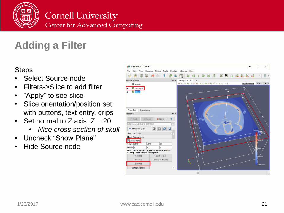
Adding a Filter


Steps

• Select Source node

• Filters->Slice to add filter

• “Apply” to see slice

• Slice orientation/position set

with buttons, text entry, grips

• Set normal to Z axis, Z = 20

• Nice cross section of skull

• Uncheck “Show Plane”

• Hide Source node

Statistics Filters - Histogram


Statistics filters and views allow us to learn about the data

Steps for Histogram

• Select Slice node

• Filters->Histogram to add filter

• “Apply”, get new “Bar Chart” view

• Change Bin Count to 30, “Apply”

• Right click Histogram node

• Change Input…


• Note histogram is similar

Statistics Filters – Plot Over Line


Steps

• Select Slice node

• Filters->Plot Over Line

• “Apply”, get new “Line Chart” view

• Select Render view to see line

• Set Y of Points to 60

• “Apply” to update plot over line

• Likely skin densities around 600

• Likely bone densities around 1200

• Right click on Line Chart view title

• Convert To: Spreadsheet

• Close two statistics views

Steps

• Edit->Reset Session

• File->Open “headsq.vti”, “Apply”

• Filters->Contour to create Contour

• Filter creates triangles, normals

• Check “Compute Scalars”, “Apply”

• Contouring requires scalars


• In Properties – Isosurfaces

• Value at index 1 = 1200, “Apply”

• Surface for bone and teeth

• “+” adds index, value = 600, “Apply”

• Surface for skin, other content

Creating an Iso-surface


Color Maps


About color maps

• A color map is associated with each of a Source’s data arrays

• We are seeing the default color map for the “Scalars_” array

• Can be loaded, edited and saved and can also map opacities

• Maps commonly specify value ramps, but can also be look-up tables

Coloring the Iso-Surface


Steps to edit a color map

1. In Display – Coloring:

• Select data array

• Click “Edit”

Steps for the iso-surface

2. Check “Enable opacity

mapping for surfaces”

3. “Rescale to data range”

4. Drag opacity control at 600

up to 0.5 to see “skin”

Coloring the Iso-surface (continued)


Steps continued

1. Double click color control at

scalar value 600

• Select a pink color

2. Select color control at scalar

value 900

• Delete key to remove it

3. Double click color control at

scalar value 1200

• Select a white color

• Single click creates a control

• Can edit mapping value of a

selected interior control

More About Color Maps


“Interpret Values As Categories” (1) creates a look-up table

“Render Views” (2) toggles automatic updating

Can load and save “preset” color maps (3)

Steps

• Close Color Map Editor

Animations


Animations can be recorded from

screen or saved as OGV file

Can animate

• Camera position

• Orbit, along path, along data

• Pipeline node parameters

• Data with time-varying properties

Steps

• View->Animation View to show

UI for constructing an animation

• View->Toolbars->VCR Controls

for toolbar to play animations

Animating an Orbiting Camera


Steps

• Select node of interest.

• Camera looks at node center

• Navigate camera to initial view.

• Concern here is zoom level

• In Animation View’s last row

• Select Camera and “Orbit”

• Click “+”

• check “Center” values, click OK

• Press Play button of VCR Controls

• Leaving “Mode” as “Sequence”

• Change “No. Frames” and play

• Change Mode to “Real Time” and play

Animating a Filter Parameter


Steps to prepare data


• File->Open “headsq.vti”, “Apply”

• Filters->Slice

• Uncheck “Show Plane”

• Click “Z Normal”, “Apply”

Steps in Animation View

• Select “Slice1”, “Slice Offset Values”

• Click “+” to create new row

• Double-click row’s time bar

• In Dialog

• Time 0 Value = 92

• Time 1 Value = -92, click “OK”

• Mode = “Real Time”

• Play animation

Visualizations with Annotations


3D annotations are useful for displaying vector information

Common examples are

• Glyphs at each sample point that follow a vector direction

• Streamlines that connect multiple sample points to show continuity

Steps for next lab work

• Close Animation panel


• File->Open “RectGrid2.vtk”

• “Apply”

• Display – Representation = Points

Glyphs


Glyphs are 3D shapes displayed at some sample locations

Arrow and line glyphs are used to visualize vector data

Steps


• Filters->Glyph to add filter

• “Apply” for default glyphs


Can control glyph

• Shape and proportions

• Scaling

• Density

• Coloring

Streamlines


Streamlines can be displayed when vector field is integrated

“Stream Tracer” filter both performs integration and generates lines

Steps

• Hide Glyph node


• Filters->StreamTracer

• “Apply”

Can control

• Integration type and parameters

• Seed type and parameters

• Max number of streamlines

• Coloring

Streamlines - Seeding


Steps for larger seed

• Sphere Parameters – Radius = 0.5

• Number of Points = 200

• Uncheck “Show Sphere”

• “Apply”

Steps for line seed

• Seed Type = “Line Source”

• Point1 = -1, 0, 0.5

• Point2 = 1, 0, 0.5

• “Apply”

Streamlines


Steps for displaying tubes

• Select StreamTracer node

• Filters->Tube

• “Apply”

Steps for displaying glyphs

• Hide Tube1, select StreamTracer

• Filters->Glyph

• Vectors = “vectors”, Max = 1000

• “Apply”

OSPRay Ray Tracer


OSPRay ray tracer (http://www.ospray.org/) is integrated into ParaView

Can produce shadows, better transparency and specular highlights

Takes advantage of KNL processors in Stampede 2

Steps

• Hide all nodes except Glyph1

• Sources->Box

• X & Y Lengths = 10

• Center Z = -1

• “Apply”

• In View section

• Check Enable OSPRay

• Check Shadows

http://www.ospray.org/


Extensibility - Plugins


ParaView can be extended using Plugins

• Tools->Manage Plugins… for Plugin Manager

• Add plugins to library from binary files

• “Load” known plugins for use in current session

• Users can write their own C++ plugins for various purposes

• Filters

• Data readers and writers

• Toolbars and menus

Extensibility – Python Scripts


Users can write Python scripts to customize ParaView

Programmable Source and Programmable Filter

• In Properties, select output data type and enter Python script

• Scripts must call the “paraview” Python package

• “The ParaView Guide” contains examples that call the API

Python View

• In Properties - View, enter Python script

• Scripts must call the “paraview” Python package

• The ParaView Guide” contains examples that call the API

Python Annotation and Python Calculator Filters

• Enter Python expressions and set an array association

• Can easily call NumPy and SciPy functions and access data

http://www.paraview.org/ParaView3/Doc/Nightly/www/py-doc/






Catalyst – In Situ Visualization


Catalyst allows data to be piped from simulation process to ParaView

• Simulation code must call Catalyst API to broadcast data

• ParaView user can connect to such a process to receive the data

• Saves time to write data to disk and read it back in

• Allows data to be updated as simulation continues

• Simulation can be steered based on visualization results

• More information at http://www.paraview.org/in-situ/

http://www.paraview.org/in-situ/




Tips and Tricks


• If filters are unexpectedly disabled or unwanted grips are shown in view

• Check which pipeline node is selected

• If visualization seems wrong for recent changes

• Check if any “Apply” buttons are enabled

• Enable “auto-apply” in main toolbar

• If visualization seems really messed up

• Double-check pipeline node parenting

• If you can’t find a setting that seems like it should be there

• Enable "Advanced" properties for the node

Resources


Links

• ParaView: Home page, Download, Guide, Wiki

• TACC: ParaView on Stampede

• OSPRay

• Catalyst: Home page, User’s Guide, Wiki

Tutorials

• ParaView

• CAC Virtual Workshop

• Sandia National Labs

• Boston University Information Sciences & Technology

• For Earth and Climate Science Data

http://www.paraview.org/


http://www.paraview.org/paraview-guide/

http://www.paraview.org/Wiki/ParaView

https://portal.tacc.utexas.edu/user-guides/stampede;jsessionid=F56D81A44005D39CA3C8C23B3660CF33.node0#vis-apps-paraview



http://www.paraview.org/files/catalyst/docs/ParaViewCatalystUsersGuide_v2.pdf

http://www.paraview.org/Wiki/ParaView/Catalyst/Overview

http://www.paraview.org/Wiki/The_ParaView_Tutorial

https://cvw.cac.cornell.edu/ParaView

https://cvw.cac.cornell.edu/ParaView

http://www.paraview.org/Wiki/SNL_ParaView_Tutorials

https://www.bu.edu/tech/support/research/training-consulting/online-tutorials/paraview/

http://mms.dkrz.de/pdf/vis/paraview.pdf

ParaView on Stampede - Login


Easiest way to run ParaView on Stampede is through their Visualization Portal

• https://vis.tacc.utexas.edu

• Log in with XSEDE or TACC credentials

• Get a Linux desktop with visualization software

• Uses VNC to view desktop in web browser

https://vis.tacc.utexas.edu/

ParaView on Stampede - Request


Not yet available on Stampede 2!

After logging in

1. Make sure you are on “Jobs” tab

2. Select “Stampede” cluster

3. See if nodes are available

4. Session type is VNC

5. Queue is “vis”

6. Set number of nodes and “wayness”

7. Set a VNC password

• Do not use your login password!

• Only need to do once per account

• Others can use to view session

8. Start job

ParaView on Stampede - Starting


Dialogs will display while job is starting

Can cancel request here

If insufficient nodes, start up may fail

If success, VNC page is shown

“Desktop” tab appears. Supply VNC password

Switching tabs requires password again

Can break out a separate window

Disconnect and reconnect from here

ParaView on Stampede - Desktop


Note: Closing the default terminal ends your session

Load ParaView and its dependencies: • module load python qt/4.8.4 paraview

• “qt” version needed temporarily

Run ParaView: • vglrun paraview

• Vglrun allows GL apps over VNC

ParaView on Stampede – Add Server


Note that ParaView is initially connected to the built-in server

Steps to connect to the allocated nodes

• File->Connect

• “Add Server” in dialog

• Name server configuration, “Configure”

ParaView on Stampede – Connect to Server


Steps to connect - continued

• Startup Type = “Command”

• Enter text for external command (cannot paste via VNC): env NO_HOSTSORT=1 ibrun tacc_xrun pvserver

• “Save” to complete configuration

• “Save Servers” to save configuration for reuse via “Load Servers”

• “Connect”

ParaView on Stampede – Connected!


Dialog displays attempt to connect to server

When you see that the server is accepting connections, “Close” dialog

Pipeline Browser now shows your connection to a server running locally

ParaView on Stampede – Connected


Steps to test the parallel ParaView

• Sources->Sphere

• “Theta Resolution” = 32

• “Phi Resolution” = 32

• Representation = “Surface With

Edges”

• Coloring = “vtkProcessId”

• “Apply”

• Sphere is colored per processor

Steps to exit

• Close ParaView

• “exit” in terminal

• Disconnect in browser

visualization with paraview on stampede · visualization with paraview on stampede ben trumbore...

Documents