visualization on biohpc€¦ · - scientific visualization - work flow for visualization and...
TRANSCRIPT

Visualization on BioHPC
1
[web] portal.biohpc.swmed.edu
[email] [email protected]
Updated for 2015-09-16

Outline
2
• What is Visualization- Scientific Visualization- Work flow for Visualization and Analysis of 3D Microscopic Images
• Visualization on High Performance Computer- Storage and management of image
BioHPC OMERO (Open Microscopy Environment Remote Objects)
- 3D volume renderingConcepts and examples of different type of volume renderingGPU renderingImageJ 3D viewer plugin, Amira, Imaris, ParaviewRemote and parallel visualization
- Image processing with HPCexamples

What is Visualization
3
Visualizationa high bandwidth connection between data on a computer and a human brain.
Visualization and Analysis of 3D Microscopic Imageslarger datasets demand not just visualization, but advanced visualization resources and techniques.

Scientific Visualization : from single image/view to multiple datasets
4
raw image produced by light-sheet microscopes
Finding collagen fibers
Fiber Alignment
* Example provided by Meghan Driscoll

Scientific Visualization : from multiple datasets to a single image/view
5
Red blood cell
https://www.alcf.anl.gov/user-guides/vis-paraview-red-blood-cell-tutorial
unstructured mesh
streamline (velocity)xy-plane slice (based on velocity)
diseased cell
healthy cellparticles
Shneiderman's Mantra
6
Mantra
• overview• zoom and filter• details-on-demand
Ben ShneidermanThe Trill of Discovery: Information visualization for high-dimensional spaces
Invited talk@ center for HCI Design, City University London
September, 2007
Get Data/Images Data Storage Pre-processing Visualization Segmentation/Analysis
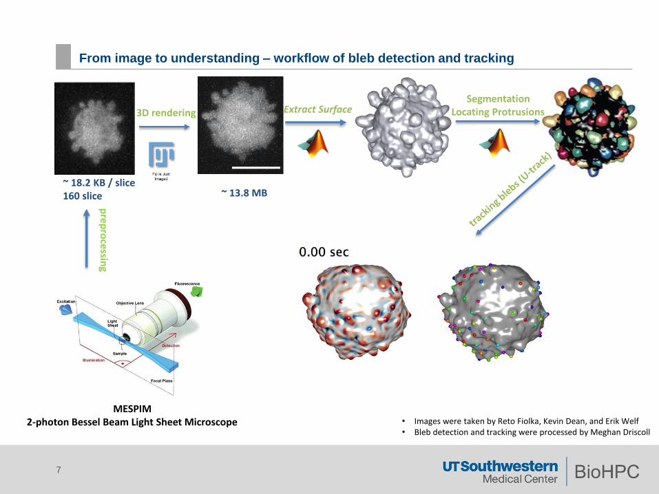
From image to understanding – workflow of bleb detection and tracking
7
~ 18.2 KB / slice160 slice
Extract Surface3D rendering
prep
rocessin
g
MESPIM2-photon Bessel Beam Light Sheet Microscope
~ 13.8 MB
SegmentationLocating Protrusions
• Images were taken by Reto Fiolka, Kevin Dean, and Erik Welf• Bleb detection and tracking were processed by Meghan Driscoll
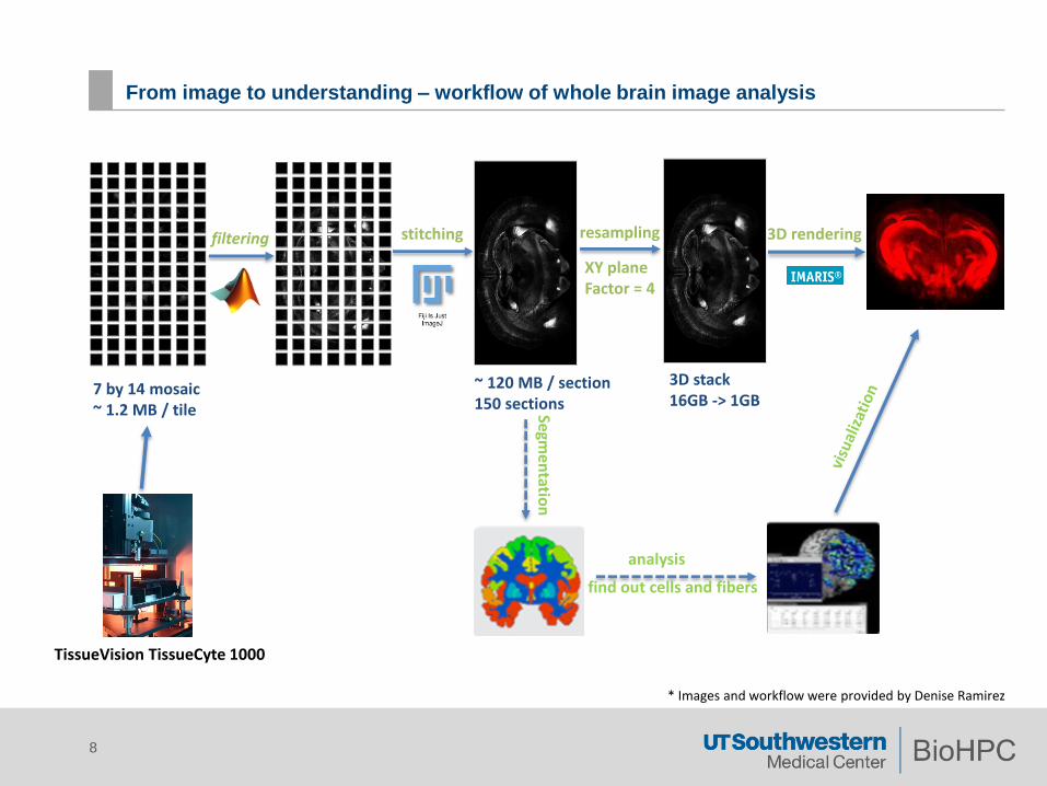
From image to understanding – workflow of whole brain image analysis
8
TissueVision TissueCyte 1000
7 by 14 mosaic~ 1.2 MB / tile
filtering stitching 3D renderingresampling
XY planeFactor = 4
~ 120 MB / section 150 sections
3D stack16GB -> 1GB
Segmen
tation
analysis
find out cells and fibers
* Images and workflow were provided by Denise Ramirez

Visualization on High Performance Computer
9
• Storage and management of image
• Volume rendering of 3D image
• Image processing with HPCmore tools :
G’MIK
Storage and management of image
10
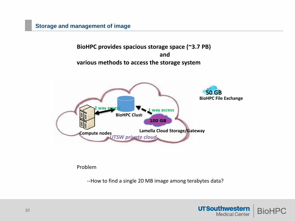
BioHPC provides spacious storage space (~3.7 PB) and
various methods to access the storage system
Problem
--How to find a single 20 MB image among terabytes data?
50 GBBioHPC File Exchange
BioHPC Cluster
Compute nodes Lamella Cloud Storage/Gateway
UTSW private cloud
1 way access2 way access

BioHPC OMERO (Open Microscopy Environment Remote Objects)
11
BioHPC OMERO Sever:http://imagebank.biohpc.swmed.edu
Client
• Download and install the OMERO desktop client from login page
• Use OMERO client module on BioHPC clustermodule add omero/5.1.0OMEROinsight_unix.sh
a modern client-server software platform for visualizing, managing, and annotating scientific image data.

Benefits of using BioHPC OMERO
12
• Keep your images well organized.• Allow you import and archive your images, annotate and tag them.• Allows you to collaborate with colleagues by creating user groups with different permission levels. • Consists of a web application and cross-platform clients, as well as ImageJ plugin, MATLAB bindings and etc.• Use OMERO as a backup of important/expensive images.

13
Use OMERO with ImageJ

Use OMERO with Matlab : open image & add comments
14
% create a connection to OMERO[session, client] = connectToBioHPCOmero;
% read image by imageIDimageId = 3117;targetImage = getImages(session,imageId);binaryData = getPlane(session,targetImage, 0, 0, 0); % z=1, time=1, channel=1
% plotfigure;imshow(binaryData);
% write commentscomments = 'comment by MATLAB';newCommentAnnotation = writeCommentAnnotation(session,comments);link1 = linkAnnotation(session, newCommentAnnotation, 'image', imageId);
% close connection to OMEROunloadOmero();
Volume rendering of 3D image
15
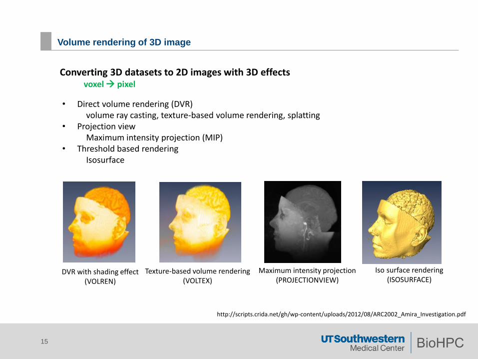
Converting 3D datasets to 2D images with 3D effectsvoxel pixel
• Direct volume rendering (DVR) volume ray casting, texture-based volume rendering, splatting
• Projection viewMaximum intensity projection (MIP)
• Threshold based renderingIsosurface
http://scripts.crida.net/gh/wp-content/uploads/2012/08/ARC2002_Amira_Investigation.pdf
Texture-based volume rendering(VOLTEX)
Maximum intensity projection(PROJECTIONVIEW)
Iso surface rendering(ISOSURFACE)
DVR with shading effect(VOLREN)
Volume rendering of 3D image
16
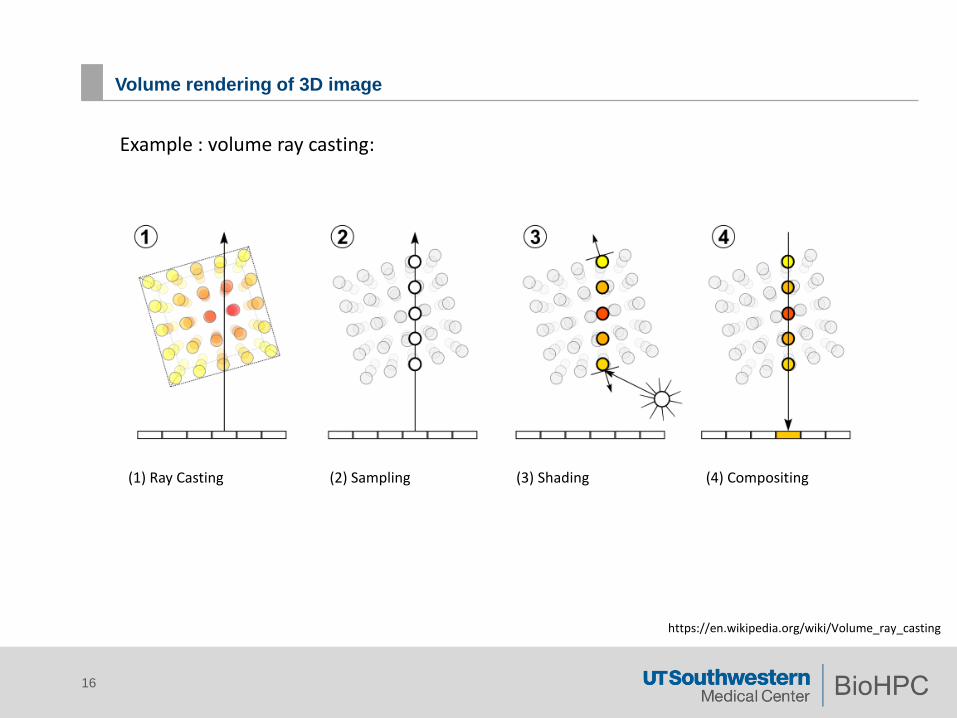
Example : volume ray casting:
(1) Ray Casting (2) Sampling (3) Shading (4) Compositing
https://en.wikipedia.org/wiki/Volume_ray_casting

How much faster is GPU rendering as compared to CPU rendering?
17
Nucleus044-049 Nucleus042-043 BioHPC Workstation
GPU card Tesla K40 Tesla K20 Quadro K600
GPU Memory 12 GB 5 GB 1 GB
GPU Memory Bandwidth 288 GB/s 208 GB/s 29.0 GB/s
CUDA cores 2880 2496 192
Benchmarking (with the same image quality)
BioHPC GPU resources
http://blog.boxxtech.com/2014/10/02/gpu-rendering-vs-cpu-rendering-a-method-to-compare-render-times-with-empirical-benchmarks/
Could be significant faster if rendering with high-end GPU : the GPU was 6.2 times faster than the CPU in this case.

BioHPC webGPU : launch a graphic environment on the Nucleus cluster
18
Web based visualization access: https://portal.biohpc.swmed.edu/terminal/webgui/
• WebGUIreserve a CPU node
• WebGPUreserve a GPU node, good for ImageJ, Amira, stand-alone paraview or compile your CUDA codestep 1: add visualization software as a modulestep 2: vglrun <software name>
• WebWinDCVreserve a GPU node, windows OS, good for Imaris
• PVGPUreserve a GPU node, client-server mode for Paraview

BioHPC WebGPU : ImageJ 3D Viewer
19
Limitations:• Can only rendering 8-bit or RGB image stack• Have to specify resampling factor, opacity
and etc. to get optimized view.• Can not rescale after resampling
• 3D visualization• Segmentation• Expandable with macros and plugins• Open-source
Maximum intensity projection

BioPHC WebGPU : Amira
20
Limitations:• Automatically resampling for large 3D tiff
stack may not give expected result when the image scale along the x, y, z direction is different.
• Requires license and we are trying to get fully support now.
• 3D visualization• Analysis and modeling system• Programmable (MATLAB)• Comprehensively equipped based package• Can be customized by adding functional extensions

BioHPC winDCV : Imaris
21
Limitations:• Only has Windows version. Can not use it on
BioHPC workstation, at present, the only way to access Imaris is via webWinDCV.
• Requires license
• 3D visualization• Analysis• Different possibilities for object segmentation• Easy to use software for quick results
BioHPC webGPU/PVGPU : Paraview
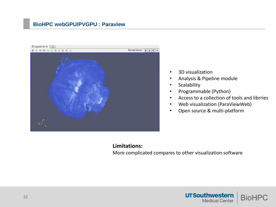
22
Limitations:More complicated compares to other visualization software
• 3D visualization• Analysis & Pipeline module• Scalability• Programmable (Python)• Access to a collection of tools and librries• Web visualization (ParaViewWeb)• Open source & multi-platform

Big Data Visualization
23
How to interactively manage visually overwhelming amounts of data
Option A: Resampling on original dataset
Option B: Parallel visualizatione.g, paraview for Interactive Remote Parallel Visualization
- Allocate multiple nodes for visualization, each node/process will process one part of the image
Original Data Subsample Rate: 2 pixels Subsample Rate: 4 pixels Subsample Rate: 8 pixels

Client-Server mode of Paraview (remote visulization)
24
ClientData
ServerRenderServer
Minimize Communication
Render Remotely
Send Images
The ParaView Guide, p. 191
Paraview with multiple processes (parallel visualization)
25
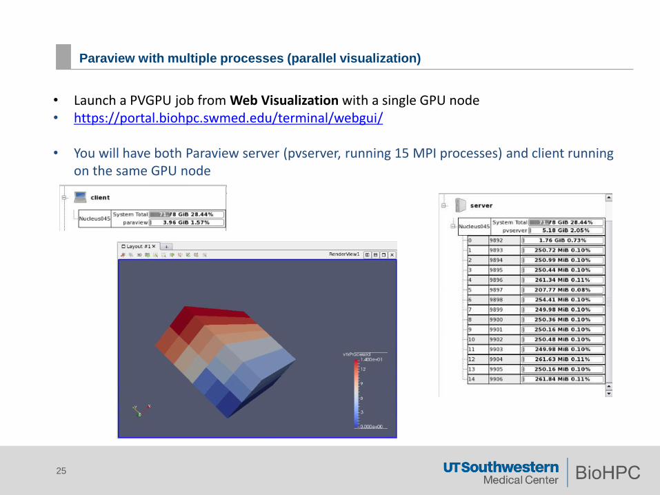
• Launch a PVGPU job from Web Visualization with a single GPU node• https://portal.biohpc.swmed.edu/terminal/webgui/
• You will have both Paraview server (pvserver, running 15 MPI processes) and client running on the same GPU node
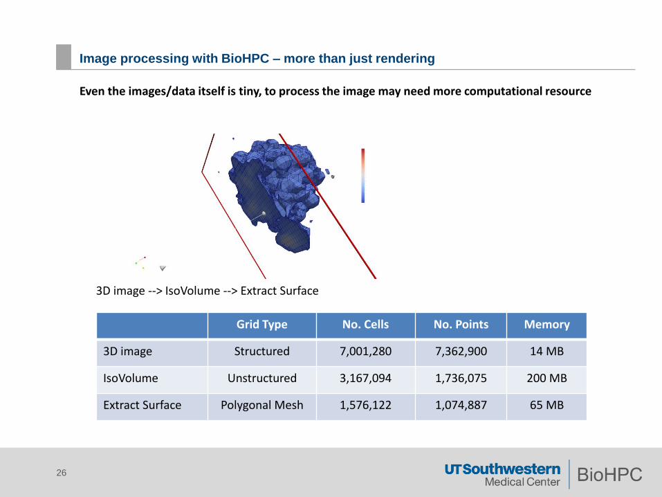
Image processing with BioHPC – more than just rendering
26
Even the images/data itself is tiny, to process the image may need more computational resource
3D image --> IsoVolume --> Extract Surface
Grid Type No. Cells No. Points Memory
3D image Structured 7,001,280 7,362,900 14 MB
IsoVolume Unstructured 3,167,094 1,736,075 200 MB
Extract Surface Polygonal Mesh 1,576,122 1,074,887 65 MB

Actual steps for bleb detection and tracking
27
Running time on one BioHPC node is ~ 15 mins

28
Image processing in a Parallel way : Vessel Extraction
microscopy image (size:2126*5517)
binary image243 subsets of binary image
local normalizationremove pepper & saltthreshold
separate vessel groups based on connectivity
find the central line of vessel (fast matching method)
~ 6.5 hours
~ 21.3 seconds
~ 6.6 seconds
* Images were provided by Woo-Ping Ge and Bo Ci

29
Matlab Distributed Computing Server
Vessel Extraction (step 3)
parfor i = 1 : length(numSubImages)% load binary imageI = im2double(Bwall(:,:i));% find vessel by using fast matching methodallS{i} = skeleton(I);
end
time needed for processing each sub image various Job running on 4 nodes requires minimum computational timet = 784 s
t = 784 s
Speedup = 28.3x
Last but not least
30
Please email the ticket system: [email protected]
For questions and comments
Acknowledgement
Meghan Driscoll, Denise Ramirez, Reto Fiolka, Kevin Dean, Erik Welf, Woo-Ping Ge, Bo Ci, Gaudenz Danuser, Philippe Roudot, Liqiang Wang, David Trudgian
• The primary goal of visualization is insight• Visualization system technology improves with advances in GPUs and HPC solutions• Challenges at every stage of visualization when operating on large data• We will continously working on delivery better visualization and analytic tools
Summary