University of Calgary

PRISM: University of Calgary's Digital Repository

Graduate Studies The Vault: Electronic Theses and Dissertations

2017

Visualization of Heavy Oil Chemical Flooding

Processes

Voroniak, Andrii

Voroniak, A. (2017). Visualization of Heavy Oil Chemical Flooding Processes (Unpublished

master's thesis). University of Calgary, Calgary, AB. doi:10.11575/PRISM/28650

http://hdl.handle.net/11023/3607

master thesis

University of Calgary graduate students retain copyright ownership and moral rights for their

thesis. You may use this material in any way that is permitted by the Copyright Act or through

licensing that has been assigned to the document. For uses that are not allowable under

copyright legislation or licensing, you are required to seek permission.

Downloaded from PRISM: https://prism.ucalgary.ca

UNIVERSITY OF CALGARY

Visualization of Heavy Oil Chemical Flooding Processes

by

Andrii Voroniak

A THESIS

SUBMITTED TO THE FACULTY OF GRADUATE STUDIES

IN PARTIAL FULFILMENT OF THE REQUIREMENTS FOR THE

DEGREE OF MASTER OF SCIENCE

GRADUATE PROGRAM IN CHEMICAL AND PETROLEUM ENGINEERING

CALGARY, ALBERTA

January, 2017

© Andrii Voroniak 2017

ii

Abstract

The observation made in laboratory core floods is that chemical recovery of oil is achieved

under high pressure gradients. A potential shortfall of core tests is their 1D nature: there are only

limited water pathways established throughout the core during the initial waterflood. In this case,

water channels can be blocked and the additional oil produced before chemical consequently

breaks through. In actual reservoirs, with more water pathways present, there is a possibility that

this blockage mechanism will not be significant, and production from chemical flooding may not

work the way it does in the laboratory.

This thesis presents a study on heavy oil production using chemicals in a 2D Hele-Shaw

cell system. This system does not allow for capillary trapping of fluids so localized water channel

blockage will not occur, and the cell is 2D so non-linear flow pathways can be visualized. Chemical

injections (surfactant, polymer and SP systems) are run in the Hele-Shaw cell with the goal being

to identify if there is still an improved recovery from chemical floods and, if so, to identify the

production mechanisms.

Keywords: viscous fingering, waterflooding, surfactant/polymer flooding, Hele-Shaw cell,

material balance, image processing

iii

Preface

This thesis includes materials (i.e. tables, figures, formulas and texts) from two Society of

Petroleum Engineers (SPE) conference papers:

1. Voroniak, A., Bryan, J. L., Hejazi, H., and Kantzas, A. 2016. Two-Dimensional

Visualization of Heavy Oil Displacement Mechanism During Chemical Flooding.

Paper SPE-181640-MS, presented at the SPE Annual Technical Conference and Exhibition

held in Dubai, UAE, 26-28 September.

2. Voroniak, A., Bryan, J. L., Taheri, S., Hejazi, H., and Kantzas, A. 2016. Investigation of

Post-Breakthrough Heavy Oil Recovery by Water and Chemical Additives Using Hele-

Shaw Cell. Paper SPE-181149-MS, presented at the SPE Latin America and Caribbean

Heavy and Extra Heavy Oil Conference held in Lima, Peru, 19-20 October.

iv

Acknowledgements

I would like to express my sincere appreciation to my supervisor, Dr. Apostolos Kantzas

for his guidance and encouragement, without which this work would not have been possible. I

would also like to thank my co-supervisor Dr. Hossein Hejazi for his helpful discussions during

this project.

I would like to thank Dr. Jonathan Bryan for his support provided in different stages of my

research.

I also would like to thank all the staff and students at the Fundamentals of Unconventional

Recourses (FUR) team, especially Dr. Saeed Taheri and Dr. Petro Babak.

I am grateful for the financial support from NSERC AITF/i-Core Industrial Research Chair.

Finally, I would like to thank my family for their continuous support throughout my life.

v

Table of Contents

Abstract ............................................................................................................................... ii

Preface................................................................................................................................ iii

Acknowledgements ............................................................................................................ iv

Table of Contents .................................................................................................................v

List of Tables .................................................................................................................... vii

List of Figures and Illustrations ....................................................................................... viii

List of Symbols, Abbreviations and Nomenclature ........................................................... xi

CHAPTER 1 ........................................................................................................................1

1 INTRODUCTION ......................................................................................................1

1.1 Background ..............................................................................................................1

1.2 Objective ..................................................................................................................7

1.3 Organization of the thesis ........................................................................................7

CHAPTER 2 ........................................................................................................................9

2 EXPERIMENTAL SETUP .........................................................................................9

2.1 Experimental procedure .........................................................................................11

2.2 Error Analysis ........................................................................................................14

CHAPTER 3 ......................................................................................................................19

3 WATERFLOODING ................................................................................................19

3.1 Heavy Oil Displacement by Water ........................................................................19

3.2 Waterflood Displacement Tests .............................................................................22

vi

CHAPTER 4 ......................................................................................................................28

4 SURFACTANT FLOODING ...................................................................................28

4.1 Surfactant Flooding Tests ......................................................................................28

CHAPTER 5 ......................................................................................................................35

5 POLYMER FLOODING ..........................................................................................35

5.1 Heavy Oil Displacement by Polymer ....................................................................35

CHAPTER 6 ......................................................................................................................42

6 SURFACTANT-POLYMER FLOODING ..............................................................42

6.1 Surfactant-Polymer Injection .................................................................................42

6.2 Surfactant and Surfactant-Polymer Injection at Low Shear Rates .........................47

6.3 Surfactant and Surfactant-Polymer Injection at High Shear Rates ........................54

CHAPTER 7 ......................................................................................................................62

7 CONCLUSIONS.......................................................................................................62

REFERENCES ..................................................................................................................64

APPENDIX A: RHEOLOGICAL PROPERTIES OF CHEMICAL SOLUTIONS..........70

APPENDIX B: COPYRIGHT PERMISSION LETTERS ................................................72

vii

List of Tables

Table 2-1. Viscosity of Surfactant (15,000 ppm), polymer (100 ppm) and SP (15,000 ppm; 100

ppm) at Various Flow Rates ................................................................................................. 13

Table 2-2. Reynolds Number Calculated for Injection Fluids at Different Velocities ................. 14

Table 2-3. Uncertainty measurement for waterflooding followed (0.3 cm³/min) by SP Flood

(4.8 cm³/min)......................................................................................................................... 16

Table 2-4. Recovery factors at the breakthrough, 1PV, 2PV, 3 PV and 4PV for the same 5 runs

............................................................................................................................................... 17

Table 2-5. Microsoft Excel output summary ................................................................................ 18

Table 2-6. Microsoft Excel output ANOVA Single Factor .......................................................... 18

Table 3-1. Waterflood Recovery Efficiency at Low and Intermediate Rates ............................... 21

Table 5-1. Polymer flood summary .............................................................................................. 40

Table 6-1. Low rate surfactant and SP injection summary ........................................................... 54

Table 6-2. High rate surfactant and SP injection summary .......................................................... 61

viii

List of Figures and Illustrations

Figure 1-1. Distribution of Heavy Oil, Bitumen and Oil Shale Resources Globally. Source:

Harraz, 2016 ........................................................................................................................... 1

Figure 1-2. Microscopic Displacement during Waterflooding. Source: Oilfield Review, Winter

2010/2011 ............................................................................................................................... 2

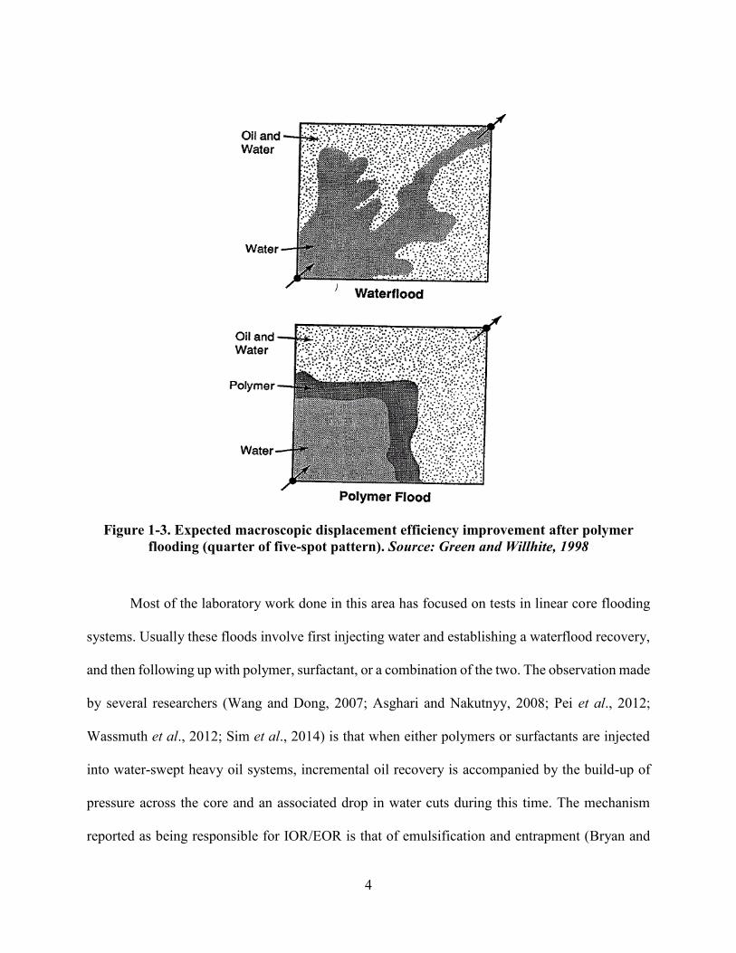
Figure 1-3. Expected macroscopic displacement efficiency improvement after polymer

flooding (quarter of five-spot pattern). Source: Green and Willhite, 1998 ............................ 4

Figure 1-4. Pore level discplacement during alkaline-surfactant-polymer flooding. Source:

Sedaghat et al., 2015 ............................................................................................................... 5

Figure 2-1. Hele-Shaw Cell (isometric view) ................................................................................. 9

Figure 3-1. Comparison of waterflood images for injection rate of 0.1 cm³/min (top row) and

0.6 cm³/min (bottom row) ..................................................................................................... 19

Figure 3-2. Recovery profile based on image analysis and material balance ............................... 21

Figure 3-3. Waterflood images for injection rate of 0.1 cm³/min (top) and 0.6 cm³/min (bottom)

............................................................................................................................................... 24

Figure 3-4. Oil production profiles at two different water injection rates .................................... 25

Figure 3-5. Waterflood images for injection rate of 4.8 cm³/min ................................................. 26

Figure 3-6. Waterflood at 0.6 cm³/min until breakthrough and then 4.8 cm³/min. ...................... 27

ix

Figure 4-1. Images of surfactant bottle testing at different concentrations: from left to right

7500 ppm, 10,000 ppm, 12,500 ppm and 15,000 ppm ......................................................... 29

Figure 4-2. Images showing waterflood followed by high rate surfactant building emulsions

(4.8 cm³/min)......................................................................................................................... 31

Figure 4-3. Recovery profile of water (4.8 cm³/min) vs. surfactant (4.8 cm³/min) ...................... 31

Figure 4-4. Images comparing emulsion sweep to polymer sweep at high injection rate of 4.8

cm³/min ................................................................................................................................. 33

Figure 4-5. Recovery profile of water followed by high rate polymer vs. high rate surfactant ... 34

Figure 5-1. Images of polymer flooding (top, middle) and waterflooding (bottom) at different

injection rates. ....................................................................................................................... 37

Figure 5-2. Polymer response compared to water ........................................................................ 38

Figure 5-3. Waterflood followed by polymer vs. waterflood ....................................................... 39

Figure 5-4. Comparison of breakthrough and post-breakthrough recovery for waterflooding

and polymerflooding ............................................................................................................. 40

Figure 5-5. Polymer flooding vs. waterflooding followed by polymer flooding .......................... 41

Figure 6-1. Images of surfactant vs. SP bottle test ....................................................................... 43

Figure 6-2. Images of water followed by high rate surfactant and SP solution ............................ 44

Figure 6-3. Recovery profile of water and high rate surfactant vs. water and high rate SP ......... 46

x

Figure 6-4. Recovery profile of high rate of SP vs. intermediate rate of polymer ....................... 47

Figure 6-5. Images of surfactant and SP injection at 0.6 cm³/min ................................................ 49

Figure 6-6. Images taken at breakthrough during waterflooding and surfactant flooding at 0.6

cm³/min ................................................................................................................................. 50

Figure 6-7. Low rate injection (0.6 cm³/min) of surfactant, polymer and water .......................... 51

Figure 6-8. Water followed by polymer vs. water flowed by SP ................................................. 53

Figure 6-9. Water, surfactant, polymer and SP at lower shear rates ............................................. 54

Figure 6-10. Images of surfactant, surfactant-polymer and water injection at 0.6 cm³/min ......... 56

Figure 6-11. Comparison of two different surfactant flooding scenarios ..................................... 58

Figure 6-12. Water followed by a high rate surfactant and SP solution ....................................... 59

Figure 6-13. Water followed by a high rate chemical solutions ................................................... 60

Figure 6-14. Comparison of surfactant, polymer and SP injection at high shear rates ................. 61

xi

List of Symbols, Abbreviations and Nomenclature

Symbol Definition

E Overall displacement efficiency

ED Microscopic displacement efficiency

EV Macroscopic (volumetric) displacement efficiency

h Distance between plates in the Hele-Shaw cell [m]

Lx Width of the Hele-Shaw cell [m]

M Viscosity ratio between oil and injection fluid

𝑁𝑔 Gravity number

O/W Oil-in-water

OOIP Original Oil-in-Place

P Polymer

PV Pore volume

Re Reynolds number

S Surfactant

SP Surfactant-polymer

v Superficial velocity [m/s]

𝜐 Injection fluid velocity [m/s]

Greek letters

μ Injection fluid viscosity [Pa·s]

𝜇𝑤 Viscosity of water [Pa·s]

Injection fluid density [kg/m³]

ow Interfacial tension between oil and injection fluid [N/m]

xii

𝛾𝑎𝑐𝑡𝑢𝑎𝑙 Actual shear rate from flow at a fixed rate [𝑠−1]

𝑘 Absolute permeability

𝜙 Absolute porosity

1

CHAPTER 1

1 INTRODUCTION

1.1 Background

Canada possesses significant amount of unconventional resources (Figure 1-1). Many of its

heavy oil deposits are contained in relatively small and thin sands. Heavy oil sand porosity and

permeability are high, with order of magnitude 30% and 1 D (Jardine, 1974). Heavy oil reservoirs

are a subset of this resource base, where oil is highly viscous, yet having some limited mobility at

reservoir temperature and pressure. Most of these reservoirs are produced by either cold production

(Dusseault, 2002) or through a combination of primary production and waterflooding (Kumar et

al., 2005; Miller, 2006; Vittoratos et al., 2007; Mai and Kantzas, 2009).

Figure 1-1. Distribution of Heavy Oil, Bitumen and Oil Shale Resources Globally. Source:

Harraz, 2016

2

At the end of primary production there is still 85-95% of the original oil resource left in

place, but thermal methods are challenging or even impossible in these systems. Many heavy oil

pools are or can possibly be waterflooded, but displacement of heavy oil by water is inefficient

and slow. This is due to the fact that some oil blobs can be trapped within a pore or a group of

pores that are connected (Figure 1-2). Chemical flooding is considered as a means for improving

the response of waterflooding, and there has been considerable work done in recent years showing

the potential for surfactant flooding (Santanna, 2009; Huang and Dong, 2004; Kumar and

Mohanty, 2011) and polymer flooding (Seright, 2010; Wang et al., 2010; Sheng, 2011) in heavy

oil systems.

Figure 1-2. Microscopic Displacement during Waterflooding. Source: Oilfield Review,

Winter 2010/2011

Displacement of heavy oil by water is an unstable process, where injected water tends to

finger through preferred channels, thereby by-passing significant volumes of oil bearing reservoir.

Generally, heavy oil production by waterflooding is accompanied by large volumes of produced

water (Beliveau, 2009). Historically, low temperature enhanced recovery systems such as

waterflooding have proved to be an effective, low cost means to attain increased oil recovery.

There are field pilots already ongoing considering polymer flooding in heavy oil pools (Wassmuth

et al., 2009; Delamaide et al., 2013) and multiple laboratory studies looking at alkali and surfactant

3

injection have also been carried out (Liu et al., 2006; Bryan and Kantzas, 2008; Hunky et al.,

2010). These studies show promising improvement in oil recovery, suggesting exciting future low

cost production possibilities.

On a microscopic scale we can determine displacement efficiency of water displacing oil

from a porous medium. The same approach is used when water-oil flow measurements are made

on core sample in lab conditions. In order to get accurate results of recovery by enhanced oil

recovery methods on a reservoir scale the effects of geology, gravity, and geometry (vertical,

areal, well-spacing/pattern arrangement) should be included. The overall displacement efficiency

of any oil recovery displacement process is a combination of microscopic and macroscopic

displacement efficiencies (Green and Willhite, 1998):

𝐸 = 𝐸𝐷𝐸𝑉 Eq. 1.1

where E – overall displacement efficiency, ED – microscopic displacement efficiency,

and EV – macroscopic (volumetric) displacement efficiency.

Microscopic displacement is responsible for oil mobilization at the pore scale. Macroscopic

displacement is related to the effectiveness of the displacement in terms of volume (sweep

efficiency).

4

Figure 1-3. Expected macroscopic displacement efficiency improvement after polymer

flooding (quarter of five-spot pattern). Source: Green and Willhite, 1998

Most of the laboratory work done in this area has focused on tests in linear core flooding

systems. Usually these floods involve first injecting water and establishing a waterflood recovery,

and then following up with polymer, surfactant, or a combination of the two. The observation made

by several researchers (Wang and Dong, 2007; Asghari and Nakutnyy, 2008; Pei et al., 2012;

Wassmuth et al., 2012; Sim et al., 2014) is that when either polymers or surfactants are injected

into water-swept heavy oil systems, incremental oil recovery is accompanied by the build-up of

pressure across the core and an associated drop in water cuts during this time. The mechanism

reported as being responsible for IOR/EOR is that of emulsification and entrapment (Bryan and

5

Kantzas, 2007) with emulsion or polymer plugs blocking off pre-formed water channels, thus

leading to improved sweep efficiency in the core.

Figure 1-4. Pore level discplacement during alkaline-surfactant-polymer flooding. Source:

Sedaghat et al., 2015

A potential shortfall of core tests is their 1D nature: there are only limited water pathways

established throughout the core during the initial waterflood. In these systems, it is possible for

water channels to be blocked and then additional oil is produced before chemical breaks through

a second time. For small core systems, this incremental production can be significant when

expressed in terms of original oil in place volumes. In actual reservoirs, with infinitely more water

pathways present, it is possible that this blockage mechanism will not be as significant, and

production from chemical injection may not work the way it does in the laboratory. The linear

nature of these floods is emphasized, because in these cores there are only limited pathways for

water and oil to flow. Injection of chemical needs only to block off some of these pathways and

pressure will once again build up across the core and lead to incremental oil production. This was

shown in past tests run in parallel cores (Bryan et al., 2013), wherein surfactant and polymer

6

injection only led to increased recovery in the highest permeability core and left the lower

permeability system still upswept. In the field, there are many more flow paths present than what

is present in a linear core flood, and so the improvement from chemical flooding may be

overemphasized in the laboratory. The primary objective of this study was to run tests in 2D

systems, where the impact of localized blockages and flow diversion would be minimized. Within

this new configuration, tests were run with the goal of imaging displacement and

understanding/visualizing chemical production mechanisms.

Flow in porous media is a difficult problem of great importance. Since it is not possible to

see into the porous medium, many researchers have found a way to visualize the flow in the

reservoir employing such tools as glass micromodels, glass bead packs and Hele-Shaw cells

(Engelberts and Klinkenberg, 1951; Chatenever and Calhoun, 1952; Brock and Orr Jr., 1991;

Hornoff and Morrow, 1988; Kong et al., 1992; Xianli et al., 1992). Such models lack important

3D aspects and do not account for gravity when placed horizontally, but they provide insight on

the micromechanics of the displacement. The Hele-Shaw cell used in this study does not allow for

capillary trapping of fluids and plugging from emulsions being trapped in pore throats, so any

chemical mechanisms studied are expected to be present and significant at a much wider scale than

just localized plugging of pores. The cell is named after one of the most prominent researchers in

applied sciences and engineering Henry Selby Hele-Shaw (1854-1941). This device allows us to

investigate two-dimensional flow of a viscous fluid in a small gap between two parallel plates. The

motion in the Hele-Shaw cell is similar to two-dimensional flow in a porous medium.

This thesis presents a study on heavy oil production using chemicals in a 2D Hele-Shaw cell

system. This system has no capillary trapping of fluids, so localized water channel blockage will

not occur, and the cell is 2D so non-linear flow pathways can also be visualized. Chemical floods

7

(polymer, surfactant and SP systems) are run in this cell and the goal is to identify if there is still

an improved recovery from chemical injection and, if so, what production mechanisms are

responsible for this recovery.

1.2 Objective

There is ample data showing the potential for heavy oil recovery from injection of water and

chemical additives (polymer, surfactant and SP systems). Most of this data has been acquired in

linear cores, and as a result the relative impact of these chemical additives on incremental oil

recovery is potentially overly emphasized compared to what is seen in the field. In order to better

understand the mechanisms of heavy oil displacement in a 2D system without emphasis on

localized flow re-diversion, tests were run in a 2D Hele-Shaw cell (no pore-scale trapping). By

comparing the sweep efficiency during water and chemical addition, the impact of surfactants and

polymers can be better understood.

The 2D system allows for an understanding of whether chemicals sweep incremental oil

from along the same channels as the pre-formed water or if new displacement channels are formed.

Also, by running tests in the Hele-Shaw cell, results can be compared against core flooding data

from the literature. The improved displacement in this cell can be compared against the relative

improvement from core floods in order to infer whether recovery is related to improved sweep or

if localized blockage and flow re-diversion are the main contributors to improved oil recovery

from chemicals.

1.3 Organization of the thesis

The thesis is divided into a total of 7 chapters. Chapter 1 covers the background information

on chemical flooding previously performed in laboratory conditions. Emphasis is given to core

8

flooding experiments in heavy oil systems. Chapter 2 provides with the details of experiments as

well as with the materials and methods used to post process the results. The baseline study for

heavy oil displacement test is presented in waterlooding section, which is Chapter 3. Actual

surfactant flooding, polymer flooding and SP flooding experiments are given in Chapters 4, 5 and

6 respectively.

Finally, conclusions. were drawn from this study based on experimental results.

Recommendations for the future work, which can enhance the understanding of the subject matter

are discussed. These can be found in Chapter 7.

The main contribution of the work is running two dimensional tests instead of linear core

floods. The Hele-Shaw cell allows for an understanding of whether chemicals sweep incremental

oil from along the same channels as the pre-formed water or if new displacement channels are

formed. Also, by running tests in the Hele-Shaw cell, which does not allow for trapping,

observations can be made regarding whether trapping and fluid re-diversion are the only ways that

these chemicals can yield improved oil recovery, or if simple alteration of the mobility ratio

without additional trapping will already lead to incremental oil.

9

CHAPTER 2

2 EXPERIMENTAL SETUP

The Hele-Shaw cell created for these oil displacement experiments was constructed from

Plexiglass. The two flat parallel plates were separated by a Teflon gasket and held together with

20 bolts (Figure 2-1). The cell has dimensions of 28 cm x 21.5 cm. The plates are separated by a

gap of 0.039 cm and the thickness of each glass plate is 2.54 cm. Injection of fluids is through the

top right corner of the model, and production is from the bottom left corner providing a diagonal

flow path through the system with a variable cross-sectional area. This in turn allows for

visualization of fingering and bypassing during displacement tests.

Figure 2-1. Hele-Shaw Cell (isometric view)

10

The test procedure was to first vacuum saturate the Hele-Shaw cell with water and then inject

oil at constant rate (0.5 cm³/min) through the cell in order to saturate the cell with oil and just a

residual water film present. Fluids were injected by using an ISCO Model 500D pump through the

top right port of the cell. This pump was operated under a few constant flow-rate conditions: 0.1

cm³/min, 0.6 cm³/min and 4.8 cm³/min. The produced fluids were discharged at ambient conditions

through the left bottom port, and collected in 25 cm³ glass graduated cylinders (or vials) having

0.5 cm³ gradation markings. Production samples were acquired at fixed intervals within each flood,

and oil and water within each sample was visually measured to obtain the material balance

cumulative oil production as a function of pore volumes (PV) water or chemical injected.

In addition to material balance measurements of recovery, images were also acquired

throughout each flood using a high resolution digital camera (Nikon Coolpix P520, 18.1

Megapixels). The oil was dyed red (Sudan red G, Sigma-Aldrich Corporation) and therefore in

these images red regions in the cell are oil and white regions show the injection fluid, i.e. oil that

has been displaced out of the cell. The images were later analyzed using the ImageJ (National

Institute of Health, Version 1.49v) software package, an image manipulation software. Images

were thresholded into binary pictures and the displaced oil fraction was measured directly from

each picture. Images can allow for visualization of the nature of displacement, while binarizing

the images allows for quantification of oil recovery and comparison against material balance.

The oil phase used in this study is viscous mineral oil (1015 mPa·s at 23°C). Water floods

(and initial cell water saturation) are run with distilled water. The polymer used in this system is

an anionic HPAM made by Kemira Chemicals Canada Inc. (KemSweep A-5360). A polymer

concentration of 100 ppm was used in this study: low polymer concentration was needed in order

to obtain reasonable viscosity values under the low shear present in the Hele-Shaw cell. The

11

surfactant used is a commercial product (HORA-W805) supplied by ChemEOR Inc. The surfactant

concentration used in displacement tests is 15,000 ppm.

2.1 Experimental procedure

Tests are performed in a 2D visual Hele-Shaw cell, where a sample of viscous mineral oil

(1015 mPa·s at 23°C) is displaced by water, polymer and SP systems at various flow rates. The

experiments are run for multiple pore volumes, to study growth and distribution of fingers before

and after water breakthrough. With the addition of chemical (polymer, surfactant or SP) after

waterflooding vs. without previous waterflooding, the effect of parameters such as the fluid

viscosity ratio or emulsification and entrainment of oil can be studied. Production samples are

taken periodically and images taken at higher frequency. The material balance and image

processing techniques are used to post-process the results.

The efficiency of each flooding scenario is analyzed in terms of cumulative oil recovery vs. PV

injected from material balance and from image analysis. Images show the fraction of the model

that has been completely swept by the invading phase (water or chemical) while the material

balance data includes the potential for flow of oil and water within the same channel. This

comparison allows for an understanding of how viscous oil is displaced by water, i.e. by viscous

displacement of oil out of the model through a continuous water pathway, or by flowing oil and

water together as in the case of emulsion flow.

The oil/injection fluid viscosity ratio is consistently much higher than 1. Calculated

Instability Number values (Bentsen, 1985) are much greater than 10, so displacement of 1015

mPas oil by any of these injection fluids is an unstable process. Improvements in recovery from

chemical flooding compared to water are not related to the flood becoming stable, so viscous

fingering will be expected to always be present in all tested systems.

12

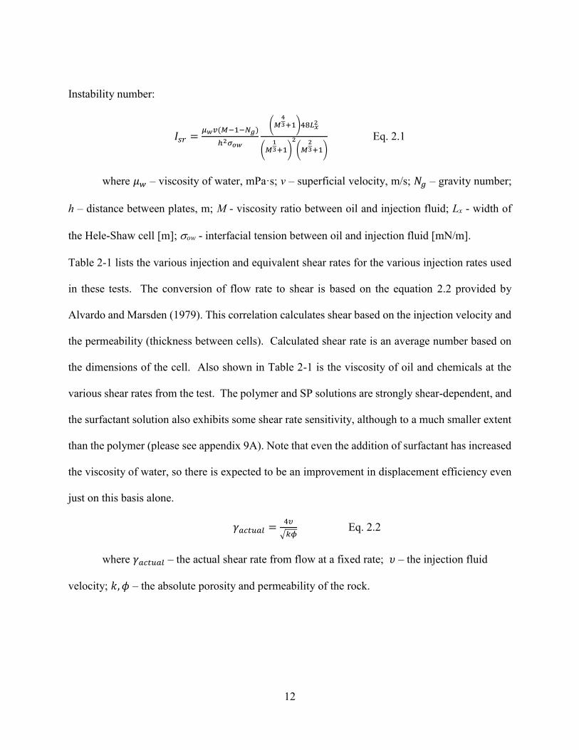
Instability number:

𝐼𝑠𝑟 =𝜇𝑤𝑣(𝑀−1−𝑁𝑔)

ℎ2𝜎𝑜𝑤

(𝑀43+1)48𝐿𝑥

2

(𝑀13+1)

2

(𝑀23+1)

Eq. 2.1

where 𝜇𝑤 – viscosity of water, mPa·s; v – superficial velocity, m/s; 𝑁𝑔 – gravity number;

h – distance between plates, m; M - viscosity ratio between oil and injection fluid; Lx - width of

the Hele-Shaw cell [m]; ow - interfacial tension between oil and injection fluid [mN/m].

Table 2-1 lists the various injection and equivalent shear rates for the various injection rates used

in these tests. The conversion of flow rate to shear is based on the equation 2.2 provided by

Alvardo and Marsden (1979). This correlation calculates shear based on the injection velocity and

the permeability (thickness between cells). Calculated shear rate is an average number based on

the dimensions of the cell. Also shown in Table 2-1 is the viscosity of oil and chemicals at the

various shear rates from the test. The polymer and SP solutions are strongly shear-dependent, and

the surfactant solution also exhibits some shear rate sensitivity, although to a much smaller extent

than the polymer (please see appendix 9A). Note that even the addition of surfactant has increased

the viscosity of water, so there is expected to be an improvement in displacement efficiency even

just on this basis alone.

𝛾𝑎𝑐𝑡𝑢𝑎𝑙 =4𝜐

√𝑘𝜙 Eq. 2.2

where 𝛾𝑎𝑐𝑡𝑢𝑎𝑙 – the actual shear rate from flow at a fixed rate; 𝜐 – the injection fluid

velocity; 𝑘, 𝜙 – the absolute porosity and permeability of the rock.

13

Table 2-1. Viscosity of Surfactant (15,000 ppm), polymer (100 ppm) and SP (15,000 ppm;

100 ppm) at Various Flow Rates

Injection rate, cm³/min 0.1 0.6 4.8

Equivalent shear rate, s-1 0.71 4.24 33.90

Viscosity of water, mPa·s 1 1 1

Viscosity of surfactant, mPa·s 4.5 3.6 2.8

Viscosity of polymer, mPa·s 44 21 8.9

Viscosity of surfactant-polymer, mPa·s 26.2 15.7 8.7

Oil/water viscosity ratio 1015 1015 1015

Oil/surfactant viscosity ratio 226 282 363

Oil/polymer viscosity ratio 23 48 114

Oil/SP viscosity ratio 39 65 117

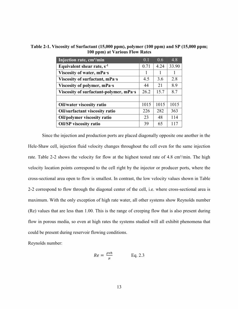
Since the injection and production ports are placed diagonally opposite one another in the

Hele-Shaw cell, injection fluid velocity changes throughout the cell even for the same injection

rate. Table 2-2 shows the velocity for flow at the highest tested rate of 4.8 cm³/min. The high

velocity location points correspond to the cell right by the injector or producer ports, where the

cross-sectional area open to flow is smallest. In contrast, the low velocity values shown in Table

2-2 correspond to flow through the diagonal center of the cell, i.e. where cross-sectional area is

maximum. With the only exception of high rate water, all other systems show Reynolds number

(Re) values that are less than 1.00. This is the range of creeping flow that is also present during

flow in porous media, so even at high rates the systems studied will all exhibit phenomena that

could be present during reservoir flowing conditions.

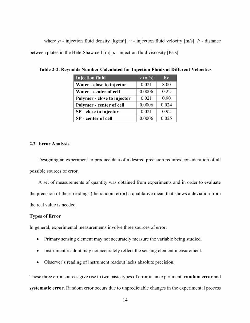
Reynolds number:

𝑅𝑒 = 𝜌𝜈ℎ

𝜇 Eq. 2.3

14

where - injection fluid density [kg/m³], v - injection fluid velocity [m/s], h - distance

between plates in the Hele-Shaw cell [m], μ - injection fluid viscosity [Pa s].

Table 2-2. Reynolds Number Calculated for Injection Fluids at Different Velocities

Injection fluid v (m/s) Re

Water - close to injector 0.021 8.00

Water - center of cell 0.0006 0.22

Polymer - close to injector 0.021 0.90

Polymer - center of cell 0.0006 0.024

SP - close to injector 0.021 0.92

SP - center of cell 0.0006 0.025

2.2 Error Analysis

Designing an experiment to produce data of a desired precision requires consideration of all

possible sources of error.

A set of measurements of quantity was obtained from experiments and in order to evaluate

the precision of these readings (the random error) a qualitative mean that shows a deviation from

the real value is needed.

Types of Error

In general, experimental measurements involve three sources of error:

Primary sensing element may not accurately measure the variable being studied.

Instrument readout may not accurately reflect the sensing element measurement.

Observer’s reading of instrument readout lacks absolute precision.

These three error sources give rise to two basic types of error in an experiment: random error and

systematic error. Random error occurs due to unpredictable changes in the experimental process

15

(for instance, measuring instruments or environmental conditions). Systematic error is associated

with measuring instrument (the device is not properly calibrated or experimenter used it wrongly).

All laboratory measurements are subject to experimental error. Absolute accuracy is not possible

when taking measurements.

With reference to the specific experimental process described in this thesis, the source of

error can be summarized as follows:

Pump Error: Pump manufacturer’s stated flow rate accuracy (0.001

cm³/min), multiplied by total injection time (minutes) for the

test.

Hele Shaw Cell Saturation Error: Error derives from compressibility of the Teflon gasket

placed between the two plates. The bolts were tightened

manually for each test, thereby generating slightly different

thickness between the two plates. Therefore, pore volume

variation for each test resulted from Teflon compressibility.

Error from this source was calculated based on observed

variations in pore volume, from which standard deviations

were calculated.

Vial Error: Measurement of recovered fluids from the cell was made in

a vertical, graduated glass cylinder (vial). The error of

measurement is considered to be half of the smallest division

on the instrument scale, which was 0.5 cm³. Therefore, the

error is 0.25 cm³.

Total Error of Measurement = [Pump Error] + [Hele-Shaw Cell Saturation Error] + [Vial Error]

16

Total Error of Measurement = [Flow Rate Accuracy of the Pump] * [injection time] + [Standard

Deviation of a Pore Volume] + [Half of the Smallest Division of the Vial]

Total Error Measurement (cm³) = [0.001 cm³/min] * [injection time] + [0.085 cm³] +

[0.25 cm³]

The Table 2-3 shown below is a compilation of total error, and is an example of total

measurement of error for each run. The error was calculated as described above.

Table 2-3. Uncertainty measurement for waterflooding followed (0.3 cm³/min) by SP Flood

(4.8 cm³/min)

PV V,

cm³

Rate,

cm³/min

Time,

min

Pump Error,

cm³

Total Error,

cm³

Total Error,

%

0.00 0 0.3 0 0 0 0

0.40 8.6 0.3 29 0.03 0.36 1.73

1.00 21.5 0.3 72 0.07 0.41 1.94

2.02 43.3 4.8 76 0.08 0.41 1.96

3.02 65.0 4.8 81 0.08 0.42 1.97

4.00 85.9 4.8 85 0.09 0.42 2.00

5.00 107.5 4.8 90 0.09 0.42 2.02

Analysis of experimental data and associated errors show the conclusions made from

experimental data to be unaffected by these calculated levels of error.

When comparing material balance data and image processing data, the recovery differences

are inside the range of uncertainty shown by the error bars in the material balance. Thus, obtained

oil recovery is the same for both methods.

17

Reproducibility of the results for same runs

Same five waterflooding experiments were run in order to test the reproducibility of the

results. One-Way Analysis of Variance (ANOVA) is used in order to compare the means of the

groups (runs).

Based on previously run five same waterflooding experiments at 0.6 cm³/min, recovery

factors (RF) were calculated at points of specific pore volume injected (PV). Results are given in

Table 2-4.

Table 2-4. Recovery factors at the breakthrough, 1PV, 2PV, 3 PV and 4PV for the same 5

runs

PV RF1, % RF2, % RF3, % RF4, % RF5. %

0.21 23.40 22.13 21.28 21.28 21.70

1 29.79 30.64 23.40 31.91 30.21

2 38.30 37.02 36.17 38.30 34.47

3 44.68 43.83 37.23 44.68 40.85

4 46.81 50.21 39.36 46.81 42.98

In ANOVA, we subdivide the total variation in the outcome measurements into that which

is attributable to differences among the groups and due to chance or attributable to inherent

variation within groups.

Hypothesis:

H0: all runs have the same means

H1: there are different means for some runs

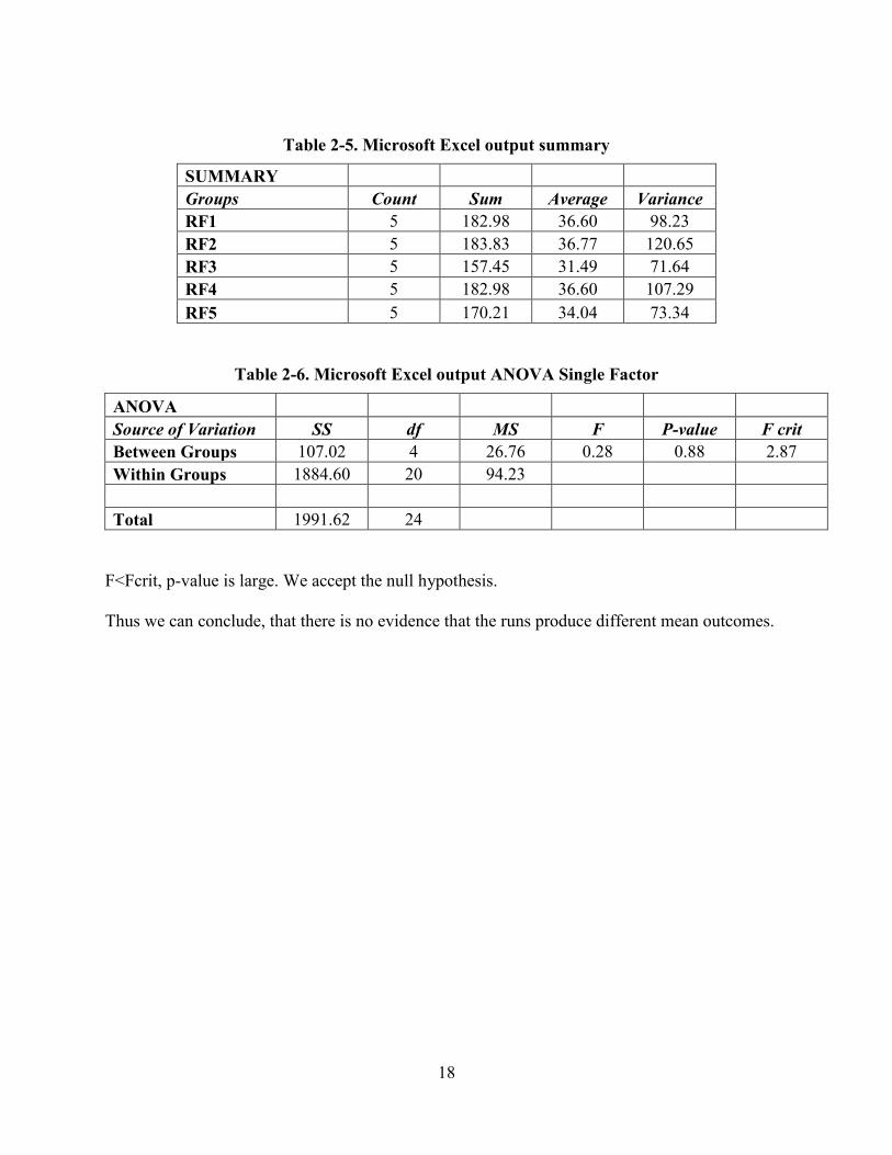
Tables 2-5 and 2-6 depict Microsoft Excel output of the ANOVA summary table for the five same

waterflooding runs.

18

Table 2-5. Microsoft Excel output summary

SUMMARY

Groups Count Sum Average Variance

RF1 5 182.98 36.60 98.23

RF2 5 183.83 36.77 120.65

RF3 5 157.45 31.49 71.64

RF4 5 182.98 36.60 107.29

RF5 5 170.21 34.04 73.34

Table 2-6. Microsoft Excel output ANOVA Single Factor

ANOVA

Source of Variation SS df MS F P-value F crit

Between Groups 107.02 4 26.76 0.28 0.88 2.87

Within Groups 1884.60 20 94.23

Total 1991.62 24

F<Fcrit, p-value is large. We accept the null hypothesis.

Thus we can conclude, that there is no evidence that the runs produce different mean outcomes.

19

CHAPTER 3

3 WATERFLOODING

3.1 Heavy Oil Displacement by Water

Figure 3-1 shows Hele-Shaw images of oil displaced by water at low and intermediate rates

of flow, 0.1 cm³/min and 0.6 cm³/min, respectively. Images are shown at the point of water

breakthrough, after 1 PV injection and at the end of the test (i.e. after 4 PV water injection). At the

point of breakthrough, water has fingered through the oil in both systems, so breakthrough occurs

with most of the oil in the cell still continuous and able to be produced.

W 0.1

W 0.6

Breakthrough 1PV injected End of the test

Figure 3-1. Comparison of waterflood images for injection rate of 0.1 cm³/min (top row)

and 0.6 cm³/min (bottom row)

20

The degree of fingering appears to be greater under the faster injection rate, which

corroborates with theories of instability and viscous fingering (Coskuner and Bentsen, 1988). The

effect of fingering on recovery efficiency is summarized in Figure 3-2 and in Table 3-1. Figure 3-

2 shows the solid lines are the recovery profiles as determined by analysis of images taken at

frequent intervals over the length of the flood. The points and error bars are from material balance

(i.e. collected fluid samples taken periodically through the flood). The first material balance point

is taken at the visualized water breakthrough, and subsequently samples are taken at the end of

each pore volume (PV) injected. The recovery at breakthrough is higher for the slower

displacement rate waterflood, and this result is verified by both images and material balance.

Higher displacement tests are more unstable for the same viscosity ratio (Bentsen, 1985) so the

lower recovery at 0.6 cm³/min is an expected result.

21

Figure 3-2. Recovery profile based on image analysis and material balance

Table 3-1. Waterflood Recovery Efficiency at Low and Intermediate Rates

Injection rate, cm³/min 0.1 0.6

Breakthrough recovery, % 36.33 25.13

Total recovery at 4 PV Inj, % 44.25 38.69

RF/PV after 1PV (% OOIP/PV) 2.25 2.86

Surprisingly, by the end of the 4 PV water injection, the total recovery from both systems

is closer than the recovery at the point of water breakthrough. This is further illustrated in Table

3-1, which shows the slope of the later time recovery after breakthrough (i.e. incremental oil

recovery / incremental PV injected). The higher rate waterflood has a slightly larger slope

compared to the 0.1 cm³/min injection rate. This result is opposite to what is observed in linear

22

heavy oil waterfloods (Mai and Kantzas, 2008). In porous media, lower injection rate leads to less

channeling of water and allows for an increased impact of capillary imbibition of water away from

swept zones. In this 2D Hele-Shaw cell, these capillary forces are insignificant. Instead, the result

of the higher post-breakthrough recovery slope at 0.6 cm³/min is due the fact that in this system,

water fingers pinched off and became discontinuous. When this happened, further injection of

water displaced more of the mobile oil, and this is responsible for the oil production bump at 2.2

PV injection in Figure 3-2. At lower injection rates this water channel snaps off and the re-

generation of oil displacement phenomenon was not as prevalent.

The slightly higher recovery slope from the post-breakthrough water injection test at 0.6

cm³/min is a reflection of viscous forces in the Hele-Shaw cell, i.e. better displacement of oil under

higher pressure gradients from the faster flow rate. However, while this may be an observation just

from the Hele-Shaw system, it still illustrates post-breakthrough recovery in heavy oil waterfloods.

The key to continued oil recovery beyond water breakthrough is that the oil is still continuous

within the reservoir. During water injection, fluids are constantly redistributing due to water

imbibition and changes in sweep patterns in active floods. This redistribution allows continuous

and mobile oil to be displaced and as a result heavy oil waterfloods can be run for years with

continuous oil cuts (Smith, 1992; Alvarez and Sawatzky, 2013).

3.2 Waterflood Displacement Tests

Figure 3-3 shows Hele-Shaw cell images of displacement of oil by constant injection rate of

water at 0.1 cm³/min, and also at 0.6 cm³/min. The clear regions of the cell are invaded water zones

as compared to the red areas shown in the images, which reflect red dye that has been placed in

the oil. Looking just at the images up to the point of breakthrough, the higher injection rate clearly

23

leads to the buildup of more and smaller fingers, since displacement is more unstable in this

system. Breakthrough recovery in Figure 3-4 is shown as the point where the slope of oil recovery

vs. PV injected reduces sharply. As expected, the breakthrough oil recovery is higher for the slower

displacement system that has fewer fingers, which is well documented in theories of viscous

fingering (Saffman and Taylor, 1958; van Meurs, 1959; Wooding, 1960).

The observation of greater significance is the nature of the water displacing zone after the

point of breakthrough. For both injection rates it appears that the pre-formed water pathways

eventually get broken up and later new breakthrough pathways are formed. This is shown as the

point labeled “Secondary breakthrough” in Figure 3-3. This observation means that once water

pathways form, continued injection will not necessarily just follow pre-existing pathways but

instead, water channels snap off and become surrounded by oil. When this happens, further

injection of water is now once again displacing continuous oil and this leads to additional

production of oil after the point of water breakthrough. This is illustrated in Figure 3-4.

24

0.1

0.6

Breakthrough 1 PV

Secondary

breakthrough

End of the test

Figure 3-3. Waterflood images for injection rate of 0.1 cm³/min (top) and 0.6 cm³/min

(bottom)

25

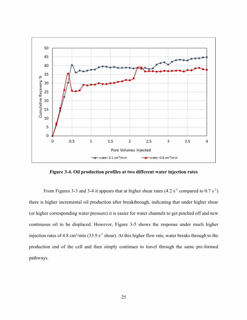
Figure 3-4. Oil production profiles at two different water injection rates

From Figures 3-3 and 3-4 it appears that at higher shear rates (4.2 s-1 compared to 0.7 s-1)

there is higher incremental oil production after breakthrough, indicating that under higher shear

(or higher corresponding water pressure) it is easier for water channels to get pinched off and new

continuous oil to be displaced. However, Figure 3-5 shows the response under much higher

injection rates of 4.8 cm³/min (33.9 s-1 shear). At this higher flow rate, water breaks through to the

production end of the cell and then simply continues to travel through the same pre-formed

pathways.

26

1.5 PV 2.5 PV 3.5 PV 4.5 PV

Figure 3-5. Waterflood images for injection rate of 4.8 cm³/min

Figure 3-6 shows the oil recovery profile for the high rate water injection, compared to the

previous intermediate rate flood. The breakthrough recovery appears to be only slightly lower than

the recovery for 0.6 cm³/min, which could be an indication that for both rates the flood is so highly

unstable that recovery once again does not change significantly with rate (Bentsen, 1985). When

shear rates are very high, however, the path of least resistance is through the same pre-formed

water channels and there is no more driving force for oil production at later times. For this reason,

oil recovery remains essentially unchanged with continued flooding, compared to the recovery

response at lower shear rates.

27

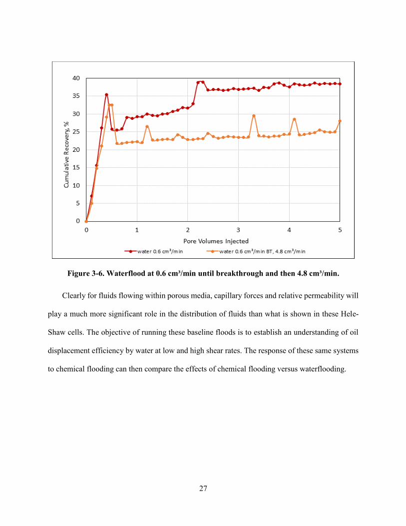
Figure 3-6. Waterflood at 0.6 cm³/min until breakthrough and then 4.8 cm³/min.

Clearly for fluids flowing within porous media, capillary forces and relative permeability will

play a much more significant role in the distribution of fluids than what is shown in these Hele-

Shaw cells. The objective of running these baseline floods is to establish an understanding of oil

displacement efficiency by water at low and high shear rates. The response of these same systems

to chemical flooding can then compare the effects of chemical flooding versus waterflooding.

28

CHAPTER 4

4 SURFACTANT FLOODING

4.1 Surfactant Flooding Tests

Laboratory test runs were made using the commercial heavy oil surfactant SurFlood HORA-

W805 provided for testing by ChemEOR Inc. Several surfactant concentrations were tested over

a range of 7500 – 15,000 ppm in fresh water. Phase behaviour systems consisted of aqueous

surfactant/oil mixtures containing 20% oil by mass. Oil was added to the surfactant solutions the

samples mixed by manual agitation (shear). Figure 4-1 shows the phase behaviour of the various

surfactant solutions immediately after agitation and after the systems had been left to settle for 60

minutes.

Initially, after mixing, the oil phase (dyed red) is emulsified completely into the water phase,

so the emulsion system formed on mixing is oil-in-water, or a Winsor Type I emulsion (Winsor,

1948). After one hour of separation, there is a clear oil/water interface for the three lower surfactant

concentrations, but the highest concentration (15,000 ppm) is still partially mixed with the water.

It took approximately two hours for this emulsion to separate out. This means that the macro-

emulsions generated with this product will easily separate out over time, but at 15,000 ppm it is

the most stable of the systems studied. This was the surfactant concentration chosen for subsequent

flow tests in the Hele-Shaw cell.

29

Time = 0

After 1 hour

Figure 4-1. Images of surfactant bottle testing at different concentrations: from left to right

7500 ppm, 10,000 ppm, 12,500 ppm and 15,000 ppm

Figure 4-2 illustrates results whereby water was injected at 0.6 cm³/min for the first PV

injection, subsequently when surfactant (15,000 ppm) was injected through the system at a much

higher rate of 4.8 cm³/min. In the previous high shear water injection (Figure 4-2) water flowed

just through the same pre-formed channels throughout the flood and there was no more production

of oil after breakthrough. Figure 4-2 shows that when the post-breakthrough system was flooded

instead with high rate surfactant, the clear generation of fingers moving away from the pre-formed

30

water channels is revealed. This enabled significant improved sweep within the model.

Furthermore, the surfactant invaded fingers are discoloured compared to the original water-swept

pathways showing that the improved swept zones are mixtures of oil and water. Therefore, under

high shear rate, emulsions form and flow within the porous media, similar to what was expected

from the bulk liquid systems.

Figure 4-3 shows the recovery profile from the high shear rate surfactant flood compared

to the high rate water test. The impact of oil emulsion generation and flow is clearly evident in this

figure: there is incremental 15% OOIP recovery, compared to high rate water injection alone.

During the first PV surfactant injection (i.e. 1 – 2 PV injection in Figure 4-3) chemical solution is

mostly in the process of replacing previous swept water in the system. During this time there is

only a minor increase in oil recovery compared to water alone. After the Hele-Shaw cell is flooded

with water and surfactant solution, the elevated shear from the fast injection leads to the formation

of small fingers that move away from the previous water channels and access new areas of the cell.

This same delay in production response is also seen in linear flood studies (Bryan and Kantzas,

2007), and shows that before it can yield improved oil recovery, the chemical solution first needs

to displace water out of the system.

It is important to note that the increased recovery is not entrainment of, and flow of oil

droplets along pre-formed water channels, but rather the mechanism of emulsion-based oil

recovery is still that of improved sweep within the system. The viscosity of an oil-in-water

emulsion is higher than the viscosity of just the injection surfactant phase. This higher viscosity is

responsible for higher sweep areas within the system. Figure 4-2 illustrates the many small fingers

that are formed indicating that the emulsions are relatively unstable as a displacing front.

31

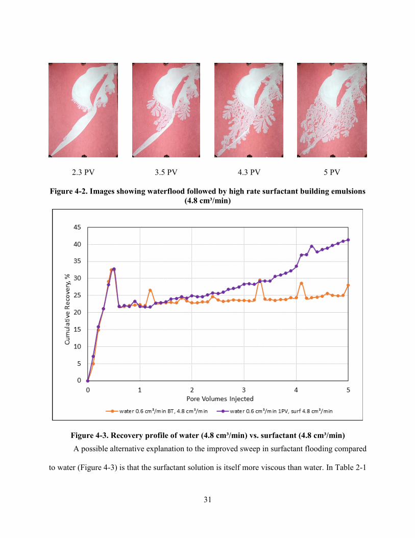
2.3 PV 3.5 PV 4.3 PV 5 PV

Figure 4-2. Images showing waterflood followed by high rate surfactant building emulsions

(4.8 cm³/min)

Figure 4-3. Recovery profile of water (4.8 cm³/min) vs. surfactant (4.8 cm³/min)

A possible alternative explanation to the improved sweep in surfactant flooding compared

to water (Figure 4-3) is that the surfactant solution is itself more viscous than water. In Table 2-1

32

the surfactant solution was measured to have a viscosity of 2.8 mPas, or almost three times the

viscosity of water. In order to know if the improved sweep from the surfactant floods is just due

simply to this higher viscosity of injection fluid, the results are compared against high rate polymer

injection (100 ppm polymer in water). Figure 4-4 shows images of polymer injection at 4.8

cm³/min (shear rate 33.9 s-1) compared to surfactant injection at this same rate. In both polymer

and surfactant flood systems, water was injected (0.6 cm³/min) for 1 PV, and chemical injection

started after that time. While both polymer and surfactant lead to improved sweep compared to

water, the displacement by polymer does not exhibit the high number of small fingers as shown in

the surfactant flood case. Instead, improved sweep by polymer takes the form of several large

fingers that grow and displace continuous heavy oil in the cell.

33

P

S

1 PV 3 PV 4 PV 5 PV

Figure 4-4. Images comparing emulsion sweep to polymer sweep at high injection rate of

4.8 cm³/min

Figure 4-5 compares the recovery profiles for surfactant vs. polymer flooding. Recoveries

are similar for both systems, despite the fact that the bulk polymer solution has a viscosity of close

to 9 mPas at the tested shear rate, compared to just 3 mPas for the surfactant solution. This shows

that the improved surfactant recovery is not just due to its bulk phase viscosity, but rather recovery

and improved sweep results from an effectively higher viscosity emulsion flowing within the Hele-

Shaw cell.

Previous tests in linear core floods (Bryan and Kantzas, 2007; Bryan et al., 2013) discuss

conditions of high shear whereby production fluids are entrained O/W emulsions and water cuts

are consistently still at around 85% or higher. In these conditions, it was previously suggested that

34

rather than plugging water pathways and diverting flow into previously bypassed oil, now O/W

emulsions were forming and being propagated through porous media. In these core floods, this

production of emulsions was accompanied by elevated pressure drop across the core, compared to

the pressure drop from waterflooding. These results, viewed in light of these Hele-Shaw cell

observations, are likely an indication of formation of O/W emulsions that are more viscous than

that of water and so are giving improved sweep even if not complete blockage of water channels.

In the field, complete water channel blockage may not be possible so the process observed in this

study may play a significant role to incremental oil from surfactant flooding in larger 3D systems.

Figure 4-5. Recovery profile of water followed by high rate polymer vs. high rate surfactant

35

CHAPTER 5

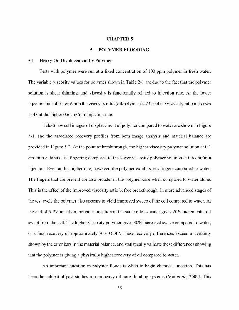
5 POLYMER FLOODING

5.1 Heavy Oil Displacement by Polymer

Tests with polymer were run at a fixed concentration of 100 ppm polymer in fresh water.

The variable viscosity values for polymer shown in Table 2-1 are due to the fact that the polymer

solution is shear thinning, and viscosity is functionally related to injection rate. At the lower

injection rate of 0.1 cm³/min the viscosity ratio (oil/polymer) is 23, and the viscosity ratio increases

to 48 at the higher 0.6 cm³/min injection rate.

Hele-Shaw cell images of displacement of polymer compared to water are shown in Figure

5-1, and the associated recovery profiles from both image analysis and material balance are

provided in Figure 5-2. At the point of breakthrough, the higher viscosity polymer solution at 0.1

cm³/min exhibits less fingering compared to the lower viscosity polymer solution at 0.6 cm³/min

injection. Even at this higher rate, however, the polymer exhibits less fingers compared to water.

The fingers that are present are also broader in the polymer case when compared to water alone.

This is the effect of the improved viscosity ratio before breakthrough. In more advanced stages of

the test cycle the polymer also appears to yield improved sweep of the cell compared to water. At

the end of 5 PV injection, polymer injection at the same rate as water gives 20% incremental oil

swept from the cell. The higher viscosity polymer gives 30% increased sweep compared to water,

or a final recovery of approximately 70% OOIP. These recovery differences exceed uncertainty

shown by the error bars in the material balance, and statistically validate these differences showing

that the polymer is giving a physically higher recovery of oil compared to water.

An important question in polymer floods is when to begin chemical injection. This has

been the subject of past studies run on heavy oil core flooding systems (Mai et al., 2009). This

36

question can be answered for this 2D Hele-Shaw configuration by considering the breakthrough

recovery from polymer vs. water, and the slope of the recovery profile at later times in the flood.

Slopes for these different profiles are depicted in Figure 5-2, and Table 3-1 quantifies the

recoveries and slopes at these various points. The breakthrough oil recovery from water injection

alone at 0.6 cm³/min is 25% OOIP (Table 3-1). Polymer injection at this same rate (viscosity ratio

48) shows very little incremental sweep at the point of breakthrough: 28% OOIP, which is within

the uncertainty of the measurement. When the oil/polymer viscosity ratio is lowered to 23 under

reduced rate of injection, the breakthrough recovery is much higher at 39% OOIP.

In all cases, polymer displacing 1015 mPas oil is an unstable process. The higher viscosity

polymer is able to provide improved recovery at the point of breakthrough, but only when viscosity

is sufficiently high. If not, even with the improved viscosity ratio there is still strong potential for

fingering to develop and recoveries will not be improved significantly compared to water alone.

37

P 0.1

P 0.6

W 0.6

Breakthrough Middle time End of the test

Figure 5-1. Images of polymer flooding (top, middle) and waterflooding (bottom) at

different injection rates.

38

Figure 5-2. Polymer response compared to water

39

Figure 5-3. Waterflood followed by polymer vs. waterflood

The improved response from polymer flooding does not only occur at early times (up to

breakthrough). Figure 5-4 shows that there is also a significant effect of the polymer flood at later

times. Table 5-1 shows that the slope of oil recovery from polymer flooding is around twice the

value of the slope from water injection at the same rate. This means that even after the point of

breakthrough, viscous oil displacement by polymer still has the benefit of the improved viscosity

ratio. In order to test this hypothesis, Figure 5-3 compares the results of straight polymer injection

to the response of a system that is flooded first by water up to 1 PV (i.e. after the point of

breakthrough) and then by polymer at later times. The slope of the oil recovery profile is similar

for the case of continuous polymer vs. polymer after initial water, and both systems show a

recovery slope that is twice the value for water.

40

The results from Figure 5-3 and Figure 5-4 indicate that the value of polymer injection is

not only at early (pre-breakthrough) times but that polymer can also be highly effective at

increasing sweep efficiency with continuous water channels already present across the system.

Table 5-1. Polymer flood summary

Injection rate, cm³/min Polymer 0.1 Polymer 0.6 W 0.3 1 PV, followed by P

0.6

Breakthrough recovery, % 38.77 28.24 24.12

Total recovery at 5 PV Inj, % 68.14 57.65 47.49

RF/PV after 1PV (%OOIP/PV) 5.58 5.59 5.52

Figure 5-4. Comparison of breakthrough and post-breakthrough recovery for

waterflooding and polymerflooding

41

Figure 5-5. Polymer flooding vs. waterflooding followed by polymer flooding

Similar results are observed in polymer floods run after waterflooding in linear heavy oil cores

(Mai et al., 2009; Bryan et al., 2013). The fact that the 2D cell also demonstrates this behavior

(Figure 5-5) means that polymer injection can be started later in the life of a flood and the benefit

of the polymer will still be experienced.

42

CHAPTER 6

6 SURFACTANT-POLYMER FLOODING

6.1 Surfactant-Polymer Injection

While surfactant injection is able to yield incremental oil compared to that of water, field

injection of only surfactant without polymer will be challenging. The emulsions generated in this

system are unstable even at the scale of the Hele-Shaw cell, and in a much larger system it may be

necessary to augment surfactants with polymer to provide stability at the front. 100 ppm polymer

was added to the surfactant solution (15,000 ppm surfactant in water). Table 2-1 lists the viscosity

of the SP solution compared to polymer at various shear rates. At low shear the SP solution is only

60% of the polymer solution viscosity but both polymers and SP solutions are shear thinning so at

the shear rates equivalent to high rate injection the viscosity of polymer and SP solutions are

similar.

When bulk solutions of surfactant and SP were mixed with water (20% oil by mass) both

systems initially formed single phase O/W emulsions. Figure 6-1 shows phase behaviour images

of the surfactant and SP solutions after allowing them to separate for 1 hour and 3 hours,

respectively. After one hour both solutions are still mostly emulsified, but after three hours a

distinct oil/water interface is present for the surfactant solution shown on the left. At this time, oil

is still emulsified in the SP solution on the right. This indicates that interfacial tension is reduced

in the presence of polymer, and in fact with the aqueous phase viscosity higher in this system, the

emulsion separates even more slowly than in the solution with only surfactant added. After 4 hours

the SP solution had separated out and exhibited a clear oil/water interface similar to the surfactant

system.

43

Time = 0

After 3 hours

Figure 6-1. Images of surfactant vs. SP bottle test

Figure 6-2 shows the Hele-Shaw cell images taken at the same time for SP and surfactant

systems. For the same injection volume, it is clear that the sweep efficiency of the SP solution is

greater than that of the surfactant system alone. What is perhaps unexpected is that the images of

SP displacement still show the presence of many small viscous fingers that have moved away from

44

the pre-formed water channels and into bypassed oil. The viscosity of the SP solution is basically

the same as for the polymer that was flooded in Figure 4-5. In the polymer flood, displacement

occurs in the form of broad water fingers that extend through the model. With surfactant added to

the polymer, the presence of fingers indicates that the formation and flow of O/W emulsions is

still happening. Adding polymer assists in raising the overall viscosity of the solution, but the

surfactant’s effect of generating and flowing more viscous emulsions is still present. As with the

case of surfactant alone, the effect of these emulsions is to push away from the pre-formed water

pathways and give improved areal sweep efficiency of the viscous oil.

SP

S

1.5 PV 2.5 PV 3.5 PV 4.5 PV

Figure 6-2. Images of water followed by high rate surfactant and SP solution

45

Figure 6-3 plots the oil recovery profile for SP injection compared to high rate surfactant

alone and to water. The combination of surfactant and polymer clearly leads to a better recovery

than surfactant injection alone. Moreover, it is not just the effect of the polymer viscosity

responsible for this improvement, since polymer alone recovery is similar to the surfactant flood

alone (Figure 4-5). Instead, there is a clear synergy between the two chemicals: polymer stabilizes

the displacement front and improves production of oil, and surfactant addition leads to the flow of

O/W emulsions that are less mobile than just the aqueous phase alone. The reason for oil

displacement is improved sweep efficiency: water channels are not being blocked off like in a

linear core, but instead the impact of emulsions is to reduce water/polymer mobility further giving

a higher overall contact within the Hele-Shaw cell.

46

Figure 6-3. Recovery profile of water and high rate surfactant vs. water and high rate SP

47

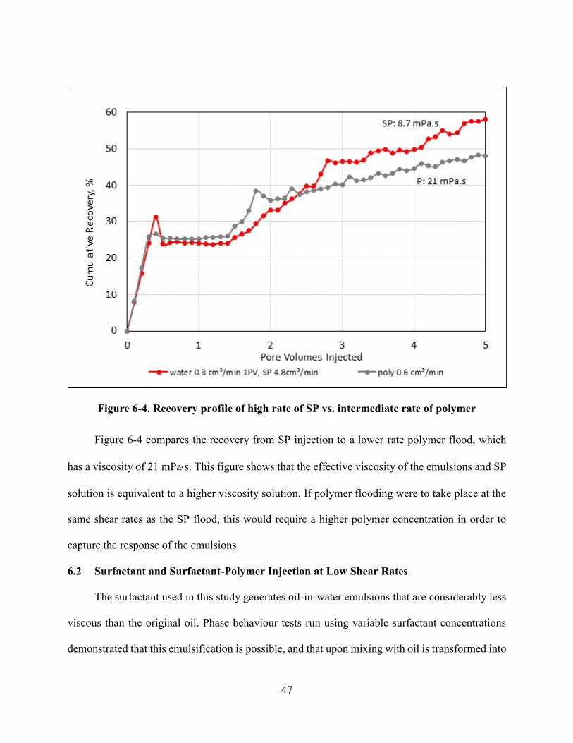
Figure 6-4. Recovery profile of high rate of SP vs. intermediate rate of polymer

Figure 6-4 compares the recovery from SP injection to a lower rate polymer flood, which

has a viscosity of 21 mPas. This figure shows that the effective viscosity of the emulsions and SP

solution is equivalent to a higher viscosity solution. If polymer flooding were to take place at the

same shear rates as the SP flood, this would require a higher polymer concentration in order to

capture the response of the emulsions.

6.2 Surfactant and Surfactant-Polymer Injection at Low Shear Rates

The surfactant used in this study generates oil-in-water emulsions that are considerably less

viscous than the original oil. Phase behaviour tests run using variable surfactant concentrations

demonstrated that this emulsification is possible, and that upon mixing with oil is transformed into

48

a low viscosity emulsion. The presence of emulsification is evidence that oil/water interfacial

tension has been reduced, and the fact that separation occurs in the space of hours means that

interfacial tension is not at ultra-low levels that would cause stable emulsions to form. Phase

separation was slowest with 15,000 ppm surfactant and therefore this is the concentration that was

applied in all the Hele-Shaw floods.

Figure 6-5 shows Hele-Shaw cell images taken at various stages throughout the surfactant

flood. The top row of images is surfactant flooding, and waterflooding (the bottom row) shows the

same rate. Clearly with the addition of surfactant, the degree of fingering actually increases

throughout the system. Instability analysis (Bentsen, 1985) confirms this observation: under

adverse mobility ratio the injection fluid will tend to finger through the oil, and interfacial tension

helps to offset this fingering by minimizing the total contact area between oil and injection fluid.

With surfactant present, this force to offset pre-breakthrough viscous fingering is no longer present

and the amount of fingering is much higher than for water injection alone. Recovery profiles are

plotted in Figure 6-6 and Table 6-1 documents the breakthrough recovery for surfactant injection

at 0.6 cm³/min. The breakthrough recovery occurs at only 12% OOIP, or half the breakthrough

recovery from water (Figure 6-6). At low injection rates there is insufficient shear applied to

emulsify oil into water, so what is shown is just the effect of reduced interfacial tension. On this

basis alone, surfactant leads to a reduced recovery at breakthrough compared to water. This is

despite the fact that the surfactant solution is already more viscous than water alone, so the

viscosity ratio is already improved to 282. Similar to what was observed in the polymer flood at

0.6 cm³/min, the impact of viscosity ratio at this level does not improve pre-breakthrough recovery

so the negative effect of fingering dominates during this time.

49

S 0.6

SP 0.6

W 0.6

1.5 PV 2.5 PV 3 PV 5 PV

Figure 6-5. Images of surfactant and SP injection at 0.6 cm³/min

50

W 0.6 S 0.6

Figure 6-6. Images taken at breakthrough during waterflooding and surfactant flooding at

0.6 cm³/min

The benefit of surfactant flooding comes during the post-breakthrough flood response.

With such a high degree of fingering present, overall the region swept by water/chemical is higher

than that of water alone (Figure 6-5 and Figure 6-6). The slope of the oil recovery curve at later

times is 5.8 % OOIP/PV injected, or 2.6 times the slope of the recovery profile from water

injection.

Further insight into the surfactant recovery process comes from observation of the nature

of the images in Figure 6-5: by the end of the flood the images appear to have a high degree of

sweep across the cell while the material balance recovery is only 50%. Clearly the swept regions

within the Hele-Shaw cell still contain a lot of oil, so it would be incorrect to assume that all regions

swept correspond to oil recovery. In order to compare the image analysis to the actual material

balance recovery, the image thresholding had to be changed to exclude this swept region from the

predicted recovery. At the inlet end of the cell, continued surfactant injection cleaned all the oil

off the glass and the region that is swept completely of oil continues to grow with time.

Furthermore, the region apparently swept by surfactant (top row of Figure 6-5) is approximately

51

the same size in all images, even though oil recovery increases with time. In this system, the

mechanism of oil recovery is represented by chemical solution fingering through the oil and then

continuously flowing along the same pathways, stripping more oil from these channels due to

reduced interfacial tension and mixing between oil and water phases.

Figure 6-6 also compares the polymer flooding recovery profile at this same rate to the

response from water and surfactant testing. Despite the improved viscosity ratio from polymer

flooding, the slope of the recovery profile is similar to that of the surfactant flood. This means that

the efficiency from the viscosity ratio improvement is similar to the process of oil mixing with

water and flowing along the water channels.

Figure 6-7. Low rate injection (0.6 cm³/min) of surfactant, polymer and water

52

The overall higher recovery from the polymer compared to surfactant flooding is due to

the low breakthrough recovery from the surfactant flood. The more viscous polymer solution is

important for providing improved sweep at early times, and even at later times an improved

viscosity ratio is able to give a similar response compared to the surfactant alone. In a viscous oil

system, the improved viscosity ratio resulting from polymer injection can be an important process

aid.

A surfactant-polymer (SP) solution was therefore generated, consisting of the same 15,000

ppm surfactant and 100 ppm polymer that was used in each system by itself. Table 2-1 shows that

the viscosity of the SP solution is lower than that of the polymer alone, but at higher rates (4.8

cm³/min) this difference becomes insignificant. Phase behaviour tests confirmed that the addition

of polymer does not adversely affect the ability of the surfactant to emulsify oil. An SP flood was

run at the same injection rate (0.6 cm³/min) and Figure 6-8 plots the recovery profile from SP

flooding compared to polymer flooding alone. Results are quantified in Table 6-1; in this test the

first 1 PV injected fluid is water, and chemical (polymer or SP) is subsequently run.

Despite the fact that the viscosity ratio is worse for SP injection compared to polymer, the

recovery is much higher for the SP system. In fact, the recovery at 5 PV injection is 17% higher

for SP injection than for polymer alone. The slope of the SP recovery profile is 9.7 % OOIP/PV

injected, which is 4.3 times more than the slope for waterflooding and 1.7 times more than the

slope from polymer or surfactant injection alone. The mechanism by which the SP flood works is

understood by observing the Hele-Shaw cell images in Figure 6-5. When water is switched to SP

injection, this more viscous fluid leads to generation of fingers that move away from the existing

water channels to access new areas of the cell. This new invaded area is swept by the more viscous

SP solution and therefore the higher degree of fingering from the surfactant is still visible, but

53

overall the degree of sweep in the chemical contacted area is enhanced by the presence of polymer.

When comparing the swept regions resulting from surfactant vs. SP injection, it is clear that in all

regions contacted by chemical, the SP solution has provided a better sweep than the more gradual

stripping observed during surfactant flooding alone. Figure 6-9 confirms previous statement for

SP system based on recovery at the breakthrough and after the breakthrough.

Figure 6-8. Water followed by polymer vs. water flowed by SP

54

Table 6-1. Low rate surfactant and SP injection summary

Injection rate, cm³/min S 0.6 W 0.3 1 PV, followed by SP 0.6

Breakthrough recovery, % 12.24 24.51

Total recovery at 5 PV Inj, % 50.20 64.46

RF/PV after 1PV (% OOIP/PV) 5.81 9.67

Figure 6-9. Water, surfactant, polymer and SP at lower shear rates

6.3 Surfactant and Surfactant-Polymer Injection at High Shear Rates

Phase behaviour tests of oil and surfactant solutions verified that the surfactant is able to

emulsify oil into water and effectively convert the viscous oil into a mobile emulsion phase.

However, produced fluids from the low rate surfactant test did not show evidence of produced

emulsions. A set of additional tests were therefore run at much higher injection rates of 4.8 cm³/min

with the goal of providing more shear to the displacement enhancing formation and flow of

emulsions within the cell.

Figure 6-10 shows Hele-Shaw cell images of high rate surfactant flooding compared to the

previous lower injection at 0.6 cm³/min. In the high rate flood, the procedure applied was to inject

55

surfactant at 0.6 cm³/min until breakthrough, and then increase injection rates. The rest of the flood

(up to 5 PV injection) was run at 4.8 cm³/min. At the point of breakthrough, both the high rate and

low rate surfactant systems had been initially flooded at the same rate (0.6 cm³/min) so

breakthrough recovery is very similar in both systems. At later times in the flood, the high rate

injection does not appear to give as much sweep as the surfactant at 0.6 cm³/min but the actual

recovery profile shown in Figure 6-11 is similar for both surfactant systems. This further

corroborates the previous observation that in the low rate surfactant flood, with oil swept along the

moving water channels, the visibly swept area still contains significant remaining oil saturation.

In contrast, during high rate surfactant injection the area that was swept is free of oil, and the

normal thresholding image analysis technique can be applied to predict recovery similar to

polymer or waterflooding.

Previous observation showed that in the case of low rate surfactant flooding (0.6 cm³/min)

the area swept by chemical does not appear to change much with time. Oil recovery mechanism at

these low rates is stripping off oil along preformed water channels. In the high rate flood (4.8

cm³/min) test, the nature of the recovery is quite different: here the system initially contains many

small fingers but one major pathway traversing the cell. Under high injection rate of surfactant,

the swept area increases with time. This means that the surfactant mixes with water to form in-situ

emulsions which act to block off current fingers and force flow into previously unswept regions

of the cell. The recovery from high rate chemical flooding is similar to that of polymer injection

after waterflooding: the mobility ratio changes between oil and the injection fluid, and resulting in

improved sweep efficiency of the cell. Water channel blockage and flow re-diversion have

previously been proposed as mechanisms for surfactant-based heavy oil recovery (Bryan and

Kantzas, 2009) but these were observed in linear core flood tests. It is significant that similar

56

observations are made from this 2D cell that does not allow for pore-scale blockage of water

channels.

S 0.6

SP 0.6

W 0.6

1.5 PV 2.5 PV 3 PV 5 PV

Figure 6-10. Images of surfactant, surfactant-polymer and water injection at 0.6 cm³/min

57

Another possible explanation for the enhanced sweep efficiency mechanism observed at

high rates is that with such fast injection into a viscous oil system, the build-up of pressure across

the core is responsible for the improved oil recovery response. In order to test this assumption,

Figure 6-9 also shows the response for a high rate waterflood: here water was injected at 0.6

cm³/min up to the point of breakthrough, and then chemical-free water was flushed through the

core at 4.8 cm³/min. Despite the build-up of pressure gradients that could have occurred for this

high rate waterflood, Figure 6-9 shows that high rate water injection leads to no incremental oil

recovery after point of breakthrough. Instead, water flowed only through its preformed channels

and there was no additional water finger snap-off with associated sweep area increases which

occurred previously at low rates. Therefore, the surfactant is responsible for incremental oil

recovery under high injection rates: it is the formation of in-situ emulsions that re-divert flow, not

just the buildup of pressure across the cell.

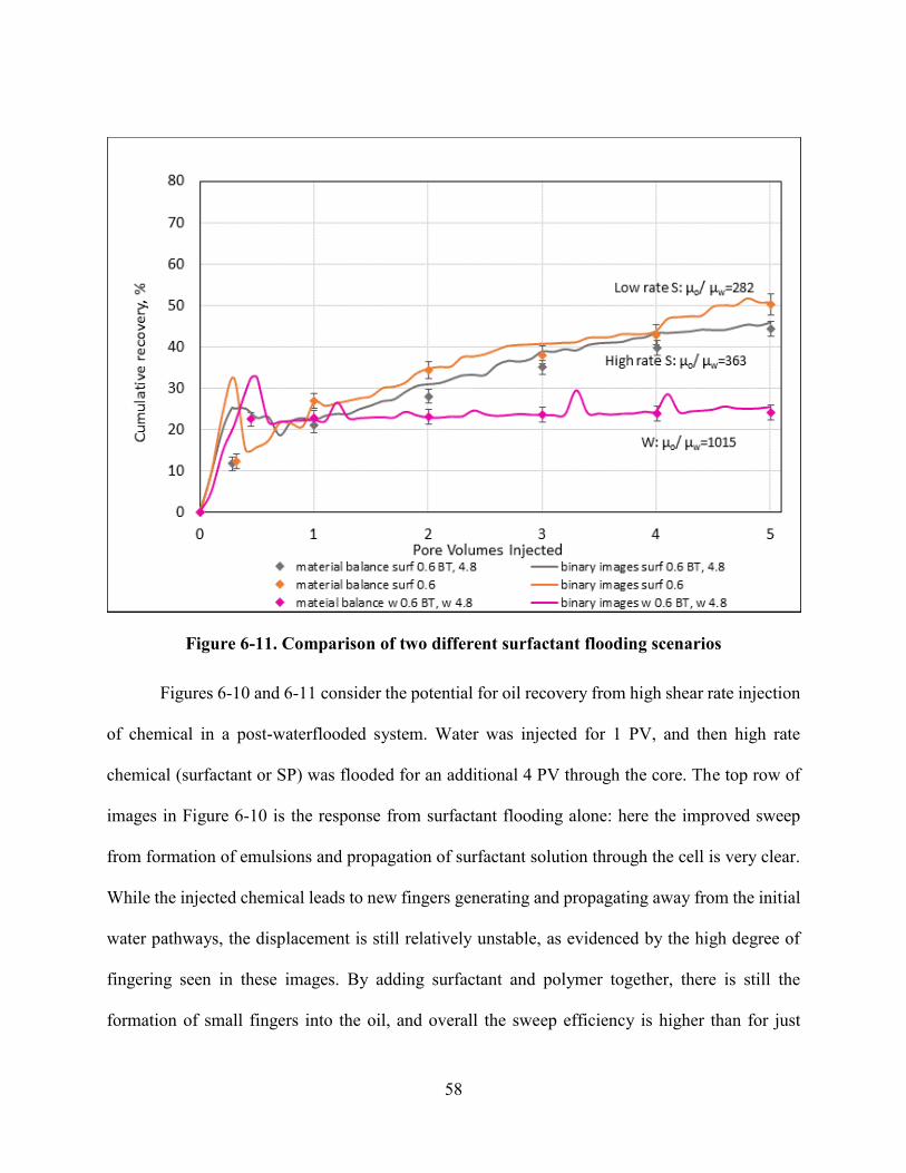
58

Figure 6-11. Comparison of two different surfactant flooding scenarios

Figures 6-10 and 6-11 consider the potential for oil recovery from high shear rate injection

of chemical in a post-waterflooded system. Water was injected for 1 PV, and then high rate

chemical (surfactant or SP) was flooded for an additional 4 PV through the core. The top row of

images in Figure 6-10 is the response from surfactant flooding alone: here the improved sweep

from formation of emulsions and propagation of surfactant solution through the cell is very clear.

While the injected chemical leads to new fingers generating and propagating away from the initial

water pathways, the displacement is still relatively unstable, as evidenced by the high degree of

fingering seen in these images. By adding surfactant and polymer together, there is still the

formation of small fingers into the oil, and overall the sweep efficiency is higher than for just

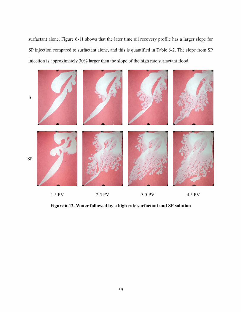
59

surfactant alone. Figure 6-11 shows that the later time oil recovery profile has a larger slope for

SP injection compared to surfactant alone, and this is quantified in Table 6-2. The slope from SP

injection is approximately 30% larger than the slope of the high rate surfactant flood.

S

SP

1.5 PV 2.5 PV 3.5 PV 4.5 PV

Figure 6-12. Water followed by a high rate surfactant and SP solution

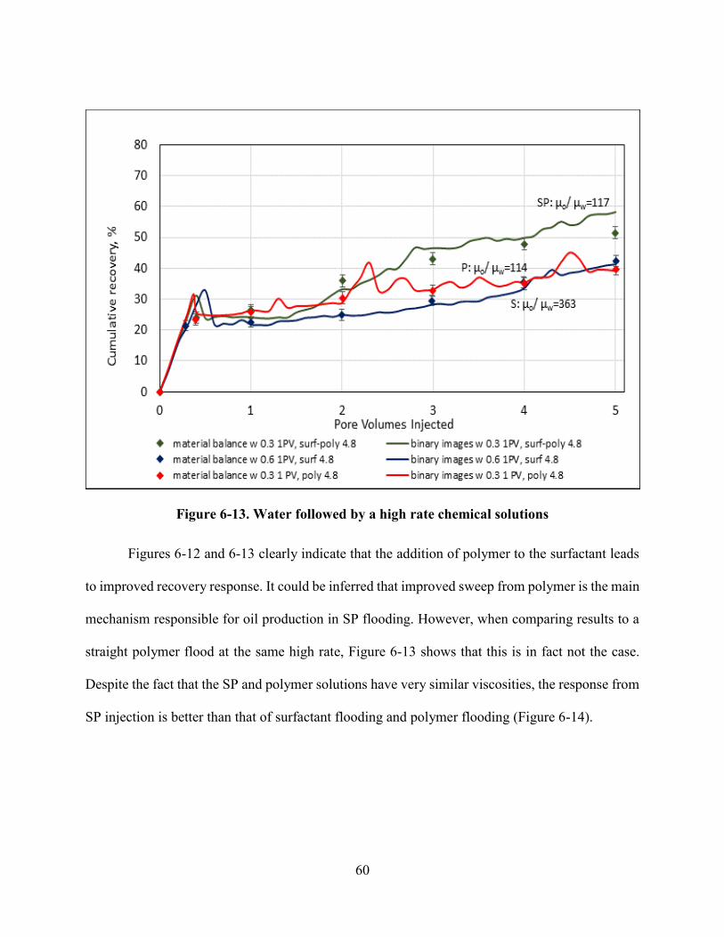
60

Figure 6-13. Water followed by a high rate chemical solutions

Figures 6-12 and 6-13 clearly indicate that the addition of polymer to the surfactant leads

to improved recovery response. It could be inferred that improved sweep from polymer is the main

mechanism responsible for oil production in SP flooding. However, when comparing results to a

straight polymer flood at the same high rate, Figure 6-13 shows that this is in fact not the case.

Despite the fact that the SP and polymer solutions have very similar viscosities, the response from

SP injection is better than that of surfactant flooding and polymer flooding (Figure 6-14).

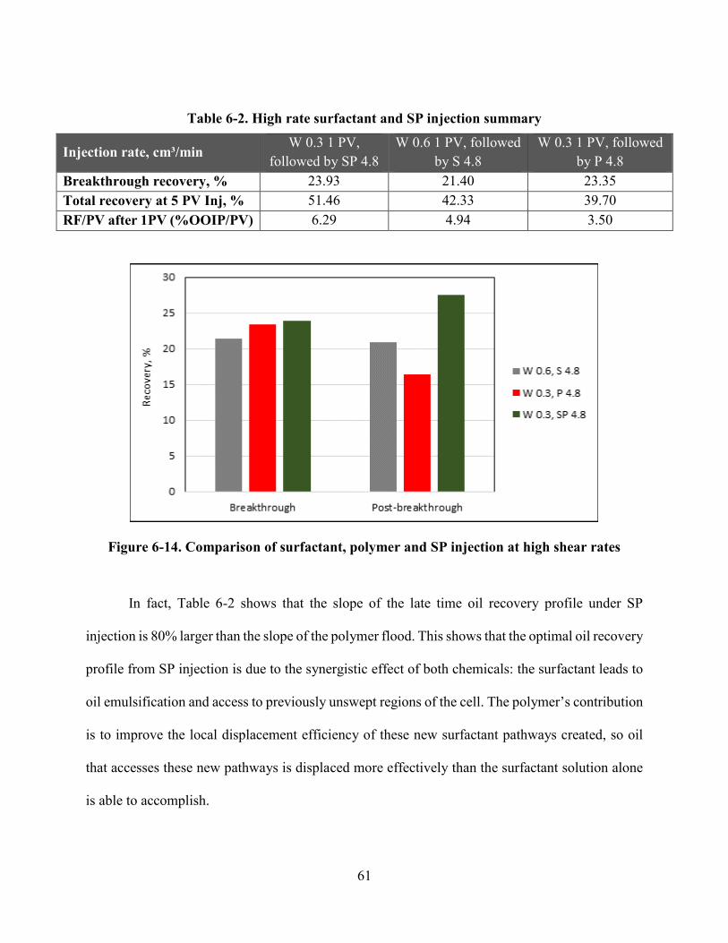
61

Table 6-2. High rate surfactant and SP injection summary

Injection rate, cm³/min W 0.3 1 PV,

followed by SP 4.8

W 0.6 1 PV, followed

by S 4.8

W 0.3 1 PV, followed

by P 4.8

Breakthrough recovery, % 23.93 21.40 23.35

Total recovery at 5 PV Inj, % 51.46 42.33 39.70

RF/PV after 1PV (%OOIP/PV) 6.29 4.94 3.50

Figure 6-14. Comparison of surfactant, polymer and SP injection at high shear rates

In fact, Table 6-2 shows that the slope of the late time oil recovery profile under SP

injection is 80% larger than the slope of the polymer flood. This shows that the optimal oil recovery

profile from SP injection is due to the synergistic effect of both chemicals: the surfactant leads to

oil emulsification and access to previously unswept regions of the cell. The polymer’s contribution

is to improve the local displacement efficiency of these new surfactant pathways created, so oil

that accesses these new pathways is displaced more effectively than the surfactant solution alone

is able to accomplish.

62

CHAPTER 7

7 CONCLUSIONS

The tests run in this study demonstrate recovery mechanisms and sweep efficiency in a 2D

system with no local pore scale plugging of water channels. The major finding of this work is that

heavy oil recovery is improved by chemical injection, so results are not a laboratory artifact from

linear core floods. In particular, several production mechanisms are observed from these Hele-

Shaw tests:

Even without plugging of water channels and re-diversion of fluids as is seen in core floods,

surfactant injection can still lead to improved oil recovery compared to waterflooding. The

addition of surfactant and shear leads to the generation of O/W emulsions, which exist as

fingers propagating away from the previously swept water zones. In this manner, surfactant

leads to improved sweep similar to a polymer flood.

Polymer injection leads to improved sweep compared to water. This improved sweep is

not only present as reduced fingering prior to breakthrough, but it is also present at late

times in the polymer flood. In fact, the slope of oil recovery from polymer is similar for

either direct polymer injection or polymer flooding after water, so polymer flooding can

successfully be implemented into previous waterflooded zones with the same expected

effectiveness as for direct polymer injection.

Low rate surfactant flooding works by reducing interfacial tension between oil and water

and leading to the creation of many small fingers of water penetrating through the oil.

While this leads to early water breakthrough, at later times in the flood the surfactant

solution allows oil to partially mix with water and drags this mobilized oil along the

preformed sweep pathways towards the exit of the cell.

63

High rate surfactant injection works by generating oil-in-water emulsions and injection

fingers that move away from water channels into previously unswept regions of the cell.

Within the reservoir, where shear forces are higher than found in this 2D cell, this may be

the dominant recovery mechanism from surfactant flooding. The result is that high rate

surfactant floods yield incremental oil in a similar fashion to polymer floods.

The addition of surfactant and polymer together lead to an optimized oil recovery response

that is better than response achieved for either polymer or surfactant injection alone. The

effect of the surfactant is to generate emulsions and fingers away from water pathways and

into previously unswept oil, and when this happens the polymer allows more effective

displacement of this new oil than by surfactant alone.

It should be emphasized that the recoveries and sweep efficiencies presented in this work are

not necessarily reflective of oil recovery in porous media. The goal of the Hele-Shaw tests was to

conduct floods in a system with no local pore-level trapping of fluids, and with the enhanced flow

effects of a linear core flood eliminated. These tests are designed to provide a mechanistic

understanding of heavy oil recovery mechanisms by surfactant and polymer systems. Conducting

micromodel experiments is a complementary option to confirm the obtained results and achieve

more realistic displacement patterns in porous media.

64

REFERENCES

Alvarado, D. A., and Marsden, S. S. 1979. Flow of Oil-in-Water Emulsions Through Tubes and

Porous Media. Society of Petroleum Engineers. doi:10.2118/5859-PA.

Alvarez, J. M., and Sawatzky, R. P. 2013. Waterflooding: Same Old, Same Old? Society of

Petroleum Engineers. doi:10.2118/165406-MS.

Asghari, K., and Nakutnyy, P. 2008. Experimental Results of Polymer Flooding of Heavy Oil

Reservoirs. Petroleum Society of Canada. doi:10.2118/2008-189.

Beliveau, D. 2009. Waterflooding Viscous Oil Reservoirs. Society of Petroleum Engineers.

doi:10.2118/113132-PA

Bentsen, R. G. 1985. A New Approach to Instability Theory in Porous Media. Society of

Petroleum Engineers. doi:10.2118/12725-PA.

Brock, D. C., and Orr, F. M. 1991. Flow Visualization of Viscous Fingering in Heterogeneous

Porous Media. Society of Petroleum Engineers. doi:10.2118/22614-MS.

Bryan, J. and Kantzas, A., 2009. Potential for alkali-surfactant flooding in heavy oil reservoirs

through oil-in-water emulsification. Journal of Canadian Petroleum Technology, 48(02),

pp.37-46.

Bryan, J. L., and Kantzas, A. 2007. Enhanced Heavy-Oil Recovery by Alkali-Surfactant Flooding.

Society of Petroleum Engineers. doi:10.2118/110738-MS.

Bryan, J. L., Shamekhi, H., Su, S., Kantzas, A. 2013. Insights into Heavy Oil Recovery by

Surfactant, Polymer and ASP Flooding. Society of Petroleum Engineers. doi:10.2118/165440-

MS.

65

Bryan, J.L. and Kantzas, A., 2008, January. Improved recovery potential in mature heavy oil fields

by alkali-surfactant flooding. In International Thermal Operations and Heavy Oil Symposium.

Society of Petroleum Engineers.

Buckley, S. E., and Leverett, M. C. 1942. Mechanism of Fluid Displacement in Sands. Society of

Petroleum Engineers. doi:10.2118/942107-G.

Chatenever, A. and Calhoun, J.C. 1952. Visual Examinations of Fluid Behavior in Porous Media.1.

Transactions of the American Institute of Mining and Metallurgical Engineers 195, 149-156.

Coskuner, G., and Bentsen, R. G. 1988. A Hele-Shaw Cell Study of a New Approach to Instability

Theory In Porous Media. Petroleum Society of Canada. doi:10.2118/88-01-09.

Delamaide, E., Zaitoun, A., Renard, G., and Tabary, R. 2013. Pelican Lake Field: First Successful

Application of Polymer Flooding in a Heavy Oil Reservoir. Society of Petroleum Engineers.

doi:10.2118/165234-MS.

Dusseault, M.B., 2002. CHOPS: Cold Heavy Oil Production with Sand in the Canadian heavy oil

industry. Alberta Department of Energy.

Engelberts, W. F., and Klinkenberg, L. J. 1951. Laboratory Experiments on the Displacement of

Oil by Water from Packs of Granular Material. World Petroleum Congress.

Green, D.W., Willhite G.P., Enhanced Oil Recovery, 978-1-55563-077-5SPE Publications, 1998.

Hassan Z. Harraz, World Petroleum Resources, Presentation, 2016.

Hill, J. Laboratory Manual for Engineering Thermodynamics. 2012. University of Calgary,

Calgary, AB.

Hornof, V., and Morrow, N. R. 1988. Flow Visualization of the Effects of Interfacial Tension on

Displacement. Society of Petroleum Engineers. doi:10.2118/14930-PA.

66

Hou, J.R., Liu, Z.C., Dong, M.Z., Yue, X.A. and Yang, J.Z. 2006. Effect of viscosity of

alkaline/surfactant/polymer (ASP) solution on enhanced oil recovery in heterogeneous

reservoirs. Journal of Canadian Petroleum Technology 45(11), 27-33.

Huang, S. and Dong, M. 2004. Alkaline/surfactant/polymer (ASP) flood potential in southwest

Saskatchewan oil reservoirs. Journal of Canadian Petroleum Technology 43(12), 56-61.

Hunky, R. M., Wu, Y., Bai, B., and Dunn-Norman, S. 2010. An Experimental Study of Alkaline

Surfactant Flooding for Ultra Shallow Heavy Oil Reservoirs. Society of Petroleum Engineers.

doi:10.2118/132537-MS

International Energy Agency. 2004. World Energy Outlook.

Jardine, D. "Cretaceous oil sands of western Canada." 1974. pp. 50-67.

Kumar, M., Hoang, V. T., and Satik, C. 2005. High Mobility Ratio Water Flood Performance

Prediction: Challenges and New Insights. Society of Petroleum Engineers. doi:10.2118/97671-

MS.

Kumar, R., and Mohanty, K. K. 2011. Sweep Efficiency of Heavy Oil Recovery by Chemical

Methods. Society of Petroleum Engineers. doi:10.2118/146839-MS

Liu, Q., Dong, M., and Ma, S. 2006. Alkaline/Surfactant Flood Potential in Western Canadian

Heavy Oil Reservoirs. Society of Petroleum Engineers. doi:10.2118/99791-MS.

Mai, A. and Kantzas, A. 2009. Heavy oil waterflooding: effects of flow rate and oil

viscosity. Journal of Canadian Petroleum Technology, 48(03), pp.42-51.

Mai, A., and Kantzas, A. 2008. Mechanisms of Heavy Oil Recovery by Low Rate Waterflooding.

Petroleum Society of Canada. doi:10.2118/2008-156.

Mai, A., Bryan, J., Goodarzi, N., and Kantzas, A. 2009. Insights Into Non-Thermal Recovery of

Heavy Oil. Petroleum Society of Canada. doi:10.2118/09-03-27.

67

Miller, K. A. 2006. Improving the State of the Art of Western Canadian Heavy Oil Waterflood

Technology. Petroleum Society of Canada. doi:10.2118/06-04-GE

Oilfield Review, Winter 2010/2011: Volume 22, no.4, Schlumberger.

Pei, H., Zhang, G., Ge, J., Tang, M. and Zheng, Y. 2012. Comparative effectiveness of alkaline

flooding and alkaline–surfactant flooding for improved heavy-oil recovery. Energy and Fuels,

26(5), pp.2911-2919.

Saffman, P.G. and Taylor, G. 1958. The Penetration of a Fluid into a Porous Medium or Hele-

Shaw Cell Containing a More Viscous Liquid. Proceedings of the Royal Society of London

Series a-Mathematical and Physical Sciences 245(1242), 312-319.

Santanna, V.C., Curbelo, F.D.S., Dantas, T.N.C., Neto, A.A.D., Albuquerque, H.S. and Garnica,

A.I.C. 2009. Microemulsion flooding for enhanced oil recovery. Journal of Petroleum Science

and Engineering 66(3-4), 117-120.

Sedaghat, M., Mohammadzadeh, O., Kord, S., and Chatzis, I. 2015. Pore-Level Experimental

Investigation of ASP Flooding to Recover Heavy Oil in Fractured Five-Spot Micromodels.

Society of Petroleum Engineers. doi:10.2118/174290-MS

Seright, R. (2010, August 1). Potential for Polymer Flooding Reservoirs With Viscous Oils.

Society of Petroleum Engineers. doi:10.2118/129899-PA.

Sheng, J.J. 2011. Modern Chemical Enhanced Oil Recovery-Theory and Practice, GPP, pp. 13-

181.

Sim, S. S.-K., Wassmuth, F. R., and Bai, J. J. 2014. Identification of Winsor Type III Micro-

emulsion for Chemical EOR of Heavy Oil. Society of Petroleum Engineers.

doi:10.2118/170018-MS.

68

Smith, G. E. 1992. Waterflooding Heavy Oils. Society of Petroleum Engineers.

doi:10.2118/24367-MS.

Van Meurs, P. 1957. The Use of Transparent Three-Dimensional Models for Studying the

Mechanism of Flow Processes in Oil Reservoirs. Society of Petroleum Engineers.

Vittoratos, E., West, C.C. and Black, C.J. 2007. Flow Regimes of Heavy Oils Under Water

Displacement. EAGE 14th European IOR, April, pp.22-24.

Voroniak, A., Bryan, J. L., Hejazi, H., and Kantzas, A. 2016. Two-Dimensional Visualization of

Heavy Oil Displacement Mechanism During Chemical Flooding. Society of Petroleum

Engineers. doi:10.2118/181640-MS.

Voroniak, A., Bryan, J. L., Taheri, S., Hejazi, H., and Kantzas, A. 2016. Investigation of Post-

Breakthrough Heavy Oil Recovery by Water and Chemical Additives Using Hele-Shaw Cell.

Society of Petroleum Engineers. doi:10.2118/181149-MS.

Wang, J., and Dong, M. 2007. A Laboratory Study of Polymer Flooding for Improving Heavy Oil

Recovery. Petroleum Society of Canada. doi:10.2118/2007-178.

Wassmuth, F. R., Green, K., and Bai, J. 2012. Associative Polymers Outperform Regular Polymers

Displacing Heavy Oil in Heterogeneous Systems. Society of Petroleum Engineers.

doi:10.2118/157916-MS.

Wassmuth, F. R., Green, K., Arnold, W., and Cameron, N. 2009. Polymer Flood Application to

Improve Heavy Oil Recovery at East Bodo. Petroleum Society of Canada. doi:10.2118/09-02-

558.

Winsor, P.A. 1948. Hydrotropy, solubilisation and related emulsification processes. Transactions

of the Faraday Society 44(0), 376-398.

69

Wooding, R.A. 1960. Instability of a Viscous Liquid of Variable Density in a Vertical Hele-Shaw

Cell. Journal of Fluid Mechanics 7(4), 501-515.

Xianli, K., Haghighi, M., and Yortsos, Y. C. 1992. Visualization experiments on steam injection

in Hele-Shaw cells. No. DOE/BC/14600--20. University of Southern California, Los Angeles,

CA (United States). Dept. of Chemical Engineering.

70

APPENDIX A: RHEOLOGICAL PROPERTIES OF CHEMICAL SOLUTIONS

For given flow rates:

Q1 = 0.1 cm³/min

Q2 = 0.6 cm³/min

Q3 = 4.8 cm³/min

Corresponding shear rates:

ϒ1 = 0.72 1/s

ϒ2 = 4.24 1/s

ϒ3 = 33.90 1/s

Figure A-1. Surfactant viscosity vs. shear rate

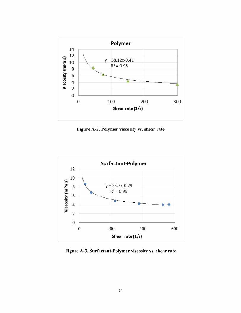
71

Figure A-2. Polymer viscosity vs. shear rate

Figure A-3. Surfactant-Polymer viscosity vs. shear rate

72

APPENDIX B: COPYRIGHT PERMISSION LETTERS

73