visual pattern recognition and learning - computer science

V. Wojcik + P. Comte: October 2009 Speedy Visual Inspection of Retinal Images v.20P - of 32

Algorithms for Speedy Visual Recognition and Classification of Patterns Formed on Rectangular Imaging Sensors

Vlad Wojcik and Pascal Comte

Department of Computer Science Brock University

October 2009

ABSTRACT:

We present a survey of conceptual and technological challenges facing the computer vision practitioners. The real-time tasks of image interpretation, pattern clustering, recognition and classification necessitate quick analysis of registered patterns. Current algorithms and technological approaches are slow and rigid. Within the evolutionary context, having performed the simulation of human visual cortex, we present a novel, biologically inspired solution to these problems, with aim to accelerate processing. Our massively parallel algorithms are applicable to patterns recorded on rectangular imaging arrays of arbitrary sizes and resolutions. The systems we propose are capable of continuous learning, as well as of selective forgetting less important facts, and so to maintain their adaptation to an environment evolving sufficiently slowly. A case study of visual signature recognition illustrates the presented ideas and concepts.

1. Our conceptual and technological challenges The problem of scanning semiconductor CCD sensors is relevant to larger efforts of creation of artificial brains on a number of levels: First: The imaging sensors can be seen as silicon retinas of an artificial brain. In a biological, mammalian system the retina is a part of the brain; indeed, it is the only externally visible (upon careful but non-invasive inspection) part of the central nervous system (CNS) of any mammal. Second: Human visual experience tells us that biological image processing is a multi-layer computation with some of the processing happening at the conscious and unconscious levels. For example: our visual experience leaves us completely unaware of the fact that the images formed on our retinas are granular, i.e. made of "pixels" associated with excitation of sensors (rods and cones). On the other hand, we have conscious access to pre-processed images, which we try to understand. While computerized image understanding is advancing in strides, it is hampered by the fact that we still do not know how to make a machine pay selective attention to "important" regions of an image,


while treating other regions as less relevant. In this paper we argue that paying attention amounts to allocation of computing power, and we offer insights as to how make a machine achieve this feat. Third: Most implementations of artificial brains rely on artificial neural networks (ANN). Much progress is being made in constructing ANNs geared towards particular tasks. However, the ANN methodology yields black box systems, i.e. systems that work, but still leaves us in the dark why they work. While this approach is undeniably useful (for example: we routinely take medicines that work while not knowing why they work), it prevents us from gaining deeper understanding of the systems we have successfully modeled. Most of us construct artificial brains in order to gain deeper insight into the inner functionality of a biological brain. It is not at all clear to us (authors) that ANNs offer the simplest path to gain such knowledge. In contrast, the methodology we present leads to creation of white box models, leaving us in full understanding of the functionality of our models. We treat ANNs as one possible technology for implementation of white boxes, artificial brains, etc. Fourth: If we do not understand why the device works, we find it exceedingly difficult to improve it. We have no choice but to abandon the old device and construct and train the new and improved device from scratch. Evolution seems to work in this way. The black box ANN methodology offers the case in point: We have difficulties in expanding functionality of ANNs previously constructed, while preserving their old knowledge. Mysteriously, this stands in stark contrast to biological systems that are capable of continuous learning. Facing these conceptual challenges we present an approach overcoming these difficulties. Our trained white box systems are capable of continuous learning. Additionally, the knowledge they acquire is as valuable as the systems themselves and can be shared with other, newer systems occupying the same application niche. As if the above conceptual challenges were not enough, we face a number of technological obstacles too: Real-time robotic understanding of perceived images is exceedingly challenging and demands high computing power and novel parallel algorithms. The processing power available today is woefully scarce. As a case in point consider the speed of leading professional cameras offered currently by market leaders: Nikon and Canon. The film camera model Nikon F6, capable of shooting 8 frames per second, may be compared to its digital counterpart, model D3x, which offers the resolution of 24 megapixels, and shoots at 5 fps rate [1]. (Faster shooting rates are available in the resolution crop mode) Interestingly, if we scan a single full frame of the old 35 mm film with Microtek ArtixScan M1 scanner at 4800 ppi resolution we can obtain a 36-megapixel image [2]. Canon cameras fare no better: The top film model EOS-1v is capable of shooting at 10 fps, while its digital counterpart EOS-1Ds Mark III (a dual-processor, 21 megapixel camera) features the shooting rate of up to 5 fps [3]. Using that scanner a 6x7 cm medium format film frame yields 130 megapixel scan of astounding quality, which, when saved, produces a 400 MB TIFF file. Note that this resolution is roughly equivalent to that of the human retina. Scanners offering higher resolutions exist. The challenge is to process such images in real time, to offer digital IMAX 3D cinema first, and real-time adaptive


3D robotic vision later. Construction of a robot with an artificial brain and visual acuity comparable to human lays in more distant future. Typically mechanical devices are slower when compared to electronic devices, which do not have moving parts. Yet in the previous examples, the mechanical still film cameras are typically faster than their digital counterparts, precisely because digital cameras need extra time to process, compress and store the images they record. Electronic cameras do not try to understand the images. This is not practical, given current state of technology. It is worth mentioning that some cameras feature a simple face recognition technology in their focus modes. Without attempting to identify individuals the cameras strive to keep in focus as many human faces as possible. High definition video (HDTV) does not perform any better. While the frame rate is higher (24 fps), the image resolution is substantially lower: 1080x1920 pixels, i.e. about 2 megapixels per frame. Video cameras of higher resolution exist [4], but there is no commercial way to broadcast such signals. Further improvements in image processing intelligence and operating speed call for novel algorithmic approaches, stemming from deeper understanding of biological vision. We are witnessing the trend of increasing the resolution of digital imaging devices. However, doubling the camera linear resolution leads to quadrupling of the number of pixels of the imaging sensor. To keep the image processing times constant, we must significantly increase cameras’ computing power needed to interpret, compress and store the images. Consider any two arbitrary patterns made of N black pixels on a white background. Suppose we are to decide whether the patterns are sufficiently similar to be grouped in the same category. Given two signatures we need to decide whether they belong to the same person. We cannot a priori rely on any signature feature like alphabet, penmanship, signature owner’s literacy level, etc. In this comparison every pixel may count. We have no choice but to compare every pixel of one signature against every pixel of another signature. This calls for an algorithmic performance of O(N2), where N is the number of black pixels on camera’s imaging sensor. If we double the linear resolution of the imagers, the number of pixels in each signature would quadruple and we could expect the time to classify the signatures to increase sixteen fold. We need all computing power we can get! After all, with increasing image resolution we can analyze finer details and so increase the reliability of our classification process. However, the chip technology seems to have reached a plateau in terms of computing power it can extract from a single on-chip CPU: By now it is widely accepted that we can no longer expect to double computing speed every 18 months or so. We have no choice but to rely on parallel computing if we ever want to have robots capable of real-time image understanding. This technological snapshot begs for a biological comparison. Consider human visual performance: each of our retinas has approx. 125 million sensors, and with binocular vision we are therefore capable of real-time processing of the continuous 250-megapixel imaging stream. Although visually oriented, humans are far from the pinnacle of visual acuity. Unlike us, both birds and insects can see


in four basic colours – including ultraviolet [5]. Even an octopus has more sensors on its retina than a human – although it is shortsighted (there is no evolutionary advantage of long-sight in water). A mantis shrimp is equipped with hyperspectral vision. It has 16 different photoreceptor types, capable of distinguishing between 12 bandwidths of light (including IR and UV) and of various polarizations [6]. It has a tiny brain, and an even smaller “visual cortex”. To survive it must run simple, fast and efficient algorithms to handle the information it receives. We (the humans) have read many sophisticated papers on computer vision, full of intricate mathematics. While the authors of this paper fully admire the intellectual agility and mathematical acumen of our colleagues working on vision, we would like to argue that the basis of the visual information processing must be relatively simple if it is to be of use to mantis shrimps, snails, insects, etc. Such animals do not have the computing power needed to run complex algorithms. The authors of this paper present a simpler approach, using only set theory and the concept of metric spaces. To make our technology mimic the animal performance is a tall challenge. Let’s draw our inspirations from biology: Animal vision systems are different than current computer vision systems: the visual cortex has many more processing elements (neurons) than sensors (rods and cones) on the retina. The retinal sensors are arranged on a hexagonal grid – this facilitates image understanding. The sensors on artificial retinas (CCD, CMOS devices, etc.) lie on a rectangular grid. Animal image understanding algorithms do not allocate equal level of attention (i.e. computing power) to all elements of an image. To illustrate this, consider the following problem, depicted on Figure 1. Given three signatures, two of them genuine and the third being a forgery, can you tell which one is a fake? Observe how you work: Having determined that the signatures are penned in black on white background, you pay no attention at all to white pixels. Moreover, you give similar fragments of the signatures less of your attention; you focus on the dissimilarities. Intuitively: if the dissimilarities between two signatures exceed our common sense level of tolerance we conclude that the same person did not pen them. Given the information provided, we group two most similar signatures and label them genuine leaving the remaining one as a forgery. Note that if the signatures were in white on black background, we would not pay attention to black. Actually, a brief attention is needed to distinguish between the foreground and the background of these images. The color we choose as foreground contains fewer pixels. Thereafter, we tend to focus our attention on small sub-groups of pixels bearing largest dissimilarities. This limits our attention effort (computing power) needed to distinguish between signatures.

Fig.1. Two of the signatures above are genuine and belong to the same person; the third signature is a forgery. Can you tell which one? How confident are you?


We will present computing algorithms exhibiting similar emergent behaviour. Most computing power is allocated to small but significant regions of images being compared. We will demonstrate our theory by comparing results of signature verifications. We use signatures merely as an idealized but practical case study: signatures form images that are small, easily obtainable but unpredictable. One cannot assume anything about the appearance of a signature of a particular person: we cannot presume the use of any particular alphabet, writer’s literacy, writing direction, sequence and dynamics, signer’s biometrics, etc., so our signature authentication algorithms must be sufficiently general. We chose to demonstrate our vision methodology using signatures because we can (initially) avoid the non-trivial task of distinguishing between foreground objects and their background, as well as the problems of identification of objects. The images of these objects may be in colour or shades of gray, perhaps in full view or partially occluded, perhaps cast against an unknown background, etc. We know how to address these problems, but we leave this for another paper. For completeness: The first signature in Figure 1 was counterfeit. 2. A basic review of metric spaces - with a twist Intuitively, a metric space is a set of objects, usually called “points”, between which a way of measuring the distance has been defined. In everyday life we use Euclidean distance. However, this is only one of the many possible ways of measuring distances. Let S be our space of interest. Def. 1. Measure of distance: Any real-valued function d : S × S → R can be used as a measure of distance, provided that for all x, y, z ∈S it has the following properties: (2.1) d(x, x) = 0 (2.2) if x ≠y then d(x, y) > 0, i.e. the distance between two distinct points cannot be zero; (2.3) d(x, y) = d(y, x) , i.e. the distance does not depend on the direction of measurement; (2.4) d(x, z) ≤ d(x, y) + d(y, z) , i.e. the distance cannot be diminished by measuring it via some

intermediate point. The last property is frequently called the triangle law, because the length of each side of a triangle cannot be greater than the sum of lengths of two other sides. The properties (2.1) and (2.2) imply that the distance between any two points cannot be negative, and is actually positive if the points are different. As an example consider a two-dimensional space R2 and two points a = 〈x1, y1〉 and b = 〈x2, y2〉. We may define distance d(a, b) as: (2.5) Euclidean distance: d1(a, b) = sqrt ((x1 – x2)2 + (y1 – y2)2) or (2.6) Manhattan distance: d2(a, b) = | x1 – x2 | + | y1 – y2 | or (2.7) perhaps simply as d3(a, b) = max { | x1 – x2 |, | y1 – y2 | }


All three functions d1, d2, and d3 meet the necessary requirements (2.1), (2.2), (2.3) and (2.4). Def. 2. A metric space is the configuration 〈S, d〉, where S is a set of points, and d is some measure of distance between them. In our study we will be frequently interested in measuring distance between subsets of S, rather than merely between points of S. One of the simplest subsets of S is a ball. Def. 3. A ball of radius r ≥ 0 around the point c ∈S is the set (2.8) { x ∈S | d(c, x) ≤r } which we will denote as B(c, r) without mentioning either S or d when confusion can be avoided. The point c is called the center of the ball B. Note: In older math textbooks the term “sphere” is frequently used instead of a “ball”. This usage is currently being phased out, as we prefer now the “sphere” to mean the surface of a “ball”. Observe that the “shape” of a ball depends on the way we measure distance, as per Figure 2. It is worth noticing that the “volumes” of such balls may depend on the metrics used. In particular, the Manhattan ball d2 is most specific about its center, i.e. it has the smallest “volume” (i.e. area in R2), and also its metric function (2.6) computes faster than metrics (2.5) and (2.7). This is important, given that our pattern recognition algorithms, although fast and massively parallel, will remain computationally intensive. A more detailed analysis of metric spaces can be found at [7]. 3. On computing distances between sets Given any two non-empty sets A, B ⊂ S we need to construct a function D(A, B) to measure distance between A and B. That function should retain the properties (2.1), (1.2), (2.3) and (2.4). In particular, observe that the properties (2.1) and (2.2) imply that D(A, B) > 0 even if the sets A, B touch (i.e. have one common element), or perhaps one of them contains another (A ⊂ B or B ⊂ A). In fact, we must construct function D such that D(A, B) = 0 if and only if A = B. Let d be our chosen function for measuring distance between points of space S. We will use this function to construct our function D.

Fig.2. The balls in R2 of same radius, with center in the origin of the system of coordinates, defined using metrics d1, d2, and d3 in the previous example. Similar balls in R3 would be a sphere, an octahedron, and a cube, correspondingly. Generalizations of balls in higher-dimensional spaces are conceptually straightforward, although not easily drawn.


Def.4. Distance between a point and a set: Let 〈S, d〉 be a metric space and let A ⊂ S be a non-empty set. A distance between a point x ∈S and A, denoted δ(x, A) is given by (3.1) δ(x, A) = inf { d(x, a) | a ∈ A } It is the distance between x and a point a ∈ A closest to x. Using δ, let us define Def.5. Pseudo-distance between two sets: Let 〈S, d〉 be a metric space and let A, B ⊂ S be two non-empty sets. A pseudo-distance from A and B, denoted Δ(A, B) is given by (3.2) Δ(A, B) = sup { δ(a, B) | a ∈ A } In other words, pseudo-distance from A and B is the distance from the most distant point a ∈ A to B. It is not distance, but merely pseudo-distance, because it is uni-directional, i.e. the property (2.3) does not hold, given that Δ(A, B) ≠ Δ(B, A) in general. To make it bi-directional, we define Def.6. Distance between two sets: Let 〈S, d〉 be a metric space and let A, B ⊂ S be two non-empty sets. A distance between A and B, denoted D(A, B) is given by (3.3) D(A, B) = max {Δ(A, B), Δ(B, A)} or, (3.4) D(A, B) = Δ(A, B) + Δ(B, A) Observe that with the information regarding the spatial positioning of sets deliberately destroyed through preprocessing (i.e. using linear transformations), the function D can be seen as measure of dissimilarity between sets. D(A, B) = 0 implies A = B. The function D can be also used as a pattern classifier. With properly selected small value of ε, the condition D(A, B) ≤ ε implies that A and B are sufficiently similar to be included in the same category. 4. On computing dissimilarities between patterns

We start with an intuitive illustration. Consider two signatures A and B, one of them being suspicious. Do they belong to the same person? To determine this you might photocopy each signature on a separate sheet of transparent film. Looking at both films against light, align them for signatures to coincide as much as possible, and decide whether they are similar enough. If so (i.e. D(A, B) ≤ ε ), you conclude that they were made by the same person. Otherwise you detect a mismatch. When comparing patterns for the purposes of clustering, recognition and classification, in this paper we always assume that these patterns are non-empty and have been preprocessed (by shifts and, perhaps, rotations and scaling) so that they coincide as much as possible. Having ensured this we can treat the value D(A, B) as a measure of dissimilarity between two patterns. In fact, whether rotations are allowed or not is application dependent. Humans are normally unable to recognize their relatives in a photograph presented to us upside down. It seems that our brains do not readily perform rotations of image patterns. When trying to recognize a coin we may rotate it in


our hands to obtain a “better view”. Similar argument may be presented on zooming in or out of images (i.e. scaling). To ensure computability we will assume that the space S is discrete. Furthermore, in keeping with the technology of the day we will assume that the points of S, which we will call pixels, are arranged in infinite rows and columns. (This constitutes a deviation from biological systems, where “pixels” are arranged on a hexagonal grid). We will call S the “pixel plane”. Our patterns consist of finite sets of pixels on the pixel plane S. Each pixel p ∈ S has a number of attributes: its X and Y coordinates, which we denote p.x and p.y, and its exposure value, determining whether or not it belongs to a given pattern. For the time being, we are considering binarized patterns, i.e. images of purely black and white (no shades of gray allowed). For this purpose we consider the exposure value to be Boolean, with TRUE indicating that a pixel belongs to a pattern, and FALSE denoting a background pixel. Later we may consider images with levels of gray. In that case the exposure value will be an integer in some range (typically 0 .. 255). For colour images a vector of three such values will be needed, indicating red, green and blue exposure levels. Whatever the type of the pixel value, its value is returned by the function val(p).

For two patterns A, B ⊂ S, each consisting of N pixels, the computation of D(A, B) is still O(N2). We need to accelerate our computations by removing pixels common to A and B.

Theorem 1. Given two non-empty, pre-processed patterns A and B, if A \ B = Ø then D(A, B) = Δ(B, A)

Proof: From the definition (3.2) we have Δ(A, B) = sup { δ(a, B) | a ∈ A }, where δ(a, B) = inf { d(a, b) | b ∈ B }. But for all a ∈ A we also have a ∈ B (i.e. while we are in A we are already in B), so therefore δ(a, B) =0 thus Δ(A, B) = 0. Given that D(A, B) = max {Δ(A, B),

Δ(B, A)}, as per (3.3), we have D(A, B) = max {0, Δ(B, A)} = Δ(B, A). ■

Let us establish as well:

Lemma 1: Given two non-empty, pre-processed patterns A and B: if A \ B = Ø and B \ A = Ø

then D(A, B) = 0.

Proof: Observe that A = B iff A \ B = Ø and B \ A = Ø. Therefore we have D(A, B) = 0 from the definition of D(A, B) (see (3.3)) or, alternatively, by applying the preceding theorem twice, in the direction from A to B, as well as from B to A. ■

We will follow this intuition and keep removing common pixels. The more similar two patterns are, the more common pixels we will be able to remove. If patterns are vastly dissimilar, they will have relatively few common pixels. These facts point to the potential viability of statistical strategy in pattern matching.

In this paper we will focus on the exact methodology.

Theorem 2. Consider two non-empty, pre-processed patterns A and B. If A \ B ≠ Ø and B \ A ≠ Ø then 0 < D(A, B) ≤ D(A \ B, B \ A).


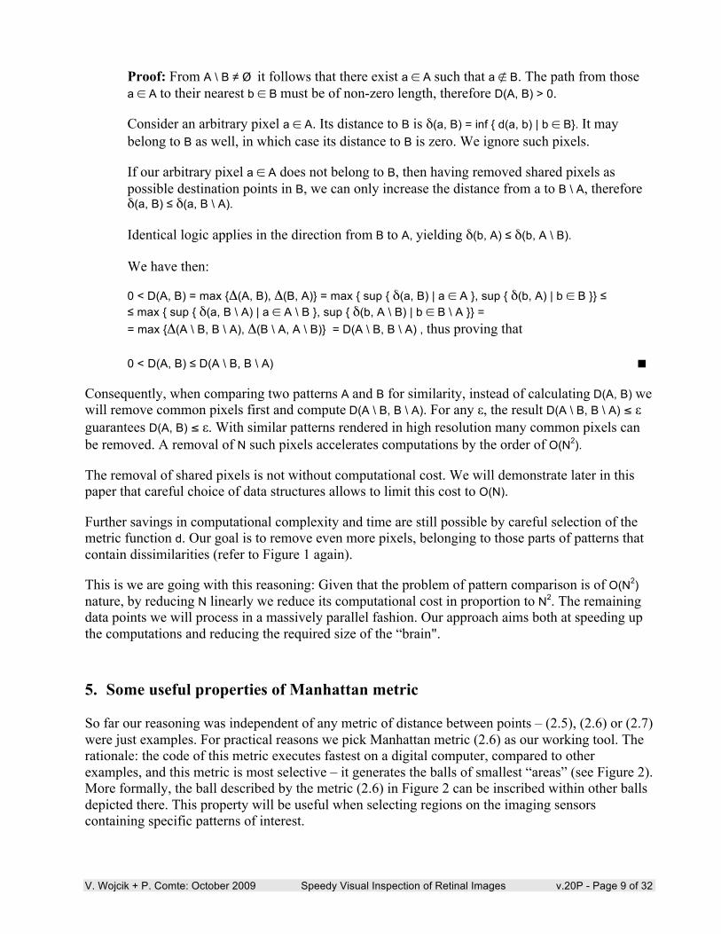
Proof: From A \ B ≠ Ø it follows that there exist a ∈ A such that a ∉ B. The path from those a ∈ A to their nearest b ∈ B must be of non-zero length, therefore D(A, B) > 0.

Consider an arbitrary pixel a ∈ A. Its distance to B is δ(a, B) = inf { d(a, b) | b ∈ B}. It may belong to B as well, in which case its distance to B is zero. We ignore such pixels.

If our arbitrary pixel a ∈ A does not belong to B, then having removed shared pixels as possible destination points in B, we can only increase the distance from a to B \ A, therefore δ(a, B) ≤ δ(a, B \ A).

Identical logic applies in the direction from B to A, yielding δ(b, A) ≤ δ(b, A \ B).

We have then:

0 < D(A, B) = max {Δ(A, B), Δ(B, A)} = max { sup { δ(a, B) | a ∈ A }, sup { δ(b, A) | b ∈ B }} ≤ ≤ max { sup { δ(a, B \ A) | a ∈ A \ B }, sup { δ(b, A \ B) | b ∈ B \ A }} = = max {Δ(A \ B, B \ A), Δ(B \ A, A \ B)} = D(A \ B, B \ A) , thus proving that

0 < D(A, B) ≤ D(A \ B, B \ A) ■

Consequently, when comparing two patterns A and B for similarity, instead of calculating D(A, B) we will remove common pixels first and compute D(A \ B, B \ A). For any ε, the result D(A \ B, B \ A) ≤ ε guarantees D(A, B) ≤ ε. With similar patterns rendered in high resolution many common pixels can be removed. A removal of N such pixels accelerates computations by the order of O(N2).

The removal of shared pixels is not without computational cost. We will demonstrate later in this paper that careful choice of data structures allows to limit this cost to O(N).

Further savings in computational complexity and time are still possible by careful selection of the metric function d. Our goal is to remove even more pixels, belonging to those parts of patterns that contain dissimilarities (refer to Figure 1 again).

This is we are going with this reasoning: Given that the problem of pattern comparison is of O(N2) nature, by reducing N linearly we reduce its computational cost in proportion to N2. The remaining data points we will process in a massively parallel fashion. Our approach aims both at speeding up the computations and reducing the required size of the “brain". 5. Some useful properties of Manhattan metric So far our reasoning was independent of any metric of distance between points – (2.5), (2.6) or (2.7) were just examples. For practical reasons we pick Manhattan metric (2.6) as our working tool. The rationale: the code of this metric executes fastest on a digital computer, compared to other examples, and this metric is most selective – it generates the balls of smallest “areas” (see Figure 2). More formally, the ball described by the metric (2.6) in Figure 2 can be inscribed within other balls depicted there. This property will be useful when selecting regions on the imaging sensors containing specific patterns of interest.


From now on, when speaking of the distance d(a, b) between points a = 〈x1, y1〉 and b = 〈x2, y2〉 we refer to and write explicitly (5.1) Manhattan distance: mh(a, b) = | x1 – x2 | + | y1 – y2 | as in (2.6). Similarly, we will use the notation (5.2) MH(A, B) = max {Δ(A, B), Δ(B, A)} when considering distances between sets A, B ⊂ S of points, as in (3.3). In this paper we will not use the formula (3.4). Observe that geometry textbooks do not define the concept of “straight” line – this concept is treated as axiomatically obvious to any reader. Euclidean geometry (based on metric (2.3)), for example, postulates that one can draw precisely one straight line between two distinct points a = 〈x1, y1〉 and b = 〈x2, y2〉, and the triangle law (2.4) reduces to the equality (5.3) d(a, b) =d(a, c) + d(c, b) only when the intermediate point c lies between a and b exactly on the straight line passing through a and b. If we want to travel from a to b passing through any c located elsewhere, we have no choice but to pay penalty in terms of the distance traveled, i.e. 5.4) d(a, b) <d(a, c) + d(c, b) In fact, in Euclidean space we can think of the “straight” line segment linking a and b as the shortest trajectory connecting a and b. This trajectory is unique. In Manhattan space things are different. When traveling from a to b we may only travel parallel to axes Ox and Oy, (see Figure 3), although we may change the direction of our motion at any moment. Figure 3 depicts several of many possible shortest (i.e. “straight”) paths, all of equal length. A Manhattan space may be continuous or discrete, the latter being of our interest. The points a and b define a rectangle, shown in yellow. It is provable that every point c contained in this rectangle can be treated as a convenient stopover point, i.e. there exists a trajectory from a to b via c for which the equality (5.3) holds. In fact, there are many such trajectories, all of them “straight”!

Fig.3. In discrete Manhattan space there are many “straight” paths from a to b, each of the same length.


The only time we will have no choice but to pay the distance penalty (5.4) on our travels from a to b is when choosing to stop at c outside of the yellow rectangle defined by a and b. We will make frequent use of this property of Manhattan metric. In our discrete Manhattan space the pixel distance function mh is integer-valued, and the smallest steps we can take are of unit length in the directions N, W, S, E (North, West, South, East). Every pixel in our space has exactly four immediate neighbours, i.e. pixels reachable from it in one step. We denote these neighbours of p by pix(p, N), pix(p, W), pix(p, S), pix(p, E). With these constructs in place, we can define an edge of an arbitrary but finite set A of Boolean-valued pixels in our discrete Manhattan space S. A pixel a ∈ A belongs to an edge of A if at least one of its immediate neighbours does not belong to A, or, symbolically: (5.5) edge(A) = { a ∈ A | val(a) and

(not (val(pix(a, N)) and val(pix(a, W)) and val(pix(a, S)) and val(pix(a, E)))) } The computation identifying edge(A) is not without cost. This cost can be minimized with careful selection of data structures used to represent A. Our consideration of this issue will later follow. We will find it useful to be able to inscribe arbitrary patterns within smallest possible rectangles. A rectangle in our Manhattan space can be defined by specifying its two diagonally opposite corners c1 and c2. Consider an arbitrary pattern A ⊂ S. The smallest rectangle that may contain A is a set in S defined as: (5.6) rect(A) = rect( { c1, c2} ), where the pixels c1 and c2 have the following coordinates:

c1 = < min (a.x | a ∈ A), min (a.y | a ∈ A) > c2 = < max (a.x | a ∈ A), max (a.y | a ∈ A) >

Equipped with these tools we strive to further reduce the computational effort needed to compute distance between arbitrary sets in discrete Manhattan space. Recall that on the basis of Theorem 2, having removed common pixels, we can limit our consideration to mutually exclusive sets in that space.

Theorem 3: For any two mutually exclusive patterns A, B ⊂ S we have Δ(A, B) = Δ(A, edge(B)).

Proof: Consider two points a ∈ A and b ∈ B maximizing the value of expression (3.2). That is, mh(a, b) = Δ(A, B). Could the point b lie in the interior of B? That is, could b ∈ B \ edge(B)? We will show that it is not possible. Suppose that it were so that b ∈ B \ edge(B). Then all four immediate neighbours of b would belong to B. One of those neighbours would be closer to a than b is. In that situation the two points a and b could not maximize the value of the expression (3.2), contradicting the first statement of our proof.


From that it follows that b cannot be the interior point of B, therefore b ∈ edge(B). But in this is the case Δ(A, B) = Δ(A, edge(B)) holds. ■

This is a very useful finding, as it allows us to remove even more pixels from the interior of mutually exclusive patterns when computing MH(A, B) as in (5.2). In short, for mutually exclusive patterns A and B we can compute (5.7) MH(A, B) = max { Δ(A, edge(B)), Δ(B, edge(A)) } instead of the formula (5.2), thus further reducing computing cost and time. However, if we attempt to compute (5.8) MH(A, B) = max { Δ(edge(A), edge(B)), Δ(edge(B), edge(A)) } this will not work. Consider, for example, a convex pattern A, entirely surrounded by pattern B. You will find that the pseudo-distance Δ(A, B) will stretch from the interior of A to the edge of B. The following will work:

Theorem 4: Given two non-empty patterns A and B such that rect(A) ∩ rect(B) = Ø, the following holds:

MH(A, B) = max { Δ(edge(A), edge(B)), Δ(edge(B), edge(A)) }

Proof: Observe that the condition rect(A) ∩ rect(B) = Ø implies mutual exclusivity of sets A and B but is stronger than that, i.e. this condition does not automatically hold for any pair of mutually exclusive sets A and B. Consider for example a rectangle in which two diagonally opposite corners constitute set A, and the remaining corners constitute set B. Both sets are mutually exclusive, but their rectangles are not. Consider therefore two points a ∈ A and b ∈ B maximizing the value of expression (3.2). That is, mh(a, b) = Δ(A, B). We already know that b ∈ edge(B). But now we ask: Could the point a lie in the interior of A? That is, could a ∈ A \ edge(A)? We will disprove this by contradiction, as in Theorem 3. Suppose that a ∈ A \ edge(A). It is possible then to execute one step of unit length from a in any direction and still remain within A. Given that a ∉ rect(B) and B ⊂ rect(B), at least one of these directions will lead away from rect(B), thus leading away from B. Having executed one step from a away from B we find ourselves further from B than a was. Therefore our two points a ∈ A and b ∈ B could not maximize the value of expression (3.2). That is, for these points mh(a, b) ≠ Δ(A, B), which contradicts our tentative assumption. It therefore follows that a must belong to the edge of A, i.e.: a ∈ edge(A). ■

The above theorems constitute powerful tools, permitting us to ignore many pixels of A and B, when computing their similarity, thus vastly shortening the computational cost and time.


6. Coding notation and fundamental pseudocodes Until now we were successfully reducing the computational complexity of the problem at hand by removing as many pixels as possible from patterns under consideration. Now we focus on reducing computational time, by exploit massive parallelism inherent in our formulae. The hardware and software of today is not entirely suitable for our purpose, so we resort to the following pseudocode: 6.1. Pseudocode notation We use standard notation, enhanced only in order to express parallelism and mutual exclusion to protect write access to shared variables. The notation

parbegin statement1; statement2; statement3; parend; statement4;

means that statements 1, 2 and 3 are to be executed in parallel, and the execution of statement 4 may begin only after all the three preceding statements in the parbegin block have terminated. Each of these three statements may be simple or a composite (i.e. a block). A composite statement is made of several statements (optionally preceded by declarations) and enclosed within begin and end. For example, let us write the pseudocode of the parallel function computing Euclidean distance between points in a 3D space. In this space each point P = 〈x, y, z〉 is an ordered triple, where x, y, z are the coordinates of P. In the pseudocode the notation P.x means the x –coordinate of point P.

function d1(P1, P2 : Point) return real is disx2, disy2, disz2 : real; begin parbegin disx2 := square(P1.x – P2.x); disy2 := square(P1.y – P2.y); disz2 := square(P1.z – P2.z); parend; return sqrt(disx2 + disy2 + disz2); end d1;

Several statements executing in parallel may attempt to modify some shared variables. To ensure integrity of such data we will enforce mutual exclusion of write access by using semaphores. A semaphore can store only non-negative values and can be initialized to any such value. Only two operations on a semaphore are possible: signal(s); -- increments the value of semaphore s by 1 wait(s); -- decrements the value of semaphore s by 1 as soon as -- it is possible to do so without yielding s negative More info on handling concurrency issues, such as access to shared variables, use of mutual exclusion and semaphores can be found in [8], [9].


Using a mutual exclusion semaphore we may provide conceptual pseudocode for the metric (2.7), now, as an example, between points in a 3D space:

function d3(P1, P2 : Point) return real is distance : real := 0; mutex : semaphore := 1; -- semaphore initialized to 1 begin parbegin begin disx : real := abs(P1.x – P2.x); wait(mutex); if distance < disx then distance := disx; end if; signal(mutex); end; begin disy : real := abs(P1.y – P2.y); wait(mutex); if distance < disy then distance := disy; end if; signal(mutex); end; begin disz : real:= abs(P1.z – P2.z); wait(mutex); if distance < disz then distance := disz; end if; signal(mutex); end; parend; return distance; end d3;

In this solution some sections of the code execute in parallel, but updating of the shared variable distance is protected by mutual exclusion. The three updates can be performed in arbitrary order. The scope of variables disx, disy, disz and of the semaphore mutex is the block within which they are declared, and its inner blocks. In our pseudocodes we will also use the parfor statement. The notation

parfor i in 1..10 do worker(i); parend; statement;

represents simultaneous launching of ten instances of the procedure worker, each with its own argument. It resembles the familiar for loop, but here the “iterations” are executed in parallel. As before, the execution of statement at end of this pseudocode may begin only after all ten worker processes in the parfor block have terminated. Finally, the familiar return statement is used to immediately terminate the execution of the procedure or function containing it, while returning the execution control to the calling environment. Additionally it terminates all parallel execution processes that were created as a result of calling the procedure or function. If used within a function, it also returns its computed value. As an example of use see pseudocode (9.8).


Observe that our pseudocodes are perfectly suitable for execution on a single-core CPU. The parfor block reduces then to the usual for loop, while the compound statements within a parbegin block can be executed in any order. 7. Pseudocodes for computing distances between sets For reasons to follow, we use integer-based metrics. The examples below reflect this already. The digital implementation of the set A being the argument of the function δ(x, A) defined in (3.1) is a finite set of n points (7.1) A = { a1, a2, … an } Using an arbitrary function d for computing distances between points, we can write the following pseudocode for computing δ(x, A) = inf { d(x, a) | a ∈ A } defined in (3.1): (7.2) function δ(x : Point; A : Set) return integer is distance : integer := ∞; -- initialized to infinity mutex : semaphore := 1; begin parfor i in 1 .. card(A) do -- card(A) is the number of elements in A dis : integer := d(x, a(i)); wait(mutex); if dis < distance then distance := dis; end if; signal(mutex); parend; return distance; end δ; We are now ready to define the pseudocode for Δ(A, B) = sup { δ(a, B) | a ∈ A } given in (3.2) as a pseudo-distance between two sets A = { a1, a2, … an } and B = { b1, b2, … bm }: (7.3) function Δ(A, B : Set) return integer is distance : integer := 0; mutex : semaphore := 1; begin parfor i in 1 .. card(A) do -- card(A) is the number of elements in A dis : integer := δ(a(i), B); wait(mutex); if dis > distance then distance := dis; end if; signal(mutex); parend; return distance; end Δ; Finally the distance D(A, B) between two sets defined in (3.3) can be implemented simply as: (7.4) function D(A, B : Set) return integer is


disAB, disBA : integer; begin parbegin disAB := Δ(A, B); disBA := Δ(B, A); parend; return max(disAB, disBA); end D; Following this logic, an arbitrary function d used to measure distance between points of a metric space has the properties (2.1), (2.2), (2.3) and (2.4) and induces another function D that can be used to measure distances between non-empty subsets of that space. That new function D also meets the requirements (2.1), (2.2), (2.3) and (2.4). Furthermore, if the function d can be implemented on a digital computer, then the function D can also be implemented, as per pseudocodes (7.2), (7.3) and (7.4). In our further analysis we therefore will only need to show how to implement the function d on a digital computer. That function induces the existence of the function D. 8. On comparison of patterns Pattern recognition and classification relies on routine use of pattern comparison algorithms. Prior to any comparison, two patterns must be optimally aligned. Any residual distance between two patterns is then a measure of their dissimilarity. Two patterns are deemed similar enough if their dissimilarity falls within tolerances of an application. The optimal alignment of patterns involves their linear to minimize the distance between them. This linear transformation may involve translation, rotation and scaling. The nature of the application dictates which of these three operations is admissible. Illustration: When comparing pair-wise the signatures in Figure 1 we might want to slide one signature onto another, in order to focus our attention on dissimilarities. Translation is therefore allowed here. The scaling is not allowed. We (humans) tend to sign documents in a similar way, regardless how much space for the signature is left on a document. Rotation is not allowed either: a signature oriented upside-down or at right angle would raise serious doubts about its validity. Similarly, humans are experts at face recognition, but not when faces are presented to us upside-down. In such situation we are unable to recognize even members of our immediate families. Consequently, prior to comparing any two patterns A and B we will assume that they are optimally aligned via pre-processing suitable to the application at hand. In any case, this pre-processing will include removal of common pixels (thus making A and B mutually exclusive) and, whenever allowed, the interior points of A and B.


8.1. Search strategies: Basic techniques for low-resolution patterns Conceptually the problem of comparing two optimally aligned patters has already been solved. Given two patterns A, B one needs to compute the distance D(A, B) between them as per pseudocodes (7.2), (7.3) and (7.4). If both sets A and B consist of a small number of N elements, further reduced by pre-processing, we could implement A, B as lists. The performance of the algorithm implementing the distance D(A, B) would be O(N2). Such delay is acceptable for small N, i.e. for low-resolution patterns. Things could be accelerated further. The function δ(x, A) = inf { d(x, a) | a ∈ A } defined in (3.1) could be implemented better: (8.1) function δ(x : Point; A : Set) return integer is distance : integer := ∞; -- initialized to infinity mutex : semaphore := 1; begin parfor i in 1 .. card(A) do -- card(A) is the number of elements in A dis : integer := d(x, a(i)); if dis = 1 then return 1; end if; if dis < distance then wait(mutex); if dis < distance then distance := dis; end if; signal(mutex); end if; parend; return distance; end δ; The function δ(x, A) scans all points in A looking for the one closest to x. Should it find the point in A distant by 1 from x, it immediately returns the value 1, which is the minimum value possible for mutually exclusive sets A and B. There is no need to peruse the remainder of points in A, which instantly become “uninteresting”. There is no gain in speed, if we can execute the parfor loop in perfect parallelism. Should we have fewer than card(A)processors, the speed gain can be noticeable. Indeed, the smaller the number of processors, the more noticeable it becomes. Optimal alignment of patterns A and B increases the probability of some points being immediate neighbours. The more of them, the faster our algorithm becomes. In principle, however, there is no guarantee that any points would be immediate neighbours: in that case the computation of the distance D(A, B) using (7.2) instead of (8.1) would be faster. When pressed for time, we should evaluate this distance twice and in parallel, using implementations (7.2) and (8.1). The computation of distance D(A, B) terminates whenever its result is returned first by one of the two parallel branches. Furthermore, there is no need for every parallel instance of the parfor block in the pseudocode (8.1) to update the shared variable distance, which holds the best distance value from x to A seen so far. The shared variable is protected by the semaphore mutex, which enforces mutual exclusion of access to update that variable. This mutual exclusion, when applied to all instances of the parfor block would amount to code serialization, resulting in a serious execution slow-down. In pseudocode (8.1) the mutually exclusive code is within an if statement, which inspects the value


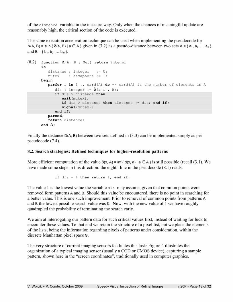
of the distance variable in the insecure way. Only when the chances of meaningful update are reasonably high, the critical section of the code is executed. The same execution acceleration technique can be used when implementing the pseudocode for Δ(A, B) = sup { δ(a, B) | a ∈ A } given in (3.2) as a pseudo-distance between two sets A = { a1, a2, … an } and B = { b1, b2, … bm }: (8.2) function Δ(A, B : Set) return integer is distance : integer := 0; mutex : semaphore := 1; begin parfor i in 1 .. card(A) do -- card(A) is the number of elements in A dis : integer := δ(a(i), B); if dis > distance then wait(mutex); if dis > distance then distance := dis; end if; signal(mutex); end if; parend; return distance; end Δ; Finally the distance D(A, B) between two sets defined in (3.3) can be implemented simply as per pseudocode (7.4). 8.2. Search strategies: Refined techniques for higher-resolution patterns More efficient computation of the value δ(x, A) = inf { d(x, a) | a ∈ A } is still possible (recall (3.1). We have made some steps in this direction: the eighth line in the pseudocode (8.1) reads: if dis = 1 then return 1; end if; The value 1 is the lowest value the variable dis may assume, given that common points were removed form patterns A and B. Should this value be encountered, there is no point in searching for a better value. This is one such improvement. Prior to removal of common points from patterns A and B the lowest possible search value was 0. Now, with the new value of 1 we have roughly quadrupled the probability of terminating the search early. We aim at interrogating our pattern data for such critical values first, instead of waiting for luck to encounter these values. To that end we retain the structure of a pixel list, but we place the elements of the lists, being the information regarding pixels of patterns under consideration, within the discrete Manhattan pixel space S. The very structure of current imaging sensors facilitates this task: Figure 4 illustrates the organization of a typical imaging sensor (usually a CCD or CMOS device), capturing a sample pattern, shown here in the “screen coordinates”, traditionally used in computer graphics.


Such sensors are actually xsmax by ysmax rectangular arrays of pixel sensors. In our example the pattern captured contains two pixels defining the sensor size. Normally, however, the captured pattern is contained inside the sensor area. Should our pattern of interest fail to fit the sensor region of the space S, we can take a finite number of partially overlapping images of it, and digitally stitch them together to form one composite image. Such digital stitching is routine today. Without any loss of computability we can therefore assume that any pattern of our interests is finite and fits some imaging sensor. In this paper we prefer to operate within the traditional systems of coordinates. Figure 5 depicts our environment for pattern recognition. The axes Ox and Oy are oriented in standard way. The central rectangle contains the smallest region of the imager containing a pattern in question – a pattern bounding box. This bounding box is surrounded by eight zones labeled N, NE, E, SE, S, SW, W and NW, which together tile the pixel space S. Our pattern (for simplicity not drawn in Figure 5) is positioned so that its pre-processed reference point is at the origin of the system of coordinates. As indicated before, the kind of pre-processing needed depends on the nature of the application. In the signature authentication illustration provided later in the paper, we align signature patterns so that their centers of mass coincide at origin. In signature pre-processing only linear shifts were allowed, but no scaling nor rotation. The scanned signatures were flipped around Ox axis to reflect the standard orientation of the Oy axis. This arrangement allows us to pre-process the pattern data with greater efficiency. Removal of common pixels from two patterns can be now done in O(N) steps, where N is the cardinality of the smaller of the two patterns: for each pixel in the smaller pattern we take its <x, y> coordinates and check whether the other pattern has a corresponding pixel. If so, we remove the shared pixel from both patterns.

Fig.4. Imaging sensor with a sample pattern, depicted in screen coordinates.

Fig.5. Standard pattern recognition environment.


Similarly, removal of the interior pixels from a given pattern is fast and easy: knowing the <x, y> coordinates of each pixel in a pattern we can immediately check whether all its immediate neighbours belong to that pattern: if so, that pixel can be removed. With complex and similar patterns the probability of point proximity increases. We take advantage of this. Having removed common pixels, we can now check for points in a given pattern distant by 1 from x. Should there be one, then the function δ(x, A) can immediately return the value 1, without wasting time to inspect the remainder of the pattern A. Failing that, the function checks for points distant by 2, 3 , … etc. from x. This is done by inspecting concentric circles of radii 1, 2, 3, etc. centered at point of interest x (peruse Figure 6). Observe that this algorithm always stops because our pattern being inspected is finite but non-empty and fits within its own bounding box (see Figure 5), defined by the points C1 = (xmin, ymin) and C2 = (xmax, ymax). The circles in Manhattan space (again see Figure 6) have “sides” (recall the ball d2 in Figure 2), which we will label NE, NW, SE, SW (North East, North West, etc.) The circumference of such a circle is 8*radius. Each side, of length 2*r, is made of r pixels only. Traversal of each side is easy: we merely need to keep modifying one coordinate (increasing or decreasing it by 1) while respectively modifying another coordinate, repeating that modification (preferably in parallel) r times. Even on a parallel pattern-matching machine with unlimited number of processors it does not make much sense to scan a circle of radius r+1 until a circle of radius r is inspected. However, all pixels belonging to a “side” of a circle can be inspected in parallel. Similarly, the four sides of a given circle can be inspected in parallel as well. Interestingly, in our discrete Manhattan pixel space S the areas of circles can, strangely enough, be measured in pixels too. We leave to the reader to find the formula to find the area of such a circle, as an exercise. To emphasize that we deal with pixel data, we will write δ(p, A) the, where is a pixel, and A is a set of pixels. The specification of the function δ(p, A) becomes: (8.2) function δ(p : Pixel; A : Set) return integer; As mentioned before, the point p may lay in the central rectangle of pattern A, or in any other zone adjacent to that rectangle (as per Figure 5). This is so, because p belongs to another pattern we are comparing to A. These patterns not being necessarily identical may lie within two rectangles that need not be congruent.

Fig.6. Circles of radii 1, 4 and 11 around a black pixel. All red pixels are distant 11 units from the black pixel.


Frequently the point p will fall within rect(A). In search for a point a∈A closest to p we draw concentric circles around p until one of them includes some a∈A as shown in Figure 7. The search terminates as soon as first such point a∈A is found. Note that as the radius of our search grows, some “sides” of our circles may lay (partially or entirely) outside of rect(A). We need to inspect only the parts of the sides within rect(A), knowing that there are no pixels of A outside rect(A). Given that rect(A) is convex there can be at most one segment of each side within rect(A). Knowledge of these facts permits us to write very efficient search code. Sometimes the point p falls into one of the zones N, S, E, W adjacent to rect(A). We project then p onto the rectangle yielding p’ and we inspect half-circles until we find a∈A closest to p’ (see Figure 8). Then we compute the distance: (8.3) d(p, a) = d(p, p’) + d(p’, a) because the points p, p’ and a are co-linear (in the Manhattan sense), i.e. the point p’ belongs to the rectangle defined by corners p and a (recall reasoning depicted in Figure 3). Whenever point p falls into one of the corner zones NE, NW, SE, SW (see Figure 9) we will denote as p’ the relevant corner of the rectangle and will limit ourselves to drawing only quarter-circles until we find a∈A closest to p’. Then again we will compute the distance d(p, a) using formula (8.3). 8.2.1. We can compute it even faster! The inspection of relevant half- or quarter-circles only can accelerate search considerably. We can do even better, though. Observe that for all pixels p in the corner zones NE, NW, SE, SW (see again Figure 9) the term d(p’, a) in the formula (8.3) will yield the same result for all p in each corner zone. Consequently, for each corner zone such search should be conducted only once and its outcome remembered.

Fig.8. Search situation with point p falling north of the rectangle of A: concentric half-circles may be used.

Fig.7. Search situation with point p falling within the rectangle of A: concentric circles must be used.


For the remaining N, S, E, W zones analogous (although a bit more complex) short-cuts are possible. As an illustration, consider the situation concerning zone S depicted in Figure 10. Suppose that previous search succeeded in finding a∈A closest to p0. Suppose further that now we seek a∈A closest to p. Observe that p’ belongs to the rectangle defined by points a and p0’, therefore the distance between p and a can be computed simply as (8.3). Why? Given that a is closest to p0’ and p’ is closer to a than p0’, then a must be closest to p’. In fact, for all p falling onto an infinitely tall blue rectangle shown on Figure 10 the formula (8.3) applies; no search is needed. Again, for all p falling within the rectangle defined by a and p0 (not shown on Figure 10) we can compute the distance d(p, a) directly, without any search. This finding is a useful tip: when inspecting sides of the circles our algorithms should report the positions of all pixels found, rather than merely reporting that the search was successful. These positions might be found useful later, obviating the needs for some subsequent searches. For all other p in zone S, such that p.x < a.x or p.x > p0.x there is no guarantee that a is closest to p, but the prior knowledge of existence of a allows us to estimate the upper limit of the computational effort needed to find a better a (if any). This is useful in processor scheduling. Of course that search should avoid inspecting regions already found to be empty (shown in dashed orange). The logic concerning zone S, presented as an illustration here, applies to zones N, E, W, with easy geometrical modifications. For p falling in the center zone we can find similar computational shortcuts. For example: for all p falling onto the blue rectangle defined by a and p0’ (see Figure 11), the pixel a is closest to p, the distance being d(p, a). No search is needed.

Fig.10. For all p falling within the blue region shown, the pixel a is closest to p, distant by d(p, a).

Fig.9. Search situation with point p falling northwest of the rectangle of A: concentric quarter-circles may be used.


Similar situations arise when p falls close to a corner of the center zone. Consider the previous search situation depicted in Figure 9, which resulted in finding some point a∈A (not shown). We envisage a rectangle defined by that a and p’. Should any new p fall onto that rectangle, then a is closest to that p, no search needed. Finally, consider the situation in which previous search called for using full circles (Figure 12). The previous logic still applies. Specifically: Suppose the former search for a∈A closest to p0 resulted in finding a as shown. Then, for any new p falling onto the blue rectangle defined by p0 and a there is no need to perform any search: we already know that the same a is still relevant. Remember further that any search, like the one shown in Figure 12, may result in several a found, all equidistant from its origin. In that situation several blue rectangles can be drawn. Should a new search be required then the first thing to do is to check whether the new origin falls onto any one of the blue rectangles. Clearly, the information about “voids” within a scanned pattern is valuable, as it can be used to avoid performing repetitive but redundant searches. An open question arises, for future investigation: Under what conditions an additional pre-processing of patterns aimed at discovery of these voids would be beneficial? By the nature of things, patterns do not fill their rectangles completely – this means that some voids are initially there. Such voids are further expanded (and new voids created) by removing shared pixels from patterns, and by removing (whenever possible) the interior pixels from patterns. When would a pre-processing exercise of void identification by inscribing a number of largest possible empty circles within a pattern increase overall computational speed? How many of such empty circles should we attempt to inscribe? What is the minimum radius of a circle worth inscribing? The answers to these questions depend on the

Fig.12. For all p falling within the blue rectangle defined by p0 and a, the pixel a is closest to p, distant by d(p, a).

Fig.11. For all p falling within the blue rectangle defined by p0’ and a, the pixel a is closest to p, distant by d(p, a).


nature of patters (i.e. the environment the system inhabits), the resolution of their imaging sensors and on the computing performance characteristics of the system (i.e. the degree of adaptation of the system to its environment). This concludes our outline of strategies applicable to accelerating search computations when using Manhattan metric. Ours is a gross simplification of the biological vision: animal retinas contain sensors arranged in a hexagonal grid. In that situation the pixel space can be subdivided into 19 zones, and massively parallel computers are needed to handle such problems. 9. Application example: Signature authentication We illustrate the power of our basic strategies with a practical problem of pattern recognition, clustering and classification of universal interest. We chose a problem of signature authentication. Signatures are relatively simple patterns, and in their study we can skirt a number of pre-processing issues of computer vision: extraction of patterns from their backgrounds, pattern translation, rotation and scaling, handling of image noise, of colour, of contrast and exposure, etc. We know how to handle these important issues, but this is a topic for another paper. Despite of its simplicity, the problem of signature authentication is of immediate practical applicability and interest. Or is this simplicity deceptive? Signatures are routinely used in banking. Banking is a discipline older than computer science, so surely bankers must have developed over time some standard methods for signature authentication… We aimed to compare the reliability of our methodology to a reliability of a trained expert banker (a human), treated as a control. Unfortunately, we could not find any study evaluating effectiveness of bank clerks in signature authentication, or identification of so skilled clerks. In fact, it seems that the bankers do not attempt to verify signatures on all documents passing through their hands, but merely look at signatures only on documents that are found problematic otherwise. A clerk in a bank where you have an account is responsible of serving several hundred (perhaps more?) customers like you. Each of these people cannot sign exactly in the same way twice while the signature forgeries are likely to resemble genuine signatures. What is the chance that the clerk intricately knows your signature, as well those of all his other customers, to reliably judge each signature as genuine or a fake? Facing this reality we cannot offer a traditional, comparative study of our signature authentication methodology vs. that of a trained human, treated as a control. We can, however, present the reliability of our system in absolute terms. To that end we gathered the signatures of 21 persons, whom we know well. This is too small a sample to offer statistically firm findings but only 21 persons permitted us to use their signatures in our study. We then decided to focus on the trends only. Each participant in our study deposited a signature eight times (four times when “opening an account” with us, and four more times simulating subsequent “transactions”). We (the authors) also forged some of their signatures, and also asked some randomly chosen participants to forge some signatures of other participants. In this way for each participant we had 12 signatures: 8 genuine and


4 forgeries. We could tell for sure which is which, because we witnessed their creation. Thus, to test our system we had a pool of 252 signatures in total. A priori, our system can recognize a valid signature as such, or a forgery as a fake. In both cases it is deemed successful. It can also commit type I error (judging a valid signature as fake) or type II error (diagnosing a forged signature as genuine). In the latter two cases the system would be unsuccessful. The overall reliability of the system is the probability of it being successful when presented a sequence of signatures. This allows us to measure the reliability in absolute terms; moreover, it allows conducting simulation studies of account handling procedures that would enhance banking security. Note that the bankers are acutely concerned with type II errors only: these errors make them lose money. The errors of type I merely annoy the customer, who on second thought may actually congratulate a banker on his vigilance. Using this theory we offer the methodology for automated signature authentication. In current banking practice, both signature and customer name appear on a document, and the signature is merely used for a visual verification by a bank clerk that a given customer authored the document. That document may bear correct mailing address of the sender and other information facilitating the signature validation task, which is simpler than the problem of customer identification given signature only (or a fingerprint, a photograph, etc.), but still error-prone. Or system is very ambitious: it identifies the customer on the basis of the signature alone. It compares signatures to reference signatures. Each signature S is scanned in black and white at 300 dpi resolution and is stored as a set S = {p1, p2, … pn} of black pixels pi = 〈xi, yi〉 where xi, yi are integer-valued pixel coordinates. Different signatures consist of varying number and positions of black pixels. All signatures in the system were preprocessed to make their centers of mass coincide. Their relative positioning information was thus deliberately lost. Neither signature rotation nor scaling was allowed. We used the integer-valued Manhattan metric (2.6) to measure distance between pixels. This induced a particular metric D (as per 3.3) to be used for measuring distance between signatures. With the positioning information lost, D can be seen as a measure of dissimilarity between signatures. In this vein two signatures S1 and S2 are deemed to belong to the same person if they are sufficiently similar, i.e. D(S1, S2) ≤ ε where ε is a properly chosen small value. 9.1. Opening an account in the traditional way A new customer is requested to provide four reference signatures S1, S2, S3, S4 that are certified on the spot by a witnessing clerk. We made the system open an account in three ways: using two, or three, or four signatures of a given customer. Using these balls the system create a new customer signature profile C consisting of balls that partially overlap. The customer profile consisting of three balls follows: (9.1) C = { B1(S1, r1), B2(S2, r2), B3(S3, r3) } where

r1 = min ( D(S1, S2), D(S1, S3) ) r2 = min ( D(S2, S1), D(S2, S3) ) r3 = min ( D(S3, S1), D(S3, S2) )

The pseudocode for creating this signature profile is as follows:


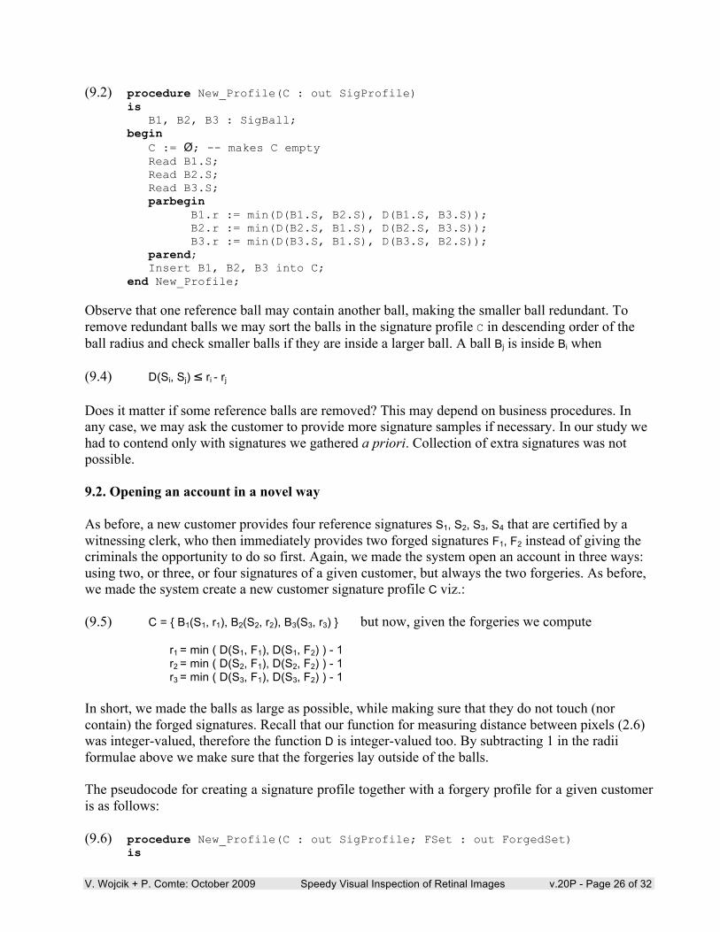
(9.2) procedure New_Profile(C : out SigProfile)

is B1, B2, B3 : SigBall; begin C := Ø; -- makes C empty Read B1.S; Read B2.S; Read B3.S; parbegin B1.r := min(D(B1.S, B2.S), D(B1.S, B3.S)); B2.r := min(D(B2.S, B1.S), D(B2.S, B3.S)); B3.r := min(D(B3.S, B1.S), D(B3.S, B2.S)); parend; Insert B1, B2, B3 into C; end New_Profile;

Observe that one reference ball may contain another ball, making the smaller ball redundant. To remove redundant balls we may sort the balls in the signature profile C in descending order of the ball radius and check smaller balls if they are inside a larger ball. A ball Bj is inside Bi when (9.4) D(Si, Sj) ≤ ri - rj

Does it matter if some reference balls are removed? This may depend on business procedures. In any case, we may ask the customer to provide more signature samples if necessary. In our study we had to contend only with signatures we gathered a priori. Collection of extra signatures was not possible. 9.2. Opening an account in a novel way As before, a new customer provides four reference signatures S1, S2, S3, S4 that are certified by a witnessing clerk, who then immediately provides two forged signatures F1, F2 instead of giving the criminals the opportunity to do so first. Again, we made the system open an account in three ways: using two, or three, or four signatures of a given customer, but always the two forgeries. As before, we made the system create a new customer signature profile C viz.: (9.5) C = { B1(S1, r1), B2(S2, r2), B3(S3, r3) } but now, given the forgeries we compute

r1 = min ( D(S1, F1), D(S1, F2) ) - 1 r2 = min ( D(S2, F1), D(S2, F2) ) - 1 r3 = min ( D(S3, F1), D(S3, F2) ) - 1

In short, we made the balls as large as possible, while making sure that they do not touch (nor contain) the forged signatures. Recall that our function for measuring distance between pixels (2.6) was integer-valued, therefore the function D is integer-valued too. By subtracting 1 in the radii formulae above we make sure that the forgeries lay outside of the balls. The pseudocode for creating a signature profile together with a forgery profile for a given customer is as follows: (9.6) procedure New_Profile(C : out SigProfile; FSet : out ForgedSet)

is


B1, B2, B3 : SigBall; F1, F2 : Signature; begin C := Ø; -- makes C empty FSet := Ø; -- makes FSet empty Read B1.S; Read B2.S; Read B3.S; Read F1; Read F2; parbegin B1.r := min(D(B1.S, F1), D(B1.S, F2)) - 1; B2.r := min(D(B2.S, F1), D(B2.S, F2)) - 1; B3.r := min(D(B3.S, F1), D(B3.S, F2)) - 1; parend; parbegin Insert B1, B2, B3 into C; Insert F1, F2 into FSet; parend; end New_Profile;

The bankers might want to replace redundant balls in the signature profile with more relevant balls. In our study this was not possible, all the signatures having been collected upfront. Additionally, should some radii of the reference balls be too small, the banker may advise the customer that her/his signatures can easily be falsified. 9.3. Authenticating signatures To be deemed valid each new signature of our customer must fall within at least one of the reference balls. A new signature X falls within a ball Bi(Si, ri) when (9.7) D(Si, X) ≤ ri

therefore the authentication pseudocode is simply: (9.8) function Valid(X : Signature; C : SigProfile) return Boolean

is begin parfor i in 1 .. card(C) do if D(X, C.B(i).S) ≤ C.B(i).r then return True; end if; parend; return False; end Valid;

9.4. Learning from errors No intelligent system, biological or otherwise, is perfect. They all make mistakes - ours is no exception. However, an intelligent system will make a given mistake only once. This is how: Eventually the validity of a given signature X will be contested, by a complaint arriving from the environment of our system (the customer). Two situations are possible here:

1. Our system authenticated a forged signature, or 2. A valid signature has been rejected.


In the first situation we have to insert the forged signature X into the set of forgeries, and reduce the size of some reference ball(s) accordingly, perhaps deleting some balls that became redundant. If the customer account was opened in the traditional way, then initially the set of forgeries is empty, thus making the system more vulnerable. Nevertheless, it can and will learn, although possibly at higher cost to the banker. In the second situation, we update the customer signature profile by inserting a new ball into it. In case of authentication challenge, we will use the function Valid to determine which of the two situations we are facing. The pseudocode is: (9.9) procedure Fix(X : in Signature; C : in out SigProfile; FSet : in out ForgedSet)

is B : SigBall; mutex : semaphore := 1; begin if Valid(X, C) then –- we are in situation 1 parfor i in 1 .. card(C) do C.B(i).r := min(C.B(i).r, D(X, C.B(i).S) – 1); parend; Insert X into Fset; else -- we are in situation 2 B.S := X; B.r := ∞; -- set initially to infinity parfor i in 1 .. card(FSet) do radius : integer := D(X, Fset.F(i)) – 1; wait(mutex); if B.r > radius then B.r := radius; end if; signal(mutex); parend; Insert B into C; end if; Sort C in descending order of ball radius; Remove redundant balls (if any) from C; end Fix;

With this functionality we get a banking system that continuously learns about customer signatures, is better and better at their authentication, and may even advise some customers that their signatures might easily be forged. It can also forget signatures of customers that closed their accounts, to keep its adaptation to the work environment. Indeed, it could also add the signatures of its ex-customers to the bank of forgeries, to keep improving its reliability. 9. 5. Results Let us pause for a moment and try to predict what kind of results we should expect. Pure genetic programming systems, neural networks, ant colonies, particle swarms, etc., give good results when exposed to relatively small training and test sets of data, but are laborious to train, and tend to fall apart under ever increasing training and testing workloads [10]. Our banking system is more human-like. Its instance-based training is fast and straightforward (it merely learns about new objects by inserting relevant balls into its knowledge bank), but like


humans, suffers from the “little knowledge is a dangerous thing” syndrome. Unlike most machine learning algorithms in use today, it is capable of continuous learning, and to keep improving its performance. Suppose some bank adopts our system. When presented the signatures of its first customer, the system knows that it should use these signatures as centers of balls to be inserted into its knowledge bank, but what should be the radii of these balls? Infinity seems plausible, as the system knows of only one customer. But, if infinity were plausible, then one ball to represent that customer would suffice… However, with an infinitely large ball the system would be unable to spot forgeries, even of its single customer. Like any poorly trained human, our system is susceptible to “jumping to conclusions”. Some caution must then be used here. We ask the customer to offer several sample signatures, as per pseudo-code (9.2) and create several balls of finite size around these signatures. We know, however, that these signatures are unlikely to be the most representative signatures penned by that customer, i.e. we have been overly conservative in determining the ball radii, which should be multiplied by a certain “caution coefficient” α. To estimate the optimal value of that coefficient, we divided the data set of signatures into a training set of 5 randomly selected signatures, found the value of α maximizing the overall diagnostic reliability of our system over that training set, and then exposed our system to the customers from the test data in random order. For handling accounts one account at a time, the results are shown in Table 1. The case of no forgeries used at opening of the account amounts to the use of conventional banking method.

Table 1: Overall reliability of signature authentication when handling one customer account at a time. Note that the bank is vulnerable to a financial loss only then committing type 2 error; type 1 error merely annoys the customer.

Observe that these results are somewhat vulnerable to the choice of customers in our training set, and to the order in which test customers are then presented to the system. Also, a self-respecting banking system should keep refining its knowledge and fine-tune its caution coefficient α while doing business (i.e. performing test transactions). This is what continuous learning is all about. We tried to increase the system reliability by reducing the dangers stemming from having “too little knowledge” by opening the accounts of all customers first, and only then allowed the bank to do business, by exposing it in random order to transaction of customers from the test set. This simulates the conversion to our system by an existing bank. The ball radii for all customers are typically smaller, because balls belonging to a given customer must be mutually exclusive with balls belonging to other customers, thus making our system overly cautious. The effect of not having the most representative signatures of our customers becomes clearly visible.


The Table 2 shows the results:

Table 2: Overall reliability of signature authentication when opening all customer accounts at once. This seems to be the natural way of handling related vision problems, since the environment was already complex (i.e. consisted of many objects) when vision evolved.

Unfortunately, this attempt was not successful. The overall reliability of the system suffered, although the system did not commit any costly type II errors. This is not the forum to convince any banker to convert to our system on the training basis of five customers only. Given that humans do not consistently pen their signatures, the system will need more valid samples, acquired while doing business. This inconsistency makes it impossible to reliably verify signatures (humanly or by a machine) on the basis of two, three or four valid samples. That is why we tend to focus on fingerprints, iris scans, and other biometric data when trying to identify humans. In any case, every banker will be glad to hear that our system is very unlikely to commit costly type II errors. Conversion to our system is possible, but the set of valid signatures of each customer must contain many more samples, taken from their uncontested transactions. 10. Conclusion We have proposed here a novel methodology for creating intelligent systems. This methodology:

1. Emerges through the simulation of some aspects of functionality of human visual cortex; 2. Is very basic: it uses only set theory and the concept of metric spaces, and as such, lies at the

foundation of all mathematics, thus ensuring its wide applicability; 3. Is relevant to problems of pattern recognition, identification, clustering and classification

outside of the vision domain; 4. Suggests that intelligent systems need not be wet nor carbon based; 5. Offers a way of breaking out from the current impasse in computer linguistics [8]; 6. Leads to systems and algorithms that are:

o massively parallel; o capable of continuous (on the job) learning; o capable of selective forgetting of less useful facts, and so of maintaining their adaptation

to environments that evolve sufficiently slowly; o fault tolerant; o scalable (upward and downward) to the parallel computer at hand;


We have focused mainly on machine learning. Forgetting less useful facts is equally important for real-time systems keen to maintain their adaptation to an evolving environment. Banking application was just an example of this. In general, we propose to keep track of usefulness of various balls in the knowledge banks of our systems so as to keep the working set of balls in the systems’ ”short term memories”. The concept of a working set is well known. Details at [9], [10]. As it turns out, it is easier to create reliable but rigid and less intelligent systems with hard-coded knowledge, than adaptive intelligent systems that would learn from their own experience. Such systems will likely need extensive training before being put in the position of responsibility. REFERENCES [1] http://www.nikonusa.com/ as of 30 Aug 2008. [2] http://www.microtekusa.com/ as of 30 Aug 2008. [3] http://www.usa.canon.com/ as of 30 Aug 2008. [4] http://www.red.com/ as of 30 Aug 2008. [5] http://www.veterinaryvision.com/See.htm as of 30 Aug 2008. [6] http://en.wikipedia.org/wiki/Mantis_shrimp as of 30 Aug 2008. [7] A.M. Gleason, Elements of Abstract Analysis, Jones and Bartlett Publishers, Boston 1991. [8] http://www.sysmannews.com/content/article.aspx?ArticleID=32043 as of 30 Aug 2008. [9] A.M. Lister, R.D. Eager: Fundamentals of operating systems, 4th ed., Macmillan 1988. [10] W. Stallings: Operating systems: Internals and design principles, 5th ed,

Pearson / Prentice Hall, 2005. [11] Xin Yao, Yong Liu: A New Evolutionary System for Evolving Artificial Neural Networks,

IEEE Transactions on Neural Networks, Vol.8, No. 3, may 1997. [12] R.O. Duda, P.E. Hart, D.G. Stork: Pattern Classification, 2nd ed., John Wiley & Sons 2001. [13] K. Fukunaga: Statistical pattern recognition, 2nd ed., Academic Press, 1990. [14] J.C. Russ: The image processing handbook, CRC Press, 1992. [15] B.V. Dasarathy: Nearest neighbor (NN) norms: NN pattern classification techniques,

IEEE Computer Society Press, 1991. [16] R. Klette, P. Zamperoni: Handbook of image processing operators, John Wiley & Sons,

1996.


[17] H.R. Schiffman: Sensation and Perception - An Integrated Approach, 5th ed.,

John Wiley & Sons, Inc. ISBN: 0-471-24930-0 [18] I. Aleksander (ed.): Neural computing architectures: The design of brain-like machines,

MIT Press, 1989. [19] E.R. Davies: Machine vision: Theory, Algorithms, Practicalities, Academic Press, 1990. [20] H. Freeman (ed.): Machine vision for three-dimensional scenes, Academic Press, 1990. [21] V.K.P. Kumar (ed.): Parallel architectures and algorithms for image understanding,

Academic Press, 1991. [22] V. Kumar, P.S. Gopalakrishnan, L.N. Kanal: Parallel algorithms for machine intelligence

and vision, Springer Verlag, 1990.

visual pattern recognition and learning - computer science

Documents