Visual Odometry In SelfDriving Car

Indian Institute of Technology, Kanpur

Undergraduate Course Project

Anurendra Kumar(12147)

Mentor - Prof. Gaurav Pandey

Abstract

This is the documentation of the work we have done to implement visual odometryin the self driving car project. Currently we have tested monocular visual odometryon the Ford Campus Vision and Lidar dataset. The implementation is in C++ usingOpencv library and works in real time. We used only the camera information to predictthe motion of car without any prior knowledge of surrounding and other sensor data.We have used FAST and SIFT to detect features. KLT tracker with RANSAC foroutlier rejection is employed for tracking features.

Contents1 Introduction 2

2 Motivation 2

3 Problem Formulation 2

4 Fundamentals 34.1 Camera Calibration . . . . . . . . . . . . . . . . . . . . . . . . . . . . . . 3

5 Methodology 45.1 Feature Detection . . . . . . . . . . . . . . . . . . . . . . . . . . . . . . . 5

5.1.1 SIFT Feature Detector and descriptor . . . . . . . . . . . . . . . . 55.1.2 Fast Feature Detector . . . . . . . . . . . . . . . . . . . . . . . . . 7

5.2 Feature Tracking . . . . . . . . . . . . . . . . . . . . . . . . . . . . . . . 85.2.1 Kanade Lucas Tomashi(KLT) Tracker . . . . . . . . . . . . . . . . 8

5.3 Motion Estimation . . . . . . . . . . . . . . . . . . . . . . . . . . . . . . 95.3.1 Epipolar Geometry . . . . . . . . . . . . . . . . . . . . . . . . . . 95.3.2 Essential matrix computation . . . . . . . . . . . . . . . . . . . . . 105.3.3 Trajectory Estimation . . . . . . . . . . . . . . . . . . . . . . . . . 11

6 Experiments and Results 126.1 Dataset . . . . . . . . . . . . . . . . . . . . . . . . . . . . . . . . . . . . 126.2 Experimental Setup . . . . . . . . . . . . . . . . . . . . . . . . . . . . . . 136.3 Results . . . . . . . . . . . . . . . . . . . . . . . . . . . . . . . . . . . . . 13

7 Discussion 15

8 Conclusions and Future work 16

9 Acknowledgement 16

1

1 IntroductionVisual Odometry is the process of estimating the vehicle’s trajectory using a single or mul-tiple camera rigidly attached to the vehicle. Similar to wheel odometry, visual odometryincrementally estimates the position of the vehicle without taking into account of the pastinputs. In Monocular Visual Odometry, the path obtained is a scaled version of the groundtruth. Visual Odometry was first used by NASA in Rovers Mars.

2 MotivationIn self driving car, the challenge is to solve the problem of braking, steering and accel-erating which are done automatically without driver attention. All of the three paradigmsrequire correct absolute path prediction. Other techniques which can be employed for sametask are :

• Wheel odometry - It has slipping problem in uneven terrain

• Global Positioning System(GPS) - It is erroneous and not always available

• Inertial Measurement Unit(IMU) - I.M.U’s which generate accurate path are gener-ally too costly. There are some I.M.U’s which are available at comparatively moder-ate cost but the path generated by them is often erroneous.

Figure 1: Normal I.M.U. and high cost I.M.U.

Visual odometry promises appropriate results in almost all kind of environments with rela-tively low cost apparatus(cheap sensors in comparison to other sensors). This has resultedin increasing focus of research in the area. V.O works correctly when we have sufficientillumination and enough number of interesting points (features) in the frames. Also theconsecutive frames should have overlap of common features, which enables us to trackthose features. The aim of this undergraduate project is to solve the problem of predictingtrajectory in self driving car using visual inputs alone in for monocular system.

3 Problem FormulationThe camera is mounted on the moving car and takes images with certain fixed framesper second to have sufficient overlap of scenes in two consecutive frames. Let the setof images be I0, I1, ........In. The aim is to estimate the transformation matrices relating

2

the consecutive camera poses which will be utilised to estimate the trajectory of the car.Without loss of generality we can assume that camera co-ordinates is same as vehicle’s co-ordinate frame except for some translation. Let’s denote the camera pose as C0,C1, ......Cn.The two consecutive camera poses are related as

Cn =Cn−1Tn

where

Tk =

(Rk,k−1 tk,k−1

0 1

)is the transformation matrix consisting of rotation matrix Rk,k−1 and translation vector tk,k−1between instants k and k-1. C0 is the initial camera pose . If we are able to find T1, ..Tnthen any camera pose Cn can be computed by concatenating C0,T1,T2, ...Tn and thus we canfind the trajectory by finding all the camera poses. We find some keypoints(discussed later)pi

k and pik−1 and utilize those to find transformation matrix Tk. Tk is found by minimizing

the L2 norm between the 2D feature sets pik and pi

k−1 and solve the following objectivefunction [8]

Tk = argminTk

∑i||pi

k−Tk pk−1i|| (1)

4 FundamentalsIn order to arrive at the correct transformation matrices we use the perspective cameramodel to map 3d points in universe to 2d points in camera pixels.

Figure 2: Image Projection Model

src : https://www.ics.uci.edu/ majumder/vispercep/cameracalib.pdf

4.1 Camera CalibrationFigure 2 shows the pinhole model of a camera. O is called the center of projection ofcamera and the image plane is always at a distance of f (focal length) from O. A point in

3

3D P(X,Y,Z) (in camera’s frame) is viewed in image plane as Pc(u,v) (here we assume thatimage plane origin (O

′) is the point(α) where principal axis intersects image plane). By the

property of similar triangles,

fZ=

uX

=vY

u =f XZ

, v =fYZ

The above equations can be represented in homogeneous coordinates as

Ph =

u′

v′

w

=

f 0 00 f 00 0 1

XYZ

= KP

Pc =

(uv

)=

(u′

wv′

w

)If the origin(O

′) of image plane does not coincide with α then we need to adjust Pc

accordingly by

u =f XZ

+ cx, v =fYZ

+ cy

where (cx,cy) is the position of α (called principal point) from O′. notice that Pc we derived

until now is not exactly the point in the image because u v are in inches (or MKS system).So we need to correct that factor by multiplying mx my which are pixels/inch in x and ydirections respectively. So the overall rectified equations now looks like

u = mxf XZ

+mxcx, v = myfYZ

+mycy

In matrix form it is represented as

Ph =

u′

v′

w

=

mx f 0 mxcx0 my f mycy0 0 1

XYZ

= KP

This K matrix is called intrinsic camera calibration matrix. If the camera’s coordinateframe is not aligned with vehicles coordinate frame then we have to perform rotation andtranslation to align the above two frames. These matrices are called extrinsic calibrationmatrix. In this project, we are not making use of the extrinsic calibration matrix as thereis only translation vector required to align camera frame with vehicle frame which donoteffect our generated path.

5 MethodologyWe were provided images which are adjusted for distortion. A brief outline of the algorithmfollowed is :

• Feature detection- Detect a considerable amount of features in the images. If num-ber of features fall below a certain threshold a redetection is triggered.

• Feature tracking- Track the detected features in consecutive images It and It−1.

4

• Epipolar Geometry- With the pairs of tracked points obtained from above step, useNister’s five point algorithm with RANSAC to find essential matrix.

• Estimating Motion Trajectory- Extract rotation matrix and translation vector fromthe essential matrix and concatenate it to find the trajectory of motion.

5.1 Feature DetectionInstead of tracking all of the pixels we rather focus on features which are interesting parts ofimage that differ from immediate neighbourhood. To employ the repeatability of featureswe need invariance(Translational, Rotational, Scale and intensity invariance ) and robust-ness of the features. Feature detectors can be broadly divided into two types as follows:-

• Corner detectors such as Harris (based on eigen values of second moment matrix)and FAST detector, because corners are relatively invariant to change of view. Theyare translational and rotational invariant but not scale invariant.

• Scale Invariant Detectors such as SIFT.

5.1.1 SIFT Feature Detector and descriptor

• SIFT Detector: Outline of SIFT detector:

– Construct a scale space:- To achieve scale invariance, SIFT finds best scaleto detect feature. To create a scale space, the resized images are progressively”blurred” out. Mathematically, ”blurring” is done by the convolution of Gaus-sian Kernel with image

L(x,y,σ) = G(x,y,σ)∗ I(x,y) (2)

where L is blurred image,I is image,x and y are pixels,σ is scale and G(x,y,σ)is the gaussian kernel as:-

G(x,y,σ) =1

2πσ2 e−(x2+y2)/2σ2

(3)

– LoG and DoG operations:- The Laplacian of Gaussain(LoG) operation calcu-lates second derivatives of gaussian which detects corners and edges, the poten-tial points for features. LoG is given by :

LoG(x,y) = ∇2L(x,y) = Lxx +Lyy (4)

But as we see, L is dependent on scale factor σ . So, to account for this, wemultiply LoG(x,y) by σ2 to produce scale-normalised LoG given by :

LoG(x,y,σ) = σ2∇

2L(x,y) = σ2(Lxx +Lyy) (5)

But since second derivative is computationally expensive, LoG can be approx-imated with Difference of Gaaussian(DoG). DoG is obtained by difference ofblurrings at different scales depicted in the figure below:-

DoG(x,y,σ) = (G(x,y,kσ)−G(x,y,σ))∗ I(x,y) = L(x,y,kσ)−L(x,y,σ) (6)

5

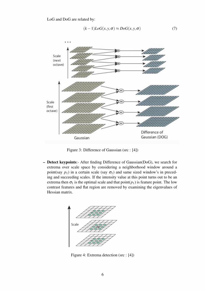
LoG and DoG are related by:

(k−1)LoG(x,y,σ)≈ DoG(x,y,σ) (7)

Figure 3: Difference of Gaussian (src : [4])

– Detect keypoints:- After finding Difference of Gaussian(DoG), we search forextrema over scale space by considering a neighborhood window around apoint(say p1) in a certain scale (say σ1) and same sized window’s in preced-ing and succeeding scales. If the intensity value at this point turns out to be anextrema then σ1 is the optimal scale and that point(p1) is feature point. The lowcontrast features and flat region are removed by examining the eigenvalues ofHessian matrix.

Figure 4: Extrema detection (src : [4])

6

• SIFT DescriptorFor describing a SIFT feature mathematically, a 16 x 16 window around the detectoris taken and divided into 4 x 4 grid cells. In each cell, the gradient orientations for allpixels calculated and are quantized to 8 bins. A frequency histogram of orientationsis calculated for each of the cell. Concatenating the values of histogram frequenciesin all cells gives 16 x 8 =128 dimensional vector for a SIFT descriptor. :[4] ).

Figure 5: SIFT descriptor

src : http://www.codeproject.com/KB/recipes/619039/SIFT.JPG

5.1.2 Fast Feature Detector

SIFT and Harris corner are computationally expensive and time taking. FAST[7] detectoris often used for real time video processing because of high speed performance. To find acorner it uses the heuristic that a corner will have a continuous set of brighter set of pixels ordarker set of pixels than its own. It constructs a circle of 16 pixels and checks if it satisfieseither of the following conditions:

• A set of N contiguous pixels which has brightness greater than the corner with atleast a certain threshold.

• A set of N contiguous pixels which has brightness lesser than the corner with atleast a certain threshold. The number of contiguous pixels,N and threshold are hyperparameter.

Figure 6: Fast feature detector (src : [7]

7

A High speed test for FAST [2] : To exclude a large number of non-corner points, itchecks only for the points 1,9,5 and 13. It first checks if 1 and 9 are too brighter or darkerthan center pixel, if so, then it checks for 5 and 13. If the center pixel is corner then eitherof these pixels must be brighter or darker than certain threshold. Though it exhibits highperformance but it has several weaknesses, prominent among them are:-

• It doesn’t reject many candidates for N < 12

• The pixels selected are not optimal since corners might be tilted

Machine learning approaches are used to solve these problems.

5.2 Feature TrackingAfter detecting the potential keypoints our aim is to estimate the point translation in con-secutive frames. We have employed KLT tracker [9] to track the features.

5.2.1 Kanade Lucas Tomashi(KLT) Tracker

KLT tracker assumes following conditions:-

• Brightness Constancy- The same point projected in different frames looks same.

• Small Motion- The movement of point is not very far.

• Spatial Coherence- The motion of points are similar to their neighbour.

From brightness constancy we get

I(x,y, t) = I(x+u,y+u, t +1) (8)

where x,y are pixel points,t is the time instant and u,v are displacement of the points.Assuming small motion and expanding R.H.S. using taylor series gives

I(x+u,y+ v, t +1)≈ I(x,y, t)+ Ix.u+ Iy.v+ It (9)

Solving the above equation we get

∇I(x,y).(u,v) = 0 (10)

(It ≈ 0 comes from our assumptions)In the above equation we have two unknowns and single equation. To solve this we usespatial coherence assumption i.e. pixel’s neighbour have the same (u,v) as the pixel. Wetake a 5 x 5 window which gives 25 equations as follows:-

Ix(p1) Iy(p1)Ix(p2) Iy(p2)· · · · · ·

Ix(p25) Iy(p25)

( uv

)=

−It(p1)It(p2)· · ·

It(p25)

The above is over-constrained linear equation which can be solved by least squares solutionwhich is (

ΣIxIx ΣIxIyΣIxIy ΣIyIy

)(uv

)=

(− ΣIxIt

ΣIyIt

)From above equation we also solve the problem of finding which points to be tracked.If thematrix in L.H.S. has eigenvalues λ1 and λ2 and both of them are large,then it’s a corner. Ifonly one of them is large, then it’s an edge. If none of them are large, then it’s a flat region.We are concerned only about corners and edges.

8

5.3 Motion EstimationThe goal of visual odometry is to estimate motion which can be found from the transforma-tion matrix by solving the first equation.The problem is a hard problem since the objectivevariable is a matrix . But a careful observation shows that instead of searching for a featurein whole of the next image we can constrain our search in a line called epipolar line. Thisis derived from epipolar constrain discussed in next section.

5.3.1 Epipolar Geometry

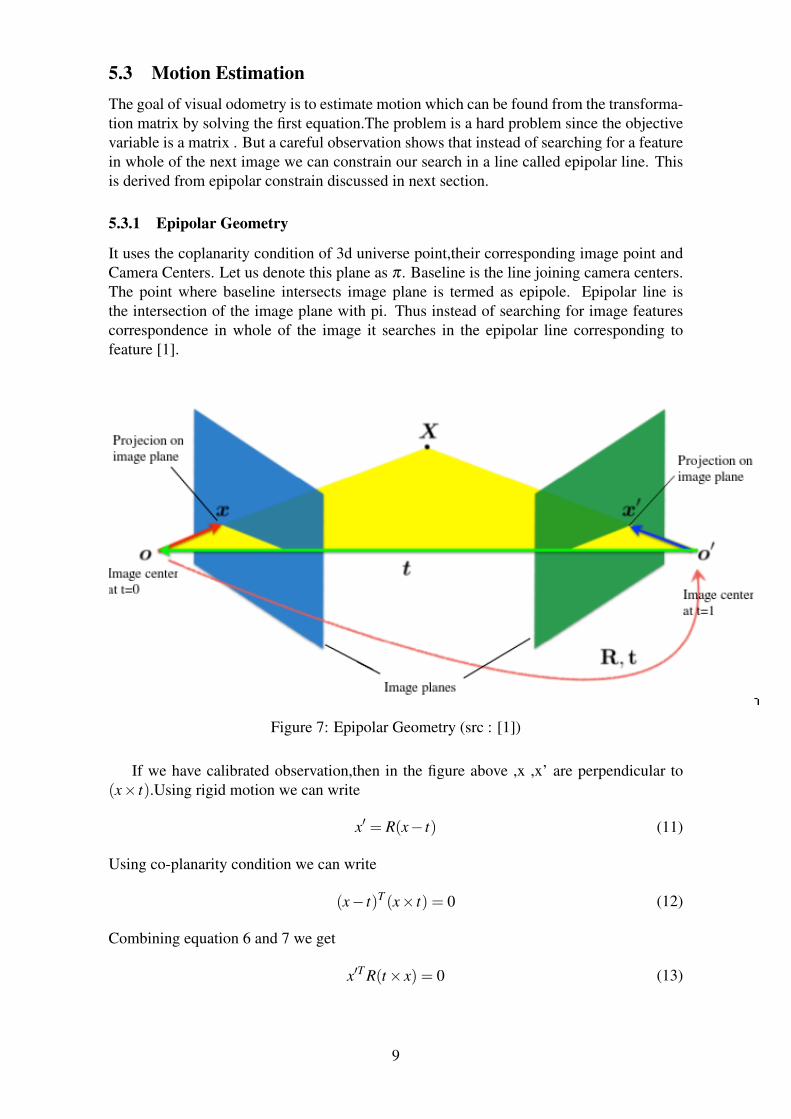
It uses the coplanarity condition of 3d universe point,their corresponding image point andCamera Centers. Let us denote this plane as π . Baseline is the line joining camera centers.The point where baseline intersects image plane is termed as epipole. Epipolar line isthe intersection of the image plane with pi. Thus instead of searching for image featurescorrespondence in whole of the image it searches in the epipolar line corresponding tofeature [1].

Figure 7: Epipolar Geometry (src : [1])

If we have calibrated observation,then in the figure above ,x ,x’ are perpendicular to(x× t).Using rigid motion we can write

x′ = R(x− t) (11)

Using co-planarity condition we can write

(x− t)T (x× t) = 0 (12)

Combining equation 6 and 7 we get

x′T R(t× x) = 0 (13)

9

To represent cross-product in matrix form, (t× x) is represented as [tx]x where

[tx] =

0 −t3 t2t3 0 −t1−t2 t1 0

Thereforex′T R(t× x) = 0 (15)

x′T Ex = 0 (16)

Where E =R[tx] is called essential matrix.

5.3.2 Essential matrix computation

As discussed above once we have x and x′, we can calculate essential Matrix E which sat-

isfies equation(11). An essential matrix can be computed using Nister’s 5 point algorithm.Equation (11) can be re-written as:

xT E = 0 (17)

wherex = [x1x

′1 x2x

′1 x3x

′1 x1x

′2 x2x

′2 x3x

′2 x1x

′3 x2x

′3 x3x

′3]

T (18)

E = [E11 E12 E13 E21 E22 E23 E31 E32 E33] (19)

As there are five unknowns in E matrix (3 angles and 2 translation elements), we stackfive such x points and form a 5× 9 matrix (say X). Nister[5] proposed a mathematicalsolution for the equation

XT E = 0 (20)

which gives the solution matrix E. It requires minimal 5 points which is better than previ-ous 8 point algorithm. It involves calculating coefficients and finding roots of 10th orderpolynomials. But from feature tracking we have so many pairs of points (x and x

′) which

may also contain some outliers (due to least squares solution described above). So, weneed to choose a set of 5 pairs from them. This selection is done using RANSAC.

• RANSAC : Feature correspondences using KLT tracker are often erroneous and therecan be outliers. Least squares fitting uses all of the data and can be influenced byoutliers. In order to have better feature correspondence, we uses iterative RandomSample Consensus, abbreviated as RANSAC [3], to remove outliers. At each itera-tion RANSAC uniformly selects a subset of data samples and then Essential matrixis computed. It checks if this essential matrix satisfies the equation (15) for all pointpairs. The pairs which satisfies equation(15) are called inliers. RANSAC terminatesif the count of the inliers is higher than specified amount by user. If the number issatisfied then it returns this matrix as final Essential matrix, otherwise it searches forpoints once again until it reaches maximum number of loops specified by the user.

10

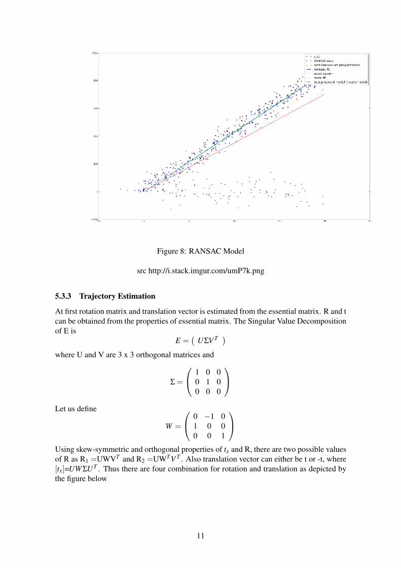
Figure 8: RANSAC Model

src http://i.stack.imgur.com/umP7k.png

5.3.3 Trajectory Estimation

At first rotation matrix and translation vector is estimated from the essential matrix. R and tcan be obtained from the properties of essential matrix. The Singular Value Decompositionof E is

E =(

UΣV T )where U and V are 3 x 3 orthogonal matrices and

Σ =

1 0 00 1 00 0 0

Let us define

W =

0 −1 01 0 00 0 1

Using skew-symmetric and orthogonal properties of tx and R, there are two possible valuesof R as R1 =UWVT and R2 =UWTV T . Also translation vector can either be t or -t, where[tx]=UWΣUT . Thus there are four combination for rotation and translation as depicted bythe figure below

11

Figure 9: Four Solutions

src: http://isit.u-clermont1.fr/ ab/Classes/DIKU-3DCV2/Handouts/Lecture16.pdf

The t and -t swaps the position of the cameras. R1 and R2 makes a rotation of pi aroundthe baseline. Therefore only one solution is feasible which is obtained via triangulation of apoint and choosing the solution where the point is in front of both cameras. This conditionis called cheirality constraint [4]. After estimating R and t, the trajectory is obtained by theequation:

tnew = told + scale.RnewtRnew = R.Rold

• Scale Ambiguity There are multiple solutions for t as many possible decompositionof E and consecutively different set of U and Σ. Therefore scale ambiguity remainsproblem for a monocular system. We can use I.M.U. sensor data to resolve the prob-lem.

6 Experiments and Results

6.1 DatasetWe are training our algorithm on images obtained from Ford Campus Vision and LIDARDataset [6] which were taken in an urban environment. The dataset was collected by anautonomous ground vehicle testbed, based upon a modified Ford F-250 pickup truck. Theimages were captured at the rate of 8fps so that we have sufficient overlap over images.The camera was mounted laterally on the car to get a wider environmental view.

12

6.2 Experimental SetupThe images obtained were adjusted for distortion. The images had a part of vehicle whichresulted in considerable feature points detected on that part of vehicle. So we cropped theimage to remove the unnecessary parts to ensure correct transformation matrix. This crop-ping doesn’t effect the focal parameters but the principal point should be translated by theamount of cropping done.As explained above, the images obtained were rotated 90◦ anticlockwise from actual straightview.(sample image to be attached). Since the axis of the vehicle doesn’t align with the ro-tated camera we rotated the given image to align with the vehicle’s axis. This resulted inchanged intrinsic parameters which were computed by the following equations: If h and ware height and width of the images then for the rotated images principal point cx,cy for newrotated images are given by

xnew = h− yold

ynew = xold

6.3 ResultsThe ground truth for the dataset is:

Figure 10: Ground truth of the trajectory

Tracking path using FAST feature detector and KLT tracker

13

Figure 11: Estimated trajectory using FAST Detector

We also tracked using SIFT feature detector and KLT tracker:

Figure 12: Estimated Trajectory using SIFT Feature Detector

The sampled points by FAST feature detector are :

14

Figure 13: Fast Detectors

Results of KLT tracker is below:

Figure 14: KLT Tracker

7 DiscussionWe implemented the monocular visual odometry on Ford Campus Vision and LIDARDataset. We observed that when vehicle moves straight, our program generates straightpath but it is tilted as shown above. This is due to the fact that we are calculating trans-formations relatively in visual odometry.This can be rectified using information from IMUsensors(not necessarily costly) or LIDAR sensors. The results using FAST were satisfac-tory. There is also a slight error in path prediction due to incorrect scale. This can be alsobe solved by IMU data or Bundle Adjustment. Results using sift are also satisfactory butSIFT took more time than FAST in feature detection step.

15

8 Conclusions and Future workIn general as tasks involving visual odometry needs to be ran in real time, we thus considerimplementing FAST in our main work.

• Resolving Scale Ambiguity:We hope to resolve the scale ambiguity and tilt in thepath using . We are trying to implement kalman filter which also takes other sensordata apart from camera images (I.M.U.) in our case.

• Another way of solving the scale ambiguity is to use Bundle Adjustment(BA) whichfinds scale by triangulating 3D points using previous frames and then re-projectingthe points back to image to find scale factor for current timestamp. We would like touse this to resolve scale ambiguity as it helps in reducing the use of IMU’s.

9 AcknowledgementWe thank Prof. Gaurav Pandey, Dept. of Electrical Engineering for his valuable supportthroughout the project guiding us from time to time and looking into the project when itwas needed. We also thank OpenCV community for their user friendly libraries.

References[1] Epipolar Geometry. http://www.cs.cmu.edu/~16385/lectures/Lecture18.

pdf.

[2] HighSpeed Test for Fast opencv documentation. http://docs.opencv.org/3.

0-beta/doc/py_tutorials/py_feature2d/py_fast/py_fast.html.

[3] RANSAC Tutorial. http://image.ing.bth.se/ipl-bth/siamak.khatibi/

AIPBTH13LP2/lectures/RANSAC-tutorial.pdf.

[4] LOWE, D. G. Distinctive image features from scale-invariant keypoints. Internationaljournal of computer vision 60, 2 (2004), 91–110.

[5] NISTER, D. An efficient solution to the five-point relative pose problem. PatternAnalysis and Machine Intelligence, IEEE Transactions on 26, 6 (2004), 756–770.

[6] PANDEY, G., MCBRIDE, J. R., AND EUSTICE, R. M. Ford campus vision and lidardata set. International Journal of Robotics Research 30, 13 (2011), 1543–1552.

[7] ROSTEN, E., PORTER, R., AND DRUMMOND, T. Faster and better: A machine learn-ing approach to corner detection. IEEE Trans. Pattern Analysis and Machine Intelli-gence 32 (2010), 105–119.

[8] SCARAMUZZA, D., AND FRAUNDORFER, F. Visual odometry [tutorial]. Robotics &Automation Magazine, IEEE 18, 4 (2011), 80–92.

[9] TOMASI, C., AND KANADE, T. Detection and tracking of point features. School ofComputer Science, Carnegie Mellon Univ. Pittsburgh, 1991.

16