visual control of robots: - peter corke
TRANSCRIPT

VISUAL CONTROLOFROBOTS:
High-PerformanceVisual Servoing
PeterI. CorkeCSIRO Divisionof ManufacturingTechnology, Australia.

To my family, Phillipa,Lucy andMadeline.
v

vi

Editorial foreword
It is no longernecessaryto explain theword 'mechatronics'.Theworld hasbecomeaccustomedto theblendingof mechanics,electronicsandcomputercontrol.Thatdoesnot meanthatmechatronicshaslost its 'art'.
Theadditionof vision sensingto assistin thesolutionof a varietyof problemsisstill very mucha 'cutting edge'topicof research.PeterCorkehaswrittena veryclearexpositionwhichembracesboththetheoryandthepracticalproblemsencounteredinaddingvisionsensingto a robotarm.
Thereis greatvaluein thisbook,bothfor advancedundergraduatereadingandfortheresearcheror designerin industrywhowishesto addvision-basedcontrol.
We will onedaycometo expectvisionsensingandcontrol to bea regularfeatureof mechatronicdevicesfrom machinetoolsto domesticappliances.It is researchsuchasthiswhichwill bring thatdayabout.
JohnBillingsleyUniversityof SouthernQueensland,
Toowoomba,QLD4350August1996
vii

viii

Author' sPreface
Outline
This book is abouttheapplicationof high-speedmachinevision for closed-looppo-sition control,or visual servoing, of a robot manipulator. The bookaimsto providea comprehensive coverageof all aspectsof thevisualservoing problem:robotics,vi-sion, control, technologyandimplementationissues.While muchof the discussionis quitegeneraltheexperimentalwork describedis basedon theuseof a high-speedbinaryvisionsystemwith a monocular'eye-in-hand'camera.
Theparticularfocusis onaccuratehigh-speedmotion,wherein thiscontext 'highspeed'is takento meanapproaching,or exceeding,theperformancelimits statedbythe robot manufacturer. In orderto achieve suchhigh-performanceI arguethat it isnecessaryto haveaccuratedynamicalmodelsof thesystemto becontrolled(therobot)andthesensor(thecameraandvisionsystem).Despitethelonghistoryof researchintheconstituenttopicsof roboticsandcomputervision,thesystemdynamicsof closed-loop visually guidedrobot systemshasnot beenwell addressedin the literaturetodate.
I am a confirmedexperimentalistandthereforethis book hasa strongthemeofexperimentation. Experimentsareusedto build and verify modelsof the physicalsystemcomponentssuchasrobots,camerasandvision systems.Thesemodelsarethenusedfor controllersynthesis,andthecontrollersareverifiedexperimentallyandcomparedwith resultsobtainedby simulation.
Finally, the book hasa World Wide Web homepagewhich serves as a virtualappendix.It containslinks to thesoftwareandmodelsdiscussedwithin thebookaswell aspointersto otherusefulsourcesof information. A videotape,showing manyof theexperiments,canbeorderedvia thehomepage.
Background
My interestin theareaof visualservoing datesbackto 1984whenI wasinvolvedintwo researchprojects;video-ratefeatureextraction1, andsensor-basedrobotcontrol.At that time it becameapparentthat machinevision could be usedfor closed-loopcontrol of robot position, sincethe video-field rate of 50Hz exceededthe positionsetpointrateof thePumarobotwhich is only 36Hz. AroundthesameperiodWeissandSandersonpublishedanumberof papersonthis topic[224–226,273]in particularconcentratingon control strategiesandthe direct useof imagefeatures— but onlyin simulation. I was interestedin actuallybuilding a systembasedon the feature-extractorandrobotcontroller, but for anumberof reasonsthiswasnotpossibleat thattime.
1This work resultedin a commercialunit — theAPA-512 [261], andits successortheAPA-512+ [25].Bothdevicesaremanufacturedby AtlantekMicrosystemsLtd. of Adelaide,Australia.
ix

In the period1988–89I wasfortunatein beingable to spend11 monthsat theGRASPLaboratory, University of Pennsylvaniaon a CSIRO OverseasFellowship.ThereI was able to demonstratea 60Hz visual feedbacksystem[65]. Whilst thesampleratewashigh, theactualclosed-loopbandwidthwasquite low. Clearly therewasa needto morecloselymodel the systemdynamicsso as to be ableto achievebettercontrolperformance.Onreturnto Australiathisbecamethesubjectof my PhDresearch[52].
Nomenclature
Themostcommonlyusedsymbolsusedin this book,andtheir unitsarelistedbelow.Note thatsomesymbolsareoverloadedin which casetheir context mustbeusedtodisambiguatethem.
v a vectorvx a componentof a vectorA a matrixx anestimateof xx errorin xxd demandedvalueof xAT transposeof Aαx, αy pixel pitch pixels/mmB viscousfriction coefficient N m s radC cameracalibrationmatrix (3 4)C q q manipulatorcentripetalandCoriolis term kg m2 sceil x returnsn, thesmallestintegersuchthatn xE illuminance(lux) lxf force Nf focal length mF f -numberF q friction torque N.mfloor x returnsn, thelargestintegersuchthatn xG gearratioφ luminousflux (lumens) lmφ magneticflux (Webers) WbG gearratiomatrixG q manipulatorgravity loadingterm N.mi current AIn n n identitymatrixj 1J scalarinertia kg m2
x

J inertiatensor, 3 3 matrix kg m2
AJB Jacobiantransformingvelocitiesin frameA to frameBk K constantKi amplifiergain(transconductance) A/VKm motortorqueconstant N.m/AK forwardkinematicsK 1 inversekinematicsL inductance HL luminance(nit) ntmi massof link i kgM q manipulatorinertiamatrix kg m2
Ord orderof polynomialq generalizedjoint coordinatesQ generalizedjoint torque/forceR resistance Ωθ angle radθ vectorof angles,generallyrobotjoint angles rads Laplacetransformoperatorsi COM of link i with respectto thelink i coordinateframe mSi first momentof link i. Si misi kg.mσ standarddeviationt time sT sampleinterval sT lenstransmissionconstantTe cameraexposureinterval sT homogeneoustransformationATB homogeneoustransformof point B with respectto the
frameA. If A is notgiventhenassumedrelative to worldcoordinateframe0. NotethatATB
BTA1.
τ torque N.mτC Coulombfriction torque N.mv voltage Vω frequency rad sx 3-D pose, x x y z rx ry rz
T comprising translationalong,androtationabouttheX, Y andZ axes.
x y z CartesiancoordinatesX0, Y0 coordinatesof theprincipalpoint pixelsix iy cameraimageplanecoordinates miX iY cameraimageplanecoordinates pixelsiX cameraimageplanecoordinatesiX iX iY pixelsi X imageplaneerror
xi

z z-transformoperatorZ Z-transform
Thefollowing conventionshave alsobeenadopted:
Timedomainvariablesarein lowercase,frequency domainin uppercase.
Transferfunctionswill frequentlybewrittenusingthenotation
K a ζ ωn Ksa
11
ω2ns2 2ζ
ωns 1
A freeintegratoris anexception,and 0 is usedto represents.
Whenspecifyingmotor motion, inertiaandfriction parametersit is importantthataconsistentreferenceis used,usuallyeitherthemotoror theload,denotedby thesubscriptsm or l respectively.
For numericquantitiestheunits radmandradlareusedto indicatethereferenceframe.
In orderto clearlydistinguishresultsthatwereexperimentallydeterminedfromsimulatedor derivedresults,theformerwill alwaysbedesignatedas'measured'in thecaptionandindex entry.
A comprehensive glossaryof termsandabbreviationsis providedin AppendixA.
xii

Acknowledgements
Thework describedin this bookis largelybasedonmy PhDresearch[52] whichwascarriedout, part time, at the Universityof Melbourneover the period1991–94.MysupervisorsProfessorMalcolm Goodat the University of Melbourne,andDr. PaulDunnat CSIRO providedmuchvaluablediscussionandguidanceover thecourseoftheresearch,andcritical commentson thedraft text.
Thatwork couldnot have occurredwithout thegenerosityandsupportof my em-ployer, CSIRO. I am indebtedto Dr. Bob Brown andDr. S. Ramakrishnanfor sup-portingmein theOverseasFellowshipandPhDstudy, andmakingavailablethenec-essarytime andlaboratoryfacilities. I would like to thankmy CSIRO colleaguesfortheir supportof this work, in particular:Dr. Paul Dunn,Dr. Patrick Kearney, RobinKirkham,DennisMills, andVaughanRobertsfor technicaladviceandmuchvaluablediscussion;Murray JensenandGeoff Lamb for keepingthe computersystemsrun-ning; JannisYoungandKaryn Gee,the librarians,for trackingdown all mannerofreferences;Les Ewbankfor mechanicaldesignanddrafting; Ian Brittle' s ResearchSupportGroupfor mechanicalconstruction;andTerry Harvey andSteve Hoganforelectronicconstruction. The PhD work was partially supportedby a University ofMelbourne/ARCsmall grant. Writing this bookwaspartially supportedby the Co-operative ResearchCentrefor Mining TechnologyandEquipment(CMTE), a jointventurebetweenAMIRA, CSIRO, andtheUniversityof Queensland.
Many othershelpedaswell. ProfessorRichard(Lou) Paul, Universityof Penn-sylvania, was thereat the beginning and madefacilities at the GRASPlaboratoryavailableto me.Dr. Kim Ng of MonashUniversityandDr. Rick Alexanderhelpedindiscussionsoncameracalibrationandlensdistortion,andalsoloanedmetheSHAPEsystemcalibrationtargetusedin Chapter4. VisionSystemsLtd. of Adelaide,throughtheir thenUSdistributorTom Seitzlerof Vision International,loanedmeanAPA-512video-ratefeatureextractorunit for usewhile I wasat theGRASPLaboratory. DavidHoadley proofreadtheoriginalthesis,andmy next doorneighbour, JackDavies,fixedlots of thingsaroundmy housethatI didn't getaroundto doing.
xiii

xiv

Contents
1 Intr oduction 11.1 Visualservoing . . . . . . . . . . . . . . . . . . . . . . . . . . . . . 1
1.1.1 Relateddisciplines . . . . . . . . . . . . . . . . . . . . . . . 51.2 Structureof thebook . . . . . . . . . . . . . . . . . . . . . . . . . . 5
2 Modelling the robot 72.1 Manipulatorkinematics. . . . . . . . . . . . . . . . . . . . . . . . . 7
2.1.1 Forwardandinversekinematics . . . . . . . . . . . . . . . . 102.1.2 Accuracy andrepeatability. . . . . . . . . . . . . . . . . . . 112.1.3 Manipulatorkinematicparameters. . . . . . . . . . . . . . . 12
2.2 Manipulatorrigid-bodydynamics . . . . . . . . . . . . . . . . . . . 142.2.1 RecursiveNewton-Eulerformulation . . . . . . . . . . . . . 162.2.2 Symbolicmanipulation. . . . . . . . . . . . . . . . . . . . . 192.2.3 Forwarddynamics . . . . . . . . . . . . . . . . . . . . . . . 212.2.4 Rigid-bodyinertialparameters. . . . . . . . . . . . . . . . . 212.2.5 Transmissionandgearing . . . . . . . . . . . . . . . . . . . 272.2.6 Quantifyingrigid bodyeffects . . . . . . . . . . . . . . . . . 282.2.7 Robotpayload . . . . . . . . . . . . . . . . . . . . . . . . . 30
2.3 Electro-mechanicaldynamics. . . . . . . . . . . . . . . . . . . . . . 312.3.1 Friction . . . . . . . . . . . . . . . . . . . . . . . . . . . . . 322.3.2 Motor . . . . . . . . . . . . . . . . . . . . . . . . . . . . . . 352.3.3 Currentloop . . . . . . . . . . . . . . . . . . . . . . . . . . 422.3.4 Combinedmotorandcurrent-loopdynamics . . . . . . . . . 452.3.5 Velocity loop . . . . . . . . . . . . . . . . . . . . . . . . . . 492.3.6 Positionloop . . . . . . . . . . . . . . . . . . . . . . . . . . 522.3.7 Fundamentalperformancelimits . . . . . . . . . . . . . . . . 56
2.4 Significanceof dynamiceffects. . . . . . . . . . . . . . . . . . . . . 582.5 Manipulatorcontrol . . . . . . . . . . . . . . . . . . . . . . . . . . . 60
2.5.1 Rigid-bodydynamicscompensation. . . . . . . . . . . . . . 60
xv

xvi CONTENTS
2.5.2 Electro-mechanicaldynamicscompensation. . . . . . . . . . 642.6 Computationalissues . . . . . . . . . . . . . . . . . . . . . . . . . . 64
2.6.1 Parallelcomputation . . . . . . . . . . . . . . . . . . . . . . 652.6.2 Symbolicsimplificationof run-timeequations. . . . . . . . . 662.6.3 Significance-basedsimplification . . . . . . . . . . . . . . . 672.6.4 Comparison. . . . . . . . . . . . . . . . . . . . . . . . . . . 68
3 Fundamentalsof imagecapture 733.1 Light . . . . . . . . . . . . . . . . . . . . . . . . . . . . . . . . . . . 73
3.1.1 Illumination . . . . . . . . . . . . . . . . . . . . . . . . . . . 733.1.2 Surfacereflectance. . . . . . . . . . . . . . . . . . . . . . . 753.1.3 Spectralcharacteristicsandcolor temperature. . . . . . . . . 76
3.2 Imageformation. . . . . . . . . . . . . . . . . . . . . . . . . . . . . 793.2.1 Light gatheringandmetering. . . . . . . . . . . . . . . . . . 813.2.2 Focusanddepthof field . . . . . . . . . . . . . . . . . . . . 823.2.3 Imagequality . . . . . . . . . . . . . . . . . . . . . . . . . . 843.2.4 Perspective transform. . . . . . . . . . . . . . . . . . . . . . 86
3.3 Cameraandsensortechnologies . . . . . . . . . . . . . . . . . . . . 873.3.1 Sensors. . . . . . . . . . . . . . . . . . . . . . . . . . . . . 883.3.2 Spatialsampling . . . . . . . . . . . . . . . . . . . . . . . . 913.3.3 CCDexposurecontrolandmotionblur . . . . . . . . . . . . 943.3.4 Linearity . . . . . . . . . . . . . . . . . . . . . . . . . . . . 953.3.5 Sensitivity . . . . . . . . . . . . . . . . . . . . . . . . . . . 963.3.6 Darkcurrent . . . . . . . . . . . . . . . . . . . . . . . . . . 1003.3.7 Noise . . . . . . . . . . . . . . . . . . . . . . . . . . . . . . 1003.3.8 Dynamicrange . . . . . . . . . . . . . . . . . . . . . . . . . 102
3.4 Videostandards. . . . . . . . . . . . . . . . . . . . . . . . . . . . . 1023.4.1 Interlacingandmachinevision . . . . . . . . . . . . . . . . . 105
3.5 Imagedigitization . . . . . . . . . . . . . . . . . . . . . . . . . . . . 1063.5.1 OffsetandDC restoration . . . . . . . . . . . . . . . . . . . 1073.5.2 Signalconditioning. . . . . . . . . . . . . . . . . . . . . . . 1073.5.3 Samplingandaspectratio . . . . . . . . . . . . . . . . . . . 1073.5.4 Quantization . . . . . . . . . . . . . . . . . . . . . . . . . . 1123.5.5 OverallMTF . . . . . . . . . . . . . . . . . . . . . . . . . . 1133.5.6 Visualtemporalsampling . . . . . . . . . . . . . . . . . . . 115
3.6 Cameraandlighting constraints . . . . . . . . . . . . . . . . . . . . 1163.6.1 Illumination . . . . . . . . . . . . . . . . . . . . . . . . . . . 118
3.7 Thehumaneye . . . . . . . . . . . . . . . . . . . . . . . . . . . . . 121

CONTENTS xvii
4 Machine vision 1234.1 Imagefeatureextraction . . . . . . . . . . . . . . . . . . . . . . . . 123
4.1.1 Wholescenesegmentation . . . . . . . . . . . . . . . . . . . 1244.1.2 Momentfeatures . . . . . . . . . . . . . . . . . . . . . . . . 1274.1.3 Binaryregion features . . . . . . . . . . . . . . . . . . . . . 1304.1.4 Featuretracking . . . . . . . . . . . . . . . . . . . . . . . . 136
4.2 Perspective andphotogrammetry. . . . . . . . . . . . . . . . . . . . 1374.2.1 Close-rangephotogrammetry. . . . . . . . . . . . . . . . . . 1384.2.2 Cameracalibrationtechniques. . . . . . . . . . . . . . . . . 1394.2.3 Eye-handcalibration . . . . . . . . . . . . . . . . . . . . . . 147
5 Visual servoing 1515.1 Fundamentals. . . . . . . . . . . . . . . . . . . . . . . . . . . . . . 1525.2 Priorwork . . . . . . . . . . . . . . . . . . . . . . . . . . . . . . . . 1545.3 Position-basedvisualservoing . . . . . . . . . . . . . . . . . . . . . 159
5.3.1 Photogrammetrictechniques. . . . . . . . . . . . . . . . . . 1595.3.2 Stereovision . . . . . . . . . . . . . . . . . . . . . . . . . . 1605.3.3 Depthfrom motion . . . . . . . . . . . . . . . . . . . . . . . 160
5.4 Imagebasedservoing . . . . . . . . . . . . . . . . . . . . . . . . . . 1615.4.1 Approachesto image-basedvisualservoing . . . . . . . . . . 163
5.5 Implementationissues . . . . . . . . . . . . . . . . . . . . . . . . . 1665.5.1 Cameras. . . . . . . . . . . . . . . . . . . . . . . . . . . . . 1665.5.2 Imageprocessing. . . . . . . . . . . . . . . . . . . . . . . . 1675.5.3 Featureextraction. . . . . . . . . . . . . . . . . . . . . . . . 1675.5.4 Visualtaskspecification . . . . . . . . . . . . . . . . . . . . 169
6 Modelling an experimentalvisual servosystem 1716.1 Architecturesanddynamicperformance. . . . . . . . . . . . . . . . 1726.2 Experimentalhardwareandsoftware. . . . . . . . . . . . . . . . . . 175
6.2.1 Processorandoperatingsystem . . . . . . . . . . . . . . . . 1766.2.2 Robotcontrolhardware. . . . . . . . . . . . . . . . . . . . . 1776.2.3 ARCL . . . . . . . . . . . . . . . . . . . . . . . . . . . . . . 1786.2.4 Visionsystem. . . . . . . . . . . . . . . . . . . . . . . . . . 1796.2.5 Visualservo supportsoftware— RTVL . . . . . . . . . . . . 182
6.3 Kinematicsof cameramountandlens . . . . . . . . . . . . . . . . . 1846.3.1 Cameramountkinematics . . . . . . . . . . . . . . . . . . . 1846.3.2 Modellingthelens . . . . . . . . . . . . . . . . . . . . . . . 188
6.4 Visualfeedbackcontrol . . . . . . . . . . . . . . . . . . . . . . . . . 1916.4.1 Controlstructure . . . . . . . . . . . . . . . . . . . . . . . . 1946.4.2 “Black box” experiments. . . . . . . . . . . . . . . . . . . . 1956.4.3 Modellingsystemdynamics . . . . . . . . . . . . . . . . . . 197
xviii CONTENTS
6.4.4 Theeffectof multi-ratesampling . . . . . . . . . . . . . . . 2016.4.5 A single-ratemodel. . . . . . . . . . . . . . . . . . . . . . . 2036.4.6 Theeffectof camerashutterinterval . . . . . . . . . . . . . . 2046.4.7 Theeffectof targetrange. . . . . . . . . . . . . . . . . . . . 2066.4.8 Comparisonwith joint controlschemes . . . . . . . . . . . . 2086.4.9 Summary . . . . . . . . . . . . . . . . . . . . . . . . . . . . 209
7 Control designand performance 2117.1 Controlformulation . . . . . . . . . . . . . . . . . . . . . . . . . . . 2127.2 Performancemetrics . . . . . . . . . . . . . . . . . . . . . . . . . . 2147.3 Compensatordesignandevaluation . . . . . . . . . . . . . . . . . . 215
7.3.1 Addition of anextra integrator . . . . . . . . . . . . . . . . . 2157.3.2 PID controller. . . . . . . . . . . . . . . . . . . . . . . . . . 2167.3.3 Smith'smethod. . . . . . . . . . . . . . . . . . . . . . . . . 2187.3.4 Statefeedbackcontrollerwith integralaction . . . . . . . . . 2197.3.5 Summary . . . . . . . . . . . . . . . . . . . . . . . . . . . . 225
7.4 Axis controlmodesfor visualservoing . . . . . . . . . . . . . . . . . 2277.4.1 Torquecontrol . . . . . . . . . . . . . . . . . . . . . . . . . 2287.4.2 Velocitycontrol . . . . . . . . . . . . . . . . . . . . . . . . . 2297.4.3 Positioncontrol . . . . . . . . . . . . . . . . . . . . . . . . . 2317.4.4 Discussion . . . . . . . . . . . . . . . . . . . . . . . . . . . 2317.4.5 Non-linearsimulationandmodelerror . . . . . . . . . . . . . 2337.4.6 Summary . . . . . . . . . . . . . . . . . . . . . . . . . . . . 234
7.5 Visualfeedforwardcontrol . . . . . . . . . . . . . . . . . . . . . . . 2357.5.1 High-performanceaxisvelocitycontrol . . . . . . . . . . . . 2377.5.2 Targetstateestimation . . . . . . . . . . . . . . . . . . . . . 2427.5.3 Feedforwardcontrolimplementation. . . . . . . . . . . . . . 2517.5.4 Experimentalresults . . . . . . . . . . . . . . . . . . . . . . 255
7.6 Biologicalparallels . . . . . . . . . . . . . . . . . . . . . . . . . . . 2577.7 Summary . . . . . . . . . . . . . . . . . . . . . . . . . . . . . . . . 260
8 Further experimentsin visual servoing 2638.1 Visualcontrolof a majoraxis . . . . . . . . . . . . . . . . . . . . . . 263
8.1.1 Theexperimentalsetup. . . . . . . . . . . . . . . . . . . . . 2648.1.2 Trajectorygeneration. . . . . . . . . . . . . . . . . . . . . . 2658.1.3 Puma'native' positioncontrol . . . . . . . . . . . . . . . . . 2668.1.4 Understandingjoint 1 dynamics . . . . . . . . . . . . . . . . 2698.1.5 Single-axiscomputedtorquecontrol . . . . . . . . . . . . . . 2748.1.6 Visionbasedcontrol . . . . . . . . . . . . . . . . . . . . . . 2798.1.7 Discussion . . . . . . . . . . . . . . . . . . . . . . . . . . . 281
8.2 High-performance3D translationalvisualservoing . . . . . . . . . . 282

CONTENTS xix
8.2.1 Visualcontrolstrategy . . . . . . . . . . . . . . . . . . . . . 2838.2.2 Axis velocitycontrol . . . . . . . . . . . . . . . . . . . . . . 2868.2.3 Implementationdetails . . . . . . . . . . . . . . . . . . . . . 2878.2.4 Resultsanddiscussion . . . . . . . . . . . . . . . . . . . . . 290
8.3 Conclusion . . . . . . . . . . . . . . . . . . . . . . . . . . . . . . . 294
9 Discussionand futur e dir ections 2979.1 Discussion. . . . . . . . . . . . . . . . . . . . . . . . . . . . . . . . 2979.2 Visualservoing: somequestions(andanswers) . . . . . . . . . . . . 2999.3 Futurework . . . . . . . . . . . . . . . . . . . . . . . . . . . . . . . 302
Bibliography 303
A Glossary 321
B This book on the Web 325
C APA-512 327
D RTVL: a software systemfor robot visual servoing 333D.1 Imageprocessingcontrol . . . . . . . . . . . . . . . . . . . . . . . . 334D.2 Imagefeatures. . . . . . . . . . . . . . . . . . . . . . . . . . . . . . 334D.3 Timestampsandsynchronizedinterrupts . . . . . . . . . . . . . . . 335D.4 Real-timegraphics . . . . . . . . . . . . . . . . . . . . . . . . . . . 337D.5 Variablewatch . . . . . . . . . . . . . . . . . . . . . . . . . . . . . 337D.6 Parameters. . . . . . . . . . . . . . . . . . . . . . . . . . . . . . . . 338D.7 Interactivecontrolfacility . . . . . . . . . . . . . . . . . . . . . . . . 338D.8 Datalogginganddebugging . . . . . . . . . . . . . . . . . . . . . . 338D.9 Robotcontrol . . . . . . . . . . . . . . . . . . . . . . . . . . . . . . 340D.10 Applicationprogramfacilities . . . . . . . . . . . . . . . . . . . . . 340D.11 An example— planarpositioning . . . . . . . . . . . . . . . . . . . 340D.12 Conclusion . . . . . . . . . . . . . . . . . . . . . . . . . . . . . . . 341
E LED strobe 343
Index 347

xx CONTENTS

List of Figures
1.1 Generalstructureof hierarchicalmodel-basedrobotandvisionsystem. 4
2.1 Dif ferentformsof Denavit-Hartenberg notation. . . . . . . . . . . . . 82.2 Detailsof coordinateframesusedfor Puma560 . . . . . . . . . . . . 132.3 Notationfor inversedynamics . . . . . . . . . . . . . . . . . . . . . 172.4 Measuredandestimatedgravity loadon joint 2. . . . . . . . . . . . . 252.5 Configurationdependentinertiafor joint 1 . . . . . . . . . . . . . . . 292.6 Configurationdependentinertiafor joint 2 . . . . . . . . . . . . . . . 292.7 Gravity loadon joint 2 . . . . . . . . . . . . . . . . . . . . . . . . . 302.8 Typical friction versusspeedcharacteristic. . . . . . . . . . . . . . . 322.9 Measuredmotorcurrentversusjoint velocity for joint 2 . . . . . . . . 342.10 Block diagramof motormechanicaldynamics. . . . . . . . . . . . . 362.11 Schematicof motorelectricalmodel. . . . . . . . . . . . . . . . . . . 362.12 Measuredjoint angleandvoltagedatafrom open-circuitteston joint 2. 392.13 Block diagramof motorcurrentloop . . . . . . . . . . . . . . . . . . 432.14 Measuredjoint 6 current-loopfrequency response. . . . . . . . . . . 442.15 Measuredjoint 6 motorandcurrent-looptransferfunction. . . . . . . 452.16 Measuredmaximumcurrentstepresponsefor joint 6. . . . . . . . . . 482.17 SIMULINK modelMOTOR . . . . . . . . . . . . . . . . . . . . . . 502.18 SIMULINK modelLMOTOR . . . . . . . . . . . . . . . . . . . . . 502.19 Velocity loopblockdiagram. . . . . . . . . . . . . . . . . . . . . . . 512.20 Measuredjoint 6 velocity-looptransferfunction . . . . . . . . . . . . 522.21 SIMULINK modelVLOOP . . . . . . . . . . . . . . . . . . . . . . 522.22 Unimationservo positioncontrolmode. . . . . . . . . . . . . . . . . 532.23 Block diagramof Unimationpositioncontrolloop. . . . . . . . . . . 542.24 Root-locusdiagramof positionloopwith no integralaction. . . . . . 562.25 Root-locusdiagramof positionloopwith integralactionenabled.. . . 562.26 SIMULINK modelPOSLOOP . . . . . . . . . . . . . . . . . . . . . 572.27 Unimationservo currentcontrolmode.. . . . . . . . . . . . . . . . . 572.28 Standardtrajectorytorquecomponents. . . . . . . . . . . . . . . . . 59
xxi
xxii LIST OF FIGURES
2.29 Computedtorquecontrolstructure.. . . . . . . . . . . . . . . . . . . 612.30 Feedforwardcontrolstructure. . . . . . . . . . . . . . . . . . . . . . 612.31 Histogramof torqueexpressioncoefficient magnitudes . . . . . . . . 68
3.1 Stepsinvolvedin imageprocessing. . . . . . . . . . . . . . . . . . . 743.2 Luminositycurve for standardobserver. . . . . . . . . . . . . . . . . 753.3 Specularanddiffusesurfacereflectance . . . . . . . . . . . . . . . . 763.4 Blackbodyemissionsfor solarandtungstenillumination. . . . . . . . 773.5 Elementaryimageformation . . . . . . . . . . . . . . . . . . . . . . 793.6 Depthof field bounds. . . . . . . . . . . . . . . . . . . . . . . . . . 833.7 Centralperspective geometry. . . . . . . . . . . . . . . . . . . . . . . 873.8 CCDphotositechargewellsandincidentphotons.. . . . . . . . . . . 883.9 CCDsensorarchitectures. . . . . . . . . . . . . . . . . . . . . . . . 893.10 Pixel exposureintervals . . . . . . . . . . . . . . . . . . . . . . . . . 913.11 Cameraspatialsampling . . . . . . . . . . . . . . . . . . . . . . . . 923.12 Somephotositecaptureprofiles. . . . . . . . . . . . . . . . . . . . . 933.13 MTF for variouscaptureprofiles. . . . . . . . . . . . . . . . . . . . . 933.14 Exposureinterval of thePulnixcamera. . . . . . . . . . . . . . . . . 953.15 Experimentalsetupto determinecamerasensitivity. . . . . . . . . . . 973.16 Measuredresponseof AGCcircuit to changingillumination. . . . . . 983.17 Measuredresponseof AGCcircuit to stepilluminationchange.. . . . 993.18 Measuredspatialvarianceof illuminanceasa functionof illuminance. 1023.19 CCIRstandardvideowaveform . . . . . . . . . . . . . . . . . . . . 1033.20 Interlacedvideofields. . . . . . . . . . . . . . . . . . . . . . . . . . 1043.21 Theeffectsof field-shutteringona moving object. . . . . . . . . . . . 1063.22 Phasedelayfor digitizerfilter . . . . . . . . . . . . . . . . . . . . . . 1083.23 Stepresponseof digitizerfilter . . . . . . . . . . . . . . . . . . . . . 1083.24 Measuredcameraanddigitizerhorizontaltiming. . . . . . . . . . . . 1093.25 Cameraandimageplanecoordinatesystems. . . . . . . . . . . . . . 1123.26 Measuredcameraresponseto horizontalstepilluminationchange. . . 1133.27 Measuredcameraresponseto verticalstepilluminationchange.. . . . 1143.28 Typicalarrangementof anti-aliasing(low-pass)filter, samplerandzero-
orderhold. . . . . . . . . . . . . . . . . . . . . . . . . . . . . . . . . 1153.29 Magnituderesponseof cameraoutputversustargetmotion . . . . . . 1173.30 Magnituderesponseof cameraoutputto changingthreshold . . . . . 1173.31 Spreadsheetprogramfor cameraandlighting setup . . . . . . . . . . 1193.32 Comparisonof illuminancedueto aconventionalfloodlampandcam-
eramountedLEDs . . . . . . . . . . . . . . . . . . . . . . . . . . . 120
4.1 Stepsinvolvedin sceneinterpretation . . . . . . . . . . . . . . . . . 1254.2 Boundaryrepresentationaseithercrackcodesor chaincode. . . . . . 126

LIST OF FIGURES xxiii
4.3 Exaggeratedview showing circlecentroidoffsetin theimageplane. . 1284.4 Equivalentellipsefor anarbitraryregion. . . . . . . . . . . . . . . . 1294.5 Theidealsensorarrayshowing rectangularimageandnotation.. . . . 1314.6 Theeffect of edgegradientsonbinarizedwidth. . . . . . . . . . . . . 1344.7 Relevantcoordinateframes.. . . . . . . . . . . . . . . . . . . . . . . 1394.8 Thecalibrationtargetusedfor intrinsicparameterdetermination.. . . 1404.9 Thetwo-planecameramodel.. . . . . . . . . . . . . . . . . . . . . . 1424.10 Contourplot of intensityprofilearoundcalibrationmarker. . . . . . . 1464.11 Detailsof cameramounting. . . . . . . . . . . . . . . . . . . . . . . 1484.12 Detailsof camera,lensandsensorplacement. . . . . . . . . . . . . . 149
5.1 Relevantcoordinateframes . . . . . . . . . . . . . . . . . . . . . . . 1525.2 Dynamicposition-basedlook-and-movestructure.. . . . . . . . . . . 1545.3 Dynamicimage-basedlook-and-movestructure.. . . . . . . . . . . . 1545.4 Position-basedvisualservo (PBVS)structureasperWeiss. . . . . . . 1555.5 Image-basedvisualservo (IBVS) structureasperWeiss. . . . . . . . 1555.6 Exampleof initial anddesiredview of acube . . . . . . . . . . . . . 162
6.1 Photographof VME rack . . . . . . . . . . . . . . . . . . . . . . . . 1756.2 Overall view of theexperimentalsystem. . . . . . . . . . . . . . . . 1766.3 Robotcontrollerhardwarearchitecture. . . . . . . . . . . . . . . . . 1786.4 ARCL setpointandservo communicationtiming . . . . . . . . . . . 1796.5 MAXBUS andVMEbusdatapaths. . . . . . . . . . . . . . . . . . . 1806.6 Schematicof imageprocessingdataflow . . . . . . . . . . . . . . . . 1816.7 Comparisonof latency for frameandfield-rateprocessing. . . . . . . 1826.8 TypicalRTVL display. . . . . . . . . . . . . . . . . . . . . . . . . . 1836.9 A simplecameramount. . . . . . . . . . . . . . . . . . . . . . . . . 1866.10 Cameramountusedin thiswork . . . . . . . . . . . . . . . . . . . . 1866.11 Photographof cameramountingarrangement.. . . . . . . . . . . . . 1876.12 Target locationin termsof bearingangle . . . . . . . . . . . . . . . . 1896.13 Lenscenterof rotation . . . . . . . . . . . . . . . . . . . . . . . . . 1906.14 Coordinateandsignconventions . . . . . . . . . . . . . . . . . . . . 1936.15 Block diagramof 1-DOFvisualfeedbacksystem . . . . . . . . . . . 1946.16 Photographof squarewave responsetestconfiguration . . . . . . . . 1956.17 Experimentalsetupfor stepresponsetests.. . . . . . . . . . . . . . . 1956.18 Measuredresponseto 'visualstep'. . . . . . . . . . . . . . . . . . . . 1966.19 Measuredclosed-loopfrequency responseof single-axisvisualservo . 1976.20 Measuredphaseresponseanddelayestimate. . . . . . . . . . . . . . 1986.21 Temporalrelationshipsin imageprocessingandrobotcontrol . . . . . 1996.22 SIMULINK modelof the1-DOFvisualfeedbackcontroller. . . . . . 2006.23 Multi-ratesamplingexample . . . . . . . . . . . . . . . . . . . . . . 201

xxiv LIST OF FIGURES
6.24 Analysisof samplingtimedelay∆21. . . . . . . . . . . . . . . . . . . 2026.25 Analysisof samplingtimedelay∆20. . . . . . . . . . . . . . . . . . . 2036.26 Comparisonof measuredandsimulatedstepresponses. . . . . . . . 2056.27 Root-locusof single-ratemodel. . . . . . . . . . . . . . . . . . . . . 2056.28 Bodeplot of closed-looptransferfunction. . . . . . . . . . . . . . . . 2066.29 Measuredeffect of motionblur onapparenttargetarea . . . . . . . . 2076.30 Measuredstepresponsesfor varyingexposureinterval . . . . . . . . 2086.31 Measuredstepresponsefor varyingtargetrange . . . . . . . . . . . . 209
7.1 Visualfeedbackblock diagramshowing targetmotionasdisturbanceinput . . . . . . . . . . . . . . . . . . . . . . . . . . . . . . . . . . . 212
7.2 Simulatedtrackingperformanceof visualfeedbackcontroller. . . . . 2157.3 Rootlocusfor visualfeedbacksystemwith additionalintegrator . . . 2167.4 Rootlocusfor visualfeedbacksystemwith PID controller. . . . . . . 2177.5 Simulatedresponsewith PID controller . . . . . . . . . . . . . . . . 2187.6 Simulationof Smith'spredictivecontroller. . . . . . . . . . . . . . . 2207.7 Visualfeedbacksystemwith state-feedbackcontrolandestimator. . . 2217.8 Rootlocusfor pole-placementcontroller. . . . . . . . . . . . . . . . 2227.9 Simulationof pole-placementfixationcontroller . . . . . . . . . . . . 2237.10 Experimentalresultswith pole-placementcompensator. . . . . . . . 2247.11 Comparisonof image-planeerrorfor variousvisualfeedbackcompen-
sators . . . . . . . . . . . . . . . . . . . . . . . . . . . . . . . . . . 2267.12 Simulationof pole-placementfixation controllerfor triangulartarget
motion . . . . . . . . . . . . . . . . . . . . . . . . . . . . . . . . . . 2277.13 Block diagramof generalizedactuatorandvisionsystem.. . . . . . . 2297.14 Rootlocusfor visualservo with actuatortorquecontroller. . . . . . . 2307.15 Rootlocusfor visualservo with actuatorvelocity controller. . . . . . 2307.16 Rootlocusfor visualservo with actuatorpositioncontroller. . . . . . 2327.17 Rootlocusplot for visualservo with actuatorpositioncontrollerplus
additionalintegrator. . . . . . . . . . . . . . . . . . . . . . . . . . . 2327.18 Simulationof time responsesto target stepmotion for visual servo
systemsbasedon torque,velocity andposition-controlledaxes . . . . 2337.19 Block diagramof visual servo with feedbackandfeedforwardcom-
pensation.. . . . . . . . . . . . . . . . . . . . . . . . . . . . . . . . 2367.20 Block diagramof visual servo with feedbackandestimatedfeedfor-
wardcompensation.. . . . . . . . . . . . . . . . . . . . . . . . . . . 2377.21 Block diagramof velocity feedforwardandfeedbackcontrolstructure
asimplemented. . . . . . . . . . . . . . . . . . . . . . . . . . . . . 2387.22 Block diagramof Unimationservo in velocity-controlmode. . . . . . 2387.23 Block diagramof digital axis-velocity loop. . . . . . . . . . . . . . . 2397.24 Bodeplot comparisonof differentiators . . . . . . . . . . . . . . . . 241

LIST OF FIGURES xxv
7.25 SIMULINK modelDIGVLOOP . . . . . . . . . . . . . . . . . . . . 2427.26 Root-locusof digital axis-velocity loop . . . . . . . . . . . . . . . . 2437.27 Bodeplot of digital axis-velocity loop . . . . . . . . . . . . . . . . . 2437.28 Measuredstepresponseof digital axis-velocity loop . . . . . . . . . . 2447.29 Simplifiedscalarform of theKalmanfilter . . . . . . . . . . . . . . . 2487.30 Simulatedresponseof α β velocity estimator . . . . . . . . . . . . 2507.31 Comparisonof velocity estimators.. . . . . . . . . . . . . . . . . . . 2517.32 Detailsof systemtiming for velocity feedforwardcontroller. . . . . . 2527.33 SIMULINK modelFFVSERVO . . . . . . . . . . . . . . . . . . . . 2537.34 Simulationof feedforwardfixationcontroller . . . . . . . . . . . . . 2547.35 Turntablefixationexperiment. . . . . . . . . . . . . . . . . . . . . . 2547.36 Measuredtrackingperformancefor targeton turntable . . . . . . . . 2567.37 Measuredtrackingvelocity for targeton turntable . . . . . . . . . . . 2567.38 Pingpongball fixation experiment . . . . . . . . . . . . . . . . . . . 2577.39 Measuredtrackingperformancefor flying ping-pongball . . . . . . . 2587.40 Oculomotorcontrolsystemmodelby Robinson . . . . . . . . . . . . 2597.41 Oculomotorcontrolsystemmodelasfeedforwardnetwork . . . . . . 259
8.1 Planview of theexperimentalsetupfor majoraxiscontrol. . . . . . . 2648.2 Position,velocityandaccelerationprofileof thequinticpolynomial. . 2668.3 Measuredaxisresponsefor Unimatepositioncontrol . . . . . . . . . 2678.4 Measuredjoint angleandcameraaccelerationunderUnimateposition
control . . . . . . . . . . . . . . . . . . . . . . . . . . . . . . . . . . 2688.5 Measuredtip displacement. . . . . . . . . . . . . . . . . . . . . . . 2708.6 Measuredarmstructurefrequency responsefunction . . . . . . . . . 2718.7 Joint1 current-loopfrequency responsefunction . . . . . . . . . . . 2728.8 Root-locusfor motorandcurrentloopwith single-modestructuralmodel2738.9 Schematicof simpletwo-inertiamodel. . . . . . . . . . . . . . . . . 2738.10 SIMULINK modelCTORQUEJ1 . . . . . . . . . . . . . . . . . . . 2758.11 Measuredaxisvelocitystepresponsefor single-axiscomputed-torque
control . . . . . . . . . . . . . . . . . . . . . . . . . . . . . . . . . . 2778.12 Measuredaxisresponsefor single-axiscomputed-torquecontrol . . . 2788.13 Measuredaxisresponseunderhybridvisualcontrol . . . . . . . . . . 2808.14 Measuredtip displacementfor visualcontrol . . . . . . . . . . . . . . 2818.15 Planview of theexperimentalsetupfor translationalvisualservoing. . 2838.16 Block diagramof translationalcontrolstructure . . . . . . . . . . . . 2858.17 Taskstructurefor translationcontrol . . . . . . . . . . . . . . . . . . 2888.18 Cameraorientationgeometry. . . . . . . . . . . . . . . . . . . . . . 2898.19 Measuredcentroiderrorfor translationalvisualservo control . . . . . 2918.20 Measuredcentroiderrorfor translationalvisualservo controlwith no
centripetal/Coriolisfeedforward . . . . . . . . . . . . . . . . . . . . 291

xxvi LIST OF FIGURES
8.21 Measuredjoint ratesfor translationalvisualservo control . . . . . . . 2928.22 MeasuredcameraCartesianposition . . . . . . . . . . . . . . . . . . 2938.23 MeasuredcameraCartesianvelocity . . . . . . . . . . . . . . . . . . 2938.24 MeasuredcameraCartesianpath . . . . . . . . . . . . . . . . . . . . 2958.25 MeasuredtargetCartesianpathestimate . . . . . . . . . . . . . . . . 295
C.1 APA-512 blockdiagram. . . . . . . . . . . . . . . . . . . . . . . . . 327C.2 APA region datatiming . . . . . . . . . . . . . . . . . . . . . . . . . 328C.3 Perimetercontributionlookupscheme.. . . . . . . . . . . . . . . . . 330C.4 Hierarchyof binaryregions. . . . . . . . . . . . . . . . . . . . . . . 331C.5 Fieldmodeoperation . . . . . . . . . . . . . . . . . . . . . . . . . . 331
D.1 Schematicof theexperimentalsystem . . . . . . . . . . . . . . . . . 334D.2 Block diagramof video-lockedtiming hardware. . . . . . . . . . . . 335D.3 Graphicsrenderingsubsystem.. . . . . . . . . . . . . . . . . . . . . 336D.4 Variablewatchfacility. . . . . . . . . . . . . . . . . . . . . . . . . . 337D.5 On-lineparametermanipulation. . . . . . . . . . . . . . . . . . . . . 339
E.1 Photographof cameramountedsolid-statestrobe. . . . . . . . . . . . 343E.2 Derivationof LED timing from verticalsynchronizationpulses.. . . . 344E.3 LED light outputasa functionof time . . . . . . . . . . . . . . . . . 345E.4 LED light outputasa functionof time (expandedscale). . . . . . . . 345E.5 MeasuredLED intensityasa functionof current. . . . . . . . . . . . 346

List of Tables
2.1 Kinematicparametersfor thePuma560 . . . . . . . . . . . . . . . . 122.2 Comparisonof computationalcostsfor inversedynamics.. . . . . . . 162.3 Link massdata . . . . . . . . . . . . . . . . . . . . . . . . . . . . . 222.4 Link COM positionwith respectto link frame . . . . . . . . . . . . . 232.5 Comparisonof gravity coefficientsfrom severalsources. . . . . . . . 242.6 Comparisonof shouldergravity loadmodelsin cosineform. . . . . . 262.7 Link inertiaabouttheCOM . . . . . . . . . . . . . . . . . . . . . . . 262.8 Relationshipbetweenmotorandloadreferencedquantities.. . . . . . 282.9 Puma560gearratios. . . . . . . . . . . . . . . . . . . . . . . . . . . 282.10 Minimum andmaximumvaluesof normalizedinertia . . . . . . . . . 312.11 Massandinertiaof end-mountedcamera. . . . . . . . . . . . . . . . 312.12 Measuredfriction parameters. . . . . . . . . . . . . . . . . . . . . . 342.13 Motor inertiavalues. . . . . . . . . . . . . . . . . . . . . . . . . . . 372.14 Measuredmotortorqueconstants. . . . . . . . . . . . . . . . . . . . 382.15 Measuredandmanufacturer'svaluesof armatureresistance. . . . . . 412.16 Measuredcurrent-loopgainandmaximumcurrent. . . . . . . . . . . 442.17 Motor torquelimits. . . . . . . . . . . . . . . . . . . . . . . . . . . . 472.18 Comparisonof experimentalandestimatedvelocity limits dueto am-
plifier voltagesaturation. . . . . . . . . . . . . . . . . . . . . . . . . 492.19 Puma560joint encoderresolution.. . . . . . . . . . . . . . . . . . . 532.20 Measuredstep-responsegainsof velocity loop. . . . . . . . . . . . . 552.21 Summaryof fundamentalrobotperformancelimits. . . . . . . . . . . 582.22 Rankingof termsfor joint torqueexpressions . . . . . . . . . . . . . 602.23 Operationcountfor Puma560specificdynamicsafterparametervalue
substitutionandsymbolicsimplification. . . . . . . . . . . . . . . . . 672.24 Significance-basedtruncationof thetorqueexpressions. . . . . . . . 692.25 Comparisonof computationtimesfor Pumadynamics. . . . . . . . . 702.26 Comparisonof efficiency for dynamicscomputation. . . . . . . . . . 71
3.1 CommonSI-basedphotometricunits. . . . . . . . . . . . . . . . . . 75
xxvii

xxviii LIST OF TABLES
3.2 Relevantphysicalconstants. . . . . . . . . . . . . . . . . . . . . . . 773.3 Photonsperlumenfor sometypical illuminants. . . . . . . . . . . . . 793.4 Anglesof view for PulnixCCDsensorand35mmfilm. . . . . . . . . 813.5 Pulnixcameragrey-level response. . . . . . . . . . . . . . . . . . . 973.6 Detailsof CCIRhorizontaltiming. . . . . . . . . . . . . . . . . . . . 1053.7 Detailsof CCIRverticaltiming. . . . . . . . . . . . . . . . . . . . . 1053.8 Manufacturer'sspecificationsfor thePulnixTM-6 camera. . . . . . . 1103.9 Derived pixel scalefactorsfor the Pulnix TM-6 cameraand DIGI-
MAX digitizer. . . . . . . . . . . . . . . . . . . . . . . . . . . . . . 1113.10 Constraintsin imageformation. . . . . . . . . . . . . . . . . . . . . 118
4.1 Comparisonof cameracalibrationtechniques.. . . . . . . . . . . . . 1414.2 Summaryof calibrationexperimentresults. . . . . . . . . . . . . . . 146
7.1 SimulatedRMSpixel errorfor pole-placementcontroller. . . . . . . . 2257.2 Effect of parametervariationonvelocitymodecontrol. . . . . . . . . 2357.3 Critical velocitiesfor Puma560velocity estimators.. . . . . . . . . . 2407.4 Comparisonof operationcountfor variousvelocity estimators.. . . . 251
8.1 Peakvelocityandaccelerationfor testtrajectory. . . . . . . . . . . . 2658.2 Comparisonof implementationaldifferencesbetweencontrollers. . . 2798.3 Summaryof taskexecutiontimes . . . . . . . . . . . . . . . . . . . . 289
Chapter 1
Intr oduction
1.1 Visual servoing
Visual servoing is a rapidly maturingapproachto the control of robot manipulatorsthat is basedon visualperceptionof robotandworkpiecelocation. More concretely,visualservoinginvolvestheuseof oneor morecamerasandacomputervisionsystemto controlthepositionof therobot'send-effectorrelativeto theworkpieceasrequiredby thetask.
Modernmanufacturingrobotscanperformassemblyandmaterialhandlingjobswith speedandprecision,yetcomparedto humanworkersrobotsareat a distinctdis-advantagein that they cannot'see' what they aredoing. In industrialapplications,considerableengineeringeffort is thereforeexpendedin providing a suitableworkenvironmentfor theseblind machines.This entailsthe designand manufactureofspecializedpart feeders,jigs to hold the work in progress,andspecialpurposeend-effectors. Theresultinghigh non-recurrentengineeringcostsarelargely responsiblefor robotsfailing tomeettheirinitial promiseof beingversatilereprogrammablework-ers[84] ableto rapidlychangefrom onetaskto thenext.
Oncethe structuredwork environmenthasbeencreated,the spatialcoordinatesof all relevantpointsmustthenbe taught. Ideally, teachingwould beachievedusingdatafrom CAD modelsof theworkplace,however dueto low robotaccuracy manualteachingis oftenrequired.This low accuracy is a consequenceof therobot'stool-tipposebeing inferredfrom measuredjoint anglesusinga modelof the robot's kine-matics. Discrepanciesbetweenthe modelandthe actualrobot leadto tool-tip poseerrors.
Speed,or cycle time, is thecritical factorin theeconomicjustificationfor arobot.Machinescapableof extremelyhigh tool-tip accelerationsnow exist but the overallcycle time is dependentuponotherfactorssuchassettlingtime andovershoot.High
1
2 Intr oduction
speedandaccelerationareoften achieved at considerablecostsinceeffectssuchasrigid-bodydynamics,link andtransmissionflexibility becomesignificant.To achievepreciseend-pointcontrolusingjoint positionsensorstherobotmustbeengineeredtominimizetheseeffects.TheAdeptOnemanipulatorfor instance,widely usedin high-speedelectronicassembly, hasmassive links soasto achieve high rigidity but this isat theexpenseof increasedtorquenecessaryto acceleratethelinks. Theproblemsofconventionalrobotmanipulatorsmaybesummarizedas:
1. It is necessaryto provide,atconsiderablecost,highly structuredwork environ-mentsfor robots.
2. Thelimited accuracy of arobotfrequentlynecessitatestime-consumingmanualteachingof robotpositions.
3. Mechanicaldynamicsin therobot'sstructureanddrivetrainfundamentallycon-straintheminimumcycle time.
A visually servoed robot doesnot needto know a priori the coordinatesof itsworkpiecesor otherobjectsin its workspace.In a manufacturingenvironmentvisualservoing could thus eliminaterobot teachingand allow tasksthat werenot strictlyrepetitive,suchasassemblywithout precisefixturing andwith incomingcomponentsthatwereunorientedor perhapsswingingonoverheadtransferlines.
Visualservoing alsoprovidesthepotentialto relax themechanicalaccuracy andstiffnessrequirementsfor robot mechanismsandhencereducetheir cost. The defi-cienciesof themechanismwouldbecompensatedfor by avisionsensorandfeedbackso asto achieve thedesiredaccuracy andendpointsettingtime. Jagersand[133] forexampleshowshow positioningaccuracy of arobotwith significantbacklashwasim-provedusingvisualservoing. Suchissuesaresignificantfor ultra-finepitchelectronicassembly[126] whereplanarpositioningaccuracy of 0.5µm androtationalaccuracyof 0.1 will berequiredandsettlingtime will besignificant.Moore's Law1 providesaneconomicmotivationfor this approach.Mechanicalengineeringis a maturetech-nology andcostsdo not decreasewith time. Sensorsandcontrol computerson theotherhandhave, andwill continueto, exhibit dramaticimprovementin performanceto priceratio over time.
Visual servoing is alsoapplicableto the unstructuredenvironmentsthat will beencounteredby field and servicerobots. Suchrobotsmustaccomplishtaskseventhoughtheexactlocationof therobotandworkpiecearenot known andareoftennotpracticablymeasurable.Roboticfruit picking [206], for example,requiresthe robotwhoselocationis only approximatelyknown to graspa fruit whosepositionis alsounknown andperhapsvaryingwith time.
1GordonMoore (co-founderof Intel) predictedin 1965 that the transistordensityof semiconductorchipswoulddoubleapproximatelyevery18 months.

1.1Visual servoing 3
The useof vision with robotshasa long history [291] andtodayvision systemsareavailablefrom majorrobotvendorsthatarehighly integratedwith therobot'spro-grammingsystem.Capabilitiesrangefrom simplebinary imageprocessingto morecomplex edge-andfeature-basedsystemscapableof handlingoverlappedparts[35].Thecommoncharacteristicof all thesesystemsis thatthey arestatic,andtypically im-ageprocessingtimesareof theorderof 0.1to1 second.In suchsystemsvisualsensingandmanipulationarecombinedin anopen-loopfashion,'looking' then'moving'.
Theaccuracy of the'look-then-move' approachdependsdirectly on theaccuracyof thevisualsensorandtherobotmanipulator. An alternative to increasingtheaccu-racy of thesesub-systemsis to usea visual-feedbackcontrolloopwhichwill increasetheoverallaccuracy of thesystem.Takento theextreme,machinevisioncanprovideclosed-looppositioncontrol for a robot end-effector — this is referredto asvisualservoing. Thetermvisualservoingappearsto have beenfirst introducedby Hill andPark [116] in 1979to distinguishtheir approachfrom earlier'blocks world' experi-mentswheretherobotsystemalternatedbetweenpicturetakingandmoving. Prior totheintroductionof thisterm,thelessspecifictermvisualfeedback wasgenerallyused.For thepurposesof thisbook,thetaskin visualservoingis to usevisualinformationtocontrolthepose2 of therobot'send-effectorrelative to atargetobjector asetof targetfeatures(thetaskcanalsobedefinedfor mobilerobots,whereit becomesthecontrolof thevehicle's posewith respectto somelandmarks).Thegreatbenefitof feedbackcontrol is that the accuracy of the closed-loopsystemcanbemaderelatively insen-sitive to calibrationerrorsandnon-linearitiesin the open-loopsystem.However theinevitabledownsideis thatintroducingfeedbackadmitsthepossibilityof closed-loopinstabilityandthis is a majorthemeof this book.
The camera(s)may be stationaryor held in the robot's 'hand'. The latter case,oftenreferredto astheeye-in-handconfiguration,resultsin a systemcapableof pro-viding endpointrelative positioninginformationdirectly in Cartesianor taskspace.This presentsopportunitiesfor greatly increasingthe versatility andaccuracy of ro-botic automationtasks.
Vision hasnot, to date,beenextensively investigatedasa high-bandwidthsensorfor closed-loopcontrol.Largely thishasbeenbecauseof thetechnologicalconstraintimposedby thehugeratesof dataoutputfrom a videocamera(around107pixels s),andtheproblemsof extractingmeaningfrom thatdataandrapidlyalteringtherobot'spathin response.A visionsensor'sraw outputdatarate,for example,is severalordersof magnitudegreaterthanthatof a forcesensorfor thesamesamplerate.Nonethelessthereis a rapidly growing bodyof literaturedealingwith visualservoing, thoughdy-namicperformanceor bandwidthreportedto dateis substantiallylessthancouldbeexpectedgiventhevideosamplerate. Most researchseemsto have concentratedonthecomputervisionpartof theproblem,with a simplecontrollersufficiently detunedto ensurestability. Effectssuchastrackinglag andtendency towardinstability have
2Poseis the3D positionandorientation.

4 Intr oduction
pixelmanipulation
featureextraction
jointcontrol
trajectorygeneration
objectmotionplanning
worldmodel task level reasoning
perception reaction
visualservoing
sceneinterpretation
abstraction
bandwidth
Figure1.1: Generalstructureof hierarchicalmodel-basedrobotandvision sys-tem. The dashedline shows the 'short-circuited'information flow in a visualservo system.
beennotedalmostin passing.It is exactly theseissues,their fundamentalcausesandmethodsof overcomingthem,thataretheprincipalfocusof this book.
Anotherway of consideringthedifferencebetweenconventionallook-then-moveandvisualservo systemsis depictedin Figure1.1. Thecontrolstructureis hierarchi-cal, with higherlevelscorrespondingto moreabstractdatarepresentationandlowerbandwidth. The highestlevel is capableof reasoningaboutthe task,givena modelof the environment,anda look-then-move approachis used.Firstly, the target loca-tion andgraspsitesaredeterminedfrom calibratedstereovision or laserrangefinderimages,andthena sequenceof movesis plannedandexecuted.Vision sensorshavetendedto beusedin this fashionbecauseof therichnessof thedatathey canproduceabouttheworld, in contrastto anencoderor limit switchwhichis generallydealtwithat thelowestlevel of thehierarchy. Visualservoingcanbeconsideredasa 'low level'shortcutthroughthehierarchy, characterizedby high bandwidthbut moderateimageprocessing(well shortof full sceneinterpretation).In biological termsthis couldbeconsideredasreactiveor reflexivebehaviour.
However notall ' reactive' vision-basedsystemsarevisualservo systems.Anders-son'swell known ping-pongplayingrobot[17], althoughfast,is basedon a real-timeexpert systemfor robot pathplanningusingball trajectoryestimationandconsider-abledomainknowledge. It is a highly optimizedversionof thegeneralarchitecture

1.2Structure of the book 5
shown in Figure1.1.
1.1.1 Relateddisciplines
Visual servoing is the fusion of resultsfrom many elementaldisciplinesincludinghigh-speedimageprocessing,kinematics,dynamics,control theory, and real-timecomputing. Visual servoing alsohasmuch in commonwith a numberof otherac-tive researchareassuchasactivecomputervision, [9, 26] which proposesthat a setof simple visual behaviours can accomplishtasksthroughaction, suchas control-ling attentionor gaze[51]. The fundamentaltenetof active vision is not to interpretthe sceneand then model it, but ratherto direct attentionto that part of the scenerelevant to the taskat hand. If the systemwishesto learnsomethingof the world,ratherthanconsulta model,it shouldconsulttheworld by directingthesensor. Thebenefitsof anactiverobot-mountedcameraincludetheability to avoid occlusion,re-solve ambiguityand increaseaccuracy. Researchersin this areahave built robotic'heads' [157,230,270] with which to experimentwith perceptionandgazecontrolstrategies. Suchresearchis generallymotivatedby neuro-physiologicalmodelsandmakesextensive useof nomenclaturefrom thatdiscipline.Thescopeof thatresearchincludesvisual servoing amongsta broadrangeof topics including 'open-loop' orsaccadiceye motion,stereoperception,vergencecontrolandcontrolof attention.
Literature relatedto structure from motion is also relevant to visual servoing.Structurefrom motion attemptsto infer the3D structureandthe relative motionbe-tweenobjectandcamera,from a sequenceof images.In roboticshowever, we gen-erally have considerablea priori knowledgeof the targetandthespatialrelationshipbetweenfeaturepointsis known. Aggarwal[2] providesa comprehensive review ofthis activefield.
1.2 Structur eof the book
Visual servoing occupiesa nichesomewherebetweencomputervision androboticsresearch.It drawsstronglyontechniquesfrom bothareasincludingimageprocessing,featureextraction,control theory, robotkinematicsanddynamics.SincethescopeisnecessarilybroadChapters2–4 presentthoseaspectsof robotics,imageformationandcomputervisionrespectively thatarerelevantto developmentof thecentraltopic.Thesechaptersalsodevelop,throughanalysisandexperimentation,detailedmodelsoftherobotandvision systemusedin theexperimentalwork. They arethefoundationsuponwhichthelaterchaptersarebuilt.
Chapter2 presentsa detailedmodelof thePuma560robotusedin this work thatincludesthe motor, friction, current,velocity andpositioncontrol loops,aswell asthemoretraditionalrigid-bodydynamics.Someconclusionsaredrawn regardingthe

6 Intr oduction
significanceof variousdynamiceffects, and the fundamentalperformancelimitingfactorsof this robotareidentifiedandquantified.
Imageformation is coveredin Chapter3 with topics including lighting, imageformation,perspective, CCD sensors,imagedistortionandnoise,video formatsandimagedigitization. Chapter4 discussesrelevantaspectsof computervision,buildinguponthepreviouschapter, with topicsincludingimagesegmentation,featureextrac-tion, featureaccuracy, andcameracalibration.Thematerialfor Chapters3 and4 hasbeencondensedfrom a diverseliteraturespanningphotography, sensitometry, videotechnology, sensortechnology, illumination,photometryandphotogrammetry.
A comprehensive review of prior work in the field of visual servoing is giveninChapter5. Visualservo kinematicsarediscussedsystematicallyusingWeiss's taxon-omy[273] of image-basedandposition-basedvisualservoing.
Chapter6 introducesthe experimentalfacility anddescribesexperimentswith asingle-DOFvisual feedbackcontroller. This is usedto develop andverify dynamicmodelsof the visual servo system. Chapter7 then formulatesthe visual servoingtaskasa feedbackcontrolproblemandintroducesperformancemetrics.This allowsthecomparisonof compensatorsdesignedusinga varietyof techniquessuchasPID,pole-placement,Smith's methodandLQG. Feedbackcontrollersareshown to havea numberof limitations, andfeedforwardcontrol is introducedasa meansof over-coming these. Feedforwardcontrol is shown to offer markedlyimproved trackingperformanceaswell asgreatrobustnessto parametervariation.
Chapter8extendsthosecontroltechniquesandinvestigatesvisualend-pointdamp-ing and3-DOF translationalmanipulatorcontrol. Conclusionsandsuggestionsforfurtherwork aregivenin Chapter9.
Theappendicescontainaglossaryof termsandabbreviationsandsomeadditionalsupportingmaterial. In the interestsof spacethe moredetailedsupportingmaterialhasbeenrelegatedto a virtual appendixwhich is accessiblethroughtheWorld WideWeb. Informationavailablevia thewebincludesmany of thesoftwaretoolsandmod-els describedwithin the book, cited technicalreports,links to othervisual servoingresourceson the internet,anderrata. Orderingdetailsfor the accompanying videotapecompilationarealsoavailable.Detailsonaccessingthis informationaregiveninAppendixB.

Chapter 2
Modelling the robot
Thischapterintroducesanumberof topicsin roboticsthatwill becalleduponin laterchapters.It alsodevelopsmodelsfor theparticularrobotusedin thiswork — a Puma560 with a Mark 1 controller. Despitethe ubiquity of this robot detaileddynamicmodelsandparametersaredifficult to comeby. Thosemodelsthatdoexist areincom-plete,expressedin differentcoordinatesystems,andinconsistent.Much emphasisintheliteratureis on rigid-bodydynamicsandmodel-basedcontrol,thoughtheissueofmodelparametersis not well covered. This work alsoaddressesthe significanceofvariousdynamiceffects,in particularcontrastingthe classicrigid-bodyeffectswiththoseof non-linearfriction andvoltagesaturation.Although thePumarobot is nowquite old, andby modernstandardshaspoor performance,this could be consideredto be an 'implementationissue'. Structurallyits mechanicaldesign(revolute struc-ture,gearedservo motordrive)andcontroller(nestedcontrolloops,independentaxiscontrol)remaintypicalof many currentindustrialrobots.
2.1 Manipulator kinematics
Kinematicsis thestudyof motionwithout regardto theforceswhichcauseit. Withinkinematicsonestudiesthe position, velocity andacceleration,andall higherorderderivatives of the position variables. The kinematicsof manipulatorsinvolves thestudyof thegeometricandtimebasedpropertiesof themotion,andin particularhowthevariouslinks move with respectto oneanotherandwith time.
Typicalrobotsareserial-linkmanipulatorscomprisingasetof bodies,calledlinks,in a chain,connectedby joints1. Eachjoint hasonedegreeof freedom,eithertransla-tional or rotational.For a manipulatorwith n joints numberedfrom 1 to n, thereare
1Parallellink andserial/parallelhybrid structuresarepossible,thoughmuchlesscommonin industrialmanipulators.Theywill not bediscussedin this book.
7

8 Modelling the robot
joint i−1 joint i joint i+1
link i−1
link i
Ti−1
Tiai
Xi
YiZi
ai−1
Zi−1
Xi−1
Yi−1
(a) Standardformjoint i−1 joint i joint i+1
link i−1
link i
Ti−1 TiXi−1
Yi−1Zi−1
YiX
i
Zi
ai−1
ai
(b) Modifiedform
Figure2.1: Differentformsof Denavit-Hartenberg notation.
n 1 links, numberedfrom 0 to n. Link 0 is the baseof the manipulator, generallyfixed,andlink n carriestheend-effector. Joint i connectslinks i andi 1.
A link maybe consideredasa rigid bodydefiningthe relationshipbetweentwoneighbouringjoint axes. A link can be specifiedby two numbers,the link lengthand link twist, which definethe relative locationof the two axesin space.The linkparametersfor thefirst andlastlinks aremeaningless,but arearbitrarily chosento be0. Jointsmaybedescribedby two parameters.Thelink offsetis thedistancefrom onelink to thenext alongtheaxisof the joint. The joint angleis therotationof onelinkwith respectto thenext aboutthejoint axis.
To facilitate describingthe locationof eachlink we affix a coordinateframetoit — frame i is attachedto link i. Denavit andHartenberg [109] proposeda matrix

2.1Manipulator kinematics 9
methodof systematicallyassigningcoordinatesystemsto eachlink of anarticulatedchain.Theaxisof revolutejoint i is alignedwith zi 1. Thexi 1 axisis directedalongthe commonnormalfrom zi 1 to zi andfor intersectingaxesis parallelto zi 1 zi .Thelink andjoint parametersmaybesummarizedas:
link length ai theoffsetdistancebetweenthezi 1 andzi axesalongthexi axis;
link twist αi theanglefromthezi 1 axisto thezi axisaboutthexi axis;link offset di thedistancefrom the origin of framei 1 to thexi axis
alongthezi 1 axis;joint angle θi theanglebetweenthexi 1 andxi axesaboutthezi 1 axis.
For a revolutejoint θi is thejoint variableanddi is constant,while for a prismaticjoint di is variable,andθi is constant.In many of theformulationsthatfollow weusegeneralizedcoordinates,qi, where
qiθi for a revolutejointdi for a prismaticjoint
andgeneralizedforces
Qiτi for a revolutejointfi for a prismaticjoint
TheDenavit-Hartenberg (DH) representationresultsin a 4x4homogeneoustrans-formationmatrix
i 1A i
cosθi sinθi cosαi sinθi sinαi ai cosθi
sinθi cosθi cosαi cosθi sinαi ai sinθi
0 sinαi cosαi di
0 0 0 1
(2.1)
representingeachlink' scoordinateframewith respectto thepreviouslink' scoordinatesystem;thatis
0T i0T i 1
i 1A i (2.2)
where0T i is thehomogeneoustransformationdescribingtheposeof coordinateframei with respectto theworld coordinatesystem0.
Twodifferingmethodologieshavebeenestablishedfor assigningcoordinateframes,eachof whichallowssomefreedomin theactualcoordinateframeattachment:
1. Framei hasits origin alongthe axis of joint i 1, asdescribedby Paul [199]andLee[96,166].
10 Modelling the robot
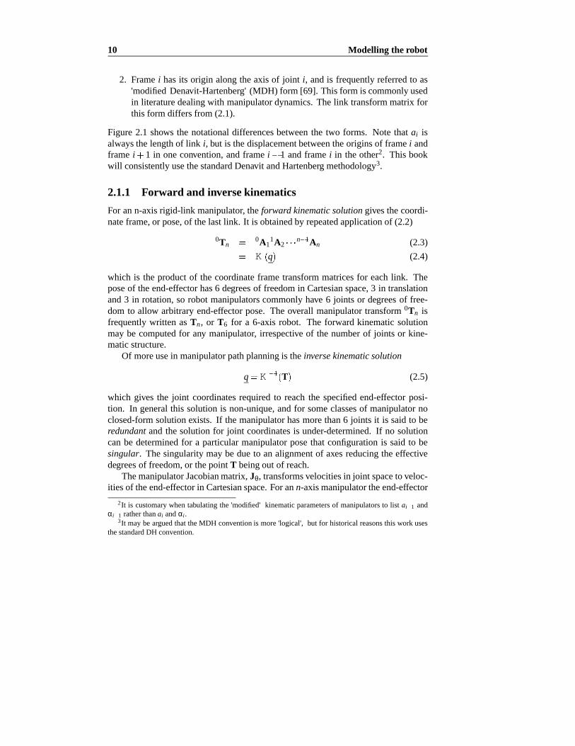
2. Framei hasits origin alongtheaxisof joint i, andis frequentlyreferredto as'modifiedDenavit-Hartenberg' (MDH) form [69]. Thisform is commonlyusedin literaturedealingwith manipulatordynamics.Thelink transformmatrix forthis form differsfrom (2.1).
Figure2.1 shows the notationaldifferencesbetweenthe two forms. Note that ai isalwaysthelengthof link i, but is thedisplacementbetweentheoriginsof framei andframe i 1 in oneconvention,andframei 1 andframe i in theother2. This bookwill consistentlyusethestandardDenavit andHartenberg methodology3.
2.1.1 Forward and inversekinematics
For ann-axisrigid-link manipulator, the forward kinematicsolutiongivesthecoordi-nateframe,or pose,of thelastlink. It is obtainedby repeatedapplicationof (2.2)
0Tn0A1
1A2n 1An (2.3)
K q (2.4)
which is the productof the coordinateframetransformmatricesfor eachlink. Theposeof theend-effectorhas6 degreesof freedomin Cartesianspace,3 in translationand3 in rotation,so robot manipulatorscommonlyhave 6 joints or degreesof free-dom to allow arbitraryend-effector pose. The overall manipulatortransform0Tn isfrequentlywritten asTn, or T6 for a 6-axis robot. The forward kinematicsolutionmay be computedfor any manipulator, irrespective of the numberof joints or kine-maticstructure.
Of moreusein manipulatorpathplanningis the inversekinematicsolution
q K 1 T (2.5)
which gives the joint coordinatesrequiredto reachthe specifiedend-effector posi-tion. In generalthis solutionis non-unique,andfor someclassesof manipulatornoclosed-formsolutionexists. If themanipulatorhasmorethan6 joints it is saidto beredundantandthesolutionfor joint coordinatesis under-determined.If no solutioncanbe determinedfor a particularmanipulatorposethat configurationis saidto besingular. Thesingularitymaybedueto analignmentof axesreducingtheeffectivedegreesof freedom,or thepointT beingout of reach.
ThemanipulatorJacobianmatrix,Jθ, transformsvelocitiesin joint spaceto veloc-itiesof theend-effectorin Cartesianspace.For ann-axismanipulatortheend-effector
2It is customarywhentabulating the 'modified' kinematicparametersof manipulatorsto list ai 1 andα i 1 ratherthanai andα i .
3It maybearguedthat theMDH conventionis more'logical', but for historicalreasonsthis work usesthestandardDH convention.

2.1Manipulator kinematics 11
Cartesianvelocity is
0xn0Jθq (2.6)
tnxntnJθq (2.7)
in baseor end-effectorcoordinatesrespectively andwherex is theCartesianvelocityrepresentedby a 6-vector[199]. For a 6-axismanipulatortheJacobianis squareandprovided it is not singularcan be invertedto solve for joint ratesin termsof end-effectorCartesianrates.TheJacobianwill notbeinvertibleatakinematicsingularity,andin practicewill bepoorly conditionedin thevicinity of thesingularity, resultingin high joint rates.A controlschemebasedonCartesianratecontrol
q 0J 1θ
0xn (2.8)
wasproposedby Whitney [277] andis known as resolvedrate motioncontrol. Fortwo framesA andB relatedby ATB n o a p theCartesianvelocity in frameA maybetransformedto frameB by
Bx BJAAx (2.9)
wheretheJacobianis givenby Paul [200] as
BJA f ATBn o a T p n p o p a T
0 n o a T (2.10)
2.1.2 Accuracy and repeatability
In industrialmanipulatorsthe positionof the tool tip is inferredfrom the measuredjoint coordinatesandassumedkinematicstructureof therobot
T6 K qmeas
Errorswill beintroducedif theassumedkinematicstructurediffersfromthatof theac-tualmanipulator, thatis, K K . Sucherrorsmaybedueto manufacturingtolerancesin link lengthor link deformationdueto load.Assumptionsarealsofrequentlymadeaboutparallelor orthogonalaxes, that is link twist anglesareexactly 0 or exactly
90 , sincethis simplifiesthe link transformmatrix (2.1) by introducingelementsthatareeither0 or 1. In reality, dueto tolerancesin manufacture,theseassumptionarenot valid andleadto reducedrobotaccuracy.
Accuracy refersto the error betweenthe measuredandcommandedposeof therobot. For a robotto move to a commandedposition,theinversekinematicsmustbesolvedfor therequiredjoint coordinates
q6 K 1 T

12 Modelling the robot
Joint α ai di θmin θmax
1 90 0 0 -180 1802 0 431.8 0 -170 1653 -90 20.3 125.4 -160 1504 90 0 431.8 -180 1805 -90 0 0 -10 1006 0 0 56.25 -180 180
Table2.1: Kinematicparametersandjoint limits for thePuma560.All anglesindegrees,lengthsin mm.
While theservo systemmaymove very accuratelyto thecomputedjoint coordinates,discrepanciesbetweenthekinematicmodelassumedby thecontrollerandtheactualrobotcancausesignificantpositioningerrorsat thetool tip. Accuracy typically variesover the workspaceandmay be improved by calibrationprocedureswhich seektoidentify thekinematicparametersfor theparticularrobot.
Repeatabilityrefersto theerrorwith which a robotreturnsto a previously taughtor commandedpoint. In generalrepeatabilityis betterthanaccuracy, andis relatedtojoint servo performance.However to exploit this capabilitypointsmustbemanuallytaughtby 'jogging' the robot, which is time-consumingand takesthe robot out ofproduction.
The AdeptOnemanipulatorfor examplehasa quotedrepeatabilityof 15µm butanaccuracy of 76µm. Thecomparatively low accuracy anddifficulty in exploiting re-peatabilityaretwo of thejustificationsfor visualservoingdiscussedearlierin Section1.1.
2.1.3 Manipulator kinematic parameters
As alreadydiscussedthe kinematicparametersof a robot are importantin comput-ing the forwardandinversekinematicsof the manipulator. Unfortunately, asshownin Figure2.1, therearetwo conventionsfor describingmanipulatorkinematics.Thisbookwill consistentlyusethestandardDenavit andHartenberg methodology, andtheparticularframeassignmentsfor the Puma560areasperPaul andZhang[202]. Aschematicof therobotandtheaxisconventionsusedis shown in Figure2.2. For zerojoint coordinatesthearmis in a right-handedconfiguration,with theupperarmhori-zontalalongtheX-axisandthelowerarmvertical.Theuprightor READY position4 isdefinedby q 0 90 90 0 0 0 . OtherssuchasLee[166] considerthezero-angleposeasbeingleft-handed.
4TheUnimationVAL languagedefinesthesocalled'READY position' wherethearmis fully extendedandupright.

2.1Manipulator kinematics 13
Figure2.2: Detailsof coordinateframesusedfor thePuma560shown herein itszeroanglepose(drawing by LesEwbank).
Thenon-zerolink offsetsandlengthsfor thePuma560,which maybemeasureddirectly, are:
distancebetweenshoulderandelbow axesalongtheupperarmlink, a2;
distancefrom the elbow axis to the centerof sphericalwrist joint; along thelowerarm,d4;
offsetbetweentheaxesof joint 4 andtheelbow, a3;

14 Modelling the robot
offsetbetweenthewaistandjoint 4 axes,d3.
The kinematicconstantsfor thePuma560aregivenin Table2.1. Theseparam-etersarea consensus[60,61] derived from several sources[20,166,202,204,246].Thereis somevariationin the link lengthsandoffsetsreportedby variousauthors.Comparisonof reportsis complicatedby the varietyof differentcoordinatesystemsused.Somevariationsin parameterscouldconceivablyreflectchangesto thedesignormanufactureof therobotwith time,while othersaretakento beerrors.Leealonegivesa valuefor d6 which is thedistancefrom wrist centerto thesurfaceof themountingflange.
Thekinematicparametersof arobotareimportantnotonly for forwardandinversekinematicsasalreadydiscussed,but arealsorequiredin thecalculationof manipula-tor dynamicsas discussedin the next section. The kinematicparametersenterthedynamicequationsof motionvia thelink transformationmatricesof (2.1).
2.2 Manipulator rigid-body dynamics
Manipulatordynamicsis concernedwith the equationsof motion, theway in whichthe manipulatormoves in responseto torquesappliedby the actuators,or externalforces.Thehistoryandmathematicsof thedynamicsof serial-linkmanipulatorsarewell coveredby Paul [199] andHollerbach[119]. Therearetwo problemsrelatedtomanipulatordynamicsthatareimportantto solve:
inversedynamicsin which themanipulator'sequationsof motionaresolvedforgivenmotion to determinethegeneralizedforces,discussedfurther in Section2.5,and
directdynamicsin whichtheequationsof motionareintegratedtodeterminethegeneralizedcoordinateresponseto appliedgeneralizedforcesdiscussedfurtherin Section2.2.3.
Theequationsof motionfor ann-axismanipulatoraregivenby
Q M q q C q q q F q G q (2.11)
where
q is thevectorof generalizedjoint coordinatesdescribingtheposeof themanipulator
q is thevectorof joint velocities;q is thevectorof joint accelerations
M is thesymmetricjoint-spaceinertiamatrix,or manipulatorinertiatensor

2.2Manipulator rigid-body dynamics 15
C describesCoriolisandcentripetaleffects— Centripetaltorquesarepro-portionalto q2
i , while theCoriolis torquesareproportionalto qi q j
F describesviscousandCoulombfriction andis notgenerallyconsideredpartof therigid-bodydynamics
G is thegravity loadingQ is thevectorof generalizedforcesassociatedwith thegeneralizedcoor-
dinatesq.
Theequationsmaybederivedvia a numberof techniques,includingLagrangian(energy based),Newton-Euler, d'Alembert [96,167] or Kane's [143] method. Theearliestreportedwork was by Uicker [254] and Kahn [140] using the Lagrangianapproach.Due to the enormouscomputationalcost,O n4 , of this approachit wasnot possibleto computemanipulatortorquefor real-timecontrol. To achieve real-timeperformancemany approachesweresuggested,includingtablelookup[209] andapproximation[29,203].Themostcommonapproximationwasto ignorethevelocity-dependentterm C, sinceaccuratepositioningandhigh speedmotion areexclusivein typical robot applications. Othershave usedthe fact that the coefficientsof thedynamicequationsdonot changerapidly sincethey area functionof joint angle,andthusmaybe computedat a fractionof the rateat which the equationsareevaluated[149,201,228].
Orin etal. [195]proposedanalternativeapproachbasedontheNewton-Euler(NE)equationsof rigid-bodymotionappliedto eachlink. Armstrong[23] thenshowedhowrecursionmight beappliedresultingin O n complexity. Luh et al. [177] providedarecursiveformulationof theNewton-Eulerequationswith linearandangularvelocitiesreferredto link coordinateframes.They suggesteda time improvementfrom 7 9sfortheLagrangianformulationto 4 5ms, andthusit becamepracticalto implement'on-line'. Hollerbach[120] showed how recursioncould be appliedto the Lagrangianform, andreducedthecomputationto within a factorof 3 of therecursive NE. Silver[234] showed theequivalenceof therecursive LagrangianandNewton-Eulerforms,andthatthedifferencein efficiency is dueto therepresentationof angularvelocity.
“Kane's equations”[143] provideanothermethodologyfor deriving theequationsof motionfor aspecificmanipulator. A numberof 'Z' variablesareintroducedwhich,whilenotnecessarilyof physicalsignificance,leadtoadynamicsformulationwith lowcomputationalburden. Wampler[267] discussesthe computationalcostsof Kane'smethodin somedetail.
The NE andLagrangeforms can be written generallyin termsof the Denavit-Hartenberg parameters— howeverthespecificformulations,suchasKane's,canhavelower computationalcost for the specificmanipulator. Whilst the recursive formsarecomputationallymoreefficient, the non-recursive forms computethe individualdynamicterms(M , C andG) directly.

16 Modelling the robot
Method Multiplications Additions For N=6Mul Add
Lagrangian[120] 3212n4 86 5
12n3 25n4 6613n3 66,271 51,548
17114n2 531
3n 12912n2 421
3n128 96
RecursiveNE [120]
150n 48 131n 48 852 738
Kane[143] 646 394SimplifiedRNE[189]
224 174
Table2.2: Comparisonof computationalcostsfor inversedynamicsfrom varioussources.Thelastentryis achievedby symbolicsimplificationusingthesoftwarepackageARM.
A comparisonof computationcostsis givenin Table2.2. Thereareconsiderablediscrepanciesbetweensources[96,120,143,166,265] on thecomputationalburdensof thesedifferentapproaches.Conceivablesourcesof discrepancy includewhetheror not computationof link transformmatricesis included,andwhetherthe result isgeneral,or specificto a particularmanipulator.
2.2.1 RecursiveNewton-Euler formulation
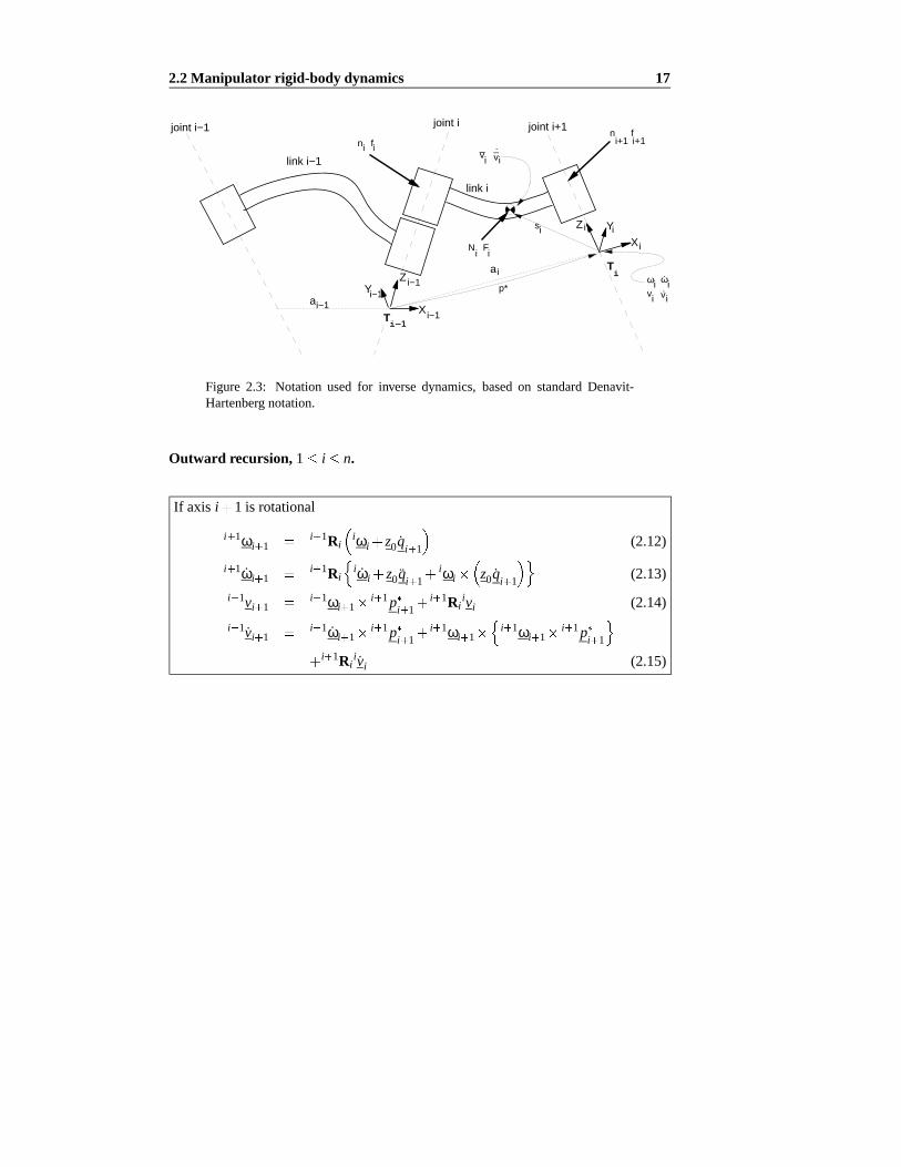
Therecursive Newton-Euler(RNE) formulation[177] computesthe inversemanipu-lator dynamics,that is, thejoint torquesrequiredfor a givensetof joint coordinates,velocitiesandaccelerations.The forward recursionpropagateskinematicinforma-tion — suchasangularvelocities,angularaccelerations,linearaccelerations— fromthebasereferenceframe(inertial frame)to theend-effector. Thebackwardrecursionpropagatesthe forcesandmomentsexertedon eachlink from theend-effectorof themanipulatorto thebasereferenceframe5. Figure2.3shows thevariablesinvolvedinthecomputationfor onelink.
Thenotationof Hollerbach[120] andWalkerandOrin [265] will beusedin whichthe left superscriptindicatesthe referencecoordinateframe for the variable. Thenotationof Luh etal. [177] andlaterLee[96,166] is considerablylessclear.
5It shouldbenotedthatusingMDH notationwith its differentaxisassignmentconventionstheNewtonEulerformulationis expresseddifferently[69].
2.2Manipulator rigid-body dynamics 17
joint i−1 joint i joint i+1
link i−1
link i
Ti−1
Tiai
Xi
YiZi
ai−1
Zi−1
Xi−1
Yi−1p* vi
.vi
.ωiωi
n fi i
N Fi i
vi
.vi
_ _i+1 i+1
n f
si
Figure 2.3: Notation usedfor inversedynamics,basedon standardDenavit-Hartenberg notation.
Outward recursion,1 i n.
If axis i 1 is rotational
i 1ωi 1i 1Ri
iωi z0qi 1
(2.12)
i 1ωi 1i 1Ri
iωi z0qi 1
iωi z0qi 1
(2.13)
i 1vi 1i 1ωi 1
i 1pi 1
i 1Riivi (2.14)
i 1vi 1i 1ωi 1
i 1pi 1
i 1ωi 1i 1ωi 1
i 1pi 1
i 1Rii vi (2.15)

18 Modelling the robot
If axis i 1 is translational
i 1ωi 1i 1Ri
iωi (2.16)i 1ωi 1
i 1Riiωi (2.17)
i 1vi 1i 1Ri z0q
i 1ivi
i 1ωi 1i 1p
i 1(2.18)
i 1vi 1i 1Ri z0q
i 1i vi
i 1ωi 1i 1p
i 1
2 i 1ωi 1i 1Ri z0q
i 1
i 1ωi 1i 1ωi 1
i 1pi 1
(2.19)
i viiωi si
iωiiωi si
i vi (2.20)iFi mi
i vi (2.21)iNi Ji
iωiiωi Ji
iωi (2.22)
Inward recursion,n i 1.
i fi
iRi 1i 1 f
i 1iF i (2.23)
iniiRi 1
i 1ni 1i 1Ri
i pi
i 1 fi 1
i pi
siiFi
iNi (2.24)
Qi
iniT iRi 1z0 if link i 1 is rotational
i fi
TiRi 1z0 if link i 1 is translational
(2.25)
where
i is thelink index, in therange1 to nJi is themomentof inertiaof link i aboutits COMsi is thepositionvectorof theCOM of link i with respectto framei
ωi is theangularvelocity of link iωi is theangularaccelerationof link ivi is thelinearvelocity of frameivi is thelinearaccelerationof frameivi is thelinearvelocity of theCOM of link ivi is thelinearaccelerationof theCOM of link ini is themomentexertedon link i by link i 1

2.2Manipulator rigid-body dynamics 19
fi
is theforceexertedonlink i by link i 1Ni is thetotalmomentat theCOM of link iFi is thetotal forceat theCOM of link iQ
iis theforceor torqueexertedby theactuatorat joint i
i 1Ri is theorthonormalrotationmatrix definingframei orientationwith re-spectto framei 1. It is theupper3 3 portionof thelink transformmatrixgivenin (2.1).
i 1Ri
cosθi cosαi sinθi sinαi sinθi
sinθi cosαi cosθi sinαi cosθi
0 sinαi cosαi
(2.26)
iRi 1i 1Ri
1 i 1RiT (2.27)
i pi
is thedisplacementfromtheorigin of framei 1 to framei with respectto framei.
i pi
ai
di sinαi
di cosαi
(2.28)
It is thenegative translationalpartof i 1A i1.
z0 is a unit vectorin Z direction,z0 0 0 1
Note that the COM linear velocity givenby equation(2.14)or (2.18)doesnot needto becomputedsinceno otherexpressiondependsuponit. Boundaryconditionsareusedto introducetheeffectof gravity by settingtheaccelerationof thebaselink
v0 g (2.29)
whereg is thegravity vectorin thereferencecoordinateframe,generallyactingin thenegative Z direction,downward.Basevelocity is generallyzero
v0 0 (2.30)
ω0 0 (2.31)
ω0 0 (2.32)
2.2.2 Symbolicmanipulation
TheRNE algorithmis straightforwardto programandefficient to executein thegen-eralcase,but considerablesavingscanbemadefor thespecificmanipulatorcase.Thegeneralform inevitably involvesmany additionswith zeroandmultiplicationswith 0,

20 Modelling the robot
1 or -1, in the variousmatrix andvectoroperations.The zerosandonesareduetothe trigonometricterms6 in the orthonormallink transformmatrices(2.1) aswell aszero-valuedkinematicandinertial parameters.Symbolicsimplificationgatherscom-monfactorsandeliminatesoperationswith zero,reducingtherun-timecomputationalload,at theexpenseof a once-onlyoff-line symboliccomputation.Symbolicmanip-ulation can alsobe usedto gain insight into the effects andmagnitudesof variouscomponentsof theequationsof motion.
Early work in symbolicmanipulationfor manipulatorswasperformedwith spe-cial toolsgenerallywritten in Fortranor LISP suchasARM [189], DYMIR [46] andEMDEG [40]. Laterdevelopmentof generalpurposecomputeralgebratoolssuchasMacsyma,REDUCEandMAPLE hasmadethiscapabilitymorewidely available.
In thiswork a generalpurposesymbolicalgebrapackage,MAPLE [47], hasbeenusedto computethe torqueexpressionsin symbolicform via a straightforwardim-plementationof the RNE algorithm. Comparedto symboliccomputationusing theLagrangianapproach,computationof the torqueexpressionsis very efficient. Theseexpressionsarein sumof productform, andcanbeextremelylong. For exampletheexpressionfor thetorqueon thefirst axisof a Puma560is
τ1 C23Iyz3q2
sx12m1q1
S23Iyz3q23
Iyy2C22q1
C2 Iyz2q2
andcontinuesonfor over16,000terms.Suchexpressionsareof little valuefor on-linecontrol,but areappropriatefor furthersymbolicmanipulationto analyzeandinterpretthesignificanceof variousterms.For examplethesymbolicelementsof theM , C andG termscanbereadilyextractedfrom thesumof productform, overcomingwhat isfrequentlycitedasanadvantageof theLagrangianformulation— thattheindividualtermsarecomputeddirectly.
Evaluatingsymbolicexpressionsin this simple-mindedway resultsin a lossofthefactorizationinherentin theRNEprocedure.However with appropriatefactoriza-tion duringsymbolicexpansion,a computationallyefficient form for run-timetorquecomputationcanbegenerated,seeSection2.6.2. MAPLE canthenproducethe 'C'languagecodecorrespondingto the torqueexpressions,for example,automaticallygeneratingcodefor computed-torquecontrol of a specificmanipulator. MAPLE isalsocapableof generatingLATEX styleequationsfor inclusionin documents.
6Commonmanipulatorshave link twists of 0 , 90 or 90 leadingto zero or unity trigonometricresults.

2.2Manipulator rigid-body dynamics 21
As discussedpreviously, thedynamicequationsareextremelycomplex, andthusdifficult to verify, but anumberof checkshavebeenmade.Theequationsof motionofa simpletwo-link examplein Fuet al. [96] wascomputedandagreedwith theresultsgiven. For thePuma560this is prohibitive,but somesimplecheckscanstill beper-formed.Thegravity termis readilyextractedandis simpleenoughto verify manually.The manipulatorinertia matrix is positive definiteandits symmetrycanbe verifiedsymbolically. A colleague[213] independentlyimplementedthedynamicequationsin MAPLE, usingthe Lagrangianapproach.MAPLE wasthenusedto computethedifferencebetweenthetwo setsof torqueexpressions,which aftersimplificationwasfoundto bezero.
2.2.3 Forward dynamics
Equation(2.11)maybeusedto computethe so-calledinversedynamics,that is, ac-tuatortorqueasa functionof manipulatorstateandis usefulfor on-linecontrol. Forsimulationthedirect,integralor forward dynamicformulationis requiredgiving jointmotionin termsof input torques.
Walker andOrin [265] describeseveral methodsfor computingthe forward dy-namics,andall makeuseof anexisting inversedynamicssolution. Using the RNEalgorithmfor inversedynamics,thecomputationalcomplexity of theforwarddynam-ics using 'Method 1' is O n3 for an n-axis manipulator. Their other methodsareincreasinglymoresophisticatedbut reducethecomputationalcost,thoughstill O n3 .Featherstone[89] hasdescribedthe'articulated-bodymethod' for O n computationof forward dynamics,however for n 9 it is moreexpensive thanthe approachofWalkerandOrin. AnotherO n approachfor forwarddynamicshasbeendescribedby Lathrop[160].
2.2.4 Rigid-body inertial parameters
Accuratemodel-baseddynamiccontrol of a manipulatorrequiresknowledgeof therigid-bodyinertialparameters.Eachlink hastenindependentinertialparameters:
link mass,mi;
threefirst moments,which may be expressedas the COM location, si, withrespectto somedatumon thelink or asamomentSi misi ;
six secondmoments,which representtheinertiaof thelink abouta givenaxis,typically throughtheCOM. Thesecondmomentsmaybeexpressedin matrixor tensorform as
JJxx Jxy Jxz
Jxy Jyy Jyz
Jxz Jyz Jzz
(2.33)

22 Modelling the robot
Parameter Value
m1 13.0m2 17.4m3 4.80m4 0.82m5 0.35m6 0.09
Table2.3: Link massdata(kg).
wherethediagonalelementsarethemomentsof inertia, andtheoff-diagonalsareproductsof inertia. Only six of thesenineelementsareunique: threemo-mentsandthreeproductsof inertia.
For any pointin arigid-bodythereis onesetof axesknownastheprincipal axesof inertia for which the off-diagonalterms,or products,arezero. Theseaxesaregivenby theeigenvectorsof theinertiamatrix(2.33)andtheeigenvaluesaretheprincipalmomentsof inertia.Frequentlytheproductsof inertiaof therobotlinks arezerodueto symmetry.
A 6-axismanipulatorrigid-bodydynamicmodelthusentails60 inertial parame-ters. Theremay be additionalparametersper joint dueto friction andmotor arma-ture inertia. Clearly, establishingnumericvaluesfor this numberof parametersisa difficult task. Many parameterscannotbemeasuredwithout dismantlingtherobotandperformingcarefulexperiments,thoughthis approachwasusedby Armstrongetal. [20]. Most parameterscouldbederivedfrom CAD modelsof therobots,but thisinformationis oftenconsideredproprietaryandnotmadeavailableto researchers.Therobotusedin this work, thePuma560,wasdesignedin thelate1970'sandprobablypredateswidespreadCAD usage.Thereis alsoaconsiderableliteratureregardingesti-mationof inertialparametersfrom onlinemeasurementof manipulatorstateandjointtorques[130].
Tarn andBejczy [245,247], Armstrong[22] andLeahy[161,165,257] have allreportedsuccessfulmodel-basedcontrolof thePuma560,yet thereis significantdif-ferencein theparametersetsused.Thismayin factindicatethattherigid-bodyeffectsdo not dominatethedynamicsof this robot,or that“somefeedforwardis betterthanno feedforward”. This issuewill be revisited in Section2.4. Comparisonsof thepublishedmodeldataarecomplicatedby the differentcoordinateframes,kinematicconventionsandmeasurementunits usedin the original reports. The first stepis toconvert all reporteddatato a commonsetof unitsandcoordinateframes,andthesedataare reportedandcomparedin [60,61]. Somedatasetsare to be preferredtoothersdueto the methodologiesusedto obtainthem. The remainderof this sectioncomprisesanabbreviatedreportof thatcomparisonwork andtabulatesthepreferred

2.2Manipulator rigid-body dynamics 23
Parameter Value
sx1 -sy1 -sz1 -sx2 -363.8sy2 6sz2 77.4sx3 0sy3 -14sz3 70sx4 0sy4 -19sz4 0sx5 0sy5 0sz5 0sx6 0sy6 0sz6 32
Table2.4: Link COM positionwith respectto link frame(mm).
inertialparametervalues.Link massdatafor joints 2-6 givenin Table2.3 arebasedon theresultsof Arm-
strongetal. [20] whoactuallydisassembledtherobotandweighedthelinks. Theoftencited dataof Tarnet al. [246] is basedon estimatedmassfrom models,dimensionaldataandassumedmassdistributionanddensities,which is likely to belessaccurate.A similar approachappearsto have beentakenby Paul et al. [204]. Armstronghow-ever doesnot give a valuefor m1, soTarn's valueis presentedin the table. It canbeshown however that theparameterm1 doesnot appearin theequationsof motion—it is nota baseparameter[148,153].
Link centerof gravity datagivenin Table2.4 is againbasedon Armstronget al.who measuredtheCOM of thedisassembledlinks ona knife-edge.Tarnet al.'s datais againanestimatebasedonmodelsof thearmstructure.
It is difficult to meaningfullycomparethesedatasets,andcontrastthemwith thosefor therobotusedin thiswork. Theapproachproposedhereis to comparethegravityloadingtermsfor joints 2 and3 — thoselinks for which gravity load is significant.A smallnumberof gravity loadcoefficientsencapsulatea largernumberof massandCOM parameters.Thegravity loadingsarereadilygeneratedfromthesymbolictorque

24 Modelling the robot
Parameter Armstrong Tarn RCCL
g1 -0.896 -0.977 -0.928(CP30/g)g2 0.116 0.235 0.0254(CP21/g)g3 0 -0.00980g4 0 0g5 -2.88e-3 0.34e-3 -2.88e-3(CP50/g)g6 0 0g7 -0.104 -0.112 0.104(CP22/g)g8 3.80 5.32 -3.79(CP20/g)
Table2.5: Comparisonof gravity coefficients(N.m) from severalsources.
equationsestablishedearlier, andaregivenby
τg3
gm6 m5 m4 D4 sz3m3 m4sy4 S23
m3 m4 m5 m6 A3 m3sx3 C23
sz4m4 sy5m5 sy6m6C6 C23S4
S23S5sy6m6S6
sz6m6 sz5m5 C23S5C4 S23C5
S6sy6m6C23C4C5τg2
gm2sx2 m2 m3 m4 m5 m6 A2 C2
sy2m2S2τg3
g(2.34)
whereAi andDi arekinematicconstants,Ci cosθi andSi sinθi. Thesemaybewritten moresuccinctlyin termsof a numberof coefficientswhich arefunctionsoflink mass,centerof gravity andsomekinematiclengthparameters;
τg3
gg1S23 g2C23 g3C23S4 g4S23S5S6
g5 S5C4C23 S23C5 g6C5C4C23S6 (2.35)τg2
gg7S2 g8C2
τg3
g(2.36)
Thesecoefficientsareevaluatedandcomparedin Table2.5alongwith thoseusedby the RCCL robot control package[115,175]. Thereis closeagreementbetweenthemagnitudesof thecoefficientsfrom Armstrongandthoseusedin RCCL.Dif ferentkinematicconventionsusedby RCCL, or the sign of the gearratios, may explainthe differencein sign for the joint 2 coefficientsg7 andg8. The RCCL valueswere

2.2Manipulator rigid-body dynamics 25
0 0.5 1 1.5 2 2.5 3-80
-60
-40
-20
0
20
40
60
80
q2 (radl)
tau_
g2 (
Nm
@lo
ad)
Figure2.4: Measuredandestimatedgravity load on joint 2, τg2 θ2 , for θ3π 2. Torquemeasurements(shown dotted)arederived from measuredmotor
currentandcorrectedto eliminatetheeffect of Coulombfriction. Also shown istheestimatedgravity loadbasedonmaximumlikelihoodfit (dotdash),parametervaluesof Armstrong(solid)andTarn(dashed).
determinedusinganexperimentalproceduresimilar to thatdescribedby Lloyd [175]for a Puma2607.
Figure2.4shows thejoint 2 torquedueto gravity, versuschangingshoulderjointangle. Theshoulderjoint wasmoved forwardandbackwardover the angularrangeat very low speedto eliminateany torquecomponentdueto viscousfriction. Jointtorqueis derivedfrom measuredmotorcurrentusingmotortorqueconstantsfrom Ta-ble 2.14. TheCoulombfriction effect is very pronounced,andintroducessignificanthysteresisin the torqueversusangleplot. The torquein Figure 2.4 hasbeencor-rectedfor Coulombfriction usingthe identifiedfriction parametersfrom Table2.12,but somehysteresisremainsat q2 π. It is speculatedthat this is dueto position-dependentCoulombfriction effectsoutsidethe rangeof joint anglesover which thefriction estimationexperimentswereconducted.
A maximumlikelihood fit to theexperimentaldatais alsoshown in thefigure. Itcanbe seenthat the estimatedtorqueusingArmstrong's datais slightly lower than
7JohnLloyd, privatecommunication.

26 Modelling the robot
Parameter β (N.m) φ (rad)
Armstrong 46.1 2.6e-3Tarn 61.8 19.5e-3Max.Likelihood 52.9 -10.8e-3
Table2.6: Comparisonof shouldergravity loadmodelsin cosineform.
Parameter Value
Jxx1 -Jyy1
0.35†Jzz1 -Jxx2 0.130Jyy2
0.524Jzz2 0.539Jxx3 0.066Jyy3
0.0125Jzz3 0.086Jxx4 1.8e-3Jyy4
1.8e-3Jzz4 1.3e-3Jxx5 0.30e-3Jyy5
0.30e-3Jzz5 0.40e-3Jxx6 0.15e-3Jyy6
0.15e-3Jzz6 0.04e-3
Table2.7: Link inertiaabouttheCOM (kg m2). -Thisvalue,dueto Armstrong,is in fact theinertiaaboutthelink frameJyy1 m1 s2
x1s2z1
notabouttheCOM.
thatmeasured,while thatbasedon Tarn's datais somewhathigher. Thegravity loadmaybewritten in theform
τg2 βcos θ2 φ (2.37)
whereβ is the magnitudeandφ the phase. The coefficients for the variousformsarecomparedin Table2.6, andin termsof magnitudethemaximumlikelihood fit isbracketedby themodelsof TarnandArmstrong,asis alsoevident from Figure2.4.Despitethepreviousobjectionsto themethodologyof Tarnetal. their datagivesa fitfor thegravity loadof joint 2 thatis asgoodasthatof Armstrong.
Link inertiaaboutthecenterof gravity is givenin Table2.7,basedlargelyonArm-strong.Armstrong'sdatafor links1 to 3 wasdeterminedexperimentally, while thatfor

2.2Manipulator rigid-body dynamics 27
thewrist links wasestimated.HoweverArmstrong'svalueof Jyy18 is in facttheinertia
measuredaboutthelink frame,Jyy1Jyy1 m1 s2
x1s2z1
, not theCOM asindicatedin [20], sincethetwo inertialcomponentscannotbeseparatedby measurementsat thelink9.
2.2.5 Transmissionand gearing
For aG:1 reductiondrive thetorqueat thelink is G timesthetorqueatthemotor. Theinertiaof themotorat thelink is amplifiedby G2, asis theviscousfriction coefficient.For rotary joints the quantitiesmeasuredat the link, subscriptl , are relatedto themotorreferencedquantities,subscriptm, asshown in Table2.8.Themanipulatorgearratios10 givenin Table2.9arederivedfrom severalsources[20,190,262].
Thedesignof therobot'swrist is suchthatthereis considerablecouplingbetweentheaxes,thatis, rotationof onemotorresultsin therotationof severalwrist links. Therelationshipbetweenlink andmotoranglesis clearlyexpressedin matrix form
θm Gθl θl G 1θm (2.38)
where
G
G1 0 0 0 0 00 G2 0 0 0 00 0 G3 0 0 00 0 0 G4 0 00 0 0 G45G5 G5 00 0 0 G46G6 G56G6 G6
(2.39)
G 1
1G1
0 0 0 0 00 1
G20 0 0 0
0 0 1G3
0 0 00 0 0 1
G40 0
0 0 0 G45G4
1G5
0
0 0 0 G46 G56G45G4
G56G5
1G6
(2.40)
Thecross-couplingratioshave beendeterminedfrom examinationof theengineeringdrawingsandcorrespondwith thenumericalvaluesgivenby [262]. Thesehave alsobeenverifiedexperimentally.
8Jzz1 in thesourcepaper, dueto differentcoordinateconventionsused.9B. Armstrong,privatecommunication.
10The sign of the ratio is due to the conventionfor directionof rotationof the motor (definedby thedigital position-loopencodercounter, seeSection2.3.6),andthe conventionfor directionof link rotationwhich is definedby thekinematicmodel.Negativemotorcurrentresultsin positivemotortorque.

28 Modelling the robot
Jl G2Jm
Bl G2Bm
τCl GτCm
τl Gτm
θl θm Gθl θm G
Table2.8: Relationshipbetweenloadandmotorreferencedquantitiesfor gearratioG.
Joint Gearratio
G1 -62.6111G2 107.815G3 -53.7063G4 76.03636G5 71.923G6 76.686G45 1 G5G46 1 G6
G56 13 72
Table2.9: Puma560gearratios.
2.2.6 Quantifying rigid body effects
Thenumericvaluesof theinertialparametersobtainedabove maybesubstitutedintothe equationsof motion. With somemanipulationthis allows the variousdynamiceffectsto bequantifiedandtheboundsdueto changein configurationestablished.ForinstanceFigures2.5,2.6and2.7show respectively theinertiaat joint 1 and2 andthegravity loadat joint 2, all plottedasfunctionsof manipulatorconfiguration.
Therearetwocomponentsof inertia'seen'by themotor. Oneis dueto therotatingarmature,andtheotherdueto the rigid-bodydynamicsof the link reflectedthroughthegearsystem.Thetotalinertiasetstheupperboundonacceleration,andalsoaffectsthedynamicsof theaxiscontrol loop. It is insightful to plot total inertianormalizedwith respectto the armatureinertia,Jm, sincethis clearlyshowstheinertiacomparedwith theunloaded(η 1) case.Thenormalizedinertiais definedto be
ηii q 1M ii q
G2i Jmi
(2.41)
whereM is themanipulatorinertiamatrix from (2.11),andJmi andGi arethemotorarmatureinertiaandthereductiongearratio respectively for joint i. Thenormalized

2.2Manipulator rigid-body dynamics 29
0
6
5
4
3
2
1
0
q30
32
10
-1-2
-3
q20
32 1 0 -1 -2
-3
η11
η12
Figure2.5: Plot of normalizedinertia for joint 1 asa function of shoulderandelbow configuration. Shown is the diagonalterm η11 andthe inertial couplingtermη12. Anglesin rads.
q30 3210-1-2-3
0
2
1.5
1
0.5
0
η22
η23
η21
Figure2.6: Plotof normalizedinertiafor joint 2 asa functionof elbow configura-tion. Shown is thediagonaltermη22 andtheinertialcouplingtermsη21 andη23.Anglesin rads.

30 Modelling the robot
0
40
20
0
-20
-40
q30
32
10
-1-2
-3
q20
32 1 0 -1 -2
-3
Figure2.7: Gravity load (N.m) on joint 2, τg2 q2 q3 . Anglesin rads. Gravityloadvariesbetween 46N m or 48% of thefuselimited torque.
inertial couplingis definedto be
ηi j qM i j q
G2i Jmi
(2.42)
Thenormalizeddiagonalandoff-diagonalinertiaelementsfor Pumajoints1 and2 areshown in Figures2.5 and2.6 asa functionof configuration.Theoff-diagonaltermsarerelatively small in magnitudecomparedto the diagonalvalues. The rigid-bodydynamicequationsfrom Section2.2canbeusedto computetheminimaandmaximaof thenormalizedinertias,andthesearesummarizedin Table2.10. Thevariationismostpronouncedfor thewaistandshoulderjoints. Gravity load,plottedin Figure2.7for joint 2, showsthatgravity torqueis significantcomparedto thetorquelimit of theactuator. The relative significanceof variousdynamictermsis examinedfurther inSection2.4.
2.2.7 Robot payload
The inertia of the load, in this work a camera,hasbeencomputedfrom massanddimensionaldataassuminguniformmassdistributionwithin eachof thecamerabodyandlens.Theresultsaretabulatedin Table2.11.Thecamerainertiawhenreferredto

2.3Electro-mechanicaldynamics 31
Quantity Minimum Maximum Max/Min
η11 2.91 6.35 2.2η12 -0.75 0.75 -η22 2.57 3.24 1.3η33 1.63 -η44 1.01 -η55 1.01 -η66 1.00 -
Table2.10: Minimum andmaximumvaluesof normalizedinertia,basedon pre-ferredarmatureinertiadatafrom Table2.13.
Component Value
mlens 0 270kgmcam 0 155kgIzz 1 0 10 3kg m2
Ixx 6 2 10 3kg m2
I1 0 417kg m2
η5 0 034η6 0 005η1 0 532
Table2.11:Massandinertiaof end-mountedcamera.InertiaIxx andIzz arecom-putedwith respectto thecenterof the robotwrist, seeFigure4.11. I1 is camerainertiawith respectto thejoint 1 axisat maximumarmextension.η i is thenor-malizedcamerainertiawith respectto joint i, thatis, Icam G2
i Jmi .
thewrist motorsandnormalizedis insignificant.However the inertiacontribution tojoint 1 whenthearmis fully extended,I1, is significant.
2.3 Electro-mechanicaldynamics
Thissectionprovidesdetailsaboutthedynamiceffectsdueto therobot'scontrolelec-tronics,actuatorsandmechanicaltransmission.Theseeffectsareat leastassignificantastherigid-bodyeffectsjust reviewedthoughthey arelesswell coveredin thelitera-ture,perhapsdueto therobotspecificnatureof theseeffects.

32 Modelling the robot
rad/s
stiction
low speedregime
τc−
+τc
τ
τs
(Nm)
q.
viscousfriction, B
Coulombfriction
Figure2.8: Typical friction versusspeedcharacteristic.The dashedlinesdepictasimplepiecewise-linearfriction modelcharacterizedby slope(viscousfriction)andintercept(Coulombfriction).
2.3.1 Friction
Dynamiceffectsdueto the transmissionor drive systemaresignificant,particularlyas the drive train becomesmorecomplex. The additionof gearsto amplify motortorqueleadsto increasedviscousfriction andnon-lineareffectssuchasbacklashandCoulombfriction.
For a gearedmanipulator, suchasthePuma,friction is a dominantdynamicchar-acteristic.A typical friction torqueversusspeedcharacteristicis shown in Figure2.8.Thedashedline representsthesimplefriction model
τ f Bθ τc (2.43)
wheresloperepresentsviscousfriction, andoffsetrepresentsCoulombfriction. Thelatteris frequentlymodelledby thenon-linearfunction
τc
0 if q 0τc if q 0τc if q 0
(2.44)
andin general τc τc . Staticfriction, or stiction,is thetorquethatis necessarytobringastationaryjoint into motion,andcanbeconsiderablygreaterthantheCoulomb

2.3Electro-mechanicaldynamics 33
friction value. Themorecomplex model,representedby thesolid line, is significantonly for very low velocities[22]. Thenegative slopecanbeattributedto theStribeckeffect due to mixed lubrication — the load is partially, but increasingly, lifted bylubricant,resultingin decreasingfriction. Thisnegativeslopecharacteristiccanresultin instabilitywith simplePID joint controlschemesat low velocity. Whenthecontactis fully lubricatedviscousfriction is evident.
The friction parametersdiscussedrepresenttotal lumpedfriction due to motorbrushes,bearingsandtransmission.They aredependentuponmany factorsincludingtemperature,stateof lubrication,andto a small extent shaftangle. Armstrong[21,22] providesdetailedinvestigationsof thelow speedandangulardependenceof jointfriction for aPuma560manipulator.
Classictechniquesfor determiningfriction are basedon the simple piecewise-linearfriction modelof (2.43). A joint is movedat constantvelocity andtheaveragetorque(typically determinedfrom motorcurrent)is measured.This is repeatedfor arangeof velocities,bothpositiveandnegative, from which theslope(viscousfrictioncoefficient) andintercepts(Coulombfriction torques)canbedetermined.Measure-mentof joint friction characteristicsusingthisapproachhavebeenpreviouslyreportedfor a Puma260[175] anda Puma560[173].
The friction valuesfor the robot usedin this work have beendeterminedexper-imentallyandaresummarizedin Table2.12. Coulombfriction andviscousfrictionweredeterminedby measuringaveragejoint currentfor variousjoint speedsover ashortangularrangeaboutthevertical'READY' position.Thiswasdoneto eliminatethetorquecomponentdueto gravity whichwouldotherwiseinfluencetheexperiment.A typical plot of currentversusvelocity is shown in Figure2.9. Givenknowledgeofthemotortorqueconstantfrom Table2.14,viscousandCoulombfriction valuesmaybedeterminedfrom theslopeandinterceptrespectively. A robot 'work out' programwasrun prior to themeasurementsbeingtaken,soasto bring joints andlubricantupto ' typical' working temperature.Thereis no evidenceof the negative slopeon thefriction curve at thevelocitiesusedhere.Thelowestvelocity in eachtestwas5 /s atthe link, which is approximately5% and2% of thepeakvelocitiesfor the baseandwrist jointsrespectively.
From Table2.12 it is clear that somefriction parametersshow considerablede-pendenceon the directionof rotation. Statisticalanalysisof the meanandvarianceof the samplepoints[266] for positive andnegative velocity for eachjoint indicatethatat the95%confidencelevel the friction valuesarenot equal,apartfrom viscousfriction valuesfor joints 1 and6. Armstrong[22] showedstatisticallythatCoulombandviscousfriction hadseparatevaluesfor positiveandnegativevelocities.For linearsystemdesignandsimulationthemeanviscousfriction valuewill beused.
Stiction, τs, wasmeasuredby increasingthe joint currentuntil joint motion oc-curred11. For thosejoints subjectto gravity load the robot waspositionedso asto
11Takenasincreasingencodervaluefor 5 consecutivesampleintervals.

34 Modelling the robot
-40 -30 -20 -10 0 10 20 30 40-0.6
-0.4
-0.2
0
0.2
0.4
0.6
0.8
1
velocity (deg/s) at link
torq
ue (
a/d
volts
)
pos: B 0.007581, f 0.545064, r2 0.979807
neg: B 0.005757, f -0.307835, r2 0.975420
Figure2.9: Measuredmotor current(actuallymotorshuntvoltage)versusjointvelocity for joint 2. Experimentalpointsandlinesof bestfit areshown.
Joint τs τC B τs τC B B
1 0.569 0.435 1.46e-3 -0.588 -0.395 -1.49e-3 1.48e-32 0.141 0.126 0.928e-3 -95.1e-3 -70.9e-3 -0.705e-3 0.817e-33 0.164 0.105 1.78e-3 -0.158 -0.132 -0.972e-3 1.38e-34 14.7e-3 11.2e-3 64.4e-6 -21.8e-3 -16.9e-3 -77.9e-6 71.2e-65 5.72e-3 9.26e-3 93.4e-6 -13.1e-3 -14.5e-3 -71.8e-6 82.6e-66 5.44e-3 3.96e-3 40.3e-6 -9.21e-3 -10.5e-3 -33.1e-6 36.7e-6
Table 2.12: Measuredfriction parameters— motor referenced(N.m andN.m.s/rad).Positive andnegative joint velocity areindicatedby thesuperscripts.ThecolumnB is themeanof B andB .
eliminategravity torque.Theaveragestictionover 20 trials wastaken.Thestandarddeviation wasvery high for joint 1, around16%of themean,comparedto 5% of themeanfor thewrist joints.

2.3Electro-mechanicaldynamics 35
2.3.2 Motor
ThePumarobotusestwo differentsizesof motor— onefor thebaseaxes(joints1-3)andanotherfor the wrist axes(joints 4-6). Dataon thesemotorsis difficult to find,andthemotorsthemselvesareunlabelled.Thereis speculationaboutthemanufacturerandmodelin [12], andit is stronglyrumouredthatthemotorsare'specials'manufac-turedby Electrocraftfor Unimation. It is conceivablethat differenttypesof motorhave beenusedby Unimationover theyears.TarnandBejczyet al. [245,247] havepublishedseveralpapersonmanipulatorcontrolbasedonthefull dynamicmodel,andcite sourcesof motorparameterdataasTarnet al. [246] andGoor[102]. Theformerhasno attributionfor motorparameterdataquoted,while thelatterquotes“manufac-turer'sspecifications”for thebasemotorsonly. Thesourceof Tarn'sdatafor thewristmotors[247] is not given. Kawasakimanufacturethe Puma560underlicence,anddataon themotorsusedin thatmachinewasprovidedby thelocal distributor. ThosemotorsareTamagawa TN3053Nfor thebase,andTN3052Nfor thewrist. Howeversomeof theseparametersappeardifferentto thosequotedby TarnandGoor.
A completeblockdiagramof themotorsystemdynamicsis shown in Figure2.10andassumesarigid transmission.Themotortorqueconstant,Km, is againthatrelatesmotorcurrentto armaturetorque
τm Kmim (2.45)
andis followedby a first-orderstagerepresentingthearmaturedynamics
Ωmτ
Jef f s B(2.46)
whereΩm is motorvelocity, Jef f theeffective inertiadueto thearmatureandlink, andB theviscousfriction dueto motorandtransmission.Theso-calledmechanicalpoleis givenby
pmB
Jef f(2.47)
Coulombfriction, τc, describedby (2.44), is a non-linearfunction of velocity thatopposesthe armaturetorque. The friction andinertiaparametersarelumpedvaluesrepresentingthemotor itself andthe transmissionmechanism.Finally, thereis a re-ductiongearto drive themanipulatorlink.
An equivalentcircuit for theservo motoris givenin Figure2.11.Thisshowsmotorimpedancecomprisingresistance,Rm, dueto thearmaturewinding andbrushes,andinductance,Lm, dueto thearmaturewinding. Rs is theshuntresistorwhich providesthecurrentfeedbacksignalto thecurrentloop. Theelectricaldynamicsareembodiedin therelationshipfor motorterminalvoltage
Vm sKmΘ sLmIm Rs Rm Im Ec (2.48)

36 Modelling the robot
+Ωl
1
G
1
Jeffs B+Km
-
Ωm
τC
Im
armaturedynamics
Coulombfriction
gearbox
τm τ
τdist
Figure2.10: Block diagramof motormechanicaldynamics.τdist representsdis-turbancetorquedueto loadforcesor unmodeleddynamics.
E
R
LmimRm
s
b
s
Ec
mv
v
Figure2.11:Schematicof motorelectricalmodel.
whichhascomponentsdueto backEMF, inductance,resistanceandcontactpotentialdifferencerespectively. Thelatteris a smallconstantvoltagedrop,typically around1to 1.5V [146], whichwill beignoredhere.Theso-calledelectricalpole is givenby
peRm
Lm(2.49)
2.3.2.1 Inertia
As mentionedearliertherearetwo componentsof inertia'seen'by themotor. Oneisdueto the the rigid-body link dynamics'reflected'throughthegearsystem,andthe

2.3Electro-mechanicaldynamics 37
Parameter Armstrong Tarn Kawasaki Preferred
Jm1 291e-6 198-6 200e-6 200e-6Jm2 409e-6 203e-6 200e-6 200e-6Jm3 299e-6 202e-6 200e-6 200e-6Jm4 35e-6 18.3e-6 20e-6 33e-6Jm5 35e-6 18.3e-6 20e-6 33e-6Jm6 33e-6 18.3e-6 20e-6 33e-6
Table2.13: Comparisonof motor inertia valuesfrom several sources— motorreferenced(kg m2).
otherdueto therotatingarmature.Thetotal inertiasetstheupperboundon accelera-tion, andalsoaffectsthelocationof themechanicalpoleby (2.47).
Severalsourcesof armatureinertiadataarecomparedin Table2.13.Armstrong's[20] values(loadreferencedandincludingtransmissioninertia)weredividedby G2
i ,from Table2.9,to give thevaluestabulated.Theseestimatesarebasedon total inertiameasuredat thejoint with estimatedlink inertiasubtracted,andaresubjectto greatesterrorwherelink inertiais high. Fromknowledgeof motorsimilarity thevaluefor mo-tor 2 seemsanomalous.Valuesgivenby Tarn[246] arebasedon anunknown sourceof datafor armatureinertia,but alsoincludeanestimatefor the inertiaof the shaftsandgearsof thetransmissionsystemfor thebaseaxes.Theseinertiacontributionsaregenerallylessthan2%of thetotalandcouldpracticallybeignored.Theverydifferentestimatesof armatureinertiagivenin theliteraturemayreflectdifferentmodelsof mo-tor usedin therobotsconcerned.Thepreferredvaluesfor thebaseaxesarebasedona consensusof manufacturervaluesratherthanArmstrong,dueto theclearlyanoma-lousvalueof oneof hisbasemotorinertiaestimates.Inertiaof thedriveshaft,flexiblecouplingandgearwill be moresignificantfor the wrist axes. Frequency responsemeasurementsin Section2.3.4areconsistentwith thehighervaluesof Armstrongandthereforethesearetakenasthepreferredvalues.
Changein link inertiawith configuration,asshown in Figure2.5,hasa significanteffecton thedynamicsof theaxiscontrolloop. Themechanicalpoleof themotorandlink is
pmBm
η q Jm(2.50)
The variationof the mechanicalpole,dueto configurationchange,representsa sig-nificantchallengefor controldesignif it is to achieve stability andperformanceovertheentireworkspace.It is clearfrom (2.41)thatwithout gearingthis effect wouldbefar moresignificant,makingindependentjoint controlgenerallyinfeasiblefor direct-driverobots.

38 Modelling the robot
Parameter Armstrong Paul [204] CSIRO PreferredLoadtest BackEMF
Km1 0.189 0.255 0.223 0.227 0.227Km2 0.219 0.220 0.226 0.228 0.228Km3 0.202 0.239 0.240 0.238 0.238Km4 0.075 0.078 0.069 0.0675 0.0675Km5 0.066 0.070 0.072 0.0718 0.0718Km6 0.066 0.079 0.066 0.0534 0.0534
Table2.14:Measuredmotortorqueconstants- motorreferenced(N.m/A).
2.3.2.2 Torqueconstant
For apermanentmagnetDC motorthetorqueandbackEMF aregivenby [146]
τZ2π
φim Kmim (2.51)
EbZ2π
φθ Kmθ (2.52)
whereφ is themagneticflux dueto thefield, Z thenumberof armaturewindings,andθ themotorshaftangle.If a consistentsetof unitsis used,suchasSI, thenthetorqueconstantin N.m/A andback-EMFconstantin V.s/radwill have the samenumericalvalue.
Armature reactionis theweakeningof the flux densityof the permanentmagnetfield, by theMMF (magneto-motiveforcemeasuredin Ampere-turns)dueto armaturecurrent.Thiscouldpotentiallycausethetorqueconstantto decreaseasarmaturecur-rent is increased.However accordingto Kenjo[146] theflux densityincreasesat oneendof thepoleanddecreasesattheother, maintainingtheaverageflux density. Shouldtheflux densitybecometoo low at oneendof thepole,permanentde-magnetizationcan occur. A frequentcauseof de-magnetizationis over-currentat startingor dur-ing deceleration.A reductionof flux densityleadsto reductionof torqueconstantby(2.51).
Table2.14comparesmeasurementsof torqueconstantsof the robot usedin thiswork,with thoseobtainedby otherresearchersfor otherPuma560robots.Thevaluesin thecolumnheaded'CSIRO loadtest' wereobtainedby a colleagueusingthecom-montechniqueof applyingknown loadsto robot joints in positioncontrolmodeandmeasuringthecurrentrequiredto resistthatload.Valuesin thecolumnheaded'Arm-strong'werecomputedfrom themaximumtorqueandcurrentdatain [20]. Tarn[245]givesthe torqueconstantfor the baseaxis motorsas0.259N m A (apparentlyfromthe manufacturer's specification). The Kawasakidataindicatetorqueconstantsof0.253and0.095N m A for baseandwrist motorsrespectively.

2.3Electro-mechanicaldynamics 39
0 2 4 6 8 10 12 14 16 18-20
-10
0
10
20
Time (s)
Vt (
V)
0 2 4 6 8 10 12 14 16 18-20
-10
0
10
20
30
Time (s)
The
ta @
mot
or (
rad)
Figure2.12:Measuredjoint angleandvoltagedatafrom open-circuitteston joint 2.
Considerablevariation is seenin Table 2.14, but all valuesfor the basemotorare lessthanTarn's value. This may be dueto lossof motor magnetization[60] inthe robotsinvestigated,comparedto the “as new” conditionof the servo motors12.Anothersourceof error is themeasurementprocedureitself — sincethe joint is notmoving, the load torqueis resistedby both the motor and the stiction mechanism.Lloyd [175] usedanelaborateprocedurebasedon the work involved in raisingandloweringa masssoasto cancelout theeffectsof friction.
In this work a differentapproachis used,basedon the equivalenceof themotortorqueconstantandthebackEMF constantfrom (2.51)and(2.52).This techniqueiswell known for benchtestingof motorsandinvolvesdriving themotor, asagenerator,at constantspeedwith anothermotor— however for a motorfitted to a robot this isnot practical. A novel approachusinga systemidentificationtechniqueallows thistestto beappliedin situwherethemotorsareback-drivenasthelinksaremanipulatedmanually. At open-circuit,that is im 0, the motor terminalvoltagefrom (2.48) isequalto thebackEMF
vm Kmθ (2.53)
Theexperimentalprocedureis simplerandlesstime consumingthantheconven-
12Field magnetizationdecreaseswith time,andcurrentoverloador abruptpowershut-down events.

40 Modelling the robot
tional load-testapproach.Themotor is disconnectedfrom thepower amplifier13 anda time history of terminalvoltageandmotorshaftangleor velocity is recorded,seeFigure2.12,asthe joint is movedaroundby hand.Theproblemis transformedintooneof establishingtherelationshipbetweenbackEMF andmotorshaftspeed,whichis immuneto theeffectsof staticfriction.
If themotorcontainsa tachometerthensolutionof (2.53) is straightforward,butrequiresaccurateknowledgeof the tachometergain. In the morecommonsituationwheretherobotmotordoesnot incorporatea tachometer, velocity mustbeestimatedfrom the derivative of measuredjoint angle. Using a 2-point derivative approxima-tion14 equation(2.53)canbewritten in ARX form as
VmKm
T1 z 1 Θ (2.54)
to facilitateparameteridentification.In this work MATLAB andtheSystemIdentifi-cationToolbox[174] functionarx() wereusedto fit a modelof theform
Vm b1 z 1b2 Θ (2.55)
to the measureddatausinga batchleast-squaresprocedure.The magnitudeof theestimatedcoefficientsb1 andb2, ideally thesamefrom (2.54),agreedto within 0 3%.Fromtheseidentifiedcoefficientsthetorqueconstantis takenasbeing
KmT b1 b2
2(2.56)
The resultsof this experimentalprocedurearesummarizedin the rightmostcol-umnof Table2.14,andtheresultsfrom this methodagreewith the load-testmethodon thesamerobotto within 2%. Thearmaturereactioneffect, if present,would beexpectedto giveopen-circuitvaluesof Km thatwereconsistentlygreaterthantheloadtestvalues,dueto field weakeningin thelattercase.Thereis noevidenceof thisbeinga significanteffect.
Theconsiderablediscrepancy with theload-testmethodfor joint 6 is dueto cross-couplingin thewrist mechanism.In theload-testprocedure,a torqueappliedto link 6is transferredto theall thewristmotors.Thetorquerelationshipfollowingfrom(2.38)is
τm G 1τl (2.57)
whereτm is thevectorof motor torques,τl thevectorof torquesappliedto thelinks.Using knowledgeof the gearratios from Table 2.9 a unit torqueappliedto link 6resultsin motortorquesof
τm 0 0 0 0 000138 0 002510 0 013040 (2.58)
13Removingthefuseisolatesthemotorfrom thepoweramplifier.14The use of other derivative approximationssuchas 3-point and 5-point derivatives has not been
investigated.
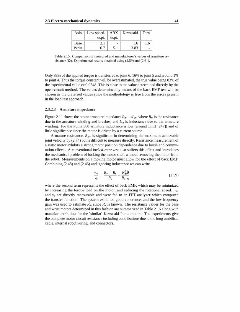
2.3Electro-mechanicaldynamics 41
Axis Low speed. ARX Kawasaki Tarnexpt. expt.
Base 2.1 - 1.6 1.6Wrist 6.7 5.1 3.83 -
Table2.15: Comparisonof measuredandmanufacturer's valuesof armaturere-sistance(Ω). Experimentalresultsobtainedusing(2.59)and(2.61).
Only 83%of theappliedtorqueis transferredto joint 6, 16%to joint 5 andaround1%to joint 4. Thusthetorqueconstantwill beoverestimated,thetruevaluebeing83%oftheexperimentalvalueor 0 0548.This is closeto thevaluedetermineddirectlyby theopen-circuitmethod.Thevaluesdeterminedby meansof thebackEMF testwill bechosenasthe preferredvaluessincethemethodologyis free from theerrorspresentin theloadtestapproach.
2.3.2.3 Armatur e impedance
Figure2.11showsthemotorarmatureimpedanceRm sLm, whereRm is theresistancedueto the armaturewinding andbrushes,andLm is inductancedueto the armaturewinding. For the Puma560armatureinductanceis low (around1mH [247]) andoflittle significancesincethemotoris drivenby a currentsource.
Armatureresistance,Rm, is significantin determiningthe maximumachievablejoint velocityby (2.74)but is difficult to measuredirectly. Resistancemeasurementofa staticmotorexhibits a strongmotorpositiondependencedueto brushandcommu-tationeffects. A conventionallocked-rotor testalsosuffersthis effect andintroducesthemechanicalproblemof locking themotorshaftwithout removing themotor fromtherobot. Measurementson a moving motormustallow for theeffect of backEMF.Combining(2.48)and(2.45)andignoringinductancewecanwrite
vm
vs
Rm Rs
Rs
K2mθ
Rsτm(2.59)
wherethe secondtermrepresentstheeffect of backEMF, which maybeminimizedby increasingthe torqueload on the motor, and reducingthe rotationalspeed. vm
and vs are directly measurableand were fed to an FFT analyzerwhich computedthe transferfunction. The systemexhibited goodcoherence,andthe low frequencygain wasusedto estimateRm sinceRs is known. Theresistancevaluesfor the baseandwrist motorsdeterminedin this fashionaresummarizedin Table2.15alongwithmanufacturer's datafor the 'similar' KawasakiPumamotors. The experimentsgivethecompletemotorcircuit resistanceincludingcontributionsdueto thelongumbilicalcable,internalrobotwiring, andconnectors.

42 Modelling the robot
It is possibleto simultaneouslyestimateRm andLm usingthebackEMF constantalreadydetermined,andtime recordsof motorterminalvoltage,currentandshaftan-gle. Firstit is necessaryto computethemotorvoltagecomponentdueonly to armatureimpedance
vZm vm Kmˆθ (2.60)
by subtractingtheestimatedbackEMF. Equation(2.48)mayberewritten in discrete-timeARX form as
VZm Rm Rs ImLm
T1 z 1 Im
Rm RsLm
TLm
Tz 1 Im (2.61)
andaparameteridentificationtechniqueusedasfor thetorqueconstantcase.For joint6 theidentificationresultsin estimatesof Rm 5 1Ω andLm 0 83mH. Theinduc-tanceis of a similarorderto thatreportedby Tarnet al. [247], but theresistanceesti-mateis somewhat lower thanthatobtainedusingthelow-speedtestdescribedabove.Giventheapproximationsinvolvedin thelow-speedtest,(2.59),theresultfrom (2.61)is to bepreferred,althoughtheexperimentalprocedureis lessconvenient.
2.3.2.4 MATLAB simulation model
Themodelof armaturemotionincludingfriction andstictionthathasbeendevelopedis asimplifiedversionof thatproposedby Hill [117] for simulationof radio-telescopeantennae.Like a gearedrobot theseantennaehave high levels of friction relativeto maximumtorque. The armaturemotion is modelledby a non-linearsystemwithtwo statescorrespondingto the motor beingstationaryor moving. If the motor isstationarytheappliedtorquemustexceedthestictiontorquefor motionto commence.If thespeedfalls below a thresholdε thenthemotorentersthestationarystate.
Ω 0 if stationary1
Js B τ τC if moving(2.62)
Hill' s approachis somewhat moresophisticatedandrequiresa fixedstepintegrationalgorithm.Thealgorithmis implementedasaMATLAB `S-function'andis availablefor usein SIMULINK [182] models.It workssatisfactorilywith thebuilt in variable-length-stepintegrationroutines.
2.3.3 Curr ent loop
TheUnimatecurrentloopis implementedin analogelectronicsonthesocalledanalogservoboard,oneper axis, within the controllerbackplane.A block diagramof the

2.3Electro-mechanicaldynamics 43
VIdEm
RA
6.06 VIM RS
05 105 107
Motor Impedance
VoltageFB
ShuntCurrentFB
k1 4 1059 7 105 107
0 2 6 106
PowerampCompensator
1Lms Rm
Im
Eb
Figure2.13:Block diagramof motorcurrentloop. Eb is themotorbackEMF, Vmmotorterminalvoltage,andRA theamplifier's outputimpedance.
Unimatecurrentloop is shown in Figure 2.13. The transferfunction of the blockmarkedcompensatorwasdeterminedfromanalysisof schematics[255] andassumingidealop-ampbehaviour. Thecompensatorincludesanintegrator, addinganopen-looppoleattheorigin in ordertoachieveType1 systemcharacteristicsin currentfollowing.Theremainingdynamicsareat frequencieswell beyondtherangeof interest,andwillbe ignoredin subsequentmodelling. The voltagegain of the block markedpoweramplifier, k, hasbeenmeasuredasapproximately 50.
Currentfeedbackis from ashuntresistorin serieswith themotor, seeFigure2.11.Theshuntsare0 2Ω and0 39Ω for thebaseandwrist joints respectively. Thehighforward path gain, dominatedby the compensatorstage,resultsin the closed-loopgain,Ki, beinggovernedby thefeedbackpath
KiImVId
16 06 Rs
(2.63)
The measuredfrequency responseof the joint 6 currentloop is shown in Figure2.14,andthe magnitudeandphaseconfirmtheanalyticmodelabove. Theresponseis flat to 400Hz which is consistentwith Armstrong's [22] observation that currentstepsto the motorsettlein lessthan500µs. Theuseof a currentsourceto drive themotoreffectively eliminatesthemotor's electricalpole from theclosed-looptransferfunction.
Themeasuredcurrent-looptransconductanceof eachaxisis summarizedin Table2.16. The gainsareconsistentlyhigherthanpredictedby (2.63),but no more than

44 Modelling the robot
101
102
103
104
-12
-10
-8
-6
-4
-2
Freq (Hz)
Mag
(dB
)
101
102
103
104
-300
-250
-200
Freq (Hz)
Pha
se (
deg)
Figure2.14:Measuredjoint 6 current-loopfrequency responseIm VId .
Joint Ki A V immax A
1 -0.883 8.832 -0.877 8.773 -0.874 8.744 -0.442 4.425 -0.442 4.426 -0.449 4.49
Table2.16: Measuredcurrent-looptransconductances andestimatedmaximumcurrent. The measurementis a lumpedgain from the DAC terminalvoltagetocurrent-loopoutput.
expectedgiven the toleranceof componentsusedin the variousgain stages15. Themaximumcurrentin Table2.16is estimatedfrom themeasuredtransconductanceandthemaximumcurrent-loopdriveof vid 10V.
15Thecircuitry usesonly standardprecision,10%,resistors.

2.3Electro-mechanicaldynamics 45
10-1
100
101
102
5
10
15
20
25
30
35
Freq (Hz)
Mag
(dB
)
Model
Figure2.15: Measuredjoint 6 motorandcurrent-looptransferfunction,Ωm VId ,with fittedmodelresponse.
2.3.4 Combinedmotor and current-loopdynamics
The measuredtransferfunction betweenmotor currentandmotor velocity for joint6 is givenin Figure2.15,alongwith a fitted transferfunction. The transferfunctioncorrespondsto a linearizationof thenon-linearmodelof Figure2.10for a particularlevel of excitation.Thefittedmodelis
Ωm
VId
24 431 4
rad s V (2.64)
whichhasa poleat 5Hz. FromFigure2.10and(2.63)themodelresponseis givenby
Ωm
VId
KmKi
Jef f s Bef f(2.65)
whereJef f andBef f arethe effective inertia andviscousfriction due to motor andtransmission.Fromthemeasuredbreakfrequency andArmstrong'sinertiavaluefromTable2.13theestimatedeffective viscousfriction is
Bef f 33 10 6 31 4 1 04 10 3N m s radm (2.66)

46 Modelling the robot
Substitutingthesefriction andinertiavaluesinto equation(2.65)gives
Ωm
VId
KmKi
33 10 6 s 1 04 10 3 (2.67)
Equatingthenumeratorwith (2.64),andusingknown Ki from Table2.16leadsto anestimateof torqueconstantof 0 060which is similar to thevaluedeterminedearlierin Table2.14.
Theestimatedeffective viscousfriction is significantlygreaterthanthemeasuredvalueof 37 10 6N m s rad from Table2.12. This is a consequenceof the linearidentificationtechniqueusedwhich yieldsthe 'small-signal'response.Theeffectiveviscousfriction includesa substantialcontribution dueto Coulombfriction particu-larly at low speed.Coulombfriction may be linearizedusingsinusoidalor randominputdescribingfunctionsgiving aneffective viscousdampingof
Bef f BkτC
2σθ(2.68)
whereσθ is theRMSvelocity, andk 1 27(sinusoidal)or k 1 13(random).The large-signalresponsemaybemeasuredby stepresponsetests,andthesein-
dicatea muchhighergain— approximately200rad s V. From (2.65)the DC gainis
KmKi
Bef f(2.69)
which leadsto anestimateof effective viscousfriction of 126 10 6N m s rad. Asexpectedat the higherspeed,this estimateis closerto themeasuredviscousfrictioncoefficient of Table2.12.
2.3.4.1 Curr ent and torque limits
Maximummotorcurrentprovidesanupperboundon motortorque.Whenthemotoris stationary, thecurrentis limited only by thearmatureresistance
imaxva
Rm(2.70)
whereva is the maximumamplifier voltagewhich is 40V for the Puma. From thearmatureresistancedatagivenin Table2.15it canbeshown thatthemaximumcurrentgivenby (2.70)is substantiallygreaterthanthelimit imposedby thecurrentloopitself.Maximumcurrentis thusa functionof thecurrentloop,not armatureresistance.Thesustainedcurrentis limited furtherby thefuses,or circuit breakers,whichareratedat4A and2A for thebaseandwrist motorsrespectively. Thefuselimits arearoundhalfthemaximumachievableby thecurrentloop.

2.3Electro-mechanicaldynamics 47
Joint τI l oop τ f use
1 120 562 200 973 110 524 22 105 22 106 21 10
Table2.17: Maximumtorque(load referenced)at currentloop andfusecurrentlimits. All torquesin N.m.
Usingmaximumcurrentdatafrom Table2.16,andknown motortorqueconstants,themaximumjoint torquescanbecomputed.Table2.17shows thesemaximafor thecaseof currentlimits dueto thecurrentloopor fuse.
2.3.4.2 Back EMF and amplifier voltagesaturation
A robotmanipulatorwith gearedtransmissionnecessarilyhashighmotorspeeds,andthushigh backEMF. This resultsin significantdynamiceffectsdueto reducedmotor torqueandamplifier voltagesaturation. Sucheffects areparticularlysignif-icant with the Pumarobot which hasa relatively low maximumamplifier voltage.Figure2.16shows theseeffectsvery clearly— maximumcurrentdemandis appliedbut theactualmotorcurrentfalls off rapidly asmotorspeedrises.Combining(2.52)and(2.48),andignoringmotorinductancesincesteadystatevelocity andcurrentareassumed,thevoltageconstraintcanbewrittenas
θKmτ
KmRT va (2.71)
whereRT is the total circuit resistancecomprisingarmatureresistance,Rm, andam-plifier outputimpedanceRa. Rising backEMF alsodiminishesthe torqueavailablefrom theactuatorduringacceleration
τavail va θKmKm
RT(2.72)
However during deceleration,backEMF works to increasemotor currentwhich isthenlimitedby thecurrentloopor fuse.Whenthefrictional torqueequalstheavailabletorque
τC θB va θKmKm
RT(2.73)

48 Modelling the robot
0 0.2 0.4-150
-100
-50
0
Time (s)
Sha
ft an
gle
(rad
m)
0 0.2 0.4-600
-400
-200
0
200
qd_max = -439.5
Time (s)
Sha
ft ve
loci
ty (
radm
/s)
0 0.2 0.4-6
-4
-2
0
2
I_mean = -0.2877
I_max = -4.312
Time (s)
Mot
or c
urre
nt (
A)
Figure2.16:Measuredmotorandcurrentloopresponsefor astepcurrentdemandof VId 10. Motor angle,velocityandcurrentversustimeareshown. qmax is thesteadystatevelocity, and Imean is the steadystatecurrent. The finite rise-timeon thecurrentstepresponseis dueto theanti-aliasingfilter used.Thesamplinginterval is 5ms.
thejoint velocity limit dueto amplifiervoltagesaturation
θvsatvaKm RTτC
RT B K2m
(2.74)
is attained.Armatureresistance,RT , andfriction, serve to lowerthis valuebelow thatdueto backEMF alone.Thecorrespondingmotorcurrentis
ivsatBva KmτC
RT B K2m
(2.75)
Experimentswereconductedin which themaximumcurrentdemandwasappliedto eachcurrentloop,andthemotorpositionandcurrenthistoryrecorded,asshown inFigure2.16.Theinitial currentpeakis approximatelythemaximumcurrentexpected

2.3Electro-mechanicaldynamics 49
Joint Measured Estimatedθvsat ivsat θvsat ivsat
1 120 2.1 149 3.22 163 0.26 165 1.33 129 0.42 152 1.74 406 0.56 534 0.845 366 0.39 516 0.756 440 0.29 577 0.51
Table2.18:Comparisonof experimentalandestimatedvelocity limits dueto backEMF andamplifier voltagesaturation.Velocity andcurrentlimits areestimatedby (2.74)and(2.75)respectively. Velocity in radm/sandcurrentin Amps.
from Table2.16,but falls off dueto voltagesaturationasmotorspeedrises.Withoutthis effect the motorspeedwould ultimatelybelimited by friction. Table2.18com-parescomputedmaximumjoint velocitiesandcurrentswith theresultsof experimentssimilar to thatleadingto Figure2.16.Theestimatesfor θvsat aregenerallyhigherthanthemeasuredvalues,perhapsdueto neglectingtheamplifieroutputresistance(whichhasnot beenmeasured).Measurementsfor joints 2 and3 arecomplicatedby theef-fectof gravity whicheffectively addsaconfiguration-dependenttorquetermto (2.72).To counterthis, gravity torquewascomputedusing(2.36)and(2.35)andthecorre-spondingcurrentsubtractedfrom thatmeasured.At voltagesaturation,thecurrentisgenerallyaround30%of themaximumcurrentachievableby thepoweramplifier.
2.3.4.3 MATLAB simulation
A completeSIMULINK modelof themotorandcurrentloopis shown in Figure2.17.This modelis a stiff non-linearsystemandis thusvery slow to simulate.Thehigh-orderpolesdueto motorinductanceandthecurrent-loopcompensatorarearound300timesfasterthanthedominantmechanicalpoleof themotor. Non-linearitiesareintro-ducedby voltagesaturationandCoulombfriction. Thereducedordermodel,Figure2.18,hassimilar non-linearcharacteristicsbut doesnot have thehigh-orderpoles,ismuchfasterto integrate,andis to bepreferredfor simulationpurposes.Increasingthevalueof Rm above that in Table2.15allows themodelto moreaccuratelypredictthesaturationspeedandcurrent. This couldbeconsideredasallowing for the currentlyunmodeledamplifieroutputimpedance.
2.3.5 Velocity loop
Like thecurrentloop, theUnimatevelocity loop is implementedin analogelectronicson theanalogservoboard.A block diagramof thevelocity loop is shown in Figure

50 Modelling the robot
Model of Puma joint 1
2
Torquedisturb
−
+
+Sum2
wTau
Eb
Im
3
Vel
2
Im
1
PosAmplifiervoltage
limit
1/s
Integrator
6.06
Inputgain
.2
Shunt
++
Sum1
.22
Ebconst
.22
Torqconst
1
300e−6s+.0016
Mech
1
0.00283s+4.5
Elec
+−
Sum
−1e5
s
I.loopcompensator
1
Currentdemand
Coulomb
Figure2.17:SIMULINK modelMOTOR: joint 1 motorandcurrent-loopdynamics.
Joint 6 using friction data from pcc 27/6/93
Model of Puma joint 1
2
Torquedisturb
++
Sum2
wTau
Eb
Im
3
Vel
2
Im
1
PosAmplifiervoltage
limit
1/s
Integrator
.0534
Ebconst
.0534
Torqconst
++
Sum
1
Currentdemand
−1/9
1/Rm
+−
Sum3
9
Rm
.449
Iloop 1/(Js+B)
Coulomb1
Figure2.18:SIMULINK modelLMOTOR:reducedordermodelof joint 6 motorandcurrent-loopdynamics.
2.19,and includesthe motor andcurrentloop blocksalreadydiscussed.The gainsKgain andKvel aresetby trimpotsR31(GAIN) andR29(VELOCITY) respectively oneachanalogservo board.TheUnimationPumadoesnot usea tachometerto measuremotorvelocity. Instead,avelocitysignalis synthesizedfromthetriangularoutputsig-nal from themotor's incrementalencoderby ananalogdifferentiatoranda switchingnetwork.Thegainof thesynthetictachometerhasbeenexperimentallydeterminedtobe
KtachVΩm
Ωm34 10 3V s radm (2.76)
with someincreasein gainat frequenciesbelow 2Hz. FromFigure2.19the closed-loop transferfunctionfor themotor, currentandvelocity loop is
Ωm
VΩd
KgainKiKm
Js B KiKmKgainKvelKtach
B
(2.77)

2.3Electro-mechanicaldynamics 51
+ θm1
s
1
Js B+Ki Km
Kgain
KtachKvel
ΩmτmImVIc
VΩm
VΩd
electronictachometer
rotordynamics
poweramplifier
+
Figure2.19:Velocity loopblockdiagram.
It is desirablethat B B in order that the closed-loopdynamicsareinsensitive toplantparametervariation,but in practicethisis notthecase.TheadjustablegainsKgain
andKvel provide interactingcontrolof theDC gainandclosed-looppolelocation.Themeasuredtransferfunctionbetweenmotorvelocityandvelocitydemandfor joint 6 isgivenin Figure2.20andthefittedmodelis
Ωm
VΩd
11 91486
radm s V (2.78)
Observe thatthemechanicalpoleof themotorat5Hz hasbeen'pushedout' to nearly25Hz by the actionof the velocity loop. Substitutingknown numericvalues16 into(2.77)resultsin thetransferfunction
Ωm
VΩd
12 8137
radm s V (2.79)
andcompareswell with themeasuredresult(2.78).Again,this transferfunctionrep-resentsthesmall-signalresponseof thesystem.
The large signalgain for eachaxis hasalsobeendeterminedexperimentallybyproviding a stepdemandto thevelocity loop andmeasuringtheresultantslopeof thejoint positionversustime curve. Theseresults,summarizedin Table2.20,arehighlydependenton the way the particularanalogvelocity loop hasbeen' tuned', asgivenby (2.77). It canbeseenthat joint 2 hasa significantlyhighervelocity gainthantheothers,probablyto compensatefor its muchhighergearreductionratio.
A SIMULINK modelof the velocity loop is shown in Figure2.21. This modelmakesuseof themotorandcurrent-loopmodelLMOTOR developedearlier.
16ThegainsKgain 2 26,andKvel 1 75 weredeterminedby measuringthetransferfunctionbetweenadjacentpointsin thecircuitry with anFFT analyzer. Kvel 6 06Kvel whereKvel 0 288is thegainof thetrimpotR29.

52 Modelling the robot
10-1
100
101
102
-5
0
5
10
15
20
25
30
Freq (Hz)
Mag
(dB
)
Model
Figure2.20: Measuredjoint 6 velocity-looptransferfunction,Ωm VΩm, with fit-tedmodelresponse.Phasedatais notshown but is indicativeof asignreversal.
2
vel
++
Velocityerror
6
Kgain(R30)
1
Vd1
thetaVelocity demand
(volts)Motor angle
radm
2
Tau_d
Disturbance torqueinput (Nm@motor)
Motor velradm/s
lmotor
Motor
Mux
Mux
DeMux
Demux
-K-
tacho
-6.1
Feedbackgain
Unimate velocity loop
.28
Kvel'(R29)
Errorsaturation
Figure2.21:SIMULINK modelVLOOP: motorvelocity loop.
2.3.6 Position loop
Thepositionloopis implementedonadigital servoboard— oneperaxis.Thisboardutilizesa 6503,8-bit microprocessorclockedat 1MHz to closeanaxispositionloopat approximately1kHz, andalsoto executecommandsfrom thehostcomputer[56].Positionfeedbackis fromincrementalencoders,whosecharacteristicsaresummarizedin Table2.19,fitted to themotorshafts.Theanalogcontrolsignal,vDAC, is generated

2.3Electro-mechanicaldynamics 53
Cur.loop
Digitaltacho
Ωm
VIm
VId
DACPositionloop
Counter
ed
em
S1
VDAC M
RS
ImPoweramp
Encoder
S2S2
Digital servo board Analog servo board
Lead/lag+velocityloop
Figure2.22: Unimationservo positioncontrol mode. The switch S2 routestheoutputof theDAC to theleadcompensatorandvelocity loop.
Joint Encoderresolution Counts/motorrev. Counts/radl
1 250 1000 99652 200 800 137273 250 1000 85484 250 1000 121025 250 1000 114476 250 500 6102
Table2.19:Puma560joint encoderresolution. Notethatjoint 6 is generallyrunin 'divideby two mode',sothattheencodercountmaintainedby thedigital servoboardis half thenumberof actualencodercounts.This is necessarysincejoint 6canrotatethrougha rangeof morethan216 counts.
by a12-bitDAC with abipolaroutputvoltagein therange-10V to 9.995V anddrives,via ananalogcompensationnetwork,theanalogvelocitydemand.Theoverall controlsystemstructureis shown in Figure2.22.
A block diagramof thepositionloop is givenin Figure2.23. Thedigital controlloop operatesat a sampleinterval of Tservo 924µs. The encoderdemand,ed, isprovided by the hostcomputerat intervalsof 2N Tservo whereN is in the range2 to7 resultingin hostsetpointintervalsof approximately4.5, 7, 14, 28, 56 or 112ms.Themicroprocessorlinearly interpolatesbetweensuccessive positionsetpoints,at theservo rate. At thatsamerate,the microprocessorimplementsthe fixed-gaincontrol

54 Modelling the robot
+ θm
313 31.3( )1( )
1.3 37.3( )373( )
10ed
Kenc
-
em
VΩd10
2048
Velocityloop
D/AZOHinterpolator Lead
compensator
Tservo
VDAC
Figure2.23:Block diagramof Unimationpositioncontrol loop.
law17
vDAC10
2048ed em (2.80)
whereed is the desiredencodervaluefrom the interpolator, andem is the measuredencodercount.Thiscontrollaw hasbeenverifiedby disassemblyof themicroproces-sor'sEPROM andby measuringthetransferfunctionVDAC em. Theoutputvoltageisa velocitycommandwhichis conditionedby a phaseleadnetwork
1 337 3373
(2.81)
soasto increasetheclosed-loopbandwidth.Thegainof 1 3 wasdeterminedby analy-sisof thecircuit, but themeasuredgainfor joint 6 wasfoundto be1 13. A switchableintegralactionstage
I s10 if therobotis moving, or313 31 3
1 if therobotis 'on station'(2.82)
is enabledby themicroprocessorwhentheaxis is within a specifiedrangeof its set-point. Integral action booststhe gain at low frequency, increasingthe disturbancerejection.
Thetransferfunctionof theleadnetwork(2.81)andintegralstage(2.82)introduceagainof around11 3 beforethevelocityloop. Thevelocitycommandvoltage,VΩd , islimited by thecircuit to therange 10V, sotheDAC voltagemustin turn belimitedsuchthat
vDAC10
11 3(2.83)
17Sincethedigital controllerhasafixedgain,loopgainis adjustedby thevelocity-loopgaincontrol.

2.3Electro-mechanicaldynamics 55
Joint ω vDAC θmax θmax θvsat
radm/s/V radm/s radm/s1 -101 89 74%2 -318 281 172%3 -90.2 80 62%4 -366 324 80%5 -235 208 57%6 -209 185 42%
Table2.20: Measuredstep-responsegains,ω vDAC, of velocity loop. Stepmag-nitudewasselectedso asto avoid voltagesaturationeffects. Thesegainvaluesincludetheeffect of theposition-loopleadnetworkandswitchableintegral/gainstage. θmax is the estimatedmaximumvelocity due to the velocity loop whenvΩd 10V. Rightmostcolumnis ratioof velocity limits dueto velocity loopandvoltagesaturationeffects.
This limits the usablevoltagerangefrom the DAC to only 0 88V — that is only9%of theavailablevoltagerange,andgivesaneffective resolutionof lessthan8 bitson velocity demand.This saturationof the velocity-loopdemandvoltageis readilyapparentin experimentation.Frommeasuredvelocity-loopgains,ω vDAC, shown inTable2.20andknowledgeof maximumDAC voltagefrom (2.83),themaximumjointvelocitiescanbedetermined.Thesemaximaaresummarizedin Table2.20alongwiththeratioof velocitylimits dueto velocityloopandvoltagesaturationeffects.For mostaxesthemaximumdemandedjoint velocity is significantlylessthanthelimit imposedby voltagesaturation.Theonly exceptionis joint 2 which,asobservedearlier, hasanabnormallyhighvelocity-loopgain.
Root-locusdiagramsfor the joint 6 positionloop areshown in Figures2.24and2.25. For the casewith no integral actionthe dominantpole is on the realaxis dueto theopen-looppoleat theorigin moving towardthecompensatorzero,resultingina closed-loopbandwidthof 32Hz. Thecomplex polepair hasa naturalfrequency of57Hz anda dampingfactorof 0.62.With integralactionenabledthedominantmodeis a lightly dampedcomplex polepairwith anaturalfrequency of around1.2Hz andadampingfactorof 0.25.
A SIMULINK modelof thepositioncontrolleris shown in Figure2.26.Thestruc-ture of the switchableintegral actionstageis somewhat differentto Figure2.23butmorecloselyrepresentstheactualcontroller, in particularwith respectto 'bumpless'switchingof the integrator. This model is usedextensively in later chapterswheninvestigatingthebehaviour of visual-loopclosedsystems.

56 Modelling the robot
0.5 0.6 0.7 0.8 0.9 1-0.25
-0.2
-0.15
-0.1
-0.05
0
0.05
0.1
0.15
0.2
0.25
Real AxisIm
ag A
xis
Figure2.24:Root-locusdiagramof positionloopwith no integral action.
0.85 0.9 0.95 1
-0.06
-0.04
-0.02
0
0.02
0.04
0.06
Real Axis
Imag
Axi
s
Figure2.25:Root-locusdiagramof positionloopwith integral actionenabled.
2.3.6.1 Host current control mode
The Unimatedigital servo boardalsoallows the motor currentto be controlleddirectly by the host. In this modethe DAC outputvoltageis connecteddirectly tothe currentloop asshown in Figure2.27. The DAC is updatedwithin Tservo of thesetpointbeinggiven.Thismodeis usefulwhenthehostcomputerimplementsits ownaxiscontrolstrategy.
2.3.7 Fundamentalperformancelimits
A summaryof therobot'sperformancelimits is givenin Table2.21.Thevelocitylim-its aredueto backEMF andvoltagesaturation,givenpreviously in Table2.18. The

2.3Electro-mechanicaldynamics 57
2
Integralenabled
1
Kp
DeMux
Demux
Mux
Mux
0
Constant++
Sum1
abs(u)<10
On-station?
Encoderquantization
-K-
Encoder
vloop
Vel. loop
13(s+37.3)(s+373)
Lead network
ZOHSetpoint
interpolate
Switch
-303(s+1)
Integral
1
Motorangle(rad)
1
Encodersetpoint
-K-
DAC
+-
Sum
-10
Gain
em
e d
VDAC
Figure2.26:SIMULINK modelPOSLOOP:Unimationdigital positioncontrolloop.
Cur.loop
Digitaltacho
Ωm
VIm
VId
DAC
Positionloop
Counter
ed
em
S1
VDAC M
RS
Im
Poweramp
Encoder
S2S2
Digital servo board Analog servo board
Lead/lag+velocityloop
Figure2.27:Block diagramof Unimationservocurrentcontrolmode.TheswitchS2 is usedto routethe hostsetpointdirectly to thecurrent-loopdemandvia theDAC, bypassingthevelocity loopandleadcompensator.
torquelimits arederivedfrom thefuse-limitedcurrentandtorqueconstantdatafromTable2.14. Accelerationlimits areestimatedfrom the torquelimits, maximumnor-malizedlink inertia from Table2.10,andarmatureinertiafrom Table2.13.Notethatthe velocity andaccelerationmaximaaremutuallyexclusive — maximumaccelera-tion canbeachievedonly at zerovelocity or duringdeceleration.Maximumvelocityoccurswhenachievableaccelerationis zero.

58 Modelling the robot
Joint Motor referenced Loadreferenced
θ τ θ θ τ θ1 120 0.91 840 1.92 56 132 163 0.91 3200 1.51 97 303 129 0.97 3000 2.40 52 554 406 0.14 3800 5.34 10 495 366 0.14 4000 5.09 10 556 440 0.11 3700 5.74 10 48
Table2.21:Summaryof fundamentalrobotperformancelimits.
2.4 Significanceof dynamic effects
Whennumericparametersaresubstitutedinto thesymbolictorqueexpressionsfromSection2.2.2 it becomesclear that the varioustorquecontributionsvary widely insignificance.For example,the accelerationof joint 6 exertsa very small torqueonjoint 2 comparedto the gravity load on that axis. While considerableliteraturead-dressesdynamiccontrolof manipulators,lessattentionis paidto thesignificance,orrelative magnitude,of the dynamiceffects. In muchearly work the velocity termswereignored,partly to reducethecomputationalburden,but alsoto acknowledgethereality thataccuratepositioningandhigh speedmotionareexclusive in typical robotapplications.Severalresearchers[119,153,164]have investigatedthedynamictorquecomponentsfor particularrobotsandtrajectories.Unfortunatelythesignificanceof thetorquecomponentsis highly dependentuponbothrobotandtrajectory. Khosla[153]for examplefoundthat,for theCMU DD-II arm,inertiatorquesdominate.
RecentlyLeahy [162] hasproposedstandardtrajectoriesfor the comparisonofmodel-basedcontrollersfor thePuma560robot18. Figure2.28showsthetorquecom-ponentsfor the proposedtesttrajectory. Leahy's minimumjerk trajectoryalgorithmwasnot availableso a seventhorderpolynomialwasusedinstead,andthis seemstohave resultedin marginally higherpeakvelocitiesandaccelerations.It is clearthatfriction, gravity andinertiatorquesaresignificant.Anothersignificantfactoris torquelimitation dueto voltagesaturation.Figure2.28showstheavailabletorquecomputedasa functionof joint velocity, andthis limit is clearlyexceededin themiddleof thetrajectory. The proposedtrajectoryis perhapstoo closeto the robot's performancelimit to beof useasa benchmark.
Symbolic manipulationof the dynamicequationsprovidesanotherway to gain
18Unfortunatelytheproposedstandardis expressedin termsof startandfinish joint angles,but doesnotspecifythejoint angleconventionused.Howeverstudyof earlierworkby Leahy[164] indicatesthatheusesthe conventionof Lee [166]. Anotherunfortunateomissionwasthe“minimum jerk” trajectorygeneratoralgorithmused.

2.4Significanceof dynamic effects 59
0 0.5 1 1.5-20
-10
0
10
20
30
40
50
60
Time (s)Jo
int 1
torq
ue (
Nm
)
A
TF
V
I
G
0 0.5 1 1.5-40
-30
-20
-10
0
10
20
30
40
Time (s)
Join
t 2 to
rque
(N
m)
T
A
G
VI
F
0 0.5 1 1.5-30
-25
-20
-15
-10
-5
0
5
10
Time (s)
Join
t 3 to
rque
(N
m)
A
A
T
F
I
G
V
Figure2.28: Breakdown of torquecomponentsfor Leahy's proposedtesttrajec-tory. Joints1, 2 and3 shown down the page. The curvesaremarked;T totaltorque,F friction, G gravity, I inertia,andV velocity terms.ThecurvemarkedAis theavailabletorquedueto amplifiervoltagesaturation,(2.72),andfusecurrentlimit.

60 Modelling the robot
Rank Joint1 Joint2 Joint31 0 6916S2q2 37 23C2 8 744S23
2 1 505C22 q1 4 182q2 0 6864q3
3 1 943S32C2S2 q1 q2 8 744S23 0 2498C4
2 q3
4 1 301C22C3
2 q1 0 7698S3 q2 0 3849S3q2
5 1 637C32C2S2 q1 q2 0 3849S3 q3 0 1688S4
2 q3
Rank Joint4 Joint5 Joint61 0 1921q4 0 1713q5 0 1941q62 0 02825S23S4S5 0 02825C23S5 03 0 001244S4S5 q3 0 02825C4C5 S23 04 0 001244S3S4 S5 q2 0 001244C4C5 q3 05 0 001244S4S5 q2 0 001244C4C5 S3 q2 0
Table2.22: Rankingof termsfor joint torqueexpressions.Computedat 20%peakaccelerationand 80% peakvelocity. Motor armatureinertia is included.Coefficientsareshown to 4 figures.
insight into thesignificanceof variousdynamiceffects. After numericalsubstitutioninto the symbolicequationsthe termsin the torqueexpressionscomprisea numericcoefficient multiplied by a functionof manipulatorstatevariables.Themagnitudeofthe coefficient is relatedto thesignificanceof that term to the total torque. Velocitytermscontaineithera velocity squaredor a productof velocitiesandmaybesignifi-cantdespitea smallcoefficient. Theprocedureintroducedhereinvolvessettingjointvelocitiesandaccelerationsto nominalvaluesprior to rankingthe magnitudeof theterms.Thenominalvalueschosenare20%of themaximumacceleration,and80%ofthemaximumvelocityasgivenin Table2.21.Table2.22showsthe5 mostsignificantdynamictermsfor eachtorqueexpressionat the nominalvelocity andacceleration.As expected,gravity rankshighly for joints 2 and3, followedby inertia. Joint3 hasanoff-diagonalinertial componentindicatingsomecouplingwith joint 2. Joint1 hassignificantCorioliscouplingwith joint 2 andto alesserextentjoint 3. Thewrist jointsaredominatedby inertia,with gravity andinertialcouplingeffectsoneandtwo ordersof magnitudedown respectively.
2.5 Manipulator control
2.5.1 Rigid-body dynamicscompensation
In conventionalmanipulatorcontrol, for instancethe standardUnimatecontroller,eachaxis is independentlycontrolled,andtorquesdueto inertial coupling,Coriolis,

2.5Manipulator control 61
-
+
ArmInversearm
Kp
Kv
q..
d
q.d
qd
q'..
d+
+
+
+
-
q
q.
Figure2.29:Computedtorquecontrolstructure.
-
+
Arm
Inversearm
Kp
Kv
q..
d
q.d
qd
q'..
d
+
+
+
-
q
q.
τ ff
++
Tfb
Tff
Figure2.30:Feedforwardcontrolstructure.
centripetalandgravity effectsaretreatedasdisturbances.Gearinghelpsto reducetheconfigurationdependenceof somedynamiceffects,andalsoreducesthemagnitudeofdisturbancetorquesat themotor. Thequalityof trajectorytrackingis directly relatedto the disturbancerejectioncapabilityof the axis servo. However givenknowledgeof themanipulator'sequationsof motion,inertialparameters,andmanipulatorstateitis possibleto computethe joint torquerequiredto follow a trajectory, andexplicitlycounterall thedisturbancetorques.
The two major forms of control incorporatingmanipulatordynamicsthat have

62 Modelling the robot
beenproposed[69] are:
1. Computedtorquecontrol, shown in Figure2.29. The torquedemandfor theactuatorsis
Q M q Kv qd
q Kp qd
q qd
C q q q F q G q (2.84)
whereKp is thepositiongain,andKv thevelocity gain,or dampingterm. Theinversedynamicsare'in the loop' andmustbeevaluatedeachservo interval,althoughthe coefficientsof M , C, andG could be evaluatedat a lower rate.Assumingidealmodellingandparameterization,theerrordynamicsof thelin-earizedsystemare
e Kve Kpe 0 (2.85)
wheree qd q. Theerrordynamicsof eachaxisareindependentanda func-tion only of the chosengain matrices. In the caseof modelerror therewillbecouplingbetweenaxes,andtheright-handsideof (2.85)will bea non-zeroforcing function.
2. Feedforwardcontrol,shown in Figure2.30, linearizesthedynamicsabouttheoperatingpointsqd, qd andqd, by providing thegrosstorques
Q M qd
qd
C qd
qd
qd
F qd
G qd
Kv qd
q Kp qd
q
(2.86)whereKp is thepositiongain,andKv is thevelocitygain,or dampingterm.Theinversedynamicsarenot 'in theloop' andcanbeevaluatedata lowerrate,Tf f ,thanthe error feedbackloops,Tf b. Again assumingideal linearizationof theplant,theerrordynamicsaregivenby
M qd
e Kve Kpe 0 (2.87)
whichareseento bedependentuponmanipulatorconfiguration.
In eachcasethe positionandvelocity loopsareonly requiredto handlemodellingerrorsanddisturbances.Both techniquesrequireaccuratedeterminationof manipu-lator stateandin particularjoint velocity. Commonly, robotshave only joint positionsensorssovelocity mustbeestimated.Khosla[151] describesa “leastsquaresdigitalfilter” for this purpose,but otherreportson model-basedcontrolexperimentsdo notdiscussthis issue.
Thereis relatively little experimentalevaluationof thedynamiccontrol of robotmanipulators.Onereasonis the lack of manipulatorsfor which theserigid-bodydy-namiceffectsaresignificant,thoughthis situationhaschangedover the last5 years.Most commercialrobotsarecharacterizedby high gearratios,substantialjoint fric-tion, and relatively low operatingspeed— thus independentjoint control suffices.

2.5Manipulator control 63
Gravity loadingis commonlycounteredby introducingintegralactionto thepositionloopwhennearthedestination.
A numberof studieshave investigatedtheefficacy of thecontrolstrategies(2.84)and (2.86) for the Puma560 and variousdirect drive robots. In generalthe per-formancemetric usedis high-speedposition tracking error. Valavanis, Leahy andSaridis[257] reportedon computedtorquecontrol for a Puma600robot,andfoundtheperformanceinferior to individualjoint control.Thediscussionis notspecific,butit wouldseemproblemsin modelling,andthelow sampleratemayhavecontributedtotheresult.They concludethatfor sucha highly gearedmanipulator, gravity andfric-tion overwhelmthejoint interactionforces.Laterwork by Leahyetal. [161,162,165]concludesthattrackingperformanceimproveswith thecompletenessof thedynamicmodelwhich ultimately includesfriction, velocity termsandpayloadmass. Leahyalsofindsthatcomputedtorquecontrolis superiorto feedforwardcontrol.
As alreadyalludedto, it is possibleto computethefeedforwardtorqueat a lowerratethanthe feedbacktorque. Leahy[162] investigatesthis for feedforwardtorquecontrol andfinds acceptableperformancewhenTf f is up to eight timeslongerthanTf b. Accuracy is increasedif thefeedforwardtorqueis computedat thefeedbackrate,but with the feedforwardtorquecoefficients,M q
d, C q
dq
d, andG q
d, evalu-
atedat thelowerrate.Theseapproachescanreducetheonlinecomputationalburden.Sharkey et al. [228] provide a strongerreasonfor sucha control strategy. They ar-guethat theinertial compensationneednot becomputedat a ratebeyondthedesiredclosed-loopbandwidth. Inertial parameteruncertaintymeansthat high-bandwidthcontrolshouldberestrictedto local joint feedbacksoasto controlunmodeleddynam-ics. High-bandwidthinertial compensation,in conjunctionwith poorinertial models,wasfoundto couplenoisebetweenaxes,leadingto poorcontrol.
In the lastdecade,with theavailability of high-torqueactuators,a numberof ex-perimentaldirect-driverobotshave beenbuilt to exploit thepotentiallygreaterperfor-manceachievableby eliminatingthecomplex transmission.Severalstudieshavecom-paredthe two control strategiesdescribed,andKhosla[152] concludes,like Leahy,that thecomputedtorqueschemegivesslightly betterperformancethanfeedforwardcontrol whenmodellingerrorsarepresent.If an exact modelis availablethenbothschemeswould give thesameresults.Khoslaalsofoundthat the off-diagonaltermsin the manipulatorinertia matrix weresignificantfor the CMU DD-II arm. An etal. [11] evaluateda spectrumof controlstrategiesfor theMIT SLDD Arm, includingindependentjoint control,gravity feedforward,andfull dynamicsfeedforward.Theyconcludethat feedforwardcontrol significantlyimprovesfollowing accuracy at highspeed,andthatmodelaccuracy wasimportant.Furtherwork [10] findsno significantdifferencebetweenfeedforwardandcomputedtorquecontrol.
A moreradicalapproachis to designthe manipulatorso as to simplify the dy-namics. The MIT 3DOF direct drive arm [287] usedclever mechanicaldesigntoensurethat the manipulator's inertia matrix is diagonalandconfigurationinvariant.

64 Modelling the robot
This is achieved by placing all actuatorsremotelyand transmittingthe torqueviaa transmission,eliminatingthe reactiontorquestransmittedbetweenadjacentlinks.This approachsimplifiesdynamiccontrol, andensuresuniformity of responseoverthework volume.TheMinnesotadirectdrivearm[145] is staticallybalancedto elim-inategravity forces.Theprincipalbenefitsaccruenot somuchfrom simplificationofthedynamicsexpressions,but from theuseof smaller(andlighter)motorsdueto theeliminationof steadystateholdingtorques.
2.5.2 Electro-mechanicaldynamicscompensation
As seenfrom Section2.4 friction andvoltagesaturationeffectsaresignificant. Thelattercannotbecompensatedfor — it is a fundamentalconstraintin motionplanning[17]. However a numberof strategies have beenproposedto counterfriction andinclude[43]:
high-gaincontrol loopsto reducethe effect of non-linearities,but with limit-cyclesasa possibleconsequence
addinga high frequency 'dither' signalto the torquecommand,at theexpenseof possiblyexciting high orderstructuraldynamics,andpossiblefatigueof ac-tuatorsandbearings;
compensationby non-linearfeedforwardof friction torque,which requiresanaccuratemodelof thefrictional characteristicsof thejoint.
CanudasDeWit [43] describestheeffect of underandover compensationof esti-matedfriction onsystemstability for PDjoint controllers.Hethendescribesanadap-tive compensationschemewhich estimatestheunknown frictional characteristics.Amajor sourceof difficulty is noise-freedeterminationof low velocity. He proposesa combinedfeedbackandfeedforwardcompensatorwherethe feedforwardtorqueiscomputedfrom measuredvelocityaboveavelocitythreshold,andfrom desiredveloc-ity below thethreshold.Experimentalresultsconfirmedtheoperationof theproposedalgorithm. The controllersdescribedin Sections8.1 and8.2 usethis techniqueforfriction compensation.
2.6 Computational issues
Model-baseddynamiccontrol,eitherby computedtorqueor feedforward,requirestherapid computationof the manipulator's inversedynamics.Throughthe 1980smuchliteraturewasdevoted to ways of computingthe inversedynamicssufficiently faston microprocessorhardwareto allow online control. The approacheshave includedDSPdevices[138], parallelprocessing,tablelookup[209], andspecialarchitectures[18,168,172,208].

2.6Computational issues 65
Many of thereportsseemtohavefocussedonatargetof 6-axistorquecomputationtimein around1msbut this levelof performancemaybeunwarranted.Luhetal. [177]indicatea servo rateof at least60Hz is requiredandPaul [199] suggestsa servo rateof 15 timesthehigheststructuralresonance.However thecoefficientsof thedynamicequationsdo not changerapidly sincethey area function of joint angleandmaybecomputedat a fraction of the rateat which the servo equationsareevaluated[201].Sharkey etal. [228] gofurtherandcontendthatit maybedisadvantageousto computerigid-bodydynamicsata highratesincethedynamicmodelis unlikely to beaccurateat thosehigh frequencies.Computationof therigid-bodydynamicsfor all 6 joints isalsounnecessarysincethe dynamiceffectsaremostsignificantfor the baseaxesasshown in Table2.22.Anothertrendin the1980swastheincreasingpower of generalpurposesymbolicalgebrapackages,enablingresearchersto readily manipulatethevery complex dynamicequationsof motion. Symbolicsimplification,in conjunctionwith modernmicroprocessors,offersanattractive alternative to specializedhardwarearchitectures.Thenext sectionsreview work in theareasof parallelcomputationandsymbolicsimplificationandthencontrastthetwo approaches.
2.6.1 Parallel computation
Lathrop [159] providesa good summaryof the computationalissuesinvolved andsomeapproachesto parallelism.A significantproblemin usingmultiple processorsis schedulingthecomponentcomputationaltasks.This difficult problemis tackledinmany differentways,but is essentiallyan 'of f-line' processthat needbe doneonlyonce.Importantissuesin parallelizationinclude:
Level of decomposition.Is the minimum scheduledcomputationa dynamicvariable,matrixoperationor scalarmultiplication?As theparallelismbecomesmore fine grained,interprocessorcommunicationsbandwidthwill becomealimiting factor.
Utilization profile or load balancing. It is desirableto keepall processorsasfully utilizedaspossible.
The 'speedup' achieved, that is, the executiontime ratio of the multiproces-sor implementationto thesingleprocessorimplementation.Thespeed-upcannever exceedthenumberof processors,andtheratio of speed-upto numberofprocessorsis someindicationof the benefitgained,or efficiency of multipro-cessing.
Luh [176] demonstratedhow six processorscouldbeusedto achieve a speed-upof 2.64 for computationof the manipulatorinversedynamics. A “variablebranch-and-bound”techniquewasdevelopedto schedulethe computingtasks.NighamandLee [194] proposean architecturebasedon six 68020processors,with the parallel
66 Modelling the robot
computationsscheduledmanually. Integerarithmeticis proposed,andwith 16.7MHzdevicesa time of 1.5ms is predicted,but issuessuchassharedresourcecontentionor synchronizationarenotdiscussed;nor is theimprovementover singleCPUperfor-mancegiven. Khosla[150] alsodescribesa manualapproachto schedulingthecom-putationsonto8 processorsfor theNE formulation,to achieve an81%timereduction(speed-upof 5.3). KasaharaandNarita [144] describeanautomaticapproachto thenp-hardproblemof multiprocessorscheduling.They show thedecompositionof thedynamicsof a six-axisrevolute robot into 104computationaltasks,anda maximumspeed-upof 3.53for four CPUs.
An alternateapproachis to partitiontheprobleminto oneaxisperprocessor. Un-fortunatelythe recursive natureof the RNE computationis suchthat the inward re-cursionfor link i cannotbe initiateduntil the outwardrecursionfor links i 1 to n,andinward recursionfor links n to i 1, have beencompleted.However the inter-actionforce andmomentfrom the inward recursioncanbe predictedfrom previousvalues,andthis allowseachjoint processorto operateindependently. Vuskovic [263]investigatestheerrorsintroducedby prediction;zero-orderpredictiongaveacceptableresults,andtheerror is shown to reducewith sampleinterval. First-orderpredictionwas lesssuccessful.A speed-upfactor of 6 over a single processorwasachieved,without theneedfor complex off-line taskscheduling,andin fact theprocessorscanoperatecompletelyasynchronously. Yii et al. [286] alsodescribea zero-orderpredic-tivesystem,but providenoexperimentalresults.
Lathrop[159]usesadirectedgraphto representtheRNEformulation,with groupsof parallelprocessorsateachnode.Conventionalandsystolicpipelinedstructuresareproposedwith a speed-upof two ordersof magnituderequiring180'simple' matrix-vectorprocessorsfor the6-axiscase.Thisapproachis thenextendedto anew parallelimplementationwhich hasO log2n costrequiring637matrix-vectorprocessorsfor6 axes.
Hashimotoetal. [112] describeaparallelformof theRNEequationsderivedfromanalysisof datadependency graphs.For n joints thecomputationcanbedividedinton approximatelyequalparalleltasks.Laterwork [113] discussestheimplementationof this algorithmfor 3-axisdynamiccontrol of a Puma560 with threetransputers,achieving a dynamicscomputationtimeof 0.66ms.
2.6.2 Symbolicsimplification of run-time equations
Symbolicexpansionof theequationsof motionhasbeenpreviouslydiscussedin Sec-tion 2.2.2,but thesum-of-productform is tooexpensive for run-timeevaluationsincetheinherentfactorizationof theRNEformhasbeenlost,andsymbolicre-factorizationis prohibitively expensive. A far betterapproachis to retainfactorsduringsymbolicevaluation.In thiswork whenever anintermediateexpressiongrowsto becomeasumof morethanoneproducttermthenthatexpressionis replacedby a singlenew vari-

2.6Computational issues 67
Method 3-axis 6-axisMul Add Factors Mul Add Factors
Generalsolution 402 345 852 738Symbolically simplified byMAPLE
238 108 45 538 254 106
Symbolic simplified byMAPLE after parametervaluesubstitution
203 59 39 358 125 93
ARM closedform 461 352ARM recursive form 224 174IzaguirreandPaul [131] 331 166Leahy[164] 304 212
Table 2.23: Operationcount for Puma560 specificdynamicsafter parametervaluesubstitutionandsymbolicsimplification.
able,which is equatedto the previous expression. Table 2.23 shows the operationcountfor this factoredsymbolicrepresentationfor aPuma560,aswell asthenumberof factorssogenerated.Theoperationcountis considerablylessthanthegeneralformgivenin Table2.2.Substitutingnumericvaluesfor inertialparameters,many of whicharezero,reducestheoperationcountstill further.
ARM hasbeenused[192] to generatecustomizedcomputationsfor both directandinversedynamics.Theinversedynamicscanbein closedor recursive form, thelatterbeingmostadvantageousfor highernumbersof joints. Theresultsof ARM arecomparedwith theresultsobtainedusingthewriter'sMAPLE programin Table2.23.TheMAPLE resultscomparevery favorablywith thoseof ARM for thecomparableclosedform solution.ARM' s factoredrecursive form hasnotbeenimplementedwithMAPLE. Anothersymbolicapproachgeneratescomputationallyefficientformsof theinertia andvelocity termsvia a Lagrangianformulation[131]. Written in LISP, theprogramsreada manipulatorparameterfile, andwrite 'C' functionsto computetheM , C andG matricesasfunctionsof manipulatorstate.
2.6.3 Significance-basedsimplification
Asshown in Table2.22thetermsin thetorqueexpressionsvarygreatlyin significance.This canbeseenclearly in Figure2.31which shows a histogramof the distributionof thesecoefficient magnitudesfor the Puma560's joint 1 torqueexpression. Themediancoefficient magnitudeis nearly four ordersof magnitudebelow that of thegreatestcoefficient. In thissectionweinvestigatethepossibilityof 'culling' theterms,keepingonly thosethatcontribute 'significantly' to the total joint torque. Using the

68 Modelling the robot
−5 −4.5 −4 −3.5 −3 −2.5 −2 −1.5 −1 −0.5 00
50
100
150
200
250
300
N
log10 |αij|
Figure2.31: Histogramof log10 α1 j coefficient magnitudefor τ1, normalizedwith respectto the greatestcoefficient, for the Puma560. The medianvalueis-3.67.
nominalvelocityandaccelerationvaluesasin Section2.4thetorqueexpressionsweretruncatedatcoefficientmagnitudelessthan5%and1%of thegreatestcoefficient. Thenumberof remainingtermsfor eachaxisaresummarizedin Table2.24.A comparisonof moreelaborateculling methodsis givenin [53].
To investigatetheeffect of culling on accuracy a simpleMonte-Carlostyle sim-ulationwasconducted.Error statisticswerecollectedon the differencebetweenthefull andtruncatedtorqueexpressionsfor N randompointsin manipulatorstatespace.The joint angleswereuniformly distributedin the joint anglerange,while velocityandaccelerationwerenormally distributedwith the 2σ valuesequatedto the limitsfrom Table2.21. Theseresultsarealsosummarizedin Table2.24. Truncationto 5%introducesnegligible errors,exceptfor joint 2. A goodcompromisewould appeartobeculling to 1% significancefor joint 2 and5% for all others.At the5% level only4%of thetermsremainin thetorqueexpression.Onlinetorquecomputationbasedonthesetruncatedtorqueexpressionsis usedin thecontrollerdescribedin Section8.2.
2.6.4 Comparison
To placesomeof theseefforts in context, theexecutiontimesof theRNEformulationfor a 6-axis Puma560 are given in Table 2.25. The matrix numericexamplesbythe authorwerewritten in 'C' in a straightforwardmanner, while the symbolicallysimplifiedexamplesweregeneratedautomaticallyby MAPLE with someminor code

2.6Computational issues 69
Joint Norig 5%significanceNterms τd στd max∆τ
1 1145 162 0.0027 0.0978 0.45992 488 8 0.0814 6.6640 22.72003 348 19 0.0218 0.6881 2.56604 81 3 -0.0002 0.0188 0.08475 90 4 -0.0003 0.0217 0.08916 18 2 0.0000 0.0010 0.0032
2170 199
Joint Norig 1%significanceNterms τd στd max∆τ
1 1145 333 -0.0013 0.0251 0.10242 488 36 0.0158 0.7514 2.84703 348 39 -0.0041 0.1420 0.59074 81 30 -0.0001 0.0027 0.01345 90 36 -0.0002 0.0031 0.01656 18 2 0.0000 0.0010 0.0032
2170 476
Table2.24: Significance-based truncationof the torqueexpressions.This showstheoriginalnumberof termsin theexpression,andthenumberaftertruncatingto5%and1%of themostsignificantcoefficient.Also shownarethemean,standarddeviationandmaximum(all in N.m)of theerrordueto truncation,computedover1000randompointsin manipulatorstatespace.All torquesarelink referenced.
massagingperformedby sed scripts.Table2.25shows that, for thesameprocessor,the factoredsymbolicform executesapproximately3 timesfasterthanthe numericmatrix form of (2.12) to (2.25). This ratio of 3 would be expectedfrom examiningthe operationcountssummarizedin Table2.23. The fairly 'ordinary' singleboardcomputerfor robot control in this work, a 33MHz 68030, is able to computethetorquefor thefirst 3 axesin only 800µs.
In ordertocomparescalarandparallelimplementationsacomputationalefficiencymetricis proposed
ηn 106
N fclockT(2.88)
wheren is the numberof axes, N the numberof processors,fclock the CPU clockrate,andT theexecutiontime. Clock rateis includedto enablecomparisonbetweenscalarandparallelimplementationson thesameCPU type,but is not meaningfulincomparisonacrossprocessortypes.
Table 2.26 comparestwo reportedparallel implementationswith scalarresultsgeneratedby the authorfrom Table 2.25. The parallel implementationsareshown

70 Modelling the robot
Processor Approach Axes Year Time(µs)
PDP-11/45[177] assembler, RNE 6 1982 4500Sun3/60 'C' generalRNE 6 1988 13400µPD77230DSP[138] assembler, generalRNE 6 1989 550Sun4/20(SLC)† 'C' generalRNE 6 1990 1630T800x 3 [112] Occamparallelprocessing 3 1989 660T80525MHz 'C' + symbolicsimplification 3 1989 570T80525MHz 'C' + symbolicsimplification 6 1989 114068030+6888233MHz 'C' + symbolicsimplification 6 1989 158068030+6888233MHz 'C' + symbolicsimplification 3 1989 795Sun4/20(SLC) ” 6 1990 548Sun4/20(SLC) ” 3 1990 362SparcStation10 ” 6 1993 65
Table2.25:Comparisonof computationtimesfor Puma560equationsof motionbasedon RNE formulation. The given year is an indicationonly of when theparticularcomputingtechnologywas first introduced. Thosemarkedwith a †were benchmarkedby the writer, using the GNU C crosscompiler v2.2.3 for68030,gcc v2.4.5 for the Sparcand Helios C v2.05 for the transputer, T805.Compileroptimization,-O, wasenabledin all cases.
to makepooruseof thecomputinghardware.This is fundamentallybecausethey areusingadditionalhardwareto performarithmeticoperationswhich canbeeliminatedoff-line. It canbeconcludedthatoff-line symbolicmanipulation,high-level languagesand state-of-the-artcomputersprovide a simpleand powerful meansof computingmanipulatordynamicsat a sufficient rate. Thegenerationof symbolicallysimplifiedrun-timecodein 'C' from a Denavit-Hartenberg parameterfile executesin lessthan15s on a Sun SparcStation2. Specializedhardwareor parallelsoftwarewith theirinherentlongdevelopmenttimesmustnow beseenasanunattractiveapproachto theonline computationof manipulatordynamics.The off-line computationaleffort de-votedto schedulingparallelcomputation[144,176,194], describedin Section2.6.1,wouldperhapshave beenbetterdevotedto symbolicsimplification.

2.6Computational issues 71
Approach CPU fclock N T n η(MHz) (ms)
Nigham&Lee 68020 16.7 6 1.5 6 39.9Corke 68030 33 1 2.0 6 119Hashimoto T800 20 3 0.66 3 76Corke T805 25 1 3.8 0.57 211
Table2.26:Comparisonof efficiency for dynamicscomputation. Writtenby theauthor, seeTable2.25. Clockspeedof 20MHz is assumedonly.

72 Modelling the robot

Chapter 3
Fundamentalsof imagecapture
This chapterintroducessomefundamentalaspectsof imageformationandcapturethat areparticularlyrelevant to visual servoing. Camerasareoften treatedasblackboxeswith a coupleof adjustmentrings, but beforean imagebecomesavailable ina framestorefor computeranalysisa numberof complex, but frequentlyoverlooked,transformationsoccur. Theseprocessingstepsaredepictedin Figure3.1andincludeillumination, lens,sensor, cameraelectronicsanddigitizer, andeachwill introduceartifactsinto thefinal digital image.Particularlyimportantfor visualservoingarethetemporalcharacteristicsof thecamera,sincethecamera's shutteractsasthesamplerin a visualcontrolloop.
This chapterwill systematicallyexaminetheprocessof imageformationandac-quisition,generallyoverlooked,prior to it beingdigitally processed.The effectsofeachstageareexaminedanda detailedmodelbuilt up of thecameraandimagedig-itizing system. A particularcamera,Pulnix TM-6, and digitizer, DatacubeDIGI-MAX [73], areusedasconcreteexamplesfor modeldevelopment,but aretypical ofCCDcamerasanddigitizersin general.
3.1 Light
3.1.1 Illumination
Light is radiantenergy with a capacityto producevisualsensationandphotometryisthatpartof thescienceof radiometryconcernedwith measurementof light. Radiantenergy striking a surfaceis calledradiantflux andis measuredin watts.Radiantfluxevaluatedaccordingto its visualsensationis luminousfluxandis measuredin lumens.Theratio of luminousflux to radiantflux is luminositymeasuredin lumens/watt.The
73

74 Fundamentalsof imagecapture
lensCCDsensor
analogcameraelectronics
digitizerFramestore
analogvideosignal(CCIR)
10MHzfilter
sample
quantization
+
timing
Illuminance
reflectionfrom scene
timing
DC restoregainoffset
sync
sigsyncseparator
camera
data
address
sync
Figure3.1: Stepsinvolvedin imageprocessing.
photopic1 luminositycurve for a 'standard'observer is shown in Figure3.2.The luminousintensityof a sourceis theluminousflux perunit solidangle2 mea-
suredin lumens/sror candelas.Somecommonphotometricunits aregivenin Table3.1.For apointsourceof luminousintensityI theilluminanceE falling normallyontoa surfaceis
EIl2 lx (3.1)
where l is the distancebetweensourceand the surface. Outdoorilluminanceon abright sunny day is approximately10,000lx, whereasoffice lighting levels aretypi-cally around1,000lx. The luminanceor brightnessof a surfaceis
Ls Ei cosθnt (3.2)
1Theeye's light-adaptedresponseusingthe conephotoreceptorcells. Thedark adapted,or scotopic,responseusingtheeye'smonochromaticrodphotoreceptorcellsis shiftedtowardthelongerwavelengths.
2Solidangleis measuredin steradians,asphereis 4πsr.

3.1Light 75
350 400 450 500 550 600 650 700 750 8000
100
200
300
400
500
600
700
Wavelength (nm)
Lum
inos
ity (
lum
ens/
W)
Figure3.2: CIE luminositycurve for the'standardobserver'. Peakluminosityis673lumens/Wat awavelengthof 555nm(green).
Quantity Unit Symbol Equivalentunits
Luminousflux lumen lmSolidangle steradian srLuminousintensity candela cd lm/srIlluminance lux lx lm/m2
Luminance nit nt lm/m2/sr
Table3.1: CommonSI-basedphotometricunits.
whereEi is theincidentilluminanceatanangleθ to thesurfacenormal.
3.1.2 Surfacereflectance
Surfacesreflectlight in differentwaysaccordingto surfacetextureandwavelength— thetwo extremesarespecular('glossy') anddiffuse('matte') reflectionasshownin Figure3.3. A specular,or mirror like, surfacereflectsa ray of light at anangle,θr ,equalto theangleof incidence,θi. A diffusesurfacescattersincidentlight in all direc-tions. A Lambertiansurfaceis a perfectlydiffusingsurfacewith a matteappearance

76 Fundamentalsof imagecapture
incomingray
incomingray
Specularreflection
Diffusereflection
θ
θ
θi r
r
Figure3.3: Specularanddiffusesurfacereflectance.Lengthof theray is propor-tional to luminousintensity.
andhasconsistentluminanceirrespective of viewing angle3. Theluminousintensityof a surfacepoint is
I rEcosθr cd (3.3)
whereE is theilluminance,andr thesurfacereflectivity (0 r 1). Typical reflec-tivitiesare;whitepaper0.68,photographicgrey card0.18,anddarkvelvet0.004.Theluminanceor 'brightness'of theLambertiansurfaceis
Lrπ
Ent (3.4)
whichis independentof θi andθr . In practice,realsurfacesareacombinationof theseextremesandlight is reflectedin a lobecenteredabouttheangleθr θi .
3.1.3 Spectralcharacteristicsand color temperature
Many illumination sources,suchas incandescentlampsandthe sun,have radiationspectrathatcloselyapproximatea blackbodyradiator4 ata temperatureknown asthecolor temperature of thesource.Thecolor temperatureof solarradiationis 6500K,anda standardtungstenlampis 2585K.
Figure 3.4 comparessolarand tungstenspectraand alsoshows the spectralre-sponseof thehumaneye anda typical silicon CCD sensor. The peakfor a tungstenlamp is in the infra-red and this radiationserves to heatratherthan illuminate the
3Luminousintensity decreaseswith anglefrom the normal,but so too doesthe apparantareaof thelight-emittingsurfacepatch.
4Thesolarspectrumatgroundlevel is substantiallymodifiedby atmosphericabsorption.

3.1Light 77
300 400 500 600 700 800 900 1000 11000
0.1
0.2
0.3
0.4
0.5
0.6
0.7
0.8
0.9
1
Wavelength (nm)
Eye
CCD
Tungsten
Sun
Figure3.4: Blackbodyemissionsfor solarandtungstenillumination. The pho-topic responseof the humaneye and that of a typical silicon CCD sensorareshown for comparisonpurposes.
Symbol Name Value
C1 3 741844 10 16W m2
C2 1 438835 10 2m Kσ Stefan-Boltzmannconstant 5 669572 10 8W m2 K4
h Planck'sconstant 6 626197 10 34J sk Boltzmann'sconstant 1 38062 10 23J Kc Speedof light in vacuum 2 99792459 108m s
Table3.2: Relevantphysicalconstants.
subject— only a small fraction of the radiationis emittedin the visible spectrum.Radiationfrom fluorescenttubescannotbeapproximatedby ablackbodycurve,sincethe light is due to fluorescenceof variousphosphors,eachwith a narrow spectralemission.
The radiationspectrumof a blackbodyat temperatureT asa function of wave-
78 Fundamentalsof imagecapture
length,λ, is givenby Planck's radiationformula
M λ2πhc2
λ5 ehc kλT 1
whereh is Planck's constant,k is Boltzmann's constant,andc is the speedof light.Theequationis frequentlywritten in theform
M λC1
λ5 eC2 λT 1
whereC1 andC2 areconstantsgivenin Table3.2. Theunitsof M areW m3 whichis interpretedaswattsemittedperunit areaperunit wavelength.The integral of thisfunctionis thetotalpowerradiatedperunit area
Mtot
∞
0M λ dλ σT4W m2
whereσ is the Stefan-Boltzmannconstant. The wavelengthcorrespondingto peakemissionis givenby Wien'sdisplacementlaw
λmax0 0028978
Tm
TheSI valuesof therelevantphysicalconstantsaresummarizedin Table3.2.For a given radiationspectrum,M λ , the correspondingluminousflux canbe
obtainedby
φtot
∞
0M λ K λ dλ
whereK λ is luminosity in lumensper watt. The energy of a photonis given byPlanck'sequation
Ephot λhcλ
J
andthusthephoton-fluxdensityis
nphot
∞
0
M λEphot λ
dλ (3.5)
∞
0
λM λhc
dλ photonsm2 (3.6)
Thusthenumberof photonsperlumenfor a givenradiationspectrumis
∞
0
λM λhc
dλ∞
0M λ K λ dλ
photons lm

3.2Imageformation 79
Source Photons/lumen
Tungstenlampat2885K 2 0 1016
Tungstenlampat3200K 1 8 1016
Tungstenlampat5600K 1 4 1016
RedLED at670nm 1 6 1017
Table3.3: Photonsperlumenfor sometypical illuminants.
Y
Z
P
f
−f
lensplane
inverted image
object
O−zi
oz
Figure3.5: Elementaryimageformation,showing aninvertedreal imageof theobject.
Resultsfor a numberof standardilluminants aresummarizedin Table3.3. Thesevaluescanbeusefulin analyzingthesensitivity of CCD sensorswhich aretypicallyquotedin termsof electronsperlux for anominatedstandardilluminant.Knowing thechargewell capacityof thephotosite,in electrons,allowsusto estimatetheluminousflux over thephotositerequiredfor saturation.
CCD sensorsaresensitive to infra-redradiationbut sensitivity expressedin elec-trons/luxcannotquantifythissinceelectronsaregeneratedby infra-redphotonswhichdo notcontributeto luminousflux. Infra-redfiltersarefrequentlyfitted to CCD cam-erasto prevent saturationfrom infra-red radiation,particularlywhenworking withtungstenlamps.Infra-redradiationreducesimageclarity sincethelongerwavelengthsarefocusseddifferentlyby thelensandsuchphotonscausehigherpixel cross-talkinthesensor, seeSection3.3.
3.2 Imageformation
The elementaryaspectsof imageformationwith a simplelensareshown in Figure3.5. ThepositiveZ-axisis thecamera's optical axis. Thevariablesarerelatedby the

80 Fundamentalsof imagecapture
lenslaw1zo
1zi
1f
(3.7)
wherezo is the distanceto the object,zi the distanceto the image,and f the focallength. For zo f a real invertedimageis formedat zi f (limzo ∞ zi f ). For anobjectat infinity thefilm or solid statesensoris placedon thefocal planeat z f .For nearobjectstheimageis formedbehindthefocalplane,sothelensmustbemovedout of thecamerain orderto focustheimageon thefilm or sensor.
Theimageheight,yi , is relatedto theobjectheight,yo, by themagnification
Myi
yo
ff zo
fzo
(3.8)
which is negative,sincezo f , representingtheimageinversion.Notethatmagnifi-cationdecreasesastheobjectdistance,zo, increases.
Thef -numberof a lensis thedimensionlessquantity
F f d (3.9)
whered is thediameterof thelens.f -numberis inverselyrelatedto thelight gatheringability of the lens. To reducelight falling on the imageplane,theeffective diametermaybereducedby a mechanicalapertureor iris, which increasesthe f -number. Illu-minanceat the imageplaneis reducedby F2 sinceit dependson light gatheringarea— to increaseilluminanceby a factorof 2, the f -numbermustbereducedby a factorof 2 or 'one stop'. Theminimumf -numberis markedona lens,andis relatedto itslight gatheringcapability. Thef -numbergraduationson theaperturecontrolincreaseby afactorof 2 ateachstop.An f -numberis conventionallywrittenin theform f/1.4for F 1 4.
The horizontaland vertical subtendedanglesof the coneof view, or anglesofview, aregivenby
θH 2tan 1 W2 f
(3.10)
θV 2tan 1 H2 f
(3.11)
whereW andH arerespectively thehorizontalandverticaldimensionsof thecamera'sactive sensingarea.Standard35mm film is 24mm 36mm, whereasa CCDsensoris around10mm 10mm. Table3.4comparestheanglesof view for differentfocallengthlensesandsensorsizes.Clearly for therelatively smallCCD sensor, thefieldof view is muchnarrower comparedto film. Frequentlythesemi-anglesof view aregivenwhicharehalf theanglesof view givenabove. Theangleof view is amaximumwhenthelensis focussedat infinity.

3.2Imageformation 81
f (mm) PulnixCCD 35mmfilmθH θV θH θV
8 44 33 132 11325 15 11 72 51
Table3.4: Anglesof view for PulnixCCDsensorand35mmfilm. Computedforvariouslensesandwith CCDdimensionstakenfrom Table3.8
In practice,compoundlensesareused,comprisinga numberof simplelensele-mentsof differentshapesfabricatedfrom differentglasses.This reducesthesizeofthe lensandminimizesaberrations,but at the expenseof increasedlight lossduetoreflectionat eachopticalinterface.
3.2.1 Light gathering and metering
Theilluminanceon theimageplaneof acamera,Ei , is givenby
EiπLT cos4θ
4F2 M 1 2 lx (3.12)
whereL is thesceneluminance,T thetransmissionefficiency of thelens,M themag-nification, andθ is the anglefrom the optical axis to the imageplanepoint5. Thecos4 θ termmodelsthe fall off in illuminanceaway from theopticalaxisof the lens.For largeobjectdistance M 1 2 1 andtheilluminanceat thesensoris indepen-dentof objectdistance6.
A lightmeteris a device with fixed optics that measuresthe radiantflux fallingon a sensorof known areaA. By suitablechoiceof spectralcharacteristicthesensoroutputcanbeinterpretedasluminousflux, φ. Photographersemploytwo methodsoflight measurement:
1. Incidentlight measurementsmeasuretheilluminanceof thescene,andaretakenbyplacingthemeterin frontof thesubjectaimedatthecamera.Theilluminanceis givenby
EsφA
(3.13)
Theluminanceof thesceneis computedusing(3.4)andanassumedreflectivityof 18%7
Ls0 18
πφA
(3.14)
5Thiseffect is pronouncedin shortfocal lensessincemax θ W 2 f whereW is thesensorwidth.6This may seemcounterintuitive, but asobjectdistanceincreasesthe imagesize is reducedasis the
spatialintegralof luminousflux.718% 2 2 5 andcorrespondsto thegeometricmeanof the5 stopreflectancerangeof ' typical' scenes.
82 Fundamentalsof imagecapture
2. Reflectedlight measurementsmeasuretheluminanceof thescenedirectly, andaretakenby placingthemeternearthecameraaimedat thescene.Theillumi-nationmeasuredby thesensor(3.13)is relatedto thesceneluminanceby (3.12)sothat
Ls4F2
πTφA
(3.15)
whereF andT areknown characteristicsof thelightmeter'soptics.
The two typesof measurementaresimply differentscalingsof the lightmetersensoroutput. A lightmetergenerallyreturnsthe logarithmof luminancecalledexposurevalue,or EV, which is relatedto luminanceby
L k2EV (3.16)
The calculationdials on a lightmeterarea circular slideruleimplementingequation(3.12)which relatesexposuretime to aperturefor a givensceneluminanceandfilmsensitivity or 'speed'.Exposure of thefilm or sensoris
e EiTe (3.17)
in unitsof lux.s,whereEi is theilluminanceandTe is theexposuretime.TheISOfilmspeed,S, is determinedfrom theexposurenecessaryto “discerniblyfog” thefilm
S0 8e
(3.18)
The factor k in (3.16) is typically around0 14 andresultsin the film exposurebeing'centered'within its dynamicrange8.
An alternativeapproach,usedby photographers,is touseaspot-readinglightmeterto measurethebrightestanddarkestregionsof thesceneseparately, andthenmanuallycomputetherequiredexposure.
3.2.2 Focusand depth of field
Maintainingfocusover a widerangeof camera-objectdistancesis a non-trivial prob-lem whenthecamerais mountedon theendof a robot. Theoptionsareto establisha largedepthof field or usea lenswith servo controlledfocus. The latterapproachhasa numberof disadvantagessincesuchlensesaregenerallyheavy andbulky, havelimited adjustmentrates,relativeratherthanabsolutefocussetting,andtargetdistancemustbesomehow determined.
8Theexposurecomputedon the basisof film speedis only sufficient to “discerniblyfog” thefilm. Agoodphotographrequiresa higherexposure,which is achievedby calculationsbasedon a fractionof therealluminance.

3.2Imageformation 83
500 1000 1500 2000 2500 3000 3500 4000 4500 50000
1000
2000
3000
4000
5000
6000
7000
8000
9000
10000
Focus setting z_f (mm)
Foc
us r
ange
(m
m)
Figure3.6: Depthof field boundsfor 8mm (solid)and25mmlenses(dashed)atf/1.4. Circle of confusionis 25µm ( 3 pixels) in diameter. Thevertical line atzf 1820mmis thesingularityin zF at thehyperfocaldistance.
Depthof field is therangein objectdistanceoverwhichthelenscanformanimagewithoutsignificantdeterioration.This is definedsuchthattheimageof a pointsourceobject is a circle of diametera or smaller— the so calledcircle of confusion. Theboundsof theacceptablefocusrangearegivenby
zN zfzf
M faF 1
(3.19)
zF zfzf
M faF 1
(3.20)
wherezN andzF arethenearandfar boundsof theacceptablefocusrange,andzf isthe focussettingof the lens. The locusof nearandfar boundsfor a rangeof focussettingsis shown in Figure3.6.Whenthelensis focussedat thehyperfocaldistance
zf f 1f
aF(3.21)

84 Fundamentalsof imagecapture
the depthof field extendsfrom half the hyperfocaldistanceto infinity. Rearranging(3.19)and(3.20)givesthefocusandaperturesettingfor a specifiedfocusrange
zf2zNzF
zN zF(3.22)
Ff 2 zF zN
2azNzF(3.23)
The f 2 termin (3.23)meansthat longerfocal lengthlenseswill requirea very largef -numberin order to maintaina given depthof field, andwill thushave very littleilluminationontheimageplane.
For 35mmfilm thecircleof confusiondiameteris typically takenas25µm [250],andfor a CCDarrayis thepixel-to-pixel spacing[82] (seeTable3.8). Largedepthoffield is achieved by usinga small aperture,but at the expenseof light falling on thesensor. Therequirementfor largedepthof field andshortexposuretime to eliminatemotionblur bothcall for increasedambientillumination, or a highly sensitive imagesensor.
3.2.3 Imagequality
In practicetheimageformedby a lensis not ideal. Lensesusedfor imagingareusu-ally compoundlensescontainingseveralsimplelensesin orderto achieve a compactoptical system. Imperfectionsin the shapeor alignmentof the simple lensesleadsto degradedimagequality. Non-idealitiesincludeaberrationswhich lead to imageblur, andgeometricdistortionswhichcausetheimageto fall in thewrongplace.It isimportantto matchthe lenswith thesensorsizeused9 , sincelensesaredesignedtominimizeeffectssuchasgeometricdistortionandvignettingonly over thesensororfilm area.
3.2.3.1 Aberrations and MTF
Aberrationsreduceimageclarity by introducingblur. This leadsto reducedcontrastonfine imagedetail.Commonaberrationsinclude[28]:
Sphericalaberration, coma, astigmatismandfield curvature which introducevariationsin focusacrossthescene.
Chromaticaberrationsdueto differentwavelengthsof light beingfocussedatdifferentdistancesfrom thelens.
Vignetting,whereimagebrightnessfalls off at theedgesof thefield of view dueto theeffect of thelensbarrel.
9Lensesaretypically manufacturedfor 1 2, 2 3 and1inchsensors.

3.2Imageformation 85
Diffractiondueto theaperture,which will reducethe definitionof the image.Theimageof apoint sourcewill beanAiry pattern10 andtheminimumsepara-tion atwhich two point sourcescanbediscernedis
d 2 4λF (3.24)
whereλ is thewavelengthof the illumination (λ is often takenas555nm, theeye's peaksensitivity). Dif fractioneffectsare thusmostpronouncedat smallapertureor high f -number.
Theeffectof aberrationscanbereducedby closingtheaperturesincethis restrictsthelight raysto asmallcentralregionof eachopticalelement.However this increasesthemagnitudeof diffractioneffects.It is generallydesirableto operatebetweenthesetwo extremes,wherethemagnitudesof thetwo effectsareapproximatelyequal.
In orderto quantify imagesharpness,the relationshipbetweencontrastandres-olution is important. This canbe consideredas the magnitudeof a spatialtransferfunction which is generallyreferredto as the modulationtransferfunctionor MTF.Aberrationsresult in MTF roll-off at high spatialfrequency. MTF is normally ex-pressedasa percentageof theuniformillumination response(or DC gain).TheMTFis themagnitudeof thenormalizedFourier transformof the line spreadfunction, thedistribution of intensityalonga line orthogonalto the imageof a line of negligiblewidth. A relatedmeasurementderived from the spatialsquarewave responseis thecontrasttransferfunctionor CTF. Usefulspatialresolutionis typically givenin lines,determinedasthehighestdistinguishableline pitch in aresolutiontestchart.Thespa-tial resolutionof the completeimagingsystemis obtainedby multiplying the MTFdueto thelens,sensorandandanalogelectronics,andis discussedfurtherin Sections3.3.2and3.5.5.
The MTF at the spatialNyquist frequency is relatedto the rise distance11 of animageof a sharpedgeby
MTF fs 21N
(3.25)
whereN is the numbersof pixels for the imageintensityto rise from 10% to 90%[121].
3.2.3.2 Geometricdistortion
Unlike aberration,geometricdistortion leaves the imagesharpbut causesit to fallin thewrongplace[28]. Geometricdistortionsareclassifiedasradial or tangential.
10A finite sizeddisk with faint concentriccircularrings,a2D Sincpattern.11Thespatialanalogof risetime.

86 Fundamentalsof imagecapture
Radialdistortioncausesimagepointsto betranslatedalongradiallinesfrom theprin-cipal point12 (outwarddistortionis consideredpositive). Tangentialdistortionoccursat right anglesto theradii, but is generallyof lesssignificancethanradialdistortion.
Radialdistortionmaybeapproximatedby apolynomial[282]
∆r k1r3 k2r5 k3r7 (3.26)
wherer is thedistancebetweentheimagepointandtheprincipalpoint. Thecorrected,or true,imagepoint radiusis
r r ∆r (3.27)
For Cartesianimageplanecoordinates,ix iy , with theirorigin at theprincipalpointthedistortionmaybewritten
∆ix ∆ri xr
ix k1r2 k2r4 (3.28)
∆iy ∆ri yr
iy k1r2 k2r4 (3.29)
The polynomialcoefficients,ki , would bedeterminedby a calibrationproceduresuchasdescribedby Tsai [252] or Wong [283]. Andersson[17] mappedthe distor-tion vectorat a numberof pointsin the imagein orderto determinethepolynomialcoefficients.Geometricdistortionis generallyworsefor shortfocal lengthlenses.
3.2.4 Perspectivetransform
Thesimplelensfrom Figure3.5performsa mappingfrom 3D spaceto the2D imageplane. Usingsimilar trianglesit canbeshown that thecoordinatesof a point on theimageplane ix iy arerelatedto theworld coordinatesx y z by:
ixf x
f z(3.30)
iyf y
f z(3.31)
(3.32)
whichis theprojective-perspectivetransformfrom theworld to theimageplane.Sucha transformhasthefollowingcharacteristics:
World linesaremappedto lineson theimageplane.
Parallelworld lines,not in theplaneorthogonalto theopticalaxis,areprojectedto linesthatintersectata vanishingpoint.
12Thepointwherethecamera'sopticalaxisintersectstheimageplane.

3.3Camera and sensortechnologies 87
−fZ
Y
object(x,y,z)
X
(x’,y’)
Image plane
imageview point
Figure3.7: Centralperspectivegeometry.
Conicsin world spaceareprojectedto conicson theimageplane,for example,a circle is projectedasa circleor anellipse.
Themappingis not one-to-one,anda uniqueinversedoesnot exist. In generalthelocationof anobjectpoint cannotbedetermineduniquelyby its image.Allthat canbe said is that the point lies somewherealongthe projectingray OPshown in Figure3.5. Otherinformation,suchasa differentview, or knowledgeof somephysicalconstraintontheobjectpoint (for examplewemayknow thattheobjectlies on thefloor) is requiredin orderto fully determinetheobject'slocationin 3D space.
In graphicstexts theperspective transformis oftenshown asin Figure3.7,wherea non-invertedimageis formed on the imageplaneat z 0, from a viewpoint atz f . This is alsoreferredto ascentral projection[80]. Suchatransformlackstwoimportantcharacteristicsof thelens;imageinversion,anda singularityatz f .
3.3 Cameraand sensortechnologies
Earlycomputervisionwork wasbasedonvidicon,or thermionictube,imagesensors.Thesedeviceswerelargeandheavy, lackedrobustness,andsufferedfrom poorimagestability andmemoryeffect [68]. Sincethe mid 1980smost researchershave usedsomeform of solid-statecamerabasedonanNMOS,CCDor CID sensor.
Most visual servo work hasbeenbasedon monochromesensors,but color hasbeenusedfor examplein a fruit picking robot[108] to differentiatefruit from leaves.Givenreal-timeconstraintstheadvantagesof color vision for objectrecognitionmay

88 Fundamentalsof imagecapture
Photons
= electron
Longwavelengthphoton
n−type Si
p−type Si
Charge well
insulator
Metalelectrode
elec
tric
alpo
tent
ial
+
−
Figure3.8: Notionaldepictionof CCD photositechargewells andincidentpho-tons.Silicon is moretransparentat longwavelengthsandsuchphotonswill gen-erateelectronsdeeperwithin the substrate.Thesemay diffuse to charge wellssomedistanceawayresultingin poorresolutionat longwavelength.
beoffsetby theincreasedcostandhigh processingrequirementsof up to threetimesthemonochromedatarate.
3.3.1 Sensors
Solid statesensorscomprisea numberof discretephotositesor pixels— eachsiteaccumulatesa chargeproportionalto theilluminationof thephotositeintegratedovertheexposureperiod. Line scansensorsarea 1D arrayof photosites,andareusedinapplicationswherelinearmotion of a partcanbe usedto build up a 2D imageovertime. Area sensorsarea 2D array of photosites,and are the basisof camerasfortelevisionandmostmachinevisionwork. Thefollowing discussionwill belimited toareasensorsalthoughline-scansensorshave beenusedfor visualservoing [271].
Themostcommontypesof solid-statearea-imagingsensorare:
1. CCD (ChargeCoupledDevice). A CCD sensorconsistsof a rectangulararrayof photositeseachof whichaccumulatesa chargerelatedto thetime integratedincident illumination over the photosite. Incidentphotonsgenerateelectron-holepairsin thesemiconductormaterial,andoneof thesecharges,generallytheelectron,is capturedby anelectricfield in a chargewell asdepictedin Figure3.8.Chargepacketsaremovedaboutthechipusingmulti-phaseclockvoltagesappliedto variousgateelectrodes.Suchatransportmechanismshiftsthecharge

3.3Camera and sensortechnologies 89
Horizontal transport register
photosites
vertical transportregisters(metalized)
Horizontal transport register
Frame storage area
Photosites
Figure3.9: CCDsensorarchitectures.Top is interlinetransfer, bottomis frametransfer.
from thephotositeto the outputamplifier. The two commonarchitecturesforCCDsensors,shown in Figure3.9,are:
(a) Interlinetransfer. At theendof eachfield time theoddor evenphotositestransfertheirchargeto verticaltransportregisters,andarethemselvesdis-charged. During the next field time, the vertical transportregistersshift

90 Fundamentalsof imagecapture
one line at a time into the horizontaltransportregister from whereit isshiftedoutatpixel rateto theamplifier.
(b) Frametransfer. At theendof eachfield timetheoddor evenphotositesareshiftedinto theverticaltransportregistersandarethemselvesdischarged.Thechargeis thenrapidlyshifted,typically at100timestheline rate,intothe storagearea. During the next field, the lines aresequentiallyloadedinto thehorizontaltransportregisterwherethey areshiftedoutatpixel rateto theamplifier.
The commonfeaturesof CCD sensorsarethat the photositesaresampledsi-multaneously, andarereaddestructively. Underhigh illumination the chargewells can overflow into adjacentphotositesleadingto blooming. The sensormanufacturerwill quotethe capacityof the charge well in termsof electrons,commonly105 to 106 electrons.For interlinetransferdevicestheverticaltrans-port registersarecoveredby metalizationto minimizetheeffect of light on thestoredcharge, but this reducesthe effective sensitive areaof the device. Asshown in Figure3.8 infra-redphotonspenetratea considerabledistance[121]into thesubstrateandtheelectronsgeneratedmaybecollectedby chargewellssomedistanceaway. This introducescross-talkbetweenpixels,wherethepixelvaluesarenot truly independentspatialsamplesof incidentillumination.
2. NMOS,or photodiodearray. Eachsitecontainsaphotodiodewhosejunctionca-pacitanceis prechargedandwhichphotoelectronscauseto discharge.Eachsiteis readto determinetheremainingchargeafterwhichthecapacitoris rechargedby 'charge injection'. While conceptuallycapableof randomaccessto pixels,thesensordevicestypically have countersto selectively outputpixels in rasterscanorder.
3. CID (Charge Injection Device). A CID sensoris very similar to the NMOSsensorexcept that the charge at the photositecan be readnon-destructively.Chargeinjectionclearstheaccumulatedcharge,andmaybeinhibited,allowingfor somecontrol over exposuretime. While conceptuallycapableof randomaccessto pixels,thesensordevicestypically have countersto selectively outputpixelsin rasterscanorder.
The mostsignificantdifferencebetweentheCCD andNMOS sensorsis that theCCDsensorsamplesall photositessimultaneously, whenthephotositechargeis trans-ferredto the transportregisters.With theothersensortypespixelsareexposedoverthe field-timeprior to their beingreadout. This meansthata pixel at the top of theframeis exposedovera substantiallydifferenttime interval to apixel in themiddleoftheframe,seeFigure3.10.Thiscanpresenta problemin sceneswith rapidlymovingtargetsasdiscussedby Andersson[17]. Andersenet al. [13] discussthe analogous

3.3Camera and sensortechnologies 91
Time
Field interval
Top row
Middle row
Bottom row
Chargeintegration
Figure3.10:Pixel exposureintervalsfor NMOS or CID sensorasa functionof pixel row.
samplingproblemfor a vidicon imagesensor, andproposea modifiedZ-transformapproach.
3.3.2 Spatial sampling
Theoriginal imagefunctionI x y is sampledby thediscreteCCDphotositesto formthe signal I i j , wherei and j arethe pixel coordinates.The Nyquist periodis 2pixels, so fine imagedetail, that with a period of lessthan 2 pixels, will result inaliasingwhich is manifestedvisuallyasa Moire fringing effect.
An ideal spatial samplerwould requirean infinitesimally small photositethatwould gatherno light. In reality photositeshave significantwidth andexhibit cross-talk dueto captureof photoelectronsfrom adjacentareasof thesubstrate.Thespatialfrequency responseof the photositearrayis a functionof the photositecapturepro-file. This issueis touchedon in a qualitative way by Purll [28], andsomesensormanufacturersprovide experimentalresultson spatialfrequency response,or sensorMTF.
Considera onedimensionalsinusoidalillumination patternas shown in Figure3.11
I x asin ωx φ b (3.33)
with a spatialfrequency of ω andarbitraryphaseφ andoffsetb sothat illuminationI x 0 x. For pixelswith active sensingwidth h anda spacingp, theresponseofthekth pixel
I k1h
kp h
kpI x dx (3.34)
aωh
cos ωkp φ cos ω kp h φ b (3.35)
is normalizedsothatresponsemagnitudeis independentof h. Thecameraoutputasa
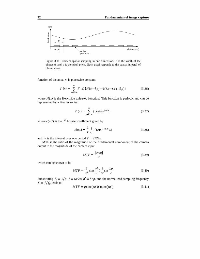
92 Fundamentalsof imagecapture
p
hIll
umin
atio
ndistance (x)
I(x),
activephotosite
Figure3.11: Cameraspatialsamplingin onedimension. h is the width of thephotositeand p is thepixel pitch. Eachpixel respondsto thespatialintegral ofillumination.
functionof distance,x, is piecewiseconstant
I x∞
∑k ∞
I k H x kp H x k 1 p (3.36)
whereH x is theHeavisideunit-stepfunction. This functionis periodicandcanberepresentedby a Fourierseries
I x∞
∑n ∞
c nω ejnωx (3.37)
wherec nω is thenth Fouriercoefficient givenby
c nω1T T
I x e jnωxdx (3.38)
and T is theintegralover oneperiodT 2π ω.MTF is the ratio of the magnitudeof the fundamentalcomponentof the camera
outputto themagnitudeof thecamerainput
MTFc ω
a(3.39)
whichcanbeshown to be
MTF2
ωhsin
wh2
2w
sinωp2
(3.40)
Substitutingfp 1 p, f ω 2π, h h p, andthenormalizedsamplingfrequencyf f fp leadsto
MTF psinc πf h sinc πf (3.41)

3.3Camera and sensortechnologies 93
distance
pixel width
‘Top hat’ profile
Ideal profile
50% overlap
Figure3.12:Somephotositecaptureprofiles.
0 0.05 0.1 0.15 0.2 0.25 0.3 0.35 0.4 0.45 0.50.1
0.2
0.3
0.4
0.5
0.6
0.7
0.8
0.9
1
Normalized spatial frequency f’
MT
F
ideal
top-hat
50% overlap
Figure3.13:MTF for thecaseof idealsampler, h 0, full width sampler, h 1,and50%pixel overlap,h 1 5.
For anidealsampler, thatis, h 0, theMTF is givenby
MTF h 0 psinc πf (3.42)
whichis theexpectedfrequency responsefor asamplerfollowedby azero-orderhold.A samplerthatintegratesover theentirepixel width will have anMTF givenby
MTF h 1 psinc2 πf (3.43)

94 Fundamentalsof imagecapture
For thepixel captureprofilesshown in Figure3.12,thecorrespondingspatialfre-quency responsesaregivenin Figure3.13. Theseindicatesthatcross-talkandfinitepixelwidthcausethespatialfrequency responseto roll off moresharplyathighspatialfrequency. Thevertical linesof metalizationin aninterlinetransfersensorreducetheactivewidth of thephotosite,andshouldimprovetheMTF in thehorizontaldirection.
3.3.3 CCD exposurecontrol and motion blur
In thediscussionsofar it is hasbeenassumedthatthephotositesarebeingcharged,orintegrating,for onewholefield time. High-speedrelativemotionbetweenthecameraandsceneresultsin a blurredimage,sincethe photositesrespondto the integral ofillumination over theexposureperiod. A blurredobjectwill appearelongatedin thedirectionof motion13.
In thecasewhereanobjectmovesmorethanits width duringtheexposureintervaltheilluminationwill bespreadoveragreaternumberof pixelsandeachwill 'see'lesslight. Thatis, astheimageblurs,it elongatesandbecomesdimmer. A machinevisionsystemwhich usesthresholdingto differentiatea bright objectfrom its backgroundcanthus'losesight' of theobject.In avisualservoingsystemthiscanleadto 'rough'motion[65].
A conventionalfilm camerausesamechanicalshutterto exposethefilm for averyshortperiodof time relative to thescenedynamics.Electronicshutteringis achievedon CCDsensorsby discharging thephotositesuntil shortlybeforetheendof field bymeansof the anti-bloomingor integrationcontrol gate. Only the charge integratedover theshortremainingperiod,Te, is transferredto the transportregisters.The ac-cumulatedchargeis reducedproportionally with theexposuretimewhich reducesthesignalto noiseratio of the image.This effect canbecounteredby openingthecam-era's apertureor providing additionalsceneillumination.
The timing of thePulnix camera's integrationperiodhasbeendeterminedexper-imentally by viewing an LED emitting a very short light pulseat a time that is ad-justablerelative to the vertical synchronizationpulse. As shown in Figure3.14 theintegrationperiodalwaysends1msaftertheonsetof verticalblanking.
Considerthe onedimensionalcaseof a moving objectwhosecentroidlocationon the imageplaneis iX t . TheCCD sensorrespondsto the integralof the incidentillumination,sotheperceivedcentroidwill bethemeanover theintegrationperiod
iX1Te
0
Te
iX t dt (3.44)
13It maybepossibleto determinethevelocityof aknown symmetricobjectfrom theshapeof its blurredimage.

3.3Camera and sensortechnologies 95
Activevideo
1ms
2ms4ms
20ms
20ms
8ms
Exposure intervals
Blankinginterval1.6ms
Figure3.14: Experimentallydeterminedexposureinterval of thePulnix camerawith respectto verticalactive timing.
If thetargetis moving ata constantvelocity i X theperceivedcentroidwill be
iX1Te
0
Te
iX 0 i Xt dt (3.45)
iX 0 i XTe
2(3.46)
iX Te 2 (3.47)
whichlagstheactualcentroidby half theexposureinterval. Thusfor afinite exposureinterval, the actualexposuretime shouldbe takenashalfway throughthe exposureperiod.
3.3.4 Linearity
Theluminanceresponseof a CRT monitor
LCRT vγCRT (3.48)
is highly non-linear, wherev is the input signalandγCRT is a valuetypically in therange2.2to 2.8.Thecamerais normallyadjustedfor theinverseresponse
v Lcamγcam (3.49)
whereLcam is the luminanceof the observed sceneand γcam is chosenas 0 45 tocorrectfor the non-linearityof the CRT andrenderan imagewith correctcontrast.Early vacuumtubesensorssuchasiconoscopesin facthadtheappropriatenon-linear

96 Fundamentalsof imagecapture
characteristic.LinearsensorssuchastheorthicontubeandCCDsrequireanon-linearamplifier14.
The transferfunction,or linearity of thecamera's illumination response,is oftenreferredto asgamma, andmany solid statecamerashave a switchto selectγcam 1or 0 45. For machinevisionwork, wheretheimageis not beingdisplayedona CRT,a non-linearcameraresponseservesnousefulpurpose.
3.3.5 Sensitivity
Sensitivity is theDC gainof thesensorto incidentillumination. Factorscontributingto sensitivity include:
Quantumefficiency, ηq, thefractionof incidentphotonsconvertedto electrons.This quantumefficiency is typically around80%but is a functionof thesemi-conductormaterialandwavelengthof thephoton.
Area efficiency or pixel fill factor is the ratio of photositeactive areato totalarea
η fpxpy
pxpy(3.50)
wherepx andpy arethedimensionsof theactive photositesensingarea.Areasof metalizationin eachphotositereducethesensitive area.Frametransfersen-sorshave a higherareaefficiency thaninterline transferdevicessincethereisnometalizedverticaltransportregister.
Charge transferefficiency. Eachtime a packetof charge is moved aboutthesubstrate,somechargecarrierswill belost. Althoughthisfractionis verysmall,charge packetsfrom distantphotositesundergo a greaternumberof transfers.As well asreducingthe apparentintensityof the pixel, the 'lost' charge frombright regionswill be pickedup by subsequentcharge packets,thusreducingcontrastin areasof fine detail. Bright regionsleaving a trail of chargebehindthemresultin streakingof theimage.
Thegainof theon-chipchargeamplifier.
Thegainof outputamplifierwithin thecameraelectronics.
Thegainof theAGC(AutomaticGainControl)stage.
14Transmissionof the non-linearintensity signal hasan advantageousside effect in noisereduction.Signalscorrespondingto low intensityareselectively boostedby thenon-linearityprior to transmissionandthenreducedon display, alsoreducingtheamplitudeof additivenoisein transmission.

3.3Camera and sensortechnologies 97
grey test card
spot meter
CCD cameraunder test
vision system showingintensity histogram
Figure3.15:Experimentalsetupto determinecamerasensitivity.
f -number grey-level sensorluminance(lx)
f/5.6 saturated 2.0f/8 177 0.98
f/11 120 0.52f/16 44.2 0.25
Table3.5: Grey level responseof PulnixTM-6, with 25mmlens,20msexposuretime,no AGC,γ 1, luminance80cd m2.
Sensorsensitivity is typically quotedin unitsof electrons/lux,andmaybe foundin a datasheet.However thesensitivity or overall gainof a completecamerais rarelygivenandmustbedeterminedexperimentally. A suitableexperimentalsetupis shownin Figure3.15wherethethecamerais aimedatauniformly illuminatedgrey testcardanddefocusedsoasto eliminatetheeffect of finetexture.
A spot-readingmeteris usedto determinethe luminanceof thecard,L, andthemeangrey-level of asmallregionin thecenterof theimage,I , is takenasthecamera'sresponse.For a rangeof f -numbersettingsshown in Table3.5 the responseof thePulnixcamerawasdeterminedto be
I11000
F2 12 (3.51)

98 Fundamentalsof imagecapture
0 2 4 6 8 10 12 1480
100
120
140
160
180
Relative illumination
Gre
y le
vel
0 2 4 6 8 10 12 141
2
3
4
5
Relative illumination
Var
ianc
e (g
rey
leve
l^2)
Figure3.16: Measuredresponseof AGC circuit to changingillumination. Topcurveshowsmeangrey-level response.Bottomcurveshowsthegrey-level spatialvariance.
which hasthe form expectedby (3.12) plus a small offset. LuminanceL is mea-suredby thespot-readingmeteras80cd m2 andif theintensitygainof thecameraisKcamgreylevel lx thenfrom (3.12)wemaywrite
11000 Kcamπ804
(3.52)
giving acameragainofKcam 180greylevel lx (3.53)
This is a lumpedgain valuewhich includeslenstransmission,sensorresponse,andcameraanddigitizeranaloggain15. Extrapolatingfrom theexperimentaldata,satura-tion of thedigitizerwill occurwhentheilluminanceat thesensorexceeds1.4lx.
Let usassumethattheminimumdiscernablegrey value(dueto noise)is 5, whichcorrespondsto anilluminanceof 1 4 5 256 27 10 3lux. Usingthefilm speedrelationship(3.18)andanexposureinterval of 40mswe canequatethis sensorto anISOfilm speedof around730.
15DIGIMAX is setto nominal0dB gain,seeSection3.5.2.

3.3Camera and sensortechnologies 99
0 2 4 6 8 10120
140
160
180
200
Time (s)
Gre
y le
vel
0 2 4 6 8 10
140
160
180
200
220
Time (s)
Gre
y le
vel
Figure3.17:Measuredresponseof AGCcircuit to stepilluminationchange.Topcurve is with AGCdisabled,andthebottomwith AGCenabled.
Camerascommonlyhave an automaticgain control (AGC) function which at-temptsto maintainthe 'average'grey-level in the scene. The Pulnix camerahasaquotedAGCgainrangeof 16dB or 2.7stops.Severalexperimentswereconductedtoinvestigatethebehaviour of theAGCcircuit:
1. With constantillumination, imageswerecapturedof a grey card. As increas-ingly largewhitesquareswereaddedto thecardtheintensityof thegrey back-groundareawasreduced.The AGC strategy thusappearsto be maintenanceof the meangrey-level in the sceneeven if this forcesbright sceneareasintosaturation.
2. With constantilluminationandnolensfitted,imageswerecapturedwith avari-etyof neutraldensityfiltersover thecamera.Theresultsplottedin Figure3.16show a plateauin thecameraresponsefor therangeof illuminancelevelsoverwhich theoutputis heldroughlyconstantby theAGC.
At very low illuminancethe gain of the AGC is insufficient to maintainthecameraoutput level. In this regime it can be seenthat the grey-level spatialvariance16 hasincreased,astheamplifierbooststheweaksignalandaccentuates
16Thevarianceof pixel valueswithin a64 64window centeredin theimage.

100 Fundamentalsof imagecapture
thenoisecomponent.
3. Thetemporalresponseof theAGCwasinvestigatedby measuringtheresponseto an averageillumination level which is an offset squarewave. The ratio ofintensitiesis approximately1.5, requiringonly a 3dB gainrangewhich is wellwithin the 16dB rangeof the camera's AGC circuit. The responsewith andwithout AGC is shown in Figure3.17. The former exhibits substantialover-shoottakingaround1s to settle. In a normalsituationa bright objectenteringthescenewouldcauseonly a moderatechangein averageilluminationandthisoscillatoryeffect wouldbelessmarked.An AGC is a non-linearfeedbacksys-tem,andtheresponsewill berelatedto theamplitudeof theinput.
3.3.6 Dark current
In additionto the photo-generatedelectrons,a photositeaccumulatescharge duetodark current. Dark currentresultsfrom randomelectron-holepairsgeneratedther-mally or by tunnelling and is indistinguishablefrom photongeneratedcurrent. Atemperaturerise of 7K will doublethedark current[83]. To minimizeaccumulatedchargedueto darkcurrent,sensorsdesignedfor longexposuretimesarecooled.Shortexposuretimesreducechargedueto bothdarkcurrentandillumination.
Themeandarkcurrentis determinedby dark-referencephotositeswhicharegen-erallycolumnsoneachsideof thearray. Thesearemanufacturedin thenormalmannerbut arecoveredby metalizationsothatonly darkcurrentis accumulated.Thecameraelectronicsusethe signalfrom thesepixelsasa black reference,subtractingit fromtheoutputof theuncoveredpixels.
3.3.7 Noise
A numberof factorscontributeto noisein a CCDsensor:
Photonarrival statisticsresultin photonshotnoise. Photonarrival is a randomprocess[221] andtheprobabilityof detectingaphotonin thetimeinterval t tδt is proportionalto theradiometricintensityEr t (W m2) at time t.
Thephoton-numberstatisticsaregenerallymodelledby a Poissondistributionwith a meanandvariance
nEr
hν(3.54)
σ2n n (3.55)
whereν is thephotonfrequency andh is Planck'sconstant.

3.3Camera and sensortechnologies 101
Photonconversionstatistics,or photoelectronnoise. A photonincidenton asensorof quantumefficiency ηq will produceanelectronwith a probabilityofηq andfail to dosowith a probability1 ηq.
Darkcurrentshotnoise,dueto therandomthermalgenerationof electronscap-turedby thephotosite.
Receiver shotandthermalnoiseintroducedduring amplificationof the accu-mulatedcharge. To minimizethis,a high-gainlow-noiseamplifieris generallyfabricatedon-chipwith theCCDsensor.
Readoutnoisedueto couplingof CCD clockingsignalsinto thesensoroutputsignal.
Patternnoiseor responsenon-uniformity. This is not a true noisesourcebutreflectsavariationin gainbetweenphotosites.Thiseffectarisesfrom variationsin materialcharacteristicsandprocessvariationsin chipmanufacture.Thenon-uniformity is highly dependentoncolorwhichaffectsphotonpenetrationof thematerialandthusthedefectsencountered.
If x is thecameraoutputsignal,thesignalto noiseratio
SNRx2
Σσ2 (3.56)
is a functionof thevariousnoisesourcesjust discussed.The meanandvarianceof grey-level within a smallwindow in the centerof the
imagewerecomputedfor a rangeof illumination levels. To achieve uniform illumi-nationof the sensorthe lenswasremoved andthe illuminancecontrolledby meansof neutraldensityfilters placedin front of the camera.The varianceis plottedasafunction of the meanintensity in Figure3.18. The varianceincreaseslinearly withmeancameraresponseaswouldbeexpectedfor photonshotnoiseby (3.55).Theuseof shortexposuretimesdoesnot appearto have any significanteffect on the outputnoiselevel. Theline correspondsto aSNRof 36dB17.
If the value of eachpixel within the samplewindow is averagedover time thesamplemeanwill approachtheexpectedvaluegivenby (3.54),andthespatialvarianceof the time-averagedpixelswould thenbedueto pixel responsenon-uniformity. Forthe brightestsamplein Figure 3.18 the spatialvariancefalls from 3 5 to 1 0 afteraveraging100frames.
17Thedigitizerquantizationnoisefrom (3.70)is insignificantcomparedto thenoisemeasuredhere.

102 Fundamentalsof imagecapture
50 100 150 2000.5
1
1.5
2
2.5
3
3.5
4
Camera response (grey levels)
Var
ianc
e (g
rey
leve
ls)
Figure3.18: Measuredspatialvarianceof illuminanceas a function of illumi-nance.Pointsmarked'*' aremeasuredwith a 20msexposuretime,and'+' witha2msexposuretime.
3.3.8 Dynamic range
The dynamicrangeof a CCD sensoris the ratio of the largestoutputsignal to thesmallestdiscernibleoutput. The largestsignal, at saturation,is directly relatedtothe capacityof the charge well. At very low illumination levels the responseof thesensoris totally overwhelmedby thedarkcurrentandnoiseeffectsdescribedabove.The smallestdiscernibleoutputis thusthe outputnoiselevel. For a CCD with, forexample,noiseof 100electronsanda chargewell of 100,000electronsthedynamicrangeis 1000or nearly10bits.
3.4 Videostandards
Broadcastandclosed-circuittelevision industriesdominatethemanufactureandcon-sumptionof videoequipment,thusmostcamerasusedfor machinevision work con-form to televisionstandards.Thetwo mostwidely usedstandardsare:
RS170usedin theUSA andJapanwith 525line framesat30framespersecond;

3.4Video standards 103
Active video time
White
Sync
Blankinginterval
0V
−0.3V
backporch sync
pulse5us
frontporch6us
0.7V
time
Blanking/black
line time 64us
Figure3.19:CCIRstandardvideowaveform,1V peakto peak.
CCIR usedin EuropeandAustraliawith 625line framesat 25 framespersec-ond.
Therequirementsof broadcasttelevision arequitedifferentto thosefor machinevi-sion. Broadcasttelevision requireslow transmissionbandwidth,easeof decodingintheviewer's setandminimal humanperceptionof flicker. Interlacing,anartifact in-troducedto addresstheconstraintsof broadcasttelevision is particularlyproblematicfor machinevision andis discussedfurther in Section3.4.1. Thecameraframerate,effectively thesampleratein avisualservo system,is now asignificantlimiting factorgiven the currentand foreseeablecapabilitiesof imageprocessinghardware.Highframerateandnon-interlacedcamerasarebecomingincreasinglyavailablebut areex-pensivedueto low demandandrequirespecializeddigitizationhardware.Introductionis alsohamperedby a lack of suitablestandards.An importantrecentdevelopmentistheAIA standardfor cameraswith digital ratherthananalogoutput,which supportsinterlacedandnon-interlacedimagesof arbitraryresolution.
A television signalis ananalogwaveformwhoseamplituderepresentsthespatialimageintensityI x y sequentiallyasv t wheretime is relatedto thespatialcoordi-natesby therasterizingfunctions
x Rx t (3.57)
y Ry t (3.58)
which aresuchthat the imageis transmittedin a rasterscanpattern.This proceedshorizontallyacrosseachline, left to right, andeachline from top to bottom.Betweeneachline thereis a horizontalblanking interval which is not displayedbut providesa short time interval in which the displayCRT beamcan return to the left sideofscreenprior to displayingthenext line, andcontainsa synchronizationpulse,to keepthe displaypoint in stepwith the transmittedwaveform. The video waveform for

104 Fundamentalsof imagecapture
1
57
3
Odd field
2468
Even field
Figure3.20: CCIR format interlacedvideo fields. Note the half line at top andbottomwhichdistinguishesthetwo field types.
oneline time is shown in Figure3.19,anddetailsof timing aregiven in Table3.6.Typically video signalsare1V peak-to-peak.The averagevalueof the luminancesignalis referredto asthepedestalvoltage.Theback-porch periodis usedto providea referenceblankinglevel for the intensitywaveform. For RS170video the voltagecorrespondingto blackis raisedslightly, 54mV, abovetheblankinglevelby theblack-setupvoltage.
An interlacedvideo signalcomprisespairsof sequentialhalf-vertical-resolutionfields, displacedvertically by oneline, asshown in Figure3.20. All even lines aretransmittedsequentiallyin onefield, followedby all oddlinesin thenext field. Thisartifice allows a screenupdaterate of 50Hz which is above the flicker perceptionthresholdof humanviewers. A field is not an integral numberof line times— forCCIR standardvideo thereare287.5linesperfield. Even fieldsbegins with a half-line, andodd fieldsendwith a half-line asshown in Figure3.20. A CCIR frameisdefinedascomprisinganevenfield followedby anoddfield. Betweeneachfield thereis averticalblankinginterval, whichalsoservesfor beamretraceandsynchronization.Detailsof verticalwaveformtiming aregivenin Table3.7.
A compositecolor signalcomprisesthe luminancesignalalreadydescribedwitha superimposedsuppressed-carrierchrominancesignal. The chrominancesignal isphasemodulatedto encodethe two color componentsignals. To demodulatethissignalthecarriersignal18 mustbe reinsertedlocally. A few cyclesof thecarrierfre-quency, thecolor burst, aretransmittedduringthebackporchtime to synchronizethe
18ForCCIR thecolorsubcarrierfrequencyis approximately4.34MHz.

3.4Video standards 105
Period Fraction Time(µs)
Total line (H) 1H 64.0H blanking 0.16H 12.0 0.25H syncpulse 0.08H 4.7 0.2
Table3.6: Detailsof CCIRhorizontaltiming.
Period Fraction Time
Total field (V) 1V 20ms312.5H
Total frame 2V 40ms625H
Active frametime 575HActive field time 287.5HV blanking 25H 1.6ms
0.08V
Table3.7: Detailsof CCIRverticaltiming.
localcolorsubcarrieroscillator. Thismethodof encodingcoloris chosensoasto min-imize interferencewith the luminancesignalandto provide backwardcompatibility,that is, allowing monochromemonitorsto satisfactorilydisplaya color videosignal.Bright fully-saturatedregionscausetheCCIRcolor videosignalto peakat 1.23V.
3.4.1 Interlacing and machinevision
As alreadydescribeda framein aninterlacedimagecomprisestwo videofields. Be-fore the framecanbeprocessedin a machinevision systembothfieldsmustbereadinto a framestoreto recreatetheframe.This processis referredto asdeinterlacing.
Ordinarilydeinterlacingdoesnot causeany problem,but whenimaginga rapidlymoving objectthe time at which the field imagesarecaptured,or the type of shut-teringused,is critical. A frameshutteredcameraexposesbothfieldssimultaneously,whereasafieldshutteredcameraexposeseachfield prior to readout.Frameshutteringis feasiblewith a frametransferCCD sensor. The Pulnix camerausedin this workemploysaninterlinetransferCCDsensorandis capableonly of field shuttering.Fig-ure3.21shows theeffect of deinterlacingan imageof a rapidly moving objectfroma field shutteredcamera.For moderatevelocity the objectbecomesraggedaroundthe edges,but for high velocity it appearsto disintegrateinto a cloud of short linesegments.Oneapproachto circumventingthisproblemis to treatthefieldsasframesin their own right, albeitwith half theverticalresolution.This hastheadvantagesofproviding twicethevisualsamplerate,while eliminatingdeinterlacingwhichrequires

106 Fundamentalsof imagecapture
Figure3.21:Theeffectsof field-shutteringon anobjectwith moderate(top) andhigh (bottom)horizontalvelocity.
additionalhardwareandincreaseslatency.Whenusingvideofieldsin thismannerit shouldberememberedthatthephotosites
for thetwo fieldsareoffsetverticallyby oneline in thesensorarray, andthusoddandevenfield pixelscorrespondto verticallydisparatepointsin thescene19. This resultsin theverticalcoordinatesbeingsuperimposedwith a 25Hz squarewave with 1pixelpeak-to-peakamplitude.Althoughtheimageplanedisplacementis small,theapparentvelocity is very high,around12pixel s, andmaycauseproblemswith targetvelocityestimators.To berigorouswhenusingfield ratedatathiseffectshouldbecorrectedfor(differentcameracalibrationsmadefor eachfield) but in practicethis is rarelydone.
3.5 Imagedigitization
The digital imagesusedin machinevision area spatiallysampledrepresentationofthecontinuousimagefunctionI x y . Thefirst stepin machinevisionprocessingis todigitize theanalogvideowaveformwhich representstheimagefunction. Thewave-form is sampledandquantizedandthe valuesstoredin a two-dimensionalmemoryarrayknown as a framestore. Thesesamplesarereferredto aspictureelementsor
19Somecamerasareableto providean interlacedoutputthatusesonly a singlefield from the sensor.Thatis, theyoutputevenfield, evenfield, evenfield . . .

3.5Imagedigitization 107
pixels, andtheir magnitudeis often referredto asgrey-level or grey value. Eachrowof datain theframestorecorrespondsto oneline timeof theanalogvideosignal.
This sectionwill examinethe variousprocessingstagesinvolved in imagedig-itization, both in generaltermsand also with particular referenceto the DatacubeDIGIMAX [73] hardwareusedin thiswork.
3.5.1 Offset and DC restoration
TheanalogwaveformfromthecameramayaccumulateDC offsetduringtransmissionandamplification. DC restorationis the processof eliminatingtheseoffsetswhichwould otherwisebe manifestas brightnessoffsets, introducingerrorsin perceivedimagecontrast. The waveform is sampledduring the back porchperiod, and thisvalue(maintainedby a sampleandhold network)is subtractedfrom thevideosignalfor the next line so as to restorethe DC level. Ideally the signal's black referencevoltageis relatedto theoutputof thedarkreferencephotositeswithin thecamera.
The DIGIMAX digitizer allows anoffset to be specified,so that the signallevelcorrespondingto blackcanbeset to correspondwith a grey valueof 0. The PulnixTM-6 camerahasbeenobservedto outputa blacklevel 25mV above blankinglevel,despiteits claimedCCIRoutputformat.
3.5.2 Signalconditioning
Prior to digitizationtheanalogsignalfrom thecameramustbefilteredto reducealias-ing andpossiblyto screenout thechrominancesignalfrom acompositevideosource.The DIGIMAX hasa 6th orderfilter with settablebreakfrequency. For a 512pixelsensora breakfrequency of 4.5MHz is usedwith a 40dB octave rolloff. Howeversucha filter will have a substantialeffect on frequency componentswithin the passbandwhich will bemanifestedin reducedcontrastandblurring of fine imagedetail,compoundingtheeffectdueto thecamera's MTF. More importantlythesignalwill bedelayeddueto thephasecharacteristic,seeFigure3.22,of theanti-aliasingfilter. Thismustbeconsideredin thecameracalibrationprocesssinceit shifts the entireimagehorizontallyasshown by thestepresponseFigure3.23.
Thesignalconditioningstagemayalsointroduceagain,Kdig, prior to digitizationto improve thesignalto noiseratio for darkscenes.TheDIGIMAX digitizer allowsgainsettingsin therange-4dB to +10dB in 2dB steps,whichcorrespondsto +1.3to-3.3stopsat thecamera.
3.5.3 Samplingand aspectratio
At thesamplerthepiecewiseconstantoutputsignalcorrespondingto thecamerapho-tositeshasbeendegradedand'roundedoff ' dueto the limited bandwidthelectronics

108 Fundamentalsof imagecapture
-1.8
-1.7
-1.6
-1.5
-1.4
-1.3
-1.2
0 1 2 3 4 5 6 7 8 9 10
x106
Pha
se d
elay
(pi
xels
)
Frequency (Hz)
Group delay of 6th order Butterworth 4.5MHz
Figure3.22:Phasedelayof 6thorder, 4.5MHz Butterworthlow-passfilter show-ing delay in pixels as a function of frequency of the video signal. For videodigitizationtheNyquistfrequency is 5MHz.
0
0.2
0.4
0.6
0.8
1
1.2
0 1 2 3 4 5 6 7
Step response 6th order Butterworth 4.5MHz
Time (pixels)
Res
pons
e
Figure3.23:Simulatedstepresponseof 6thorder, 4.5MHzButterworthlow-passfilter.

3.5Imagedigitization 109
512 active pixels
616 pixels per line
64.36us line time
52.5us active video (752 pixels)
10.25us
Video
sync
DIGIMAXactivevideo
blank
87 pixels
Figure3.24:Measuredcameraanddigitizerhorizontaltiming.
andtransmission.This signalmustbesampledto generatethe framestorepixel val-uesI f i j wherei and j areframestorerow andcolumnaddresses.Importantly, theframestorepixels, I f , arenot necessarilymappedexactly ontocamerapixels. In or-der to correctlysamplethe camerasignal andaddressthe framestorethe camera'srasterizingfunctions(3.57) and (3.58) mustbe replicatedwithin the digitizer. Thesynchronizationinformationwithin thevideosignalis usedfor this purpose.
A digitizer samplesthe video signal v t at a frequency fd, which is generallyan integral multiple of the horizontalsynchronizationpulsefrequency, fh. For theDIGIMAX digitizer [75]
fd 616fh (3.59)
Suchsamplingdoesnot necessarilyalign the sampleswith the output of spatiallyadjacentphotosites.Typical digitizerssamplethe incomingvideo into an array of512 512samples20, soeachline has512samplesirrespectiveof thenumberof pho-tositesper line in the sensor. Eachdigitized pixel is thereforenot an independentpoint sampleof the incident illumination, an effect which hasseriousramificationsfor many machinevisionalgorithms,particularlyedgedetectors,whichmakeassump-tionsaboutindependentpixels[15]. Thispixel re-samplingfurtherreducestheMTF,andalsoalterstheaspectratio of thestoredimage.
Figure 3.24 shows the timing waveformsmeasuredfor the Pulnix cameraandDIGIMAX. The active video time of the camerais the responseof the unmasked
20SinceCCIRvideohas575active linesperframe,seeTable3.7,thelowest63 linesof theframe(11%)arelost. Moremoderndigitizersandframestoresallow captureof anentireCCIR frame.

110 Fundamentalsof imagecapture
Parameter Value
Sensorwidth 6.5 mmSensorheight 4.8 mmHorizontalactive pixels 752 pixelsVerticalactive lines 582 pixelsPixel width (px) 8.6 µmPixel height(py) 8.3 µm
Table3.8: Manufacturer'sspecificationsfor thePulnixTM-6 camera.
pixelsandis readilymeasuredwith anoscilloscopefrom thevideowaveformwith thesensorilluminatedandno lensfitted21. Theactive videoregion of theDIGIMAX is512 pixels long beginning 87 pixelsafter the horizontalsynchronizationpulse[75].Clearly the active video timesof the cameraanddigitizer do not overlapcorrectly.As a consequencethedigitizedimagecontainsa blackstripe,approximately10 pix-elswide, on the left handedgeof the imageandthe samenumberof pixelsarelostfrom theright handedge.TheDIGIMAX' stiming is appropriatefor RS170wherethehorizontalblankingperiodsareshorterthanfor CCIR.
The camera's 752 camerapixelsper line, from Table3.8, arere-sampledat 512points,andthis ratio canalsobeexpressedin termsof thedigitizerandcamerapixelfrequencies
βfcfd
752512
1 47 (3.60)
Eachframestorepixel thuscontainsinformationfrom nearly1.5cameraphotosites.Theparameterβ is importantfor many of thecameracalibrationtechniquesdis-
cussedin Section4.2.2,anda numberof techniqueshave beenproposedfor its deter-minationsinceit is highly dependentuponthecameraanddigitizer used.Tsai [169]suggestsobservinginterferencepatternsin thedigitized imagedueto beatingof thecamera's pixel clockwith thedigitizer, but nosuchpatternis discerniblewith thisPul-nix camera.Penna[205] describesanapproachbasedon imaginganaccuratesphere,andfitting a polynomialcurve to thecapturedimage.
An experimentto accuratelydetermineβ wasconductedusingthefrequency ratiomeasurementcapabilityof anHP5115AUniversalCounter. Thecamerapixel clockandthehorizontalsynchronizationpulsesignalsarebothavailableandtheir ratiowasmeasuredas
fcfh
9043 (3.61)
21Themeasuredline timeat64.36µsis slightly longerthantheCCIRstandard64µs.

3.5Imagedigitization 111
Parameter Value
αx 79.2 pixel/mmαy 120.5 pixel/mm(framemode)αy 60.2 pixel/mm(field mode)
Table3.9: Derivedpixel scalefactorsfor thePulnixTM-6 cameraandDIGIMAX digitizer.
andknowledgeof DIGIMAX operation,(3.59),leadsto
βfcfd
fcfh
fhfd
1 468 (3.62)
Framestorepixel aspectratio is a function of the camera's pixel dimensionsandthesamplingratioβ. Thedimensions22 of thephotosites,px py, for thecamerausedin this work aregivenin Table3.8.23 Thescalefactorsαx andαy arereadilyderivedfrom thephotositedimensions
αx1
β pxpixel m (3.63)
αy1py
pixel m (3.64)
An imageon thesensorwith dimensionsof W H will appearin the framestorewith dimensions,in pixels,of αxW αyH. In generaltheaspectratio, height/width,will bechangedby αy αx, andthis hasbeenverifiedexperimentallyas1 52. Whenprocessingvideofields ratherthanframes,adjacentrows in the imageareseparatedby two rowson thesensor. Theverticalscalefactorbecomes
αy1
2pypixel m (3.65)
andtheratioαy αx is now 0 761.Thesescalefactorsaresummarizedin Table3.9.Thetiming relationshipsjustdescribed,whichareafunctionof theparticularcam-
eraanddigitizer used,directly affect horizontaldisplacementof the imageanddig-itized imageaspectratio. Both of thesefactorswill affect the intrinsic parametersof the camera,andaresignificantin cameracalibrationwhich will be discussedinSection4.2.
Figure3.25shows thecoordinatesystemsthatwill beusedthroughoutthis work.Thedirectionof pixel scanningwithin theCCDsensoreliminatestheimageinversionpresentin theearlierlensequations(3.30)and(3.31). Theworld X andY directions
22Manufacturer'sspecificationsdonot discusstoleranceon pixel dimensions.23Generallythepixelscellsarenot squarethoughcameraswith squarepixelsareavailable.

112 Fundamentalsof imagecapture
Z
X
Y
Xi
Image plane
Yi
X0 Y0,( )+
Figure3.25:Cameraandimageplanecoordinatesystems.
correspondto theimageplaneiX andiY directionsrespectively. Thoseequationscannow bewritten in termsof pixel coordinatesas
iXαx f xz f
X0 (3.66)
iYαy f yz f
Y0 (3.67)
(3.68)
where X0 Y0 is thepixel coordinateof theprincipalaxisdefinedearlier.
3.5.4 Quantization
The final stepin the digitizationprocessis to quantizethe conditionedandsampledanalogsignalby meansof a high-speedanalogto digital converter. The sampleisquantizedinto ann-bit integerwith valuesin therange0 to 2n 1. Typically theblackreferencewould correspondto 0 andthe peakwhite level to 2n 1. The quantizedsignal,xq t , canbewritten in termsof theoriginal signal, x t , as
xq t x t eq t (3.69)
whereeq t is thequantizationnoisewhich is assumedto have a uniform distributionover therange 1
212 andameansquaregivenby
e2 112
(3.70)
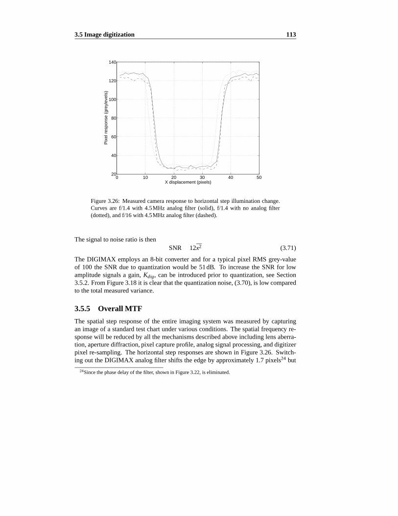
3.5Imagedigitization 113
0 10 20 30 40 5020
40
60
80
100
120
140
X displacement (pixels)
Pix
el r
espo
nse
(gre
ylev
els)
Figure3.26: Measuredcameraresponseto horizontalstepillumination change.Curves are f/1.4 with 4.5MHz analogfilter (solid), f/1.4 with no analogfilter(dotted),andf/16 with 4.5MHz analogfilter (dashed).
Thesignalto noiseratio is thenSNR 12x2 (3.71)
The DIGIMAX employsan 8-bit converterandfor a typical pixel RMS grey-valueof 100 the SNR dueto quantizationwould be 51dB. To increasethe SNR for lowamplitudesignalsa gain, Kdig, canbe introducedprior to quantization,seeSection3.5.2.FromFigure3.18it is clearthatthequantizationnoise,(3.70),is low comparedto thetotalmeasuredvariance.
3.5.5 Overall MTF
The spatialstepresponseof the entire imagingsystemwasmeasuredby capturinganimageof a standardtestchartundervariousconditions.Thespatialfrequency re-sponsewill bereducedby all themechanismsdescribedabove includinglensaberra-tion, aperturediffraction,pixel captureprofile,analogsignalprocessing,anddigitizerpixel re-sampling.Thehorizontalstepresponsesareshown in Figure3.26. Switch-ing out theDIGIMAX analogfilter shifts theedgeby approximately1.7pixels24 but
24Sincethephasedelayof thefilter, shown in Figure3.22,is eliminated.
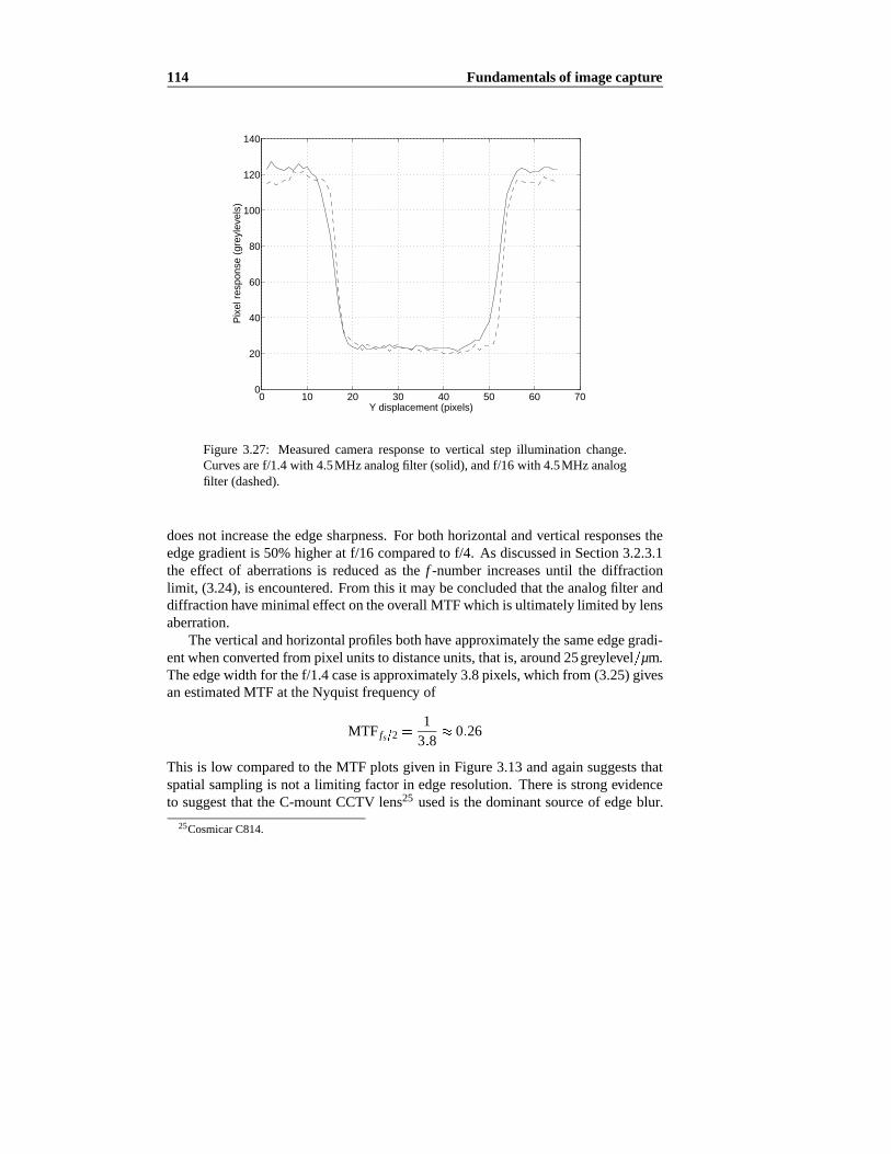
114 Fundamentalsof imagecapture
0 10 20 30 40 50 60 700
20
40
60
80
100
120
140
Y displacement (pixels)
Pix
el r
espo
nse
(gre
ylev
els)
Figure 3.27: Measuredcameraresponseto vertical step illumination change.Curvesaref/1.4 with 4.5MHz analogfilter (solid),andf/16 with 4.5MHz analogfilter (dashed).
doesnot increasetheedgesharpness.For bothhorizontalandvertical responsestheedgegradientis 50%higherat f/16 comparedto f/4. As discussedin Section3.2.3.1the effect of aberrationsis reducedas the f -numberincreasesuntil the diffractionlimit, (3.24),is encountered.Fromthis it maybeconcludedthattheanalogfilter anddiffractionhaveminimaleffectontheoverallMTF whichis ultimatelylimited by lensaberration.
Theverticalandhorizontalprofilesbothhave approximatelythesameedgegradi-entwhenconvertedfrom pixel unitsto distanceunits,thatis,around25greylevel µm.Theedgewidth for thef/1.4 caseis approximately3.8pixels,whichfrom (3.25)givesanestimatedMTF at theNyquistfrequency of
MTF fs 21
3 80 26
This is low comparedto theMTF plots givenin Figure3.13andagainsuggeststhatspatialsamplingis not a limiting factor in edgeresolution.Thereis strongevidenceto suggestthat the C-mountCCTV lens25 usedis thedominantsourceof edgeblur.
25CosmicarC814.

3.5Imagedigitization 115
low−passfilter ZOH
sampler
Figure3.28: Typical arrangementof anti-aliasing(low-pass)filter, samplerandzero-orderhold.
Theselensesaremassproducedcommodityitemsfor applicationssuchassurveillanceandarelikely to bedesignedfor low unit costratherthanimagequality. It hasbeensuggested[52] thattheformatof C-mountlenses,particularlythelongback-focaldis-tanceseverelyconstrainstheopticaldesign.C-mountlensesarehowever commonlyusedwithin themachinevisionandroboticsresearchcommunity.
3.5.6 Visual temporal sampling
In a visual servo systemthe cameraperformsthe function of the sampler. An idealvisualsamplerwould capturetheinstantaneousstateof thesceneandin practicethiscanbeapproximatedby choiceof a suitablyshortexposureinterval. Digital controlsystems,asshown in Figure3.28, typically includean analogprefilter betweenthesensorandthe digitizer asananti-aliasingdevice. Suchfilters arelow-passandde-signedto attenuatesignalsabove the Nyquist frequency so that, whenaliasedintolower frequenciesby thesampler, they will not bedetrimentalto the control-systemperformance[95].
The effect of aliasingdue to camerasamplingresultsin the well known effectwhere,in movies, the wheelson wagonscanappearto rotatebackward.In a visualservo systemit is difficult to conceptualizeananalogprefilter— this wouldbesomeoptical device that transmittedlow-frequency sceneintensitychangebut attenuatedhigh-frequency change.Intuitively it canbe seenthat suchan effect is achieved bymotionblur. A pointoscillatingathighfrequency in thescenewill appear, with a longexposureinterval, to bea blur andhave little if any apparentmotion. While rapidlyoscillatingtargetsareunlikely to beencountered,cameraoscillationdueto manipula-tor structuralresonanceis a significantissueandis discussedfurtherin Section8.1.4,whereit is shown that resonancesexist at frequenciesconsiderablygreaterthanthevisualNyquistfrequency.
Simulationsof cameraresponseto sinusoidaltargetmotionshow themagnitudeofthemotiondetectedby thecamerais a complex functionof targetmotionmagnitudeand frequency as well as cameraexposureinterval and threshold. The simulationmodelstheindividualphotositechargeintegrationasthetargetintensityprofilemoveswith respectto thephotositearray. Theintegrationis performedusinga largenumberof time stepswithin eachchargeintegrationinterval. Thedominantcharacteristicfor

116 Fundamentalsof imagecapture
sinusoidaltarget motion up to the Nyquist frequency is a linearphasecharacteristicdueto thelatency associatedwith theexposureinterval givenpreviouslyby (3.47).
AbovetheNyquistfrequency it is notpossibleto examinethemagnitudeandphaseof sinusoidalcomponentssince,dueto frequency folding, the input andoutputfre-quency arenot equal. The approachusedin simulationis to assumetarget motionwith a uniform spectrumabove the visualNyquist frequency andexaminethe RMSmagnitudeof the simulatedcameraoutputwhich representsnoiseinjectedinto thecontrollerby super-Nyquisttargetmotion.Thetargetmotion
x t H r t βt (3.72)
is generatedby high-passfiltering a vector of randomnumbers,r t . In this casethe filter selected,H , is a 6th orderType I Chebyshev filter with a breakfrequencyof 30Hz and 3dB passbandripple. For small amplitudetarget motion the cameraoutput is highly dependenton wherethe target imagelies with respectto the pixelboundaries.To counterthisthehighfrequency targetmotionis addedto arampsignal,βt, whichslowly movesthetargetcentroidby 1pixelover thesimulationintervalof 64field times.This rampis removedbeforecomputingtheRMS valueof thesimulatedcameraoutput. Figure3.29shows the magnituderesponseof the camerasimulatedin this mannerfor two differentexposureintervals. It can be seenthat the cameraattenuatesthis super-Nyquistsignalandthat theattenuationincreaseswith exposureinterval. Intuitively this is reasonablesinceimageblur will increasewith exposureinterval. Figure3.30shows, for a constantexposureinterval, theeffect of varyingthethreshold.The cameraresponseis greatestfor a normalizedthresholdof 0.5 whichis the midpoint betweenbackgroundandforegroundintensity. Greatestattenuationof super-Nyquist componentscanbe achieved by usinga low thresholdanda longexposureinterval.
3.6 Cameraand lighting constraints
This sectionsummarizesthe issuesinvolved in the selectionof camerasettingsandsceneillumination. Therequirementsfor visualservoing are:
a largedepthof field soasto avoid imagefocusproblemsasthecameramovesdepthwisewith respectto thescene;
shortexposureinterval to reducemotion blur andhave thecameracloselyap-proximateanidealvisualsampler;
theobjectbeof sufficient sizeandbrightnessin theimagethatit canberecog-nized.

3.6Camera and lighting constraints 117
0 1 2 3 4 5 6 70
0.5
1
1.5
2
2.5
3
3.5
4
Target RMS (pixels)
Cam
era
outp
ut R
MS
(pi
xels
)
Figure3.29: Magnituderesponseof simulatedcameraoutputversustarget mo-tion magnitudefor variousexposureintervals: 2ms (*), 20ms(+). Dottedlinecorrespondsto unit gain.Thresholdis 0.5.
0.1 0.2 0.3 0.4 0.5 0.6 0.7 0.8 0.90
0.05
0.1
0.15
0.2
0.25
0.3
0.35
0.4
0.45
0.5
Threshold (normalized)
RM
S o
uput
/inpu
t
Figure3.30:Magnituderesponseof simulatedcameraoutputto changingthresh-old for constanttargetmotionmagnitude.Exposureinterval is 2ms.

118 Fundamentalsof imagecapture
Quantity Lower bound Upperbound
focal magnification(3.8) field of view (3.10),(3.11)lengthf geometricdistortionf -number depthof field (3.19),(3.20) diffraction(3.24)F imagebrightness(3.12)
SNR(3.56)exposure imagebrightness(3.12) imageblurinterval Te SNR(3.56)illuminanceEi imagebrightness(3.12) subjectheating
SNR(3.56)
Table3.10:Constraintsin imageformation.Therelevantequationsarecited.
Theserequirementsareconflicting— for instancedepth-of-fieldrequiresasmallaper-turewhichcombinedwith theneedfor shortexposuretimegreatlyreducestheimageintensity. Table 3.10 lists the parametersand indicatesthe factorsthat control theupperandlowerboundsof acceptablesettings.
A spreadsheet,seeFigure3.31,is a convenientway to appreciatetheinteractionsof theseparameters.Thetopsectioncontainsparametersof thelensanddigitizer, andthesecorrespondto the8mmlensusedin thiswork.26 Thenext sectioncomputesthediffractionblur by (3.24),andthehyperfocaldistancefor thespecifieddiametercircleof confusionby (3.21).Thenearandfar focusboundscomputedby (3.19)and(3.20)arealsoshown. For this casea reasonabledepthof field canbeobtainedat f/5.6 withthefocuspointsetto 700mm. Thediffractioneffect is negligible at only 0.3pixels.
The lowestsectionof thespreadsheetcomputesfield of view, objectimageplanesizeat two settabledistancesfrom thecamera;nearandfar. Incidentlightmeterread-ings andestimatedcameragrey-level responsearecalculatedbasedon the distancebetweenobjectandlight source.In this examplethe lighting systemcomprisestwo800W studiospot-lightssituated3m behindthe camera.Given the shortexposuretime andsmallaperturesettinga significantamountof illumination is requiredto ob-tain a reasonablecameraresponseat thefar objectposition.
3.6.1 Illumination
An 800W photographicfloodlampwith a quartzhalogenbulb hasa luminouseffi-ciency of 20lm W. Assumingthe emittedlight is spreadover πsr27 the luminousintensityis
800 20π
5100cd
26Lenstransmissionof 80%is anestimateonly.27Onequarterspheresolidangle.

3.6Camera and lighting constraints 119
Camera and lens settingsAperture (F) 5.6Focal length (f) 8 mmLens tranmission 80 %Exposure time (Te) 2 msPixel scale (αx) 80 pixel/mmPixel scale (αy) 60 pixel/mmFocus setting 700 mmHyperfocal distance 922 mmDiffraction 3.79 µm = 0.30 pixels
Circle confusion diam 1 pixelDepth of field 425 mm, to INF mm
Object apparent sizeNear Far
Object range: 600 3000 mmObject diameter (d) 50 mm = 54.1 10.7 pixelMagnification 0.014 0.003Framestore pixel scale factor (X) 1.08 0.21 pixel/mmFramestore pixel scale factor (Y) 0.81 0.16 pixel/mmFIeld of view: width 474 2394 mm
height 631 3191 mm
Illumination and object brighnessLight position -3000 mm 10186 10186 cdLight power 1600 W 786 283 lxLuminous efficiency 20 lm/W 393 141 ntSphere fraction 0.25 11.47 9.99 EVSurface reflectance 0.5 1.26 0.45 lx
220 79 grey-levels
Figure3.31:Spreadsheetprogramfor cameraandlighting setup.Input variablesarein grey boxes. Imageplaneobjectsizeandfield of view arecalculatedfortwo cameradistances;nearandfar. Objectbrightness,in lightmeterunits andestimatedcameragrey-level, is computedbasedon thedistancebetweenobjectandlight source.

120 Fundamentalsof imagecapture
0.1 0.2 0.3 0.4 0.5 0.6 0.7 0.8 0.9 110
2
103
104
105
Distance from camera (m)
Illum
inan
ce (
lx)
Figure3.32: Comparisonof illuminancedueto a conventional800W floodlamp(dashed)and10 cameramountedLEDs(solid)asa functionof distancefrom thecamera.It is assumedthat theLEDs are15cd eachandmountedat thecamera,andthefloodlampis 3m behindthecameraandradiatinglight over πsr.
If thelampis positioned3m away from theobjecttheilluminancewill be
510032 570lx
Recentlyhigh-intensitylight emitting diodes(LEDs) have becomeavailable. Atypical device hasan intensityof 3cd at 20mA with a 7 beamwidth. At the peakcurrentof 100mA theintensitywould be15cd, andif theLED weremountedon thecameraandthe objectdistancewas0.5m the illuminancewould be 60lx. Thustencamera-mountedhigh-powerLEDsexceedtheilluminanceof averyhot800W studiofloodlampsituatedsomedistanceaway. A comparisonof theeffective illuminanceoffloodlampandLEDs for varyingobjectdistanceis givenin Figure3.32showing thatthe LEDs arecompetitive for target illumination up to 600mm. Thesecalculationshavebeenbasedonphotometricunits,thoughasshown in Figure3.4,atungstenlampanda redLED at 670nm emit mostof their radiationin a spectralregion wherethesensitivity of a CCDsensorgreatlyexceedsthatof theeye.
In thevisualservoing applicationthecamera's electronicshutteris openfor only

3.7The human eye 121
10%of the time28 so 90%of thesceneillumination is essentiallywasted.TheLEDschemecanbefurtherrefinedby pulsingtheLED sothatit is lit only while thecam-era's electronicshutteris 'open'. At a 10%duty-cycle theLED peakcurrentcansub-stantiallyexceedthecontinuousratingandexperimentshaveshown thatpeakcurrentsof 400mA arepossible.However thelight outputdoesnot increaseproportionallytocurrentandthis is discussedfurtherin AppendixE.
A pulsedLED light sourcehasbeenbuilt with a ring of 10 high-intensityLEDsplacedaroundthecameralens,seeFigureE.1. A controlbox,describedin AppendixE, allowsthecurrentpulseheight,width andstartingtime to beadjusted.Theadvan-tagesof this light sourcearethatit is lightweight,rugged,haslow heatoutput,andlikea miner's cap-lampdirectslight on thesubjectof interest.Its principaldisadvantageis that the light outputis unevendueto theway in which thepoolsof light from theindividualLEDsoverlap.
3.7 The human eye
The humaneye hasmany importantdifferenceswhencomparedto a CCD sensor.The eye is approximatelysphericalwith a diameterof 15mm andlight is sensedbyphotoreceptorslocatedin the retinaat the backof the eye. In normaldaylight con-ditions conephotoreceptorsareactive andthesearecolor sensitive: 65% sensered,33%sensegreenandonly 2% senseblue. The conesareapproximately3µm in di-ameterand34,000of themarepackedinto thefovealareaof theretinawhich is only0.6mmin diameter. Thephotoreceptordensityin therestof theretinais considerablylower. Theeye hashigh resolutiononly over thefovealfield of view of a few degreesbut subconsciouseye motiondirectsthe foveaover theentirefield of view. Thedis-tancebetweenthelensandretinais approximatelyconstantat 15mmsofocussingisachievedby muscleswhichchangetheshapeof thelens.
Conephotoreceptorshave a dynamicrangeof 600andthepupil, equivalentto theiris of a lens,variesin diameterfrom 2 to 8mmwhichprovidesfor a factorof 16 (10in older people)in dynamicrange. At very low light levels the rod photoreceptorsbecomeactive andprovide anotherfactor of 20 in dynamicrange. The rod sensorsaremonochromaticand their density in the fovea is only 7% of that of the cones,but increasesin the peripheralregion. Rod sensitivity is chemicallyadaptedwitha time constantof tensof minutes. The overall dynamicrangeof the eye is thusapproximately100,000.
Theeye hasthreedegreesof rotationalmotion. Themusclesthatactuatethehu-maneyearethefastestactingin thebodyallowing theeye to rotateatupto 600deg sand35,000deg s2 for saccadicmotion [270]. Smoothpursuiteye motions,involvedin trackingamovingobject,operateatupto 100deg s[214]. Rotationabouttheview-
28A 2msexposurefor every20msvideofield.

122 Fundamentalsof imagecapture
ing axis,cyclotorsion,is limited andthemaximum,rangingfrom 5 to 20deg, variesbetweenindividuals.

Chapter 4
Machine vision
Computervision is the applicationof a computersystemfor receiving andprocess-ing visual information. It comprisestwo broadareas:imageprocessingandimageinterpretation.The latter, often referredto asmachine vision, is typically appliedtopart inspectionandquality control,andinvolvestheextractionof a small numberofgenerallynumericfeaturesfrom theimage.Theformeris theenhancementof imagessuchthat the resultingimagemoreclearlydepictssomedesiredcharacteristicsfor ahumanobserver, andis commonlyappliedto medicalandremotesensingimagery.
Section4.1 introducesthe conventionalcomputervision topicsof segmentationandfeatureextraction. Particularemphasisis given to binary imageprocessingandmomentfeaturessincetheseprovide a cost-effective andtractablesolutionto video-rateimagefeatureextraction.It is importantto notethatvisualservo techniquesbasedonbinaryimagefeaturesareequallyapplicableto moreelaboratelyobtainedfeatures,providedthattheprocessingrateis highandthelatency is low.
Section4.2discussestheimportanttopicsof close-rangephotogrammetry, cameracalibrationandeye-handcalibration.Theseareimportantin understandingprior workintroducedin thenext chapter, andalsoto completethecharacterizationof thecameraanddigitizerusedin this work.
4.1 Imagefeatureextraction
Imageinterpretation,or sceneunderstanding,is the problemof describingphysicalobjectsin a scenegiven an image,or images,of that scene. This descriptionis intermsof, generallynumeric,imagefeatures.
Theprincipalrole of imagefeatureextractionis to reducethecameraoutputdatarate to somethingmanageableby a conventionalcomputer, that is, extracting the'essence'of thescene.An imagefeature is definedgenerallyasany measurablere-
123

124 Machine vision
lationshipin animage. Jang[135] providesa formal definitionof featuresasimagefunctionals
fImage
F x y I x y dxdy (4.1)
whereI x y is the pixel intensityat location x y . The functionF is a linear ornon-linearmappingdependingon the feature,andmay alsoincludedeltafunctions.Somespecificexamplesof imagefeaturesinclude:
the p q th ordermoments
mpqImage
xpyqI x y dxdy; (4.2)
For a binaryimagem00 is theobjectarea,and m10 m01 is thecentroid.Mo-mentfeatures,discussedfurtherin Section4.1.2,arewidelyusedin visualservosystems[17,65,88,92,116,212] dueto thesimplicity of computation;
templatematchingby cross-correlationor sumof squareddifferences[198] todeterminethe coordinateof somedistinctive pixel patternin the image. Thepatternmaybeanedge,corneror somesurfacemarking;
lengths,or orientation,of theedgesof objects;
lengths,or orientation,of line segmentsconnectingdistinctobjectsin thescenesuchasholesor corners[104,198,236]. Feddema[91,92] usedlinesbetweenthecentroidsof holesin a gasketto determinethegasket'spose.
Two broadapproachesto imagefeatureextractionhave beenusedfor visualservoingapplications;whole scenesegmentation,and featuretracking,andaredescribedinsections4.1.1and4.1.4respectively.
4.1.1 Whole scenesegmentation
Segmentationis theprocessof dividing animageinto meaningfulsegments,generallyhomogeneouswith respectto somecharacteristic.Theproblemof robustly segment-ing a sceneis of key importancein computervision,andmuchhasbeenwrittenaboutthe topic and many methodshave beendescribedin the literature. Haralick [106]providesa survey of techniquesapplicableto static imagesbut unfortunatelymanyof thealgorithmsareiterativeandtime-consumingandthusnotsuitablefor real-timeapplications.In a simpleor contrivedscenethesegmentsmaycorresponddirectly toobjectsin thescene,but for a complex scenethis is rarelythecase.
Theprincipalprocessingstepsin segmentation,shown in Figure4.1,are:
1. Classification, wherepixels areclassifiedinto spatialsetsaccordingto 'low-level' pixel characteristics.

4.1Imagefeature extraction 125
sensor pixelclassification
representation description
segmentation
featurespixels pixel
classpixel sets− regions− boundaries
Figure4.1: Stepsinvolvedin sceneinterpretation
2. Representation, wherethe spatialsetsare representedin a form suitableforfurthercomputation,generallyaseitherconnectedregionsor boundaries.
3. Description, wherethe setsaredescribedin termsof scalaror vectorvaluedfeatures.
Pixel valuesmay be scalaror vector, and can representintensity, color, range,velocity or any other measurablesceneproperty. The classificationmay take intoaccounttheneighbouringpixels,globalpixel statistics,andeven temporalchangeinpixel value. Generalsceneshave too much'clutter' andaredifficult to interpretatvideoratesunlesspixelsof 'interest' canbedistinguished.Harrell [108] describestheuseof colorclassificationto segmentcitrusfruit from thesurroundingleavesin afruitpicking visualservo application.Haynes[39] proposessequentialframedifferencingor backgroundsubtractionto eliminatestatic backgrounddetail. Allen [7, 8] usesopticalflow calculationto classifypixelsasmoving or notmoving with respectto thebackground,which is assumedstationary.
Thesimplestclassificationis into two sets,leadingto binarysegmentation. Com-monly this is achieved by applyinga thresholdtest to the pixel values,and for anintensityimagemaybewritten
Pi jSb if Ii j TSf if Ii j T
wherePi j is the pixel i j , andSb andSf arerespectively the setsof backgroundandforegroundpixels. This techniqueis widely usedin laboratorysituationswherethe lighting andenvironmentcanbecontrived(for instanceusingdarkbackgroundsandwhite objects)to yield high contrast,naturallydistinguishingforegroundobjectsfrom the background. Many reportedreal-timevision systemsfor juggling [212],ping-pong[17,88] or visual servoing [65,92,116] usethis simple, but non-robust,approach.
Selectionof anappropriatethresholdis a significantissue,andmany automatedapproachesto thresholdselectionhavebeendescribed[219,275].Adaptivethreshold-ing hasalsobeeninvestigated,theprincipalproblembeinghow to automaticallyrate

126 Machine vision
Crack code vectors
Chain codevectors
Figure4.2: Boundaryrepresentationaseithercrackcodesor chaincode.
the 'success'or quality of a segmentationso that an automaticsystemmay modifyor adaptits parameters[15,156]. CorkeandAnderson[54] usethe capabilityof ahardwareregion-grower to performmany trial segmentationspersecond,andjudgeappropriatethresholdfrom thenumberof regionsfound.
Oncethepixelsof interesthave beenidentifiedthey mustberepresentedin someform that allows featuressuchas positionandshapeto be determined.Two basicrepresentationsof imagesegmentsarenatural: two-dimensionalregions, andbound-aries. Thefirst involvesgroupingcontiguouspixelswith similarcharacteristics.Edgesrepresentdiscontinuitiesin pixel characteristicsthatoftencorrespondto objectbound-aries. Thesetwo representationsare'duals' andonemay be convertedto the other,althoughthedescriptionsusedarequitedifferent.
Edgesmay be representedby fitted curves,chain codeor crack code, asshownin Figure4.2. Crackcoderepresentsthe edgeasa seriesof horizontalandverticalline segmentsfollowing the'cracks' betweenpixelsaroundtheboundaryof thepixelset.Chaincoderepresentstheedgeby directionvectorslinking thecentersof theedgepixels.Feddema[91] describestheuseof chaincodefor avisualservoingapplication.Crackcodesarerepresentedby 2-bit numbersgiving thecrackdirectionas90i , whilechaincodeis representedby 3-bit numbersgiving the next boundarypoint as45i .RosenfeldandKak [217] describea single-passalgorithmfor extractingcrack-codesfrom run-lengthencodedimagedata.
The dual procedureto boundarytracing is connectedcomponentanalysis(alsoconnectivityanalysisor regiongrowing), whichdeterminescontiguousregionsof pix-els.Pixelsmaybe4 way, 6 wayor 8 wayconnectedwith theirneighbours[217,268].Thisanalysisinvolvesonepassovertheimagedatato assignregionlabelsto all pixels.During this processit maybefoundthattwo regionshave merged,soa tablerecords

4.1Imagefeature extraction 127
their equivalence[27,70] or a secondpassover thedatamaybeperformed[217].While edgerepresentationsgenerallyhave fewer pointsthancontainedwithin the
component,computationallyit is advantageousto work with regions.Boundarytrack-ing cannotcommenceuntil theframeis loaded,requiresrandom-accessto theimagememory, and on average4 memoryaccessesto determinethe locationof the nextedgepixel. Additionaloverheadis involvedin scanningtheimagefor boundaries,andensuringthatthesameboundaryis tracedonly once.
Next eachsegmentedregion mustbedescribed, theprocessof feature extraction.Theregions,in eitheredgeor connectedcomponentrepresentation,canbeanalyzedto determinearea,perimeter, extentand'shape'.
4.1.2 Moment features
A particularlyusefulclassof imagefeaturesaremoments.Momentsareeasyto com-puteat high speedusingsimplehardware,andcanbeusedto find the locationof anobject(centroid)andratiosof momentsmaybeusedto form invariantsfor recogni-tion of objectsirrespective of positionandorientationasdemonstratedby Hu [125]for planarobjects.For abinaryimagetheimagefunctionI x y is either0 or 1 andthemomentsdescribethesetof pointsSi, not thegrey-level of thosepoints.
From(4.2) the p q th ordermomentfor a digitizedimageis
mpq ∑∑R
xpyqI x y (4.3)
Momentscanbe givena physicalinterpretationby regardingthe imagefunction asmassdistribution. Thusm00 is the total massof the region and the centroidof theregion is givenby
xcm10
m00yc
m01
m00(4.4)
For a circularobjectit shouldbenotedthat if it is not viewedalongthesurfacenor-mal, thecentroidof theimage(whichwill beanellipse)doesnotcorrespondwith thecentroidof theobject.Figure4.3shows this in exaggeratedform via geometriccon-struction,whereclearlyb a. Theeffect becomesmorepronouncedastheviewingaxisdepartsfrom thesurfacenormal.
Thecentralmomentsµpq arecomputedaboutthecentroid
µpq ∑∑R
x xcp y yc
qI x y (4.5)
andareinvariantto translation.They maybecomputedfrom themomentsmpq by
µ10 0 (4.6)
µ01 0 (4.7)

128 Machine vision
Focal point
Image plane
Calibration target plane
r r
b
a
Circular mark
Figure4.3: Exaggeratedview showing circlecentroidoffsetin theimageplane.
µ20 m20m2
10
m00(4.8)
µ02 m02m2
01
m00(4.9)
µ11 m11m10m01
m00(4.10)
A commonlyusedbut simpleshapemetricis circularity, definedas
ρ4πm00
p2 (4.11)
wherep is the region's perimeter. Circularity hasa maximumvalueof ρ 1 for acircle,anda squarecanbeshown to have ρ π 4.
Thesecondmomentsof areaµ20, µ02 andµ11 maybeconsideredthemomentsofinertiaaboutthecentroid
Iµ20 µ11µ11 µ02
(4.12)
Theeigenvaluesaretheprincipalmomentsof theregion,andtheeigenvectorsof thismatrix aretheprincipalaxesof theregion, thedirectionsaboutwhich theregion has
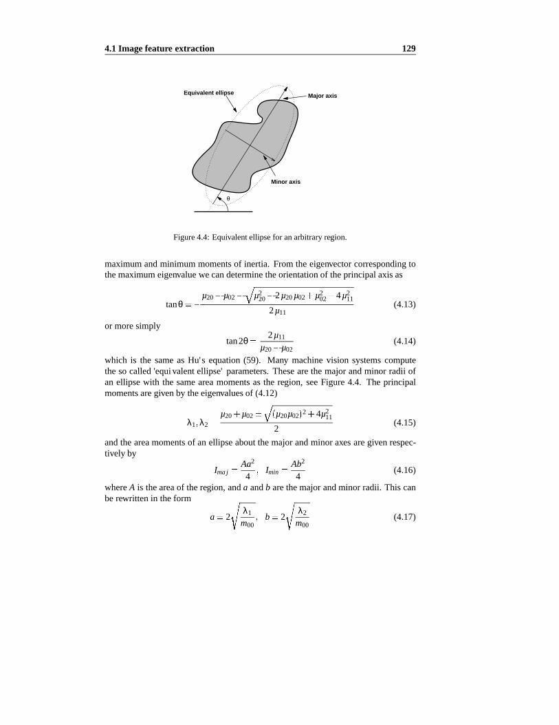
4.1Imagefeature extraction 129
Major axis
Minor axis
Equivalent ellipse
θ
Figure4.4: Equivalentellipsefor anarbitraryregion.
maximumandminimummomentsof inertia. Fromtheeigenvectorcorrespondingtothemaximumeigenvaluewecandeterminetheorientationof theprincipalaxisas
tanθµ20 µ02 µ2
20 2µ20µ02 µ202 4µ2
11
2µ11(4.13)
or moresimply
tan2θ2µ11
µ20 µ02(4.14)
which is the sameas Hu's equation(59). Many machinevision systemscomputethesocalled'equivalentellipse' parameters.Thesearethemajorandminor radii ofan ellipsewith the sameareamomentsasthe region, seeFigure4.4. The principalmomentsaregivenby theeigenvaluesof (4.12)
λ1 λ2
µ20 µ02 µ20µ022 4µ2
11
2(4.15)
andtheareamomentsof anellipseaboutthemajorandminor axesaregivenrespec-tively by
ImajAa2
4Imin
Ab2
4(4.16)
whereA is theareaof theregion,anda andb arethemajorandminor radii. This canberewritten in theform
a 2λ1
m00b 2
λ2
m00(4.17)

130 Machine vision
Thenormalizedmoments
ηpqµpq
µγ00
γ12
p q 1 for p q 2 3 (4.18)
areinvariantto scale.Third-ordermomentsallow for thecreationof quantitiesthatareinvariantwith respectto translation,scalingandorientationwithin a plane.Hu [125]describesa setof sevenmomentinvariants
φ1 η20 η02 (4.19)
φ2 η20 η022 4η2
11 (4.20)
φ3 η30 3η122 3η21 η03
2 (4.21)
φ4 η30 η122 η21 η03
2 (4.22)
φ5 η30 3η12 η30 η12 η30 η122 3 η21 η03
2 (4.23)
3η21 η03 η21 η03 3 η30 η122 η21 η03
2
φ6 η20 η02 η30 η122 η21 η03
2 (4.24)
4η11 η30 η12 η21 η03
φ7 3η21 η03 η30 η12 η30 η122 3 η21 η03
2 (4.25)
3η12 η30 η21 η03 3 η30 η122 η21 η03
2
andHall [105] demonstratesthis invariancefor a numberof realdigital imagesthathave beenscaled,translatedandrotated.Smalldifferencesareobserved in thecom-putedinvariantsandtheseareattributedto thediscretenatureof thedata.
Region momentscanalso be determinedfrom the verticesof a polygonor theperimeterpointsof a boundaryrepresentation[278]. For n boundarypointslabelled1 n wherepointP0 Pn
mpq1
p q 2
n
∑1
Ap
∑i 0
q
∑j 0
1 i j
i j 1pi
qj
xp iyq j ∆xi ∆yj (4.26)
whereA x ∆y y ∆x , ∆x x x 1 and∆y y y 1. An alternativeformu-lation [278] is moresuitablefor computinga fixedsetof momentsduringtraversalofa chain-codedboundary.
4.1.3 Binary regionfeatures
Binary imageprocessingand centroiddeterminationis commonlyusedin field orframeratevision systemsfor visual control. Herewe look at how the estimationofobjectcentroidandwidth areaffectedby threshold,noise,edgegradientandpixel fillfactor. Theanalyticapproachdevelopedherediffersfrom thatgivenby HaralickandShapiro[107] andHo [118] in its explicit modellingof thethresholdingprocess.
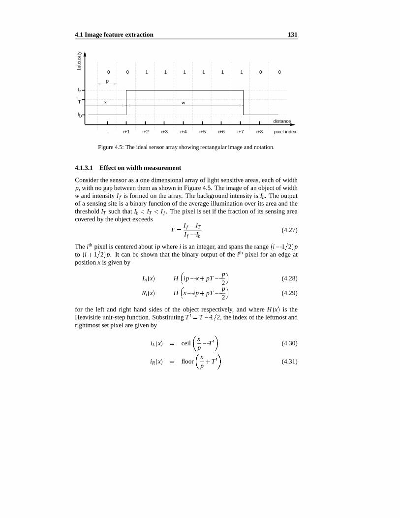
4.1Imagefeature extraction 131
If
Ib
0 0 1 1 1 1 1 1 0 0
x w
distance
i i+1 i+2 i+3 i+4 i+5 i+6 i+7 i+8 pixel index
p
TI
Inte
nsity
Figure4.5: Theidealsensorarrayshowing rectangularimageandnotation.
4.1.3.1 Effect on width measurement
Considerthesensorasa onedimensionalarrayof light sensitiveareas,eachof widthp, with nogapbetweenthemasshown in Figure4.5.Theimageof anobjectof widthw andintensityI f is formedon thearray. Thebackgroundintensityis Ib. Theoutputof a sensingsite is a binaryfunctionof theaverageillumination over its areaandthethresholdIT suchthat Ib IT I f . Thepixel is setif the fractionof its sensingareacoveredby theobjectexceeds
TI f ITI f Ib
(4.27)
The i th pixel is centeredabouti p wherei is aninteger, andspanstherange i 1 2 pto i 1 2 p. It canbe shown that the binaryoutputof the i th pixel for an edgeatpositionx is givenby
Li x H ip x pTp2
(4.28)
Ri x H x ip pTp2
(4.29)
for the left and right handsidesof the object respectively, and whereH x is theHeavisideunit-stepfunction.SubstitutingT T 1 2, theindex of theleftmostandrightmostsetpixel aregivenby
iL x ceilxp
T (4.30)
iR x floorxp
T (4.31)

132 Machine vision
whereceil x is the smallestintegersuchthatceil x x, andfloor x is the largestintegersuchthatfloor x x. Theedgepixel positionsareafunctionof thethresholdused,aswell asthebackgroundandforegroundintensities.
Themeasured,quantized,width is
W x iR x w iL x 1 (4.32)
floorx w
pT ceil
xp
T 1 (4.33)
whichcanbesimplifiedby substitutingfor distancesnormalizedto thepixel width
xxp
wwp
(4.34)
sothat(4.33)becomes
W x floor x w T ceil x T 1 (4.35)
which is a two-valuedfunctionwith a periodof onepixel width, astheobjectmovesacrossthe sensingarray. In order to understandthe distribution of quantizedwidthestimatesit is usefulto substitute
x x x (4.36)
w w w (4.37)
wherex floor x , w floor w , and x w 0 1 . By inspectionit is clearthatfor integervaluesof θ
floor θ x θ floor x (4.38)
ceil θ x θ ceil x (4.39)
soequation(4.35)canberewrittenas
W x floor x w T ceil x T 1 (4.40)
floor x x w w T ceil x x T 1 (4.41)
w 1 floor x w T ceil x T (4.42)
which is a periodictwo-valuedfunctionof x. That is, a singlequantizedwidth mea-surementW switchesbetweentwo valuesthatbrackettheactualwidth w . For manymeasurements,andassumingauniformdistributionfor x, theexpectedvalueof W xcanbeshown to be
E W w w 2T (4.43)
w 2T (4.44)

4.1Imagefeature extraction 133
The averagewidth measurementasthe objectmoveswith respectto the sensingar-ray is dependentupon the thresholdselected. It will give an unbiasedestimateofwidth only whenT 0, or T 1 2. From(4.27)this situationoccursonly whentheintensitythresholdT is midwaybetweentheforegroundandbackgroundintensities.
4.1.3.2 Accuracy of centroid estimate
Using a similar approachthe accuracy of centroiddeterminationin the horizontaldirectioncanbederived.Thequantizedcentroidof theobjectin Figure4.5is
x xiR x w iL x
2(4.45)
12
floor x w T ceil x T (4.46)
12
floor x x w w T ceil x x T (4.47)
12
2x w floor x w T ceil x T (4.48)
which is againa periodictwo-valuedfunction.Theexpectedvalueof x x is
E x12
2x w w 1 (4.49)
xw2
12
(4.50)
andthetruecentroidis
x xw2
(4.51)
sotheexpectedvalueof errorbetweenthemis
E x x 0 (4.52)
indicatingthatthecentroidestimateis anunbiasedestimateof thecentroidandunlikethewidth estimateis independentof threshold.
4.1.3.3 Centroid of a disk
Thecentroidof adiskin thehorizontaldirectioncanbeconsideredtheweightedmeanof the centroidsof eachhorizontalline segmentcomprisingthe imageof the disk.Intuitively we would expect that the larger the disk and the greaterthe numberofline segmentcentroidsaveraged,thecloserthataveragewouldapproachtheexpectedvaluefrom (4.50).Ho [118] discussesthis issueandderivestheapproximation
σ2XC
19π2
4d
1d3 (4.53)

134 Machine vision
If
Ib
T
w
N
distance
Intensity
Figure4.6: Theeffectof edgegradientsonbinarizedwidth.
whered is thedisk'sdiameter. Ravn etal. [13] show asimulationof centroidvarianceasa functionof diskdiameterwhichhasapproximatelythischaracteristic.
4.1.3.4 Effect of edgeintensity gradients
Sofar thethediscussionhasconcentratedonthecasewheretheimagehasarectangu-lar intensityprofile but previoussectionsof this chapterhave discussedmechanismswhich reduceedgesharpnessasshown in Figures3.26and3.27. In a visual servosystemedgegradientmay be further reducedby focuserrorsasthe objectdistancevaries.Theresultingedgemaybemoreaccuratelymodelledasatrapezoidalintensityprofile asshown in Figure4.6. Changesin threshold,∆T , or ambientillumination,∆Ib, will have a markedeffect on thewidth of thebinarizedobject,
∆W 2∆Ib ∆T
ρ(4.54)
whereρ is theedgegradientin unitsof greylevel pixel. In practice,with edgewidthsof up to 5 pixels,this effect will dominateerrorsin themeasuredwidth of thebinaryobject.
4.1.3.5 Effect of signal to noiseratio
Imagenoisesourceswerediscussedin Section3.3.7.Theforegroundandbackgroundimageintensitiesshouldaccuratelybe consideredas randomvariableswith knowndistributions.Providedthatthetwo meansarewell separatedit is possibleto segmentthemusinga fixedthreshold.
Usingthenoisemeasurementdatafor thePulnixcamera,shown in Figure3.18,themaximumvariancecanbetakenas4greylevels2. If a normaldistribution is assumedthen99%of all pixelswill bewithin 6greylevelsof the mean. The probabilityof

4.1Imagefeature extraction 135
a pixel beinggreaterthan 10greylevels from the meanis extremely low, around1pixel from theentire512 512pixel image.
In ascenewith highcontrastandawell chosenthreshold,cameranoiseis unlikelyto bea problem. However practicalissuessuchasunevensceneillumination or thecos4 effect in (3.12)maybringsomepartsof theimagecloseto thethresholdresultingin patchesof binary pixel noise. A conservative rule of thumb would be to keepthe thresholdat least3σ above the backgroundgreylevel andat least3σ below theforegroundgreylevel, keepingin mind thatσ is a functionof intensity.
Cameranoiseon the pixels wherethe edgeintensity crossesthe thresholdwilladduncertaintyto theedgeof thebinary imageandmayevenresultin isolatednoisepixelsadjacentto theedge.Theprobabilityof noisechangingthethresholdoutcomeisinverselyproportionalto theedgegradient.Simplegeometryresultsin anotherruleofthumbthatρ 3σ. For worst-caseobservedcameravarianceof 4, this would requireρ 6greylevel pixel which is easilysatisfied.Figure3.26for exampleshows edgegradientsof at least50greylevel pixel.
Noiseis manifestedassinglepixelsof oppositecolor to their neighbourswhichcanbereadilyeliminatedby a medianfilter. Sucha filter setsthepixel to themedianvalueof all its neighbours.For a binaryimagesucha filter canbeimplementedusingsimplelogic.
4.1.3.6 Numerical simulation
Theanalyticapproachesof Sections4.1.3.1and4.1.3.2becomeintractablewhentry-ing to modeledgegradient,pixel fill factor andadditive noise. Insteada numericalapproachhasbeenusedwhichmodelsatrapezoidalintensityprofilemoving onepixelacrossthesensingarrayin a largenumberof smallstepswhile statisticsaregatheredaboutthemeanwidth andcentroiderror. Conclusionswhich canbedrawn from thesimulationsare:
Thethresholddependenceof meanwidth error, (4.44),is verifiedfor a rectan-gularintensityprofile.
Theeffectof thresholdandintensitychangeonmeanwidth error, (4.54),for thecaseof trapezoidalintensityprofile is verified.
Themeancentroiderror, (4.52),is 0 andindependentof threshold.
Reducingpixel fill factor, h 1, hasno apparenteffect on meanerroror vari-anceof width or centroid.
Additivenoisehasvery little effect onmeancentroidandwidth errorfor a wellchosenthreshold.As thethresholdapproacheseitherforegroundor backgroundintensity, meanwidth error increasesby severalpixels,but meancentroiderroris unaffected.

136 Machine vision
As edgegradientis reducedthemeanwidth andcentroiderrorareunchanged,but thevarianceincreases.
Simulationshave alsobeenperformedto examinetheeffect of objectmotionandfinite exposuretime,Te, onanobjectwith significantedgegradientor anasymmetricintensityprofile. It wasfoundthat,irrespectiveof intensityprofile,thecentroidof thebinarizedblurredimageis the centroidof the binarizedimagehalfway throughtheexposureinterval, asderivedearlierin (3.47). It shouldbenotedin this casethat thecentroidof thebinary imagedoesnot correspondto thecentroidof theobject if theintensityprofile is asymmetric.
4.1.3.7 Summary
For accuratedeterminationof distancewith apossiblyunfocussedcamerait is prefer-abletousethedistancebetweencentroidsof featuresratherthanthewidthof afeature.The latter is significantlyaffectedby variation in thresholdand illumination whenedgesarewide. Alexander[6] hasshown, in the context of cameracalibration,thatspatialaliasingdueto imagesharpnesscanin fact introducea small but systematicerrorin centroiddetermination.Heshowshow thismaybeminimizedby introducingdiffractionblur. Giventhepooredgeresponseof thelensusedin this work problemsdueto excessive imagesharpnessarenot expectedto be significant. It canbe con-cludedthat if centroidsof imagefeaturesareusedit is not necessaryto have a sharpimagesincethecentroidestimateis unbiased.
4.1.4 Feature tracking
Softwarecomputationof imagemomentsis oneto two ordersof magnitudeslowerthanspecializedhardware.However thecomputationtime canbegreatlyreducedifonly asmallimagewindow, whoselocationis predictedfrom thepreviouscentroid,isprocessed[77,92,99,108,212,274]. Thetaskof locatingfeaturesin sequentialscenesis relativelyeasysincetherewill beonlysmallchangesfromonesceneto thenext [77,193] andtotal sceneinterpretationis not required.This is theprincipleof verificationvisionproposedby Bolles[34] in whichthesystemhasconsiderableprior knowledgeof thescene,andthegoal is to verify andrefinethe locationof oneor morefeaturesin thescene.Determiningthe initial locationof featuresrequirestheentireimagetobe searched,but this needonly be doneonce. Papanikolopouloset al. [197] useasum-of-squareddifferencesapproachto matchfeaturesbetweenconsecutive frames.Featuresarechosenon thebasisof a confidencemeasurecomputedfrom thefeaturewindow, and the searchis performedin software. The TRIAX system[19] is anextremelyhigh-performancemultiprocessorsystemfor low latency six-dimensionalobjecttracking. It candeterminethe poseof a cubeby searchingshortchecklinesnormalto theexpectededgesof thecube.

4.2Perspectiveand photogrammetry 137
Whenthesoftwarefeaturesearchis limited to only a smallwindow into the im-age,it becomesimportantto know theexpectedpositionof the featurein the image.This is the target trackingproblem; the useof a filtering processto generatetargetstateestimatesandpredictionsbasedon noisy observationsof the target's positionanda dynamicmodelof the target's motion. Target maneuversaregeneratedby ac-celerationcontrolsunknown to the tracker. Kalata [141] introducestrackingfiltersanddiscussesthesimilaritiesto Kalmanfiltering. Visualservoing systemshave beenreportedusingtrackingfilters [8], Kalmanfilters [77,274], AR (autoregressive) orARX (autoregressive with exogenousinputs)models[91,124]. Papanikolopoulosetal. [197] useanARMAX modelandconsidertrackingasthedesignof asecond-ordercontrollerof imageplaneposition.Thedistanceto thetargetis assumedconstantanda numberof differentcontrollerssuchasPI, pole-assignmentandLQG are investi-gated.For thecasewheretargetdistanceis unknownor time-varyingadaptivecontrolis proposed[196]. Thepredictionusedfor searchwindow placementcanalsobeusedto overcomelatency in thevisionsystemandrobotcontroller.
Dickmanns[77] andInoue[128] have built multiprocessorsystemswhereeachprocessoris dedicatedto trackinga singledistinctive featurewithin theimage.Morerecently, Inoue[129] hasdemonstratedtheuseof a specializedVLSI motionestima-tion device for fastfeaturetracking.
4.2 Perspectiveand photogrammetry
Theperspectivetransforminvolvedin imagingwasintroducedin Section3.2.4andthelensequationsin pixel coordinatesas(3.66)and(3.67). Usinghomogeneouscoordi-natesthis non-lineartransformationmaybeexpressedin linear form for anarbitrarycameralocation.Usingmatrix representationtheoverall cameratransformationis:
ixiyiz
αx 0 X0 00 αy Y0 00 0 1 0
1 0 0 00 1 0 00 0 1 f 10 0 0 1
0Tc1
xyz1
(4.55)
whereαx X-axisscalingfactorin pixels/mm(intrinsic)αy Y-axisscalingfactorin pixels/mm(intrinsic)X0 imageplaneoffsetin pixels(intrinsic)Y0 imageplaneoffsetin pixels(intrinsic)f focal length(intrinsic)
0Tc camerapositionin world coordinates(extrinsic),seeFigure4.7.The imageplanecoordinatesin pixelsare thenexpressedin termsof homogeneous

138 Machine vision
coordinatesas
iXixiz
(4.56)
iYiyiz
(4.57)
in unitsof pixels.Intrinsic parametersareinnatecharacteristicsof thecameraandsensor, while ex-
trinsic parametersarecharacteristicsonly of thepositionandorientationof thecam-era. The principal point is the intersectionof the optical axis andthe CCD sensorplane,atpixel coordinatesX0 Y0 .
Therelevanttransformationsandcoordinateframesareshown in Figure4.7. cTP
is thepositionof theobjectwith respectto thecamera.Otherrelationshipsinclude
0TP0Tc
cTP (4.58)cTP
0Tc1 0TP (4.59)
whichallow (4.55)to bewrittencompactlyas
ixiyiz
C
xyz1
(4.60)
whereC is the camera calibration matrix, a 3 4 homogeneoustransformwhichperformsscaling,translationandperspective. C representstherelationshipbetween3-D world coordinatesandtheir corresponding2-D imagecoordinatesasseenby thecomputer.
Equation(4.55)maybeexpandedsymbolically. With theinversecamerapositiontransformrepresentedin directionvectorform cT0 n o a p wecanderive
C
αx nx f X0nzf cz
αx ox f X0ozf cz
αx ax f X0azf cz
αx cx f X0cz X0 ff cz
αy ny f Y0nzf cz
αy oy f Y0ozf cz
αy ay f Y0azf cz
αy cy f Y0cz Y0 ff cz
nzf cz
ozf cz
azf cz
1
(4.61)
4.2.1 Close-rangephotogrammetry
Photogrammetryis the scienceof obtaininginformationaboutphysicalobjectsviaphotographicimages,andis commonlyusedfor makingmapsfromaerialphotographs[282]. Close-range,or terrestrial,photogrammetryis concernedwith objectdistanceslessthan100m from thecamera.Much nomenclaturefrom this disciplineis usedintheliteraturerelatedto cameracalibrationand3D vision techniques.

4.2Perspectiveand photogrammetry 139
P
Z
Y
XTP
Tc
PTc
0
C
Figure4.7: Relevantcoordinateframes.
A metriccamerais purposebuilt for photogrammetricuseandis bothstableandcalibrated.The calibrationparametersincludethe focal length, lensdistortion,andthecoordinatesof theprincipalpoint. A metriccamerahasfiducial markswhich arerecordedon thephotographsuchthatlinesjoining oppositefiducialmarksintersectattheprincipalpoint.
A nonmetriccamerais one manufacturedfor photographicuse, wherepicturequality, not geometry, is important. Nonmetriccamerascanbe calibratedandusedfor lessdemandingphotogrammetricapplicationssuchasmachinevision.
4.2.2 Cameracalibration techniques
Cameracalibrationis the processof determiningthe internalcamerageometricandoptical characteristics(intrinsic parameters)andthe 3-D positionandorientationofthecameraframerelative to a certainworld coordinatesystem(extrinsicparameters).Frequentlyit is usefulto empiricallydeterminethecameracalibrationmatrix whichrelatesa world coordinatesystemto the imageplanecoordinates[27] for a givencamerapositionandorientation.
The importantcharacteristicsof a numberof calibrationtechniquesaresumma-rizedin Table4.1. They differ in their ability to calibratelensdistortion,andthetypeof calibrationtarget required. Chartswith coplanarpointscanbe generatedconve-

140 Machine vision
Figure4.8: The SHAPEcalibrationtarget usedfor intrinsic parameterdetermi-nation. The surfaceis brushedaluminiumwith black markerdotsat accuratelyknown locationson thetwo surfaces.

4.2Perspectiveand photogrammetry 141
Method Targettype DistortionCoplanar Non-coplanar
ClassicnonlinearHomogeneoustransform2 planes2 stage
Table4.1: Comparisonof themajorfeaturesof differentcameracalibrationtechniques.
niently andaccurately1 usinga laserprinter. Circularmarksarefrequentlyusedforcentroiddeterminationbut errorswill beintroducedif thesearenot viewedalongthesurfacenormal. In thatcase,asshown earlierin Figure4.3,thecentroidof theimage(which will beanellipse)will not correspondwith thecentroidof the marker. Thiseffect canbeminimizedby keepingthemarksizesmall(imagesizeof a few pixels),usinga crossshapedtarget,or usingthecornersof rectangularmarkers.Calibrationusingnon-coplanarpointsrequiresa mechanicallycomplex calibrationframesuchasthatshown in Figure4.8,or motionof a robotto positiona calibrationmarkwith re-spectto thecamera.Experimentsconductedusingtherobotresultedin largeresidualsandthis is suspectedto bedueto low positioningaccuracy. Thenext sectionsbrieflydescribethedifferentapproachesto cameracalibrationandpresentsomeexperimentalresults.
4.2.2.1 Classicalnon-linear approach
Techniquesin this category have beendevelopedin thephotogrammetriccommunityandareamongstthe oldestpublishedreferences[87,239,282,283]. The cameraisdescribedby a detailedmodel,with in somecasesup to 18 parameters.Non-linearoptimizationtechniquesusethecalibrationdatato iterativelyadjustthemodelparam-eters.
4.2.2.2 Homogeneoustransformation approach
Approachesbasedon thehomogeneoustransformation[27,243] allow directestima-tion of thecalibrationmatrixC in (4.60).Theelementsof this matrixarecompositesof the intrinsic and extrinsic parameters.Lensdistortion cannotbe representedinlinearhomogeneousequations,but this canbecorrectedin a separatecomputationalstep.
Expandingequations(4.60)-(4.57)wemaywrite
C11x C12y C13z C14 C31iXx C32
iXy C33iXz C34
iX 0 (4.62)
1Lessthan1%scaleerrormeasuredin thepaperfeeddirection.

142 Machine vision
Imageplane
Calibrationplane 1
Calibrationplane 2
y y
x
Y
X
xz1 z
2
Figure4.9: Thetwo-planecameramodel.
C21x C22y C23z C24 C31iYx C32
iYy C33iYz C34
iY 0 (4.63)
which relateanobservedimagecoordinate iX iY to a world coordinate x y z . Forn observationsthis maybeexpressedin matrix form asa homogeneousequation
x1 y1 z1 1 0 0 0 0 iX1x1iX1y1
iX1z10 0 0 0 x1 y1 z1 1 iY1x1
iY1y1iY1z1
...xn yn zn n 0 0 0 0 iXnxn
iXnyniXnzn
0 0 0 0 xn yn zn n iYnxniYnyn
iYnzn
C11C12
...C33
iX1iY1...
iXniYn
(4.64)
A non-trivial solutioncanonly beobtainedto within a scalefactorandby conventionC34 is setequalto 1. Equation(4.64)has11 unknownsandfor solutionrequiresatleast5.5 observations(pairsof iX iY and x y z of non-coplanarpointsfor solu-tion2. Thissystemof equationswill generallybeover determined,anda leastsquaressolutionmaybeobtainedusinga techniquesuchassingularvaluedecomposition.
2Coplanarpointsresultin theleft-handmatrixof (4.64)becomingrankdeficient.

4.2Perspectiveand photogrammetry 143
4.2.2.3 Two-planecalibration
The homogeneoustransformapproachis basedon the pinholecameramodel, andcannotbereadilyextendedto dealwith lensdistortions.Thetwo planeapproachhasbeensuggested[180] to overcomethis limitation. As shown in Figure4.9, a line inspaceis definedby a pointoneachof two calibrationplanes,givenby
xyz k
AkiXn iXn 1iY iYn iX iY 1
T(4.65)
whereAk is the interpolationmatrix for calibrationplanek. The two planemethodallowsfor rapidcomputationof inverseperspective,thatis,3D linesfrom imageplanepoints.Theline is obtainedby interpolatingthe3D world coordinatescorrespondingto theimageplanecoordinatefor thetwo calibrationplanes.
Theinterpolationmatrixfor eachplanemaybedeterminedbyplacingatestpatterncontainingan arrayof dotsat a known distancefrom the camera.The orderof theinterpolationshouldbechosento balancecomputationtime,accuracy andstability—in practicesecondor third orderis sufficient[130]. Theinterpolationmatriximplicitlycorrectsfor lensdistortion.
4.2.2.4 Two-stagecalibration
Thetwo-stagecalibrationschemeof Tsai[252] canbeusedto determinetheintrinsicandextrinsic cameraparametersfrom a singleview of a planarcalibrationtarget. Itrelieson theso-called'radialalignmentconstraint'whichembodiesthefact that lensdistortionactsalongradiallinesfrom theprincipalpoint. Thealgorithmis moderatelycomplex, but is claimedto executevery quickly. It doesrequireprior knowledgeofthedigitizerto cameraclockratio,β, andthepixel scalingfactorsαx andαy, aswell asthecoordinatesof theprincipalpoint. Tsaiconsidersthis latterparameterunimportantandsetsit arbitrarily to thecoordinateof thecenterof theframestore.As foundlater,theprincipalpoint for thiscameraanddigitizer is somedistancefrom thecenter.
Considerabledifficulty was experiencedusing Tsai's method,and in particularit proved to very sensitive to slight changesin the parameterβ andprincipal pointcoordinate. Anecdotalevidencefrom other researchersandalso[210] suggestthatthis experienceis not uncommon.Onepossiblereasonfor thedifficulty encounteredis that the lenshasinsufficient radial distortion,thoughthis would be surprisingforsuchashortfocal lengthlens.
4.2.2.5 Decomposingthe cameracalibration matrix
The homogeneouscameracalibrationmatrix, C, containsinformationaboutthe po-sition of the camerawith respectto the world coordinateframe,aswell asintrinsic

144 Machine vision
parametersof thecamera.Determiningtheextrinsic parametersis alsoreferredto asthecamera locationdeterminationproblem.
Theline of sightof thecamerain world coordinatescanbedeterminedasfollows.For agivenimageplanepoint iX iY wecanwrite
C11iXC31 x C12
iXC32 y C13iXC31 z iXC34 C14 (4.66)
C21iYC31 x C22
iYC32 y C23iYC31 z iYC34 C24 (4.67)
which arethe equationsof two planesin world space,onevertical correspondingtoconstantiX in the imageplane,andonehorizontal.The intersectionof theseplanesis the line in 3D spacethat is mappedto that imageplanepoint3. A directionvectorparallelto this intersectionline is foundvia crossproduct
x y zC11
iXC31 C12iXC32 C13
iXC31
C21iYC31 C22
iYC32 C23iYC31
(4.68)
SubstitutingiX X0 and iY Y0 gives a direction vector parallel to the camera'soptical axis. However X0 andY0 are intrinsic calibrationparametersandcannotbeassumedto bethecenterof thesensingarray[169].
Alternatively the lens law singularitymay be usedto definethe camera's focalplane,thatis z f . Thefocal planeis givenby
C31x C32y C33z 0 (4.69)
andthecameraaxisdirectionvectoris normalto this plane,parallelto thevector
C31x C32y C33z (4.70)
Strat[242] extendstheapproachof (4.69)to alsodeterminecamerapositionandrollabouttheopticalaxis.
Thecalibrationmatrix, C, encodesthe6 extrinsic parameters4 and5 intrinsicpa-rameters:f , αx, αy, X0 andY0. However it is not possibleto uniquelydetermineallthe intrinsic parameters,only theproductsf αx and f αy
5. This leaves10 parametersto be determinedfrom 11 elementsof the cameracalibrationmatrix which is overdetermined,leadingto difficulties in solution. Ganapathy[97] describesa sophisti-catedprocedurefor determiningtheintrinsicandextrinsic parametersby introducinganotherparameter, δ, aqualitymeasurein unitsof degreeswhichis ideallyzero.Thisis interpretedas error in the orthogonalityof the imageplaneX andY axes. Theapproachis robustto inaccuraciesin thecalibrationmatrix.
3Equations(4.66)and(4.67)represent2 equationsin 3 unknowns.Fromtwo cameraviewsof thesamepoint,wearethenableto solvefor the3D locationof thepoint — thebasisof stereovision.
43D positionvectorand3 anglesfor camerapose.5Fromthesymbolicexpansionof (4.61)it canbeseenthatonly theproductsf αx and f αy appear.

4.2Perspectiveand photogrammetry 145
Givena numericalvaluefor C it is alsopossibleusinggradientsearchtechniquesto find thevaluesof theintrinsicandextrinsicparameters.In practicethisapproachisfoundto bequitesensitive to choiceof initial valuesandcansettlein localminima.
4.2.2.6 Experimental results
Four imagesof theSHAPEcalibrationtarget,shown in Figure4.8,weretakenfromdifferentviewpoints.Eachtime thefocusandaperturewereadjustedfor imagesharp-nessandbrightness.Thecentroidof eachmarkerwasdeterminedto sub-pixel preci-sionby computinganintensityweightedaverageof pixel coordinatesin theregion ofthemarker. As shown in Figure4.10theintensityprofileof amarkeris abroadflat hillnot a stepfunction,andthis would beexpectedfrom theearlierdiscussionregardingimageMTF. Thecentroiddeterminationprocedureusedis asfollows:
1. An imagedisplayutility wasusedto manuallydeterminethe locationof eachmarkto within 5 pixels.Thetargetwasdifficult to light evenlydueto its com-plex shape,makingit infeasibleto automaticallyandrobustlyfind themarkers.
2. The lowest6 intensitypixel within a 10 x 10 region of eachmanuallyselectedpointwaslocated.Thispointwill bereferredto asthecenterpoint xc yc .
3. The averagebackgroundintensity, Ib, wascomputedfrom the intensityat thefour cornersof a squarewindow aboutthecenterpoint.
4. Averagebackgroundintensitywassubtractedfrom all pixels in theregion andtheweightedaveragecoordinatescomputed
xΣiΣ j i Ii j IbΣiΣ j Ii j Ib
(4.71)
yΣiΣ j j Ii j IbΣiΣ j Ii j Ib
(4.72)
A programwaswritten to automatetheselastthreesteps.Usingknown 3D markerlocationandthecorrespondingimageplanecoordinates
thecalibrationmatrixwascomputedby solving(4.64)usingsingularvaluedecompo-sition. TheresultingmatrixwasthendecomposedusingGanapathy'smethodandtheresultsaresummarizedin Table4.2. Residualis the maximumresidualafter substi-tuting thecalibrationmatrixparametersbackinto (4.64).δ is thequality factordeter-minedby Ganapathy'salgorithmandshouldideally bezero.Theremainingcolumnsshow intrinsicparametersderivedby Ganapathy'smethod.Thereis somevariationintheprincipalpointcoordinateandalsothescalefactors.Howevertheratioof thescale
6Thecalibrationmarkswereblackonwhite.

146 Machine vision
1 2 3 4 5 6 7 8 9 101
2
3
4
5
6
7
8
9
10
X
Y
Figure4.10:Contourplot of intensityprofilearounda typicalcalibrationmarker.Dueto overallMTF theedgesof themarkerdotarenotsharp.
Trial Residual δ X0 Y0 αx f αy f αy αx
(pixel) (deg) (pixel) (pixel) (pixel) (pixel)
1 0.552 -0.0277 270.1 213.7 625.7 948.9 1.522 0.898 0.0672 271.4 223.1 614.0 933.0 1.523 0.605 0.0685 278.0 205.6 617.3 938.2 1.524 0.639 -0.1198 275.8 196.8 616.8 939.2 1.52
mean 273.8 209.8 615.5 939.8σ 3.2 9.7 5.0 6.6
Table4.2: Summaryof calibrationexperimentresults.
factorsis constantat 1 52which is alsothevaluedeterminedin Section3.5.3.Usingthepixel scalefactordatafrom Table3.8thefocal lengthis estimatedas7 8mm. Thisis marginally lowerthan8mm,thenominalfocal lengthof thelens,but within the4%toleranceof ANSI StandardPH3.13-1958“Focal LengthMarking of Lenses”. TheY-coordinateof the principal point is found to bewell above the centerof the pixelarray. This effect couldbeexplainedby theplacementof theCCD sensorwithin thecameraat theappropriatepoint for anRS170ratherthanCCIR image.

4.2Perspectiveand photogrammetry 147
Many researchershave observed extremesensitivity in the cameracalibrationtochangesin focusandaperturesetting.Changesin thesesettingscauselenselementstorotate,whichcompoundedwith asymmetriesin thelensalterthescalingandpositionof theimage.Thismayaccountfor someof thevariationobservedsincethelenswasre-adjustedfor eachtrial.
The procedurepresentedis not capableof explicitly modelling geometriclensdistortion,andits effect will introduceerrorsinto the othercameraparameters.Anexperimentwasconductedin whichanarrayof dots,evenlyspacedacrossthefield ofview, wasimagedandtheircentroidscomputed.Themagnitudeof centroiddeviationfrom theline of bestfit waslessthanonepixel with thelargesterrorsoccurringat theedgeof thefield of view.
4.2.3 Eye-handcalibration
Roboteye to handcalibrationis the processof determiningthefixed transformationbetweenthegripperandthecameracoordinatesystem.A numberof approacheshavebeendescribedin theliterature[132,233,253].Generallythey involvetherobotmak-ing anumberof movesandmeasuringthechangein imageplanecoordinatesof afixedtarget.A fairly complex algorithmis thenappliedto determinethecameratransform.Tsai's method[253] againreliesonuseof theplanarcalibrationtarget,andgiventhedifficultiesabove,wasnot tried.
A morepragmaticapproachis to determinethetransformfrom theknown geom-etry of the camera,robot wrist and lens,as shown in Figure4.11. The locationoftheCCDsensorplanewithin thecamerais notdirectlymeasurable.However thelensmanufacturer's datashows thatthefocal pointof thelensis 17.5mmbehindthemat-ing surface,andtheplaneof anequivalentsimplelenswill belocatedthefocal lengthin front of that, seeFigure4.127. From this datathe distanced2 canbe inferredas20.0mm.
The coordinateframeof the camerais alsoshown in Figure4.11. TheX-axis isout of thepage.Thetransformcanbeexpressedin termsof elementaryrotationsandtranslationsas
6Tc TZ d1 RX 90 TZ d2
1 0 0 00 0 1 200 1 0 1210 0 0 1
(4.73)
7A lenssuchasthis, in which thelensplaneis not within thebodyof the lens,andcloseto theimageplane,is referredto asa retrofocuslens.

148 Machine vision
Puma wrist
Pulnix camera
Puma wrist flangeCamera adaptor
center of wrist (T6 point)
Cosmicar lens (C814)
56.25
38
26.5
29.5
d2
optical axis
TCAM6
Lens plane
Y
Zc
Yc
d1
60
Z56
56Z4
Figure4.11:Detailsof cameramounting(not to scale,dimensionsin mm). Robotwrist is in thezeroanglepose.

4.2Perspectiveand photogrammetry 149
17.58
CCD sensor
Lensplane
Equivalent simple lens
back focaldistance
Matingsurface
Figure4.12:Detailsof camera,lensandsensorplacement.

150 Machine vision

Chapter 5
Visual servoing
With this chapterwe start the discussionaboutvisual servoing, that is, how visualfeaturesmay beusedto guidea robotmanipulatoror mechanism.The reporteduseof visual informationto guiderobots,or moregenerallymechanisms,is quiteexten-siveandencompassesapplicationsasdiverseasmanufacturing,teleoperation,missiletrackingcamerasandfruit picking aswell asrobotic ping-pong,juggling, catchingandbalancing.
Section5.1 introducesthe topic of visual servoing and introducesa consistentterminologythatwill beemployedthroughout,allowing discussionof papersdespitethe differentnomenclatureusedby the authors.The sectionalsointroducesthe twowell known approachesto visualservoing: position-basedandimage-based.A moreformal treatmentof thefundamentalsis givenby Hageret al. [103].
Themajorityof priorworkconcentratesonthe'classical' issuesin visualservoing,referredto in [52] asvisual servokinematics. This is concernedwith the kinematicrelationshipbetweenobjectpose,robotposeandimageplanefeatureswithout regardto dynamiceffects.However controlstrategiesbasedpurelyon kinematicconsidera-tionsareonly adequatefor low-performanceapplications.Visual servodynamics, ontheotherhand,is concernedwith thedynamicsor motionof thevisualservo systemandissuessuchasstability, settlingtimeandtrackinglags.This chapterconcentrateslargelyonkinematicissues,while thefollowingchaptersaddressdynamics,modellingandcontrol.
Section5.2 providesa comprehensive review of prior work on the topic of vi-sualservoing. Sections5.3 and5.4 discussrespectively the detailsof position-andimage-basedtechniques.Miscellaneousissuesrelatingto implementationandarchi-
An early versionof this chapterwas publishedas [59] “Visual control of robot manipulators— areview” in K. Hashimoto,editor, Visual Servoing, volume7 of Roboticsand AutomatedSystems, pages1–31.World Scientific,1993.
151

152 Visual servoing
xct
x t
P
xce
xe
Figure5.1: Relevantcoordinateframes;world,end-effector, cameraandtarget.
tecturesarereviewedin Section5.5.Necessarilywith this structurethework of someresearcherswill bereferredto severaltimes,but in differentcontexts.
5.1 Fundamentals
Thetaskin visualservoing is to controltheposeof therobot'send-effector, xt6, usingvisual information,features, extractedfrom the image2. Pose,x, is representedby asix elementvectorencodingpositionandorientationin 3D space.The cameramaybefixed,or mountedon therobot'send-effectorin whichcasethereexistsa constantrelationship,t6xc, betweenthe poseof the cameraand the poseof the end-effector.Theimageof thetarget3 is a functionof therelativeposebetweenthecameraandthetarget,cxt . Therelationshipbetweentheseposesis shown in Figure5.1.Thedistancebetweenthecameraandtarget is frequentlyreferredto asdepthor range.
Thecameracontainsa lenswhichformsa2D projectionof thesceneontheimageplanewherethesensoris located.This projectioncausesdirectdepthinformationtobe lost, andeachpoint on the imageplanecorrespondsto a ray in 3D space.Someadditionalinformationis neededto determinethe3D coordinatecorrespondingto animageplanepoint. This informationmaycomefrom multipleviews,or knowledgeofthegeometricrelationshipbetweenseveralfeaturepointson thetarget.
2Thetaskcanalsobedefinedfor mobilerobots,whereit becomesthecontrolof thevehicle'sposewithrespectto somelandmarks.
3Theword targetwill beusedto referto theobjectof interest,thatis, theobjectwhich will betracked.

5.1Fundamentals 153
An imagefeature, Section4.1,is a scalaror vectorquantityderivedfrom somevi-sualfeatureor featuresin theimage.Commonlythecoordinateof someeasilydistin-guishablepoint,or aregion centroidis used.A featurevector, f , is aonedimensionalvectorcontainingfeatureinformationasdescribedabove. A goodvisualfeatureis onethatcanbelocatedunambiguouslyin differentviews of thescene,suchasa holein agasket[91,92]or acontrivedpattern[71,211].Theimageplanecoordinatesof threeormorevisualfeaturescanbeusedto determinethepose(not necessarilyuniquely, seeSection5.3.1)of the target relative to thecamera,givenknowledgeof thegeometricrelationshipbetweenthefeaturepoints.
Robotstypically have 6 degreesof freedom(DOF), allowing the end-effector toachieve, within limits, any posein 3D space.Visualservoing systemsmaycontrol6or fewer DOF. Planarpositioninginvolvesonly 2-DOFcontrolandmaybesufficientfor someapplications.Motion soasto keeponepoint in thescene,theinterestpoint,at thesamelocationin theimageplaneis referredto asfixation. Animalsusefixationto direct thehigh resolutionfoveaof the eye towardregionsof interestin thescene.In humansthis low-level, unconscious,fixation motion is controlledby the brain'smedullaregion usingvisual feedbackfrom theretina[5]. Keepingthe targetcentredin thefield of view hasa numberof advantagesthatinclude:
eliminatingmotionblur sincethetarget is not moving with respectto thecam-era;
reducingthe effect of geometricdistortion in the lensby keepingthe opticalaxispointedat thetarget;
minimizing the effect of the cos4 term in (3.12) sincethe angleconcernediscloseto zero.
Fixationmaybeachievedby controllingthepan/tiltanglesof thecameralike ahumaneye,or by moving thecamerain aplanenormalto theopticalaxis.High performancefixationcontrolis animportantcomponentof many activevisionstrategies.
In 1980SandersonandWeiss[223] introducedanimportantclassificationof visualservo structures,andtheseareshown schematicallyin Figures5.2to 5.5. In position-basedcontrol, featuresareextractedfrom the imageandusedin conjunctionwith ageometricmodelof the target to determinetheposeof the targetwith respectto thecamera. In image-basedservoing the last stepis omitted,andservoing is doneonthe basisof imagefeaturesdirectly. The structuresreferredto asdynamiclook andmovemakeuseof joint feedback,whereasthePBVSandIBVS structuresusenojointpositioninformationatall. It is importantto notethatalmostnoneof thevisualservosystemsreportedin the literatueare 'visual servo' systemsaccordingto the Weisstaxonomy, but ratherareof the'dynamiclook andmove' structure.However theterm'visualservoing' is widely usedfor any systemthatusesa machinevision systemtoclosea position-control loop.

154 Visual servoing
+
−
f
Power amplifiers
Imagefeatureextraction
Robot
Camera
video
Joint controllers
joint angle sensors
Poseestimation
xc
dcx Cartesian
control law
Figure5.2: Dynamicposition-basedlook-and-movestructure.
+
−
f
fd
Power amplifiers
Imagefeatureextraction
Robot
Camera
video
Joint controllers
joint angle sensors
Feature spacecontrol law
Figure5.3: Dynamicimage-basedlook-and-movestructure.
Theimage-basedapproachmayreducecomputationaldelay, eliminatetheneces-sity for imageinterpretationandeliminateerrorsin sensormodellingandcameracal-ibration.However it doespresentasignificantchallengeto controllerdesignsincetheplantis non-linearandhighly coupled.
5.2 Prior work
This sectionsummarizesresearchandapplicationsof visual servoing, from the pi-oneeringwork of the early 1970sto the presentday. The discussionis generallychronological,but relatedapplicationsor approacheswill be groupedtogether. Thereportedapplicationsarequiteextensive,encompassingmanufacturing,teleoperation,

5.2Prior work 155
+
−
f
Power amplifiers
Imagefeatureextraction
Robot
Camera
videoPoseestimation
xc
dcx Cartesian
control law
Figure5.4: Position-basedvisualservo (PBVS)structureasperWeiss.
+
−
f
fd
Power amplifiers
Imagefeatureextraction
Robot
Camera
video
Feature spacecontrol law
Figure5.5: Image-basedvisualservo (IBVS) structureasperWeiss.
missiletrackingcamerasandfruit pickingaswell asroboticping-pong,juggling,andbalancing.Dueto technologicallimitationsof the time someof thesignificantearlywork fails to meetthestrictdefinitionof visualservoinggivenearlier, andwouldnowbeclassedaslook-then-moverobotcontrol. Progresshashowever beenrapid,andbythe endof the 1970ssystemshadbeendemonstratedwhich werecapableof 10Hzservoing and3D positioncontrol for tracking,seamwelding andgraspingmovingtargets.
Oneof theearliestreferencesis by ShiraiandInoue[232] in 1973who describehow a visual feedbackloop canbeusedto correctthepositionof a robotto increasetaskaccuracy. A systemis describedwhich allows a robot to graspa squareprismandplaceit in a box usingvisualservoing. Edgeextractionandline fitting areusedto determinethepositionandorientationof thebox. Thecamerais fixed,anda servo

156 Visual servoing
cycle timeof 10sis reported.Considerablework on the useof visual servoing wasconductedat SRI Interna-
tional during the late1970s.Early work [215,216] describestheuseof visual feed-backfor bolt-insertionandpickingmoving partsfrom aconveyor. Hill andPark [116]describevisual servoing of a Unimaterobot in 1979. Binary imageprocessingisusedfor speedandreliability, providing planarpositionaswell assimpledepthes-timationbasedon theapparentdistancebetweenknown features.Experimentswerealsoconductedusinga projectedlight stripeto providemorerobustdepthdetermina-tion aswell assurfaceorientation. Theseexperimentsdemonstratedplanarand3Dvisually-guidedmotion,aswell astrackingandgraspingof moving parts.They alsoinvestigatedsomeof thedynamicissuesinvolvedin closed-loopvisualcontrol.Simi-lar work onaUnimate-basedvisual-servo systemis discussedlaterby Makhlin [179].Prajoux[207] demonstratedvisual servoing of a 2-DOF mechanismfor following aswinginghook. The systemuseda predictorto estimatethe future positionof thehook,andachieved settlingtimesof theorderof 1s. CoulonandNougaret[68] ad-dresssimilarissuesandalsoprovideadetailedimagingmodelfor thevidiconsensor'smemoryeffect. They describea digital videoprocessingsystemfor determiningthelocationof onetargetwithin aprocessingwindow, andusethis informationfor closed-looppositioncontrolof anXY mechanismto achieveasettlingtimeof around0.2stoa stepdemand.
Simplehand-heldlight stripersof thetypeproposedby Agin [3] have beenusedinplanarapplicationssuchasconnectoracquisition[187],weldseamtracking[49], andsealantapplication[227]. Thelast laysa beadat 400mm swith respectto a movingcar-body, andshows a closed-loopbandwidthof 4.5Hz. More recentlyVenkatesanandArchibald [258] describethe useof two hand-heldlaserscannersfor real-time5-DOFrobotcontrol.
Gilbert [101] describesanautomaticrocket-trackingcamerawhich keepsthetar-get centredin the camera's imageplaneby meansof pan/tilt controls. The systemusesvideo-rateimageprocessinghardwareto identify thetargetandupdatethecam-eraorientationat 60Hz. Dzialo andSchalkoff [81] discusstheeffectsof perspectiveon thecontrolof a pan-tilt cameraheadfor tracking.
Weiss[273] proposedtheuseof adaptive control for the non-lineartime varyingrelationshipbetweenrobotposeandimagefeaturesin image-basedservoing. Detailedsimulationsof image-basedvisualservoingaredescribedfor a varietyof manipulatorstructuresof up to 3-DOF.
Weberand Hollis [271] developeda high-bandwidthplanar-positioncontrolledmicro-manipulator. It is requiredto counterroom androbot motor vibrationeffectswith respectto theworkpiecein aprecisionmanufacturingtask.Correlationis usedtotrackworkpiecetexture.To achieve ahighsamplerateof 300Hz, yetmaintainresolu-tion, two orthogonallinearCCDsareusedto observe projectionsof theimage.Sincethesamplerateis hightheimageshift betweensamplesis smallwhichreducesthesize

5.2Prior work 157
of thecorrelationwindow needed.Imageprojectionsarealsousedby Kabuka[137].Fourierphasedifferencesin thevertical andhorizontalbinary imageprojectionsareusedfor centeringa target in the imageplaneanddeterminingits rotation. This isappliedto thecontrol of a two-axiscameraplatform[137] which takes30s to settleon a target. An extensionto this approach[139] usesadaptive control techniquestominimizeperformanceindiceson grey-scaleprojections.The approachis presentedgenerallybut with simulationsfor planarpositioningonly.
An applicationto roadvehicleguidanceis describedby Dickmanns[76]. Real-time featuretrackingandgazecontrolledcamerasguidea 5tonneexperimentalroadvehicle at speedsof up to 96km h along a test track. Later work by Dickmanns[78] investigatesthe applicationof dynamicvision to aircraft landing. Control ofunderwaterrobotsusingvisualreferencepointshasbeenproposedby NegahdaripourandFox [191].
Visually guidedmachineshave beenbuilt to emulatehumanskills at ping-pong[17,88], juggling[212], invertedpendulumbalancing[13,76], catching[41,220],andcontrollinga labyrinthgame[13]. Thelatter is a woodenboardmountedon gimbalson which a ball bearingrolls, theaim beingto move theball througha mazeandnotfall into a hole.Theping-pongplayingrobot[17] doesnotusevisualservoing, ratheramodelof theball's trajectoryis built andinput to adynamicpathplanningalgorithmwhichattemptsto striketheball.
Visualservoing hasalsobeenproposedfor catchingflying objectson Earthor inspace.Bukowski et al. [39] reporttheuseof a Puma560to catcha ball with anend-effectormountednet.Therobotis guidedby afixed-camerastereo-visionsystemanda 386PC.Skoftelandet al. [237] discusscaptureof a free-flyingpolyhedronin spacewith avisionguidedrobot.Skaaretal. [236]useasanexamplea1-DOFrobotto catcha ball. Lin et al. [171] proposea two-stagealgorithmfor catchingmoving targets;coarsepositioningto approachthe target in near-minimum time and'fine tuning' tomatchrobotaccelerationandvelocity with thetarget.
Therehave beenseveral reportsof theuseof visualservoing for graspingmovingtargets.Theearliestwork appearsto have beenat SRI in 1978[216]. RecentlyZhanget al. [290] presenteda trackingcontrollerfor visually servoing a robotto pick itemsfrom afastmoving conveyor belt (300mm s). Thecamerais hand-heldandthevisualupdateinterval usedis 140ms. Allen et al. [8] usea 60Hz fixed-camerastereovisionsystemto tracka targetmoving at 250mm s. Laterwork [7] extendsthis to graspinga toy train moving ona circulartrack.Houshangi[124] usesa fixedoverheadcameraanda visualsampleinterval of 196msto enablea Puma600robotto graspa movingtarget.
Fruit pickingis anon-manufacturingapplicationof visuallyguidedgraspingwherethe target may be moving. Harrell [108] describesa hydraulic fruit-picking robotwhich usesvisual servoing to control 2-DOF as the robot reachestoward the fruitprior to picking. The visual information is augmentedby ultrasonicsensorsto de-
158 Visual servoing
terminedistanceduring the final phaseof fruit grasping.Thevisual servo gainsarecontinuouslyadjustedto accountfor changingcameratargetdistance.This lastpointis significantbut mentionedby few authors[62,81].
Part matinghasalsobeeninvestigatedusingvisual servoing. Geschke[99] de-scribeda bolt-insertiontask using stereovision and a Stanfordarm. The systemfeaturesautomatedthresholdsetting,softwareimagefeaturesearchingat 10Hz, andsettingof position loop gainsaccordingto the visual samplerate. Stereovision isachieved with a singlecameraanda novel mirror arrangement.Ahluwalia andFog-well [4] describea systemfor matingtwo parts,eachheld by a robot andobservedby a fixedcamera.Only 2-DOFfor thematingarecontrolledanda Jacobianapprox-imation is usedto relateimage-planecorrectionsto robot joint-spaceactions. On alargerscale,visually servoedrobotshave beenproposedfor aircraft refuelling [163]anddemonstratedfor matinganumbilicalconnectorto theUS SpaceShuttlefrom itsservicegantry[71].
Theimage-basedservo approachhasbeeninvestigatedexperimentallyby a num-ber of researchers,but unlike Weissthey useclosed-loopjoint control asshown inFigure5.3. Feddema[90–92] usesanexplicit feature-spacetrajectorygeneratorandclosed-loopjoint control to overcomeproblemsdueto low visualsamplingrate.Ex-perimentalwork demonstratesimage-basedvisual servoing for 4-DOF. Riveset al.[48,211] describea similar approachusingthe taskfunctionmethod[222] andshowexperimentalresultsfor robot positioningusing a target with four circle features.Hashimotoet al. [111] presentsimulationsto compareposition-basedand image-basedapproaches.Experiments,with a visual servo interval of 250ms, demonstrateimage-basedservoing of a Puma560trackinga targetmoving in a circleat30mm s.Janget al. [134] describea generalizedapproachto servoing on imagefeatureswithtrajectoriesspecifiedin featurespace,leadingto trajectories(tasks)thatareindepen-dentof targetgeometry.
WestmoreandWilson[274] demonstrate3-DOFplanartrackingandachieveaset-tling timeof around0.5s to a stepinput. This is extended[269] to full 3D targetposedeterminationusingextendedKalmanfiltering andthento 3D closed-looprobotposecontrol[280]. Papanikolopoulosetal. [197] demonstratetrackingof a targetundergo-ing planarmotionwith theCMU DD-II robotsystem.Laterwork [198] demonstrates3D trackingof staticandmoving targets,andadaptive control is usedto estimatethetargetdistance.
Theuseof visualservoingin ateleroboticenvironmenthasbeendiscussedbyYuanet al. [289], Papanikolopouloset al. [198] andTendicket al. [249]. Visualservoingcanallow the taskto be specifiedby the humanoperatorin termsof selectedvisualfeaturesandtheir desiredconfiguration.
Approachesbasedon neuralnetworks[110,158,183] and generallearningal-gorithms[185] have alsobeenusedto achieve robothand-eye coordination.A fixedcameraobservesobjectsandtherobotwithin theworkspaceandcanlearntherelation-

5.3Position-basedvisual servoing 159
shipbetweenrobot joint anglesandthe3D end-effectorpose.Suchsystemsrequiretraining,but theneedfor complex analyticrelationshipsbetweenimagefeaturesandjoint anglesis eliminated.
5.3 Position-basedvisual servoing
A broaddefinitionof position-basedservoing will beadoptedthat includesmethodsbasedon analysisof 2D featuresor directposedeterminationusing3D sensors.Thesimplestform of visual servoing involvesrobot motion in a planeorthogonalto theopticalaxisof thecamera,andcanbeusedfor trackingplanarmotionsuchasa con-veyor belt. However taskssuchasgraspingandpartmatingrequirecontrolover therelativedistanceandorientationof thetarget.
Humansusea variety of vision-baseddepthcuesincluding texture, perspective,stereodisparity, parallax,occlusionandshading. For a moving observer, apparentmotionof featuresis an importantdepthcue. Theuseof multiple cues,selectedac-cordingto visual circumstance,helpsto resolve ambiguity. Approachessuitableforcomputervision are reviewed by Jarvis[136]. However non-anthropomorphic ap-proachesto sensingmayoffer someadvantages.Active rangesensors,for example,projecta controlledenergy beam,generallyultrasonicor optical, anddetectthe re-flectedenergy. Commonlya patternof light is projectedon thescenewhich a visionsysteminterpretsto determinedepthandorientationof thesurface.Suchsensorsusu-ally determinedepthalonga singlestripeof light, multiple stripesor a densegrid ofpoints. If thesensoris smallandmountedon therobot[3,79,258] thedepthandori-entationinformationcanbeusedfor servoing. Theoperationandcapabilityof manycommerciallyavailableactive rangesensorsaresurveyedin [33,45].
In contrast,passive techniquesrely only on observationunderambientillumina-tion to determinethedepthor poseof theobject.Someapproachesrelevantto visualservoing will bediscussedin thefollowing sections.
5.3.1 Photogrammetric techniques
Close-rangephotogrammetry,introducedin Section4.2.1, is highly relevant to thetaskof determiningtherelativeposeof a target. In orderto determinethe3D relativeposeof anobject,cx, from 2D imageplanecoordinates,f , someadditionalinforma-tion is needed.Thisdataincludesknowledgeof therelationshipbetweentheobservedfeaturepoints(perhapsfrom a CAD model)andalsothe camera's intrinsic parame-ters. It canbe shown that at leastthreefeaturepointsareneededto solve for pose.Intuitively, the coordinateof eachfeaturepoint yields two equationsandsix equa-tionsareneededto solve for thesix elementsof theposevector. In fact threefeaturepointswill yield multiple solutions,but four coplanarpointsyield a uniquesolution.Analytic solutionsfor threeandfour pointsaregivenby FischlerandBolles[93] and

160 Visual servoing
Ganapathy[97]. Uniquesolutionsexist for four coplanar, but not collinear, points(evenfor partially known intrinsic parameters)[97]. Six or morepointsalwaysyielduniquesolutions,aswell astheintrinsic cameracalibrationparameters.
Yuan [288] describesa generaliterative solution independentof the numberordistribution of featurepoints. For trackingmoving targetsthe previoussolutioncanbeusedastheinitial estimatefor iteration. WangandWilson [269] useanextendedKalmanfilter to updatethe poseestimategivenmeasuredimageplanefeatureloca-tions.Thefilter convergenceis analogousto theiterativesolution.
Oncethe target poserelative to thecamerais determined,it is thennecessarytodeterminethetargetposerelative to therobot'send-effector. This requiresroboteye-handcalibrationasdiscussedin Section4.2.3.
Thecommonlyciteddrawbacksof thephotogrammetricapproacharethecomplexcomputation,andthenecessityfor cameracalibrationanda modelof thetarget.Noneof theseobjectionsareoverwhelming,andsystemsbasedon this principlehave beendemonstratedusingiteration[289],Kalmanfiltering [274], andanalyticsolution[98].
5.3.2 Stereovision
Stereovision [285] is theinterpretationof two views of thescenetakenfrom knowndifferentviewpointsin orderto resolvedepthambiguity. Thelocationof featurepointsin oneview mustbematchedwith thelocationof thesamefeaturepointsin theotherview. This matching,or correspondence,problemis not trivial andis subjectto error.Anotherdifficulty is themissingpartsproblemwhereafeaturepoint is visible in onlyoneof theviewsandthereforeits depthcannotbedetermined.
Matchingmaybedoneon a few featurepointssuchasregion centroidsor cornerfeatures,or onfinefeaturedetailsuchassurfacetexture. In theabsenceof significantsurfacetexturea randomtexturepatterncouldbeprojectedontothescene.
Implementationsof 60Hz stereo-visionsystemshave beendescribedby Anders-son[17], Rizzi et al. [212], Allen et al. [8] andBukowski et al. [39]. The first twooperatein a simplecontrivedenvironmentwith a singlewhite target againsta blackbackground.The last two useoptical flow or imagedifferencingto eliminatestaticbackgrounddetail.All usefixedratherthanend-effector-mountedcameras.
5.3.3 Depth fr om motion
Closelyrelatedto stereovision is monocularor motionstereo [193] alsoknown asdepthfrommotion. Sequentialmonocularviews, takenfrom differentviewpoints,areinterpretedto derive depthinformation. Sucha sequencemay be obtainedfrom arobothand-mountedcameraduringrobotmotion. It mustbeassumedthat targetsinthe scenedo not move significantlybetweenthe views. VernonandTistarelli [259]usetwo contrivedtrajectories— onealongtheopticalaxis,andonerotationabouta

5.4Imagebasedservoing 161
fixation point — to constructa depthmapof a bin of components.The AIS visual-servoingschemeof Jangetal. [135] reportedlyusesmotionstereoto determinedepthof featurepoints.
Self motion, or egomotion,producesrich depthcuesfrom the apparentmotionof features,andis importantin biologicalvision [260]. Dickmanns[77] proposesanintegratedspatio-temporalapproachto analyzingsceneswith relative motionsoastodeterminedepthandstructure.Basedon trackingfeaturesbetweensequentialframes,hetermsit 4D vision.
Researchinto insectvision [240] indicatesthat insectsuseself-motionto inferdistancesto targetsfor navigation andobstacleavoidance. Comparedto mammals,insectshave effective but simplevisualsystemsandmayoffer a practicalalternativemodeluponwhich to basefuturerobot-visionsystems[241].
Fixation occurswhena sequenceof imagesis takenwith the cameramoving soasto keeponepoint in thescene,theinterestpoint,at thesamelocationin theimageplane.Knowledgeof cameramotionduringfixation canbeusedto determinethe3Dpositionof the target. Stabilizingonepoint in a scenethat is moving relative to theobserver alsoinducesthetargetto standout from thenon-stabilizedandblurredpartsof the scene,andis thusa basisfor scenesegmentation. CoombsandBrown [51]describea binocularsystemcapableof fixating on a target andsomeof the issuesinvolvedin controlof thecameramotion.
5.4 Imagebasedservoing
Image-basedvisual servo control usesthe location of featureson the imageplanedirectly for feedback.For example,considerFigure5.6,whereit is desiredto movetherobotso thatthecamera's view changesfrom initial to final view, andthefeaturevector from f
0to f
d. The featurevectormay comprisecoordinatesof vertices,or
areasof the faces.Implicit in fd
is that therobot is normalto, andcenteredover thefaceof the cube,at the desireddistance.Elementsof the taskarethusspecifiedinimagespace,not world space.Skaaret al. [236] proposethatmany real-worldtasksmaybedescribedby oneor morecamera-spacetasks.
For a robot with an end-effector-mountedcamera,the viewpoint, andhencethefeatureswill beafunctionof therelativeposeof thecamerawith respectto thetarget,cxt . In generalthis function is non-linearandcross-coupledsuchthatmotionof oneend-effectorDOF will resultin thecomplex motionof many features.For example,camerarotationcancausefeaturesto translatehorizontallyandverticallyontheimageplane.This relationship
f f cxt (5.1)
maybelinearizedabouttheoperatingpoint
δ f f Jccxt δcxt (5.2)

162 Visual servoing
Initial view Final view
Figure5.6: Exampleof initial anddesiredview of acube
wheref Jc
cxt
∂ f
∂cxt(5.3)
is aJacobianmatrix,relatingrateof changein poseto rateof changein featurespace.ThisJacobianis referredto variouslyasthefeatureJacobian, imageJacobian, featuresensitivitymatrix, or interactionmatrix. Assumefor themomentthat theJacobianissquareandnon-singular, then
˙cxtf J 1
ccxt f (5.4)
anda simpleproportionalcontrollaw
˙cxt t k f J 1c
cxt fd
f t (5.5)
will tendto move the robot towardsthe desiredfeaturevector. k is a diagonalgainmatrix,and t indicatesa timevaryingquantity.
Poseratescxt may be transformedto robot end-effector ratesvia a constantJa-cobian,t6Jc, derivedfrom the relative posebetweenthe end-effectorandcameraby(2.10). In turn, the end-effector ratesmay be transformedto manipulatorjoint ratesusingthemanipulator'sJacobian[277]
θ t6J 1θ θ t6xt (5.6)
whereθ representsthejoint anglesof therobot.Thecompleteequationis
θ t k t6J 1θ θ t6Jc
f J 1c
cx fd
f t (5.7)

5.4Imagebasedservoing 163
Sucha closed-loopsystemis relatively robustin thepresenceof imagedistortions[68] andkinematicparametervariationsin themanipulatorJacobian[186].
A numberof researchershave demonstratedresultsusing this image-basedap-proachto visual servoing. The significantproblemis computingor estimatingthefeatureJacobiananda varietyof approacheswill bedescribednext.
5.4.1 Approachesto image-basedvisual servoing
TheproposedIBVS structureof Weiss,Figure5.5,controlsrobotjoint anglesdirectlyusingmeasuredimagefeatures.Thenon-linearitiesincludethemanipulatorkinemat-ics anddynamicsaswell astheperspective imagingmodel. Adaptive control is pro-posedsincethegain, f J 1
c θ , is posedependentandθ is not measured.Thechang-ing relationshipbetweenrobot poseandimagefeaturechangeis learnedduring themotion. Weissusesindependentsingle-inputsingle-output(SISO)model-referenceadaptive control (MRAC) loops for eachDOF, citing the advantagesof modularityand reducedcomplexity comparedto multi-input multi-output(MIMO) controllers.TheproposedSISOMRAC requiresonefeatureto controleachjoint andnocouplingbetweenfeatures,and a schemeis introducedto selectfeaturesso as to minimizecoupling. In practicethis lastconstraintis difficult to meetsincecamerarotationin-evitably resultsin imagefeaturetranslation.
Weiss[273] presentsdetailedsimulationsof variousformsof image-basedvisualservoing with a variety of manipulatorstructuresof up to 3-DOF. Sampleintervalsof 33msand3msareinvestigated,asis controlwith measurementdelay. With non-linearkinematics(revoluterobotstructure)theSISOMRAC schemehasdifficulties.Solutionsproposed,but not investigated,includeMIMO controlanda highersamplerate,or thedynamic-look-and-movestructure,Figure5.3.
Weissfoundthatevenfor a2-DOFrevolutemechanismasampleinterval lessthan33mswasneededto achieve satisfactoryplantidentification.For manipulatorcontrolPaul [199] suggeststhatthesamplerateshouldbeat least15 timesthelink structuralfrequency. Sincethehighestsamplefrequency achievablewith standardcamerasandimageprocessinghardwareis 60Hz, theIBVS structureis not currentlypracticalforvisualservoing. Thesocalleddynamiclook andmove structure,Figure5.3, is moresuitablefor controlof 6-DOFmanipulators,by combininghigh-bandwidthjoint levelcontrol in conjunctionwith a lower ratevisual positioncontrol loop. The needforsucha controlstructureis hintedat by Weissandis usedby Feddema[91] andothers[65,111,134].
Feddemaextendsthework of Weissin many importantways,particularlyby ex-perimentation[90–92] andcitesthe difficultiesof Weiss's approachasbeingtheas-sumptionthatvision updateinterval, T , is constant,andsignificantlygreaterthanthesubmillisecondperiodneededto control robotdynamics.Dueto the low speedfea-ture extractionachievable(every 70ms)anexplicit trajectorygeneratoroperatingin

164 Visual servoing
featurespaceis usedratherthanthepurecontrolloop approachof Weiss.Featureve-locitiesfrom thetrajectorygeneratorareresolvedto manipulatorconfigurationspacefor individualclosed-loopjoint PID control.
Feddema[91,92] describesa 4-DOF servoing experimentwherethe target wasa gasketcontaininga numberof circularholes.Binary imageprocessingandFourierdescriptorsof perimeterchaincodeswereusedto describeeachholefeature.Fromthetwo mostuniquecirclesfour featuresarederived;thecoordinatesof themidpointbe-tweenthetwo circles,theangleof themidpointline with respectto imagecoordinates,andthedistancebetweencircle centers.It is possibleto write thefeatureJacobianintermsof thesefeatures,that is f Jc f , thoughthis is not generallythecase.Theex-perimentalsystemcouldtrackthegasketmoving on a turntableat up to 1rad s. Theactualpositionlagsthedesiredposition,and'someoscillation' is reporteddueto timedelaysin theclosed-loopsystem.
A similar experimentalsetup[91] usedthe centroidcoordinatesof threegasketholesasfeatures.Thismoretypicalcasedoesnotallow theJacobianto beformulateddirectly in termsof themeasuredfeatures.Two approachesto evaluatingtheJacobianaredescribed.Firstly [90] the desiredposeis usedto computethe Jacobian,whichis thenassumedconstant.This is satisfactoryas long asthe initial poseis closetothatdesired.Secondly[90,273], theposeis explicitly solvedusingphotogrammetrictechniquesand usedto computethe Jacobian. Simulationof 6-DOF imagebasedservoing [91] requireddeterminationof poseateachstepto updatetheJacobian.Thisappearsmoreinvolvedthanpureposition-basedservoing.
Rivesetal. [48,211]describeanapproachthatcomputesthecameravelocityscrewasafunctionof featurevaluesbasedonthetaskfunctionapproach.Thetaskis definedastheproblemof minimizing e cxt6 t wheree is thetaskfunction.For visualservoing the taskfunctionis written in termsof imagefeaturesf which in turn areafunctionof robotpose
e xt6 t C f xt6 t fd
(5.8)
To ensureconvergenceC is chosenasC LT , whereLT ∂ f ∂cxt6 t is referredto asthe interactionmatrix, and denotesthegeneralizedinverse.As previously it isnecessaryto know themodelof theinteractionmatrix for thevisualfeaturesselected,andinteractionmatricesfor point clusters,linesandcirclesarederived.Experimentalresultsfor robotpositioningusingfour point featuresarepresented[48].
FrequentlythefeatureJacobiancanbeformulatedin termsof featuresplusdepth.Hashimotoet al. [111] estimatedepthexplicitly basedon analysisof features.Pap-anikolopoulos[198] estimatesdepthof eachfeaturepoint in a clusterusinganadap-tive controlscheme.Riveset al. [48,211] setthedesireddistanceratherthanupdateor estimateit continuously.
Feddemadescribesanalgorithm[90] toselectwhichthreeof thesevenmeasurablefeaturesgivesbestcontrol. Featuresareselectedsoasto achieve a balancebetween

5.4Imagebasedservoing 165
controllability andsensitivity with respectto changingfeatures.Thegeneralizedin-verseof thefeatureJacobian[111,134,211]allowsmorethan3 featurestobeused,andhasbeenshown to increaserobustness,particularlywith respectto singularities[134].
Jangetal. [135] introducetheconceptsof augmentedimagespace(AIS) andtrans-formedfeaturespace(TFS).AIS is a3D spacewhosecoordinatesareimageplaneco-ordinatesplusdistancefrom camera,determinedfrom motionstereo.In asimilarwayto Cartesianspace,trajectoriesmaybe specifiedin AIS. A Jacobianmay be formu-latedto mapdifferentialchangesfrom AIS to Cartesianspaceandthento manipulatorjoint space.TheTFSapproachappearsto beverysimilar to theimage-basedservoingapproachof WeissandFeddema.
BowmanandForrest[36] describehow smallchangesin imageplanecoordinatescanbeusedto determinedifferentialchangein Cartesiancamerapositionandthis isusedfor visualservoingasmallrobot.No featureJacobianis required,but thecameracalibrationmatrix is needed.
Mostof theabove approachesrequireanalyticformulationof thefeatureJacobiangivenknowledgeof the target model. This processcouldbeautomated,but thereisattractionin theideaof a systemthatcan'learn' thenon-linearrelationshipautomati-cally asoriginally envisagedby SandersonandWeiss.Somerecentresults[123,133]demonstratethefeasibilityof onlineimageJacobianestimation.
Skaaret al. [236] describetheexampleof a 1-DOFrobotcatchinga ball. By ob-servingvisual cuessuchasthe ball, the arm's pivot point, andanotherpoint on thearm, the interceptiontaskcanbe specifiedeven if the relationshipbetweencameraandarmis notknowna priori . This is thenextendedto amulti-DOFrobotwherecueson eachlink andthepayloadareobserved. After a numberof trajectoriesthesystem'learns' the relationshipbetweenimage-planemotionandjoint-spacemotion,effec-tively estimatinga featureJacobian.Tendicket al. [249] describetheuseof a visionsystemto closethepositionlooponaremoteslave armwith nojoint positionsensors.A fixedcameraobservesmarkerson thearm's links anda numericaloptimizationisperformedto determinetherobot'spose.
Miller [185] presentsa generalizedlearningalgorithmbasedon theCMAC struc-tureproposedby Albus [5] for complex or multi-sensorsystems.TheCMAC struc-ture is tabledriven,indexedby sensorvalueto determinethesystemcommand.ThemodifiedCMAC is indexedby sensorvalueaswell asthedesiredgoalstate.Experi-mentalresultsaregivenfor controlof a 3-DOFrobotwith a hand-heldcamera.Morethan100 trials were requiredfor training, andgoodpositioningand trackingcapa-bility weredemonstrated.Artificial neuraltechniquescanalsobe usedto learnthenon-linearrelationshipsbetweenfeaturesandmanipulatorjoint anglesasdiscussedby Kuperstein[158], Hashimoto[110] andMel [183].

166 Visual servoing
5.5 Implementation issues
Progressin visualservoing hasbeenfacilitatedby technologicaladvancesin diverseareasincludingsensors,imageprocessingandrobotcontrol.Thissectionsummarizessomeof theimplementationdetailsreportedin theliterature.
5.5.1 Cameras
The earliestreportsusedthermionictube,or vidicon, imagesensors.Thesedeviceshadanumberof undesirablecharacteristicssuchasphysicalweightandbulk, fragility,poorimagestability andmemoryeffect [68].
Sincethemid 1980smostresearchershave usedsomeform of solid statecamerabasedon an NMOS, CCD or CID sensor. The only referenceto color vision forvisualservoing is thefruit pickingrobot[108] wherecolor is usedto differentiatefruitfrom theleaves.Givenreal-timeconstraintstheadvantagesof color vision for objectrecognitionmaybeoffsetby theincreasedcostandhigh processingrequirementsofup to threetimesthemonochromedatarate. Almost all reportsarebasedon theuseof areasensors,but line-scansensorshave beenusedby Webberet al. [271] for veryhigh-ratevisualservoing. Camerasusedgenerallyconformto eitherof thetwo mainbroadcaststandardsRS170or CCIR.
Motion blur canbe a significantproblemwhenthereis relative motion betweentargetandcamera.In conjunctionwith asimplebinaryvisionsystemthiscanresultinthe targetbeing'lost from sight' which in turn leadsto 'rough' motion [17,65]. Theelectronicshutteringfacility commonto many CCDsensorscanbeusedto overcomethis problem,but with somecaveats,asdiscussedpreviously in Section3.4.1.
Camerascanbeeitherfixedor mountedon therobot'send-effector. Thebenefitsof anend-effector-mountedcameraincludetheability to avoid occlusion,resolveam-biguity andincreaseaccuracy, by directingits attention.Tani [244] describesasystemwherea bulky vidicon camerais mountedremotelyanda fibre optic bundleusedtocarrythe imagefrom neartheend-effector. Giventhesmallsizeandcostof modernCCDcamerassuchanapproachis no longernecessary. All reportedstereo-basedsys-temsusefixedcamerasalthoughthereis noreasonastereo-cameracannotbemountedon theend-effector, apartfrom practicalconsiderationssuchaspayloadlimitation orlack of camerasystemrobustness.
Zhanget al. [290] observe that,for mostusefultasks,anoverheadcamerawill beobscuredby thegripper, andagrippermountedcamerawill beoutof focusduringthefinal phaseof part acquisition.This may imply the necessityfor switchingbetweenseveralviews of thescene,or usinghybrid controlstrategieswhich utilize vision andconventionaljoint-basedcontrol for differentphasesof the task. Nelsonet al. [154]discusstheissueof focuscontrolfor acameramountedona'looking' robotobservinganotherrobotwhich is performingthetaskusingvisual-servoing.

5.5Implementation issues 167
5.5.2 Imageprocessing
Visionhasnotbeenwidely exploitedasasensingtechnologywhenhighmeasurementratesarerequireddueto theenormousamountof dataproducedby visionsensors,andthetechnologicallimitationsin processingthatdatarapidly. A visionsensor's outputdatarate (typically 6Mbyte s) is several ordersof magnitudegreaterthanthat of aforcesensorfor thesamesamplerate.Thisnecessitatesspecial-purposehardwareforthe early stagesof imageprocessing,in order to reducethe datarate to somethingmanageableby aconventionalcomputer.
The highestspeedsystemsreportedin the literaturegenerallyperformminimalimageprocessingandthe scenesarecontrived to be simpleto interpret,typically asinglewhite targetonablackbackground[17,65,92,212]. Imageprocessingtypicallycomprisesthresholdingfollowedby centroiddetermination.Selectionof a thresholdis apracticalissuethatmustbeaddressedandanumberof techniquesarereviewedbyWeszka[275].
Generalsceneshave too much'clutter' andaredifficult to interpretatvideorates.Harrell [108] describesavisionsystemwhichusessoftwareto classifypixelsby colorsoasto segmentcitrusfruit from thesurroundingleaves.Allen etal. [7,8] useopticalflow calculationto extractonly moving targetsin thescene,thuseliminatingstation-ary backgrounddetail. They usetheHorn andSchunkoptical flow algorithm[122],implementedona NIST PIPE[147] processor, for eachcamerain thestereopair. Thestereoflow fields are thresholded,the centroidof the motion energy regions deter-mined,andthentriangulationgivesthe3D positionof themoving body. Haynes[39]alsousesa PIPEprocessorfor stereovision. Sequentialframedifferencingor back-groundsubtractionis proposedto eliminatestaticimagedetail. Theseapproachesareonly appropriateif thecamerais stationarybut Dickmanns[77] suggeststhat theuseof foveationandfeaturetrackingcanbeusedin thegeneralcaseof moving targetsandobserver.
Datacubeprocessingmodules[74] have alsobeenusedfor video-ratevisualser-voing [65,71] andactive visioncameracontrol[51].
5.5.3 Featureextraction
A very importantoperationin mostvisualservoing systemsis determiningthecoor-dinateof animagefeaturepoint, frequentlythecentroidof aregion. Thecentroidcanbedeterminedto sub-pixelaccuracy, evenin abinaryimage,andfor acirclethataccu-racy wasshown, (4.53),to increasewith region diameter. Thecalculationof centroidcanbeachievedby softwareor specializedmomentgenerationhardware.
Therearemany reportsof theuseof momentgenerationhardwareto computethecentroidof objectswithin thesceneat videodatarates[16,94,114,261,264]. Ander-sson's system[16] computedgrey-scalesecondordermomentsbut wasincapableofconnected-region analysis,makingit unsuitablefor sceneswith morethanoneobject.

168 Visual servoing
Hatamian's system[114] computedgrey-scalethird ordermomentsusingcascadedsinglepole digital filters andwasalso incapableof connected-region analysis. TheAPA-512 [261], describedfurther in appendixC, combinessingle-passconnectivitywith computationof momentsup to secondorder, perimeterandboundingbox foreachconnectedregion in a binaryscene.
The centroidof a region canalsobe determinedusingmulti-spectralspatial,orpyramid,decompositionof theimage[14]. This reducesthecomplexity of thesearchproblem,allowingthecomputerto localizetheregionin acoarseimageandthenrefinetheestimateby limited searchingof progressively higherresolutionimages.
Softwarecomputationof imagemomentsis oneto two ordersof magnitudeslowerthanspecializedhardware.However thecomputationtime canbegreatlyreducedifonly asmallimagewindow, whoselocationis predictedfrom thepreviouscentroid,isprocessed[77,92,99,108,212,274]. Thetaskof locatingfeaturesin sequentialscenesis relativelyeasysincetherewill beonlysmallchangesfromonesceneto thenext [77,193] andtotal sceneinterpretationis not required.This is theprincipleof verificationvisionproposedby Bolles[34] in whichthesystemhasconsiderableprior knowledgeof thescene,andthegoal is to verify andrefinethe locationof oneor morefeaturesin thescene.Determiningthe initial locationof featuresrequirestheentireimagetobe searched,but this needonly be doneonce. Papanikolopouloset al. [197] useasum-of-squareddifferencesapproachto matchfeaturesbetweenconsecutive frames.Featuresarechosenon thebasisof a confidencemeasurecomputedfrom thefeaturewindow, and the searchis performedin software. The TRIAX system[19] is anextremelyhigh-performancemultiprocessorsystemfor low latency six-dimensionalobjecttracking. It candeterminethe poseof a cubeby searchingshortchecklinesnormalto theexpectededgesof thecube.
Whenthesoftwarefeaturesearchis limited to only a smallwindow into the im-age,it becomesimportantto know theexpectedpositionof the featurein the image.This is the target trackingproblem; the useof a filtering processto generatetargetstateestimatesandpredictionsbasedon noisy observationsof the target's positionanda dynamicmodelof the target's motion. Target maneuversaregeneratedby ac-celerationcontrolsunknown to the tracker. Kalata [141] introducestrackingfiltersanddiscussesthesimilaritiesto Kalmanfiltering. Visualservoing systemshave beenreportedusingtrackingfilters [8], Kalmanfilters [77,274], AR (autoregressive) orARX (autoregressive with exogenousinputs)models[91,124]. Papanikolopoulosetal. [197] useanARMAX modelandconsidertrackingasthedesignof asecond-ordercontrollerof imageplaneposition.Thedistanceto thetargetis assumedconstantandanumberof differentcontrollerssuchasPI, pole-assignmentandLQG areinvestigated.For the casewheretarget distanceis unknown or time-varying, adaptive control isproposed[196]. Thepredictionusedfor searchwindow placementcanalsobeusedtoovercomelatency in thevisionsystemandrobotcontroller.
Dickmanns[77] andInoue[128] have built multiprocessorsystemswhereeach

5.5Implementation issues 169
processoris dedicatedto trackinga singledistinctive featurewithin theimage.Morerecently, Inoue[129] hasdemonstratedtheuseof a specializedVLSI motionestima-tion device for fastfeaturetracking.
Hager's XVision4 is a portablesoftwarepackagefor high-speedtrackingof lineandregion features.Its objectorientedstructureallowsfor thecreationof morecom-plex featuresbasedon theinbuilt primitivefeatures.
5.5.4 Visual task specification
Many of the visual servo systemsreportedarecapableof performingonly a singletask. This is often dueto the optimizationnecessarygiven the constraintsof imageprocessing.Therehasbeenlittle work onmoregeneralapproachesto taskdescriptionin termsof visual features.Jang[134] andSkaaret al. [236] have shown how taskssuchas edgefollowing or catchingcan be expressedin termsof imageplanefea-turesandtheir desiredtrajectorieswhich aredescribedalgorithmically. Commercialrobot/visionsystemshave inbuilt languagesupportfor bothvisual featureextractionandrobotmotion;however, thesearelimited to look-then-move operationsincemo-tion is basedonfinite durationtrajectoriesto known or computeddestinationpoints.
Geschke[100] describestheRobotServo System(RSS)softwarewhichfacilitatesthedevelopmentof applicationsbasedon sensoryinput. Thesoftwarecontrolsrobotposition,orientation,forceandtorqueindependently, andspecificationsfor controlofeachmay be given. The programmingfacilities aredemonstratedwith applicationsfor vision-basedpeg in hole insertionandcrankturning. Hayneset al. [39] describea setof library routinesto facilitatehand-eye programmingfor a PCconnectedto aUnimaterobotcontrollerandstereo-camerasystem.
The useof a table-driven statemachineis proposedby Adsit [1] to control avisually-servoedfruit-picking robot. Thestatemachinewasseento beadvantageousin copingwith the varietyof errorconditionspossiblein suchanunstructuredworkenvironment. Anotherapproachto error recovery is to includea humanoperatorinthesystem.Theoperatorcouldselectimagefeaturesandindicatetheirdesiredconfig-urationallowing thetaskitself to beperformedunderclosed-loopvisualcontrol.Thiswouldhave particularadvantagein situations,suchasspaceor undersea,wherethereis considerablecommunicationstimedelay. Teleoperationapplicationshave beende-scribedby Yuanetal. [289], Papanikolopoulosetal. [198] andTendicketal. [249].
4Availablefrom http://WWW.CS.Yale.EDU/HTML/YALE/CS/AI/VisionRobotics/YaleTracking.html

170 Visual servoing
Chapter 6
Modelling an experimentalvisual servo system
Thisandfollowingchaptersareconcernedwith thedynamiccharacteristicsof closed-loop visual control systems,asdistinct from the kinematiccontrol issuesdiscussedin the previous chapter. Researchersin robotic force control (e.g., Whitney [276],EppingerandSeering[85]) have demonstratedthat as the bandwidthof the sensorincreases,dynamiceffects in the sensor, robot and environmentintroducestabilityproblemsasattemptsaremadeto increasetheclosed-loopbandwidth.Similar prob-lemsexist with high-bandwidthvisual control but to datereportedsampleratesandmanipulatorspeedshave generallybeenso low that theseproblemshave not beenwidely appreciated.This haslargely beendueto technologicallimitations in imageprocessing.However in a few casessucheffectshave arisenbut wereonly mentionedin passingandnotadequatelyinvestigated.
This chapterstartsby examining the architectureand dynamicperformanceofvisual servo systemspreviously describedin the literature,anddraws someconclu-sionsabout systemarchitecturalcharacteristicsthat are prerequisitesto achievinghigh-performance.Thentheexperimentalhardwareandsoftwaresystemusedin thiswork is introduced:ageneral-purposesensor-basedrobotcontrollerandalow-latency50Hz visionsystem.Thesystemdescribedusesasingleend-effectormountedcamera(monoculareye-in-handvision) to implementa targetfollowing or fixationbehaviourby rotatingthecamerausingtherobot'swrist axes. It employs“simplistic computervision” techniquesanda specialisedhardwarearchitectureto provide a high sample-rateandminimumlatency visionsystem.Thisresultsin anidealtestbedwith whichtobring closed-loopdynamicproblemsto the fore, conductmodelling,andexperimentwith variouscontrolstrategies.Thetemporalcharacteristicsof thecontrollerhardwareandsoftwareaffect thevisualclosed-loopdynamicsandmustbeunderstoodin order
171

172 Modelling an experimentalvisual servosystem
to explain theobservedbehaviour.
6.1 Ar chitecturesand dynamic performance
Theearliestreferenceto avisualservo stabilityproblemappearsto beHill andPark's[116] 1979paperwhichdescribesvisualservoingof a Unimaterobotandsomeof thedynamicsof visualclosed-loopcontrol.Stability, accuracy andtrackingspeedfor an-otherUnimate-basedvisual-servosystemarediscussedby Makhlin [179]. CoulonandNougaret[68] describeclosed-looppositioncontrolof anXY mechanismto achievea settlingtimeof around0.2s to a stepdemand.Andersen[13] describesthedynamiccontrolof a labyrinthgame— a woodenboardmountedon gimbalson which a ballbearingrolls, theaim beingto move theball througha mazeandnot fall into a hole.The ball's position is observed at 40ms intervals anda Kalmanfilter is usedto re-constructthe ball's state. State-feedbackcontrol givesa closedloop bandwidthof1.3Hz.
Weiss[273] proposesimagebasedvisual servoing, a control strategy in whichrobot joint torquesarecontrolledby visual featuredatavia SISOMRAC loops. Theadaptive controllers' track' the time-varying kinematic relationshipbetweenrobotjoint anglesandtarget features,aswell ascompensatingfor the time-varying rigid-bodymanipulatordynamics.Weisspresentssimulationresultsonly, but for complexmechanismssuchas 3-DOF revolute robotshe finds that visual sampleratesover300Hz arerequiredfor stableandaccuratecontrol.Theaxismodelsusedin thesim-ulationdonot includeany non-linearfriction terms.
Pool [206] providesa detaileddescriptionof a motioncontrolsystemfor a citruspickingrobot.The2-DOFrobotis hydraulicallyactuatedandhasthreecontrolmodes:velocitycontrolfor scanningthetree,positioncontrolfor returnafterfruit pickingandvisualcontrolwhile reachingtowardafruit. In positioncontrolmodeaninnervelocityloop wasfoundto benecessaryto countertheeffectsof staticfriction in theactuator.Thevisualcontrolmodeusesvisualerrorto controlthehydraulicvalve via a lead/lagcompensator— thereis no inneraxisvelocity or positionloop despitetheproblemsmentionedwith static friction in positioncontrol mode. Acceptablestaticerror of6pixels wasachieved without any explicit gravity compensation.The controller isimplementeddigitally at 60Hz andis synchronouswith the RS170field rateimageprocessingsystem.Surprisingly, thecontrollerdesignis performedusingcontinuoustime techniqueswith no modellingof latency in thevision systemor controller. Thedesignaim wasto achieve a phaselag of 10 with a fruit swingingat 1.1Hz but thiswasnot achieved. At that frequency thedesiredphaselag is equivalentto a delayof25msandthevisionsystemalonewouldcontributenearly17msof delay(oneRS170field time), requiringvery highperformanceservosto meetthis criterion.
Importantprerequisitesfor high-performancevisualservoing are:

6.1Architecturesand dynamic performance 173
a visionsystemcapableof a highsampleratewith low latency;
ahigh-bandwidthcommunicationspathbetweenthevisionsystemandtherobotcontroller.
Most reportsmakeuseof standardvideosensorsandformatsandarethuslimited insamplerateto atmost60Hz (theRS170field rate).WeberandHollis [271] developeda high-bandwidthplanarposition-controlledmicro-manipulatorwith a 300Hz samplerateby using linear ratherthanarraysensors,dramaticallyreducingthe numberofpixelsto beprocessed.
For visual control [68,116] andforcecontrol [201] it hasbeenobserved that la-tency from sensederrorto actionis critical to performance.While pipelinedcomput-ing systemsarecapableof high throughputrates(andarecommonlyusedin imageprocessing)they achieve this at the expenseof latency. For sensor-basedsystemsitmaybepreferableto employparallelratherthanpipelinedprocessing.Many reportsarebasedon the useof slow vision systemswherethe sampleinterval or latency issignificantlygreaterthanthevideo frametime. If the target motion is constantthenpredictioncanbeusedto compensatefor thelatency, but the low samplerateresultsin poor disturbancerejectionandlong reactiontime to target 'maneuvers'. Zhanget al. [290] have suggestedthat predictionis alwaysrequiredfor the final phaseofpartgrasping,sinceanoverheadcamerawill beobscuredby thegripper, andagrippermountedcamerawill beoutof focus.
Graspingobjectsonaconveyor belt is anidealapplicationfor predictionsincethetargetvelocity is constant.Zhanget al. [290] have presenteda trackingcontrollerforvisuallyservoing a robotto pick itemsfrom a fastmoving conveyor belt (300mm s).The camerais hand-heldand the visual updateinterval usedis 140ms. A Kalmanfilter is usedfor visual stateestimation,and generalizedpredictive control is usedfor trajectorysynthesisandlong-rangepredictionalongtheaxisof conveyor motion.Allen etal. [8] usea 60Hz fixed-camerastereovisionsystemto trackatargetmovingat 250mm s. Laterwork [7] extendsthis to graspinga toy train moving ona circulartrack. Thevisionsensorintroducesconsiderablelag andnoiseandanα β γ filter[141] is usedto smoothandpredictthecommandsignalto therobot.Houshangi[124]usesa fixed overheadcamera,and a visual sampleinterval of 196ms, to enableaPuma600 robot to graspa moving target. Predictionbasedon an auto-regressivemodelis usedto estimatethe unknown dynamicsof the target andovercomevisionsystemdelays.Prajoux[207] describesa systemto graspa swingingobjectusing2-DOF visualservoing. A predictoris usedto estimatethefuturepositionof thehook,enablingsettlingtimesof theorderof 1s.
It is an unfortunatereality that most 'of f-the-shelf' robot controllershave low-bandwidthcommunicationsfacilities. In many reportedvisualservo systemsthecom-municationspathbetweenvision systemandrobot is typically a serialdatacommu-nicationslink [91,124,258,280]. The UnimateVAL-II controller's ALTER facility

174 Modelling an experimentalvisual servosystem
usedby someresearchers[198,258] allows trajectorymodificationrequeststo bere-ceivedvia aserialportat intervalsof 28ms. Tate[248] identifiedthetransferfunctionbetweenthis inputandthemanipulatormotion,andfoundthedominantdynamicchar-acteristicbelow 10Hz wasa timedelayof 0.1s.Bukowski et al. [39] describeanovelanaloginterconnectbetweena PCandtheUnimatecontroller, soasto overcometheinherentlatency associatedwith theUnimateALTERfacility.
To circumvent this communicationsproblemit is necessaryto follow the moredifficult pathof reverseengineeringtheexisting controlleror implementinga customcontroller. Oneof themorecommonsuchapproachesis to useRCCL [115] or simi-lar [64,65] to connecta 'foreign controller' to aPumarobot'sservo system,bypassingthe native VAL basedcontrol system.This providesdirect applicationaccessto theUnimatejoint servo controllers,at high samplerate,andwith reducedcommunica-tions latency. Visualservo systemsbasedon RCCL have beendescribedby Allen etal. [8], Houshangi[124] andCorke[66]. Allen et al. usea 'high speedinterface'be-tweenthePIPEvisionsystemandRCCL,while CorkeusesanEthernetto link a Dat-acubebasedvisionsystemto a Cartesianvelocity server basedon RCCL.HoushangiusesRCCL asa platformfor adaptive axiscontrol,but usesa low visualsamplerateanda visionsystemconnectedby seriallink. Highercommunicationsbandwidthcanbeachievedby meansof acommoncomputerbackplane.Suchanapproachis usedbyPapanikolopoulos[197] with theChimeramulti-processorcontrolarchitecture.Laterwork by Corke[65], includingthis work, is basedon a VMEbusrobotcontrollerandDatacubevision systemwith a sharedbackplane.A similar structureis reportedbyUrbanet al. [256].
Lesstightly coupledsystemsbasedon transputertechnologyhave beendescribedby Hashimotoet al. [111], Rizzi et al. [212] andWestmoreandWilson [274]. Thevision systemandrobotactuatorsareconnecteddirectly to elementsof thecomputa-tional network.Hashimoto'ssystemclosesthejoint velocity controlloopsof a Puma560at1kHz,but thevisualservo sampleinterval variesfrom 85msto 150msdepend-ing uponthecontrolstrategy used.Wilson'stransputer-basedvisionsystemperformsfeaturetrackingandposedetermination,but communicateswith a CRSrobot via aseriallink.
Themajority of reportedexperimentalsystemsimplementa visualfeedbackloop'on top of' the robot's existing position-controlloops. This hasoccurred,probably,for thepragmaticreasonthatmostrobotcontrollerspresentanabstractionof therobotas a position-controlled device. However someresearchersin visual servoing whohave 'built their own' robotcontrollersat theaxislevel have all chosento implementaxis-positioncontrol. Papanikolopoulos[197] implementscustomCartesianpositioncontrollersbasedon PD plusgravity or model-basedtorque-feedforwardtechniques.Sharkey etal. [231] controlthe'Yorick' headby meansof aninnerhigh-ratepositioncontrol loop. Houshangi[124] implementsadaptive self-tuningaxiscontrol with anouterposition-controlloop. Theredundantlevelsof controladdto systemcomplexity

6.2Experimental hardware and software 175
Figure6.1: Photographof VME rack.Fromleft to right is CPU,Pumainterface,videopatchpanel,Datacubeboards,APA-512,agap,thentheVME to Multibusrepeater.
andmayimpactonclosed-loopperformance,but thisissuehasnotbeeninvestigatedintheliteratureandis discussedin Section7.4.Hashimoto[111] andPool[206] providethe only known prior reportsof visual servo systemsbaseduponrobot axis-velocitycontrol.
6.2 Experimental hardwareand software
Thefacility usedfor thepresentvisualservoingwork hasevolvedfrom thatdevelopedin the mid 1980sfor investigationinto robotic force control anddeburring [67]. Itprovidesgeneralfacilities for sensor-basedrobot control which proved well suitedfor early experimentalwork on visual servoing. The importantcomponentsof theexperimentalsystemare:
processorandoperatingsystem;
robotcontrolhardware;
ARCL robotprogrammingsupportsoftware;
high-performancelow-latency visionsystem

176 Modelling an experimentalvisual servosystem
Unimate controller
Multibus chassis
VMEbus chassis
Lab ethernet
Teach pendant
VME/Multibusrepeater
A/D converterand filter
motor currentshunt signals
VME/Unimateinterface
MV147CPU
Datacube/APA512image processing
motor currentencoder signals
video fromcamera
Figure6.2: Overall view of thesystemusedfor visualservo experiments.
RTVL visualservo supportsoftware.
Therobotcontrollerandvisionsystemareindividually capableof highperformance,but the significantadvantageof this systemis that the robot controller and visionsystemsharea commonbackplane,seeFigure6.1. This providesa high-bandwidthvisualfeedbackpathwhichis in contrastto thelow-speedseriallinks reportedin muchof the visual servoing literature. The remainderof this sectionwill briefly describeeachof thesecomponents.Additionaldetailscanbefoundin theAppendices.
6.2.1 Processorand operating system
Thecontrolleris built ontheVMEbus[188],anold but widely usedhigh-performance32-bitbus,for whichalargerangeof computing,imageprocessingandinterfacemod-ulesareavailable.TheCPUis a MotorolaMV147 68030processorcard[50] running

6.2Experimental hardware and software 177
at 25MHz1. It providesfour serialcommunicationlines, aswell asan Ethernetin-terface. In contrastto somesystemsdescribedin the literaturewhich arebasedonmultiple high-speedprocessors[17,111,274] a singleprocessoris adequatefor thetaskandis far easierto programanddebug.
The VxWorks [281] real-timemulti-taskingoperatingsystemis usedto supportsoftwarerunningin thetargetprocessor. VxWorksprovidescommonUnix andPOSIXlibrary functions,aswell asits own librariesfor managingtasks,semaphores,timersandsoon. It alsohasextensivenetworkingfunctionsallowing thetargetprocessor, forinstance,to accessremotefiles via NFS.An interactiveshell,accessiblevia rloginor telnet , allows taskcontrol,programloading,andinspectionor modificationofglobalprogramvariables.
6.2.2 Robot control hardware
A schematicof thevisualservo controllersystemis shownin Figure6.2,andadetailedview of the principal robotcontrollermodulesis shown in Figure6.3. A customin-terfaceallowstheVMEbushostcomputerto communicatewith theattachedUnimateservo system.Thecustominterfaceis connecteddirectlyto theUnimatearm-interfaceboard, takingover therole of the low-poweredLSI-11/2microprocessorwhich runstheVAL languageinterpreter. Thearm-interfaceis responsiblefor relayingcommandsanddatabetweenthehostandtheindividual joint position-controlcardswhich weredescribedin Section2.3.6.Controllersfor Unimaterobotsbuilt on similar principleshave beenreportedby others[115,184,262]. In thissystemthehostis ableto readthepresentpositionof eachaxis, in encoderunits,or specifya new setpoint. Setpointsmaybeeitherapositiondemand,in encoderunits,or amotorcurrentdemand,in DACunits.
The significantpoint is that the positioncontrollercan only acceptsetpointsatintervals of 3 5 2nms, wheren 0 1 5 . Currentdemandsetpointsmay beissuedat any time,andarepassedon to thecurrentloop in lessthan1ms. DetailsoftheUnimatecontrollerstructurearegivenin Corke[56]2.
Robotmotorcurrentsarealsoaccessibleto thehostcomputer. Themotorcurrentshuntvoltageshave beentapped,andbroughtout to a connectoron the backof theUnimatecontrol box. This may be connectedto an 8-channel12-bit simultaneous-captureADC board[72] via a bankof customanti-aliasingfilters. Thefilters are4thorderButterworthwith a breakfrequency of 40Hz.
The Unimateteachpendanthasalsobeendisconnectedfrom the VAL processorandconnectedto aserialportontheMV147 CPU.A smallsoftwarelibrary makesthependantavailableto applicationprograms,andis a moreconvenientinput device formanualrobotcontrolthangraphicaljog buttonsor slidersona workstationscreen.
1Forsomeof thework describedin Chapter8 a33MHz processorwasusedinstead.2Availablein anonlinedocument,seeAppendixB.

178 Modelling an experimentalvisual servosystem
CPU (MV147)
Arminterfaceboard
Digitalservoboards
A/D converteranalog filter
bus adaptor
VMEbus
Multibus
Unimate controller
Unimate interfaceMultibus adaptor
Force/torquewrist sensorvoltages
Motorcurrentshuntvoltages
Figure6.3: Robotcontrollerhardwarearchitectureshowing datapathsfrom themainVME controllerto theMultibus I/O boxandUnimateservo controller.
6.2.3 ARCL
ARCL [55] is a softwaresystemfor manipulatorcontrol, basedon the conceptsofRCCL[115]. Theprogrammer'smodelis basedonCartesiancoordinatesrepresentedby homogeneoustransformations.ARCL is however modularanddesignedfor easeof portingto differentcomputerplatforms,operatingsystemsandrobotmanipulators[64]. Portabilityis achievedby a numberof clearlydefinedinterfacesto, andwithin,theARCL software.
The user's applicationprogramexecutesconcurrentlywith a real-timeperiodictrajectorygenerationprocesswhich computesthenext setof manipulatorjoint angle

6.2Experimental hardware and software 179
Robot joint
Temporarysetpoint storageServo
communicationsprocess
Trajectorygenerationprocess
Time
angle commandCurrent robotjoint angles
Robot controllersample interval, Tr
Figure6.4: Timing of ARCL setpointgeneratorandservo communicationprocesses.
setpoints.Theuser's programcommunicateswith the trajectorygeneratorby meansof a motionrequestqueue.Variousmechanismsexist to allow theuser's programtosynchronizewith themotionof themanipulator, andto allow sensorydatato modifythe manipulator's path. Oneconceptuallysimple,but powerful, approachto sensor-basedcontrolis implementedby definingapositionin termsof atransformationboundto a function which reflectsthe valueobtainedby the vision system. Moving to apositiondefinedin termsof that transformationresultsin motion controlledby thevisionsystem.
Theprocessingsequenceof theARCL softwareinfluencestheclosed-loopvisualservo modelandwarrantsdiscussionat this point. The principal timing, shown inFigure6.4, is controlledby a periodicinterruptfrom a timer on theCPUcardwhichactivatestheservo communicationstask.Thattaskcommunicateswith thesix digitalservo boardsin the Unimatecontrollerchassisvia the arm interfaceboard. It readsthecurrentencodervalues,transmitsthepreviouslycomputedsetpoints,andthenacti-vatesthetrajectorygeneratortaskto computethenext positionsetpoint.This 'doublehandling' of thepositionsetpointdatais necessaryto accommodatethevariableex-ecutiontime of the trajectorygenerationalgorithm,but at the expenseof increasedlatency in robot response.An irregular sequenceof setpointsresultsin undesirablyroughjoint motion.
6.2.4 Vision system
The imageprocessingsubsystem,seeFigure 6.1, is basedon Datacubevideo-ratepixel-pipelinedimageprocessingmodules— VMEbus boardsthat performsimplearithmeticoperationsondigital videodata.Digital videodatawouldexceedtheband-width of the VMEbus so separatevideo datapathsareestablishedvia socketsalongthe front edgeof eachboard. The user-installedpatchcablesbetweenthesesocketscreatethe video datapathsrequiredby the application,seeFigure6.5. Theseinter-

180 Modelling an experimentalvisual servosystem
MAXBUS ‘timing chain’
VMEbus backplane
MAXBUS datapath
Figure6.5: MAXBUS andVMEbusdatapaths.TheMAXBUS 10Mpixel s dat-apathsareestablishedby user-installedpatchcablesbetweenboardfront panelsockets.
modulevideodatapathsareknown asMAXBUS3 andcarry byte-parallelpixel dataat 10Mpixel s. Operatingparametersareset,andboardstatusmonitored,by thehostcomputervia the VMEbus. All Datacubemodulesare linked by a commontimingbus, providing pixel, line and frameclocks. In this configurationthe timing bus isdrivenby theDIGIMAX digitizerwhich is synchronizedto thevideosignalfrom thePulnix TM-6 camerawhich wasmodelledin Chapter3. This cameraemploysfieldshutteringandis operatedwith a shutterinterval of 2msunlessstatedotherwise.
Theimageprocessingflow, implementedusingDatacubemodules,is shown sche-maticallyin Figure6.6.Theincominganalogvideosignalis digitizedto form a512512pixeldigital image.Thisis thresholdedbyalookuptablewhichmapspixelsto oneof two grey levels,correspondingto thebinaryvaluesblack or white. Binary medianfiltering on a 3 3 neighbourhoodis thenperformedto eliminateoneor two pixelnoiseregions which would overwhelmdownstreamprocessingelements. Anotherframestoreis usedby the run-timesoftwareto displayreal-timecolor graphicsandperformancedatawhichareoverlaidon theliveor binarizedcameraimage.
TheAPA-512+[25] (for AreaParameterAccelerator)is a hardwareunit designedto acceleratethecomputationof areaparametersof objectsin a scene.Digital videodatainput via MAXBUS is binarized4 andsinglepassconnectivity analysisis per-formed.For eachregion,blackor white,a groupof parallelALUs computemomentsup to secondorder, perimeterandboundingbox. TheAPA notifiesthehostby inter-ruptor poll-ablestatusflag whenaregion is completed,andtheresultsfor thatregion
3Trademarkof DatacubeInc.,DanversMA, USA, whodevelopedthestandardanda rangeof conform-ing imageprocessingmodules.
4In thissystemtheimageis binarizedin theprocessingstagesprior to theAPA.

6.2Experimental hardware and software 181
LUT
LUT
thresh
LUT
RGBmonitor
camera
DIGIMAX MAXSP SNAP APA512
overlaygraphics
regionanalysis
featureextraction
+
−
CCIR video6.5Mbytes/s
binary video0.82Mbyte/s
features24kbyte/s0.4%
= MAXBUS (10Mpix/s)
thresholdsubtraction
binarizationandmedianfiltering
VMEbus
ROISTORE
DA
CA
DC
+
+
Figure6.6: Schematicof imageprocessingdataflow. Video datais digitized,thresholdedandmedianfilteredprior to region featureextraction.Thefinal datarateis a small fractionof that from thecameraandcanbe readilyhandledby amoderatelypoweredmicroprocessor. Notealsotheframestoreusedfor renderingoverlaygraphics.
arethenavailablefrom onboardsharedmemory.TheAPA performsveryeffectivedatareduction,reducinga10Mpixel sstreamof
grey-scalevideodatainputvia MAXBUS, to a streamof featurevectorsrepresentingobjectsin thescene.Eachregion is describedby 48 bytesof data,soa scenewith 10regionsresultsin afeaturedatarateof 24kbyte s, or 0.4%of theincomingpixel rate.The host processorscreensthe featurevectorsaccordingto their parameters(size,shape,'color'), andthusfindstheobjectsof interest.AppendixC providesadditionaldetailsof APA operation.
Many of the reportedvisual servoing systemsprocesscompletevideo frames.As discussedin Section3.4.1full-frame processingrequiresdeinterlacingwhich in-creaseslatency andcanresultin a raggedimageof a fast moving target. Figure6.7comparesthelatency for field andframerateprocessing.In thiswork field processing

182 Modelling an experimentalvisual servosystem
timeresult
change in scene
1 field time (20ms)
(a) FIELD RATE PROCESSING
timeresult
change in scene
frame is transferred
E E E EO O OO
missedfield
timeresult
change in scene
frame is transferred
E E E EO O OO
missedfield
(b) FRAME RATE PROCESSING
(c) FRAME RATE PROCESSING
frame is processed
frame is processed
5 field times (100ms)
4 field times (80ms)
Figure6.7: Comparisonof latency for frameandfield-rateprocessing.'E' and'O' designateevenandoddfieldsrespectively. Approach(a),asusedin thisworkallows thepixel transferandprocessingto beoverlapped,giving resultswithin amaximumof 20msafterpixel exposure.Approach(b) is astraightforwardframeprocessingstrategy wherebothfields mustbe loadedinto the framestorebeforeprocessingcancommence.Sincea CCIR frameby definitionstartswith anevenfield an extra field delay, shown asmissedfield is introduced.Approach(c) is amodificationof (b) which recognizesthat frameprocessingcancommencewiththesecond,odd,field.
is used,allowing a 50Hz visualsamplerateby treatingthe interlacedcameraoutputastwo consecutive framesof half verticalresolution.
6.2.5 Visual servosupport software— RTVL
Early experimentalwork in visual servoing showed that quite simple applicationsrapidly becamebloatedwith detailedcodeto handlethe requirementsof vision androbot control, graphicaldisplay, diagnostics,datalogging andso on [57]. Consid-erablework hasgoneinto the designof the softwaresystemknown as RTVL forReal-Time Vision Library. RTVL providesextensive functionsto the user's applica-tion programencompassingvisual-featureextraction, data-logging,remotevariablesetting,andgraphicaldisplay. TheRTVL softwareis describedin detail in AppendixD, anda typicaldisplayis shown in Figure6.8.

6.2Experimental hardware and software 183
Figure 6.8: Typical RTVL display as seenon the attachedcolor monitor. Onthe left of the displayare'watched' variableswhile at lower left variousstatusitemsaredisplayed.Top right is the currenttime andbottomright areactivityindicatorswhich appearto spin,allowing a quick appraisalof systemoperation.In thecentercanbeseenthegrey-scaletarget imagewith a trackingcursor. Thewhite squarealmostsurroundingthe target is the region in which integral actioncontrolis enabled.
RTVL providesvisual-servo-specificextensionsto VxWorks and is loadedintomemoryat systemboot time. Visual servo applicationsprogramsareloadedsubse-quentlyandaccessRTVL via awell-definedfunctioncall interface.Internallyit com-prisesa numberof concurrenttasksandshareddatastructures.Thefeatureextractionprocessis simplistic andreportsthe first (in rasterorder)n regionswhich meettheapplicationprogram's acceptancecriteria. Theseareexpressedin termsof a booleanscreeningfunctionappliedto all extractedregionsin thescene.Typically screeningisonthebasisof objectcolor(blackor white),upperandlowerboundsonarea,andper-hapscircularity (4.11).Functionsexist to computeusefulmeasuressuchascentroid,circularityandcentralmomentsfrom thereturnedregion datastructures.
Convenientcontrolof applicationsis facilitatedby a mechanismthatallows pro-gramvariablesto beregisteredwith a remoteprocedurecall (RPC)server. Theclientis aninteractivecontroltool runningunderOpenWindowsonanattachedworkstation

184 Modelling an experimentalvisual servosystem
computer. A list of variablesregisteredunderthereal-timesystemcanbepoppedup,andfor userselectedvariablesa valueslider is createdwhich allows thatvariabletobeadjusted.Variablescanbeboolean,integer, floatingpoint scalaror vector. For de-buggingandanalysisRTVL providestwo mechanismsfor monitoringvariables.Onecontinuouslydisplaysthevaluesof a nominatedlist of variablesin thegraphicsplanewhichis superimposedonthelivecameraimage,seeFigure6.8.Anotherallowsvari-ablesto be timestampedandloggedwith low overheadinto a large memorybuffer.Thebuffer canbewrittento afile via NFSandapostprocessorusedto extractselectedvariables. Thesemay be displayedin tabular form or importedinto MATLAB foranalysisandplotting. Most of the experimentaldatain this bookhasbeenobtainedusingthis facility.
Timestampingeventswithin thecontrolleris essentialin understandingthetempo-ral behavior of suchacomplex multi-taskingsensor-basedsystem.It is alsodesirablethat themechanismhaslow overheadsoasnot to impacton systemperformance.Anovel timing boardhasbeendevelopedthatprovides,via one32-bit register, a countof video lines sincemidnight. Eachvideo line is 64µs and this providesadequatetiming resolution,but more importantlysincethe count is derived from MAXBUShorizontalsynchronizationsignalsit givesa time valuewhich canbedirectly relatedto thevideowaveform. The time valuecanbereadilyconvertedinto framenumber,field number, field type (odd or even) andline numberwithin the field or frame,aswell asinto conventionalunitssuchastime of dayin hours,minutesandseconds.Acomprehensive groupof macrosandfunctionsis provided to performtheseconver-sions.For debuggingandperformanceanalysisthis allows the timing of eventswithrespectto thevideowaveformto bepreciselydetermined.
6.3 Kinematics of cameramount and lens
Thissectionanalysestwo importantmappingsin theexperimentalvisualservo system.The first is the the mappingbetweenrobot wrist motion andmotion of the camerawhichis a functionof thekinematicsof thecameramountingontheend-effector. Thesecondis themappingbetweencameramotionor targetmotionandperceivedmotionon theimageplane.
6.3.1 Cameramount kinematics
To simplify analysisit is desirableto mount the camerasuchthat cameraDOF arecontrolledindividually by robotwrist axes.Thefundamentalrequirementis to controlthe camera's rotationalvelocity in the camera's coordinateframe. Traditionally thetermscamerapanand tilt areusedto describecamerarotationalmotion. In roboticterminologythesearerespectively yaw andpitch motion. Usingthestandardcamera

6.3Kinematics of cameramount and lens 185
coordinateframeof Figure3.25therotationalratesmaybeexpressedasωt il tcωx
andωpancωy.
Paul andZhang[202] give themanipulator'sJacobian,in theT6 or wrist frame,as
t6Jθ θ J11 0J21 J22
(6.1)
whereJ22 describesend-effector rotationdueto wrist axismotion,andJ21 describesrotationof theend-effectordueto baseaxismotionwhichis assumedzeroin thiscase.Considerthecameramountarrangementshown in Figure6.9wherethecameraframehassimply beentranslatedalongthe Z6 axis. Rotationalvelocity of the cameraisequalto thewrist'srotationalvelocity. For givenpan/tiltmotion,andusingtheinverseJacobiangivenby PaulandZhang,therequiredjoint ratescanbeshown to be
θ4
θ5
θ6
1S5
S6 C6S5C6 S5C6
C5S6 C5C6
ωt il t
ωpan(6.2)
whichhastwo undesirablecharacteristics.Firstly, it is singularfor θ5 0 which is inthemiddleof thedesiredworkspace,andwill bepoorly conditionedfor cameragazedirectionsin a conearoundthejoint 4 axis,Z3. Secondly, thereis considerablecross-couplingwhich requiresthemotionof 3 wrist axesto control therequired2-DOFofthecamera.
The cameramountingarrangementshown in Figures6.10 and6.11 canbe seenintuitivelyto couplecamerapanandtilt motionto wrist axes6 and5 respectively. Thetransformationfrom theT6 frameto cameraframewasgivenin (4.73)andallowsthecameraposerate to be written in termsof a constantJacobianandthe manipulatorJacobian
cx cJt66Jθ θ θ (6.3)
1 0 0 0 121 200 0 1 20 0 00 1 0 121 0 00 0 0 1 0 00 0 0 0 0 10 0 0 0 1 0
J11 0J21 J22
θ (6.4)
With joints1–4stationary, θ4 0, this resultsin
ωt il t
ωpan
S6 00 1
θ5
θ6(6.5)

186 Modelling an experimentalvisual servosystem
optical axis
Zc
Yc
Z6
Z3
6X
Figure6.9: A simplecameramount.
optical axis
Zc
Yc
Z6
6Y
Figure6.10:Cameramountusedin thiswork. In this poseθ6 π 2.

6.3Kinematics of cameramount and lens 187
Figure6.11:Photographof cameramountingarrangement.
which shows that the cameraDOF areindeedindependentlycontrolledby thewristaxes5 and6. Rearrangingto theform
θ5
θ6
1S6
00 1
ωt il t
ωpan(6.6)
showsthatasingularityoccurswhenS6 0 but this is attheedgeof theworkenvelopeandis not a significantproblem. As shown in Figure6.10thenormalworking poseis with θ6 π 2. Cameraroll, thatis rotationabouttheopticalaxis,is not controlledandtheroll ratecanbeshown to be
ωroll C6θ5 (6.7)
For fixation motion wherethe target's centroidis maintainedat the principal pointon the imageplane,cameraroll is of no significance.Theonly disadvantageof thismountingschemeis that it is possiblefor the cameraandits mountto collide withlinks 3 and4, particularlywhenthecamerais tilted upward.

188 Modelling an experimentalvisual servosystem
6.3.2 Modelling the lens
In avisualservoingsystemthelensintroducesagainrelatingchangesin targetposetochangesin imageplanedisplacement.Changesin thisgainwill affecttheperformanceandstability of theclosed-loopsystem.
For fixation by translationthelensgainrelatescameratranslationto imageplanetranslation.Thesmall-signalgainof thelensis givenby theJacobianmatrix5, ∂iX ∂cxtwhereiX iX iY andcxt is thetarget's relative pose.Recallingthe lensequationsexpressedin pixels(3.66)and(3.67)
iXαx f cxtczt f
X0iY
αy f cytczt f
Y0 (6.8)
thelensgainis suchthat
δiXδiY
∂iX∂cxt
δcxt
δcyt
δczt
(6.9)
αx fczt f 0 αx f cxt
czt f 2
0 αy fczt f
αy f cytczt f 2
δcxt
δcyt
δczt
(6.10)
The rightmostcolumnof the Jacobiangivesthe componentof imageplanemotiondueto perspectivedilationandcontractionwhichwill beignoredheresincemotionina planenormalto theopticalaxisis assumed.Thelenscanthusbemodelledin termsof two, distancedependent,gainterms
δiXδiY
Klensx 00 Klensy
δcxt
δcyt(6.11)
where
Klensxαx f
czt fKlensy
αy fczt f
(6.12)
For brevity, theremainderof thisdevelopmentwill bein termsof theX-directiononly.If thetargetdistanceis large,czt f , thelensgain
Klensxαx fczt
(6.13)
is stronglydependenton targetdistance.An alternative fixation strategy is to controlcameraorientation,so that lensgain
relatesrelative camerarotation, or bearingangle,to imageplanetranslation. The
5A simpleimageJacobianasintroducedin Section5.4.

6.3Kinematics of cameramount and lens 189
Camera Optical axis
Target
ct
t
cx
x
x
Figure6.12:Targetlocationin termsof bearingangle.For rotationalfixation it isadvantageousto considerthetargetpose,xt asabearingangleθx x z.
small-signalgain of the lens in this caseis given by the Jacobianmatrix, ∂iX ∂cθtwherecθt is thetarget'srelativebearingasshown in Figure6.12.From(3.66)wemaywrite
iXαx f cxt tancθt
czt f(6.14)
For smallcθt, asit wouldbeduringfixation, tancθtcθt andthelensgainis
Klensx∂iX∂cθt
αx f cztczt f
(6.15)
For a largetargetdistance,czt f , thelensgain
Klensx αx f (6.16)
is independentof thetargetdistanceandtheimageplanecoordinateis proportionaltothebearingangle.
With thesimplelensshown in Figure3.5 it is possibleto imaginethe lensbeingrotatedsoasto keeptheopticalaxis,for instance,pointedat thetarget. However forthe compoundlensusedin practicethe situationis not so simple. It is not possibleto simply replacethecompoundlenswith anequivalentsimplelensat its lensplane.With themechanicalcameramountingshown in Figure4.11theaxisof rotationpassesthroughthebodyof thecameraat a point determinedby the cameramountinghole.An exaggeratedrepresentationis shown in Figure6.13for a targetatdistancel whichsubtendsan anglecθt at the lens,andwhereθc the angleof camerarotation. Whatis unknown is thepoint in the lenssystem,distancer from the camerarotationaxis,aboutwhich the targetappearsto rotate. This point is known asthe nodalpoint ofthe lensandis not generallygivenby the lensmanufacturer. It may be determinedexperimentallyusinga nodalslide.

190 Modelling an experimentalvisual servosystem
opticalaxis
r
l
target
O
N (nodal point)
θtc
θc
Figure6.13: Lenscenterof rotation. The camerarotatesaboutthepoint O, butthe imageof the target rotatesaboutthepoint N. θc andcθt areequivalentto xrandxt respectively.
Application of the sinerule to the geometryshown in Figure6.13resultsin therelationship
tancθtl sinθc
l cosθc r(6.17)
betweenthetwo anglesandit is clearthatcθt θc if r 0.For rotationalfixation thelensgainmustberedefinedastheapparentshift of the
targetto rotationof thecamera aboutits axissincethatis thevariablebeingcontrolled.Thus
KlensxdiXdθc
diXdcθt
dcθt
dθc(6.18)
andsubstitutingfrom (6.16)gives
Klensx f αxdcθt
dθc(6.19)
l l r cosθc
r2 l2 2 l r cosθc(6.20)
For smallcamerarotations,cosθc 1, thelensgain
Klensx f αxl
l r(6.21)
is dependenton targetdistance,but this dependenceis weakerthanthecasefor puretranslationalmotion,(6.13). In experimentsthe lensgainhasbeenobservedto lie inthe range700 to 730pixel raddependingon cameradistancefrom the target. Thisis considerablyhigherthanthevalueof Klensx αx f 634pixel radexpectedfrom(6.16), suggestingthat the effect describedby (6.21) is significantfor theseexperi-mentsin which thetarget is relatively closeto thecamera.Suchexperimentscanbeusedto estimatethenodalpoint: anexperimentmeasuredKlens 724pixel radandl 610mm, from which the effective radiusis determinedto be r 86mm. This

6.4Visual feedbackcontrol 191
placesthenodalpointat approximatelytheglasssurfaceon thefront of thelens.It ispossibleto rotatethecameraaboutits nodalpoint— thissimply requirescoordinatedmotionof all six manipulatoraxes.However doingsowouldcloudthecentralinvesti-gationsincetheresultingmotionwouldbea complex functionof thedynamicsof allsix axes.
6.4 Visual feedbackcontrol
Theunderlyingrobotcontrolleracceptsabsolutepositionsetpointcommandsbut thevisionsensorprovidesrelative positioninformation.In general,dueto limited torquecapabilities,the robotwill beunableto reachanarbitrarytarget positionwithin onesetpointinterval and thusrequiressome'planned' motion over many intervals. Inroboticsthis is thewell known trajectorygenerationproblem[199], but thatapproachhasa numberof disadvantagesin thissituation:
1. to ensure'smooth'motionovermany setpointintervalsit is necessaryto explic-itly control robot accelerationanddeceleration.Techniquesbasedon polyno-mial trajectoriesarewell known, but addcomplexity to thecontrol.
2. the target maymove while the robot is moving toward its previousgoal. Thisnecessitatesevaluationof a new pathwhile maintainingcontinuityof positionandits time derivatives.Suchanapproachhasbeenusedby Feddema[91] andHoushangi[124].
A far simplerapproachis to considerthe positioningtaskasa control problem:perceivederrorgeneratesavelocitydemandwhichmovestherobottowardthetarget.This resultsautomaticallyin targetfollowing behaviour, but without thecomplexitiesof anexplicit trajectorygenerator. Thisbehaviour is analogousto theway wecontrolcarsandboatswithin anunstructuredenvironment:wedonot computea sequenceofprecisespatiallocations,but ratheravelocitywhichis continuallycorrected(steering)on thebasisof sensoryinputsuntil thegoalis achieved.
A simplevisualcontrolstrategy suchasfixation canbebasedon feedbackof thecentroidof asinglevisualfeature
xd FiX iXdiY iYd
(6.22)
whereF is a 6 2 matrix which selectshow the robot's pose,x, is adjustedbasedon observed, iX iY , anddesired iXd
iYd imageplanecentroid. A singlecentroidprovidesonly two 'pieces' of information which can be usedto control two robotDOF. As describedin the previouschapteradditionalimagefeaturescanbeusedtocontrolagreaternumberof CartesianDOF. In someearlierworkby theauthor[62,65]

192 Modelling an experimentalvisual servosystem
thecamerawastranslatedsoasto keepthetargetcenteredin thefield of view. In thischapter, in order to achieve higherperformance,the last two axes of the robot aretreatedasanautonomouscamera'pan/tilt' mechanismsince:
relatively smallrotationalmotionis requiredto follow largeobjectexcursions;
theeffective field of view is muchgreater;
fromTable2.21it is clearthatfor thePuma560thewrist axeshavesignificantlygreatervelocityandaccelerationcapability;
it is moreefficient to accelerateonly the camera,not the massive links of therobot.
Visualfixation by rotationmaybeachievedby a proportionalcontrolstrategy, where(6.22)is writtenas
cxd
0 00 00 00 Kpy
Kpx 00 0
iX iXdiY iYd
(6.23)
This control approachproducesa poserate demandthat, for a position-controlledrobot,mustbeintegratedto determinetherobot joint anglesetpoints.Theintegrationmaybeperformedin Cartesianor joint space.In theformer, desiredCartesianvelocityis integrated
xd xd dt (6.24)
andthecorrespondingjoint positionsobtainedusinginversekinematics
qd
K 1 xd (6.25)
This techniquehasbeenusedto implementfixation basedon cameratranslation[62,65], wherethefirst threerobotaxescontrolmotionof thecamerain a planenormaltotheopticalaxis.
Alternatively theCartesianvelocitydemandcanberesolvedto joint velocity[277]demand
qd
t6J 1θ q xd (6.26)
andthenintegrated
qd
qd
dt (6.27)
The latter form (6.26)is lessrobustsincenumericalerrorsin thecomputedJacobianresultin aCartesianvelocityslightlydifferentfromthatdemanded,causingtherobot's

6.4Visual feedbackcontrol 193
x.r
xc
t
Xi
d
Xi
Image plane
Zc
Yc
Xc
xt
xc
Figure6.14: Coordinateand sign conventions. Note that cameraangle,xc, isequalto robotanglexr .
poseto drift slowly with time. For thoseCartesianDOF with visual feedbackthedrift will becontrolled,but asobservedexperimentallyin planarvisualservoing, thecameradrifts slowly normalto thecontrolplaneandchangesorientation.ThoseDOFnot visuallycontrolledwouldrequiresomeform of Cartesianpositioncontrolloop toarrestthe drift, whereasthe approach(6.24) is free from drift. Visualcontrol using(6.26)and(6.27)is describedin Section8.2.
The principal objective of this sectionis to understandthe interactionof visionsystemandrobotelectro-mechanicaldynamics.To simplify this taskonly onecameraDOF will be controlledandit is desirablethat the DOF be driven by only a singlerobotaxis,preferablyonewhosedynamicscharacteristicsarewell understood.Joint6 wasmodelledin somedetail in Chapter2 andwill beusedto actuatethecameraintheexperimentsdescribed.For 2-DOFcameracontroldescribedin Section7.5it willbeassumedthatthejoint 5 dynamicsaresimilar to thoseof joint 6.
Throughoutthis chapterthe symbolsxr andxt will be usedto denoterobot andtargetposerespectively. However for 1-DOFcontrolthesewill bescalarsandmaybeinterpretedasbearingangles,seeFigure6.12.

194 Modelling an experimentalvisual servosystem
D zv( )
V zv( )
Rinteg zr( ) Rservo zr( )
Klens
Gstruct s( )
20ms 14ms
+xt
xr
Cartesianvelocitydemand
xdx.d
xc
t
R zr( )
Camera andvision system
CompensatorLens
+
Xi
d
-
Xi
-X
i1
zv
Figure6.15:Block diagramof the1-DOFvisualfeedbacksystem.xt is theworldcoordinatelocationof the target, and iXd is thedesiredlocationof the targetontheimageplane.Notethetwo samplersin thissystem.
6.4.1 Control structur e
Thestructureof the 1-DOFvisual feedbackcontrolleris shown in Figure6.15. Thetargetandrobotpose,xt andxr respectively, areangulardisplacementsin this exper-imentandFigure6.14shows thecoordinateandsignconventionsused.Theleftmostsummingjunction representsthe action of the end-effector mountedsensorwhichmeasuresrelative position,thatis, thetargetpositionwith respectto theend-effector.Thesecondsummingjunctionallowsa referenceinput to setthedesiredimage-planelocationof thetarget'scentroid.Theintegrator, (6.24),convertsthevisuallygeneratedvelocitydemandinto apositionsetpointsuitablefor transmissionto therobot'sdigitalpositionloops.Theinversekinematicsrequiredby (6.25)aretrivial in thiscase,(6.6),dueto the cameramountingarrangementused. The block labelledGstruct s repre-sentsthemechanicaldynamicsof the transmissionandmanipulatorlink. Discussionof this issuewill bedeferreduntil Section8.1.4.
The systemis multi-rate sincethe robot tasksand the axis controller are con-strainedby the Unimationpositionservos to operateat a Tr 14ms period,whilevisionprocessingis constrainedto a Tv 20msperiodwhich is theCCIR videofieldtime. Thenotationzr esTr andzv esTv will beusedthroughoutthis section.
Thecontrolleris implementedby a shortprogramwhich makesuseof theRTVLandARCL libraries. In termsof implementationxd is a scalarglobalvariablesharedbetweenthe vision androbot codemodules. This representsa simplebut effectivewayof linking thesubsystemsrunningat differentsamplerates.

6.4Visual feedbackcontrol 195
Figure6.16:Photographof squarewaveresponsetestconfiguration.Smallpanelon thefar wall containsthetwo LEDs.
100mm
Figure6.17:Experimentalsetupfor stepresponsetests.
6.4.2 “Black box” experiments
In thisexperimentthetargetpositionis a 'visualsquarewave' contrivedby alternatingtwo LEDs asshown in Figures6.17 and6.16. The LEDs arespaced100mm apartandalternateat a low frequency, below 1Hz. The visual servoing systemcontrolsthe orientationof the end-effector mountedcameraso as to keepthe imageof theilluminatedLED at the desiredcoordinateon the imageplane. Only oneaxis, joint6, is controlledand the magnitudeof the rotation is approximately0.17radl. Theresultantsquarewave responseprovidesa usefulmeasureof the closed-loopsystemperformance.The controllerproportionalgain was set empirically on the basisof

196 Modelling an experimentalvisual servosystem
0 0.1 0.2 0.3 0.4 0.5 0.60
0.02
0.04
0.06
0.08
0.1
0.12
0.14
0.16
0.18
Time (s)
Res
pons
e (r
adl)
Figure6.18: Measuredresponseto 'visual step' demand(dashed)showing theearliestandlatestresponsesobserved. Variationis dueto the themulti-ratedis-cretetimenatureof thecontroller. (Kp 1 3 10 4, Klens 708)
observedstepresponse.The visual servoing systemmay be consideredasa 'black box', whoseinput is
thesquarewave signalto theLEDsandoutputis therobot'smotoranglemeasuredbymeansof its quadratureencodersignals.Theinput andoutputsignalswerefed to anFFT analyzerto examinetheclosed-loopresponse.Figure6.18shows experimentalresultsfor motorpositionresponseto the squarewave visual input. The two curvesshow theearliestandlatestresponsesobserved. It canbeseenthat thereis consider-abledelaybetweenthe changein visual demandandthe onsetof robot motion andthat this delayis not constant.This variationis anartifactof themulti-ratediscrete-time natureof thesystem.Thedelaydependsuponwhentheexcitation occurswithrespectto the two samplersshown in Figure6.15. Detailedexaminationof thedatafor Figure6.18shows thattheearliestresponseis delayedby 42ms, andthelatestby78ms.Assuminga uniformdistributionof delaythemeanis 60ms.
TheFFTanalyzercanalsobeusedto estimatethetransferfunctionof theclosed-loopsystem,andthis is shown in Figure6.19.Thetransferfunctionis computedovermany cyclesandthusreflectsthe 'average'characteristicsof the systemratherthanthecycle by cycle variationobservedin thetimeresponse.Thereis evidenceof a low

6.4Visual feedbackcontrol 197
10-1
100
101
-10
-5
0
5
Freq (Hz)
Mag
(dB
)
10-1
100
101
-100
0
100
Freq (Hz)
Pha
se (
deg)
Figure6.19:Measuredclosed-loopfrequency responseof single-axisvisualservosystem,Xr jω Xt jω for 'visualsquarewave' excitation. Theperiodicdips inthemagnituderesponsearedueto thelack of excitationat thesefrequenciesasaresultof thesquarewavesysteminput. (Kp 1 3 10 4, Klens 708)
frequency poleatapproximately2Hz,andthephaseresponseshowsevidenceof timedelay. A linearfrequency phaseplot is shown in Figure6.20alongwith a regressionfit line. This line correspondsto a delayof 58.0mswhich agreeswell with themeandelayestimatedfrom thestepresponsemeasurements.
6.4.3 Modelling systemdynamics
Giventheexperimentalresultsjust described,this sectiondevelopsa detailedmodelof the closed-loopsystemwhich canpredictthe observed responses.This exercisewill build uponthepreviouslydevelopedaxisdynamicmodels,aswell asknowledgeof the lens,vision systemandcontrollerarchitecture.The resultsof the modellingexercisewill be usedto identify shortcomingsin the presentsystemandleadto thedevelopmentof moresophisticatedvisual servo controllers.A block diagramof thevisual servo controllerfor oneaxiswasgivenin Figure6.15. Figure6.21shows theoverall timing of thetwo discrete-timesubsystems,andthecommunicationsbetweenthem.
The effective gain of the optical system,Klens, for rotationalvisual servoing is

198 Modelling an experimentalvisual servosystem
2 4 6 8 10 12 14 16 18-500
-450
-400
-350
-300
-250
-200
-150
-100
-50
0
Frequency (Hz)
Pha
se (
deg)
Figure6.20:Measuredclosed-loopphaseresponseonlinearfrequency scale.Thesuperimposedregressionfit hasa slopeof 20.9deg Hz correspondingto a delayof 58.0ms. The line is fitted over the range0 to 14Hz andassumesthat the linepassesthrough-90 asit would for asinglepole.
given by (6.21) and was measuredfor this experimentas 708pixel rad. A CCDcameratypically respondsto theintegralof sceneintensityover thesamplingperiod,whereasanidealtemporalsampler,asassumedin discretetimecontroldesign,reflectsthestateof theobservedsystemonly at thesamplinginstant.With a sufficiently shortexposuretime a CCD cameramaybeusedto approximateidealtemporalsampling.Figure3.14shows detailsof theexposuretiming with respectto thevideowaveformwhich is aneffective timing datum.
Theimageis transmittedpixel seriallyto thevisionsystemwhichprocessesimagedata'on thefly'. Overlappingdatatransferandprocessingreduceslatency to themin-imum possible.Centroiddatais availableassoonastheregion hasbeencompletelyrasterscannedinto thevisionsystematatimewhichis dependentontheY coordinateof theregion. Suchvariabletiming is not desirablein a controlsystemsotheregioncentroiddatais helduntil thefollowing videoblankinginterval. Thusthecameraandvisionprocessingmaybemodelledasa singletimestepdelay,
V zvKlens
zv(6.28)

6.4Visual feedbackcontrol 199
Pixels exposed
Object position change
Robot arrivesat new position
Time
Robot servointerval
Video fieldinterval
Overall delay from visual event tocompleted response.
xd.Image transfer,
processing, D(z)
Integratevelocitydemand
Joint servomoves axisto destination
Figure6.21: Temporalrelationshipsin imageprocessingandrobotcontrol. Theparalleltimelinesrepresentthetwodiscrete-timeprocessesinvolvedin imagepro-cessingandrobotcontrol.
asindicatedin Figure6.15.Theoutputof thevisionsubsystemis theimageplanepixel errorwhichis input to
a compensator, D zv , whoseoutputis the task-space(Cartesian)velocity command,xd. In thissectionsimpleproportionalcontrolis used
D zv Kp (6.29)
A variabledelay, from 0 to 14ms,is introducedbetweentheoutputof thevisionsub-systemandactionbeingtakenby therobotcontrolprocess,dueto theasynchronousnatureof thetwo processes.
Figure6.4showsthattherobotcontrolsoftwareimplementsasynchronouspipelinepassingdatafrom trajectorygeneratorto theaxis controller. The integrationandin-versekinematicsoccupyonetime 'slot' andthepositiondemandis forwardedto theaxiscontrollerat thenext timestep.This 'doublehandling'of thedatawasdiscussedin Section6.2.3and introducesan additionaldelay. The combineddelayandinte-gration,implementedby the'C' program,canbewritten in differenceequationformas
xdk xdk 1 xdk 1 (6.30)
or asthetransferfunction
Rinteg zr1
zr 1(6.31)
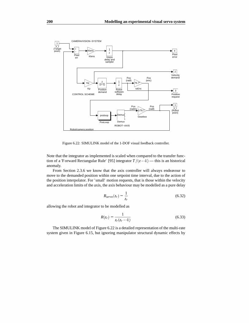
200 Modelling an experimentalvisual servosystem
3
Positionrequest
z
1
Robotsoftware
delay
2
Velocitydemand
1x_r
(Robotposn)
1x_t
(Targetposn)
z(z−1)
Positiondemand
Kp
Kp
1/76.7
Gearbox
76.7*
toEnc
Robot/camera position
CAMERA/VISION−SYSTEM
CONTROL SCHEME
Pos(radl)
Pos(radl)
Pos(radm)
Pos(enc)
Demux
Demux
posloop
PosLoop
ROBOT−AXIS
+−
Pixelerr
Klens
Klens
z
1
Visiondelay andsampler
4
Pixelerror
Figure6.22:SIMULINK modelof the1-DOFvisualfeedbackcontroller.
Notethattheintegratorasimplementedis scaledwhencomparedto thetransferfunc-tion of a 'ForwardRectangularRule' [95] integratorT z 1 — this is anhistoricalanomaly.
From Section2.3.6 we know that the axis controllerwill alwaysendeavour tomove to thedemandedpositionwithin onesetpointtime interval, dueto theactionofthepositioninterpolator. For 'small' motionrequests,thatis thosewithin thevelocityandaccelerationlimits of theaxis,theaxisbehaviour maybemodelledasapuredelay
Rservo zr1zr
(6.32)
allowing therobotandintegratorto bemodelledas
R zr1
zr zr 1(6.33)
TheSIMULINK modelof Figure6.22is adetailedrepresentationof themulti-ratesystemgiven in Figure6.15,but ignoringmanipulatorstructuraldynamiceffectsby

6.4Visual feedbackcontrol 201
T2T1
x0 x2
x1
Figure6.23:Multi-ratesamplingexample,T1 20andT2 14.
assumingthatGstruct s 1. Thismodelis basedon themodelsPOSLOOP, VLOOPandLMOTOR andparametervaluesestablishedin Section2.3.Thestepresponsesofthemeasuredsystemandthemodelareshown togetherin Figure6.26alongwith thatof a single-rateapproximationdevelopedlater. Themodelresponseis boundedby themeasuredearlyandlateresponse,andup to 0.16s is parallelto theearlyresponsebutlaggingby around9ms. This lag is dueto the samplersin the simulationnot beingsynchronizedwith thosein themeasuredsystem.Themodelresponseis slightly moredampedthanthemeasuredresponses.
6.4.4 The effectof multi-rate sampling
Multi-ratesystemsin whichtheratesarenot integrally relatedaredifficult to analyze,andthis topic is generallygivenonly cursorytreatmentin textbooks. In this sectiona ratherpragmaticapproachwill be takento modellingthe multi-ratesamplersasasingleratesamplerplusa timedelay. While nota preciseanalysisit doescapturesthedominantor 'first order' characteristicsof thesystem.
A samplerwith interval T will sampleat timesiT wherei is an integer. An edgeat time t will propagatethrougha singlesamplerat time
tT TceiltT
(6.34)
whereceil x returnsaninteger i suchthat i x. This impliesthatanedgeoccurringat theactualsamplinginstantwill bepropagatedimmediately.
Considertheexampleshown in Figure6.23which comprisestwo cascadedsam-plersoperatingat intervalsof T1 andT2 respectively. An edgeoccurringat time t0propagatesthroughthefirst andsecondsamplersat timest1 andt2 respectively. From(6.34)wemaywrite
t1 T1ceilt0T1
(6.35)
t2 T2ceilt1T2
(6.36)
∆20 t2 t0 (6.37)
∆21 t2 t1 (6.38)

202 Modelling an experimentalvisual servosystem
0 50 100 150 200 2500
5
10
15
t0 (ms)
Del
ay21
(m
s)
0 2 4 6 8 10 120
0.05
0.1
0.15
Delay21 (ms)
P(D
elay
21)
Figure6.24: Analysisof samplingtime delay∆21 for thecasewhereT1 20msandT2 14ms.Topshowsvariationin delayversussamplingtime(meanof 6msshown dashed),while bottomshowsprobabilitydistribution.
where∆20 is the delayof the edgefrom input to output,and∆21 is the delayof theedgethroughthesecondsampler. A numericalsimulationof thedelayfor thevisualservo controlcasewhereT1 20msandT2 14mshasbeenconducted.Figures6.24and 6.25 show ∆21 and ∆20 respectively, along with the correspondingprobabilitydistributionsof thedelays.Bothdelayfunctionsareperiodic,with aperiodof 140ms,the leastcommonmultiple of 14 and 20. The meandelay values,markedon thedelayplots, are ∆20 16ms and ∆21 6ms. However the meandelayis sensitiveto therelative 'phasing'of thesamplers,andfurthersimulationshows that∆21 variesperiodicallybetween6 and8msasphaseshift betweenthesamplersis increased.Themeanof ∆21 over all phaseshiftsis one-halfthesamplerinterval,or 7ms.
Clearly the principal effect of multi-ratesamplingis to introducea small timedelay. Thetwo samplersmaybeapproximatedby a singlesampleranda delayin therange6 to 8msdependingonphasingwhichis unknown6. Assuminga samplerdelayof 7mscombinedwith thealreadyidentifieddelayssuchas20msfor pixel transport,14msservo communicationsand14msrobotmotiondelay, thetotal latency is 55ms.
6Sincethetwo samplingprocessesarecontrolledby separateandunsynchronizedclocksit is likely thatthephasingwill varywith time.

6.4Visual feedbackcontrol 203
0 50 100 150 200 2500
10
20
30
40
t0 (ms)
Del
ay20
(m
s)
0 5 10 15 20 25 300
0.002
0.004
0.006
0.008
0.01
Delay20 (ms)
P(D
elay
20)
Figure6.25: Analysisof samplingtime delay∆20 for thecasewhereT1 20msand T2 14ms. Top shows variation in delay versussamplingtime (meanof16msshown dashed),while bottomshowsprobabilitydistribution.
This is consistentwith earlierestimatesof 58msand60msdelay. Furtherrefinementis possibleby accountingfor furthermulti-rateeffectsbetweenthe14msrobotcontrolprocessandthe980µsdigital servo boardprocess,but thiswill notbepursuedfurther.
6.4.5 A single-ratemodel
To simplify analysisthesystemmaybeapproximatedby asingle-ratemodeloperatingwith a samplinginterval of Tv. As implementedV z andD z alreadyoperateat Tv,but it is necessaryto expresstherobotdynamics,R z , at thissamplinginterval
R zr1
zr zr 1(6.39)
1Tr
1zr
Tr
zr 1(6.40)
1Tr
1zv
Tv
zv 1(6.41)

204 Modelling an experimentalvisual servosystem
wherethe rightmostterm, the integrator, hasbeenchangedfrom the robot sampleinterval to thevisualsampleinterval, andtheunit delayTr hasbeenapproximatedbyTv. Introducingthenotationz zv theopen-looptransferfunctionmaybewrittenas
V z D z R zKlens
zKp
1Tr
1z
Tv
z 1(6.42)
KpKlens
z2 z 1Tv
Tr(6.43)
Theresultingsingle-rateclosed-looptransferfunctionis
xr zxt z
Kz3 z2 K
(6.44)
where
KTv
TrKpKlens (6.45)
The overall delayis Ord denominator Ord numerator, in this casethreesampleperiodsor 60ms. From Figure6.21 it canbeseenthat thesearedueto pixel trans-port,velocitycomputationandservo response.This60msdelayagreeswith previousobservationsof latency andthestepresponseof this model,shown in Figure6.26,isseento beboundedby themeasuredearlyandlateresponses.Thesinglerateresponsestartscloseto the early responseand finishescloserto the late response,showingthat it hascapturedthe'average'characteristicof therealsystem.This modelis alsoslightly moredampedthan the measuredresponses.The model (6.44) is the sameasthat determinedby CorkeandGood[62] for the caseof multi-axis translationalfixation.
Thesingle-rateopen-loopmodel(6.43)canbeusedfor stabilityanalysisaswell asstate-estimatorandcontrollerdesignusingclassicaldigital control theory. Theroot-locusdiagramin Figure6.27shows that for the known gainsetting,K 0 132, thepolesare locatedat z 0 789, 0 528and 0 316. The dominantpole correspondsto a frequency of 1.9Hz which is in goodagreementwith theestimateof 2Hz madeearlier. This pole is very sensitive to changesin loop gain suchasthosecausedbyvariationin targetdistance.Figure6.28shows theBodeplot of thesingleratemodeloverlaidon theexperimentallydeterminedfrequency responsefunctionfrom Section6.4.2.
6.4.6 The effectof camerashutter interval
Section3.3.3discussestheeffect of motionblur in termsof shapedistortionandlag-ging centroidestimate.Figure6.29shows very clearlythatwith anexposureintervalof 20ms the apparentareaof the LED target is increasedduring the high velocity

6.4Visual feedbackcontrol 205
0 0.1 0.2 0.3 0.4 0.5 0.60
0.1
0.2
Time (s)
Res
pons
e (r
adl)
Figure6.26: Comparisonof measuredandsimulatedstepresponse.Measuredearly and late stepresponses(dotted),single-ratemodel (solid), andthe multi-ratemodel(dashed).( f 8mm,Klens 724,andKp 1 3 10 4)
-1 -0.5 0 0.5 1-1
-0.8
-0.6
-0.4
-0.2
0
0.2
0.4
0.6
0.8
1
Real Axis
Imag
Axi
s
Figure6.27: Root-locusof single-ratemodel. Closed-looppolesfor gainKp1 3 10 4 aremarked(Klens 708).

206 Modelling an experimentalvisual servosystem
10-1
100
101
-40
-20
0
Freq (Hz)
Mag
(dB
)
10-1
100
101
-400
-200
0
Freq (Hz)
Pha
se (
deg)
Figure6.28: Bodeplot of single-ratemodelclosed-looptransferfunction(solid)with measuredfrequency response(dotted)overlaid.Notetheconsiderablephaseerrorfor moderatefrequency demands,eg. 1Hz. (Kp 1 3 10 4, Klens 708)
phaseof thefixation motion. Thecamerarotationrateis 1.5radl sandhasincreasedtheapparentareaby afactorof 2.6.Thecircularity,(4.11),alsodropsto 0.76from itsnormalvalueof 1.0asthetarget imagebecomeselongated.Theexperimentalvisualservo systemusessimplecriteria to identify the target region from other regionsinthescene,usuallyon thebasisof areaandcircularity. Thesecriteriamustberelaxedin orderthat thecontrollerdoesnot 'lose sight' of thetargetwhenits apparentshapechangessodramatically.
The othereffect of motionblur is to introducea laggingcentroidestimate.Thiswill alter the dynamicsof the closed-loopsystemby increasingopen-looplatency.Figure6.30shows that the increasedlatency hashadtheexpected'destabilizing'ef-fect, resultingin increasedovershoot.
6.4.7 The effectof target range
Section6.3.2showedthatavisualservoingsystemintroducesatargetdistancedepen-dentgaindueto the lens,which will affect the loop gainandstability of the closed-loop system. Few reportson visual servoing discussthis effect, but muchwork isperformedwith fixedcamera-targetdistances— perhapsdueto focusor depthof field

6.4Visual feedbackcontrol 207
1 1.5 2 2.5 3100
150
200
250
300
350
Time (s)
Are
a (p
ixel
s)
1 1.5 2 2.5 30
0.05
0.1
0.15
0.2
0.25
Time (s)
The
ta (
radl
)
Figure6.29: Measuredeffect of motion blur on apparenttarget areafor 'long'exposureinterval (Te 20ms). The lower plot shows the camerapanangleinresponseto a stepchangein target position; the apparenttarget areaat corre-spondingtimes is shown in the upperplot. During the highest-velocity motionapparentareaof theLED targethasincreasedby a factorof 2.6.
problems.This issueis mentionedby Dzialo andSchalkoff [81] in the control of apan-tilt camerahead.Experimentalresults,for thecaseof translationalfixation,havebeenreportedby CorkeandGood[62]. Pool[206] recognizedthisproblemin thecit-ruspickingapplication,astherobotapproachesthefruit, andusedanultrasonicsensorto measurerangein orderto modify thevisualloop gainduringapproachmotion.
Measuredstepresponsesfor differentcamera-objectdistancesareshown in Fig-ure6.31. Theincreasedloop gainfor low targetrangeresultsin increasedovershoot.In this experiment,with rotationalfixation motion,thedistancedependenceis weak.With translationalfixation this effect is much morepronounced[62]. An adaptivecontrolleror a self-tuningregulatorcouldmaintainthe desireddynamicresponseastarget distancechanged,andthe parametervalueswould bea functionof targetdis-tance.This introducesthepossibilityof determiningobjectdistancefrom closed-loopdynamicsusinga singlecameraandwithoutprior knowledgeof objectsize.

208 Modelling an experimentalvisual servosystem
0 0.1 0.2 0.3 0.4 0.5 0.6 0.7 0.80
0.2
0.4
0.6
0.8
1
1.2
Time (s)
Nor
mal
ized
res
pons
e
Figure6.30: Measuredstepresponsesfor exposureintervals of 2ms, 8ms and20ms. The responsebecomesmore oscillatory as the exposureinterval is in-creased.Conditionsareobjectrange460mmandKp 1 4 10 4.
6.4.8 Comparisonwith joint control schemes
Thevisualservo controllerandtheconventionalaxispositioncontrollerdescribedinSection2.3.6both employa sensorwhich quantizespositioninto unit steps:eitherpixels or encodercounts. For the joint 6 visual servo experimentdescribedin thissection,andignoringcenterof rotationissues,onepixel correspondsto
1pixel1
Klens(6.46)
1αx f
(6.47)
1 6 10 3radl (6.48)
Increasedangularresolutioncanbeobtainedby increasingthefocal length, f , of thelens,but at theexpenseof reducedfield of view. Theangularresolutionof the axispositioncontrolleris determinedby theencoderpitch which is summarizedin Table2.19.
1encoder2π
Nenc
1G6
(6.49)

6.4Visual feedbackcontrol 209
0.1 0.2 0.3 0.4 0.5 0.6 0.7 0.8 0.90
0.2
0.4
0.6
0.8
1
1.2
Time (s)
Nor
mal
ized
res
pons
e
Figure6.31: Measuredstepresponsefor target rangesof 395mm, 470mm and890mm. Theresponsebecomesmoreoscillatoryasthetargetrangeis decreased.
1 6 10 4radl (6.50)
which is oneorderof magnitudebetterthanthe visual servo, andthis axis hasthepoorestencoderresolution.However thevision systemcanachieve somemeasureofsub-pixel precisionaswasdiscussedin Section4.1.3.Comparableaccuracy with theaxis positioncontrollerwould be obtainedif the centroidestimatewereaccurateto0.1pixel. At the3σ confidencelevel
3σXc 0 1 (6.51)
whichfrom (4.53)wouldbeachievedfor acirculartargetwith adiametergreaterthan40pixels.
6.4.9 Summary
This sectionhas investigatedin considerabledetail the operationof a single DOFvisual-feedbackcontrolsystem.With simpleproportionalcontrolit hasbeenpossibleto demonstratestableandhigh-speedmotion control at ratesapproachingthe limitsestablishedin Chapter2. This hasprovidedinsightsinto the interactionbetweenthe

210 Modelling an experimentalvisual servosystem
dynamiccharacteristicsof therobot,its controller, andthevision system.Thevisualservo systemhasbeenmodelledin somedetailandthemodelvalidatedagainstexper-imentalresults. The actualsystemis multi-rate,which complicatesanalysis,but aneffective single-rateapproximationhasbeendevelopedthat compareswell in termsof time andfrequency response.Themulti-ratesamplingprocesswasanalyzedandshown to have a first-ordercharacteristicthatis a constantdelay. A numberof systemcharacteristicsthataffect thedynamicresponsehave beeninvestigatedincludinglenscenterof rotation,exposureinterval andtargetrange.
The experimentalsystemdescribedis well suitedfor this applicationandis ableto minimize delayby overlappingserialpixel transportand imageprocessing.De-spitethis, the dominantdynamiccharacteristicremainsdelaydueto pixel transport,computationandfinite motiontime. Someenhancementsto thearchitecturearepos-sible which will reducedelaybut it cannotbe entirelyeliminated.Thenext chapterwill investigatemoresophisticatedcontrollersandevaluatethemin termsof adefinedperformancemetric.

Chapter 7
Control designandperformance
Most reportedvisual servo systemsdo not performaswell aswould beexpectedordesired. The mostobvious characteristicsareslownessof motion, lag with respectto targetmotion,andoftensignificantjitter or shakiness.All of thesecharacteristicsareindicative of poorly designedcontrolsystems,inappropriatecontrolarchitecturesor both. This chapterfocusseson issuesof controlsystemperformanceanddesign:definingthecontrolsystemsproblem,definingperformancemeasures,andcomparinga numberof differentcontroltechniquesfor challengingtargetmotion.
As shown in thepreviouschaptersmachinevisionhasanumberof significantdis-advantageswhenusedasa feedbacksensor:a relatively low samplerate,significantlatency (oneor moresampleintervals)andcoarsequantization.While thesecharacter-isticspresenta challengefor thedesignof high-performancemotioncontrolsystemsthey arenot insurmountable.
Latency is themostsignificantdynamiccharacteristicandits sources,asdiscussedpreviously, include: transportdelayof pixels from camerato vision system,imageprocessingalgorithms,communicationsbetweenvisionsystemandcontrolcomputer,controlalgorithmsoftware,andcommunicationswith therobot. In fact problemsofdelayin visual servo systemswerefirst notedover 15 yearsago[116]. If the targetmotion is constantthenpredictioncanbe usedto compensatefor latency, but com-binedwith a low samplerateresultsin poordisturbancerejectionandlong reactiontimeto target'maneuvers', thatis,unmodeledmotion.Graspingobjectsonaconveyorbelt [290] or a moving train [7] arehowever idealapplicationsfor prediction.
Franklin[95] suggeststhatthesamplerateof adigital controlsystembebetween4and20timesthedesiredclosed-loopbandwidth.For thecaseof a50Hzvisionsystemthis implies that a closed-loopbandwidthbetween2.5Hz and 12Hz is achievable.
211
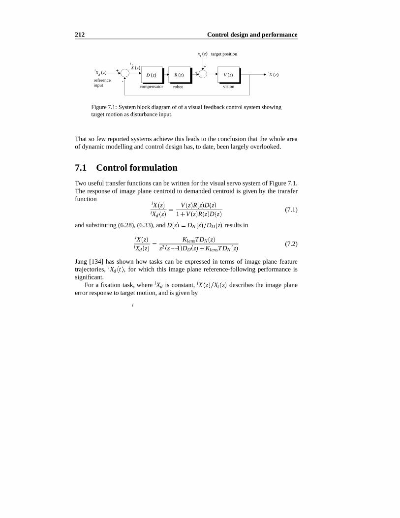
212 Control designand performance
D z( ) V z( )R z( )+
xt z( )
+
-
Xi
dz( ) X
iz( )
compensator robot vision
target position
referenceinput
+Xi
z( )
Figure7.1: Systemblockdiagramof of avisualfeedbackcontrolsystemshowingtargetmotionasdisturbanceinput.
Thatso few reportedsystemsachieve this leadsto theconclusionthat thewholeareaof dynamicmodellingandcontroldesignhas,to date,beenlargelyoverlooked.
7.1 Control formulation
Two usefultransferfunctionscanbewritten for thevisualservo systemof Figure7.1.The responseof imageplanecentroidto demandedcentroidis givenby the transferfunction
iX ziXd z
V z R z D z1 V z R z D z
(7.1)
andsubstituting(6.28),(6.33),andD z DN z DD z resultsin
iX ziXd z
KlensTDN zz2 z 1 DD z KlensTDN z
(7.2)
Jang[134] hasshown how taskscan be expressedin termsof imageplanefeaturetrajectories,iXd t , for which this imageplanereference-following performanceissignificant.
For a fixation task,whereiXd is constant,iX z Xt z describesthe imageplaneerrorresponseto targetmotion,andis givenby
i X zXt z
V z1 V z R z D z
(7.3)
Klensz z 1 DD zz2 z 1 DD z KlensDN z
(7.4)
wherei X iXdiX is theimageplaneerrorandiXd is assumed,for convenience,to
bezero.Themotionof thetarget,xt , canbeconsideredadisturbanceinputandideallythedisturbanceresponse,i X z Xt z , would bezero.However with thepreviouslyidentifieddynamicsit is nonzeroandriseswith frequency. To obtainbettertracking

7.1Control formulation 213
performanceit is necessaryto reduce i X z Xt z over thetargetmotion'sfrequencyrange.
The steady-statevalueof the imageplaneerror for a given target motion,Xt z ,canbefoundby thefinal-valuetheorem
limt ∞
i X t limz 1
z 1 i X z (7.5)
limz 1
z 1V z
1 V z R z D zXt z (7.6)
Usingproportionalcontrolandsubstitutingpreviously identifiedmodelsfor V z andR z thesteady-stateerroris
i X ∞ limz 1
z 1Klensz z 1
z2 z 1 KpKlensXt z (7.7)
whichmaybeevaluatedwith thetargetmotionchosenasoneof
Xt z
zz 1 for a stepinput
Tzz 1 2 for a rampinput
T2
2z z 1z 1 3 for a parabolicinput
(7.8)
For thesteady-statetrackingerror to bezero,thenumeratorof (7.7) mustcancelthe polesat z 1 of Xt z andretaina factor of z 1 . This numeratorcomprisesthepolesof therobotandcompensatortransferfunctions— thelattermaybeselectedto give thedesiredsteady-stateerrorresponseby inclusionof anappropriatenumberof integratorterms,or z 1 factors. The numberof suchopen-loopintegratorsisreferredto as the Type of the systemin classicalcontrol literature. Equation(7.7)hasoneopen-loopintegratorandis thusof Type1 giving zerosteady-stateerrorto astepinput. The additionof an integratorto raisesystemType supportsthe intuitiveargumentof Section6.4whichsuggestedthatthecontrolproblembeconsideredasa'steeringproblem',wheretherobotvelocity, notposition,becontrolled.
A rampinputhoweverwill resultin afinite errorof T Kppixelswhichcanbeseenasthesubstantiallag in Figure7.2. Also notethat thenumeratorof the closed-looptransferfunction (7.4) hasa zeroat z 1 which actsasa differentiator. From (7.4)compensatorpoleswill appearasadditionalclosed-loopzeros.
Commonapproachesto achieving improvedtrackingperformanceare:
1. Increasingtheloopgain,Kp, whichminimizesthemagnitudeof ramp-followingerror. However for the system,(6.44), this is not feasiblewithout additionalcompensationastheroot-locusplot of Figure6.27showed.
2. IncreasingtheTypeof thesystem,by addingopen-loopintegrators.Type1 and2 systemswill have zerosteady-stateerror to a stepandrampdemandrespec-tively.

214 Control designand performance
3. Introducingfeedforwardof thesignalto be tracked.This is a commonlyusedtechniquein machine-toolcontrol and has beendiscussed,for instance,byTomizuka[251]. For the visual servo system,the signal to be trackedis thetarget positionwhich is not directly measurable.It canhowever beestimatedandthis approachis investigatedin Section7.5.
7.2 Performancemetrics
It is currentlydifficult to comparethe temporalperformanceof variousvisual servosystemsdueto thelack of any agreedperformancemeasures.At bestonly qualitativeassessmentscanbemadefrom examiningthetimeaxisscalingof publishedresults(isit trackingat1mm s or 1000mm s?) or videotapepresentations.
Traditionally the performanceof a closed-loopsystemis measuredin termsofbandwidth. While 'high bandwidth' is desirableto reduceerror it can also lead toa systemthat is sensitive to noiseandunmodeleddynamics.However the notionofbandwidthis not straightforwardsinceit implies both magnitude(3dB down) andphase(45 lag) characteristics.Time delayintroducesa linear increasein phasewithfrequency, andtheBodeplot of Figure6.28indicates45 lagoccursat lessthan1Hz.For trackingapplicationsphaseis a particularlymeaningfulperformancemeasure—for instancethecitruspicking robot'strackingspecificationwasin termsof phase.
Othercommonlyusedperformancemetricssuchassettlingtime, overshootandpolynomialsignal following errorsareappropriate.Note thoughthat the feedbacksystemdevelopedin theprevioussectionhasa 'respectable'squarewave responsebutexperimentsshow poorability to follow a sinusoid.Simulatedtrackingof sinusoidalmotion in Figure7.2 shows a robot lag of approximately30 andthe centroiderrorpeakingatover 80pixels.
In this work we chooseto considerthe magnitudeof imageplaneerror, eitherpeak-to-peakor RMS, in order to quantitatively measureperformance.The RMSerrorover thetime interval t1 t2 is givenby
η
t2
t1
iX t iXd t 2dt
t2 t1(7.9)
An image-planeerrormeasureis appropriatesincethefixationtaskitself is definedin termsof imageplaneerror, andis ideallyzero.Imageplaneerroris computedby thecontrollerandcaneasilybe logged,andthis is considerablysimplerthanestimatingclosed-loopbandwidth.
The choiceof appropriatetarget motionwith which to evaluateperformancede-pendsupontheapplication.For instanceif trackinga falling or flying objectit wouldbe appropriateto usea parabolicinput. A sinusoidis particularlychallengingsince

7.3Compensatordesignand evaluation 215
0 0.5 1 1.5 2 2.5 3-0.2
-0.1
0
0.1
0.2
Time (s)
Res
pons
e (r
adl)
0 0.5 1 1.5 2 2.5 3-100
-50
0
50
100
Time (s)
Err
or (
pix)
Figure7.2: Simulatedtrackingperformanceof visualfeedbackcontroller, wherethe target is moving sinusoidallywith a periodof 1.5s (0.67Hz). Note thecon-siderablelagof theresponse(solid) to thedemand(dashed).
it is a non-polynomialwith significantandpersistentaccelerationthatcanbereadilycreatedexperimentallyusinga pendulumor turntable. Sinusoidalexcitation clearlyrevealsphaseerrorwhich is a consequenceof open-looplatency. In theremainderofthis work a fixedfrequency sinusoid
xt t M sin 4 2t (7.10)
will beusedasthestandardtargetmotion. This correspondsto anobjectrotatingonthe laboratoryturntableat its maximumrotationalspeedof 40rpm (0.67rev s). Themagnitude,M, of thetargetmotiondependson therotationalradiusof thetarget,andthe distanceof the camera. Peakangulartarget velocity is 4 2M rad s andcan beselectedto challengetheaxiscapability.
7.3 Compensatordesignand evaluation
7.3.1 Addition of an extra integrator
A controllerwith improved trackingperformancemust incorporateat leastone

216 Control designand performance
-1.5 -1 -0.5 0 0.5 1 1.5-1.5
-1
-0.5
0
0.5
1
1.5
Real Axis
Imag
Axi
s
Figure7.3: Root locusfor visual feedbacksystemwith additionalintegratorandproportionalcontrol.Clearlythesystemis unstablefor any finite loopgain.
additionalintegratorfor Type2 characteristics.Theopen-looptransferfunction(6.43)becomes
KpKlens
z2 z 1 2
KpKlens
z4 2z3 z2 (7.11)
which,without additionalcompensation,is unstablefor any finite loopgainasshownby theroot-locusin Figure7.3.
7.3.2 PID controller
A discretetimePID compensatorcanbewrittenas
D z PTz
z 1I
1 z 1
TD (7.12)
z2 PT IT2 D z PT 2D DTz z 1
(7.13)
whereP, I andD aretheproportional,integral andderivative gainsrespectively, andT thesamplinginterval. Thederivative is computedby meansof a simplefirst-orderdifference.This compensatoraddsa pole at z 1 which increasesthe Type of the

7.3Compensatordesignand evaluation 217
-1 -0.5 0 0.5 1-1
-0.8
-0.6
-0.4
-0.2
0
0.2
0.4
0.6
0.8
1
Real Axis
Imag
Axi
s
Figure 7.4: Root locus for visual feedbacksystemwith PID controller whichplacesthezerosatz 0 3andz 0 9. Theclosed-looppolesmarkedby squaresareusedin thesimulationof Figure7.5.
systemasdesired,andallows arbitraryplacementof the two zerosto shapethe rootlocus.
An exampleroot locusis shown in Figure7.4. Onezero is placedcloseto z1 in order to 'bend' the armsof the root locus inside the unit circle, however it isnot possibleto move thedominantclosed-looppolesso asto achieve a high naturalfrequency. Theclosed-looptransferfunctionis
iX zxt z
KlensTz2 z 1 2
z3 z 1 2T KlensT z2 PT IT2 D z PT 2D D(7.14)
which, sincethe systemType is 2, hasa pair of closed-loopzerosat z 1. Thisdoubledifferentiatorcausessignificantovershootin responseto targetacceleration—notetheinitial transientin Figure7.5. Thecompensatorzeroscouldbeconfiguredasa complex pairbut mustbeplacedcloseto z 1 if they areto 'capture' theopen-loopintegratorpoles,whichwouldotherwiseleave theunit circlerapidly.
In practiceit is foundthatderivativegainmustbelimited,sincethederivativetermintroducesundesirable'roughness'to thecontrol,andthis constrainsthelocationsofthe open-loopzeros. This roughnessis a consequenceof numericallydifferentiat-ing the quantizedandnoisycentroidestimatesfrom the vision system.Astrom and
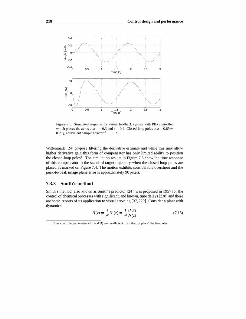
218 Control designand performance
0 0.5 1 1.5 2 2.5 3-0.4
-0.2
0
0.2
0.4
Time (s)
Ang
le (
radl
)
0 0.5 1 1.5 2 2.5 3
-50
0
50
Time (s)
Err
or (
pix)
Figure7.5: Simulatedresponsefor visual feedbacksystemwith PID controllerwhichplacesthezerosat z 0 3 andz 0 9. Closed-looppolesat z 0 850 20j, equivalentdampingfactorζ 0 52.
Wittenmark[24] proposefiltering the derivative estimateandwhile this may allowhigherderivative gain this form of compensatorhasonly limited ability to positionthe closed-looppoles1. Thesimulationresultsin Figure7.5 show the time responseof this compensatorto the standardtarget trajectorywhenthe closed-looppolesareplacedasmarkedon Figure7.4. Themotionexhibits considerableovershootandthepeak-to-peakimageplaneerroris approximately90pixels.
7.3.3 Smith'smethod
Smith's method,alsoknown asSmith's predictor[24], wasproposedin 1957for thecontrolof chemicalprocesseswith significant,andknown,timedelays[238] andtherearesomereportsof its applicationto visualservoing [37,229]. Considera plantwithdynamics
H z1zd
H z1zd
B zA z
(7.15)
1Threecontrollerparameters(P, I andD) areinsufficient to arbitrarily 'place' thefive poles.

7.3Compensatordesignand evaluation 219
whereOrd A Ord B and d is the time delayof the system. A compensator,D z , isdesignedtogivedesiredperformancefor thedelay-freesystemH z . Smith'scontrollaw givestheplantinputas
U D Yd Y D H 1 z d U (7.16)
whichcanbeexpressedasa compensatortransferfunction
D zzdA D
zd A B D B D(7.17)
whichclearlyattemptsto canceltheplantdynamicsA z . Thevisualservo open-loopmodelof (6.43)canbewrittenin theform
H z1z2
Kz 1
1z2H z (7.18)
anda simpleproportionalcompensator, D Kp, usedto controlthedynamicsof thefirst-ordersystemH z . Theresultingcompensatorby (7.17)is
D zz2 z 1 Kp
z2 z 1 KKp z2 1(7.19)
Whensimulatedwith thelinearsingle-ratemodelthecompensatorgivestheexpectedperformanceandthepolecanbepositionedto givearbitrarily fastperformance.How-ever whensimulatedwith the full non-linearmulti-ratemodelsimilar to Figure6.22theeffect of modelerrorsbecameapparent.Theclosed-looppoleof H z couldnolongerbearbitrarily positionedandattemptsto placethe poleat z 0 6 led to poordynamicresponseandinstability. Figure7.6showstheresponsefor thecaseof z 0 6whichshowsa peak-to-peakerrorof nearly70pixels.
Sharkey et al. [229] report experimentalgazecontrol resultsobtainedwith the'Yorick' head. Using accurateknowledgeof actuatorandvision processingdelaysa target positionand velocity predictoris usedto counterthe delayand commandthe positioncontrolledactuators.They suggestthat this scheme“naturally emulatestheSmithRegulator” andblock diagrammanipulationis usedto show thesimilarityof their schemeto thatof Smith,however no quantitativeperformancedatais given.Brown [37] usedsimulationto investigatetheapplicationof Smith'spredictorto gazecontrolby meansof simulationandthusdid nothave problemsdueto plantmodellingerrorencounteredhere.He alsoassumedthatall delaywasin theactuator, not in thesensoror feedbackpath.
7.3.4 Statefeedbackcontroller with integral action
State-feedbackcontrol canbe usedto arbitrarily positionthe closed-looppolesof aplant. For besttrackingperformancethe polesshouldall be placedat the origin in

220 Control designand performance
0 0.5 1 1.5 2 2.5 3
-0.2
-0.1
0
0.1
0.2
0.3
Time (s)
Ang
le (
radl
)
0 0.5 1 1.5 2 2.5 3-40
-20
0
20
40
60
Time (s)
Err
or (
pix)
Figure7.6: Simulationof Smith's predictive controller(7.23)anddetailednon-linearmulti-ratesystemmodel.Simulatedresponse(solid)anddemand(dotted).
order that the closed-loopsystemfunctionsas a puredelay, but this may result inun-realizablecontrolinputsto theplant.
Theconfigurationof plant,stateestimatorandcontrollerareshown in Figure7.7.Theopen-loopsystem,V z R z is representedin state-spaceform as
xk 1 xk uk (7.20)
yk
Cxk (7.21)
The estimatorshown is predictive, andallows one full sampleinterval in which tocomputethe stateestimate,x, and the control input, u. Within the labelledcom-pensatorblock thereis feedbackof the computedplant input to the estimator. Theclosed-loopcompensatorpolesaretheeigenvaluesof
KeC K (7.22)
whereK is thestate-feedbackgain matrix andKe is theestimatorgainmatrix. Theseparationprinciple[95] statesthatthepolesof a closed-loopsystemwith anestima-tor is theunion of thepolesof the estimatorandthecontrolledplant,andthat thesemay be designedindependently. However thereis an additionalconsiderationthatthe compensatoritself mustbestable, andthis constrainstheselectionof plantand

7.3Compensatordesignand evaluation 221
xk 1+
Φxk
∆uk
Ke yk
Cxk
−( )+ +=
K−
State-feedbackcontrol
State estimator
xk z 1− x
k 1+
Computationaldelay
V z( )
R z( )
+xt z( )
-
robot
visiontarget
Xi
z( )
position
D z( )
u˜ k
Figure7.7: Visualfeedbacksystemwith state-feedbackcontrolandestimator.
estimatorpole locations. The requirementof compensatorstability appearsto be amatterof somedebateand is not well coveredin standardtexts. Simpleexamplescanbecontrived in which anunstableplantandanunstablecompensatorresultin astableclosed-loopsystem.However Maciejowski [178] statesthat thereis a “theo-retical justificationfor preferring(open-loop)stablecontrollers— but therearealsopowerful practicalreasonsfor thispreference”.Simulationsshow thatwhile anunsta-blecompensatormaygive perfectlysatisfactoryperformancein a lineardiscrete-timesimulation,a moredetailedsimulationor the introductionof modelerrorcaninduceinstability. This is believedto berelatedto plantnon-linearity, where'internal' signalsbetweenthecompensatorandplantmayresultin saturation,changingtheapparentdy-namicsof theplantandleadingto instability.
Compensatorshave beendesignedfor thesingle-rateapproximation(6.43)usingpoleplacementandLQG designprocedures.Astrom andWittenmark[24] describeaprocedurefor designingpoleplacementcompensatorsfor SISOsystemsbasedonstatefeedbackandstateestimation.Considerableexperimentationwasrequiredto chooseclosed-loopand estimatorpolesthat result in a stablecompensator. Franklin [95]suggeststhat theestimatorpolesbe4 timesfasterthanthedesiredclosed-looppoles.Theupperlimit onestimatorresponseis basedonnoiserejectionandmodellingerrors.To reducethedegreesof freedomin thecontrol/estimatordesignprocesstheestimatorpoleswereplacedatz 0 0 0givingadead-beatresponse.In detailedsimulationandexperimentthis hasgivensatisfactoryperformance.Introducinganadditionalopen-loop integrator, andplacingtheclosed-looppolesat z 0 6 0 4 j 0 4 resultsin thecompensator
D zz2 7 01z 5 65
z3 0 6z2 0 4z 0 8(7.23)

222 Control designand performance
-1 -0.5 0 0.5 1-1
-0.8
-0.6
-0.4
-0.2
0
0.2
0.4
0.6
0.8
1
Real Axis
Imag
Axi
s
Figure7.8: Root locusfor pole-placementcontroller. Closed-looppolesat z0 6 0 4 j andz 0 4. Notethatapair of polesandzeroshavebeencancelledattheorigin.
7 01z2 z 0 806
z 1 z 0 2 0 872j(7.24)
The root-locusdiagramin Figure7.8 shows that the compensatorhasintroducedacomplex polepair neartheunit circle andhasbeenableto achieve fasterclosed-looppolesthanthePID compensatorof Figure7.4.Figure7.9showsthesimulatedclosed-loop responsefor the standardtarget motion for both the single-ratemodelandthedetailedSIMULINK model. Thesimulationresultsaresimilar but themoredetailedmodelis somewhat rougherdueto the multi-rateeffects. The peak-to-peakerror inpixel spaceis approximately28pixels.
Clearlythetrackingperformanceis greatlyimprovedcomparedto simplepropor-tionalcontrolbut anumberof characteristicsof theresponsedeserve comment:
Theerror is greatestat thepeaksof thesinusoid,which correspondto greatestacceleration.TheType2 controllerhaszeroerrorfollowing a constantvelocitytarget(which theslopesof thesinusoidapproximate),but will have finite errorfor anacceleratingtarget.
Thereis considerabledelayat t 0 beforetherobotcommencesmoving, due

7.3Compensatordesignand evaluation 223
0 0.5 1 1.5 2 2.5 3-200
-100
0
100
200
Time (s)
Pos
(pi
xels
)
0 0.5 1 1.5 2 2.5 3-20
0
20
40
Time (s)
Err
or (
pixe
ls)
Discrete-timelinearsingle-ratesimulation.
0 0.5 1 1.5 2 2.5 3
-0.2
-0.1
0
0.1
0.2
0.3
Time (s)
Ang
le (
radl
)
0 0.5 1 1.5 2 2.5 3-20
0
20
40
Time (s)
Err
or (
pix)
Non-linearmulti-ratesimulation.
Figure7.9: Simulationof pole-placementfixation controller(7.23). Simulatedresponse(solid)anddemand(dotted).Closed-looppolesat z 0 6 0 4 j 0 4.

224 Control designand performance
0 2 4 6 8 10-4
-2
0
2
4
Time (s)
Imag
e pl
ane
erro
r (p
ixel
s)
0 2 4 6 8 10-0.4
-0.2
0
0.2
0.4
Time (s)
Axi
s ve
loci
ty (
radl
/s)
Figure7.10: Experimentalresultswith pole-placementcompensator. Note thatthetargetfrequency in thisexperimentis only 0.5Hz, lessthanthestandardtargetmotionfrequency. Closed-looppolesatz 0 6 0 4 j 0 4.
to delayin thevisionsystemandcontroller.
Onceagainthis is a Type2 systemandtheclosed-loopresponsewill includeadoubledifferentiator. This effect is evident in the initial transientshown in thesimulatedclosed-loopresponseof Figure7.9.
Experimentalresultsgiven in Figure7.10, for a peakaxis velocity of 0.3radl sandtargetfrequency of approximately0.5Hz,show apeak-to-peakpixel errorof only6pixels. This correspondsvery closelyto simulationresultsfor the sameamplitudetargetmotion,but somelow-amplitudeoscillationataround10Hzcanbeobserved.Inpracticethecompensatorwas' temperamental'anddifficult to initiate. For moderateinitial error the two integratorswind up andsaturatethe axis which leadsto ratherviolent oscillation. It wasfound bestto switch to the pole-placementcompensatorfrom proportionalcontrol oncefixation hadbeenachieved. Table7.1 comparesthesimulatedRMSpixel errorvalueof themodelfor thestandardsinusoidalexcitationatvariousamplitudes.TheRMS errorscalesalmostlinearly with amplitudein thefirstthreerows, but in the lastcaseactuatorsaturationhasoccurredandthepixel error ismuchhigher. High trackingperformanceis achievedbut with a lossof robustnesstoplantsaturationandsomedifficulty in startup.

7.3Compensatordesignand evaluation 225
θpk (radl) θpk radl s RMSpixel error
0.23 0.97 11.10.40 1.70 21.20.45 1.89 24.70.50 2.1 2100
Table7.1: SimulatedRMSpixel errorfor thepole-placementcontrollerasafunc-tionof targetpeakvelocity. SimulatedusingaSIMULINK modelovertheinterval0 to 3s,andincludingtheinitial transient.Notethevery largeerrorin thelastrow— thesystemperformsverybadlyonceactuatorsaturationoccurs.
Designof astateestimatorandstatefeedbackcontrollerusingthelinearquadraticGaussian(LQG) approachhasalsobeeninvestigated,but is complicatedby thestatetransitionmatrix, , beingsingularsincethedelaystatesintroducezeroeigenvalues2.ThecommonLQG designapproaches,implementedby MATLAB toolboxfunctions,arebasedon eigenvectordecompositionandfail for thecaseof a singularstatetran-sition matrix. Instead,therecurrencerelationshipderivedby Kalman[142] from dy-namicprogramming
Mk 1 Q KkRKk Kk Mk Kk (7.25)
Kk 1 R Mk1 Mk (7.26)
wasusedto computethesteady-statevalueof thestatefeedbackgainmatrixgiventhestateandinput weightingmatricesQ andR respectively. This methodis numericallylesssoundthanotherapproachesbut givessatisfactoryresultsfor thelow ordersystemin thiscase.
As in thepreviouscasestableestimatorandclosed-looppolesdo not necessarilyresult in a stablecompensator. The designprocedurerequiresadjustmentof the el-ementsof two weightingmatricesfor eachof the controllerandestimator, resultingin a high-dimensionalitydesignspace.Stableplantsandestimatorscouldbereadilyachievedfor aType1 system,but not for thedesiredcasewith anadditionalintegrator(Type2).
7.3.5 Summary
Theimageplaneerrorsfor eachcompensator, to thesamesinusoidallymoving target,arecomparedin Figure7.11. Thesimulationsarebasedon detailedmulti-ratenon-linearmodelsof thepositionandvelocity loopsof theUnimatePumaservo system.
2Thedeterminantof a matrix is theproductof its eigenvalues,det A ∏i ei , so anyzeroeigenvalueresultsin asingularmatrix.

226 Control designand performance
feedforward
poleplace
PID
proportional
0 0.5 1 1.5 2 2.5 3 3.5 4 4.5 5−300
−200
−100
0
100
200
300
Time (s)
Err
or (
pix)
Figure 7.11: Comparisonof image plane error for various visual feed-back compensatorsfrom above. Target motion in all casesis the sinusoid0 5sin 4 2t radm s.
The simple proportionalfeedbackcontroller, while demonstratingan adequatestepresponse,haspoor trackingperformanceand this may be improved by meansof a moresophisticatedcompensator.
The compensatordesignapproachhasfollowedclassicallinear principlesof in-creasingsystemTypeandpositioningtheclosed-looppolesby meansof PID or pole-placementcontrol. Thesystem's Type is importantto thesteady-statetrackingerrorandat leastType 2 is necessaryto adequatelytrack sinusoidalor parabolicmotion.However in theshortterm,trackingperformanceis dependentontheclosed-looppolelocations. This is illustratedquite clearly in Figure 7.12 which shows the Type 2systemfrom above following a target moving with triangularpositionprofile. Idealtrackingbehaviour is observed during the regionsof constantvelocity demand,butthesettlingtime aftereachpeakis around300ms,the time constantof thedominantclosed-looppoles. Theseclosed-looppolescannotbe madearbitrarily fast andareconstrainedby the practicalrequirementfor compensatorstability. Linear discrete-time simulationsindicateno difficulty with anunstablecompensator, but non-linearsimulationsshow that theclosed-loopsystemwill beunstable.This is believedto bedueto non-linearitiesin theplantwhichchangetheapparentdynamicsat saturation.
The additionof integrators,while raisingthe systemType,placesstringentcon-

7.4Axis control modesfor visual servoing 227
0 0.5 1 1.5 2 2.5 3-200
-100
0
100
200
Time (s)
Pos
ition
(pi
x)
0 0.5 1 1.5 2 2.5 3-50
0
50
Time (s)
Err
or (
pix)
Figure7.12:Simulationof pole-placementfixationcontroller(7.23)for triangulartargetmotion.Closed-looppolesatz 0 6 0 4 j 0 4.
straintsonclosed-loopandestimatorpolelocations.Closeagreementhasbeenshown betweenexperimentaland simulationresults
usingbothlinearsingle-rateandnon-linearmulti-ratemodels.Thecontrollerdesignshave beenbasedon thesingle-ratemodel(6.44)andthesuccessof thecompensatorsis animplicit endorsementof thatmodel'saccuracy.
7.4 Axis control modesfor visual servoing
All theexperimentssofardescribed,andthoseof many others,for example[8,91,134,197,231,270],arebasedonanapproachin whichthevisualservo isbuilt 'on topof' anunderlyingposition-controlledmanipulator. This is probablyfor thepragmaticreasonthatmostrobotcontrollerspresenttheabstractionof a robotasa position-controlleddevice. Therearesomereportsof theuseof axis velocity control [58,63,111,206],andWeiss[273] proposedvisualcontrolof actuatortorque.
This sectionwill comparetheperformanceof visualservo systemsbasedaroundposition,velocity andtorque-controlledactuators.Motion of a robot manipulatoriscausedby actuatorsexerting torquesat the joints. In conventionalrobotapplicationswhereend-pointpositioncontrol is required,it is commonto establishanabstraction

228 Control designand performance
wherebythe axes are capableof following the joint angledemandsof a trajectorygenerator. Suchanabstractionis achievedby closinga position-control loop aroundtheactuator.
Many robotsemploya 'classic' nestedcontrol structurewhich is typical of ma-chine tool controllers,commonlycomprisingcurrent,velocity andposition-controlloops.Thenestedloop,or hierarchical,controlstructurehasa numberof advantagesincluding:
1. The effective dynamicspresentedby theclosed-loopsystemto the outer looparesimplifiedandideally independentof parameteruncertainty.
2. Thedynamicspresentedaregenerallyfirst or secondorder, allowing thedesignto be carriedout in a seriesof relatively simplestepsusingclassicalcontroltechniques.This issueis not asimportantasit oncewas,given the power ofmoderncontrol designtools andavailablecomputationalhardwarefor imple-mentingmoderncontrolalgorithms.
ThePuma's velocity loop providesa goodexampleof reducingparameteruncer-tainty. This loop is closedaroundtheactuatordynamicsfor which thepoleandDCgainarefunctionsof inertiaandfriction. Thehigh-gainvelocity loop minimizestheeffect of variationin theseparameterson the closed-loopdynamics.An alternativeapproach,now feasibledueto low-costhigh-performancecomputing,is to feedfor-wardtorqueto compensatefor changinginertiaandfriction. Theseestimatesmaybederivedfrom afixedparametermodelidentifiedexperimentallyor from onlineidenti-ficationandadaptation.
The next sectionswill examinethedynamicsof a visualservo systemwheretheactuatoris treatedat variouslevels of abstraction:asa torque,velocity or positionsource.Thenotationis shown in Figure7.13,andit will beassumedthat themulti-rateeffectsandcommunicationslatenciesof theearliersystemhave beeneliminatedby optimizationof thecontrolarchitecture.Thedynamicswill all beformulatedat thevisualsamplinginterval,T 20ms. Themodelsof actuatordynamicsusedarethoseestablishedearlier in Chapter2, andthe vision systemis modelledasa singletimestepdelayV z Klens z.
7.4.1 Torquecontrol
The actionof the power amplifier's currentloop allows motor current(proportionalto motor torque)to becommandeddirectly. From(2.65)the transferfunctionof theactuatoris
R sΘm sU s
1s
KiKm
Jms Bm(7.27)
whereθm is the shaft angle,u t the motor currentdemandvid, Jm the inertia, Bm
theviscousfriction, Ki theamplifier transconductanceandKm themotor torquecon-

7.4Axis control modesfor visual servoing 229
V z( )R z( ) -
θt
+
u t( ) y t( )
robot vision
target position
θm
Figure7.13:Block diagramof generalizedactuatorandvisionsystem.
stant.Thediscrete-timetransferfunctionis obtainedby introducinga zero-orderholdnetworkandtakingtheZ-transform
Θm zU z
Z1 e sT
s1s
KiKm
Js B(7.28)
Usingthemodelof (2.64)thediscrete-timedynamicsare
Θm zU z
0 126z 0 81
z 1 z 0 534(7.29)
wherethe zerois dueto thezero-orderhold andsampler. Adding thevision systemdelayresultsin theopen-looptransferfunction
i X zU z
0 126Klensz 0 81
z z 1 z 0 534(7.30)
anda root-locusplot is shown in Figure7.14. Without any compensationtheclosed-looppolesarelimited to having avery low naturalfrequency.
7.4.2 Velocity control
Thetransferfunctionof theUnimateanalogvelocity loop is
R sΘm sU s
1s
Kv
s pv(7.31)
whereu t is thevelocitydemandinputωd andKv thegainof thevelocityloopwhichhasa poleat s pv. Usingthemodel(2.78)anda similar procedureto above, theopen-looptransferfunctionis
i X zU z
0 162Klensz 0 39
z z 1 z 0 051(7.32)
The velocity-looppole is very fast with respectto the samplinginterval andis thusvery closeto theorigin on the Z-plane. Figure7.15shows a root-locusplot for thissystem.

230 Control designand performance
-1 -0.5 0 0.5 1-1
-0.8
-0.6
-0.4
-0.2
0
0.2
0.4
0.6
0.8
1
Real Axis
Imag
Axi
s
Figure7.14:Rootlocusfor visualservo with actuatortorquecontroller.
-1 -0.5 0 0.5 1-1
-0.8
-0.6
-0.4
-0.2
0
0.2
0.4
0.6
0.8
1
Real Axis
Imag
Axi
s
Figure7.15:Rootlocusfor visualservo with actuatorvelocity controller.

7.4Axis control modesfor visual servoing 231
7.4.3 Position control
As explainedin Section2.3.6thepositionloop containsaninterpolatorwhichmovesthejoint to thedesiredvalueover thesetpointinterval of thetrajectorygenerator, Ttg,provided velocity andaccelerationlimits arenot exceeded.Generallythe position-loop sampleinterval is an order of magnitudesmaller than Ttg providing accuratepositioncontrol andgooddisturbancerejection. In a discrete-timesystemwith thesamesamplinginterval, thatis T Ttg, thepositioncontrolleractsasaunit delay, andthediscrete-timedynamicsaresimply
Θm zU z
1z
(7.33)
whereu t is thepositiondemandinputto theposition-controlloop. After introducingthevisionsystemdelay, theopen-looptransferfunctionis
i X zU z
Klens
z2 (7.34)
andFigure7.16showsa root-locusplot for thissystem.
7.4.4 Discussion
All controlmodesresultin abroadlysimilardiscrete-timetransferfunction.In partic-ular:
1. All root-loci have a pole-zeroexcessof two, thusthesystemswill becomeun-stableasgainis increased.
2. All have atransmissiondelay, Ord denom Ord numer, of 2 sampletimes.
3. The previous model(6.44) had3 polesanda 3 sampletime delaydueto thedoublehandlingof setpointdataandthemulti-ratecontrol.
4. Both torque-andvelocity-controlmodeshave oneopen-looppoleat z 1 giv-ing Type 1 characteristics,that is, zerosteady-stateerror to a stepinput. Theposition-controlmoderesultsin aType0 system.
Therobot'stime responseto a unit steptargetmotionis shown in Figure7.18fora simpleproportionalcontrollerwith thegainchosento achieve a dampingfactorof0 7. Thecontrollerbasedona position-modeaxishasa largesteady-stateerrorsinceit is only of Type 0. The velocity-modeaxis control resultsin a significantlyfasterstepresponsethanthatfor torque-mode.
If anintegratoris addedto theposition-modecontrollerthentheresponsebecomessimilar to, but slightly fasterthan, the velocity modecontrollerasshown in Figure
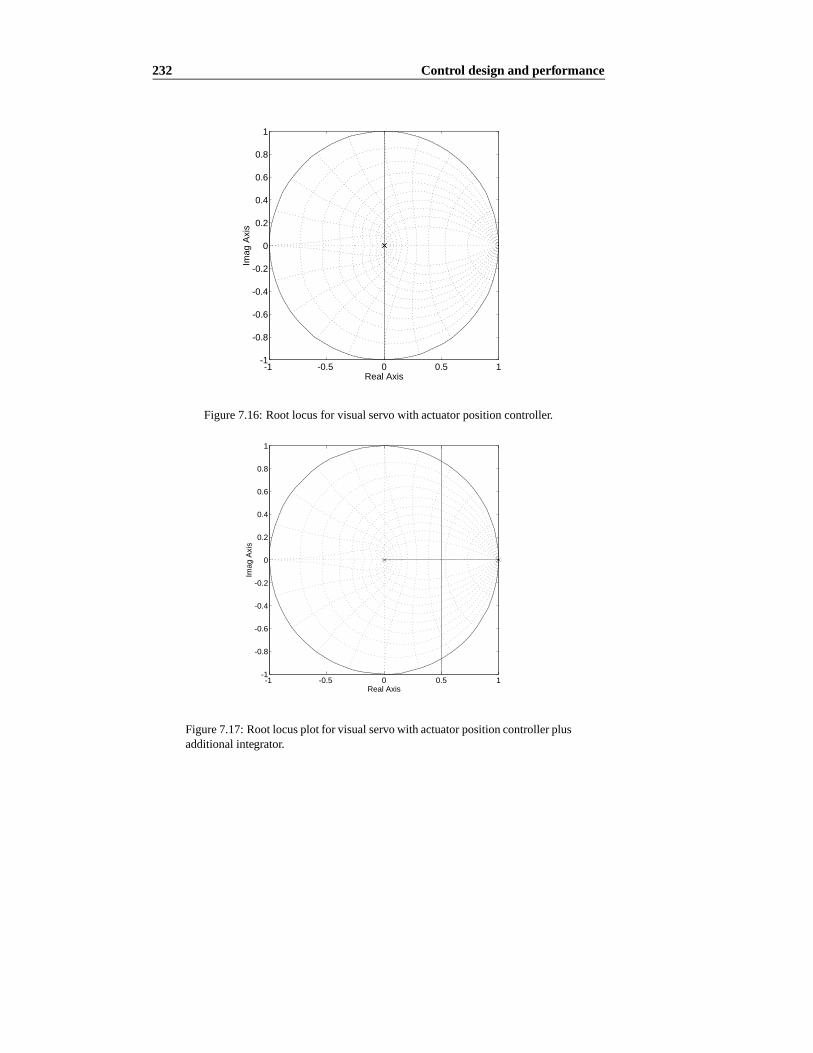
232 Control designand performance
-1 -0.5 0 0.5 1-1
-0.8
-0.6
-0.4
-0.2
0
0.2
0.4
0.6
0.8
1
Real Axis
Imag
Axi
s
Figure7.16:Rootlocusfor visualservo with actuatorpositioncontroller.
-1 -0.5 0 0.5 1-1
-0.8
-0.6
-0.4
-0.2
0
0.2
0.4
0.6
0.8
1
Real Axis
Imag
Axi
s
Figure7.17:Rootlocusplot for visualservowith actuatorpositioncontrollerplusadditionalintegrator.

7.4Axis control modesfor visual servoing 233
0 5 10 15 20 25 300
0.2
0.4
0.6
0.8
1
1.2
Time step
Rob
ot r
espo
nse
Torque
Velocity
Position
Position+integrator
Figure7.18: Simulationof time responsesto targetstepmotion for visual servosystemsbasedontorque,velocityandposition-controlledaxes.Proportionalcon-trol with gainselectedto achieveadampingfactorof 0 7.
7.18. The root locusof this system,Figure7.17, is alsosimilar to that for velocitymodecontrol. The integratorhasturnedtheposition-modecontrollerinto an 'ideal'velocity source,just as usedin the experimentalsystem. From a control systemsperspective however therearesomesubtledifferencesbetweena velocity-controlledaxisandaposition-controlledaxisplusintegrator. In particulartheinnerpositionloopwill generallybe very ' tight', that is high-gain,in orderto minimize positionerror.For anidealrobotthis is nota problem,but it will exacerbateresonanceproblemsdueto structuraland/ordrive compliance. It hasbeenshown [213] that for the caseofsignificantstructuralcomplianceit is preferableto usea 'soft' velocity loop in orderto increasesystemdamping.
7.4.5 Non-linear simulation and modelerror
The above analysisis basedon simple linear modelswhich can maskmany 'real-world' effectssuchasnon-linearityandparametervariation. To investigatethis, for

234 Control designand performance
eachsystemapole-placementcompensator[24] wasdesignedto placetheclosed-looppolesatz 0 6 0 4 j 0 4 0, andraisethesystem'sTypeto 2. Performancewasthensimulatedusingadetailednon-linearmulti-ratesimulationmodelof theaxisdynamicsincludingsaturation,Coulombicandstaticfriction.
For axispositionandvelocity controlmodestheresultsweresimilar to thoseforthe linear simulationcase. However the torque-modecontrollerdid not behave asexpected— the discrete-timenon-linearsimulation,usingmotor modelLMOTOR,resultedin very lightly dampedoscillatoryresponses.This wasfoundto bedueto acombinationof non-linearfriction, integral actionandtherelatively low samplerate.Theunmodeleddynamics,particularlystick/slip friction, arecomplex andhave timeconstantsthatareshorterthanthevisual sampleinterval. It is a 'rule of thumb' thatthe samplerate shouldbe 4 to 20 times the naturalfrequency of the modesto becontrolled.Armstrong[22] commentson oscillationat low velocity dueto theinter-actionof stick/slipfriction with integralcontrol.Anothercauseof poorperformanceisthatthecompensatoris lineartime-invariant(LTI) basedon theassumptionof anLTIplant. However linearizationof the friction model,(2.68), shows that pole locationhasa strongdependenceon shaftspeed,asdoesplantgain. Improved torque-modecontrol would requireoneor moreof the following: a highersamplerate, frictionmeasurementandfeedforward,adaptive,or robustcontrol.
A morestraightforwardoption is theuseof axisvelocity control. Velocity feed-backis effective in linearizingtheaxisdynamicsandminimizing theeffect of param-etervariation. Stablecompensatorsweredesignedandsimulatedfor velocity modecontrolwith Type2 behaviour. Table7.2showstheRMSpixel errorfor thesamesim-ulation run with variationsin motor parameterandvelocity-loopgain settings.TheRMS pixel error is aroundhalf thatof pole-placementcontroller, (7.23),basedon amulti-rateposition-control loopfor thesamemotionamplitude.Interestingly, thesys-tem wasrobust to significantvariationin dynamicparametersandbecameunstableonly whenthevelocity-loopgainwasreduced,weakeningits ability to maskparame-tervariation.
7.4.6 Summary
Theconclusionsfrom thissectioncanbesummarizedasfollows:
1. Control of actuatortorqueusingonly the vision sensorleadsto poor perfor-mancedueto thelow samplerateandnon-linearaxisdynamics.Compensatorsdesignedto increaseperformanceand raisesystemType arenot robust withrespectto theaforementionedeffects.
2. Closinga velocity looparoundtheactuatorlinearizestheaxisandconsiderablyreducestheuncertaintyin axisparameters.
3. Velocityandpositionmodecontrolcanbeusedto achieve satisfactorytracking.

7.5Visual feedforward control 235
Parameter Value Change RMSpixel error
J 41 3 10 6 +25% 6.03J 24 8 10 6 -25% 5.44Kτ 66 8 10 3 +25% 5.42Kτ 40 1 10 3 -25% 6.15Kvel 0 165 -25% unstableKvel 0 275 +25% 6.58
Table7.2: Effect of parametervariationon velocity modecontrol. Simulationsare over 3s with target motion of θt t 0 2sin 4 2t radl, and the LMOTORmotormodelfor joint 6. Compensatordesignedto placetheclosed-looppolesatz 0 6 0 4 j 0 4 0.
4. Position-modecontrol requiresadditionalcomplexity at theaxis control level,for nosignificantperformanceimprovementundervisualservoing.
5. Particularimplementationsof axispositioncontrollersmayintroduceadditionalsamplerateswhichwill degradetheoverall closed-loopperformance.
The approachesreportedin the literatureare interestingwhenconsideredin thelight of theseobservations.Most reportshave closedthevisualpositionloop aroundanaxispositionloopwhichgenerallyoperatesat ahighsamplerate(sampleintervalsof the orderof a few milliseconds). Thereare fewer reportson the useof a visualpositionlooparoundanaxisvelocityloop. Pool[206] usedahydraulicactuatorwhichis a'natural' velocitysource,albeitwith someseverestictioneffects.Hashimoto[111]implementedadigital velocity loopon theaxesof aPumarobotasdid Corke[58,63].Weiss[273] proposedvisual control of actuatortorque,but even with ideal actuatormodelsfoundthatsampleintervalsaslow as3mswererequired.
Earlier it wassuggestedthatvisual fixation shouldbeviewedasa steeringprob-lem, continuouslychangingtherobotvelocity soasto move towardthe goal. Com-binedwith theconsiderationsabove this suggeststhataxisvelocity control is appro-priateto usein a visualservo system.
7.5 Visual feedforward control
Theprevioussectionshave discussedtheuseof visualfeedbackcontrolandexploredthe limits to trackingperformance.Feedbackcontrol involvesmanipulationof theclosed-looppolesandit hasbeenshown thattherearestrongconstraintsontheplace-mentof thosepoles.Anotherdegreeof controllerdesignfreedomis affordedby ma-nipulatingthezerosof theclosed-loopsystem,andthis is achievedby theintroduction

236 Control designand performance
D z( )
V z( )
R z( )
+xt z( )-
compensatorrobot
visiontarget
Xi
z( )
position
DF z( )
feedforward
+
+
Figure7.19:Block diagramof visualservo with feedbackandfeedforwardcompensation.
of a feedforwardterm,DF z , asshown in Figure7.19.Theclosed-looptransferfunc-tion becomes
i Xxt
V z 1 R z DF z1 V z R z D z
(7.35)
whichhasthesamedenominatoras(7.4)but anextra factorin thenumerator. Clearlyif DF z R 1 z thetrackingerrorwouldbezero,but sucha controlstrategy is notrealizablesinceit requires(possiblyfuture) knowledgeof the target positionwhichis not directly measurable.However this informationmay beestimatedasshown inFigure7.20.
Interestinglythe term visual servoinghaslargely replacedthe older term visualfeedback, eventhoughalmostall reportedvisualservo systemsarebasedon feedbackcontrol. The remainderof this sectionintroducesa 2-DOFvisualfixation controllerusing camerapan and tilt motion. Following the conclusionsabove, axis velocityratherthanpositionwill becontrolled.Thevelocity demandwill compriseestimatedtargetvelocity feedforwardandimageplaneerror feedback.A block diagramof thecontroller, usingthenotationdevelopedin thischapter, is shown in Figure7.21.
Thecameramountingarrangementdescribedin Section6.3.1allows camerapanandtilt to beindependentlyactuatedby wrist joints6 and5 respectively. The2-DOFfixation problemis thusconsideredas two independent1-DOF fixation controllers.For simplicity thefollowing discussionwill befor the1-DOFcasebut is readilyap-plied to the2-DOFfixation controller.

7.5Visual feedforward control 237
D z( )
V z( )
R z( )
+xt z( )-
compensatorrobot
vision
targetX
i
z( )
position
DF z( )
feedforward
+
+
E z( )
estimator
xt
Figure7.20:Block diagramof visualservo with feedbackandestimatedfeedfor-wardcompensation.
7.5.1 High-performanceaxis velocity control
Theexperimentsdescribedsofar haveusedtheartificeof anintegratorto implementavelocity-controlledaxis.Thissectioninvestigatestwo approachesto directaxisveloc-ity control. Suchcontroleliminatestwo levelsof complexity presentin theprevioussystem:theintegratorandthepositionloop.
7.5.1.1 Directaccessto Unimate velocity loop
Modificationsweremadeto thefirmwareontheUNIMATEdigital servo cardto allowthehostto directly commandtheanalogvelocity loop describedin Section2.3.5.Asshown in Figure7.22this is a simplevariationof theposition-controlmode,but withthe velocity demandbeingsetby the host,not the setpointinterpolatorandpositionloop. Fromthe hostcomputer's perspective this wasimplementedasa new setpointcommandmode,in additionto theexisting positionandcurrentmodes.A previouslyunusedcommandcodewasusedfor thispurpose.
This modificationallows 'immediate' settingof joint velocityat thevideosamplerate. However the inherentvelocity limit of the velocity loop (seeSection2.3.6) isstill a limiting factorandthe analogloopswerefound to have considerablevelocity

238 Control designand performance
20ms
xrx.d
+
Xi
d
Xi
-
Xi
1
z
D z( )
V z( )
R z( )
+xt z( )-
compensatorrobot
vision
targetposition
E z( )
velocity
+
+
P z( )
target
xtx.t
positionestimator
estimator
Figure7.21: Block diagramof velocity feedforwardandfeedbackcontrolstruc-tureasimplemented.P z estimatestargetbearingfrom (7.43).
Velocityloop
Cur.loop
Digitaltacho
VΩd
Ωm
VIm
VId
DACPositionloop
Counter
ed
em
S1
VDAC M
RS
ImPoweramp
Encoder
S2S2
Figure7.22: Block diagramof Unimationservo in velocity-controlmode.Com-paredwith Figure2.22thedigital positionloop hasbeenbypassedby meansofswitchS1.

7.5Visual feedforward control 239
+ Θl1
s
KiKm
Jms B+m
Kv
ΩmVId
motor+
3z2 4z− 1+
2Tz2
KDAC KG6z 0.85−
z 1−
Ωl
Ωl
PIcompensator
velocity estimator
Ωd
Figure7.23:Block diagramof digital axis-velocity loop for joint 6. Thesamplerateis 50Hz.
offset.
7.5.1.2 Digital axis velocity loop
To overcomethe deficienciesin the Unimateanalogvelocity loop a digital velocityloop hasbeenimplementedwhich commandsmotorcurrentdirectly, andoperatesatthe 50Hz visual samplerate. The overall structure,for joint 6, is shown in Figure7.23.
A key part of the control structureis the estimationof axis velocity from motorshaftanglemeasurements.Thereis considerableliteratureon this topic, particularlyfor the casewherea discretepositionsensor, suchasa shaftangleencoder, is used[30,38,155]. Thetwo majorapproachesare:
1. Countthenumberof encoderpulsesoccurringin afixedtimeinterval, typicallythesampleinterval.
2. Measuretheelapsedtimerequiredfor a givennumberof encoderpulses.
The first approachis easily implementedsincemostaxis controllersprovide an en-codercounter, for axis positionmeasurement,which canbe readperiodically. Thediscretepositionsensorresultsin velocityquantizationof
∆ω∆θT
(7.36)
where∆θ is thepositionquantizationlevel. Velocity resolutioncanbeimprovedby ahigherresolutionpositionsensor, or a longersamplinginterval.
Brown et al. [38] comparea numberof approachesto velocity estimation.Theyconcludethatat high speed,morethan100 countspersamplinginterval, estimatorsbasedon backwarddifferenceexpansionsgive the bestresult. At low speed,tech-niquesbasedon leastsquaresfit areappropriate.The motor shaftvelocitiescorre-spondingto the 100 count limit arecomputedandcomparedwith maximummotor

240 Control designand performance
Joint Counts/rev Critical vel. Percentof(radm/s) maximum
1 1000 5.0 4%2 800 6.3 3.8%3 1000 5.0 3.9%4 1000 5.0 1.2%5 1000 5.0 1.4%6 500 10.0 2.3%
Table7.3: Critical velocitiesfor Puma560velocity estimatorsexpressedasan-gular rateandfractionof maximumaxisrate. Thesecorrespondto 100encoderpulsesper sampleinterval (in this case20ms). Maximum joint velocitiesaretakenfrom Table2.21.
speedfor thePuma560in Table7.3— it is clearthatthebackwarddifferenceestima-tor is appropriatefor themajority of theaxisvelocity range.Belanger[30] comparesfixed-gainKalmanfilters with first-orderfinite differenceexpressionsandconcludesthat the Kalmanfilter is advantageousat short sampleintervals. The Kalmanfilteris anoptimal leastsquaresestimator, andthis resultagreeswith Brown et al. In thisapplicationhowever a Kalmanfilter will be sub-optimal,sincethe axis accelerationis not a zero-meanGaussiansignal. A velocity estimatorcould makeuseof addi-tional informationsuchastheaxisdynamicmodelandcontrolinput. Suchestimators,combinedwith controllers,have beendescribedby Erlic [86] andDeWit [44].
Surprisinglymany papersthat discussexperimentalimplementationof model-basedcontrol makeno mentionof the techniquesusedto estimatemotor velocity,yet from (2.84)and(2.86)it is clearthatknowledgeof motorvelocity is required.Inthis work a second-order, or 3-point,velocity estimator
ˆθi3θi 4θi 1 θi 2
2T(7.37)
is usedwhichcanbederivedfrom thederivativeof a parabolathatfits thecurrentandtwo previouspositionpoints.Thediscrete-timetransferfunctionof this differentiatoris
Ω zΘ z
32T
z 13 z 1
z2 (7.38)
andits frequency responseis shown in Figure7.24.Up to 10Hz theresponsecloselyapproximatesthatof anidealdifferentiator.
Motor current,setvia theUnimatearminterface,is proportionalto velocity errorwith aPI compensatorto giveaclosed-loopDC gainof unity. A detailedSIMULINKmodel,Figure7.25,wasdevelopedandusedto determinesuitablevaluesfor Kv and

7.5Visual feedforward control 241
10-1
100
101
0
20
40
Freq (Hz)
Mag
(dB
)
10-1
100
101
-100
0
100
Freq (Hz)
Pha
se (
deg)
Figure 7.24: Bode plot comparisonof differentiators,Ω z Θ z , up to theNyquist frequency of 25Hz. Ideal differentiator (solid), 1st order difference(dashed),and2ndorderdifference(dotted).
thezeroin thelag/leadcompensator. Experimentalstepresponseresultsfor thejoint6 axisareshown in Figure7.28. This controlleris clearlycapableof driving theaxisfasterthanthenativevelocity loop limit of 2.4radl sgivenin Table2.20.
Determiningthelineardiscrete-timedynamicsΩ Ωd is difficult sincefromFigure7.23themotorandfreeintegratormustbeZ-transformedtogetherwhendiscretizingthesystem.Instead,thetransferfunctionΩ Ωd will bedetermined.From(7.29)thediscrete-timetransferfunctionof thejoint 6 motorandfreeintegratoris
Θ zVId z
Z1 esT
s1s
24 4s 31 4 1
(7.39)
0 126z 0 81
z 1 z 0 534(7.40)
whichcombinedwith thevelocityestimator(7.38)andPIcompensatorgivestheopen-loop transferfunction
Kvz 0 85
z 1KDAC
Θ zVId z
Ω zΘ z
Kz 1
3 z 0 85 z 0 81
z2 z 0 534 z 1(7.41)

242 Control designand performance
−K−
G6
2vel
(radl/s)
−K−
G6 1
theta
Link angle
Joint angle(radl)
Software velocity loop −− running at 50Hz
75z −100z+252
z 2
3pt differentiator encoder
Demux
Demux
lmotor
Motor
Mux
Mux
10/2048
DACZOH
z−.85z−1
lag/lead
−Kv
Kv
+
−
V.error
1w_d
vel.dmd.(radl/s)
0Constant
Figure7.25: SIMULINK modelDIGVLOOP:digital axis-velocity loop for joint6. Thesamplerateis 50Hz.
whereK 6 02 10 4Kv. The root-locusplot of Figure 7.26 shows the closed-loop polesfor the chosencontrollerparameters.Thedominantpolesarez 0 384
0 121 0 551j correspondingto arealpoleat7.6Hz andalightly dampedpolepairat 15Hz with dampingfactorof 0.3. Themeasuredstepresponseshows evidenceofthis lattermodein thecaseof the largestepdemand.Theclosed-loopbandwidthofnearly8Hz is poorwhencomparedwith thenativeanalogvelocity loopbandwidthof25Hz, shown in Figure2.20,but it is ashigh ascould reasonablybeexpectedgiventhelow samplingrateused.TheBodeplot shown in Figure7.27indicatesthatfor thestandardtargetmotionthephaselag is approximately18 .
7.5.2 Target stateestimation
Theend-effectormountedcamerasensestargetpositionerrordirectly
i X Klens xt xr (7.42)
whichmayberearrangedto givea targetpositionestimate
xt
i XKlens
xr (7.43)
in termsof two measurablequantities:i X theoutputof thevision system,andxr thecameraanglewhichcanbeobtainedfrom theservo system.Bothdataarerequireddueto the inherentambiguitywith anend-effector mountedcamera— apparentmotionmaybedueto targetand/orend-effectormotion.
From earlier investigationsit is known that the vision systemintroducesa unitdelaysotherobotposition,xr , shouldbesimilarly delayedsoasto align themeasure-ments— this is modelledasa 1 zblock in Figure7.21.This leadsto adelayedtarget

7.5Visual feedforward control 243
-1 -0.5 0 0.5 1-1
-0.8
-0.6
-0.4
-0.2
0
0.2
0.4
0.6
0.8
1
Real Axis
Imag
Axi
s
Figure7.26: Root-locusof closed-loopdigital axis-velocity loop. Markedpointscorrespondto closed-looppolesfor Kv 800.
.
10-1
100
101
-20
-10
0
Freq (Hz)
Mag
nitu
de
10-1
100
101
-200
-100
0
Freq (Hz)
Pha
se (
deg)
Figure7.27:Bodeplot of closed-loopdigital axis-velocity loop,Ω z Ω z ..

244 Control designand performance
0 2 4 6 8 10-2
-1.5
-1
-0.5
0
0.5
1
1.5
2
Time (s)
X-A
xis
velo
city
(ra
dl/s
)
0 1 2 3 4 5-5
-4
-3
-2
-1
0
1
2
3
4
5
Time (s)
X-A
xis
velo
city
(ra
dl/s
)
Figure7.28: Measuredresponseof joint 6 digital axisvelocity loop (solid). Topplot is for 1radl svelocitystepdemand(dashed),andthebottomplot 4radl svelocity stepdemand(dashed).This datawasloggedby RTVL andthevelocityis ascomputedonlineusing(7.37).

7.5Visual feedforward control 245
positionestimaterequiringpredictionin orderto estimatethecurrenttarget positionandvelocity. Theestimatesmustbebasedon someassumptionof targetmotion,andin this sectionconstantvelocity motionwill beassumedfor estimatordesign.How-ever trackingperformancewill be evaluatedfor the standardsinusoidaltestmotion(7.10)whichseriouslychallengesthatdesignassumption.
The problemof estimatingtarget velocity from discretetarget positionmeasure-mentsis similar to that just discussedin Section7.5.1.2for determiningtheaxisve-locity from noisymeasurementsof axisposition.However thesignalto noiseratioforthevisionsensoris significantlypoorerthanfor theencoder. Targetpositionestimates(7.43) will be contaminatedby spatialquantizationnoisein iXt . If video fields areuseddirectly therewill alsobea frameratepixel jitter dueto field pixel offsets,seeSection3.4.1.Theremainingsectionswill examinea numberof differentapproachesto estimatingthetargetstatein 1 dimension.Many targetstateestimationschemesarepossibleandhavebeendiscussedin theliterature— theremainderof thissectionwillgivea brief summaryof only threetypesandthencomparetheirperformance.
7.5.2.1 Simpledifferencing
Thesimplestvelocityestimatorpossibleis afirst orderdifferencewhosetransferfunc-tion is
V zY z
1T
z 1z
(7.44)
A secondorderdifference,which takesinto accountadditionaldatapoints,is
V zY z
12T
3z2 4z 1z2 (7.45)
andwasusedfor axisvelocity controlin Section7.5.1.2.It is possibleto computevisual velocity, or optical flow directly, ratherthandif-
ferentiatethepositionof a featurewith respectto time. It is suggested[37] that thehumaneye's fixation reflex is driven (to first order) by retinal slip or optical flow.However mostmachinevision algorithmsto computeoptical flow, suchasthat byHorn andSchunck[122] arebasedprincipally on a first orderdifferenceof imageintensitybetweenconsecutive frames.
7.5.2.2 α β tracking filters
α β trackingfilters weredevelopedin themid 1950sfor radartarget tracking,esti-matingtargetpositionandvelocity from noisymeasurementsof rangeandbearing.Intheir simplestform thesearefixedgainfiltersbasedon theassumptionthatthetargetacceleration(oftenreferredto asmaneuver) is zero.Theα β filter is
xpk 1 xk Tvk (7.46)

246 Control designand performance
xk 1 xpk 1 α yk 1 xpk 1 (7.47)
vk 1 vkβT
yk 1 xpk 1 (7.48)
wherexk andvk arethepositionandvelocity estimatesat samplek respectively, andyk is the measuredposition. The above equationsmay be manipulatedinto transferfunctionform
V zY z
βT
z z 1z2 α β 2 z 1 α
(7.49)
from which it is clearthatthis is simplya first orderdifferencesmoothedby a secondordersystemwhosepolesaremanipulatedby the parametersα andβ. Commonlythefilter is treatedashaving only onefreeparameter, α, with β computedfor criticaldamping
βCD 2 α 2 1 α (7.50)
or minimal transienterrorperformance(BenedictandBordnercriteria[31])
βBBα2
2 α(7.51)
Kalata[141] proposesanotherparameterization,andintroducesthe tracking param-eter, Λ, which is the ratio of positionuncertaintydueto target maneuverability andsensormeasurement,andfrom whichα andβ canbedetermined.
The α β γ filter is a higher-orderextensionthatalsoestimatesacceleration,andshouldimprovethetrackingperformancefor amaneuveringtarget.Variousmod-ificationsto the basicfilter have beenproposedsuchastime varying gains[170] ormaneuver detectionandgainschedulingwhich increasesthefilter bandwidthasthepredictionerrorincreases.
7.5.2.3 Kalman filter
This filter, proposedby Kalman in 1960 [142], is an optimal estimatorof systemstatewherethe input andmeasurementnoisearezero-meanGaussiansignalswithknown covariance.A second-ordermodelof the target positioncanbe usedwhoseaccelerationinput is assumedto bezero-meanGaussian.For a singleDOF thefilterstatesare
Xk θk θkT
(7.52)
andthediscrete-timestate-spacetargetdynamicsare
Xk 1 Xk ωk (7.53)
yk CXk ek (7.54)

7.5Visual feedforward control 247
whereωk representsaccelerationuncertaintyandyk is the observed target positionwith measurementnoiseek. For constant-velocitymotionthestate-transitionmatrix is
1 T0 1
(7.55)
andtheobservationmatrixC 1 0 (7.56)
whereT is the samplinginterval. The predictive Kalmanfilter for oneaxis [24] isgivenby
Kk PkCT CPkCT R21 (7.57)
Xk 1 Xk Kk yk CXk (7.58)
Pk 1 PkT R1I2 KkCPk
T (7.59)
whereK is a gain,P is theerrorcovariancematrix and I2 is a 2 2 identity matrix.R1 E ωkωT
k andR2 E e2k arerespectively theprocessandmeasurementcovari-
anceestimatesandgovernthedynamicsof thefilter. In this work appropriatevaluesfor R1 andR2 have beendeterminedthroughsimulation.This filter is predictive,thatis Xk 1 is theestimatedvaluefor thenext sampleinterval basedon measurementsattimek andassumedtargetdynamics.
Thereseemsto beconsiderablemystiqueassociatedwith theKalmanfilter but thissecondorderfilter canbeexpressedsimply in transferfunctionform as
V zY z
k2z z 1z2 k1 2 z k2 k1 1
(7.60)
wherek1 and k2 are elementsof the Kalmangain matrix K . Like the α β filterthis is simply a first orderdifferencewith a second-order'smoothing'function. Thesignificantdifferencewith theKalmanfilter is that thegainsk1 andk2 diminishwithtime accordingto theequations(7.57)and(7.59). This providesinitial fastresponsethen goodsmoothingoncethe target dynamicshave beenestimated.However thegainscheduleis completely'preordained'. That is, the gain trajectoryis not depen-dentuponmeasuredtarget dynamicsor estimationerror but is entirely specifiedbythefilter parametersP0, R1 andR2. Berg [32] proposesa modifiedKalmanfilter inwhich onlineestimatesof covarianceareusedto setthefilter gain. In practicetargetaccelerationdoesnotmatchthezero-meanGaussianassumptionandis generallycor-relatedfrom onesamplepoint to thenext. Singeret al. [235] show how thedynamicmodelmaybeaugmentedwith anextra stateto includeaccelerationand'whiten' theinput to themodel.A Wienerfilter [235] is a fixed-gainfilter whosegainvectoris thesteady-stategainvectorof theKalmanfilter.
TheKalmanfilter equationsarerelativelycomplex andtimeconsumingto executein matrix form. Using the computeralgebrapackageMAPLE the equationswerereducedto scalarform, expressedin 'C' asshown in Figure7.29.

248 Control designand performance
/* compute the filter gain */den = p11 + R2;k1 = (p11 + T * p12) / den;k2 = p12 / den;
/* update the state vector */x1_new = x1 + T * x2 + k1 * (y - x1);x2_new = x2 + k2 * (y - x1);x1 = x1_new;x2 = x2_new;
/* update the covar matrix (symmetr ic so keep only 3 elements) */p11_new = R1 + p11 + 2.0 * T * p12 + T * T * p22 -
k1 * p11 - k1 * p12 * T;p12_new = p12 + T * p22 - k1 * p12;p22_new = R1 + p22 - k2 * p12;p11 = p11_new;p12 = p12_new;p22 = p22_new;
Figure7.29:Simplifiedscalarform of theKalmanfilter in 'C' asgeneratedby MAPLE.
7.5.2.4 Estimator initiation
Boththeα β andKalmanfilter needto beinitiatedwhentargettrackingcommences.For theKalmanfilter this involvesinitializing theerrorcovariance,P, generallyto alargediagonalvalue. Both filters requirestateinitialization. Commonlythepositionis set to the currentlyobserved position,andthe initial velocity computedfrom thecurrentandpreviousposition.
7.5.2.5 Comparisonof stateestimators
Velocity estimatorsby definitionperformdifferentiation,which is a noiseenhancingoperation.To reducetheresultantnoisea low-passfilter canbeintroduced,andit isshownabovethattheKalmanandα β filter bothhavethisform. Thedynamicsof thefilter providea tradeoff betweenestimationnoiseandresponseto targetacceleration.The α β andWienerfilter areboth fixed-gainfilters which canbe ' tuned' to meettheneedsof theapplication.For thesituation,asin this experiment,wheretherobotis fixatedona targetfor a longperiodof time theKalmanfilter will convergeto fixedgains,andis thusa computationallymoreexpensive implementationof a Wienerorα β filter. Kalata[141] in factshows how α andβ canberelatedto thesteady-stateKalmangains.Singercommentsthat theKalmanfilter is mostappropriatewhenthe

7.5Visual feedforward control 249
“transientperiodapproachesthatof thetrackinginterval”.TheKalmanfilter couldperhapsbeviewedasanover-parameterizedtrackingfilter
wheretwo covariancematricesmustbeselectedcomparedto a singleparameterforthe α β filter. The Kalman filter is an optimal estimatorbut in this applicationassumptionsaboutthe plant input, zero-meanGaussian,areviolated. Comparedtothe α β filter it is computationallymore expensive in steady-stateoperationandmoredifficult to tune.
A numberof reportshave investigatedthetarget trackingproblemandcompareddifferentapproaches.Hunt[127] is concernedprimarily with positionextrapolationtocover delayin a vision/robotsystemandexamines5 differentextrapolatorsspanninglinear regressionthroughto augmentedKalmanfilters. Sincenoneis ideal for allmotion sheproposesto evaluateall extrapolatorsandselectthe onewith minimumpredictionerror in the last time step. SingerandBehnke[235] evaluatea numberof trackingfilters but in the context of aircraft trackingwheretarget accelerationisminimal. Safadi[218] investigatesα β filters designedusing the tracking indexmethodfor a robot/visiontrackingapplication. He comparestrackingperformancefor sinusoidaltestmotion,relevantto the turntabletrackingexperimentsusedin thiswork, andfinds that the α β γ filter givesthe bestresults. He implementstimevaryingfilter gainswhichconvergeonoptimalgainsderivedfrom thetrackingindex.Visualservo applicationsusingKalmanfilters have beenreportedby Corke[63,64],α β filtersby Allen [7] andSafadi[218], andbest-fitextrapolatorsby Hunt [127].
As alreadyobserved the α β and Kalman filters have adjustableparameterswhich govern the tradeoff betweensmoothnessand responseto maneuver. In theexperimentthe robotwill trackan objecton a turntableso phaselag in the velocityestimateis importantandwill be the basisof a comparisonbetweenapproaches.Anumberof trackingfilters have beensimulated,seefor exampleFigure7.30,underidenticalconditions,wherethe target follows the standardtrajectory(7.10)and thepositionestimatesarecorruptedby additive Gaussianmeasurementnoise.It wasob-servedqualitativelythatsomevelocityestimatesweremuch'rougher'thanothers,andin anattemptto quantifythisa 'roughness'a metricis proposed
ρ 1000
t2
t1H v t 2dt
t2 t1(7.61)
whereH is a high-passfilter selectedto accentuatethe 'roughness'in the velocityestimate.In this simulationH is chosenasa 9th orderChebyshev typeI digital filterwith breakfrequency of 5Hz and3dB passbandripple. Initial discontinuitiesin thevelocity estimate,seeFigure7.30, induceringing in the filter so the first 1s of thefilteredvelocity estimateis not usedfor theRMScalculation;thatis t1 1s.
Theresultsaresummarizedin Figure7.31andshow thefundamentaltradeoff be-tweenroughnessandlag. Thefirst- andsecond-orderdifferencebothexhibit low lag

250 Control designand performance
0 0.5 1 1.5 2 2.5 3 3.5 4 4.5 5-1
-0.5
0
0.5
1
Time (s)
Vel
ocity
(ra
d/s)
0 0.5 1 1.5 2 2.5 3 3.5 4 4.5 5-1
-0.5
0
0.5
Time (s)
Err
or (
rad/
s)
Figure7.30: Simulatedresponseof α β velocity estimatorfor α 0 65 andBenedict-Bordnertuning.Truevelocity(dotted)andfilter estimate(solid). Targetpositionis θ 0 2sin 4 2t rad. Gaussianpixel noiseof variance0.5pixel2 hasbeenaddedto theposition'measurement'dataprior to velocityestimation.
andRMS estimationerror, but producethe roughestvelocity estimates.The α βfilters wereableto give 'smooth'velocity estimateswith low lag andRMS error, seeagainFigure7.30.TheBenedict-Bordnercriterionprovidebetterperformancefor thistargetmotionthandoescritically dampedtuning.Theα β γ filter showsincreasingRMSerrorandroughnessasits bandwidthis increased.All theestimatorsapartfromthe2ndorderdifferenceandα β γ filtersassumeconstanttargetvelocity. The2ndorderdifferenceandα β γ filtersassumeconstantaccelerationandarethuscapableof predictingvelocity onestepahead.However thesefilters exhibit theworst rough-nessandRMS errorsincetheaccelerationestimateis basedon doubly-differentiatedpositiondata.
The arithmeticoperationcountsof the variousfilters arecomparedin Table7.4.Computationtime is not a significantissue,but for the reasonsoutlined above thevariablegainKalmanfilter doesnot appearto confersufficient advantageto warranttheextra cost.
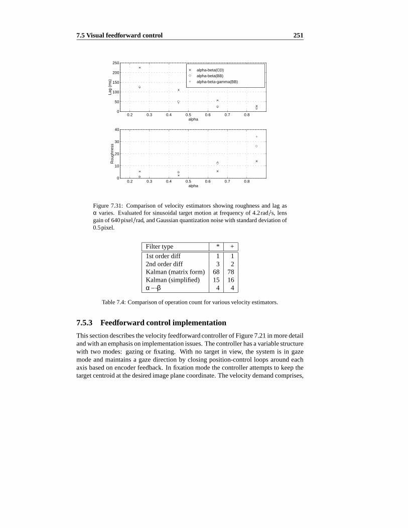
7.5Visual feedforward control 251
0.2 0.3 0.4 0.5 0.6 0.7 0.80
10
20
30
40
alpha
Rou
ghne
ss0.2 0.3 0.4 0.5 0.6 0.7 0.8
0
50
100
150
200
250
alpha
Lag
(ms)
alpha-beta(CD)
alpha-beta(BB)
alpha-beta-gamma(BB)
Figure7.31: Comparisonof velocity estimatorsshowing roughnessand lag asα varies. Evaluatedfor sinusoidaltarget motion at frequency of 4.2rad s, lensgainof 640pixel rad, andGaussianquantizationnoisewith standarddeviationof0.5pixel.
Filter type * +
1storderdiff 1 12ndorderdiff 3 2Kalman(matrix form) 68 78Kalman(simplified) 15 16α β 4 4
Table7.4: Comparisonof operationcountfor variousvelocityestimators.
7.5.3 Feedforward control implementation
Thissectiondescribesthevelocityfeedforwardcontrollerof Figure7.21in moredetailandwith anemphasisonimplementationissues.Thecontrollerhasavariablestructurewith two modes:gazingor fixating. With no target in view, the systemis in gazemodeandmaintainsa gazedirectionby closingposition-controlloopsaroundeachaxisbasedon encoderfeedback.In fixation modethecontrollerattemptsto keepthetargetcentroidat thedesiredimageplanecoordinate.Thevelocitydemandcomprises,

252 Control designand performance
Activevideo
Pixelsexposed
Joint anglesread
Current commandsent
Pixel transportand processing
Control lawcalculation
θ
Video field time (20ms)
Time
Video blankingtime (1.6ms)
Figure7.32: Detailsof systemtiming for velocity feedforwardcontroller. Notethe small time delaybetweenbetweenthe centerof the pixel exposureintervalandthejoint anglesbeingread;in practicethis is around1.3ms.
for eachDOF, predictedtarget velocity feedforwardandimageplanecentroiderrorfeedback
xd ˆxtiKp
i XiKi
i Xdt if i X i∆0 otherwise
(7.62)
Whenthetarget is within a designatedregion aboutthedesiredimageplanecentroidintegralactionis enabled.Theintegral is resetcontinuouslywhenthetargetis outsidethis region. Both α β andKalmanfilters have beenusedfor velocity estimation,ˆxt , in this work. Thetransitionfrom gazingto fixation involvesinitiating thetrackingfilters.No visionbasedmotionis alloweduntil thetargethasbeenin view for at leasttwo consecutive fields in orderto computea crudetarget velocity estimatefor filterinitiation. Intuitively it is unproductive to startmoving uponfirst sightingthe targetsince its velocity is unknown, and the robot may start moving in quite the wrongdirection.
The pan and tilt axis axis velocitiesare controlledby two digital axis-velocityloops as describedin Section7.5.1. Thereis explicit correctionfor the wrist axiscross-coupling(2.38).Themotor-referencedjoint velocitiesare
θ5 G5ωt il t (7.63)
θ6 G6ωpan G56G6ωt il t (7.64)

7.5Visual feedforward control 253
Demux
Demux1
PID
PID Controller
−1
Switch
Linkangle
−+
Relativeview
1
Gazegain
+−
Pixelerror
0
Constant
Switch
swvloopi
s/wvloop
Scope1
kalfilt
Target est
Demux
DemuxEst.velocity
Target path
z1
Unit Delay
Quantnoise
.5
StdDev
+
+
Addnoise
z
1
Visionsystem
Mux
Mux
634
Lens
MATLABFunction
Outputdecouple
Targetpos
Scope
+−
Sum2
Clock
Mux
Mux5
yTo Workspace
Figure7.33:SIMULINK modelFFVSERVO: feedforwardfixationcontroller.
Figure7.32shows detailsof thetiming relationshipsinvolved. Theactualinstantof camerasamplingis not signalledby the camera,but hasbeendeterminedexperi-mentallyin Figure3.14with respectto thevideowaveform. Theshortexposuretimeis requiredin orderthat the cameraapproximatean idealsamplerof thevisual statewhich is assumedfor thecontroldesign.Motion blur is not significantsincefixationkeepsthetargetfixedwith respectto thecamera.Therobot'sjoint anglesaresampledby ataskduringtheverticalblankingintervalandcombinedwith theimageplanecen-troid using(7.43)to estimatethetargetposition.Thereis somefinite time differencebetweensamplingthejoint anglesandpixelexposure.Analysisof systemtimestampsindicatesthat this averages1.3mswith a standarddeviation of 0.11ms. It would bepossibleto usefirst-orderpredictorsto computejoint anglesat the video samplinginstantbut thishasnotbeenattempted.
A single-axisSIMULINK model, shown in Figure 7.33, was createdto verifythe overall operationandto assistin initial controlparameterselection.Figure7.34showsthesimulatedperformancewhentrackingthestandardtargetmotionwith peakvelocity of 1radl s. It canbeseenthatthetargetvelocity estimatoris providing mostof thevelocitydemand,but thatthis feedforwardsignalis laggingtheaxisvelocitybyapproximately70ms. This is dueto lag in thevelocity estimatorasdiscussedabove,andalsotheunit delayonpositiondatabeingpassedto thevelocity estimator.

254 Control designand performance
0 0.5 1 1.5 2 2.5 3 3.5 4 4.5 5-2
-1
0
1
2
3
Time (s)
Axi
s ve
l (ra
dl/s
)
0 0.5 1 1.5 2 2.5 3 3.5 4 4.5 5-60
-40
-20
0
20
40
Time (s)
Err
or (
pix)
Figure7.34:Simulationof feedforwardfixationcontrollerfor standardtargetmo-tion. Top plot shows total axis velocity demand(solid) andestimatedtarget ve-locity (dashed).Bottom plot shows the target centroiderror. RMS pixel error,excludingtheinitial transient,is 11pixels. (iKp 0 03, iKi 0 0042.)
Tilt
Pan
Turntable
Figure7.35:Turntablefixationexperiment

7.5Visual feedforward control 255
7.5.4 Experimental results
A numberof experimentshave beenconductedto investigatetheperformanceof thefixation controller. To achieve a particularlychallengingmotionfor thetrackingcon-troller a turntablehasbeenbuilt whoserotationalvelocitycanbeconstant,or arevers-ing trapezoidalprofile. At maximumrotationalspeedof 40rpm theformerprovidestargetswith thestandardmotiondescribedin (7.10). Thereversingprofile resultsintargetmotionwith acomplex Cartesianaccelerationprofile.
In thefirst experimentthecamerais fixatedon a target rotatingon a turntableasshown in Figure7.35. The turntableis rotatingat the standardtrajectory's angularvelocity 4.2rad s. Figure7.36shows the imageplanecoordinateerror in pixels. Itcanbeseenthat thethe target is keptwithin 15pixelsof thereference.Theearlier,feedback-onlystrategy resultsin large following errorsanda lag of over 40 . Fig-ure7.37shows themeasuredandfeedforwardjoint velocity for thepanandtilt axes.Thejoint velocity of up to 2radl s is closeto the limit of theUnimatevelocity loop,2.3radl s. Thefeedforwardvelocitysignalhasthesamemagnitudeasthevelocityde-mandbut is slightly lagging,aswasthecasefor thesimulation.Theothercomponentof thevelocity demandis providedby thePI feedbacklaw which is necessaryto
achieve zeropositionerror tracking,sincematchingtarget androbot velocitystill allowsfor anarbitraryconstantpositionerror;
overcomelagsin thefeedforwardvelocitydemandandthevelocity loop itself;
rejectthedisturbanceintroducedby a targetwhosecentroidlies off theopticalaxis which will appearto rotatearoundtheprincipalpoint asthecamerarollsdueto motionof joints5 and6 by (6.7);
accommodatetheposedependentgainrelatingθ5 to tilt ratein (6.6).
Thecontrolleris quiterobustto errorsin thelensgainestimateusedin (7.43).Duringfixationthecentroiderrori X is small,sominimizingthesignificanceof errorsin Klens.
A disturbancemaybegeneratedby usingtheteachpendantto move thefirst threerobot joints. Thefixation controlleris ableto counterthis disturbancebut therejec-tion dynamicshave not beeninvestigated.The disturbancecouldalsobe counteredby feedingforwardthecamerapan/tilt ratesdueto themotionof thosejoints. Suchastructurewould thenbesimilar to thehumaneye in thattheeye musclesacceptfeed-backfrom theretina,aswell asfeedforwardinformationfrom thevestibular system,givingheadlateralandrotationalacceleration,andheadpositioninformationfrom theneckmuscles.
Figure7.38showsthesetupfor anexperimentwherethecamerafixatesonaping-pongball thrown acrossthe system's field of view. Experimentalresultsshown inFigure7.39 areobtainedwith the samecontrolleras the previous experiment. Therecordedevent is very brief, lastingapproximately700ms. Trackingceaseswhenthe

256 Control designand performance
0 2 4 6 8 10-20
-10
0
10
20
Time (s)
Y e
rror
(pi
xels
)0 2 4 6 8 10
-20
-10
0
10
20
30
Time (s)
X e
rror
(pi
xels
)
Figure 7.36: Measuredtracking performance,centroid error, for target onturntablerevolving at4.2rad s. Thisdatawasloggedby RTVL.
0 2 4 6 8 10-2
-1
0
1
2
3
Time (s)
X-a
xis
velo
city
(ra
dl/s
)
0 2 4 6 8 10-4
-2
0
2
4
Time (s)
Y-a
xis
velo
city
(ra
dl/s
)
Figure 7.37: Measuredtracking velocity for target on turntablerevolving at4.2rad s, showing axis velocity (solid) and estimatedtarget velocity (dashed).Note that the Y-axis (tilt) velocity is somewhat triangular— this is due to the1 S6 termin thetilt kinematicsgivenby (6.6).Thisdatawasloggedby RTVL.

7.6Biological parallels 257
Tilt
PanBall
Figure7.38:Pingpongball fixationexperiment
ball disappearsfrom view asit movesinto a poorly lit region of thelaboratory. Fromthecentroiderrorplot it canbeseenthattherobotachievesanapproximatelyconstantcentroiderrorof lessthan30pixelsin thevertical,Y, directionin which the ball hasconstantacceleration.In thehorizontal,X, directiontherobotis seento have overshotthetarget. Themeasuredjoint velocitiesshow a peakof over 4radl son thetilt axis,which hasa limit dueto voltagesaturationof 5radl s. Theapparentsizeof theball(area)canbeseento varywith its distancefrom thecamera.Thetrackingfilter in thiscaseis aKalmanfilter wherethetimevaryinggainis anadvantagegiventhetransientnatureof theevent. Therobotdoesnot commencemoving until theball hasbeeninthefield of view for a few field timesin orderfor theKalmanfilter stateestimatestoconverge.
7.6 Biological parallels
Therearesomeinterestingparallelsbetweenthecontrolmodelsdevelopedhereusingcontrolsystemanalysisandsynthesis,andthoseproposedto explain theoperationofthehumanvisualfixationreflex. Robinson[214] investigatesthecontrolof twohumanvisualbehaviours,saccadicmotionandsmoothpursuit,andhow instabilityis avoidedgiventhepresenceof significantdelayin neuralsensingandactuation'circuits'. Thesmoothpursuitreflex operatesfor targetmotionup to 100deg s andexperimentsre-veal that the responseis characterizedby a delayof 130ms anda timeconstantof40ms.Thedelayis partitionedas50msfor theneuralsystemand80msfor peripheral(muscle)delay. Sachadiceye motionsareusedto directthefoveato apointof interestandcanbeconsideredas'open-loop' plannedmoves. Theneuraldelayfor saccadicmotionis 120mscomparedto 50msfor fixation motion,andindicatesthatfixation isa lower level andmorereflexive action.
For a constantvelocity target the eye achievesa steady-statevelocity of 90%ofthe target velocity, that is, the oculomotorsystemis of Type 0. Thereis alsophysi-

258 Control designand performance
0 0.1 0.2 0.3 0.4 0.5 0.6 0.7 0.8
0
100
200
Time (s)
Cen
troi
d er
r (p
ix)
Xc
Yc
0 0.1 0.2 0.3 0.4 0.5 0.6 0.7 0.8-4
-2
0
2
Time (s)
Axi
s ve
l (ra
dl/s
)
pan
tilt
0 0.1 0.2 0.3 0.4 0.5 0.6 0.7 0.8
50
100
Time (s)
Are
a (p
ix^2
)
Figure7.39: Measuredtrackingperformancefor flying ping-pongball. Shownarecentroiderror, link velocityandobservedareaof target. Thisdatawasloggedby RTVL.
ologicalevidencethattheoculomotorcontrolsystemcanbeconsidereda continuoustimesystem.Like therobotvisualservo systemdiscussedearlier, theeye controllerisdrivenby retinalpositionor velocitywhichmeasuresdirectly theerrorbetweentargetandeye direction. Sincethesystemis drivenby anerrorsignalit is a negative feed-backsystemwhich admitsthepossibilityof stability problems.However despitethesignificantdelaysin thesensorandactuatorthis feedbacksystemis stable.To explainhow themechanismavoidedinstabilityheproposestheexistenceof aninnerpositive-feedbackloop thatcancelstheeffect of thepotentiallyproblematicnegative-feedbackloop. This structureis shown in block diagramform in Figure7.40. Ideally the twofeedbackpathscancelso the resultingdynamicsare dictatedby the forward path.Suchanexplanationis somewhatbizarrefrom a controlsystemspointof view where'positive feedback'is generallyconsideredassomethingto beavoided.However theproposedmodelcanbe interpreted,seeFigure7.41,asbeingstructurallysimilar tothevelocity feedforwardcontroldescribedin theprevioussection.The effect of the

7.6Biological parallels 259
+
X.i
-0.9
0.04s 1+
neuralV s( )
+
x.r
+
P s( )
actuator
80
50 50 30
P2
P1
R s( )
x.d
x.t
x.t
Figure7.40:Proposedmodelof oculomotorcontrolsystemafterRobinson[214]with somenotationaldifferencesto conformwith this work. Squareboxescon-tainingnumbersrepresentpuretimedelayin unitsof milliseconds.P1 andP2 areadaptivegains.Actuatordynamicsaretakento beP s 1.
xrx.d
Xi
1
z
D z( )
V z( ) R z( )+
xt z( )
-
compensator
robotvision
targetposition
E z( )
velocity
++
P z( )
target
xtx.t
positionestimator
estimator
+
+
Figure7.41:Rearrangementof Figure7.21to show similarity to Robinson'spro-posedoculomotorcontrol system.P z is definedby (7.43)andis essentiallyasummation.Thepathshown dottedrepresentsthelesssignificantfeedbackpath,which if eliminatedresultsin astructurethatis identicalto Robinson's.
positive feedbackis to createan estimateof the target velocity, basedon measuredretinal velocity anddelayedeye velocity command. The feedforwardcontrollerofFigure7.21is very similar except that target positionis estimatedfrom 'retinal' andmotorpositioninformationandthendifferentiatedto form theprincipalcomponentofthemotorvelocitysignal.
Eliminatingnegative feedback,asshown in themodelof Figure7.40,alsoelimi-natesits benefits,particularlyrobustnessto parametervariations.In a biologicalsys-temthesevariationsmaybecausedby injury, diseaseor ageing.Robinsonproposesthatparameteradaptionoccurs,modelledby the gain termsP1 andP2, andprovidesexperimentalevidenceto supportthis. Such'plasticity' in neuralcircuits is commonto much motor learningand involves changeover timescalesmeasuredin daysor

260 Control designand performance
evenweeks.Parametervariationagainadmitsinstability, if for instancethepositive-feedbackgain is greaterthanthenegative-feedbackgain. Robinson'spaperdoesnotdiscussthedynamicsof theactuatorapartfrom time delay, but it maybethat for eyeactuationinertiaforcesareinsignificant.
7.7 Summary
Theuseof machinevision for high-performancemotioncontrol is a significantchal-lengedueto theinnatecharacteristicsof thevisionsensorwhichincluderelatively lowsamplerate,latency andsignificantquantization.Many of thereportsin theliteratureuselow loop gainsto achieve stable,but low-speed,closed-loopvisualcontrol.
The simpleandcommonlyusedproportionalfeedbackcontroller, while demon-stratingan adequatestepresponse,haspoor tracking performance. Compensatordesign,to improve this performance,hasfollowed classicallinear principlesof in-creasingsystemTypeandpositioningtheclosed-looppolesby meansof PID or pole-placementcontrol. It hasbeenfound that the closed-looppolescannotbe madear-bitrarily fastandareconstrainedby a practicalrequirementfor compensatorstability.This instabilityis believedto bedueto modellingerrors,or plantnon-linearitieswhichleadto modelerrorsatsaturation.
It is difficult to quantitatively comparetheperformanceof this systemwith otherreportsin the literature,due largely to the lack of any commonperformancemet-rics. A trackingperformancemeasurewasdefinedin termsof imageplaneerror fora standardsinusoidaltarget motion. A numberof reportson robot heads[231,270]cite impressive peakvelocity andaccelerationcapabilities,but theseareachievedforsaccadicnot closed-loopvisuallyguidedmotion.Many reportsprovidestepresponsedataandthisgivessomemeasureof closed-loopbandwidthbut it hasbeenshown thatphasecharacteristicsarecritical in trackingapplications.
The experimentalconfigurationusedin this work, like the majority of reportedexperimentalsystems,implementsa visual feedbackloop aroundthe robot's exist-ing position-controlloops. However it hasbeenshown that the redundantlevels ofcontroladdto systemcomplexity andcanreduceclosed-loopperformanceby increas-ing open-looplatency. Investigationof alternativecontrolstructuresbasedonvariousunderlyingaxis-controlmethodsconcludedthat axis feedback,at the leastvelocityfeedback,is requiredto give acceptableperformancegiven the low visual samplingrateandthenon-idealityof a realrobotaxis.
Thedesignconstraintsinherentin feedback-onlycontrolleadto theconsiderationof feedforwardcontrol,which givesadditionaldesigndegreesof freedomby manip-ulatingsystemzeros.A 2-DOF variable-structurevelocity-feedforwardcontrollerisintroducedwhich is capableof high-performancetrackingwithout thestability prob-lems associatedwith feedback-onlycontrol. The feedforwardapproacheffectivelytransformstheproblemfrom controlsynthesisto motionestimation.

7.7Summary 261
Thenext chapterextendstheprinciplesdevelopedin thischapter, andappliesthemto visualservoing for directend-pointcontrolandto 3-DOFtranslationaltracking.

262 Control designand performance

Chapter 8
Further experimentsin visualservoing
Thischapterextends,andbringstogether, theprinciplesdevelopedin earlierchapters.Two examples,both involving dynamicvisualservoing, will bepresented.Firstly 1-DOFvisualcontrolof amajorrobotaxiswill beinvestigatedwith particularemphasisontheendpointratherthanaxismotion.Secondly, planartranslationalcameracontrolwill be investigatedwhich requirescoordinatedmotion of the robot's 3 baseaxes.Thesimple2-DOFcontrolof thepreviouschaptereffectively decoupledthedynamicsof eachaxis, with oneactuatorper cameraDOF. In this casethereis considerablekinematicanddynamiccouplingbetweenthe axes involved. This chaptermust,bynecessity, addressa numberof issuesin robot or motion control suchascontrollerstructureartifacts,friction andstructuraldynamics.Many of thesetopicshave beenintroducedpreviouslyandwill notbedealtwith in greatdetailhere;rathera'solution'orientedapproachwill betaken.
8.1 Visual control of a major axis
Previous sectionshave describedthe visual control of the robot's wrist axes,whicharealmostideal,in thatthey have low inertiaandfriction andarefreefrom structuralresonancesin thefrequency rangeof interest.Thissectioninvestigatestheapplicationof visualservoing to thecontrolof a majorrobotaxis,in this casethewaistaxis,andit will beshown thatthecontrolproblemis non-trivial dueto 'real-world'effectssuchassignificantnon-linearfriction andstructuralresonances.
In thisexperimentthecamerais mountedontherobot'send-effector, whichmovesin ahorizontalplaneoveraworktableonwhichthetargetobjectsitsatalocationthatis
263

264 Further experimentsin visual servoing
30deg
Start of swing pose
End of swing pose with cameraover target.
969mm
θ1
XcYc
Figure8.1: Planview of theexperimentalsetupfor majoraxiscontrol.
only approximatelyknown. Therobot'swaistjoint swingsthroughapproximately30andis visually servoedto stopwith thecameradirectly over thetarget. Only 1-DOFis controlled,sothecamera's truemotionis anarcandthepositioningis suchthattheX-coordinateof the target's imageis broughtto thedesiredimageplanelocation. Aschematicplanview is shown in Figure8.1.
Thisexperimenthassomesimilarity with thewayin whichrobotsareusedto per-form partplacementin planarassemblyapplicationssuchasPCBmanufacture.Thatrole is typically performedby high-speedSCARA robotswhich mustmove quicklyfrom part feederto thepart location,settle,andthenreleasethe part. Electronicas-semblyrobotssuchastheAdeptOnearecapableof positioningaccuracy of 75µm andend-effectorspeedsof 9m s.
8.1.1 The experimentalsetup
Thecameralooksdownwardtowardthetable.As thecameraswingstowardthetarget,thetargetappearsto movein thenegativeX directionwith respectto thecamera's co-ordinateframe.TheX componentof thetarget'scentroidis takenasa measureof thecamera's positionrelative to thetarget.Therobotarmis well extendedsothata largeinertiais 'seen'by thejoint 1 axis.Thearmposeis θ1 18 123 0 14 90 , andusingtherigid-bodydynamicmodelfromSection2.2.4yieldsaninertiafor joint 1 dueto link andarmatureinertiasof 3 92kg m2. Thecamerainertia,computedfrom knownmassandrotationradius,is 0.970kg m2. Thetotal inertiaat thelink is 4.89kg m2, orin normalizedform, 7 5Jm1. In this posethecamerarotationalradius1 is 969mmand
1Thedistancebetweenthejoint 1 rotationalaxisandtheopticalaxisof thecamera.
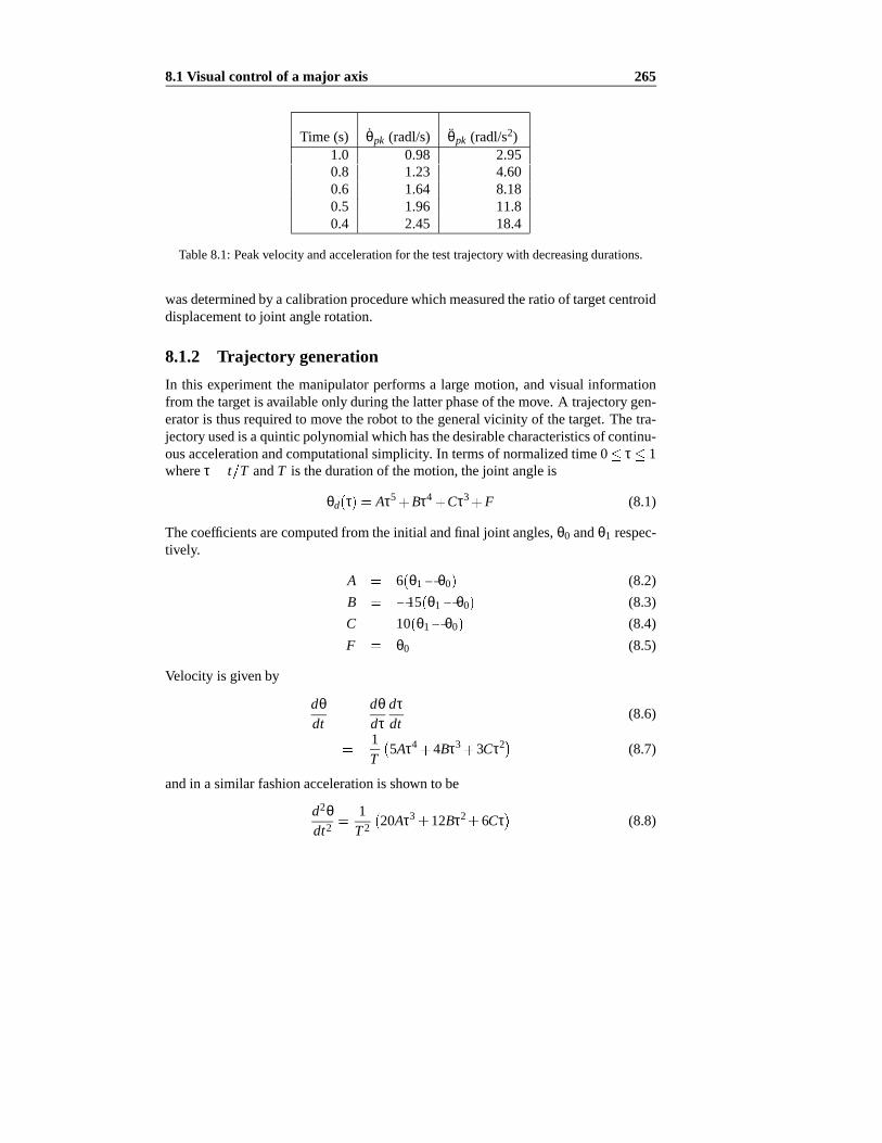
8.1Visual control of a major axis 265
Time (s) θpk (radl/s) θpk (radl/s2)1.0 0.98 2.950.8 1.23 4.600.6 1.64 8.180.5 1.96 11.80.4 2.45 18.4
Table8.1: Peakvelocityandaccelerationfor thetesttrajectorywith decreasingdurations.
wasdeterminedby acalibrationprocedurewhichmeasuredtheratioof targetcentroiddisplacementto joint anglerotation.
8.1.2 Trajectory generation
In this experimentthe manipulatorperformsa large motion, andvisual informationfrom thetargetis availableonly duringthelatterphaseof themove. A trajectorygen-eratoris thusrequiredto move therobotto thegeneralvicinity of thetarget. Thetra-jectoryusedis aquinticpolynomialwhichhasthedesirablecharacteristicsof continu-ousaccelerationandcomputationalsimplicity. In termsof normalizedtime0 τ 1whereτ t T andT is thedurationof themotion,thejoint angleis
θd τ Aτ5 Bτ4 Cτ3 F (8.1)
Thecoefficientsarecomputedfrom theinitial andfinal joint angles,θ0 andθ1 respec-tively.
A 6 θ1 θ0 (8.2)
B 15 θ1 θ0 (8.3)
C 10 θ1 θ0 (8.4)
F θ0 (8.5)
Velocity is givenby
dθdt
dθdτ
dτdt
(8.6)
1T
5Aτ4 4Bτ3 3Cτ2 (8.7)
andin a similar fashionaccelerationis shown to be
d2θdt2
1T2 20Aτ3 12Bτ2 6Cτ (8.8)

266 Further experimentsin visual servoing
0 0.05 0.1 0.15 0.2 0.25 0.3 0.35 0.4 0.45 0.50
0.5
1
Time (s)
q(t)
(ra
dl)
0 0.05 0.1 0.15 0.2 0.25 0.3 0.35 0.4 0.45 0.5-2
-1
0
Time (s)
qd(t
) (r
adl/s
)
0 0.05 0.1 0.15 0.2 0.25 0.3 0.35 0.4 0.45 0.5-20
0
20
Time (s)
qdd(
t) (
radl
/s2)
Figure8.2: Position,velocityandaccelerationprofileof thequinticpolynomial.
Theminimumachievablemove durationwill ultimatelybelimited by friction andamplifiervoltageandcurrentsaturation.Thepeakvelocitiesandaccelerationsfor thistrajectoryhave beencomputedfor a numberof time intervals,andtheseresultsaresummarizedin Table8.1. Basedon the manipulatorperformancelimits from Table2.21it is clearthatthe0.5strajectoryis atapproximatelythevelocity limit for joint 1,andwill beselectedasthereferencetrajectoryfor this section.Figure8.2 shows thecomputedpositionandvelocityasa functionof time for a0.5sswingover 30 .
Theaveragejoint velocityis 1radl swhichin thisposeresultsin anaveragetrans-lationalvelocity of around1000mm s, thequotedlimit of thePuma560[255]. Thepeakcameratranslationalvelocity is almost2000mm s, whichwith anexposuretimeof 2mswouldresultin amaximummotionblur of 4mmcausinga laggingimagecen-troid estimateandsomedistortionof the target image.Theseeffectsdecreaseastherobotslowsdown onapproachto thetarget.
8.1.3 Puma 'native' position control
Jointpositioncontrol is performedby theUnimatepositioncontrolsystemdescribedpreviously in Section2.3.6. Thehostissuessetpointscomputedusing(8.1) at 14msintervalsandthesearepassedto thedigital axisservo. This interpolatesbetweenthe

8.1Visual control of a major axis 267
0 0.1 0.2 0.3 0.4 0.5 0.6 0.7 0.80
0.2
0.4
Time (s)
j1
0 0.1 0.2 0.3 0.4 0.5 0.6 0.7 0.8
-100
1020
Time (s)
j1dd
0 0.1 0.2 0.3 0.4 0.5 0.6 0.7 0.8
-1.5-1
-0.50
j1d
Figure8.3: Measuredaxisresponsefor Unimatepositioncontrol,showing posi-tion, velocity andacceleration:measured(solid) anddemand(dotted).Datawasrecordedby theRTVL systemat14msintervals,andanoff-line procedureusing5-pointnumericaldifferentiationwasusedto obtainthe'measured'velocity andaccelerationdata. Note the stepdecelerationat 0.45s or 70ms beforethe firstzerocrossingof themeasuredvelocity. All quantitiesareloadreferenced,anglesin radians.
positionsetpointsemittedby thetrajectorygeneratorandclosesapositionlooparoundtherobot'sanalogvelocity loopata samplerateof approximately1kHz.
Theperformanceof theUnimateservo systemis shown in Figure8.3whichcom-paresthedemandedandmeasuredaxisposition,velocity andacceleration.It canbeseenthatthemeasuredjoint anglelagsconsiderablybehindthedesiredjoint angleandthat theaxisvelocity has'bottomedout' between0.25and0.45s. Thelimiting valueof -1.6radl s is dueto velocity loopsaturation.Table2.20predictsa velocity limit of1.42radl sfor joint 1 which is of a similarorderto thatobservedin this experiment2.Thepositionloop hasvery high gainandit canbeshown from Section2.3.6that thevelocity loopdemandwill besaturatedfor positionerrorgreaterthan0.018radlor 1 .By t 0 45spositionerror is sufficiently small that thevelocity demandrisesabovethesaturationlevel andtheaxisbegins to decelerateandtheaccelerationplot shows
2Gainvariationin theanalogelectronics,mentionedin Section2.3.6,or friction variationmayaccountfor thisdiscrepancy.

268 Further experimentsin visual servoing
0 0.05 0.1 0.15 0.2 0.25 0.3 0.35 0.4-0.03
-0.02
-0.01
0
0.01
Time (s)
q1 (
radl
)
0 0.05 0.1 0.15 0.2 0.25 0.3 0.35 0.4-40
-20
0
20
40
Time (s)
Xdd
_cam
(m
/s^2
)
Figure8.4: Measuredjoint angleandcameraaccelerationunderUnimatepositioncontrol. Datawasrecordedwith a 2-channeldata-acquisitionunit andthe timescalesof this figurearenot alignedwith thoseof Figure8.3. However theonsetof oscillationis around70msbeforethejoint anglepeak.
a stepoccurringat this time. Considerabledecelerationcanbeachievedsinceback-EMF actsto increasemotor currentwhich will thenbe limited by the currentloop,while Coulombandviscousfriction alsosupplydeceleratingtorque.
Figure8.4showstheresponseof themotorjoint angleandthecameraaccelerationfor the0.5strajectoryrecordedusinga2-channeldata-acquisitionunit. Thejoint anglehasovershotby 8 3 10 3radlresultingin acameraovershootof 8mm. Fromtheplotof cameraaccelerationthereis clearlyconsiderableoscillationof thecamera,peakingat 4g. Thehigh decelerationcausedby theaxis controller, shown in Figure8.3,hasexcitedaresonancein themanipulatorstructureataround20Hz. Thelargeoscillationbetween0.10 and0.15s hasan amplitudeof approximately15m s2 correspondingto a displacementamplitudeof 1mm. The lower level vibrationpresentafter0.25scorrespondsto a displacementamplitudeof around0 3mmwhich is significantlylessthan1pixel. Figure8.5comparesthedisplacementof thecameradeterminedby twodifferentmeans.Over thesmallangularrangeinvolvedin motionnearthetarget,theend-effectorpositioncanberelateddirectly to link angle,θ1, by
xm rθ1 (8.9)

8.1Visual control of a major axis 269
wherer is the radiusof camerarotation. The displacementcanalsobe determinedfrom thecamera
xc KlensiX (8.10)
wherethe lens gain, in this translationalcontrol case,will be a function of targetdistanceasdiscussedin Section6.3.2.Lensgainwasdeterminedfromtheimageplanedistancebetweenthecentroidsof calibrationmarkerswith known spacing,resultingin an estimateKlens 0 766mm pixel. Figure 8.5 is derived from dataloggedbythe controller itself. Timestampson target centroiddataindicatethe time at whichthe region datawas fetchedfrom the APA-512, not when the camerapixels wereexposed.However thevideo-lockedtimestampingsystemallowstheexposuretimetobeestimated,andthis is usedwhenplottingcentroiddatain Figure8.5.Thereis goodcorrespondencebetweenthe two measurementsas the robot approachesthe target3.Howeverat thepeakof theovershootthevisionsystemindicatesthatthedisplacementis 1.9mmgreaterthanthatindicatedby theaxis.Datarecordedduringtheexperimentalsoindicatesthatjoints4 and6 rotateby 1 5 10 3 and6 10 4radlduringthispartof thetrajectory, dueto inertial forcesactingonthecamera.In thispose,suchrotationwould tendto reducethevisually perceivedovershoot.FromFigure8.5 thedampednaturalfrequency of the overshootmotion is approximately7Hz andthis would belargely a function of the Unimatepositionloop. As discussedin Section2.3.6 theswitchableintegral action featureof the position loop4 resultsin a poorly-dampedlow-frequency pole pair. With integral actiondisabledthe overshootis only 60%ofthat shown in Figure8.4 andthereis no subsequentundershoot.However the axisstops37 10 3radm(6encoders) or 0.5mmshortof thetargetdueto friction effects.
8.1.4 Understandingjoint 1 dynamics
The purposeof this sectionis to develop a simple model of the joint 1 dynamicswhich includesstructuralresonancein the transmissionand the electro-mechanicaldynamicsof the motor andcurrentloop. Figure8.6 shows the measuredfrequencyresponsefunctionbetweenmotorshaftangleandaccelerationof the camera,for therobot in the standardposeusedfor this experiment. Thereare3 structuralmodesin the frequency rangemeasured:thefirst occursat 19Hz which is below the 25HzvisualNyquist frequency; theothersareabove theNyquist frequency andmayresultin aliasing.
3Thereis evidencethatthejoint anglemeasurementlagsapproximately2msbehindthevisionmeasure-ment. This maybe dueto incorrectcompensationof timestampedcentroiddata,or overheadandtimingskew in readingencoderdatafrom theUnimatedigital servo board.In additiontheencodervaluereturnedby the servo is the valueat the last clock period. Furtherrefinementof measurementtimeswill not bepursued.
4Integralactionis configuredto switchin whentheaxisis within 50encodercountsof thetargetwhichis 0.005radlfor thisaxis.
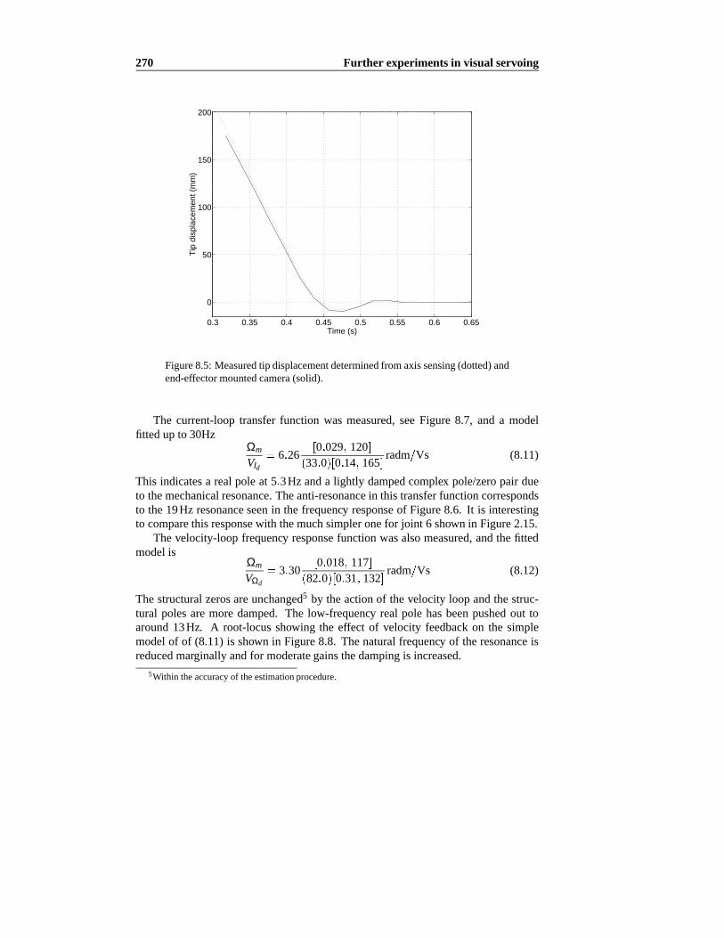
270 Further experimentsin visual servoing
0.3 0.35 0.4 0.45 0.5 0.55 0.6 0.65
0
50
100
150
200
Time (s)
Tip
dis
plac
emen
t (m
m)
Figure8.5: Measuredtip displacementdeterminedfrom axissensing(dotted)andend-effectormountedcamera(solid).
The current-looptransferfunction was measured,seeFigure 8.7, and a modelfittedup to 30Hz
Ωm
VId6 26
0 029 12033 0 0 14 165
radm Vs (8.11)
This indicatesa realpoleat 5 3Hz anda lightly dampedcomplex pole/zeropair dueto themechanicalresonance.Theanti-resonancein this transferfunctioncorrespondsto the19Hz resonanceseenin the frequency responseof Figure8.6. It is interestingto comparethis responsewith themuchsimpleronefor joint 6 shown in Figure2.15.
Thevelocity-loopfrequency responsefunctionwasalsomeasured,andthefittedmodelis
Ωm
VΩd
3 300 018 117
82 0 0 31 132radm Vs (8.12)
Thestructuralzerosareunchanged5 by theactionof thevelocity loop andthestruc-tural polesaremoredamped. The low-frequency real pole hasbeenpushedout toaround13Hz. A root-locusshowing the effect of velocity feedbackon the simplemodelof of (8.11) is shown in Figure8.8. Thenaturalfrequency of theresonanceisreducedmarginally andfor moderategainsthedampingis increased.
5Within theaccuracyof theestimationprocedure.

8.1Visual control of a major axis 271
101
102
-100
0
100
Freq (Hz)
Pha
se (
deg)
101
102
-20
0
20
Freq (Hz)
Mag
(dB
)
Figure8.6: Measuredfrequency responsefunction 1 jω 2Xcam Θm which in-cludesarmstructureandtransmissiondynamics.Thefirst resonanceis at 19Hz.Goodcoherencewasobtainedabove4Hz.
The main aspectsof the joint 1 dynamicsareaccountedfor by the simpletwo-inertiamodelshown in Figure8.9. In thismodelJm representsthemotorinertiaandJl
themotor-referencedinertiaof thearmandcamera.Elasticityandenergy dissipationin the transmission,physicallydueto torsionalcompliancein the long vertical driveshaftbetweenthebull gearandlink 1, aremodelledby thespringK anddamperB.Motor friction is representedby Bm, andmotorelectricaltorqueis τm.
Laplacetransformedequationsof motionfor this systemmaybewritten
s2JmΘm τm BmsΘm Bs K Θm Θl (8.13)
s2Jl Θl Bs K Θm Θl (8.14)
Thesereduceto thetransferfunctions
Ωm
τm
sΘm
τm
Jl s2 Bs K
∆(8.15)
Ωl
τm
sΘl
τm
Bs K∆
(8.16)

272 Further experimentsin visual servoing
100
101
-30
-20
-10
0
10
20
Frequency (Hz)
Mag
(dB
)
Figure8.7: Measuredfrequency responsefunction magnitudefor joint 1 motorandcurrentloopΩm s VId s .
where
∆ JmJl s3 Jm Jl B BmJl s2 Jm Jl K BBm s KBm (8.17)
Thetransferfunctionfrom motorpositionto loadposition,measuredin Figure8.6,isgivenby thissimplemodelas
Θl
Θm
Bs KJl s2 Bs K
(8.18)
σ0
ζ0 ω0(8.19)
in theshorthandnotationemployedpreviously. Thenumeratorof thetransferfunction(8.15)is thesameasthedenominatorof (8.18)andthiswasobservedin themeasuredtransferfunctionsshown in Figures8.6and8.7. In (8.19),
σ0KB
(8.20)
ω0KJl
(8.21)

8.1Visual control of a major axis 273
-300 -250 -200 -150 -100 -50 0 50 100-200
-150
-100
-50
0
50
100
150
200
Real Axis
Imag
Axi
s
Figure8.8: Root-locusfor motor and currentloop with single-modestructuralmodel. The markedclosed-looppolescorrespondto a loop gain of 11.5whichplacestherealcurrentlooppoleat-82rad sasfor thevelocity-loopmodel(8.12).
K
B
Bm
θm θt
τm
Jm Jl
Figure8.9: Schematicof simpletwo-inertiamodel.
ζ0B
2 KJl(8.22)
Inspectionof Figure8.6 indicatesthatω0 2π 19Hz (ω0 120rad s) andthatσ0
is at someconsiderablyhigher frequency. From (8.21) it is clear that the resonantfrequency decreasesasthe 'outboard' inertia,Jl , increases.Theselectedrobotposehasalmostmaximumpossibleinertiaaboutthejoint 1 axisthusbringingtheresonance
274 Further experimentsin visual servoing
aslow aspossible.Consideringnow themotorcurrent-to-velocitytransferfunctionmeasuredin Fig-
ure8.7,themodelversionis, from (8.15)and(8.17),
Ωm
τm
1Bm
ζ0 ω0
σ ζ ωn(8.23)
Theexperimentalmodel(8.11)indicatesthat
ω0 120 (8.24)
ζ0 0 029 (8.25)
σ 33 (8.26)
ω 165 (8.27)
ζ 0 14 (8.28)
Using the previously obtainedestimateof Jm Jl 7 5Jm, andthe parametervalueJm 200 10 6kg m2, it canbededucedthat
Jl 1 3 10 3kg m2 (8.29)
K Jl ω20 18 7N m s rad (8.30)
B 2ζ0 KJl 9 05 10 3N m s rad (8.31)
Bm 0 032N m s rad (8.32)
Henceσ0 K B 2069rad s (329Hz), too high to berevealedin themeasurementof Figure8.6.
If therewasno compliancein thetransmissionfrom motor to load, (8.15)wouldreduceto
Ωm
τm
1Jm Jl s Bm
(8.33)
1 Bm
σ1(8.34)
whereσ1 Bm Jm Jl . Therealpoleof thecompliantsystemats σ is differentfrom σ1. Numericalinvestigationshowsthatfor for highstiffnessandlow dampingσ will bevery closeto but slightly morenegative thanσ1.
8.1.5 Single-axiscomputedtorquecontrol
As apreludeto trialing visualservo controlof thewaistaxis,a single-axiscomputed-torquevelocityandpositioncontrollerwasimplemented.Positioncontrolis necessary

8.1Visual control of a major axis 275
STOP
Stop simulationif non−zero
MATLABFunction
SimStop
Disturbance torqueinput (Nm@load)
−2048/10/.885/.223
1/Kdac/Ki/KmDAC
Mux
Mux
lmotor
Motor
Demux
Demux
MATLABFunction
QKp
Kp
62.61111
G1
+
−
P.error
Rember to run init:Ts=0.02Ttg=0.5Kp=2e3Kv=30
N,D
1
Tau_d
−1/62.61111
G1
Clock
N(s)D(s)
structure
1theta
(radm)Motor angle
Motorvel
Encoder
3z −4z+12
z 2
3pt differentiator1.48e−3
Best
MATLABFunction
Tc_est
+
+
Sum
0.7
Fs
MATLABFunction
Qdd
62.6111
G1
+
+
torqsum
−K−
M11
+
+
+
qdd_d
Kv
Kv
+
−
V.error
62.6111
G1
MATLABFunction
Qd
Mux
Mux1
yout
To Workspace
2vel
(radm/s)
Figure8.10:SIMULINK modelCTORQUEJ1:thejoint 1 computedtorquecontroller.
for thatphaseof motionwherethe target is not visible andthepolynomialtrajectorygeneratoris providing axissetpoints.Velocity controlwill beusedwhenthetarget isvisible. Suchan axis controllercanrun at an arbitrarysamplerate,eliminatingthemulti-rateproblemsdiscussedearlier. Also, by bypassingtheUnimatevelocity loop,it is possibleto achieve higherspeedjoint motion.
A SIMULINK block diagramof the controller is shown in Figure8.10. It is astraightforwardimplementationof (2.84)whereG andC arezeroandM is a scalarconstant,resultingin
τd M θd Kp θd θ Kv θdˆθ F ˆθ (8.35)
whereθ θ1 in this case.Friction feedforward,F ˆθ is basedon themeasuredaxisfriction datashown in Table 2.12. A 3-point derivative (7.37) is usedto estimatevelocity for friction compensationandvelocity feedback.
Basedon experiencewith the joint 5 and6 velocity loopsit seemedreasonableto usethe 20msvisual sampleinterval to closetheaxis velocity andpositionloops.However it quickly becameclearwhensettingthecontrolgainsthatit wasnot possi-ble to meettheobjectivesof tight trajectoryfollowing andstability. Thefundamentaldifferencebetweenthis axisandjoints5 and6 is theresonancepreviouslydiscussed.Whenthe resonance(8.18) wasintroducedinto the SIMULINK model it exhibitedsimilar behaviour to the real robot. Paul [199] commentsbriefly on this issueandsuggeststhatthesamplingratebeat least15 timesthefrequency of thehigheststruc-tural resonance.From Figure8.7 the highestfrequency resonantpeakin the rangemeasuredis approximately45Hz, which would indicatea desiredsamplingrateof675Hz. SIMULINK simulationof the controllerandresonanceindicatedthatgood
276 Further experimentsin visual servoing
performancecouldbeachievedata samplerateof 250Hz, with anoticeableimprove-mentat500Hz. Thediscontinuousnatureof processessuchasstick/slipandCoulombfriction couldbeconsideredashaving harmonicsup to very high frequenciesandisfurthersupportfor therequirementof a highsamplerate.
In practicethesamplerateis limited by theprocessorusedfor control.Thesingle-axis computed-torquefunction(8.35)executesin lessthan400µs includingaxis ve-locity estimationandservo communicationsoverhead,but many otherprocesses,par-ticularly thoseconcernedwith visionsystemservicing,needto runin atimely manner.Anotherconsiderationin samplingis to avoid beatingproblemswhenthe50Hzvisionbasedposition-loopis closedaroundtheaxis-velocity controller. For thesereasonsasamplerateof 2ms wasselected,generatedfrom a hardwarecounterdriven by thesystem's pixel clock. The computed-torquecontrollerthusrunsat exactly 10 timesthevisualsamplingrate.
Friction compensationwould ideally makethearmappearto befrictionlessif theposition and velocity feedbackwere disabled. In practice,by pushingthe arm, itcanbeseenthat this ideal is approximatedbut therearesomeproblems.Thereis atendency for over-compensationsothat,oncesetmoving, thearmacceleratesslightlyandglidesaway. Thisclearlyindicatesa mismatchin friction parametersandmaybedueto frictional dependenceon pose,load or temperature.The effect of stiction isalsovery noticeablesincefriction compensationprovidesno torqueat zerovelocity.In thisimplementationanoverall friction compensationscalingtermis introducedandin practiceis setto 80%. Whenpushingon thearmit is necessaryto 'break' stiction,that is, provide sufficient torqueto causethe joint to move, at which point frictioncompensationcomesinto effect.
Frictioncompensationof thisform noticeablyimprovesperformanceduringhigh-speedmotion. However initial experimentsat low speedresultedin extremelypoormotion quality with pronouncedstick/slipandoscillatorybehaviour. At low speed,θd θmin, friction compensationis basedon the demandedratherthanestimated
joint velocity asdiscussedin Section2.5.2.In practicethevalueof θmin wasfoundtobecritical to low-speedperformanceandthatanappropriatesettingis givenby
θmin 2∆ω (8.36)
where∆ω is theestimatedvelocity 'quanta' givenby (7.36)andis a functionof sam-pling interval.
Figure8.11shows themeasuredresponseof theaxiscontrollerto a stepvelocitydemand.The velocity estimate,asusedin the online controller, is extremelynoisy,which imposesanupperlimit on thevelocity feedbackgain,Kv. A single-poledigitalfilter
ΩΩ
1 λ zz λ
(8.37)
is usedto createa smoothedvelocity estimate,θ . In practicea valueof λ 0 85 is
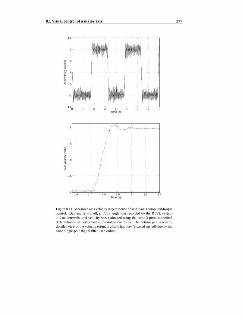
8.1Visual control of a major axis 277
0 1 2 3 4 5 6 7 8-1.5
-1
-0.5
0
0.5
1
1.5
Time (s)
Axi
s ve
loci
ty (
radl
/s)
1.6 1.7 1.8 1.9 2 2.1 2.2-1
-0.5
0
0.5
1
Time (s)
Axi
s ve
loci
ty (
radl
/s)
Figure8.11:Measuredaxisvelocitystepresponseof single-axiscomputed-torquecontrol. Demandis 1radl s. Joint anglewasrecordedby the RTVL systemat 2ms intervals, andvelocity wasestimatedusingthe same3-point numericaldifferentiationasperformedin theonline controller. The bottomplot is a moredetailedview of thevelocityestimateafterit hasbeen'cleanedup' off-line by thesamesingle-poledigital filter usedonline.

278 Further experimentsin visual servoing
0 0.1 0.2 0.3 0.4 0.5 0.6 0.7 0.80
0.2
0.4
0.6
Time (s)
j1 (
radl
)
0 0.1 0.2 0.3 0.4 0.5 0.6 0.7 0.8-3
-2
-1
0
1
Time (s)
j1d
(rad
l/s)
Figure 8.12: Measuredaxis responseof single-axiscomputed-torquecontrolshowing axispositionandvelocity: measured(solid) anddemand(dotted).Jointanglewasrecordedby the RTVL systemat 2ms intervals, andan off-line pro-cedureusing5-pointnumericaldifferentiationwasusedto obtainthe'measured'velocitydata.Theaxishasovershotandstopped0.005radlshortof thetarget.
used,giving a filter bandwidthof 13Hz. Thebottomplot in Figure8.11is a filteredversionfrom whichit canbeseenthatthereis veryslightovershootanda risetimeofaround0.1s leadingto a bandwidthestimateof approximately5Hz.
Figure8.12showstheperformanceof thecomputed-torquecontrollerfor thestan-dard0.5s swingtrajectory. Thecomputedtorquecontroller(8.35)andthetrajectorygenerator(8.1), (8.7)and(8.8)areexecutedevery 2ms. Thecontrolgainshave beensetempiricallyso asto achieve goodtrajectoryfollowing with minimum overshoot.Thereis againevidenceof velocity saturationbut at a higherspeedthanfor theUni-mate's native velocity controller. The final valueof the joint angleis lessthanthedemandsincetheaxishasovershotandstoppeddueto stiction.For over-dampedmo-tion, stictionwould stoptherobotshortof its target. Increasedproportionalgain,Kp,would reducethis errorbut is limited in practiceby stability criteria. IncreasingbothKp andKv leadsto roughmotiondueto noiseonthevelocityestimate.Integralactionwasexperimentedwith, but it wasdifficult to achievebothstabilityandaccuratetargetsettling.
Comparedto the native Unimatepositionandvelocity loops this controllerhas

8.1Visual control of a major axis 279
Characteristic Unimate Computed-torquesamplerate positionloop at 1ms in-
tervalpositionloop at 2ms in-terval
velocity estimation analog synthesis fromencoder signals withconsiderable low fre-quency gainboostduetolow-passfilter
digital estimation fromencodersignals at 2msinterval
integralaction analogimplementation digital implementationat2msinterval
Table8.2: Comparisonof implementationaldifferencesbetweenthenative Uni-matecontrollerandcomputed-torquecontrollerimplemented.
inferior low-speedperformance,particularlyin termsof achieving thetargetposition.Thesignificantimplementationaldifferencesbetweenthetwo controllersaresumma-rizedin Table8.2. A numberof papers[162,247]have examinedtheperformanceofPumacomputed-torquecontrollersbut the performancemetric usedis alwayshigh-speedtrajectoryfollowing error. Apart from noting this issueit will not bepursuedfurthersincetheexperimentis concernedprimarily with high-speedmotion.
The few narrow spikeson the velocity estimatearedueto timing jitter, that is,non-uniformtime stepsin samplingthe axis position. They arepresenteven duringmotion with no velocity feedback.Statisticsshow the standarddeviation in sampletiming is generally0.1msor 5%of thesampleinterval. In someinstancesthetimingjitter is moreseveredueto otheractivity underthereal-timeoperatingsystemsuchasinterruptlevel processing.Firstattemptsatcontrolusingthishighsamplerateyieldedvelocity plotswith a markedoscillationat approximately75Hz. Investigationof thisphenomenonshowed it to be due to interactionbetweenthe 2ms computed-torqueprocessrequestingtheaxispositionandthe984µsprocessin theUnimateaxisservoboardwhich updatesthe internal16-bit softwareencoderregisterfrom thehardwareencodercounter. Thiswasovercomeby modifying theUnimateaxisfirmwaresothatwhenin currentcontrolmodeit will returnthe instantaneousencodervalue,not thatobtainedat thelastservo clock tick.
8.1.6 Vision basedcontrol
This sectionintroducesa hybrid visualcontrolstrategy capableof stoppingtherobotdirectly over a randomly-placedtarget. The first phaseof the motion is underthecontrolof thetrajectorygeneratoraspreviously. Oncethetargetcomesinto view thecentroiddatafrom theend-mountedcamerais usedto bring therobot to a stopoverthe target. The trajectorygeneratorandcomputedtorquecontrol law areexecuted

280 Further experimentsin visual servoing
0 0.1 0.2 0.3 0.4 0.5 0.6 0.7 0.8-0.2
0
0.2
0.4
0.6
Time (s)
j1 (
radl
)
0 0.1 0.2 0.3 0.4 0.5 0.6 0.7 0.8-3
-2
-1
0
1
Time (s)
j1d
(rad
l/s)
Figure8.13: Measuredaxis responseunderhybrid visual control showing po-sition andvelocity: measured(solid) andtrajectory-generatordemand(dotted).Notethattheaxispositionhassettledatanegativevaluein orderto movethema-nipulatoroverthetarget.Thesystemswitchedto visualservoingatapproximatelyt 0 4s.
at a 2ms interval asin theprevioussection,until the targetcomesinto view. Undervisual control thecentroidandcentroidvelocity areestimatedevery 20msandusedto computetheaxisvelocitydemand
θdiKp
iXdiX iKv
i ˆX (8.38)
usingasimplePDcontrollaw. Thecomputedtorquecontrolis still executedata 2msinterval but the axis positionerror andtrajectoryaccelerationfeedforwardtermsaredroppedgiving
τd M Kv θdˆθ F ˆθ (8.39)
whereKv hasthesamevalueaspreviously. Thegainsfor the visualservo loop, iKp
and iKv, weresetempiricallyandit waspossibleto achieve goodsteady-stateerrorperformancewith acceptableovershoot.Relatively high gainswerepossibleduetotheeffectivenessof thecomputed-torquevelocity loop. Onceagainthehigh level offriction wasa problemat low speed,andattemptsto achieve critical dampingled tothe robot stoppingshortof the target. The additionof an integral term to (8.38) is

8.1Visual control of a major axis 281
0.35 0.4 0.45 0.5 0.55 0.6 0.65 0.7 0.75
0
20
40
60
80
100
120
140
Time (s)
Tip
dis
plac
emen
t (m
m)
Figure8.14: Measuredtip displacementdeterminedfrom end-effectormountedcamerafor hybridvisualcontrolstrategy.
helpful in the longerterm in bringingthe robot to the destination,but high levelsofintegralgainagainleadto oscillatorybehaviour.
Figure8.13showsa typical trajectoryfor a targetdisplacedapproximately20mmfrom thedestinationof thetrajectorygenerator. Theeffectof thisdisplacementcanbeseenin thefinal valueof thejoint anglewhichis -0.0884radlratherthanthetrajectorygeneratordemandof 0radl. Thetargetcomesinto view at 0.32s andthetransitionincontrolstrategiesoccurred4 field timeslaterat approximately0.40s. The transitionis smooth,helpedby theaxisbeingvelocity-limitedat thatpoint. Figure8.14showstheend-pointerrorsensedby thecamerascaledinto lengthunits. Theend-pointhasfollowedanalmostcritically dampedtrajectoryandby 0.60stheend-pointhassettledto within 1pixel or 0.78mmof thetargetwhosepositionwasunknown.
8.1.7 Discussion
Thissectionhasprovideda preliminaryinvestigationinto someof theissuesinvolvedin thecontrol,usingvision andaxisfeedback,of a realisticrobotaxis. Theaxischo-senhasa numberof seriousnon-idealitiesthat includeresonanceandhigh levelsofstiction, viscousandCoulombfriction. A high-bandwidthvelocity loop wasimple-mentedusinga single-axiscomputed-torquecontrollerwith velocity estimatedfrom

282 Further experimentsin visual servoing
measuredaxisposition.Althoughthewrist axescouldbevelocity-controlledat50Hz,this axishasa numberof resonancesup to 45Hz whichseriouslylimit theachievableclosed-loopperformance.Thedynamicsof thestick-slipandCoulombfriction effectalsohave very shorttime constantsrequiringa high samplerate.Thedigital velocityloop wasrun at 500Hz andprovided high-qualityvelocity control for the overlyingtrajectorygeneratoror visualfeedbackloop.
A challengingtrajectorywaschosenat the performancelimit of the robot. TheUnimateaxis controller, with its lower velocity capability, wasunableto follow thetrajectoryandaccumulatedincreasingpositionerror. As theaxisapproachedthedes-tinationit deceleratedvery rapidly, therebyexciting structuralresonancesin thearm.Theseresonancescouldbedetectedby anaccelerometermountedon thecameraandalsoby theireffectonthemotor'stransferfunction.This lattereffectcauseddifficultywith a 50Hz digital velocity loopandthesampleratehadto beraisedto 500Hz. Thecomputed-torquecontrollerwasable to achieve a morerapid responsewith similarovershoot,but wasmoreproneto stiction andcurrentlyhaspoor low-speedmotioncapability. Thehybridcontroller, usingvisualfeedbackfor final positioning,wasableto reliably positionthe robot to within 1 pixel of the centroidof a randomlyplacedtarget.
Interestinglythevisualloop,despiteits low samplerate,wasseeminglyunaffectedby thestructuralresonance.This is partly dueto the low displacementamplitudeofthe oscillation. In the exampleof Section8.1.3the peakamplitudeis only 1mm orapproximately1.3pixelsdespitethesignificantaxis accelerationstep. Closeinspec-tion of the visually sensedtip displacementin Figure8.5 shows no evidenceof thisoscillation,whichwill bemaskedby themotionblur effectdiscussedin Section3.5.6.
Visual servoing is likely to be most useful in controlling manipulatorsthat areeithervery rigid or, moreinterestingly, lessstiff (andhencecheaper)with vibrationsoccurringwell below theNyquist frequency andthusamenableto visualclosed-loopendpointcontrol. The latter is quite feasible,with the bandwidthachievablelimitedprimarily by thesamplerateof thevisualsensor. Cannon[42] observesthatcontrolofthemanipulator'send-pointusinga non-colocatedsensorcomplicatescontroldesign,but canresultin superiorperformance.UnfortunatelythePumarobotavailablefor thiswork is moredifficult to control, sincesignificantresonancesexist on eithersideoftheNyquist frequency, eventhoughtherobotposewasselectedin orderto minimizethosefrequencies.
8.2 High-performance3Dtranslational visualservoing
This sectiondescribesanexperimentin high-performancetranslationalvisual servo-ing. Threerobot DOF arecontrolledby imagefeaturesso asto keepthe cameraata constantheightvertically above a target rotating on a turntable. A plan view isshown in Figure8.15. The controllerwill usevisual feedforwardof target velocity

8.2High-performance3D translational visual servoing 283
XcYc
turntable
two target markers
Figure8.15:Planview of theexperimentalsetupfor translationalvisualservoing.
andcomputed-torqueaxisvelocity-controlloopssinceaxisinteractiontorquesareex-pectedto besignificantat theanticipatedjoint speedsandaccelerations.
8.2.1 Visual control strategy
In orderto control3 robotDOF werequire3 'pieces'of informationfrom theimage.As in previousexamplesthecentroidgivesanX andY targetdisplacementwith re-spectto thecameraandtheextra informationrequiredis targetdistance.From(3.66),for theX-axis,wecanwrite
cxt
cz fαx f
iX X0 (8.40)
which givestheestimatedtargetpositionrelative to thecamerain termsof theimageplanecoordinateandtarget distance.A similar expressioncanbewritten for theY-axis.Thecameracoordinateframecanbedeterminedfrom measuredjoint anglesandforwardkinematics
0Tc K θ t6Tc (8.41)
which providesthe cameraposein world coordinatesallowing the target positioninworld coordinatesto beestimated
0xt0Tc
cxt (8.42)
wherecxtcxt
cytczt .

284 Further experimentsin visual servoing
The remainingproblemis estimationof targetdistance,czt , which is requiredtocontrol the robot's Z-axis Cartesianmotion andis also requiredin (8.40). Using amonocularview theapproachesto distanceestimationareratherlimited. Stadimetryis asimpletechniquebasedontheapparentsizeof theobjectbut is sensitiveto changesin lighting level andthresholdasdiscussedin Section4.1.3.4.A morerobustapproachis basedon the distancebetweenthe centroidsof two featuressincecentroidwaspreviouslyshown to berobustwith respectto lighting andthreshold.Considerascenewith two circularmarkerswheretheX andY imageplanecomponentsof thecentroiddifferenceare
i∆XiX1
iX2i∆Y
iY1iY2 (8.43)
TheX andY axeshave differentpixel scalefactors,seeTable3.8,so thesedisplace-mentsmustbescaledto lengthunits
∆x
czti∆X
αx f∆y
czti∆Y
αy f(8.44)
Thedistancebetweenthecentersof themarkers
∆ ∆2x ∆2
y (8.45)
is known, allowing anexpressionfor rangeto bewritten
cztf ∆
i∆2X
αx
2 i∆2Y
αx
2(8.46)
The centroidusedfor fixation purposesis the meancentroidof the two circlefeatures.Thetargetpositionestimatesin theworld framearegivenby (8.42)andtheX andY componentsareinputto trackingfiltersin orderto estimatethetarget'sworld-frameCartesianvelocity, 0ˆxt . Thisprovidesthevelocityfeedforwardcomponentof therobot's motion. The feedbackCartesianvelocity componentis derivedfrom image-planecentroiderrorandestimatedtargetrangeerror
cxeiKp
iXdiX iKv
i ˆX (8.47)cye
iKpiYd
iY iKvi ˆY (8.48)
cze Kzczt
czd (8.49)
As shown in Figure8.16thetwo velocity componentsaresummedin thewrist refer-enceframe
t6xdt6J0
0ˆxt
feedforward
t6Jccxe
feedback
(8.50)

8.2High-performance3D translational visual servoing 285
θ.d
+ Xi
d
Xi
-
Xi
1
z
R z( )
xt z( )robot
+
+
x0
tx.0
t
τc
B
Kv
Jt6
c
Jt6 1−
θM
3-pt velestim
3-pt velestim
PI
κ θ( )
+
+
+
+
xc
t
T0
c
θ
θ.
θ.θ
zc
d
-+
zc
+
+
x.t6
d
N
4ms
40ms
20ms
lens,sensor,vis.sys
targetposn.estim.
depth
dyn.coeff.
trackingfilter
velocityfeedforward
velocityfeedback
+ +
x.c
dx.t6
d
J6
0
x.t6
t
τd
x
estim
Figure8.16:Block diagramof translationalcontrolstructure.
The camera-mountJacobian,t6Jc, is a constantand is determined(from t6Tc givenearlierin (4.73))using(2.10)to be
t6JccJ 1
t6
1 0 00 0 10 1 0
(8.51)
andinvolvesonly transpositionsandsignchanging.TheotherJacobian,t6J0, is con-figurationdependentanddeterminedonline using(2.10)andthe currentestimateof0Tt6.
In thefinal stepthetotalCartesianvelocitydemandis resolvedto joint velocitybythemanipulatorJacobian
θdt6Jθ θ 1t6xd (8.52)
to provide theaxis velocity demand.The inversemanipulatorJacobianis computedusingthemethodof Paul andZhang[202]. All Jacobiansin theabove equationsare3 3.

286 Further experimentsin visual servoing
8.2.2 Axis velocity control
High-performanceaxis velocity control will be requiredfor the robot's baseaxes,and from experiencein the previous sectiona high samplerate will be required.Computed-torquecontrolwill beusedto compensatefor rigid-bodydynamiceffectswhich areexpectedto be significantin this experiment. For online dynamicscom-putationit is desirableto divide thecomputationinto two components,oneexecutedat the axis servo rate andanother, generallycoefficient computation,executedat alower rate. Thereare two motivationsfor this. The first, which is widely men-tioned [149,201,228], is that this reducesthe amountof computationthat needbedoneat thehighsamplerateandthussignificantlylowerstheburdenontheprocessor.Secondly, Sharkey et al. [228] suggestthat it maybecounter-productive to computejoint torquesat a high-ratebasedona dynamicmodelthatdoesnot takeinto accounthigher-ordermanipulatordynamiceffects. The RNE proceduredescribedearlier inSection2.2.2computestorqueasa functionof θ, θ and θ andsuffers the objectionsjust mentionedwhencomputedat thehighsamplerate.
In reportsof controllersusing this dual-rateapproach[149,228] the coefficientmatrices,M , C, andG arecomputedat a low ratewhile the torqueequation(2.11)is executedat the higher samplerate. However this raisesthe questionof how tocalculatethesecoefficient matrices.Symbolicalgebraapproachescouldbeusedbutthe run-time computationalcostmay be significantsincethe efficient factorizationof theRNE procedurecannotbeexploited.Armstrongetal. [20] provideclosed-formexpressionsfor thecoefficientmatricesderivedby symbolicanalysisandsignificance-basedsimplification;however thekinematicconventionsaredifferentto thoseusedinthiswork. Instead,theapproachtakenwasto begin with thesymbolicsum-of-producttorqueexpressionsdevelopedearlierandapplytheculling procedureof Section2.6.3to automaticallyeliminatetermsbelow 1% significance.Theexpressionswerethensymbolicallypartitioned
τ M θ θ N θ θ (8.53)
whereM is the3 3manipulatorinertiamatrixandN is a3-vectorcomprisinglumpedgravity, centripetalandCoriolis torques.GivencoefficientsM andN equation(8.53)canbeevaluatedwith only 9 multiplicationsand9 additionsresultingin a very lowcomputationalburdenof only 81µs. The coefficients M andN, updatedat 25Hz,arecomputedby a MAPLE generated'C' function that takes1.5msto execute.Thelow rateof coefficient updateis not a problemin this situationsincetheposecannotchangesignificantlyover the interval, andaxis velocity can be assumedpiecewiseconstantsincethedemandis only updatedat thevideosamplerateof 50Hz.
Evaluatingthecoefficientsfrom theexpandedtorqueequationis computationallylessefficient thantheRNEalgorithm.However thisapproachallowsthecomputationto be partitionedinto a 'lightweight' componentfor executionat a high servo rateanda moderatelymoreexpensive componentto executeat a lower samplerate. The

8.2High-performance3D translational visual servoing 287
computationalburdencanbeexpressedasthefraction
executiontimeperiod
Computingthe3-axisRNE (symbolicallysimplified)at 4ms(usingtiming datafromTable2.25)resultsin a burdenof
7804000
20%
while thedual-rateapproachhastwo, relatively small,components
814000
150040000
6%
totalling lessthan one third the burdenof the straightforwardRNE. The dual-rateapproachalsosatisfiestheproblemof unwantedcouplingof unmodelledmanipulatordynamics.
Thevelocitycontroller, evaluatedatthe4msperiod,usessimpleproportionalgain
τd MK v θdˆθ N F ˆθ (8.54)
andfriction compensationasdescribedin theprevioussection.M andN areupdatedat a40msinterval.
8.2.3 Implementation details
To implementthiscontrolstrategy underVxWorksandRTVL anumberof concurrentcommunicatingtasks,shown in Figure8.17,areused:
field is a high-priority taskthat samplesthe joint anglesinto the sharedvariablej6 vis at thebeginningof verticalblanking.It thenactivatesthecentroid ,viskine anddynpar tasks.
viskine is a 20ms periodictaskthat computesthe cameracoordinateframeoTc
andtheinversemanipulatorJacobiant6Jθ from currentjoint anglesj6 vis .
centroid is a20msperiodictaskthatprocessesregiondata,estimatestargetrangeby (8.46),Cartesianvelocityby (8.47)- (8.50),whicharethenresolvedto jointratedemandsandwritten to thd d.
torque is a4msperiodictaskthatperformsthecomputed-torqueaxisvelocity loopcalculationsfor joints1 to 3.

288 Further experimentsin visual servoing
field viskine
centroid
dynpar
torquecamera
j6_cur
j6_vis
tracking filterstate
thd_d
M, N
Jc
Visionhardware
videofieldinterrupt
encoderscurrentdemand
position demandjoint 5
Robot hardware interface to Unimate AIB
pendant
Figure 8.17: Task structurefor translationcontrol. Arrows representdataflow,lighting boltsareevents,ellipsesaretasksand'3D' boxesaredatastructures.
dynpar is a 40msperiodictaskthat updatesthe rigid-body coefficientsM andNbasedon current joint anglesand velocity estimatedover the last threetimestepsusinga3-pointderivative.
camera is a 7msperiodictaskthat is responsiblefor keepingthe camera's opticalaxisnormalto themotionplane.Motion of the lower threejoints changestheorientationof thecamerawhich this taskcountersby appropriatewrist motion.

8.2High-performance3D translational visual servoing 289
θ2
−θ3
θ5
Figure8.18: Cameraorientationgeometry. Thecameracanbemaintainednormalto theworkingsurfaceif θ5 θ2 θ3 π .
Function Period Executiontimeµs µs % of CPU
torque 4000 1844 46viskine 20,000 3800 19dynpar 40,000 1500 4centroid 20,000 1300 7Total 76
Table8.3: Summaryof taskexecutiontimes. Theseareaverageelapsedtimesforexecutionof codesegmentsandnoallowancehasbeenmadefor theeffectsof taskpreemptionduringexecution.
Fromthesimplegeometrydepictedin Figure8.18it is clearthatcompensationcanbeachievedby motionof asinglewrist axis
θ5 θ2 θ3 π (8.55)
pendant is a low-priority continuoustaskthatcommunicateswith the robot teachpendantusing the ARCL pendantcommunicationprimitives. Several modesof operationcanbe selectedby the teachpendantand includevisual fixationcontrol,manualjoint velocity controlandmanualCartesianvelocitycontrol.
Execution times of the variousmodulesare summarizedin Table 8.3 in abso-lute termsandas a fraction of total computingburden. The torquetaskconsumes

290 Further experimentsin visual servoing
the largest fraction, but a good dealof that time is takenup with communicationsoverhead:680µs to readthethreeencoders,and510µs to transmitthemotorcurrentdemands.Velocity estimation,computedtorquecomputation,friction compensationandcurrentclipping takeonly 220µs axis. Thesecomputationsaccountfor 76%ofthe computationalresource,and additionalprocessingis requiredfor datalogging,userinterface,graphicsandnetworking. Clearly the processor, in this casea single33MHz 68030,is closeto its limit.
8.2.4 Resultsand discussion
Thetrackingperformanceof thecontrollerfor thestandardtargetmotionis shown inFigure8.19.Theerrormagnitudein theY directionis similar to thatdisplayedby the2-DOFpan/tilt controllerof Section7.5. Thecentroiderror is significantlygreaterintheX directionthantheY directionandthis is believedto bedueto thepoordynamicperformanceof thewaistaxis. Performanceof thataxisis limited by significantfric-tion andtherelatively low velocitygainneededto ensurestability. Figure8.20showstheresultsof thesameexperimentbut with centripetalandCoriolis feedforwarddis-abled. Clearly the Y-axis trackingperformanceis substantiallydegradedwith onlypartialcompensationof manipulatorrigid-bodydynamiceffects.Disablingtargetve-locity feedforwardresultsin verypoorperformance,andit is notpossibleto keepthetarget in the camera's field of view even at 20% of the velocity demonstratedhere.Themanipulatorjoint ratesshown in Figure8.21peakat approximatelyhalf thefun-damentalmaximumjoint ratesestablishedin Table2.21.At thepeakvelocity thereissometendency towardoscillation,particularlyfor joints1 and2.
The loggedjoint angletrajectorydatawastransformedoff-line by themanipula-tor forwardkinematicsto determinethecamera's Cartesiantrajectorywhichis shownin Figure8.22. Thecamera's height,cz, is not constantandhasa peak-to-peakam-plitude of approximately40mm. This performanceis dueto the relatively low gainproportionalcontrolstrategy (8.49)usedfor thisDOF. TheCartesiancameravelocityis shown in Figure8.23alongwith the online estimatedtarget velocity. The veloc-ity feedforwardsignalis a goodestimateof the actualtarget velocity. The peaktipspeedis 350mm sandthis is approximatelyonethird of themanufacturer'sspecifiedmaximum.Therobotappearedto be'working hard' andwith considerablegearnoise.
The Cartesianpathof the camera,shown in Figure8.24, is only approximatelya circle andtwo factorscontribute to this distortion. Firstly, non-idealtrackingper-formancecausesthe camerato deviate from the path of the target. Secondly, thecamerais not maintainedin anorientationnormalto theXY plane.Thecontributionof thesetwo effectscanbe understoodby looking at the online target positionesti-mates. Thesearecomputedfrom target centroidand joint angledataandmakenoassumptionsabouttrackingperformance.Figure8.25showsthisestimatedtargetpathwhich is clearlydistortedlike thepathactuallyfollowedby thecamera.Similarplots,

8.2High-performance3D translational visual servoing 291
0 1 2 3 4 5 6 7 8 9-50
0
50
Time (s)
Y e
rror
(pi
xels
)0 1 2 3 4 5 6 7 8 9
-50
0
50
Time (s)
X e
rror
(pi
xels
)
Figure8.19: Measuredcentroiderror for translationalvisual servo controlwithestimatedtargetvelocityfeedforward.RMSpixel erroris 28and7.3pixelsfor theX andY directionsrespectively.
0 1 2 3 4 5 6 7 8 9-50
0
50
Time (s)
Y e
rror
(pi
xels
)
0 1 2 3 4 5 6 7 8 9-50
0
50
Time (s)
X e
rror
(pi
xels
)
Figure8.20: Measuredcentroiderror for translationalvisual servo controlwithestimatedtarget velocity feedforward,but without centripetalandCoriolis feed-forward. RMS pixel error is 30 and22pixels for theX andY directionsrespec-tively.

292 Further experimentsin visual servoing
1 2 3 4 5 6 7 8 9
-1
0
1
Time (s)
j3d
1 2 3 4 5 6 7 8 9
-0.5
0
0.5
Time (s)
j2d
1 2 3 4 5 6 7 8 9-0.5
0
0.5
Time (s)
j1d
Figure8.21: Measuredjoint rates(radl/s) for translationalvisual servo controlwith estimatedtargetvelocity feedforward.Velocity is estimatedoff-line usinga5-pointnumericalderivativeof joint anglesmeasuredby RTVL.
but for significantlylower cameraspeed,arealmostidealcircles.At thejoint speedsusedin this experimentthe wrist axes,undercontrol of the Unimatepositionloops,areunableto accuratelytrackthewrist orientationdemand(8.55).Fromtherecordeddatait appearsthattheactualθ5 lagsthedemandby approximately21msresultinginpeak-to-peakorientationerrorsof 0.043radlandthis is verifiedusingtheSIMULINKmodelof Figure2.26.In addition,dynamicforcesactingonthecameraresultin smallrotationsof joints4 and6. Theseseeminglysmallorientationerrors,coupledwith thenominal500mmtargetdistance,resultin considerabletranslationalerrors.
It is interestingto contrastthe control structurejust describedwith someotherstructuresdescribedin the literature.Operationalspacecontrol,proposedby Khatib[149], wouldappearto beanidealcandidatefor suchanapplicationsincea cameraisanoperational(or task)spacesensor. In factanexampleof visionbasedcontrolusingtheoperationalspaceformulationhasbeenrecentlydescribedby Woodfill etal. [284].Operationalspacecontrol transformsthe robot andsensordatainto the operationalspacewheredegreesof freedomcanbe selectedaspositionor force controlledanddesiredmanipulatorend-pointforcesarecomputed. Finally theseforcesare trans-formedto joint spaceandactuatethemanipulator. As expressedin Khatib [149] the

8.2High-performance3D translational visual servoing 293
0 1 2 3 4 5 6 7 8 9600
800
Time (s)
Xc
0 1 2 3 4 5 6 7 8 9
-200
-100
Time (s)
Yc
0 1 2 3 4 5 6 7 8 9
120
140
Time (s)
Zc
Figure8.22: MeasuredcameraCartesianposition(mm) for translationalvisualservo control with estimatedtarget velocity feedforward.Cartesianpathdataisestimatedoff-line from joint angles(measuredby RTVL) usingforwardmanipu-lator kinematics.
0 1 2 3 4 5 6 7 8 9-400
-200
0
200
400
Time (s)
Xd
(mm
/s)
0 1 2 3 4 5 6 7 8 9-400
-200
0
200
400
Time (s)
Yd
(mm
/s)
Figure8.23: MeasuredcameraCartesianvelocity (solid) with estimatedtargetvelocity feedforward(dashed).Cameravelocity is estimatedoff-line usinga 5-pointnumericalderivativeof theCartesianpositiondataof Figure8.22.

294 Further experimentsin visual servoing
manipulatortorqueloop is closedat a rateof 200Hz which is likely to bedictatedbycomputationallimits. If a machinevision sensoris usedthenthe torqueloop wouldbeclosedat a maximumof 60Hz (assumingRS170video)which hasbeenshown tobetoo low to achieve high-performancefrom thenon-idealPumaaxes.Thestructureproposedin this sectionis hierarchicalandmore appropriatefor the caseof a lowsampleratesensorsuchasamachinevisionsystem.
8.3 Conclusion
This chapterhasextendedandbroughttogethermany of theprinciplesestablishedinearlierchaptersby meansof two examples:1-DOF visual control of a major robotaxis,and3-DOFtranslationalcameracontrol. Thesimple2-DOFcontrolof thepre-viouschaptereffectively decoupledthedynamicsof eachaxis,with oneactuatorpercameraDOF. In the3-DOFtranslationalcasethereis considerablekinematicanddy-namic couplingbetweenthe axes involved. To achieve high-performancetrackinga multi-ratehierarchicalcontrolsystemwasdeveloped.Target velocity feedforwardwasfound to be essentialfor the accuratetrackingat high speedshown in Section8.2. Feedforwardof manipulatorrigid-bodydynamics,that is computed-torquecon-trol, hasalsobeenshown to increasethe trackingaccuracy. The end-pointcontrolexperimentof Section8.1 did not usevisual feedforward,but in thatcasethe targetwasstationaryandthemanipulatorwasdecelerating.
The controllercomputationalhardware,which hasserved well over a periodofmany years,is now at thelimit of its capability. Workingin suchasituationis increas-ingly difficult andunproductiveandprecludestheinvestigationof moresophisticatedcontrolstructures.Theactof enablingdataloggingfor theexperimentof Section8.2now causesa visibledegradationin performancedueto increasedlatenciesandviola-tionsof designedtiming relationships.Theexperimentalfacility hashowever demon-stratedthatsophisticatedcontroltechniquesincorporatingmachinevision,rigid-bodydynamicsandfriction compensationcanbeachievedusingonly asingle,modest,pro-cessor.

8.3Conclusion 295
550 600 650 700 750 800 850
-200
-150
-100
-50
Xc (mm)
Yc
(mm
)
Figure8.24: MeasuredcameraCartesianpath in the XY plane. CartesianpathdataasperFigure8.22.
550 600 650 700 750 800 850-250
-200
-150
-100
-50
0
Figure8.25:MeasuredcameraCartesianpathestimatefrom onlinetrackingfilterrecordedby RTVL.

296 Further experimentsin visual servoing

Chapter 9
Discussionand futur e dir ections
9.1 Discussion
This bookhaspresentedfor thefirst time a detailedinvestigationof themany facetsof a robotic visual servoing systemwith particularemphasison dynamiccharacter-istics and high-performancemotion control. The useof machinevision for high-performancemotioncontrolis asignificantchallengedueto theinnatecharacteristicsof thevisionsensorwhichincluderelatively low samplerate,latency andcoarsequan-tization.
A distinction has beenestablishedbetweenvisual servo kinematicsand visualservo dynamics. Theformeris well addressedin theliteratureandis concernedwithhow themanipulatorshouldmove in responseto perceivedvisualfeatures.Thelatteris concernedwith dynamiceffects due to the manipulatorandmachinevision sen-sorwhich mustbeexplicitly addressedin orderto achieve high-performancecontrol.This problemis genericto all visually controlledmachinesno matterwhatapproachis takento featureextractionor solvingthevisualkinematicproblem.
Weissproposeda robotcontrolschemethatentirelydoesaway with axissensors— dynamicsandkinematicsarecontrolledadaptively basedon visual featuredata.This concepthasa certainappealbut in practiceis overly complex to implementandappearsto lackrobustness.Theconceptshaveonly everbeendemonstratedin simula-tion for up to 3-DOFandthenwith simplisticmodelsof axisdynamicswhich ignore'realworld' effectssuchasCoulombfriction andstiction. However theusefulnessofsucha controlapproachis opento question.It is likely that robotswill alwayshaveaxispositionand/orvelocity sensorssincenot all motionwill be,or canbe,visuallyguided. Ignoring thesesensorsaddsgreatlyto the control complexity andhasbeenshown to lead to inferior control performance.Structuralresonancesand the timeconstantsof stick-slipfriction, ignoredby Weiss,dictateasampleinterval of lessthan
297

298 Discussionand futur e dir ections
4ms,which is not currentlyachievablewith off-the-shelfvideoor imageprocessingcomponents.If constrainedby thevisionsystemto low samplerates,high-bandwidthaxis level feedbackis requiredfor high-performanceandrobustcontrol. Axis posi-tion andvelocity informationarealsoessentialfor model-baseddynamiccontrolandJacobiancomputation.
In orderto overcomelow visualsampleratessomeresearchershave proposedtheuseof trajectorygeneratorsthatcontinuouslymodify theirgoalbasedonvisualinput.In this bookthe taskhasinsteadbeenconsideredasa 'steeringproblem',controllingthe robot's velocity so as to guide it toward the goal. Conceptuallythis leadsto avisual position loop closedaroundaxis velocity loops. This structureis analogousto thecommonrobotcontrolstructure,exceptthatpositionis senseddirectly in taskspaceratherthanjoint space.
Theterm'high performance'hasbeenwidely usedin thisbookandwasdefinedattheoutsetasrobotmotionwhichapproachesor exceedstheperformancelimits statedby the manufacturer. The limits for the robot usedwereestablishedin Chapter2.Thereis alsoan implied fidelity criterion which wasdefinedlater in termsof pixelerrorfor trackingapplications.
The performanceachieved is a consequenceof the detailedunderstandingof thedynamicsof the systemto be controlled(the robot) andthe sensor(the cameraandvision system).Despitethe long history of researchin theseareasindividually, andcombinedin visualservoing,it is apparentthatmuchof thedatarequiredfor modellingis incompleteandspreadthrougha verydiverseliterature.Thisbookhasattemptedtodraw togetherthis disparateinformationandpresentit in a systematicandconsistentmanner.
A numberof differentcontrol structureshave beendemonstratedin experimentsandsimulation.Feedback-onlycontrollerswereshown to becapableof high perfor-mancebut werefoundto berather'brittle' with respectto actuatorsaturation.Theirdesignwas alsofound to be seriouslyconstrainedin order to achieve compensatorstability which hasbeenshown to be important. Feedforwardincreasesthe designdegreesof freedomand a control strategy basedon estimatedtarget velocity feed-forwardwasintroduced.With no a priori knowledgeof targetmotion thecontrollerdemonstratessufficientperformanceto fixateonanobjectrotatingona turntableor aping-pongball thrown in front of therobot.
Thekey conclusionsfrom this work arethatin orderto achieve high-performancevisual servoing it is necessaryto minimize open-looplatency, have an accuratedy-namicmodelof the systemandto employa feedforwardtypecontrol strategy. Pre-dictioncanbeusedto overcomelatency but at theexpenseof reducedhigh frequencydisturbancerejection. Open-looplatency is reducedby choiceof a suitablecontrolarchitecture.An accuratedynamicmodelis requiredfor controlsynthesis.Feedback-only controllershave a loop gain limit dueto thesignificantdelayin pixel transportandprocessing.Simplefeedbackcontrollershave significantphaselagcharacteristics

9.2Visual servoing: somequestions(and answers) 299
which leadto poor tracking. More sophisticatedfeedbackcontrollerscanovercomethis but the solutionspacebecomesvery constrainedandthe controllersarenot ro-bustwith respectto plantparametervariation.Feedforwardcontrolresultsin a robustcontrollerwith excellenttrackingcapability.
9.2 Visual servoing: somequestions(and answers)
Thissectionposesanumberof pertinentquestionsthatwereposedattheoutsetof theoriginalPhDresearchprogram.They areworthrepeatinghere,alongwith answersintermsof materialcoveredin this book,sincethey providea succinctencapsulationofthemajorconclusionsof this research.
1. Canmachinevisionbeusedtocontrol robotmanipulatorsfor dynamicallychal-lenging tasks,by providing end-pointrelative sensing? Machinevision andend-pointsensingcanbeusedfor dynamicallychallengingtasksif thegeneralprinciplessummarizedabove areobserved. Thelimits to visualservo dynamicperformancehave beeninvestigatedandsuitablecontrol structureshave beenexploredby analysis,simulationandexperiment.Commonlyusedperformancemeasuressuchasstepresponsehave beenshown to beinadequatefor thegen-eraltargettrackingproblem.Alternativemeasures,basedon imageplaneerror,have beenproposedto enablemoremeaningfulcomparisonof results.
2. Whatare thelimiting factorsin imageacquisitionandprocessing?Theseissueswereaddressedprincipally in Chapter3. Imagefeatureextraction,by special-izedhardwareor evensoftware,is now easilycapableof 50or 60Hz operation,andthefundamentallimit to visualservo performanceis now thesensorframerate. It hasbeenshown that the requirementsfor ideal visual samplingandreducingmotionblur requireshortexposuretimes,andconsequentlyconsider-ablesceneillumination, which maybe a problemin someapplicationsduetothe heatgenerated.At higherframerates,andin order to maintainthe idealsamplerapproximation,evenshorterexposuretimeswould berequired,neces-sitating increasedillumination or moresensitive sensors.A camera-mountedpulsed-LEDlighting systemhasbeendemonstratedthat provides light whenandwhererequired.
More robustsceneinterpretationis definitely requiredif visually servoedsys-temsare to move out of environmentslined with black velvet. Optical flowbasedapproachesshow promise,and have beendemonstratedat 60Hz withspecializedprocessinghardware.
Maintainingadequatefocusis often consideredimportantfor visual servoingandis difficult to achieve givenvariationin relative target distance.The lenssystemmaybeconfiguredfor largedepthof fieldbut thisfurtherexacerbatesthe

300 Discussionand futur e dir ections
lighting problemsjust mentioned.Theupperboundon imageclarity hasbeenshown to bedeterminedby effectssuchaslensaberrationandto a lesserextentpixel re-sampling.It hasalsobeenshown thatbinary imageprocessingin thepresenceof edgegradientsresultsin featurewidth estimatesthatarefunctionsof thresholdandoverall illumination, but thatcentroidestimatesareunbiased.For imageprocessingapproachesbasedonedgesor texture,for instanceopticalflow or interestoperators,imageclarity wouldbeimportant.
3. How cantheinformationprovidedby machinevisionbeusedto determinetheposeof objectswith respectto the robot? This is what hasbeentermedinthis book the kinematicsof visual control and a numberof techniqueswerereviewed in Chapter4. This problemis solved for all practicalpurposes,andthe computationalcostsof thevariousproposedapproaches,imagebasedandpositionbased,arecomparableandreadilyachieved.Controlof a6-DOFrobotwasdemonstratedby Ganapathy[98] adecadeagousingaclosed-formsolutionthatexecutedin only 4msona68000processor. An iterativeapproachhasevenbeenpatented[289].
Theimage-basedtechniquehasbeendemonstratedto work well, but theadvan-tagesseemillusory, andthe problemof imagefeatureJacobianupdatein thegeneralcaseremains,althoughadaptationandgenerallearningschemeshavebeendemonstrated.The 3-D sceneinterpretationproblemcan be easedsig-nificantly by using3-D sensors.Sensorsbasedon structuredlighting arenowcompactandfastenoughto usefor visualservoing.
4. Can robot tasksbespecifiedin termsof what is seen?For a large numberofrobotic tasksthe answeris clearly 'yes' but this book hasprovided only par-tial answersto the question.A numberof papersreviewed in Chapter4 havediscussedhow taskscanbedescribedin termsof imagefeaturesanddesiredtra-jectoriesof thosefeaturesbut mostof thesystemsdescribedaresinglepurpose.Thereappearsto havebeenlittle work on languagesfor generalspecificationofvisually servoedtasks. In a semi-automatedsituationsuchastime delaytele-operationan operatormay be ableto selectimagefeaturesand indicatetheirdesiredconfigurationandhave the executionperformedunderremoteclosed-loopvisualcontrol.Therearesomereportson this topic [198].
5. Whateffectsdorobotelectro-mechanicalandmachinevisiondynamicshaveonclosed-loopdynamicperformance?Thevision systemwasmodelledin detailin Section6.4whereit wasshown thatthedominantcharacteristicsweredelaydueto pixel transportandgaindueto lensperspective. Theeffective delaywasshown to dependon thecameraexposureperiod,andfor somevisualservoingconfigurationsthegainwasshown to dependon targetdistance.Both charac-teristicscanhave significanteffect onclosed-loopsystemstability.

9.2Visual servoing: somequestions(and answers) 301
In Section6.4 theelectro-mechanicaldynamicscouldberepresentedby a unitdelaydue to the actionof a positioncontrol loop. Whenthe axesareveloc-ity controlledthedynamicsarefirst-orderandtheeffective viscousdampingisstronglydependenton motionamplitudedueto theeffect of Coulombfriction.For visual servo controlof a major axis,asdescribedin Chapter8, additionaldynamiceffectssuchasstructuralresonanceandsignificantstictionareencoun-tered.
Structuraldynamicswerediscussedin Section8.1.4andare importantwhenthemanipulatorhassignificantstructuralor transmissioncompliance,andhighendpointaccelerationis required.Visualservoing,by providing directendpointpositionfeedback,canbeusedto controlendpointoscillation,Section8.1.Thismayonedaybea viablealternative to thecommonapproachof increasinglinkstiffnesswhichthennecessitateshighertorqueactuators.
6. Whatcontrol architecture is bestsuitedfor such anapplication?Many aspectsof the control architectureemployedin this work arevery well suitedto thistasksinceit providestheprerequisitesidentifiedin Section6.1,in particular:
a high-frame-ratelow-latency vision systemwhich reduceslatency to theminimumpossibleby overlappingpixel transportwith region extraction;
a high bandwidthcommunicationspath betweenthe vision systemandrobotcontrollerachievedby a sharedbackplane.
The control architecturehasevolved asshortcomingswere identified,andanobvious weaknessin the early work wasaddedlatency due to servo setpointdoublehandlingand the multi-rate control structure. In later work this waseliminatedby implementingcustomaxisvelocity loopswhich werealsocapa-ble of higherspeed. The greatestbottleneckin the architecturedescribedinthisbookis now thecommunicationslink to theUnimateservosandthedigitalservo boardsthemselves,particularlywhenimplementinghighsamplerateaxiscontrol.A moreappropriatearchitecturemayinvolvedirectmotorcontrolby adedicatedmotorcontrolcard,perhapsanotherVMEbusprocessor, anddispens-ing with theUnimatedigital servo board.A differentrobotmayalsoeliminatesomeof thesedifficulties.
Thecontrolproblemhasconsiderableinherentparallelism:axiscontrol,visualfeatureprocessing,andapplicationprogramexecution.It seemslikely that thecontrol taskcanbepartitionedinto a numberof cooperatingparallelprocesseseachof which have relatively modestcomputationalandcommunicationsre-quirements.Theseprocessescouldalsobegeographicallydistributedinto themotorsandcameras,ultimatelyleadingto animplementationcomprisinganet-work of communicating'smart'entities.Thisofferslittle advantagefor a small

302 Discussionand futur e dir ections
machinesuchasa Puma,but hassignificantbenefitsfor control of large ma-chinesin applicationssuchas,for example,mining.
9.3 Futur ework
Therearemany interestingtopicsrelatedto visualservoing thatremainto beinvesti-gated.Theseinclude:
1. The Pumarobot haslimited the control performancein this work, primarilybecauseof friction. It would beinterestingto investigatetheperformancethatcouldbeachievedusingadirectdriverobotor someof theroboticheadandeyedevicesthathave beenrecentlyreported[157].
2. Thisbookhasalludedto thelimiting natureof camerasthatconformto commonvideostandards.Theimagefeatureextractionhardwareusedin thiswork [25] iscapableof processingover 20Mpixels s. In conjunctionwith lower resolutionimages,say256 256pixels, this would allow at least300framess giving avisualNyquistfrequency of 150Hz. Cameraswith suchcapabilitydoexist, forinstancefrom Dalsain Canada,but they areextremelybulky andweighalmost1kg. However the marketfor 'digital cameras'is expandingand the nascentstandardssuchasthatproposedby AIA will expandtherangeof camerasandvideoformats.A moredifficult pathwouldbeto developacamerafrom aCCDsensorchip.
Suchhighvisualsamplerateswouldallow for visualcontrolof structuralmodesand would then provide a viable approachto high-quality endpointcontrol.Suchratesmay alsoallow axis-level velocity feedbackto be dispensedwith,but suchfeedbackis relatively inexpensive in termsof hardwarerequirementsandhasbeenshown to providesignificantadvantage.
3. The issueof languagesandoperatorinterfacesfor visual descriptionof taskshasnot received muchattentionin the literatureandwould seemto offer con-siderablescopefor investigation.Potentiallyanoperatorcoulddescribea taskby indicatingvisualfeatureson a screen.Therobotsystemwould thenbring atool to theindicatedlocationandperformthetask.
4. Clearlymorerobustsceneinterpretationis requiredif thesystemsareto moveout of environmentslined with blackvelvet. Therehasbeensomerecentworkbasedongreyscalefeaturetrackingandopticalflow atsampleratesin therange25 to 60Hz. In many casesthe latency, due to pipelining, is several sampleintervalswhich is poor from a control point of view. Researchinto low-costdedicatedarchitectureswith high samplerateandlow latency is neededto ad-dressthis issue.

Bibliography
[1] P. Adsit. Real-TimeIntelligent Control of a Vision-ServoedFruit-Picking Robot. PhDthesis,Universityof Florida,1989.
[2] J. AggarwalandN. Nandhakumar. On the computationof motion from sequencesofimages— areview. Proc.IEEE, 76(8):917–935,August1988.
[3] G. Agin. Calibrationanduseof a light striperangesensormountedon the handof arobot. In Proc. IEEEInt. Conf. RoboticsandAutomation, pages680–685,1985.
[4] R. Ahluwalia andL. Fogwell. A modularapproachto visual servoing. In Proc. IEEEInt. Conf. RoboticsandAutomation, pages943–950,1986.
[5] J.S.Albus. Brains,behaviorandrobotics. ByteBooks,1981.
[6] B. AlexanderandK. Ng. Sub-pixel accuracy imagefeaturelocationvia thecentroid.InA. MaederandB. Jenkins,editors,Proc.Digital ImageComputing:TechniquesandAp-plications, pages228–236,Melbourne,December1991.AustralianPatternRecognitionSoc.
[7] P. K. Allen, A. Timcenko,B. Yoshimi,andP. Michelman.Real-timevisualservoing. InProc.IEEE Int. Conf. RoboticsandAutomation, pages1850–1856,1992.
[8] P. K. Allen, B. Yoshimi,andA. Timcenko.Real-timevisualservoing. In Proc.IEEEInt.Conf. RoboticsandAutomation, pages851–856,1991.
[9] J. Aloimonos,I. Weiss,andA. Badyopadhyay. Active vision. Int. J. ComputerVision,1:333–356,January1988.
[10] C. H. An, C. G. Atkeson,J.D. Griffiths, andJ.M. Hollerbach.Experimentalevaluationof feedforwardandcomputedtorquecontrol. IEEETrans.Robot.Autom., 5(3):368–373,June1989.
[11] C.H. An, C.G. Atkeson,andJ.M. Hollerbach.Experimentaldeterminationof theeffectof feedforwardcontrolon trajectorytrackingerrors. In Proc. IEEE Int. Conf. RoboticsandAutomation, pages55–60,1986.
[12] G. B. Andeen,editor. RobotDesignHandbook. McGraw-Hill, 1988.
[13] N. Andersen,O.Ravn,andA. Sørensen.Real-timevisionbasedcontrolof servomechan-icalsystems.In Proc.2ndInternationalSymposiumonExperimentalRobotics, Toulouse,France,June1991.
303

304 BIBLIOGRAPHY
[14] C. H. Anderson,P. J. Burt, andG. S. van derWal. Changedetectionandtrackingus-ing pyramidtransformtechniques.In Proceedingof SPIE, volume579,pages72–78,Cambridge,Mass.,September1985.SPIE.
[15] H. L. Anderson,R. Bajcsy, andM. Mintz. Adaptive imagesegmentation. TechnicalReportMS-CIS-88-26,GRASPLab,Universityof Pennsylvania,April 1988.
[16] R. L. Andersson. Real-timegray-scalevideo processingusing a moment-generatingchip. IEEETrans.Robot.Autom., RA-1(2):79–85,June1985.
[17] R. Andersson. RealTime ExpertSystemto Control a RobotPing-Pong Player. PhDthesis,Universityof Pennsylvania,June1987.
[18] R.Andersson.Computerarchitecturesfor robotcontrol:acomparisonandanew proces-sordelivering20 realMflops. In Proc. IEEEInt. Conf. RoboticsandAutomation, pages1162–1167,May 1989.
[19] R. Andersson. A low-latency 60Hz stereovision systemfor real-timevisual control.Proc.5th Int.Symp.on IntelligentControl, pages165–170,1990.
[20] B. Armstrong,O.Khatib,andJ.Burdick.Theexplicit dynamicmodelandinertialparam-etersof thePuma560arm.In Proc.IEEEInt. Conf. RoboticsandAutomation, volume1,pages510–18,Washington,USA, 1986.
[21] B. Armstrong. Friction: Experimentaldetermination,modelingandcompensation.InProc.IEEE Int. Conf. RoboticsandAutomation, pages1422–1427,1988.
[22] B. Armstrong.Dynamicsfor RobotControl: Friction ModellingandEnsuringExcitationDuring ParameterIdentification. PhDthesis,StanfordUniversity, 1988.
[23] W. Armstrong. Recursive solutionto theequationsof motionof ann-link manipulator.In Proc.5thWorld CongressonTheoryof MachinesandMechanisms, pages1343–1346,Montreal,July 1979.
[24] K. J. Astrom andB. Wittenmark. ComputerControlled Systems:Theoryand Design.PrenticeHall, 1984.
[25] AtlantekMicrosystems,TechnologyPark, Adelaide.APA-512+AreaParameterAccel-erator HardwareManual, April 1993.
[26] R. Bajcsy. Active perception.Proc. IEEE, 76(8):996–1005,August1988.
[27] D. H. BallardandC. M. Brown. ComputerVision. PrenticeHall, 1982.
[28] B. Batchelor, D. Hill, andD. Hodgson,editors.Automatedvisualinspection. IFS,1985.
[29] A. Bejczy. Robot arm dynamicsand control. TechnicalReportNASA-CR-136935,NASA JPL,February1974.
[30] P. Belanger. Estimationof angularvelocity andaccelerationform shaftencodermea-surements.TechnicalReportTR-CIM-91-1,Mc Gill University, 1991.
[31] T. R. BenedictandG. W. Bordner. Synthesisof anoptimalsetof radartrack-while-scansmoothingequations.IRETransactionson AutomaticControl, pages27–32,1962.
[32] R. Berg. Estimationandpredictionfor maneuvering target trajectories. IEEE Trans.AutomaticControl, AC-28(3):294–304,March1983.

BIBLIOGRAPHY 305
[33] P. Besl.Active,opticalrangeimagingsensors.MachineVisionandApplications, 1:127–152,1988.
[34] R. C. Bolles. Verificationvision for programmableassembly. In Proc 5th InternationalJoint Conferenceon Artificial Intelligence, pages569–575,Cambridge,MA, 1977.
[35] R. Bolles andR. Cain. Recognizingand locatingpartially visible objects: the local-feature-focusmethod.Int. J. Robot.Res., 1(3):57–82,1982.
[36] M. BowmanandA. Forrest.Visualdetectionof differentialmovement:Applicationstorobotics.Robotica, 6:7–12,1988.
[37] C. Brown. Gazecontrolswith interactionsanddelays.IEEE Trans.Syst.Man Cybern.,20(1):518–527,1990.
[38] R.Brown, S.Schneider, andM. Mulligan. Analysisof algorithmsfor velocityestimationfromdiscretepositionversustimedata.IEEETrans.IndustrialElectronics,39(1):11–19,February1992.
[39] R. Bukowski, L. Haynes,Z. Geng,N. Coleman,A. Santucci,K. Lam, A. Paz,R. May,andM. DeVito. Robothand-eye coordinationrapidprototypingenvironment. In Proc.ISIR, pages16.15–16.28,October1991.
[40] J.Burdick. An algorithmfor generationof efficientmanipulationdynamicequations.InProc.IEEE Int. Conf. RoboticsandAutomation, pages212–218,1986.
[41] G. Buttazzo,B. Allotta, andF. Fanizza.Mousebuster:a robot systemfor catchingfastmoving objectsby vision. In Proc. IEEE Int. Conf. Roboticsand Automation, pages932–937,1993.
[42] R. H. CannonandE. Schmitz. Initial experimentson theend-pointcontrolof a flexibleone-linkrobot. Int. J. Robot.Res., 3(3):62–75,Fall 1984.
[43] C.CanudasDeWit. Experimentalresultsonadaptivefriction compensationin robotma-nipulators:Low velocities.In V. HaywardandO.Khatib,editors,ExperimentalRobotics1, pages196–214.SpringerVerlag,1989.
[44] C. CanudasDe Wit andN. Fixot. Robotcontrol via robust estimatedstatefeedback.IEEETrans.Autom.Control, 36(12):1497–1501,December1991.
[45] D. CarmerandL. Peterson.Laserradarin robotics.Proc. IEEE, 84(2):299–320,Febru-ary1996.
[46] G. Cesareo,F. Nicolo, andS.Nicosia.DYMIR: acodefor generatingdynamicmodelofrobots.In Proc. IEEEInt. Conf. RoboticsandAutomation, pages115–120,1984.
[47] B. Charet al. MapleV languagereferencemanual. Springer-Verlag,1991.
[48] F. Chaumette,P. Rives, andB. Espiau. Positioningof a robot with respectto an ob-ject, trackingit andestimatingits velocity by visualservoing. In Proc. IEEE Int. Conf.RoboticsandAutomation, pages2248–2253,1991.
[49] W. F. Clocksin, J. S. E. Bromley, P. G. Davey, A. R. Vidler, andC. G. Morgan. Animplementationof model-basedvisualfeedbackfor robotarcweldingof thin sheetsteel.Int. J. Robot.Res., 4(1):13–26,Spring1985.
306 BIBLIOGRAPHY
[50] ComputerGroup MicrocomputerDivision, Motorola Inc., 2900 South Diablo Way,Tempe,AZ 85282. MVME147MPU VMEmodule:MVME712/MVME712MTransitionModule:User'sManual, April 1988.
[51] D. CoombsandC. Brown. Cooperativegazeholdingin binocularvision. IEEE ControlSystemsMagazine, 11(4):24–33,June1991.
[52] P. I. Corke. High-PerformanceVisual Closed-LoopRobotControl. PhDthesis,Univer-sity of Melbourne,Dept.MechanicalandManufacturingEngineering,July1994.
[53] P. I. Corke. An automatedsymbolicandnumericprocedurefor manipulatorrigid-bodydynamicsignificanceanalysisandsimplification. In Proc. IEEEInt. Conf. RoboticsandAutomation, pages1018–1023,1996.
[54] P. I. CorkeandH. L. Anderson.Fastimagesegmentation.In InternationalConferenceon Automation,Roboticsand ComputerVision, pages988–992,Singapore,September1990.
[55] P. Corke. ARCL applicationprogrammer's referencemanual.MTM-180, CSIRO Divi-sionof ManufacturingTechnology, February1990.
[56] P. Corke. TheUnimationPumaservo systemexposed.MTM-226, CSIRO Division ofManufacturingTechnology, 1991.
[57] P. Corke.An experimentalfacility for roboticvisualservoing. In Proc. IEEERegion10Int. Conf., pages252–256,Melbourne,1992.
[58] P. Corke. Experimentsin high-performancerobotic visual servoing. In Proc. Interna-tional Symposiumon ExperimentalRobotics, pages194–200,Kyoto,October1993.
[59] P. Corke. Visual control of robot manipulators— a review. In K. Hashimoto,editor,Visual Servoing, volume7 of RoboticsandAutomatedSystems, pages1–31.World Sci-entific,1993.
[60] P. CorkeandB. Armstrong-Helouvry. A meta-studyof PUMA 560dynamics:A criticalappraisalof literaturedata.Robotica, 13(3):253–258,1995.
[61] P. CorkeandB. Armstrong-Helouvry. A searchfor consensusamongmodelparametersreportedfor thePUMA 560robot. In Proc. IEEE Int. Conf. Roboticsand Automation,pages1608–1613,SanDiego,May 1994.
[62] P. CorkeandM. Good. Dynamiceffectsin high-performancevisualservoing. In Proc.IEEEInt. Conf. RoboticsandAutomation, pages1838–1843,Nice,May 1992.
[63] P. CorkeandM. Good.Controllerdesignfor high-performancevisualservoing. In Proc.IFAC 12thWorld Congress,pages9–395to 9–398,Sydney, 1993.
[64] P. Corkeand R. Kirkham. The ARCL robot programmingsystem. In Proc.Int.Conf.of Australian RobotAssociation, pages484–493,Brisbane,July 1993.AustralianRobotAssociation,MechanicalEngineeringPublications(London).
[65] P. CorkeandR.Paul.Video-ratevisualservoingfor robots.In V. HaywardandO.Khatib,editors,ExperimentalRobotics1, volume139of LectureNotesin Control andInforma-tion Sciences, pages429–451.Springer-Verlag,1989.

BIBLIOGRAPHY 307
[66] P. CorkeandR. Paul. Video-ratevisualservoing for robots.TechnicalReportMS-CIS-89-18,GRASPLab,Universityof Pennsylvania,February1989.
[67] P. Corke,M. Roberts,R. Kirkham,andM. Good.Force-controlledroboticdeburring. InProc.19thISIR, pages817–828,Sydney, November1988.
[68] P. Y. CoulonandM. Nougaret.Useof aTV camerasystemin closed-looppositioncon-trol of mechnisms.In A. Pugh,editor, InternationalTrendsin ManufacturingTechnologyROBOT VISION, pages117–127.IFS Publications,1983.
[69] J.J.Craig. Introductionto Robotics. AddisonWesley, secondedition,1989.
[70] R. Cunningham.Segmentingbinaryimages.RoboticsAge, pages4–19,July 1981.
[71] M. L. Cyros. Datacubeat the spaceshuttle's launchpad. DatacubeWorld Review,2(5):1–3,September1988.DatacubeInc., 4 DearbornRoad,Peabody, MA.
[72] DataTranslation,100LockeDrive,Marlborough,MA 01752-1192.DT778Series- UserManual, 1984.
[73] DatacubeInc.,4DearbornRoad,Peabody,MA. DIGIMAX digitizeranddisplaymodule,1988.
[74] DatacubeInc. InstallationandSoftware, 1988.
[75] DatacubeInc., 4 DearbornRoad,Peabody, MA. MAXbusspecification, SP00-5edition,September1988.
[76] E. DickmannsandV. Graefe.Applicationsof dynamicmonocularmachinevision. Ma-chineVisionandApplications, 1:241–261,1988.
[77] E. DickmannsandV. Graefe.Dynamicmonocularmachinevision. MachineVisionandApplications, 1:223–240,1988.
[78] E. DickmannsandF.-R. Schell. Autonomouslandingof airplanesby dynamicmachinevision. In Proc. IEEE Workshopon Applicationsof ComputerVision, pages172–179.IEEEComput.Soc.Press,November1992.
[79] J. Dietrich, G. Hirzinger, B. Gombert,andJ. Schott. On a unified conceptfor a newgenerationof light-weightrobots. In V. HaywardandO. Khatib, editors,ExperimentalRobotics1, volume139 of Lecture Notesin Control and InformationSciences, pages287–295.Springer-Verlag,1989.
[80] R. DudaandP. Hart. Patternclassificationandsceneanalysis. Wiley, 1973.
[81] K. A. DzialoandR. J.Schalkoff. Controlimplicationsin trackingmoving objectsusingtime-varyingperspective-projective imagery. IEEETrans.Ind. Electron., IE-33(3):247–253,August1986.
[82] EG&G Reticon,345PotreroAve.,Sunyvale,CA. Depthof Field CharacteristicsusingReticonImageSensingArraysandCameras. ApplicationNote127.
[83] EG&G Reticon,345PotreroAve.,Sunyvale,CA. SolidStateCamera Products, 1991/2.
[84] J.Engelberger. Roboticsin Practice. KoganPage,1980.
[85] S. D. Eppingerand W. P. Seering. Introductionto dynamicmodelsfor robotic forcecontrol. IEEE Control SystemsMagazine, 7(2):48–52,1987.

308 BIBLIOGRAPHY
[86] M. Erlic andW.-S. Lu. Manipulatorcontrol with an exponentiallystablevelocity ob-server. In Proc.ACC, pages1241–1242,1992.
[87] W. Faig. Calibrationof close-rangephotogrammetricsystems:Mathematicalformula-tion. PhotogrammetricEngineeringandRemoteSensing, 41(12):1479–1486,December1975.
[88] H. Fassler, H. Beyer, and J. Wen. A robot pongpong player: optimizedmechanics,highperformance3D vision,andintelligentsensorcontrol.Robotersysteme,6:161–170,1990.
[89] R. Featherstone.RobotDynamicsAlgorithms. Kluwer AcademicPublishers,1987.
[90] J.T. Feddema,C.S.G.Lee,andO.R.Mitchell. Weightedselectionof imagefeaturesforresolvedratevisualfeedbackcontrol. IEEETrans.Robot.Autom., 7(1):31–47,February1991.
[91] J. Feddema. Real Time Visual Feedback Control for Hand-EyeCoordinatedRoboticSystems. PhDthesis,PurdueUniversity, 1989.
[92] J.FeddemaandO. Mitchell. Vision-guidedservoing with feature-basedtrajectorygen-eration.IEEE Trans.Robot.Autom., 5(5):691–700,October1989.
[93] M. A. Fischlerand R. C. Bolles. Randomsampleconsensus:a paradigmfor modelfitting with applicationsto imageanalysisandautomatedcartography. Communicationsof theACM, 24(6):381–395,June1981.
[94] J.P. Foith,C. Eisenbarth,E. Enderle,H. Geisselmann,H. Ringschauser,andG.Zimmer-mann.Real-timeprocessingof binaryimagesfor industrialapplications.In L. Bolc andZ. Kulpa, editors,Digital ImageProcessingSystems, pages61–168.Springer-Verlag,Germany, 1981.
[95] G. FranklinandJ.Powell. Digital Control of dynamicsystems. Addison-Wesley, 1980.
[96] K. S. Fu, R. C. Gonzalez,and C. S. G. Lee. Robotics.Control, Sensing,Vision andIntelligence. McGraw-Hill, 1987.
[97] S.Ganapathy. Cameralocationdeterminationproblem.TechnicalMemorandum11358-841102-20-TM,AT&T Bell Laboratories,November1984.
[98] S.Ganapathy. Real-timemotiontrackingusingasinglecamera.TechnicalMemorandum11358-841105-21-TM,AT&T Bell Laboratories,November1984.
[99] C. Geschke.A robot taskusingvisual tracking. RoboticsToday, pages39–43,Winter1981.
[100] C. C. Geschke.A systemfor programmingandcontrollingsensor-basedrobotmanipu-lators. IEEETrans.PatternAnal.Mach. Intell., PAMI-5(1):1–7,January1983.
[101] A. Gilbert, M. Giles, G. Flachs,R. Rogers,and H. Yee. A real-timevideo trackingsystem.IEEE Trans.PatternAnal.Mach. Intell., 2(1):47–56,January1980.
[102] R. M. Goor. A new approachto minimumtime robotcontrol. TechnicalReportGMR-4869,GeneralMotorsResearchLaboratories,November1984.
[103] G. Hager, S.Hutchinson,andP. Corke. A tutorial on visualservo control. IEEE Trans-actionson RoboticsandAutomation, October1996.

BIBLIOGRAPHY 309
[104] G. Hager, W.-C. Chang,andA. Morse. Robotfeedbackcontrolbasedon stereovision:Towardscalibration-freehand-eye coordination.In Proc. IEEE Int. Conf. RoboticsandAutomation, pages2850–2856,1994.
[105] E. Hall. ComputerImageProcessingandRecognition. AcademicPress,1979.
[106] R. M. HaralickandL. G. Shapiro.Survey: Imagesegmentationtechniques.ComputerVision,Graphics,andImageProcessing, 29:100–132,1985.
[107] R. HaralickandL. Shapiro.ComputerandRobotVision. Addison-Wesley, 1993.
[108] R. C. Harrell, D. C. Slaughter, and P. D. Adsit. A fruit-tracking systemfor roboticharvesting.MachineVisionandApplications, 2:69–80,1989.
[109] R. S.Hartenberg andJ.Denavit. A kinematicnotationfor lower pairmechanismsbasedon matrices.Journalof AppliedMechanics, 77(2):215–221,June1955.
[110] H. Hashimoto,T. Kubota,W.-C.Lo, andF. Harashima.A controlschemeof visualservocontrolof roboticmanipulatorsusingartificial neuralnetwork. In Proc. IEEE Int.Conf.Control andApplications, pagesTA–3–6,Jerusalem,1989.
[111] K. Hashimoto,T. Kimoto, T. Ebine,andH. Kimura. Manipulatorcontrol with image-basedvisualservo. In Proc.IEEEInt. Conf. RoboticsandAutomation, pages2267–2272,1991.
[112] K. HashimotoandH. Kimura. A new parallelalgorithmfor inversedynamics. Int. J.Robot.Res., 8(1):63–76,February1989.
[113] K. Hashimoto,K. Ohashi,andH. Kimura. An implementationof a parallelalgorithmfor real-timemodel-basedcontrolon a networkof microprocessors.Int. J. Robot.Res.,9(6):37–47,December1990.
[114] M. Hatamian.A real-timetwo-dimensionalmomentgeneratingalgorithmandits singlechip implementation.IEEETrans.Acoust.SpeechSignalProcess., 34(3):546–553,June1986.
[115] V. HaywardandR. P. Paul. RobotmanipulatorcontrolunderUNIX — RCCL: a RobotControlC Library. Int. J. Robot.Res., 5(4):94–111,1986.
[116] J.Hill andW. T. Park. Realtime controlof a robotwith a mobilecamera.In Proc.9thISIR, pages233–246,Washington,DC, March1979.
[117] R. E. Hill. A new algorithmfor modelingfriction in dynamicmechanicalsystems.TDAProgressReport42-95, pages51–57,July 1988.
[118] C.-S.Ho. Precisionof digital vision systems.IEEE Trans.PatternAnal.Mach. Intell.,5(6):593–601,November1983.
[119] J.M. Hollerbach.Dynamics.In M. Brady, J.M. Hollerbach,T. L. Johnson,T. Lozano-Perez,andM. T. Mason,editors,RobotMotion - Planningand Control, pages51–71.MIT, 1982.
[120] J.Hollerbach.A recursiveLagrangianformulationof manipulatordynamicsandacom-parative study of dynamicsformulationcomplexity. IEEE Trans.Syst.Man Cybern.,SMC-10(11):730–736,November1980.

310 BIBLIOGRAPHY
[121] R. Hopwood. Designconsiderationsfor a solid-stateimagesensingsystem. In Mini-computersandMicroprocessors in Optical Systems, volume230,pages178–188.SPIE,1980.
[122] B. K. P. Horn and B. G. Schunck. Determiningoptical flow. Artificial Intelligence,17:185–203,1981.
[123] K. HosodaandM. Asada.Versatilevisualservoingwithoutknowledgeof trueJacobian.In Proc. IROS, September1994.
[124] N. Houshangi.Controlof a roboticmanipulatorto graspa moving target usingvision.In Proc. IEEEInt. Conf. RoboticsandAutomation, pages604–609,1990.
[125] M. K. Hu. Visualpatternrecognitionby momentinvariants. IRE Trans.Info. Theory,8:179–187,February1962.
[126] E. Hudson. Ultra-finepitch SMD automatedassembly. Industrial automationjournal,pages17–22,January1992.SingaporeIndustrialAutomationAssociation.
[127] A. E. Hunt. Vision-basedpredictive robotictrackingof amoving target. Master's thesis,Dept. ElectricalEngineering,Carnegie-Mellon University, Pittsburgh, PA, USA., Jan-uary1982.
[128] H. Inoue,T. Tachikawa,andM. Inaba. Robotvision server. In Proc.20th ISIR, pages195–202,1989.
[129] H. Inoue,T. Tachikawa,andM. Inaba. Robotvision systemwith a correlationchip forreal-timetracking,optical flow, and depthmapgeneration. In Proc. IEEE Int. Conf.RoboticsandAutomation, pages1621–1626,1992.
[130] A. Izaguirre,M. Hashimoto,R. Paul, andV. Hayward. A new computationalstructurefor real time dynamics.TechnicalReportMS-CIS-87-107,Universityof Pennsylvania,December1987.
[131] A. IzaguirreandR. Paul. Automaticgenerationof thedynamicequationsof the robotmanipulatorsusingaLISP program.In Proc. IEEEInt. Conf. RoboticsandAutomation,pages220–226,1986.
[132] A. Izaguirre,P. Pu,andJ. Summers.A new developmentin cameracalibration: Cali-bratingapairof mobilecameras.Int. J. Robot.Res., 6(3):104–116,1987.
[133] M. Jagersand,O. Fuentes,andR. Nelson.Experimentalevaluationof uncalibratedvisualservoingfor precisionmanipulation.In Proc. IEEEInt. Conf. RoboticsandAutomation,pageto appear, 1996.
[134] W. JangandZ. Bien. Feature-basedvisual servoing of an eye-in-handrobot with im-provedtrackingperformance.In Proc. IEEEInt. Conf. RoboticsandAutomation, pages2254–2260,1991.
[135] W. Jang,K. Kim, M. Chung,andZ. Bien.Conceptsof augmentedimagespaceandtrans-formedfeaturespacefor efficient visualservoing of an“eye-in-handrobot”. Robotica,9:203–212,1991.
[136] R. A. Jarvis. A perspective on rangefinding techniquesfor computervision. IEEETransactionsonPatternAnalysisandMachineIntelligence, PAMI-5(2):122–139,March1983.

BIBLIOGRAPHY 311
[137] M. Kabuka,J.Desoto,andJ.Miranda. Robotvision trackingsystem.IEEE Trans.Ind.Electron., 35(1):40–51,February1988.
[138] M. KabukaandR. Escoto.Real-timeimplementationof theNewton-Eulerequationsofmotionon theNECµPD77230DSP.Micro Magazine, 9(1):66–76,February1990.
[139] M. Kabuka,E. McVey, andP. Shironoshita.An adaptive approachto video tracking.IEEETrans.Robot.Autom., 4(2):228–236,April 1988.
[140] M. Kahn. Thenear-minimumtimecontrolof open-looparticulatedkinematiclinkages.TechnicalReportAIM-106, StanfordUniversity, 1969.
[141] P. R. Kalata. Thetrackingindex: a generalizedparameterfor α β andα β γ targettrackers.IEEETrans.Aerosp.Electron.Syst., AES-20(2):174–182,March1984.
[142] R.Kalman.A new approachto linearfilteringandpredictionproblems.Journalof BasicEngineering, pages35–45,March1960.
[143] T. KaneandD. Levinson. The useof Kane's dynamicalequationsin robotics. Int. J.Robot.Res., 2(3):3–21,Fall 1983.
[144] H. KasaharaandS. Narita. Parallel processingof robot-armcontrol computationon amultimicroprocessorsystem.IEEETrans.Robot.Autom., 1(2):104–113,June1985.
[145] H. KazerooniandS.Kim. A new architecturefor directdrive robots.In Proc.IEEE Int.Conf. RoboticsandAutomation, pages442–445,1988.
[146] T. KenjoandS. Nagamori. Permanent-Magnetand BrushlessDC motors. ClarendonPress,Oxford,1985.
[147] E. Kent, M. Shneier, and R. Lumia. PIPE - PipelinedImageProcessingEngine. J.Parallel andDistributedComputing, 2:50–7,December1991.
[148] W. Khalil, M. Gautier, and J. F. Kleinfinger. Automatic generationof identificationmodelsof robots.Proc.IEEE Int. Conf. RoboticsandAutomation, 1(1):2–6,1986.
[149] O. Khatib. A unifiedapproachfor motionandforcecontrolof robotmanipulators:theoperationalspaceformulation.IEEETrans.Robot.Autom., 3(1):43–53,February1987.
[150] P. K. KhoslaandS. Ramos. A comparative analysisof thehardwarerequirementsfortheLagrange-EulerandNewton-Eulerdynamicformulations. In Proc. IEEE Int. Conf.RoboticsandAutomation, pages291–296,1988.
[151] P. Khosla. Real-Time Control and Identificationof Direct-DriveManipulators. PhDthesis,Carnegie-MellonUniversity, 1986.
[152] P. KhoslaandT. Kanade.Experimentalevaluationof thefeedforwardcompensationandcomputed-torquecontrolschemes.Proc.AmericanControl Conference, pages790–798,1986.
[153] P. KhoslaandT. Kanade.Real-timeimplementationandevaluationof computed-torquescheme.IEEETrans.Robot.Autom., 5(2):245–253,April 1989.
[154] P. Khosla,N. Papanikolopoulos,andB. Nelson. Dynamicsensorplacementusingcon-trolled active vision. In Proc. IFAC 12thWorld Congress, pages9.419–9.422,Sydney,1993.

312 BIBLIOGRAPHY
[155] R. D. Klafter, T. A. Chmielewski, andM. Negin. RoboticEngineering- an IntegratedApproach. PrenticeHall, 1989.
[156] R.Kohler. A segmentationsystembasedonthresholding.ComputerGraphicsandImageProcessing, pages319–338,1981.
[157] E. Krotkov, C. Brown, andJ. Crowley, editors. ActiveComputerVision. IEEE, Nice,May 1992.Notesof IEEEConf.RoboticsandAutomationworkshopM5.
[158] M. Kuperstein.Generalizedneuralmodelfor adaptive sensory-motorcontrolof singlepostures.In Proc.IEEEInt. Conf. RoboticsandAutomation, pages140–143,1988.
[159] R. H. Lathrop. Parallelismin manipulatordynamics. Int. J. Robot.Res., 4(2):80–102,Summer1985.
[160] R. Lathrop.Constrained(closed-loop)robotsimulationby local constraintpropogation.In Proc. IEEEInt. Conf. RoboticsandAutomation, pages689–694,1986.
[161] M. B. Leahy, K. P. Valavanis,and G. N. Saridis. Evaluationof dynamicmodelsforPUMA robotcontrol. IEEETrans.Robot.Autom., 5(2):242–245,April 1989.
[162] M. Leahy. Experimentalanalysisof robot control: A performancestandardfor thePuma560.In 4th Int. Symp.IntelligentControl, pages257–264.IEEE,1989.
[163] M. Leahy, V. Milholen, andR. Shipman.Roboticaircraft refueling: a conceptdemon-stration.In Proc.NationalAerospaceandElectronicsConf., pages1145–50,May 1990.
[164] M. Leahy, L. Nugent,K. Valavanis,andG. Saridis.Efficient dynamicsfor PUMA-600.In Proc. IEEEInt. Conf. RoboticsandAutomation, pages519–524,1986.
[165] M. Leahyand G. Saridis. Compensationof industrialmanipulatordynamics. Int. J.Robot.Res., 8(4):73–84,1989.
[166] C. S.G. Lee.Robotarmkinematics,dynamicsandcontrol. IEEEComputer, 15(12):62–80,December1982.
[167] C. S. G. Lee, B. Lee, and R. Nigham. Developmentof the generalizedD'Alembertequationsof motion for mechanicalmanipulators. In Proc. 22ndCDC, pages1205–1210,SanAntonio,Texas,1983.
[168] C. S.G. Lee,T. N. Mudge,andJ.L. Turney. Hierarchicalcontrolstructureusingspecialpurposeprocessorsfor the controlof robot arms. In Proc. PatternRecognition,ImageProcessingConf., pages634–640,1982.
[169] R. LenzandR. Tsai. Techniquesfor calibrationof thescalefactorandimagecenterforhigh accuracy 3-D machinevision metrology. IEEE Trans.PatternAnal.Mach. Intell.,10(5):713–720,September1988.
[170] C. Lin andP. Kalata. Thetrackingindex for continuoustarget trackers.In Proc. ACC,pages837–841,1992.
[171] Z. Lin, V. Zeman,and R. V. Patel. On-line robot trajectoryplanningfor catchingamoving object. In Proc. IEEE Int. Conf. Roboticsand Automation, pages1726–1731,1989.

BIBLIOGRAPHY 313
[172] Y. L. C. Ling, P. Sadayappan,K. W. Olson,andD. E. Orin. A VLSI roboticsvectorprocessorfor real-timecontrol.In Proc.IEEEInt. Conf. RoboticsandAutomation, pages303–308,1988.
[173] M. Liu. Puma560robot armanalogueservo systemparameteridentification. Techni-cal ReportASR-91-1,Dept.MechanicalandManufacturingEngineering,UniversityofMelbourne,February1991.
[174] L. Ljung. SystemIdentificationToolbox. The MathWorks, Inc., 24 PrimePark Way,Natick,MA 01760,1988.
[175] J.Lloyd. Implementationof a robotcontroldevelopmentenvironment.Master's thesis,Mc Gill University, December1985.
[176] J.Y. S.Luh andC. S.Lin. Schedulingof parallelcomputationfor acomputer-controlledmechanicalmanipulator. IEEETrans.Syst.ManCybern., 12(2):214–234,March1982.
[177] J. Y. S. Luh, M. W. Walker, andR. P. C. Paul. On-linecomputationalschemefor me-chanicalmanipulators.ASMEJournal of DynamicSystems,MeasurementandControl,102:69–76,1980.
[178] J.Maciejowski. MultivariableFeedback design. AddisonWesley, 1989.
[179] A. G. Makhlin. Stability andsensitivity of servo vision systems.Proc 5th Int ConfonRobotVision andSensoryControls- RoViSeC5, pages79–89,October1985.
[180] H. Martins,J. Birk, andR. Kelley. Cameramodelsbasedon datafrom two calibrationplanes.ComputerGraphicsandImageProcessing, 17:173–180,1980.
[181] The MathWorks, Inc., 24 PrimePark Way, Natick, MA 01760. Matlab User's Guide,January1990.
[182] TheMathWorks,Inc., 24 PrimePark Way, Natick, MA 01760. SimulinkUser's Guide,1993.
[183] B. Mel. ConnectionistRobotMotionPlanning. AcademicPress,1990.
[184] A. Melidy andA. A. Goldenberg. Operationof PUMA 560withoutVAL. Proc.Robots9, pages18.61–18.79,June1985.
[185] W. Miller. Sensor-basedcontrolof roboticmanipulatorsusinga generallearningalgo-rithm. IEEETrans.Robot.Autom., 3(2):157–165,April 1987.
[186] F. MiyazakiandS.Aritmoto. Sensoryfeedbackfor robotmanipulators.J. Robot.Syst.,2(1):53–71,1985.
[187] J.Mochizuki,M. Takahashi,andS.Hata.Unpositionedworkpieceshandlingrobotwithvisualandforcesensors.IEEETrans.Ind. Electron., 34(1):1–4,February1987.
[188] MotorolaInc. VMEbusSpecificationManual, June1985.
[189] J.J.Murray. ComputationalRobotDynamics. PhDthesis,Carnegie-MellonUniversity,1984.
[190] P. V. Nagy. ThePUMA 560industrialrobot: Inside-out.In Robots12, pages4.67–4.79,Detroit,June1988.SME.

314 BIBLIOGRAPHY
[191] S. NegahdaripourandJ. Fox. Underseaoptical stationkeeping:Improved methods.J.Robot.Syst., 8(3):319–338,1991.
[192] C. NeumanandJ.Murray. Customizedcomputationalrobotdynamics.J. Robot.Syst.,4(4):503–526,1987.
[193] R. Nevatia. Depthmeasurementby motionstereo.ComputerGraphicsandImagePro-cessing, 5:203–214,1976.
[194] R. NighamandC. S. G. Lee. A multiprocessor-basedcontrollerfor thecontrolof me-chanicalmanipulators.IEEETrans.Robot.Autom., 1(4):173–182,December1985.
[195] D. Orin, R. McGhee,M. Vukobratovic, andG. Hartoch.Kinematicsandkineticanalysisof open-chainlinkagesutilizing Newton-Eulermethods.MathematicalBiosciences.AnInternationalJournal, 43(1/2):107–130,February1979.
[196] N. Papanikolopoulos,P. Khosla,andT. Kanade.Adaptiverobotvisualtracking.In Proc.AmericanControl Conference, pages962–967,1991.
[197] N. Papanikolopoulos,P. Khosla,andT. Kanade.Visionandcontroltechniquesfor roboticvisualtracking.In Proc.IEEEInt. Conf. RoboticsandAutomation, pages857–864,1991.
[198] N. Papanikolopoulosand P. Khosla. Sharedandtradedteleroboticvisual control. InProc.IEEE Int. Conf. RoboticsandAutomation, pages878–885,1992.
[199] R. P. Paul. RobotManipulators:Mathematics,Programming,andControl. MIT Press,Cambridge,Massachusetts,1981.
[200] R. P. Paul,B. Shimano,andG. E. Mayer. Kinematiccontrolequationsfor simplemanip-ulators.IEEE Trans.Syst.ManCybern., 11(6):449–455,June1981.
[201] R. P. PaulandH. Zhang.Designof a robotforce/motionserver. In Proc.IEEEInt. Conf.RoboticsandAutomation, volume3, pages1878–83,Washington, USA, 1986.
[202] R. P. Paul andH. Zhang. Computationallyefficient kinematicsfor manipulatorswithsphericalwrists. Int. J. Robot.Res., 5(2):32–44,1986.
[203] R. Paul. Modelling, trajectorycalculationandservoing of a computercontrolledarm.TechnicalReportAIM-177, StanfordUniversity, Artificial IntelligenceLaboratory,1972.
[204] R. Paul,M. Rong,andH. Zhang.Dynamicsof Pumamanipulator. In AmericanControlConference,pages491–96,June1983.
[205] M. Penna.Cameracalibration:a quick andeasyway to determinescalefactor. IEEETrans.PatternAnal.Mach. Intell., 13(12):1240–1245,December1991.
[206] T. Pool. Motion Control of a Citrus-Picking Robot. PhD thesis,University of Florida,1989.
[207] R.E. Prajoux.Visualtracking.In D. Nitzanetal.,editors,Machineintelligenceresearchappliedto industrialautomation, pages17–37.SRI International,August1979.
[208] K. PrzytulaandJ.Nash.A specialpurposecoprocessorfor roboticsandsignalprocess-ing. In D. Lyons,G. Pocock,andJ. Korein, editors,Workshopon SpecialComputerArchitecturesfor Robotics, pages74–82.IEEE,Philadelphia,April 1988.In conjunctionwith IEEEConf.RoboticsandAutomation.
BIBLIOGRAPHY 315
[209] M. H. RaibertandB. K. P. Horn. Manipulatorcontrol usingthe configurationspacemethod.TheIndustrialRobot, pages69–73,June1978.
[210] O. Ravn, N. Andersen,andA. Sørensen.Auto-calibrationin automationsystemsusingvision. In Proc.Third InternationalSymposiumon ExperimentalRobotics, pages201–210,Kyoto,October1993.
[211] P. Rives,F. Chaumette,andB. Espiau.Positioningof a robotwith respectto anobject,trackingit andestimatingits velocity by visualservoing. In V. HaywardandO. Khatib,editors,ExperimentalRobotics1, volume139of LectureNotesin Control andInforma-tion Sciences, pages412–428.Springer-Verlag,1989.
[212] A. Rizzi andD. Koditschek.Preliminaryexperimentsin spatialrobotjuggling. In Proc.2ndInternationalSymposiumon ExperimentalRobotics, Toulouse,France,June1991.
[213] M. Roberts.Controlof resonantroboticsystems.Master's thesis,Universityof Newcas-tle, Australia,March1991.
[214] D. Robinson.Why visuomotorsystemsdon't like negative feedbackandhow they avoidit. In M. Arbib andA. Hanson,editors,Vision,Brain andCooperativeBehaviour, chap-ter 1. MIT Press,1987.
[215] C. Rosenet al. Machineintelligenceresearchappliedto industrialautomation.Sixthreport.Technicalreport,SRI International,1976.
[216] C. Rosenet al. Machineintelligenceresearchappliedto industrialautomation.Eighthreport.Technicalreport,SRI International,1978.
[217] A. RosenfeldandA. C. Kak. Digital PictureProcessing. AcademicPress,1982.
[218] R. B. Safadi. An adaptive trackingalgorithmfor roboticsandcomputervision applica-tion. TechnicalReportMS-CIS-88-05,Universityof Pennsylvania,January1988.
[219] P. K. Sahoo,S.Soltani,andA. K. C. Wong. A survey of thresholdingtechniques.Com-puterVision,Graphics,andImageProcessing, 41:233–260,1988.
[220] T. Sakaguchi,M. Fujita,H. Watanabe,andF. Miyazaki. Motion planningandcontrolfora robotperformer. In Proc. IEEE Int. Conf. RoboticsandAutomation, pages925–931,1993.
[221] B. SalehandM. Teich. Fundamentalsof Photonics. Wiley, 1991.
[222] C. Samson,B. Espiau,andM. L. Borgne. RobotControl: theTaskFunctionApproach.OxfordUniversityPress,1990.
[223] A. C.SandersonandL. E.Weiss.Image-basedvisualservocontrolusingrelationalgrapherrorsignals.Proc. IEEE, pages1074–1077,1980.
[224] A. C. SandersonandL. E. Weiss. Adaptive visualservo controlof robots. In A. Pugh,editor, RobotVision, pages107–116.IFS,1983.
[225] A. C. SandersonandL. E. Weiss. Dynamicsensor-basedcontrol of robotswith visualfeedback.In Proc. IEEEInt. Conf. RoboticsandAutomation, pages102–109,1986.
[226] A. C.Sanderson,L. E.Weiss,andC.P. Neuman.Dynamicvisualservocontrolof robots:anadaptive image-basedapproach.Proc.IEEE, pages662–667,1985.

316 BIBLIOGRAPHY
[227] S. Sawano,J. Ikeda,N. Utsumi,H. Kiba, Y. Ohtani,andA. Kikuchi. A sealingrobotsystemwith visualseamtracking.In Proc.Int. Conf. on AdvancedRobotics, pages351–8, Tokyo, September1983.JapanInd. RobotAssoc.,Tokyo, Japan.
[228] P. Sharkey, R. Daniel,andP. Elosegui. Transputerbasedrealtimerobotcontrol. In Proc.29thCDC, volume2, page1161,Honolulu,December1990.
[229] P. Sharkey andD. Murray. Copingwith delaysfor real-timegazecontrol. In SensorFusionVI, volume2059,pages292–304.SPIE,1993.
[230] P. Sharkey, D. Murray, S.Vandevelde,I. Reid,andP. McLauchlan.A modularhead/eyeplatformfor real-timereactivevision. Mechatronics, 3(4):517–535,1993.
[231] P. Sharkey, I. Reid,P. McLauchlan,andD. Murray. Real-timecontrolof areactivestereohead/eyeplatform. Proc.29thCDC, pagesCO.1.2.1–CO.1.2.5,1992.
[232] Y. ShiraiandH. Inoue.Guidinga robotby visualfeedbackin assemblingtasks.PatternRecognition, 5:99–108,1973.
[233] Y. ShiuandS. Ahmad. Finding themountingpositionof a sensorby solving a homo-geneoustransformequationof theform Ax=xB. In Proc. IEEE Int. Conf. RoboticsandAutomation, pages1666–1671,1987.
[234] W. M. Silver. Ontheequivalanceof LagrangianandNewton-Eulerdynamicsfor manip-ulators.Int. J. Robot.Res., 1(2):60–70,Summer1982.
[235] R. A. SingerandK. W. Behnke. Real-timetrackingfilter evaluationandselectionfortacticalapplications.IEEE Trans.Aerosp.Electron. Syst., AES-7(1):100–110,January1971.
[236] S.Skaar, W. Brockman,andR. Hanson.Camera-spacemanipulation.Int. J. Robot.Res.,6(4):20–32,1987.
[237] G. Skoftelandand G. Hirzinger. Computingposition and orientationof a freeflyingpolyhedronfrom 3D data. In Proc. IEEE Int. Conf. Roboticsand Automation, pages150–155,1991.
[238] O. Smith. Closercontrolof loopswith deadtime. Chem.Eng. Prog. Trans, 53(5):217–219,1957.
[239] I. Sobel.Oncalibratingcomputercontrolledcamerasfor perceiving 3-D scenes.Artifi-cial Intelligence. An InternationalJournal, 5:185–198,1974.
[240] M. Srinivasan,M. Lehrer, S. Zhang,andG. Horridge. How honeybeesmeasuretheirdistancefrom objectsof unknown size.J. Comp.Physiol.A, 165:605–613,1989.
[241] G. Stange,M. Srinivasan,andJ. Dalczynski. Rangefinderbasedon intensitygradientmeasurement.AppliedOptics, 30(13):1695–1700,May 1991.
[242] T. M. Strat. Recoveringthecameraparametersfrom a transformationmatrix. In Proc.ImageUnderstandingWorkshop, 1984.
[243] I. E. Sutherland.Three-dimensionaldatainput by tablet. Proc. IEEE, 62(4):453–461,April 1974.
[244] K. Tani, M. Abe,K. Tanie,andT. Ohno. High precisionmanipulatorwith visualsense.In Proc. ISIR, pages561–568,1977.

BIBLIOGRAPHY 317
[245] T. Tarn,A. K. Bejczy, X. Yun,andZ. Li. Effectof motordynamicsonnonlinearfeedbackrobotarmcontrol. IEEETrans.Robot.Autom., 7(1):114–122,February1991.
[246] T. J.Tarn,A. K. Bejczy, S.Han,andX. Yun. Inertiaparametersof Puma560robotarm.TechnicalReportSSM-RL-85-01,WashingtonUniversity, St. Louis, MO., September1985.
[247] T. Tarn,A. Bejczy, G. Marth,andA. Ramadorai.Performancecomparisonof four ma-nipulatorservo schemes.IEEEControl SystemsMagazine, 13(1):22–29,February1993.
[248] A. R. Tate. Closedloop force control for a robotic grinding system. Master's thesis,MassachusettsInstituteof Technology, Cambridge,Massachsetts,1986.
[249] F. Tendick,J.Voichick,G. Tharp,andL. Stark.A supervisoryteleroboticcontrolsystemusingmodel-basedvision feedback.In Proc. IEEE Int. Conf. RoboticsandAutomation,pages2280–2285,1991.
[250] W. Thomas,Jr., editor. SPSEHandbookof PhotographicScienceandEngineering. JohnWiley andSons,1973.
[251] M. Tomizuka. Zero phaseerror trackingalgorithmfor digital control. Journal of Dy-namicSystems,MeasurementandControl, 109:65–68,March1987.
[252] R. Tsai. A versatilecameracalibrationtechniquefor high accuracy 3-D machinevi-sionmetrologyusingoff-the-shelfTV camerasandlenses.IEEE Trans.Robot.Autom.,3(4):323–344,August1987.
[253] R. TsaiandR. Lenz. A new techniquefor fully autonomousandefficient 3D roboticshand/eyecalibration.IEEETrans.Robot.Autom., 5(3):345–358,June1989.
[254] J.Uicker. OntheDynamicAnalysisof SpatialLinkagesUsing4 by4 Matrices. PhDthe-sis,Dept.MechanicalEngineeringandAstronauticalSciences,NorthWesternUniversity,1965.
[255] UnimationInc., Danbury, CT. UnimatePUMA 500/600Robot,Volume1: TechnicalManual, April 1980.
[256] J.Urban,G. Motyl, andJ.Gallice. Real-timevisualservoingusingcontrolledillumina-tion. Int. J. Robot.Res., 13(1):93–100,February1994.
[257] K. Valavanis,M. Leahy, andG.Saridis.Real-timeevaluationof roboticcontrolmethods.In Proc. IEEEInt. Conf. RoboticsandAutomation, pages644–649,1985.
[258] S.VenkatesanandC. Archibald.Realtimetrackingin fivedegreesof freedomusingtwowrist-mountedlaserrangefinders. In Proc. IEEE Int. Conf. Roboticsand Automation,pages2004–2010,1990.
[259] D. VernonandM. Tistarelli. Usingcameramotion to estimaterangefor robotic partsmanipulation.IEEETrans.Robot.Autom., 6(5):509–521,October1990.
[260] A. Verri andT. Poggio. Motion field andoptical flow: Qualitative properties. IEEETrans.PatternAnal.Mach. Intell., 11(5):490–498,May 1989.
[261] Vision SystemsLimited, TechnologyPark, Adelaide.APA-512MXAreaParameterAc-celerator UserManual, October1987.

318 BIBLIOGRAPHY
[262] R. Vistnes.Breakingaway from VAL. Technicalreport,UnimationInc., 1981.
[263] M. Vuskovic, T. Liang, andK. Anantha. Decoupledparallel recursive Newton-Euleralgorithm for inversedynamics. In Proc. IEEE Int. Conf. Roboticsand Automation,pages832–855,1990.
[264] P. Vuylsteke,P. Defraeye,A. Oosterlinck,andH. V. denBerghe. Videoraterecognitionof planeobjects.SensorReview, pages132–135,July1981.
[265] M. W. WalkerandD. E. Orin. Efficient dynamiccomputersimulationof roboticmech-anisms.ASMEJournal of DynamicSystems,MeasurementandControl, 104:205–211,1982.
[266] R.WalpoleandR. Myers.ProbabilityandStatisticsfor EngineersandScientists. CollierMacmillan,1978.
[267] C. Wampler. ComputerMethodsin ManipulatorKinematics,Dynamics,andControl: aComparativeStudy. PhDthesis,StanfordUniversity, 1985.
[268] J.WangandG. Beni. Connectivity analysisof multi-dimensionalmulti-valuedimages.In Proc. IEEEInt. Conf. RoboticsandAutomation, pages1731–1736,1987.
[269] J. WangandW. J. Wilson. Three-Drelative positionandorientationestimationusingKalmanfilter for robotcontrol.In Proc.IEEEInt. Conf. RoboticsandAutomation, pages2638–2645,1992.
[270] A. Wavering,J. Fiala,K. Roberts,andR. Lumia. Triclops: A high-performancetrinoc-ular active vision system. In Proc. IEEE Int. Conf. Roboticsand Automation, pages410–417,1993.
[271] T. Webberand R. Hollis. A vision basedcorrelatorto actively dampvibrationsof acoarse-finemanipulator. RC14147(63381),IBM T.J.WatsonResearchCenter, October1988.
[272] A. Weir, P. Dunn,P. Corke,andR. Burford. High speedvisionprocessing.In Workshopon ImagingSoftwareandHardware. Universityof Sydney, February1985.
[273] L. Weiss.DynamicVisualServoControl of Robots:anAdaptiveImage-BasedApproach.PhDthesis,Carnegie-MellonUniversity, 1984.
[274] D. B. WestmoreandW. J.Wilson. Directdynamiccontrolof a robotusinganend-pointmountedcameraandKalmanfilter positionestimation.In Proc.IEEEInt. Conf. RoboticsandAutomation, pages2376–2384,1991.
[275] J.S.Weszka.A survey of thresholdselectiontechniques.ComputerGraphicsandImageProcessing, 7:259–265,1978.
[276] D. E. Whitney. Historicalperspectiveandstateof theart in robotforcecontrol. In Proc.IEEEInt. Conf. RoboticsandAutomation, pages262–8,1985.
[277] D. Whitney andD. M. Gorinevskii. Themathematicsof coordinatedcontrolof prostheticarmsandmanipulators.ASMEJournalof DynamicSystems,MeasurementandControl,20(4):303–309,1972.
[278] J.Wilf andR. Cunningham.Computingregionmomentsfrom boundaryrepresentations.JPL79-45,NASA JPL,November1979.

BIBLIOGRAPHY 319
[279] E. Williams andR. Hall. Luminescenceandthelight emittingdiode. Pergamon,1978.
[280] W. Wilson. Visualservo controlof robotsusingKalmanfilter estimatesof relative pose.In Proc. IFAC 12thWorld Congress,pages9–399to 9–404,Sydney, 1993.
[281] Wind River Systems,Inc., 1351OceanAvenue,EmeryvilleCA 94608. VxWorks4.00Volume1: UserManual, 1988.
[282] P. Wolf. Elementsof Photogrammetry. McGraw-Hill, 1974.
[283] K. W. Wong. Mathematicformulationanddigital analysisin close-rangephotogramme-try. PhotogrammetricEngineeringandRemoteSensing, 41(11):1355–1373,November1975.
[284] J. Woodfill, R. Zabih,andO. Khatib. Real-timemotion vision for robotcontrol in un-structuredenvironments.In L. DemsetzandP. Klarer, editors,Roboticsfor challengingenvironments. ASCE,New York, 1994.
[285] Y. Yakimovsky andR. Cunningham.A systemfor extractingthree-dimensionalmea-surementsfrom astereopairof TV cameras.ComputerGraphicsandImageProcessing,7:195–210,1978.
[286] M. Y. H. Yii, D. G. Holmes,andW. A. Brown. Real-timecontrolof a robotmanipulatorusinglow-costparallelprocessors.In IEEEWorkshopon MotionControl, 1989.
[287] K. Youcef-ToumiandH. Asada.Thedesignandcontrolof manipulatorswith decoupledandconfiguration-invariantinertiatensors.In Proc.ACC, pages811–817,Seattle,1986.
[288] J.-C. Yuan. A generalphotogrammetricmethodfor determiningobject position andorientation.IEEETrans.Robot.Autom., 5(2):129–142,April 1989.
[289] J.-C.Yuan,F. Keung,andR. MacDonald.Telerobotictracker. PatentEP0 323681A1,EuropeanPatentOffice,Filed1988.
[290] D. B. Zhang,L. V. Gool, and A. Oosterlinck. Stochasticpredictive control of robottrackingsystemswith dynamicvisual feedback.In Proc. IEEE Int. Conf. RoboticsandAutomation, pages610–615,1990.
[291] N. ZuechandR. Miller. MachineVision. FairmontPress,1987.

320 BIBLIOGRAPHY

Appendix A
Glossary
ADC analogto digital converteraffine An affinetransformationis similarto aconformaltransformation
exceptthatscalingcanbedifferentfor eachaxis— shapeis notpreserved,but parallellinesremainparallel.
AGC automaticgaincontrolAIA AutomatedImagingAssociation.ALU Arithmetic logic unit, onecomponentof a CPUAPA Area ParameterAccelerator, an imagefeatureextractionboard
manufacturedby Atlantek Microsystems,Adelaide,Australia.SeeAppendixC.
ARC AustralianResearchCouncil, a nationalagency that funds re-searchprojects
ARCL AdvancedRobotControlLibrary, anRCCLlike packagefor on-line controlandoffline simulationof robotprograms[64].
ARX autoregressive with exogenousinputsARMAX autoregressive moving averagewith exogenousinputsCCD ChargecoupleddeviceCCIR InternationalRadioConsultative Committee,a standardsbody
of theUNCID ChargeinjectiondeviceCIE CommissionInternationaledel'EclairageCMAC Cerebellarmodelarithmeticcomputer[5]conformal A conformal transformationis one which preserves shape—
translation,rotationandscalingareall conformal.COG Centerof gravityCPU Centralprocessingunit
321

322 Glossary
CRT Cathoderay tube.CSIRO CommonwealthScientificandIndustrialResearchOrganization,
theAustraliannationalresearchorganization.CTF Contrasttransferfunction. Similar to MTF but measuredwith
squarewave ratherthansinewave excitation.DAC digital to analogconverterDH Denavit-HartenbergDIGIMAX A videodigitizerboardmanufacturedby DatacubeInc.,Danvers
MA, USA.DOF Degreesof freedomEMF electro-motive force,measuredin VoltsFFT FastFourier transform,an efficient algorithmfor computinga
discreteFouriertransformfovea thehighresolutionregionof theeye's retina.FPGA field-programmablegatearrayIBVS ImagebasedvisualservoingLED light emittingdiodeLQG linearquadraticGaussianLTI lineartime invariantMAPLE a symbolicalgebrapackagefrom Universityof Waterloo[47].MATLAB An interactivepackagefor numericalanalysis,matrixmanipula-
tion anddataplottingfrom 'The MathWorks' [181].MAXBUS a digital videointerconnectstandardfrom DatacubeInc.MAXWARE 'C' languagelibrariesfrom DatacubeInc. for thecontrolof their
imageprocessingmodulesMDH ModifiedDenavit-HartenbergMIMO multiple-inputmultiple-outputMMF magneto-motiveforce,measuredin Ampereturns.Analogousto
voltagein a magneticcircuit.MRAC modelreferenceadaptivecontrolMTF ModulationtransferfunctionNE Newton-EulerNFS NetworkFile System,aprotocolthatallowscomputersto access
disksonremotecomputersvia anetwork.NMOS N-typemetaloxidesemiconductorPBVS PositionbasedvisualservoingPD proportionalandderivativePI proportionalandintegralPID proportionalintegralandderivativeprincipalpoint Principalpoint, thepoint wherethecamera's opticalaxis inter-
sectstheimageplane.

Glossary 323
Puma A typeof robotoriginally manufacturedby UnimationInc, andsubsequentlylicencedto Kawasaki.Probablythemostcommonlaboratoryrobotin theworld.
RCCL RobotControlC Library, a softwarepackagedevelopedat Pur-dueandMcGill Universitiesfor robotcontrol.
RMS Rootmeansquare.RNE Recursive Newton-EulerRPC a mechanismby which a computercanexecutea procedureon
a remotecomputer. The argumentsare passedand the resultreturnedvia anetwork.
RS170 Recommendedstandard170,thevideoformatusedin theUSAandJapan.
RTVL Real-timevision library. A softwarepackageto facilitateexper-imentationin real-timevision,seeAppendixD.
saccade a rapid movementof the eye as it jumpsfrom fixation on onepoint to another.
SHAPE a 3D shapemeasurementsystemdevelopedat MonashUniver-sity, Melbourne.
SIMULINK A block-diagramediting andnon-linearsimulationaddon forMATLAB.
SISO single-inputsingle-output.SNR Signalto noiseratio,generallyexpressedin dB. SNR= x2 σ2
Unimate Genericnamefor robotsandcontrollersmanufacturedby Uni-mationInc.
VAL theprogramminglanguageprovidedwith Unimaterobots.VLSI Very largescaleintegrated(circuit)VxWorks areal-timemulti-taskingoperatingsystemfrom WindRiverSys-
tems[281].ZOH zero-orderhold.

324 Glossary

Appendix B
This book on the Web
Detailsonsourcematerialfrom thisbookcanbeobtainedvia thebook'shomepageathttp://www.cat.csiro.au/dmt/programs/aut om/pic/boo k.htm . Ma-terial availableincludes:
Citedtechnicalpapersby theauthor
RoboticsToolboxfor MATLAB
MAPLE codefor symbolicmanipulationof robotequationsof motion
SIMULINK modelsfor robotandvisualservo systems
Links to othervisualservo resourcesavailableon theWorld WideWeb
Orderingdetailsfor theaccompanying videotape.
Visualservoing bibliography
Errata
325

326 This book on the Web

Appendix C
APA-512
TheAPA-512 [261] is a VMEbusboardsetdesignedto acceleratethecomputationofareaparametersof objectsin a scene.It wasconceivedandprototypedby theCSIRODivisionof ManufacturingTechnology, Melbourne,Australia,in 1982-4,[272] andisnow manufacturedby AtlantekMicrosystemsLtd. of Adelaide,Australia. TheAPAperformsvery effective datareduction,reducinga 10Mpixel s streamof grey-scalevideodatainput via MAXBUS, to a streamof featurevectorsrepresentingobjectsinthescene,availablevia onboardsharedmemory.
TheAPA, seeFigureC.1,acceptsvideoinput from a MAXBUS connector, bina-rizes it, andpassesit via a framebuffer to the connectivity logic. The framebufferallows imagesto beloadedvia theVMEbus,andalsoactsasa pixel buffer to matchthe processingrate to the incomingpixel rate. Pixels arrive at 10Mpixel s during
connectivity logic
framebuffer
blobhiearchy
ALUs
regionparametermemory(dualported)
MAXBUS
input
threshold
VME interface
VME bus
internal bus
addr
ess
gene
rato
r
FigureC.1: APA-512block diagram.
327
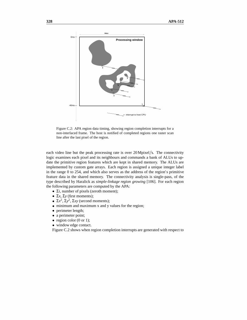
328 APA-512
1
2
3
4
5
6
7
= interrupt to host CPU
64us
Processing window
40ms
0ms
FigureC.2: APA region datatiming, showing region completioninterruptsfor anon-interlacedframe. The host is notifiedof completedregionsonerasterscanline afterthelastpixel of theregion.
eachvideo line but the peakprocessingrateis over 20Mpixel s. The connectivitylogic examineseachpixel andits neighboursandcommandsa bankof ALUs to up-datethe primitive region featureswhich arekept in sharedmemory. The ALUs areimplementedby customgatearrays. Eachregion is assigneda uniqueinteger labelin the range0 to 254,andwhich alsoservesasthe addressof the region's primitivefeaturedatain the sharedmemory. The connectivity analysisis single-pass,of thetypedescribedby Haralickassimple-linkageregion growing [106]. For eachregionthefollowing parametersarecomputedby theAPA:
Σi, numberof pixels(zerothmoment);Σx, Σy (first moments);Σx2, Σy2, Σxy (secondmoments);minimumandmaximumx andy valuesfor theregion;perimeterlength;a perimeterpoint;region color (0 or 1);window edgecontact.
FigureC.2showswhenregioncompletioninterruptsaregeneratedwith respectto

APA-512 329
theimagewhichis input in rasterscanfashion.Oneline timeafterthelastpixel of theregion its completioncanbedetectedandthe hostcomputernotifiedby interruptorpollablestatusflag andthatregion's labelis placedin a queue.Thehostwouldreadalabelfrom thequeueandthenreadtheregion'sprimitivefeaturedatafrom theAPA'ssharedmemory. Informationaboutregionsis thusavailablewell beforetheendof thefield or framecontainingtheregion.
From the fundamentalparameters,a numberof commonlyusedimagefeaturesdiscussedin Section4.1suchas:
areacentroidlocationcircularitymajorandminor equivalentellipseaxislengthsobjectorientation(anglebetweenmajoraxisandhorizontal)
may becomputedby the hostprocessor. Theserepresenta substantialsubsetof theso-called'SRI parameters'definedby GleasonandAgin atSRI in thelate70's.
Theperimeterpoint is thecoordinateof onepixel on theregion'sperimeter, andisusedfor thosesubsequentoperationsthatrequiretraversalof theperimeter. Theedgecontactflag, whenset, indicatesthat the region touchesthe edgeof the processingwindow andmaybepartially out of theimage,in this casetheparameterswouldnotrepresentthecompleteobject.
Perimeteris computedby a schemethat examinesa 3x3 window aroundeachperimeterpoint asshown in FigureC.3. The lookup tableproducesan appropriateperimeterlengthcontributiondependingupontheslopeof theperimeterat thatpoint.Experimentsrevealaworstcaseperimetererrorof 2%with thisscheme.
The APA-512 computestheseparametersfor eachof up to 255 current regionswithin thescene.Processingof thedatais donein rasterscanfashion,andastheendof a region is detectedtheregion label is placedin a queueandthehostis notifiedbyaninterruptor apollablestatusflag. Thehostmayreadtheregionparametersandthenreturntheregionlabelto theAPA for reuselaterin theframe,thusallowingprocessingof morethan255 objectswithin oneframe. This featureis essentialfor processingnon-trivial sceneswhichcancontainseveralhundredregionsof whichonly a few areof interest.Maximumprocessingtime is onevideoframetime.
An additionalfeatureof theAPA is its ability to returnregion hierarchyinforma-tion asshown in FigureC.4. Whena region is completethe APA may bepolled torecover the labelsof alreadycompletedregionswhich weretopologicallycontainedwithin that region. This makesit possibleto count the numberof holeswithin anobject,andcomputetheareaof enclosedholesor internalperimeter.
The APA wasdesignedto processnon-interlacedvideo,but canbe coercedintoworking with interlacedvideo thuseliminatingthe deinterlacingprocess.The APAprocessesthe interlacedvideo as one large frame,seeFigureC.5. The active pro-cessingwindow is set to the upperpositionbeforethe even field commences.This

330 APA-512
0 0 1 1 1 1 1 1 1LOOK UP TABLE
PERIMETER SUM ALU
FigureC.3: Perimetercontribution lookupscheme.
window stopsprocessingbeforetheblankingintervalduringwhichtime theAPA willcontinueloadingthevideosignalwhich will comprisetheequalizationandserrationpulses.Prior to theoddfield commencing,theprocessingwindow is setto thelowerposition.Thebiggestdrawbackwith this approachis thatthebottomprocessingwin-dow comprisesonly 511 313 198linesratherthanthe287active linesof a videofield. This is dueto the APA unnecessarilyloadinglines during the vertical blank-ing interval andalsotheCCIR videoformathaving 574active lines. Normally whenworkingwith 512 512imagesthelower31 linesof eachfield arelost.
TheAPA-512 is controlledby thehostcomputerusinga 'C' languagelibrary thatis compatiblewith Datacube's MAXWARE 3.1 [74]. To achieve maximumperfor-mancewith a Sun workstationhosta Unix device driver was written to efficientlymove datafrom the APA to theapplicationprogram's memoryspace.For operationunderVxWorkstheinterfacelibrary wassimply cross-compiledandthedevicedriverreplacedby a simplestructurein which APA interrupthandlersraisesemaphorestounblocktaskswhichservicetheAPA.

APA-512 331
1
2
4
5
6
7
3
1
2 3
47
5 6
Region hierarchy 3
FigureC.4: Hierarchyof binaryregions.
Odd fieldEven field
blanking interval287313
511
0
FigureC.5: Fieldmodeoperation.Stippledregionshowstheprogressof therasterscan.Dashedbox is theactiveAPA processingwindow.

332 APA-512

Appendix D
RTVL: a softwaresystemforrobot visual servoing
Thisappendixdiscussesasoftwaresystemdevelopedwithin theDivision'sMelbourneLaboratoryto facilitateresearchinto video-rateroboticvisualservoing. Early experi-mentalwork in visualservoing showedthatquitesimpleapplicationsrapidly becamebloatedwith detailedcodedealingwith the requirementsof vision and robot con-trol, graphicaldisplay, diagnostics,dataloggingandso on [57]. Considerableworkhasgoneinto thedesignof thesoftwaresystemknown asRTVL for real-timevisionlibrary. RTVL providesextensive functionsto theuser's applicationprogramencom-passingvisual-featureextraction,data-logging,remotevariablesetting,andgraphicaldisplay.
RTVL providesvisual-servo specificextensionsto VxWorks and is loadedintomemoryat systemboottime to providesall theinfrastructurerequiredfor visualser-voing. Visualservo applicationsprogramsareloadedsubsequentlyandaccessRTVLvia a well-definedfunctioncall interface.Internallyit comprisesa numberof concur-renttasksandshareddatastructures.EachRTVL modulehasits owninitializationandcleanupprocedureaswell asoneor moreprocedures,accessiblefrom theVxWorksshell, to show operatingstatisticsor enabledebuggingoutput. The wholesystemishighly parameterizedandtheparametersareparsedfrom a text file at startup.All pa-rametersareglobalvariables,andthusmaybeinspectedor alteredfrom theVxWorksshell allowing many operatingcharacteristicsto bechangedonline. A schematicofthesystem,showing bothhardwareandsoftwarecomponents,is givenin FigureD.1.
333

334 RTVL: a software systemfor robot visual servoing
digitizer
RGBmonitor
framebuffer
Application
Feature module Robotmodule
MATLAB datafile
binarizeandmedianfilter
Tracebuffer
performance metrics
variable watch
status
graphicsrenderingtask graphic
requestpipeline
camera
Utility
Kernel
Application
Parameterregistery
RPCserver
APA−512
hardware
FigureD.1: Schematicof theexperimentalsystem
D.1 Imageprocessingcontrol
The imageprocessingpipelineshown in Figure D.1 requiressoftwareinterventionduringeachvideoblankingtimeto controlvideodatapathsandsettheAPA processingwindow to allow field rateprocessingasdiscussedin AppendixC. Thefield taskisactivatedatthestartof videoblankingandinvokesfunctionsthathavebeenpreviouslyregisteredfor callback. A numberof permanentcallbacksareusedby RTVL itselfand othersmay be registeredby userapplicationprograms. The blanking intervalis relatively narrow, lastingonly 1.6ms,so this taskrunsat high priority in ordertoaccomplishall its taskswithin theblankinginterval. Datacube'sMAXWAREsoftwarelibrariesareused,with a customwritten low level moduleto allow operationunderVxWorks.
D.2 Imagefeatures
Thefeatureextractionprocessis simplisticandreportsthefirst (in rasterorder)n re-gionswhichmeettheapplicationprogram'sacceptancecriteria. Theseareexpressedin termsof a booleanscreeningfunctionappliedto all extractedregionsin thescene.Typically screeningis on thebasisof objectcolor (blackor white), upperandlower

D.3 Time stampsand synchronizedinterrupts 335
32 32
VMEbus
32−bit presettabledowncounter
overflow
VMEbusinterrupt
32
32
latch‘linetime’counter
MAXbus Hsync (15kHz)
MAXbus pixel clock (10MHz)
divisor
FigureD.2: Block diagramof video-lockedtiming hardware.
boundsonarea,andperhapscircularity(4.11).Functionsexist tocomputeusefulmea-suressuchascentroid,circularityandcentralmomentsfrom thereturnedregiondatas-tructures.An applicationobtainsregion datastructuresby meansof the regGet()function.
D.3 Time stampsand synchronizedinterrupts
Timestampingeventsis essentialin understandingthe temporalbehavior of a com-plex multi-taskingsensor-basedsystem.It is alsodesirablethat the mechanismhaslow overheadsoasnot to impacton systemperformance.To meetthis needa noveltiming boardhasbeendevelopedthat provides, via one 32-bit register, a count ofvideo linessincemidnight,seeFigureD.2. Eachvideo line lasts64µs andthis pro-videsadequatetiming resolution,but moreimportantlysincethecountis derivedfrom

336 RTVL: a software systemfor robot visual servoing
Task
Task
pipe
graphicsrendertask
Framestore512 x 512
camera
monitor
SunView pixrectlibraries
FigureD.3: Graphicsrenderingsubsystem.
MAXBUS horizontalsynchronizationsignalsit givesa time valuewhich canbedi-rectly relatedto the video waveform. The time valuecanbe readily convertedintoframenumber, field number, field type(oddor even)andline numberwithin thefieldor frame, as well as into conventionalunits suchas time of day in hours,minutesandseconds.A comprehensive groupof macrosandfunctionsis providedto performtheseconversions.For debuggingandperformanceanalysisthis allows thetiming ofeventswith respectto thevideowaveformto bepreciselydetermined.
In addition, for custommanipulatoraxis control strategies,a sourceof periodicinterruptswith a periodin therange1 to 5msis required.To avoid beatingproblemswith the lower ratevisualcontrol loopsit is desirablethat theservo loopsoperateata sub-multipleof thevision field time. A programmabledown counteron thetimingboarddividestheMAXBUS pixel clockbya32bit divisortocreatesuitableinterrupts.Divisorvaluesarecomputedby
n 9625000 T
whereT is thedesiredperiodin unitsof seconds.The2 and4msperiodservo loopsusedin Chapter8 areclockedin thismanner.

D.4 Real-timegraphics 337
Task
pipe
graphicsrendertask
camera
monitor
watchTask
"X=%82.f"&xc"Y=%8.2f"&yc
X=12.34Y=45.67
5Hz
FigureD.4: Variablewatchfacility.
D.4 Real-timegraphics
The systemusesa framebuffer to hold graphicaldatawhich is overlaid on the liveimagefrom thecamera.Almostall informationaboutthesystemcanbelearnedfromthis display. Sincemany tasksneedto display graphicalinformation quickly andcannotafford to wait all requestsarequeued,seeFigureD.3. Thegraphicalrequestsqueueis servicedby a low-priority taskwhich rendersthegraphicalentitiesinto theframebuffer usingtheSunView pixrectlibrarieswhichhasbeen'fooled' into treatingthe ROISTORE asa memoryresidentpixrect. Functionsareprovided which allowanapplicationto write stringsto thegraphicdisplayandupdatea varietyof trackingcursors.
D.5 Variable watch
The'watch' packageallowsanumberof specifiedvariablesto bemonitoredandtheirvaluedisplayedonthereal-timegraphicsdisplayasshown in FigureD.4. Thevariablevaluesareupdatedon thescreenat 5Hz, andmaybeusedto monitorvariousinternalprogramvariables,asshown in Figure6.8.

338 RTVL: a software systemfor robot visual servoing
D.6 Parameters
Most partsof the RTVL kernelarecontrolledby parameters,ratherthancompiled-in constants.Parameterscanbe integer, float or string variables,or beattachedto afunctionwhich is invokedwhentheparameteris changed.Whilst parameterscanbesetmanuallyvia the VxWorks shell, the preferredmechanismis via the interactivecontrol facility describednext. Parametersareinitialized from a parameterfile readwhenthekernelstartsup. As eachparameteris initializedfrom thefile, it is registeredwith theparametermanager, whichis aremoteprocedurecall (RPC)server taskwhichcanmodify or returnthe valueof any parameter, seeFigureD.5. Userapplicationscanalsousetheparameterfacilities,by explicitly registeringthetypeandlocationofapplicationprogramparameters.
D.7 Interacti vecontrol facility
Variousoperatingparametersof theRTVL kernelsuchasthresholdmaybechangedby simply moving a slideron thecontrolpanel.A popupwindow lists all parametersregisteredunderRTVL, anddouble-clickingbringsup a slider, or valueentry box,for thatparameter. TheXView programis anRPCclient to theparameterserver taskrunningunderVxWorksto examineandmodify theparameter.
Convenientcontrolof applicationsis facilitatedby a mechanismthatallows pro-gramvariablesto beregisteredwith a remoteprocedurecall (RPC)server. Theclientis aninteractivecontroltool runningunderOpenWindowsonanattachedworkstationcomputer. A list of variablesregisteredunderthereal-timesystemcanbepoppedup,andfor userselectedvariablesa valueslider is createdwhich allows thatvariabletobeadjusted.Variablescanbeboolean,integer, floatingpoint scalaror vector.
The namedparameterscanbeconvenientlyexaminedandmodifiedby the inter-active controltool, anXView applicationrunningunderOpenWindows.
A remotecursor facility hasalso beenimplemented,wherebya cursoron theRTVL displayis slaved to the mouseon the OpenWindows workstation. An appli-cationprogramcanwait for a 'pick' event
superGetPick(&coord);
Unsolicitedpicksaregrabbedby theregion processingsubsystemwhichwill displaythefeaturevectorfor theregion underthecursor.
D.8 Data loggingand debugging
The VxWorksshell allows any global programvariableto beexaminedor modifiedinteractively. Howeverit hasbeenfoundconvenienttobuild facilitiesto 'log' variables

D.8 Data loggingand debugging 339
parameterregistry
RPCserver
"Pgain" DOUBLE"Enable" BOOL"Thresh" INT
double Pgain;
paramRegister("Pgain", PARAM_TYPE, PARAM_REAL, PARAM_ADDR, &Pgain, NULL);
FigureD.5: On-lineparametermanipulation.
of interestonto themaincolor display, andalsoto recordtime historiesof variablesfor dataloggingpurposes.
The 'watch' facility continuouslydisplaysthe valuesof a nominatedlist of vari-ablesin thegraphicsplanewhichissuperimposedonthelivecameraimage,seeFigure6.8.
The RTVL kernelprovidesbuilt-in facilities to log multiple variablesduring anexperiment.This is essentialin trying to debug anapplication,or monitortheclosed-loop controlsystemperformance.Tracedvariablesaretimestampedandplacedinto

340 RTVL: a software systemfor robot visual servoing
a large circular buffer usinga low-overheadmacropackage. The tracebuffer canbedumpedto disk, andoff-line toolscanbeusedto extract the time historiesof thevariablesof interest.Thesetimerecordscanbeanalyzedby anumberof toolssuchasMATLAB [181] for analysisandplotting.
D.9 Robot control
Robotcontrolfunctionsarelayeredontopof theARCL packageintroducedin Section6.2.3.RTVL canuseARCL facilities to implementa 6-DOFCartesianvelocity con-troller. This approachis usefulfor quick applicationdevelopment,but theproblemsdiscussedin thebodyof thebooksuchasincreasedlatency from datadoublehandlingandthelimitationsof purelyfeedbackcontrolwill apply. For higherperformanceit isnecessaryfor theprogrammerto implementcustomaxiscontrolloops.
D.10 Application program facilities
MATLAB is usedasa tool for bothcontrollerdesignanddataanalysis.The RTVLkernel includeslibrary routinesfor readingMATLAB' s binary MAT-files, as wellasfor performingmatrix arithmetic. This allows straightforwardimplementationofstate-feedbackcontrollersandstate-estimatorsdesignedusingMATLAB. On thecur-rentsystem,a 4-stateestimatorandstate-feedbackcontrolcanbeexecutedin around500µs.
D.11 An example— planar positioning
Servoing in a planeorthogonalto thecameraview axishasbeendemonstratedby anumberof authorswith varyinglevelsof performance.Themostappropriatefeaturesto usearetheobjectcentroid xc yc , computedsimply from the1stordermoments;
xcm10
m00yc
m01
m00
Theessenceof theapplicationprogramis:
1 planar()2 3 Region r;4 double xc, yc, xgain, ygain, cartRates[6];5 int nfeat;67 paramRegister("xgain", &xgain, PARAM_TYPE, PARAM_REAL, 0);8 paramRegister("ygain", &ygain, PARAM_TYPE, PARAM_REAL, 0);

D.12Conclusion 341
9 watchStart("X=%f", &x, "Y=%f", &y, NULL);10 regFilterFunc(filterfn); /* specify region screening funcn */11 robotOpen();12 for (;;) /* loop forever */13 nfeat = regGet(&r, 1, filterfn); /* get a feature */1415 xc = XC(r); /* find the centroid */16 yc = YC(r);1718 /* compute the desired cartesian velocity */19 cartRates[X] = xc * xgain;20 cartRates[Y] = yc * ygain;2122 /* set the robot velocity */23 robotSetRates(cartRates);24 24
Lines7-8 registerthetwo controlgainswith theparametermanagerto allow set-ting by theremoteinteractive control tool. Line 9 causesthecentroidcoordinatesinpixelsto bemonitoredon thereal-timedisplay. Line 12 requestsa singlefeaturethatis acceptedby thelow-level region screeningfunction filterfn (not shown here).Next the centroid is computedfrom simple momentfeatureswithin the Regiondatatype,the control gain is computed,and then the X and Y Cartesianvelocitiesof therobotareset.
D.12 Conclusion
A powerful experimentalfacility for researchinto roboticvisual closed-loopcontrolhasbeendescribed.Pipelinedimageprocessinghardwareanda high-speedregion-analysisboardsetareusedto extractvisual featuresat 50Hz. TheRTVL kerneltakesadvantageof thereal-timemulti-taskingenvironmentto providefacilitiesfor real-timegraphics,statusdisplay, diagnostictracing,interactivecontrolvia aremoteOpenWin-dows control tool, andMATLAB dataimport. An importantdesignaim wasto de-couplethe actualapplicationfrom the considerableinfrastructurefor visual-featureextractionandrobotcontrol.

342 RTVL: a software systemfor robot visual servoing

Appendix E
LED strobe
FigureE.1: Photographof cameramountedsolid-statestrobe.
343

344 LED strobe
Activevideo
Video field time (20ms)
Time
Video blankingtime (1.6ms)
t2
t1
LED
delay
FigureE.2: Derivationof LED timing from verticalsynchronizationpulses.
Thehigh-powerLED illuminationsystembuilt in thecourseof this work is shown inFigureE.1. TenLEDs arearrangedin a circlearoundthelensproviding coaxialillu-minationof therobot'sareaof interest.FigureE.2showshow theLED timing pulsesarederived from vertical synchronizationpulsesoutputby the system's DIGIMAXvideodigitizer. Thefirst delay, t1, positionsthepulsewith respectto theverticalsyn-chronizationpulseandis usedto align theLED pulsewith theshutteropening.Theseconddelay, t2, governsthelengthof theLED pulse.LED timing canbereadilysetby pointing thecameraat theLED while observingthe cameraoutputon a monitor.TheLED appearslit only whentheLED pulseoverlapsthecameraexposureinterval.For a shortdurationpulse,theboundsof theexposureinterval canbeexplored.Suchanapproachwasusedto determinetheexposureintervalsshown in Figure3.14.
The peakpulsecurrentwasestablishedexperimentallyusinga circuit which al-lowed the currentwaveform to be monitoredwhile adjustingthe magnitudeof theappliedvoltagepulse.As thepeakcurrentamplitudeis increasedtheobservedcurrentwaveformceasesto besquareandrisesduringthepulse.This is indicativeof theonsetof thermalbreakdown within the junction,andif sustainedwasfoundto leadto per-manentdestructionof the LED. The relationshipbetweenpermissiblecurrentpulseamplitudeandduty cycle is likely to benonlinearanddependentuponthermalprop-ertiesof theLED junctionandencapsulation.Thefinal LED controlunit providesanadjustableconstantcurrentdrive to avoid destructive currentincreasedueto thermalbreakdown.
In practiceit wasfoundthat therelationshipbetweencurrentandbrightnesswasnon-linearasshown in FigureE.5.Furtherinvestigationwith ahigh-speedphotodiodesensor, seeFigureE.3,showsthatthelight outputof theLED is anarrow initial spikewith a slower exponentialfalloff. FigureE.4 shows moredetail of the initial spike.Thelight outputincreaseswith currentwhichhasalimited risetimedueto inductance

LED strobe 345
0.5 1 1.5 2 2.5 30
0.1
0.2
0.3
0.4
Time (ms)
Ligh
t (no
rmal
ized
)
0.5 1 1.5 2 2.5 30
0.1
0.2
0.3
Time (ms)
Cur
rent
(m
A)
FigureE.3: LED light outputasa functionof time. Notetheverynarrow initial peak.
0 10 20 30 40 500
0.1
0.2
0.3
0.4
0.5
Time (us)
Ligh
t (no
rmal
ized
)
0 10 20 30 40 500
0.1
0.2
0.3
Time (us)
Cur
rent
(m
A)
FigureE.4: LED light outputduring initial peak.Current(andlight output)risetime is limited by circuit inductance.

346 LED strobe
0 0.05 0.1 0.15 0.2 0.25 0.30
0.5
1
1.5
2
2.5
3
Current (mA)
Ligh
t out
put
FigureE.5: MeasuredLED intensity as a function of current. Intensity is theaverageintensityover many light pulsesas measuredwith an averaginglight-meter.
in thelong connectingcable.After thepeak,light outputfalls off exponentiallywitha time constantof approximately10µs. The two time constantsinvolved in lightfalloff aresuspectedto be dueto heatingeffects: the fast modefrom heatingof thesmall junction region, andthe slow modefrom heatingthe entirepackage.At hightemperatureanLED hasa reducedquantumefficiency andits spectralcharacteristicsmayalter[279].
This light sourcehasbeenusedusefully in many experiments.Themostsignif-icant difficulties arethat the light outputwas not asgreatashopedfor, due to theunexpectedthermaleffectsdescribedabove, andtheratherunevennatureof theillu-mination.

Index
α β filter, 245–246,248,249,252α β γ filter, 173,246f -number, 80
aberrationsin lens,84–85accuracy of robot,11AGC,seeautomaticgaincontrolaliasing
spatial,91,136temporal,115–116,269
ALTERfacility, VAL II, 174amplifier voltagesaturation,48, 234,
266analogservo board,seeUNIMATEPuma,
analogservo boardangleof view, 80APA-512+,180–181,327–330aperture,80ARCL robotcontrolsoftware,178–179arminterfaceboard,seeUNIMATEPuma,
arminterfaceboardarm-interfaceboard,177automaticgaincontrol,98–100axisvelocity control,233,234axisvelocity estimation,276
backEMF, 47,268blackbodyradiation,76
cameraactive video,109AGC,96,98–100angleof view, 80
calibration,107CCD,88–90
blooming,90crosstalk, 91,94exposurecontrol,94frametransfer, 90spectralresponse,76
CID, 90darkcurrent,100digital output,103dynamicrange,102electronicshutter, 120exposureinterval, 118eye-in-handconfiguration,3field shutter, 105frameshutter, 105gamma,96integrationperiod,94lag in centroid,94line scan,88,156metric,139modulationtransferfunction,91–
94MTF, 91–94,107,109NMOS,90noise,100–101,134nonmetric,139panandtilt, 184,185,236pixel cross-talk,90pixel dimensions,111principalpoint,138sensitivity, 96–100
347

348 INDEX
signalto noiseratio,101spatialsampling,91–94
cameracalibrationclassicalnon-linearmethod,141homogeneoustransformmethod,
141matrix,138techniques,139–145Tsai's method,143two planemethod,143
cameralocationdeterminationproblem,144
CCDinterlinetransfer, 89
CCDsensor, 166CCIRvideoformat,103centralprojection,87centripetaleffect,15centroid,127
accuracy of, 133accuracy of estimate,209biasdueto aliasing,136effect of threshold,133errorfor off-axisviewing, 127lag in estimate,94,206of disk,133useof, 284
chargewell, 88CIE luminosity, 75circleof confusion,83,118circularity, 128,206close-rangephotogrammetry, 138closed-loopbandwidth,211,214color temperature,76color, useof, 87,166communicationsto robotcontroller, 173compensatorstability, 220compliance
structural,194,233transmission,233,269–274
compoundlens,84
computed-torquecontrol,62,274–279,285–287
computervision,123connectivity analysis,328Coriolis effect,15,60,290Coulombfriction, seefrictionCRT monitor, luminanceresponse,95cyclotorsion,122
darkcurrent,100Datacube
DIGIMAX, 107–109,113,180MAXBUS, 180,184,327useof, 179–181
deinterlacing,105–106Denavit andHartenberg notation,8
modified,10depthof field, 83diffraction,136digitalservo board,seeUNIMATEPuma,
digital servo boarddigital velocity loop,239–242,252direct dynamics,seeforward dynam-
icsdynamiclookandmovevisualcontrol,
153dynamics,robot,seerigid-bodydynam-
ics
edgesharpness,134effect of noise,135electronicassembly, 264electronicshutter, 94,180,198endpointoscillation,268–269EV, seeexposurevalueexposure,82exposureinterval, 180,208exposurevalue,82extrinsic parameter, 138eye-handcalibration,147
feature

INDEX 349
extraction,127tracking,168vector, 153
feedforwardcontrol,214of rigid-bodydynamics,62visualservo, 235–236,251–257
film speed,82fixation,153,161,191,212,214,224,
236,251,253,255by orientation,188,192by translation,188humanreflex, 245,257
focal length,80,137focus,82–84,134
control,166depthof field, 83,118hyperfocaldistance,83,118
forwarddynamics,21fovea,153,257friction, 15,32–34,58,234,268,290
compensation,64,275–276Coulomb,32,46estimation,33static,32stiction,32viscous,32,46
gamma,96gearedtransmission,27geometricdistortion,85–86graspingmovingobject,155–157,173,
211gravity load,23
horizontalblanking,103humaneye
conephotorecptors,121fixationreflex, 257fovea,121,257muscles,121oculomotorsystem,257photopicresponse,74,76
rodphotoreceptor, 74saccadicmotion,121,257scotopicresponse,74smoothpursuit,121,257
hydraulicactuation,172hyperfocaldistance,83
illuminance,74,81illumination,118–121
fluorescent,77incandescent,76,118–120LED, 120–121,343–344theSun,74,76
imagefeature,123,153features,123–130,181,191Jacobian,162,165moments,127–130,167,180,328window basedprocessing,168–
169image-basedvisual servo, 153, 161–
165independentjoint control,60inertia,58,264–265
armature,22,28,37matrixof manipulator, 15normalized,264normalizedjoint, 28principalaxes,22productsof, 22
infra-redradiation,79insectvision,161integralaction,54,234,252interactionmatrix,164interlacedvideo,103–104,181intrinsicparameter, 138
Jacobiancameramount,185,285image,162,165,188manipulator, 10,185,285
350 INDEX
Kalmanfilter, 173,240,246–249,252,257
kinematicsforward,10inverse,10,192parametersfor Puma560,12–14singularity, 10
Lambertianreflection,75latency, 211
deinterlacing,181lens
aberration,84–85,114aperture,80,85C-mount,114compound,81,84,189diffraction,85,114,118equation,80,137focal length,80gain,188,189,197,206,269magnification,80modelling,188MTF, 85nodalpoint,189–191nodalpointestimation,190projectionfunction,86–87,152radialdistortion,86simple,79,189vignetting,84
light, 73light meter, 81–82
exposurevalue,82incidentlight, 81–82reflectedlight, 82spotreading,82,97
light stripe,156,159line scansensor, 88,156line spreadfunction,85lumens,73luminance,74,76luminosity, 73
luminousflux, 73luminousintensity, 74
machinevision,123magneto-motive force,38maneuver, 168, 173, 211, 245, 246,
249mechanicalpole,37medianfilter, 180metriccamera,139MMF, seemagneto-motive forcemodulationtransferfunction,85,113–
115moment
computation,167–168momentsof inertia,22motionblur, 115,166,204,253,266motionstereo,160,161,165motor
armatureandcurrentloopdynam-ics,45–47
armatureimpedance,41–42armatureinertia,22,28,37armaturereaction,38,40backEMF, 36,39contactpotentialdifference,36electricalpole,36magnetization,38,39MATLAB model,42,49mechanicalpole,35,51torqueconstant,33,35,38–41torquelimit, 46
MTF, seemodulationtransferfunctionmulti-ratesystem,194,196,201–203
nestedcontrolloops,228nodalpoint,189–191nonmetriccamera,139normalizedinertia,28
oculomotor, 257opticalaxis,79

INDEX 351
opticalflow, 167
parametersensitivity, 234perspective transformation,86–87photogrammetery
cameracalibrationmatrix,138cameralocationdetermination,144
photogrammetry, 137–147,159cameracalibration,139–145close-range,138poseestimation,159
photometricunits,75photometry, 73photonshotnoise,100photonsperlumen,78photopicresponse,74photosites,88pixel aspectratio,111–112pixel quantization,112pixel resampling,109,110pixel responsenon-uniformity, 101Planck'sequation,78poleplacement,221pose,3, 151–153poseestimation,153,159position-basedvisualservo, 153,159–
161prediction,173, 211, 219, 220, 245,
247principalaxesof inertia,22principalpoint,138productsof inertia,22
quantumefficiency, 96
radiantflux, 73radiometry, 73rasterscan,103RCCL,24,174,178recursive Newton-Euler, 286redundantmanipulator, 10reflectivity, 75
repeatabilityof robot,12resolvedratecontrol,285resolvedratemotioncontrol,11,192rigid-bodydynamics,14–19
baseparameters,23computationalissues,64–70controlof
computedtorque,62,63,274–279,285–287
feedforward,62,63equationsof motion,14forwarddynamics,21gravity load,23,33,34,58inertialparametersfor Puma560,
21–27inversedynamics,14recursive Newton-Euler, 16–19significanceof, 58–60,290symbolicmanipulation,19–21
robotaccuracy, 11dynamics,seerigid-bodydynam-
icsgeared,27joints,7kinematics,seekinematicslimitationsof, 1–2links, 7repeatability, 12
RS170videoformat,102RTVL software,182–184
saccadicmotion,257samplerate,234sampler
cameraas,198samplingrate,275scotopicresponse,74semi-anglesof view, 80serial-linkmanipulators,7signalto noiseratio,101,113,118

352 INDEX
SIMULINK modelCTORQUEJ1,275DIGVLOOP, 242FFVSERVO, 253LMOTOR, 50,234MOTOR,50POSLOOP, 57VLOOP, 52
Smith'smethod,218smoothpursuitmotioni,seefixationSNR,seesignalto noiseratiospecularreflection,75stadimetry, 284stateestimator, 220statefeedback,219steady-stateerror, 213steeringproblem,235stereovision,157,158,160,161,167
motionstereo,161,165stick/slipphenomena,234,276stiction,276structuraldynamics,194,201,263,268,
275symbolicmanipulation
recursive Newton-Euler, 19–21truncationof torqueexpression,67–
68
tachometer, 40,50targetcentroid,191targettracking,168teleoperation,169threshold
effect onaliasing,116effect oncentroidestimate,133effectonwidthestimate,131–133selection,135
thresholding,167,180timestamping,184,253,269trackingfilter
α β, 245–246
α β γ, 246comparisonof, 248–250initiation, 248,252Kalman,246–247lag in, 249–250,253maneuver, 168,173,211,245,246,
249roughnessof, 249–250trackingparameter, 246
trajectorygeneration,191,265–266Type,of system,213,231,234,257
UNIMATE Pumaamplifiervoltagesaturation,48analogservo board,50arminterfaceboard,179,240currentcontrolmode,56,239currentloop,42–44,228,270
currentlimit, 46digital servo board,52,179,237encoderresolution,53fundamentalperformancelimits,
56fuse,46gearratios,28kinematicparameters,12–14position loop, 52–55, 177, 266,
269,278controllaw, 54integralaction,54setpointinterpolation,53
velocity loop, 49–51, 229, 237,270,275,278
synthetictachometer, 50velocity limit, 237,267
wrist cross-coupling,27,40,252
velocity estimation,239,275of joint, 62quantization,239,276
velocity loop,digital, 239–242video

INDEX 353
amplitudeof signal,104,105backporch,104,107black-setupvoltage,104CCIR,103,110compositecolor, 104,107DC restoration,107digitization,106–113horizontalblanking,103interlaced,103–104pedestalvoltage,104rasterscanning,103RS170,102,110verticalblanking,104
viscousfriction, seefrictionvisualservo
advantageof, 2applications,154–159
catching,157fruit picking,157,172humanskills, 157vehicleguidance,157
asa steeringproblem,191axiscontrolmode
position,231torque,228velocity, 229
cameraassampler, 115,198closed-loopfrequency response,196,
206control
feedforward,214,235–236,251–257,284
LQG, 225PID, 216pole-placement,221Smith'smethod,218stabilityof compensator, 220statefeedback,219
controlproblem,191dynamics,151endpointdamping,279–281
imageJacobian,162,165kinematics,151latency in, 211neuralnetworksfor, 158performancemetric,214phaseresponse,214sampler, 253squarewave response,195stability problem,172taskspecification,169useof color, 166,167
VMEbus,176,180,327VxWorksoperatingsystem,177
width estimate,131effect of edgegradient,134
Wien's displacementlaw, 78
zerosof system,217,235