Vision-based target tracking with a small UAV: Optimization-basedcontrol strategies

Steven A.P. Quintero n,1, João P. Hespanha 1

Electrical and Computer Engineering, University of California, Santa Barbara, CA 93106, USA

a r t i c l e i n f o

Article history:Received 30 April 2013Accepted 19 July 2014

Keywords:Unmanned aerial vehicleTarget trackingMotion planningAutonomous vehicle

a b s t r a c t

This paper considers the problem of a small, fixed-wing UAV equipped with a gimbaled cameraautonomously tracking an unpredictable moving ground vehicle. Thus, the UAV must maintain closeproximity to the ground target and simultaneously keep the target in its camera's visibility region. Toachieve this objective robustly, two novel optimization-based control strategies are developed. The firstassumes an evasive target motion while the second assumes a stochastic target motion. The resultingoptimal control policies have been successfully flight tested, thereby demonstrating the efficacy of bothapproaches in a real-world implementation and highlighting the advantages of one approach overthe other.

& 2014 Elsevier Ltd. All rights reserved.

1. Introduction

The purpose of this work is to detail the design of two differentcontrol policies that enable a small, fixed-wing unmanned aerialvehicle (UAV), equipped with a pan-tilt gimbaled camera, to auto-nomously track a moving ground vehicle (target). The specificcontrol objective is best described by Saunders (2009) in Section4.1, where he defines vision-based target tracking as “maintaining atarget in the field-of-view of an onboard camera with sufficientresolution for visual detection.”

The class of UAV platforms under consideration are small,fixed-wing aircraft that are battery-powered and either hand orcatapult launched. Specific to the UAV used in the flights experi-ments is a mechanical limitation of the pan-tilt gimbal mechanismthat requires the UAV to keep the target towards its left-hand sidefor visibility. Nonetheless, by adjusting the cost function of thedynamic optimization, this work can be adapted to the fixed-camera scenario that is common on smaller platforms such asMicro Air Vehicles (MAVs). The sensor visibility constraint coupledwith uncertain target motion and underactuated UAV dynamicscompose the control challenge for which two novel solutions arepresented.

1.1. Contributions

Two different styles of optimization-based control policies aredeveloped to enable a small UAV to maintain visibility and proximityto target in spite of sensor blind spots, underactuated dynamics, andevasive or stochastic nonholonomic target motion. The first is agame theoretic approach that assumes evasive target motion. Hence,the problem is formulated as a two-player, zero-sum game withperfect state feedback and simultaneous play. The second is astochastic optimal control approach that assumes stochastic targetmotion. Accordingly, in this approach, the problem is treated in theframework of Markov Decision Processes (MDPs). In both problemformulations, the following are key features of the control design:

1. The UAV and the target are modeled by fourth-order discretetime dynamics, including simplified roll (bank) angle dynamicswith the desired roll angle as the control input.

2. The UAV minimizes an expected cumulative cost over a finitehorizon.

3. The cost function favors good viewing geometry, i.e., visibilityand proximity to the target, with modest pan-tilt gimbalangles.

4. The dynamic optimization is solved offline via dynamic pro-gramming.

Both approaches incorporate roll dynamics because the rolldynamics can be on the same time scale as the heading dynamics,even for small (hand-launched) UAVs. Accordingly, this work

Contents lists available at ScienceDirect

journal homepage: www.elsevier.com/locate/conengprac

Control Engineering Practice

http://dx.doi.org/10.1016/j.conengprac.2014.07.0070967-0661/& 2014 Elsevier Ltd. All rights reserved.

n Corresponding author.E-mail addresses: quintero@ece.ucsb.edu (S.A.P. Quintero),

hespanha@ece.ucsb.edu (J.P. Hespanha).1 Authors are with UCSB's Center for Control, Dynamical Systems, and

Computation.

Control Engineering Practice 32 (2014) 28–42

directly addresses the phase lag in the heading angle introducedby a comparatively slow roll rate that would otherwise be detri-mental to the UAV's tracking performance. Additionally, for smallaircraft, the range of permissible airspeeds may be very limited,as noted in Collins, Stankevitz, and Liese (2011), while frequentchanges in airspeed may be either undesirable for fuel economyor unattainable for underactuated aircraft. Thus, both controlapproaches assume a constant airspeed and treat the desired rollangle of the aircraft as the sole control input that affects thehorizontal plant dynamics. The target is modeled as a nonholo-nomic vehicle that turns and accelerates.

In order to determine control policies (decision rules for thedesired roll angle) that facilitate good viewing geometry, a costfunction is introduced to penalize extreme pan-tilt angles as wellas distance from the target. Dynamic programming is used tocompute (offline) the optimal control policies that minimize theexpected cumulative cost over a finite planning horizon. Thecontrol policies are effectively lookup tables for any given UAV/target configuration, and hence they are well suited for embeddedimplementations onboard small UAVs. These control policies havebeen successfully flight tested on hardware in the field, therebyverifying their robustness to unpredictable target motion, unmo-deled system dynamics, and environmental disturbances. Lastly,although steady wind is not directly addressed in the problemformulation, high fidelity simulations were performed that bothverify and quantify the policies' inherent robustness to light andeven moderate winds as well.

1.2. Related work

Significant attention has been given to the target trackingproblem in the past decade. Research groups have approached thisproblem from several different vantage points, and hence notablework from these perspectives is now highlighted. One line ofresearch proposes designing periodic reference flight trajectoriesthat enable the UAV to maintain close proximity to the target as ittracks the reference trajectories via waypoint navigation (Lee et al.,2003) or good helmsman steering (Husby, 2005). Although onereference trajectory is typically not suitable for all target speeds, onecan optimally switch between them based on UAV-to-target speedin order to minimize the maximum deviation from the target(Beard, 2007). A particularly unique line of work on target trackingis that of oscillatory control of a fixed-speed UAV. In this approach,one controls the amplitude and phase of a sinusoidal heading-rateinput to a kinematic unicycle such that the average velocity alongthe direction of motion equals that of the ground target, which isassumed to be piecewise constant (Lalish, Morgansen, & Tsukamaki,2007; Regina & Zanzi, 2011). None of the preceding works, however,consider any limitations imposed by miniature vision sensors thatare common on small, inexpensive UAVs.

Perhaps the greatest amount of research in the general areaof target tracking is devoted to solving the specific problem ofstandoff tracking. The control objective for this problem is to have aUAV orbit a moving target at a fixed, planar standoff distance. Frew(2007a) uses a Lyapunov guidance vector field (LGVF) approach toachieve the said objective. Summers (2010) builds upon the work ofFrew and further assumes that the target and wind speeds areunknown. Using the LGVF approach and adaptive estimates of thecombined wind and target velocity, Summers determines controllaws that provably achieve the desired standoff tracking objectivealong with a conservative upper bound on the maximum combinedwind/target speed that can be tolerated due to airspeed limitations.

Whereas the previous two lines of work did not considersensor limitations, there is a line of work, based on nonlinearfeedback control of the UAV's heading rate, wherein vision-sensorrequirements are addressed. Dobrokhodov, Kaminer, Jones, and

Ghabcheloo (2006) develop control laws for controlling botha UAV and its camera gimbal. The authors design nonlinear controllaws to align the gimbal pan angle with the target line-of-sight(LOS) vector and the UAV heading with the vector tangent tothe LOS vector; however, only uniform ultimate boundednessis proved. Li, Hovakimyan, Dobrokhodov, and Kaminer (2010)advance the previous work by reformulating the control objective,adapting the original guidance law, and proving asymptoticstability of the resultant closed-loop, non-autonomous system. Liet al. (2010) further adapt this newly designed control law toachieve asymptotic stability for the case of time-varying targetvelocity, although it comes at the high cost of requiring airspeedcontrol as well as data that is nontrivially acquired, namely thetarget's turn rate and acceleration. Saunders and Beard (2008)consider using a fixed-camera MAV to perform vision-based targettracking. By devising appropriate nonlinear feedback control laws,they are able to minimize the standoff distance to a constant-velocity target, while simultaneously respecting field of view(FOV) and max roll angle constraints.

Anderson and Milutinović (2011) present an innovative approachto the standoff tracking problem by solving the problem usingstochastic optimal control. Modeling the target as a Brownian particle(and the UAV as a deterministic Dubins vehicle), the authors employspecialized value iteration techniques to minimize the expected costof the total squared distance error discounted over an infinitehorizon. As no penalty is imposed on the control value, the resultingoptimal control policy is a bang-bang turn-rate controller that ishighly robust to unpredictable target motion. However, the discon-tinuous turn rate and absence of sensor limitations render thecontrol policy infeasible in a real-world implementation.

Others have also employed optimal control to address thegeneral target tracking problem, wherein the optimization criter-ion is mean-squared tracking error. Ponda, Kolacinski, and Frazzoli(2009) consider the problem of optimizing trajectories for a singleUAV equipped with a bearings-only sensor to estimate and trackboth fixed and moving targets. By performing a constrainedoptimization that minimizes the trace of the Cramer–Rao LowerBound at each discrete time step, they show that the UAV tends tospiral towards the target in order to increase the angular separa-tion between measurements while simultaneously reducing itsdistance to the target. While Ponda's approach is myopic, i.e., nolookahead, and controls are based on the true target position,Miller, Harris, and Chong (2009) propose a non-myopic solutionthat selects the control input based on the probability distributionof the target state, where the distribution is updated by a Kalmanfilter that assumes a nearly constant velocity target model.Moreover, Miller poses the target tracking problem as a partiallyobservable Markov decision process (POMDP) and presents a newapproximate solution, as nontrivial POMDP problems are intract-able to solve exactly (Thrun, Burgard, & Fox, 2005).

While the present paper focuses on target tracking with asingle UAV, there is also notable work devoted to coordinating twoor more UAVs to perform cooperative target geolocation (localiza-tion) and tracking. Such work generally aims at achieving coordi-nated standoff tracking, wherein two UAVs coordinate the phase oftheir fixed-radius orbits about the target in order to improvegeolocation estimates and/or obtain a diversity of viewing angles.For example, Oh, Kim, Tsourdos, and White (2013) propose atangent vector field guidance strategy for coordinated standofftracking with multiple UAVs wherein they employ sliding modecontrol with adaptive terms in order to mitigate the effects ofdisturbances and unmodelled dynamics. With estimates of thetarget state from a decentralized information filter, the UAVsachieve a desired angular separation in a decentralized fashionunder various information/communication architectures by chan-ging either airspeed or the nominal orbit radius. The problem has

S.A.P. Quintero, J.P. Hespanha / Control Engineering Practice 32 (2014) 28–42 29

been approached from alternative vantage points in Frew (2007b),Wheeler et al. (2006), and Kingston (2007). While such worktypically uses nonlinear feedback control, other have used optimalcontrol for the flight coordination of two UAVs. For example,Stachura, Carfang, and Frew (2009) develop an online recedinghorizon controller to maximize the total geolocation informationin the presence of communication packet losses, and Quintero,Papi, Klein, Chisci, and Hespanha (2010) determine optimal controlpolicies offline that minimize the joint geolocation error overa long planning horizon.

Although the present paper focuses on tracking a single targetwith one UAV, we note that tracking multiple ground targets withmultiple UAVs has received considerable attention as well. Oh,Kim, Shin, Tsourdos, and White (2013) use Frew's LGVF approachto achieve coordinated standoff tracking of clusters of targets usingmultiple UAV teams. Within each group, the nominal orbit radiusis set to ensure that each UAV maintains visibility of all targetsin the corresponding cluster, as each agent has a limited FOV.Furthermore, the UAV groups follow a set of rules to discard straytarget vehicles as well as ensure successful target handoff betweenteams. Miller et al. (2009) treat the problem of tracking multipletargets with multiple UAVs as a POMDP, wherein heuristics areemployed in the approximate solution to overcome the limitationsof short planning horizons in the presence of occlusions. Addi-tional work on the subject of multi-target tracking can be found inthe references of the aforementioned works.

None of the preceding works have considered a target thatperforms evasive maneuvers to escape the camera's FOV, yetsimilar problems have been addressed long ago in the contextof differential games (Isaacs, 1965). In particular, Dobbie (1966)characterized the surveillance-evasion game in which a variable-speed pursuer with limited turn radius strives to keep a constant-speed evader within a specified surveillance region. Lewin andBreakwell (1975) extend this work to a similar surveillance-evasion game wherein the evader strives to escape in minimumtime, if possible. While the ground target may not be evasive,treating the problem in this fashion will produce a UAV controlpolicy robust to unpre-dictable changes in target velocity.

In all of the preceding works, at least one or more assumptionsare made that impose practical limitations. Namely, the worksmentioned thus far assume at least one of the following:

1. Input dynamics are first order, which implies that roll dynamicshave been ignored.

2. Changing airspeed quickly/reliably is both acceptable and attai-nable.

3. Target travels at a constant velocity.4. Sensor is omnidirectional.5. Sinusoidal/orbital trajectories are optimal, including those

resulting from standoff tracking.

The work presented here removes all of these assumptions topromote a practical, robust solution that can be readily adapted toother similar target tracking applications that may have differentdynamics and hardware constraints. The policies also possess aninherent robustness that allow them to even track an unpredict-able target in the presence of light to moderate steady winds.

1.3. Paper outline

The remainder of the paper is organized as follows. Sections 2and 3 detail the game theoretic and stochastic optimal controlapproaches to vision-based target tracking, respectively. These sec-tions discuss the specific UAV and target dynamical models, thecommon cost function, and the individual dynamic programming

solutions. Section 4 describes the experimental hardware setup andalso presents the flight test results for each control approach.Furthermore, this section also provides a quantitative comparisonof the two approaches and draws conclusions concerning thepreferred control approach. Section 4 concludes by studying theeffects of wind on the performance of the policies in a high fidelitysimulation environment to quantify practical upper limits on thewind speeds that can be tolerated. Finally, Section 5 providesconclusions of the overall work and discusses venues for future work.

2. Game theoretic control design

This section details the game theoretic approach to vision-based target tracking. The key motivations for this approach are toremedy the usual constant-velocity target assumption seen inmuch of the literature and also to account for sensor visibilitylimitations. This is done by assuming that the target performsevasive maneuvers, i.e., it strives to enter the sensor blind spots ofthe UAV according to some control policy optimized to playagainst that of the UAV. Accordingly, the problem is posed as amulti-stage, two-player, zero-sum game with simultaneous playand solved with tools from noncooperative game theory. The twomain elements of a game are the actions available to the playersand their associated cost. Thus, the players' actions at each stageare first described, along with their respective dynamics. The costfunction of the viewing geometry is presented next and is thesame as that used in the stochastic approach. Lastly, this sectionpresents the formal problem statement and the dynamic program-ming solution that generates a control policy for each player.

2.1. Game dynamics

While the majority of work on target tracking uses continuoustime motion models, this work treats the optimization in discretetime. Thus, each player is initially modeled by fourth-ordercontinuous-time dynamics, and then a T-second zero-order hold(ZOH) is applied to both sets of dynamical equations to arrive atthe discrete-time dynamics of the overall system.

The UAV is assumed to have an autopilot that regulates pitch,airspeed, altitude, and commanded roll angle via internal feedbackloops, typically using Proportional-Integral-Derivative (PID) con-trol. Once every T seconds, the roll-angle setpoint is updatedaccording to the control policy for the game. The aircraft is furtherassumed to fly at a fixed airspeed and constant altitude above theground plane. Hence, the UAV's state comprises its planar positionðxa; yaÞAR2, heading ψ aAS1, and roll (bank) angle ϕAS1. Thus,the UAV state is defined as ξ≔ðxa; ya;ψ a;ϕÞ.

The UAV is modeled as a planar kinematic unicycle withsecond-order rotational dynamics, i.e.,

_ξ ¼ ddt

xayaψ a

ϕ

0BBBB@

1CCCCA¼

s cos ψ a

s sin ψ a

�ðαg=sÞ tan ϕ�αϕðϕ�rÞ

0BBBB@

1CCCCA; ð1Þ

where αg40 is the acceleration due to gravity and s denotes theairspeed, which is equivalent to the aircraft's groundspeed sincewe presently assume zero wind. Nonzero wind is addressed inSection 4.1. Furthermore, 1=αϕ40 is the time constant corre-sponding to the autopilot control loop that regulates the actual rollϕ to the roll-angle setpoint r. Most work in this area assumes thatαϕ is large enough so that there is a separation of time scalesbetween the heading dynamics _ψ a and the controlled rolldynamics _ϕ, and consequently, the roll dynamics can be ignored.However, when this assumption does not hold, the resultant phase

S.A.P. Quintero, J.P. Hespanha / Control Engineering Practice 32 (2014) 28–4230

lag introduced into the system can prove detrimental to targettracking performance. This is the case for small UAVs, like the oneused in the experimental work of the present paper, and hencesuch a simplifying assumption was avoided.

Applying a T-second ZOH to the UAV subsystem producesa discrete-time system ξþ ¼ f 1ðξ; rÞ that is obtained by solvingthe system of differential equations (1). The roll command r isassumed to belong to the set

C ¼ f0; 7Δ; 72Δg; ð2Þwhere Δ40 is the maximum allowable change in the roll setpointfrom one ZOH period to the next. Denoting the roll commandover the next ZOH period by r0, this work further stipulates thatr0AUðrÞ, where

UðrÞ≔fr; r7Δg \ C ð3Þis the roll-angle action space. This allows roll commands to changeby at most Δ and avoids sharp changes in roll that would bedetrimental to image processing algorithms in the target trackingtask (Collins et al., 2011).

The target is assumed to be a nonholonomic vehicle that travelsin the ground plane and has the ability to turn and accelerate. Itsstate comprises its planar position ðxg ; ygÞAR2, heading ψ gAS1,and speed vARZ0 and is hence defined as η≔ðxg ; yg ;ψ g ; vÞ. Thetarget's dynamics are those of a planar kinematic unicycle, i.e.,

_η ¼ ddt

xgygψ g

v

0BBB@

1CCCA¼

v cos ψ g

v sin ψ g

ωa

0BBB@

1CCCA; ð4Þ

where ω and a are the turn-rate and acceleration control inputs,respectively.

Applying a T-second ZOH to the target subsystem produces adiscrete-time system ηþ ¼ f 2ðη;dÞ that is obtained by solving (4)with d≔ðω; aÞ. To describe the target's action space, the set ofadmissible target speeds W is first introduced, along with thetarget's maximum speed v, which is assumed to be less than theUAV's airspeed. Denoting the target's maximum acceleration by a,the target's acceleration a is assumed to belong to the followingset:

DaðvÞ≔f0; ag; v¼ 0f�a;0; ag; vAW\f0; vgf�a;0g; v¼ v:

8><>: ð5Þ

Furthermore, with W ¼ f0; aT ;2aT ;…; vg, the set W is invariant inthe sense that vAW and aADaðvÞ implies vþ AW , as vþ ¼ aTþv.This property not only enforces speed bounds, but also improvesthe accuracy of the solution to the dynamic optimization. Denotingthe target's maximum turn rate by ω, the target's turn-rate ω isassumed to take on values in the following set:

DωðvÞ≔f0g; vAf0; vgf�ω;0;ωg; vAW\f0; vg:

(ð6Þ

This restriction on the turn rate implies that the target vehiclecannot turn while stopped nor while traveling at its maximumspeed v. Otherwise, it has the ability to turn left, go straight, orturn right using its maximum turn rate. The target's overall actionspace is defined as

DðvÞ≔DωðvÞ � DaðvÞ; ð7Þand hence dADðvÞ. Accordingly, depending on its current speed v,the target has anywhere from 2 to 9 action pairs from which tochoose at a given stage of the game.

The overall state of the game, ζAZ, is defined as

Z≔R2 � S1 � S1 � RZ0; ð8Þ

which combines the UAV and target states. The first 3 componentsof ζ are relative quantities in a target-centric coordinate frame,and the rest are absolute. The relative planar position in the target-centric coordinate frame is

ζ1ζ2

" #¼

cos ψ g sin ψ g

� sin ψ g cos ψ g

" #xa�xgya�yg

" #ð9Þ

while the remaining states are as follows:

ðζ3; ζ4;ζ5Þ ¼ ðψ a�ψ g ;ϕ; vÞ: ð10Þ

The overall dynamics of the game, ζ þ ¼ f ðζ ; r;dÞ, are givenimplicitly by f 1ðξ; rÞ and f 2ðη;dÞ and the preceding transforma-tions of the states in (9) and (10).

2.2. Cost objective

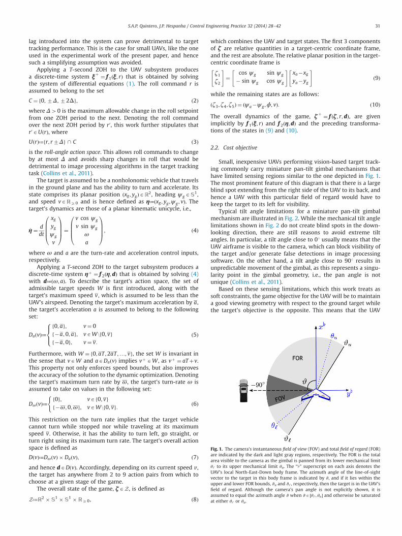
Small, inexpensive UAVs performing vision-based target track-ing commonly carry miniature pan-tilt gimbal mechanisms thathave limited sensing regions similar to the one depicted in Fig. 1.The most prominent feature of this diagram is that there is a largeblind spot extending from the right side of the UAV to its back, andhence a UAV with this particular field of regard would have tokeep the target to its left for visibility.

Typical tilt angle limitations for a miniature pan-tilt gimbalmechanism are illustrated in Fig. 2. While the mechanical tilt anglelimitations shown in Fig. 2 do not create blind spots in the down-looking direction, there are still reasons to avoid extreme tiltangles. In particular, a tilt angle close to 01 usually means that theUAV airframe is visible to the camera, which can block visibility ofthe target and/or generate false detections in image processingsoftware. On the other hand, a tilt angle close to 901 results inunpredictable movement of the gimbal, as this represents a singu-larity point in the gimbal geometry, i.e., the pan angle is notunique (Collins et al., 2011).

Based on these sensing limitations, which this work treats assoft constraints, the game objective for the UAV will be to maintaina good viewing geometry with respect to the ground target whilethe target's objective is the opposite. This means that the UAV

Fig. 1. The camera's instantaneous field of view (FOV) and total field of regard (FOR)are indicated by the dark and light gray regions, respectively. The FOR is the totalarea visible to the camera as the gimbal is panned from its lower mechanical limitθℓ to its upper mechanical limit θu. The “♭” superscript on each axis denotes theUAV's local North-East-Down body frame. The azimuth angle of the line-of-sightvector to the target in this body frame is indicated by ϑ, and if it lies within theupper and lower FOR bounds, ϑu and ϑℓ , respectively, then the target is in the UAV'sfield of regard. Although the camera's pan angle is not explicitly shown, it isassumed to equal the azimuth angle ϑ when ϑA ½θℓ ; θu� and otherwise be saturatedat either θℓ or θu.

S.A.P. Quintero, J.P. Hespanha / Control Engineering Practice 32 (2014) 28–42 31

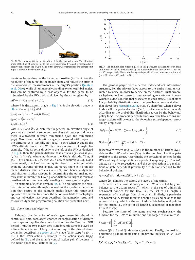
wants to be as close to the target as possible (to maximize theresolution of the target in the image plane and reduce the error inthe vision-based measurements of the target's position Quinteroet al., 2010), while simultaneously avoiding extreme gimbal angles.This can be captured by a cost objective for the game to beminimized by the UAV and maximized by the target given by

gðζÞ ¼ g1ðϑÞþg2ðφÞþg3ðρÞ; ð11Þwhere ϑ is the azimuth angle in Fig. 1, φ is the elevation angle inFig. 2, ρ¼

ffiffiffiffiffiffiffiffiffiffiffiffiffiffiffiζ21þζ22

q, and

g1ðϑÞ ¼ ðλ1 max fϑ�ϑ;0;ϑ�ϑgÞ2

g2ðφÞ ¼ λ22ðφ�π=4Þ2

g3ðρÞ ¼ ðλ3ρÞ2 ð12Þwith λi40 and ϑZϑ. Note that in general, an elevation angle ofφ¼ π=4 is achieved at some nonzero planar distance ρ, and hencethere is a tradeoff between minimizing g2ðφÞ and minimizingg3ðρÞ. Also, since the elevation angle is measured with respect tothe airframe, φ is typically not equal to π=4 when ρ equals theUAV's altitude, since the UAV often has a nonzero roll angle. Forexample, if the target is directly to the left of the UAV as depictedin Fig. 1, then the planar distance that achieves φ¼ π=4 is ρ¼ha= tan ðπ=4�ϕÞ, where ha denotes the UAV's altitude. Thus, ifϕ¼ �π=6 and ha¼170 m, then ρ¼ 45:55 m achieves φ¼ π=4, andconsequently the UAV can get quite close to the target whileavoiding extreme gimbal angles. Moreover, there is no uniqueplanar distance that achieves φ¼ π=4, and hence a dynamicoptimization is advantageous in determining the optimal trajec-tories that minimize the UAV's planar distance to target as much aspossible while simultaneously avoiding extreme gimbal angles.

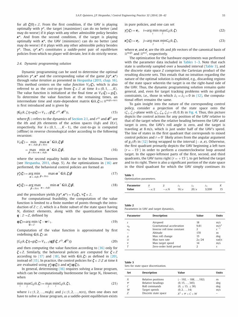
An example of g1ðϑÞ is given in Fig. 3. The plot depicts the zero-cost interval of azimuth angles as well as the quadratic penaliza-tion that occurs as the azimuth angles leave this range andapproach the extremities. Since the actions available to each playerand cost objective have been described, the gameplay setup andassociated dynamic programming solution are presented next.

2.3. Game setup and objective

Although the dynamics of each agent were introduced incontinuous-time, each agent chooses its control action at discretetime steps and applies the control action over the T-second ZOHperiod. Thus, the two-player, zero-sum dynamic game is played ona finite time interval of length K according to the discrete-timedynamics described in Section 2.1. At stage (time-step) kAf0;…;

K�1g, the UAV's action rk belongs to the action space UðϕkÞdefined in (3), and the target's control action pair dk belongs tothe action space DðvkÞ defined in (7).

The game is played with a perfect state-feedback informationstructure, i.e., the players have access to the entire state, uncor-rupted by noise, in order to decide on their actions. Furthermore,each player decides control actions according to a behavioral policy,which is a decision rule that associates to each state ζAZ at stagek a probability distribution over the possible actions available tothat player (see Hespanha, 2011, chap. 8). Therefore, when a playerfinds itself in a particular state ζAZ, it selects an action randomlyaccording to the probability distribution given by the behavioralpolicy for ζ . The probability distributions over the UAV actions andtarget actions will belong to the following state-dependent prob-ability simplexes:

AðϕÞ ¼ αARmðϕÞ : ∑iαi ¼ 1;αiZ0 8 i

( )ð13Þ

BðvÞ ¼ βARnðvÞ : ∑jβj ¼ 1;βjZ0 8 j

( ); ð14Þ

respectively, where mðϕÞ ¼ jUðϕÞj is the number of actions avail-able to the UAV and nðvÞ ¼ jDðvÞj is the number of action pairsavailable to the target. Accordingly, the behavioral policies for theUAV and target comprise time-dependent mappings γk : Z-AðϕÞand κk : Z-BðvÞ, respectively, and the control actions are realiza-tions of state-dependent probability distributions defined by thebehavioral policies:

rk � γkðζ ½k�Þ; dk � κkðζ ½k�Þ; 8kAf0;…;K�1g;where ζ ½k� denotes the state ζ at stage k of the game.

A particular behavioral policy of the UAV is denoted by γ andbelongs to the action space Γ1, which is the set of admissiblebehavioral policies for the UAV, i.e., the set of all length Ksequences of mappings from Z to AðϕÞ. Similarly, a particularbehavioral policy for the target is denoted by κ and belongs to theaction space Γ2, which is the set of admissible behavioral policiesfor the target, i.e., the set of all length K sequences of mappingsfrom Z to BðvÞ.

Because the state of the game evolves stochastically, thefunction for the UAV to minimize and the target to maximize is

Jðγ;κÞ ¼ E

"∑K

k ¼ 0gðζ ½k�Þjζ ½0�

#;

where ζ ½0�AZ and E½�� denotes expectation. Finally, the goal is todetermine a saddle-point pair of behavioral policies ðγn;κnÞ suchthat

Jðγn;κÞr Jðγn;κnÞr Jðγ;κnÞ; 8γAΓ1; 8κAΓ2

Fig. 2. The range of tilt angles is indicated by the shaded region. The elevationangle of the line-of-sight vector to the target is denoted by φ and is measured in apositive sense from the ðx♭ ; y♭Þ plane of the aircraft. For simplicity, the camera's tiltangle is taken to be the same as φ.

Fig. 3. The azimuth cost function g1ðϑÞ. In this particular instance, the pan anglelimitations, θℓ and θu, are indicated by the horizontal dashed lines at ϑ¼ �1351 andϑ¼ 151, respectively. The azimuth angle ϑ is penalized near these extremities withϑ¼ �901, ϑ ¼ �301, and λ1 ¼ 16π.

S.A.P. Quintero, J.P. Hespanha / Control Engineering Practice 32 (2014) 28–4232

for all ζ ½0�AZ. From the first condition, if the UAV is playingoptimally with γn, the target (maximizer) can do no better (andmay do worse) if it plays with any other admissible policy besidesκn. And from the second condition, if the target is playingoptimally with κn, the UAV (minimizer) can do no better (andmay do worse) if it plays with any other admissible policy besidesγn. Thus, ðγn;κnÞ constitutes a saddle-point pair of equilibriumpolicies fromwhich no player will deviate, lest it do strictly worse.

2.4. Dynamic programming solution

Dynamic programming can be used to determine the optimalpolicies γn;κn and the corresponding value of the game Jðγn;κnÞthrough value iteration as presented in Hespanha (2011, chap. 16).This method centers on the value function VkðζÞ, which is alsoreferred to as the cost-to-go from ζAZ at time kAf0;1;…;Kg.The value function is initialized at the final time as VK ðζÞ ¼ gðζÞ.To determine the value function at the remaining times, anintermediate time and state-dependent matrix Gðk; ζÞARmðϕÞ�nðvÞ

is first introduced and is given by

½Gijðk; ζÞ�≔gðζÞþVkþ1ðf ðζ ; rðiÞ;dðjÞÞÞ; ð15Þ

where f ð�Þ refers to the dynamics of Section 2.1, and rðiÞ and dðjÞ arethe ith and jth elements of the action spaces UðϕÞ and D(v),respectively. For kAf0;1;…;K�1g, the cost-to-go is computed(offline) in reverse chronological order according to the followingrecursion:

VkðζÞ ¼ minαAAðϕÞ

maxβABðvÞ

α>Gðk; ζÞβ

¼ maxβABðvÞ

minαAAðϕÞ

α>Gðk; ζÞβ; ð16Þ

where the second equality holds due to the Minimax Theorem(see Hespanha, 2011, chap. 5). As the optimizations in (16) areperformed, the behavioral control policies are formed as

γn

kðζÞ ¼ arg minαAAðϕÞ βABðvÞ

max α>Gðk; ζÞβ ð17Þ

κn

kðζÞ ¼ arg maxβABðvÞ αAAðϕÞ

min α>Gðk; ζÞβ; ð18Þ

and the procedure yields Jðγn;κnÞ ¼ V0ðζÞ; 8ζAZ.For computational feasibility, the computation of the value

function is limited to a finite number of points through the intro-duction of Z �Z, which is a finite subset of the state space havingNs distinct elements, along with the quantization functionq : Z-Z, defined by

qðζÞ≔arg minwAZ

Jζ�wJ1: ð19Þ

Computation of the value function is approximated by firstredefining Gðk; ζÞ as

½Gijðk; ζÞ�≔gðζÞþVkþ1ðq½f ðζ ; rðiÞ;dðjÞÞ�Þ ð20Þ

and then computing the value function according to (16) only forζAZ. Similarly, the behavioral policies are computed for ζAZaccording to (17) and (18), but with Gðk; ζÞ as defined in (20),instead of (15). In practice, the control policies for ζAZ\Z at time kare evaluated using γn

kðqðζÞÞ and κn

kðqðζÞÞ.In general, determining (16) requires solving a linear program,

which can be computationally burdensome for large Ns. However,when

mini

maxj

Gijðk; ζÞ ¼maxj

mini

Gijðk; ζÞ; ð21Þ

where iAf1;2;…;mðϕÞg and jAf1;2;…;nðvÞg, then one does nothave to solve a linear program, as a saddle-point equilibrium exists

in pure policies, and one can set

γn

kðζÞ ¼ ei; i≔arg mini

maxj

Gijðk; ζÞ ð22Þ

κn

kðζÞ ¼ ej; j≔arg maxj

mini

Gijðk; ζÞ; ð23Þ

where ei and ej are the ith and jth vectors of the canonical basis ofRmðϕÞ and RnðvÞ, respectively.

The optimization for the hardware experiments was performedwith the parameter data included in Tables 1–3. Note that eachstate is uniformly sampled over a bounded interval (Table 3), andthe discrete state space Z comprises the Cartesian product of theresulting discrete sets. This entails that no intuition regarding thenature of the optimal solution is exploited, e.g., discarding regionsof the state space wherein the target is on the right-hand side ofthe UAV. Thus, the dynamic programming solution remains quitegeneral, and, even for target tracking problems with no gimbalconstraints, i.e., those in which λ1 ¼ λ2 ¼ 0 in (12), the computa-tional effort remains the same.

To gain insight into the nature of the corresponding controlpolicy, consider a projection of the state space onto theðζ1; ζ2Þ-plane with ðζ3; ζ4; ζ5Þ ¼ ð0;0;8Þ in Fig. 4. Thus, this picturedepicts the control actions for any position of the UAV relative tothat of the target when the relative heading between the UAV andtarget is zero, the UAV's roll angle is zero, and the target istraveling at 8 m/s, which is just under half of the UAV's speed.The line of states in the first quadrant that corresponds to mixedcontrol policies and r¼ 01 likely arises from the angular argumentof g1ðϑÞ in (12) being wrapped to the interval ½�π;πÞ. Otherwise,the first quadrant primarily depicts the UAV beginning a left turn(r¼ �151) in order to perform a counterclockwise loop aroundtarget. In the upper-leftmost parts of the first, second, and thirdquadrants, the UAV turns right (r¼ þ151), to get behind the targetand to its right. There is also a significant portion of the state spacein the third quadrant for which the UAV simply continues its

Table 1Optimization parameters.

Parameter ϑ ϑ λ1 λ2 λ3 KValue �π=2 �π=6 16=π 20=π 3/200 15

Table 2Parameters in UAV and target dynamics.

Parameter Description Value Units

s Airspeed 18 m/sαg Gravitational acceleration 9.81 m/s2

αϕ Inverse roll time constant 2 s�1

– Altitude 170 mΔ Max roll change 15 degω Max turn rate 2π=24 rad/sv Max target speed 14 m/sT Zero-order hold period 2 s

Table 3Sets for state space discretization.

Set Description Value Units

X Relative positions f�192; �188;…;192g mΨ Relative headings f0;15;…;345g degC Roll commands f0; 715; 730g degW Target speeds f0;2;…;14g m/sZ Discrete state space X2 � Ψ � C �W –

S.A.P. Quintero, J.P. Hespanha / Control Engineering Practice 32 (2014) 28–42 33

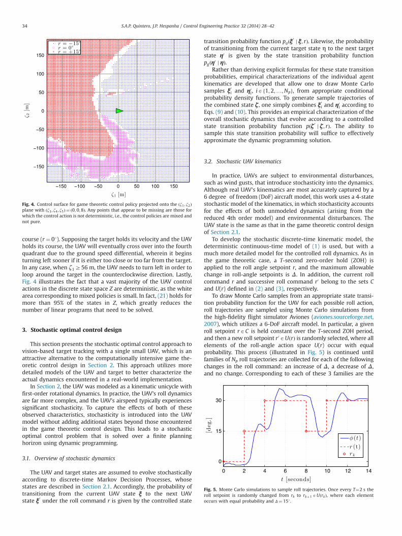
course (r¼ 01). Supposing the target holds its velocity and the UAVholds its course, the UAV will eventually cross over into the fourthquadrant due to the ground speed differential, wherein it beginsturning left sooner if it is either too close or too far from the target.In any case, when ζ1Z56 m, the UAV needs to turn left in order toloop around the target in the counterclockwise direction. Lastly,Fig. 4 illustrates the fact that a vast majority of the UAV controlactions in the discrete state space Z are deterministic, as the whitearea corresponding to mixed policies is small. In fact, (21) holds formore than 95% of the states in Z, which greatly reduces thenumber of linear programs that need to be solved.

3. Stochastic optimal control design

This section presents the stochastic optimal control approach tovision-based target tracking with a single small UAV, which is anattractive alternative to the computationally intensive game the-oretic control design in Section 2. This approach utilizes moredetailed models of the UAV and target to better characterize theactual dynamics encountered in a real-world implementation.

In Section 2, the UAV was modeled as a kinematic unicycle withfirst-order rotational dynamics. In practice, the UAV's roll dynamicsare far more complex, and the UAV's airspeed typically experiencessignificant stochasticity. To capture the effects of both of theseobserved characteristics, stochasticity is introduced into the UAVmodel without adding additional states beyond those encounteredin the game theoretic control design. This leads to a stochasticoptimal control problem that is solved over a finite planninghorizon using dynamic programming.

3.1. Overview of stochastic dynamics

The UAV and target states are assumed to evolve stochasticallyaccording to discrete-time Markov Decision Processes, whosestates are described in Section 2.1. Accordingly, the probability oftransitioning from the current UAV state ξ to the next UAVstate ξ0 under the roll command r is given by the controlled state

transition probability function paðξ0 j ξ; rÞ. Likewise, the probabilityof transitioning from the current target state η to the next targetstate η0 is given by the state transition probability functionpgðη0 j ηÞ.

Rather than deriving explicit formulas for these state transitionprobabilities, empirical characterizations of the individual agentkinematics are developed that allow one to draw Monte Carlosamples ξ0i and η0i, iAf1;2;…;Npg, from appropriate conditionalprobability density functions. To generate sample trajectories ofthe combined state ζ , one simply combines ξ0i and η0i according toEqs. (9) and (10). This provides an empirical characterization of theoverall stochastic dynamics that evolve according to a controlledstate transition probability function pðζ 0 j ζ ; rÞ. The ability tosample this state transition probability will suffice to effectivelyapproximate the dynamic programming solution.

3.2. Stochastic UAV kinematics

In practice, UAVs are subject to environmental disturbances,such as wind gusts, that introduce stochasticity into the dynamics.Although real UAV's kinematics are most accurately captured by a6 degree of freedom (DoF) aircraft model, this work uses a 4-statestochastic model of the kinematics, in which stochasticity accountsfor the effects of both unmodeled dynamics (arising from thereduced 4th order model) and environmental disturbances. TheUAV state is the same as that in the game theoretic control designof Section 2.1.

To develop the stochastic discrete-time kinematic model, thedeterministic continuous-time model of (1) is used, but with amuch more detailed model for the controlled roll dynamics. As inthe game theoretic case, a T-second zero-order hold (ZOH) isapplied to the roll angle setpoint r, and the maximum allowablechange in roll-angle setpoints is Δ. In addition, the current rollcommand r and successive roll command r0 belong to the sets Cand U(r) defined in (2) and (3), respectively.

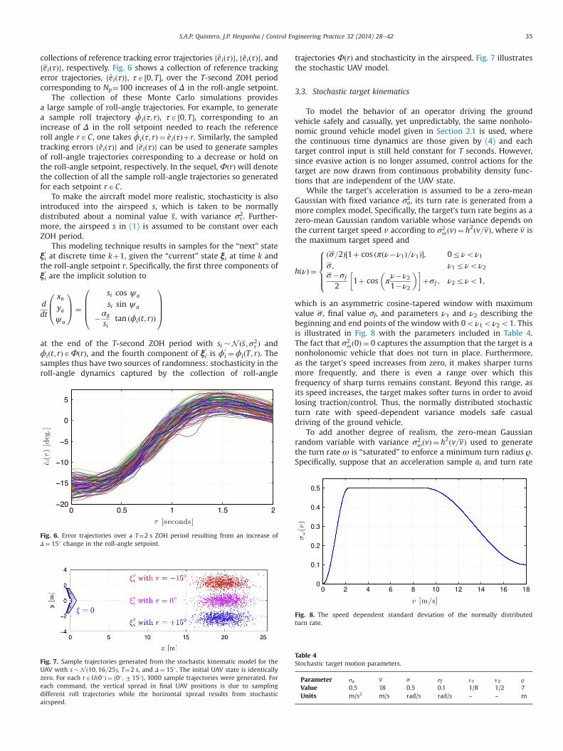
To draw Monte Carlo samples from an appropriate state transi-tion probability function for the UAV for each possible roll action,roll trajectories are sampled using Monte Carlo simulations fromthe high-fidelity flight simulator Aviones (aviones.sourceforge.net,2007), which utilizes a 6-DoF aircraft model. In particular, a givenroll setpoint rAC is held constant over the T-second ZOH period,and then a new roll setpoint r0AUðrÞ is randomly selected, where allelements of the roll-angle action space U(r) occur with equalprobability. This process (illustrated in Fig. 5) is continued untilfamilies of Np roll trajectories are collected for each of the followingchanges in the roll command: an increase of Δ, a decrease of Δ,and no change. Corresponding to each of these 3 families are the

Fig. 4. Control surface for game theoretic control policy projected onto the ðζ1 ; ζ2Þplane with ðζ3 ; ζ4 ; ζ5Þ ¼ ð0;0;8Þ. Any points that appear to be missing are those forwhich the control action is not deterministic, i.e., the control policies are mixed andnot pure.

Fig. 5. Monte Carlo simulations to sample roll trajectories. Once every T¼2 s theroll setpoint is randomly changed from rk to rkþ1AUðrkÞ, where each elementoccurs with equal probability and Δ¼ 151.

S.A.P. Quintero, J.P. Hespanha / Control Engineering Practice 32 (2014) 28–4234

collections of reference tracking error trajectories feiðτÞg, f �eiðτÞg, andfeiðτÞg, respectively. Fig. 6 shows a collection of reference trackingerror trajectories, feiðτÞg, τA ½0; T �, over the T-second ZOH periodcorresponding to Np¼100 increases of Δ in the roll-angle setpoint.

The collection of these Monte Carlo simulations providesa large sample of roll-angle trajectories. For example, to generatea sample roll trajectory ϕiðτ; rÞ, τA ½0; T �, corresponding to anincrease of Δ in the roll setpoint needed to reach the referenceroll angle rAC, one takes ϕ iðτ; rÞ ¼ eiðτÞþr. Similarly, the sampledtracking errors f �eiðτÞg and feiðτÞg can be used to generate samplesof roll-angle trajectories corresponding to a decrease or hold onthe roll-angle setpoint, respectively. In the sequel,ΦðrÞ will denotethe collection of all the sample roll-angle trajectories so generatedfor each setpoint rAC.

To make the aircraft model more realistic, stochasticity is alsointroduced into the airspeed s, which is taken to be normallydistributed about a nominal value s, with variance σs2. Further-more, the airspeed s in (1) is assumed to be constant over eachZOH period.

This modeling technique results in samples for the “next” stateξ0i at discrete time kþ1, given the “current” state ξi at time k andthe roll-angle setpoint r. Specifically, the first three components ofξ0i are the implicit solution to

ddt

xayaψ a

0B@

1CA¼

si cos ψ a

si sin ψ a

�αg

sitan ðϕiðt; rÞÞ

0BBB@

1CCCA

at the end of the T-second ZOH period with si �N ðs;σ2s Þ and

ϕiðt; rÞAΦðrÞ, and the fourth component of ξ0i is ϕ0i ¼ϕiðT ; rÞ. The

samples thus have two sources of randomness: stochasticity in theroll-angle dynamics captured by the collection of roll-angle

trajectories ΦðrÞ and stochasticity in the airspeed. Fig. 7 illustratesthe stochastic UAV model.

3.3. Stochastic target kinematics

To model the behavior of an operator driving the groundvehicle safely and casually, yet unpredictably, the same nonholo-nomic ground vehicle model given in Section 2.1 is used, wherethe continuous time dynamics are those given by (4) and eachtarget control input is still held constant for T seconds. However,since evasive action is no longer assumed, control actions for thetarget are now drawn from continuous probability density func-tions that are independent of the UAV state.

While the target's acceleration is assumed to be a zero-meanGaussian with fixed variance σa2, its turn rate is generated from amore complex model. Specifically, the target's turn rate begins as azero-mean Gaussian random variable whose variance depends onthe current target speed v according to σ2

ωðvÞ ¼ h2ðv=vÞ, where v isthe maximum target speed and

hðνÞ ¼

ðσ=2Þ½1þ cos ðπðν�ν1Þ=ν1Þ�; 0rνoν1σ ; ν1rνoν2σ�σf

21þ cos π

ν�ν21�ν2

� �� �þσf ; ν2rνo1;

8>>><>>>:

which is an asymmetric cosine-tapered window with maximumvalue σ , final value σf, and parameters ν1 and ν2 describing thebeginning and end points of the window with 0oν1oν2o1. Thisis illustrated in Fig. 8 with the parameters included in Table 4.The fact that σ2

ωð0Þ ¼ 0 captures the assumption that the target is anonholonomic vehicle that does not turn in place. Furthermore,as the target's speed increases from zero, it makes sharper turnsmore frequently, and there is even a range over which thisfrequency of sharp turns remains constant. Beyond this range, asits speed increases, the target makes softer turns in order to avoidlosing traction/control. Thus, the normally distributed stochasticturn rate with speed-dependent variance models safe casualdriving of the ground vehicle.

To add another degree of realism, the zero-mean Gaussianrandom variable with variance σ2

ωðvÞ ¼ h2ðv=vÞ used to generatethe turn rate ω is “saturated” to enforce a minimum turn radius ϱ.Specifically, suppose that an acceleration sample ai and turn rate

Fig. 6. Error trajectories over a T¼2 s ZOH period resulting from an increase ofΔ¼ 151 change in the roll-angle setpoint.

Fig. 7. Sample trajectories generated from the stochastic kinematic model for theUAV with s�N ð10;16=25Þ, T¼2 s, and Δ¼ 151. The initial UAV state is identicallyzero. For each rAUð01Þ ¼ f01; 7151g, 1000 sample trajectories were generated. Foreach command, the vertical spread in final UAV positions is due to samplingdifferent roll trajectories while the horizontal spread results from stochasticairspeed.

Fig. 8. The speed dependent standard deviation of the normally distributedturn rate.

Table 4Stochastic target motion parameters.

Parameter σa v σ σf ν1 ν2 ϱ

Value 0.5 18 0.5 0.1 1/8 1/2 7Units m/s2 m/s rad/s rad/s – – m

S.A.P. Quintero, J.P. Hespanha / Control Engineering Practice 32 (2014) 28–42 35

sample ~ωi are drawn from N ð0;σ2aÞ and N ð0;σ2

ωðvÞÞ, respectively.The turn rate ωi that is actually used is given by

ωi ¼ωi; ~ω i4ωi

~ωi; �ωir ~ω irωi

�ω i; ~ω io�ω i;

8><>:

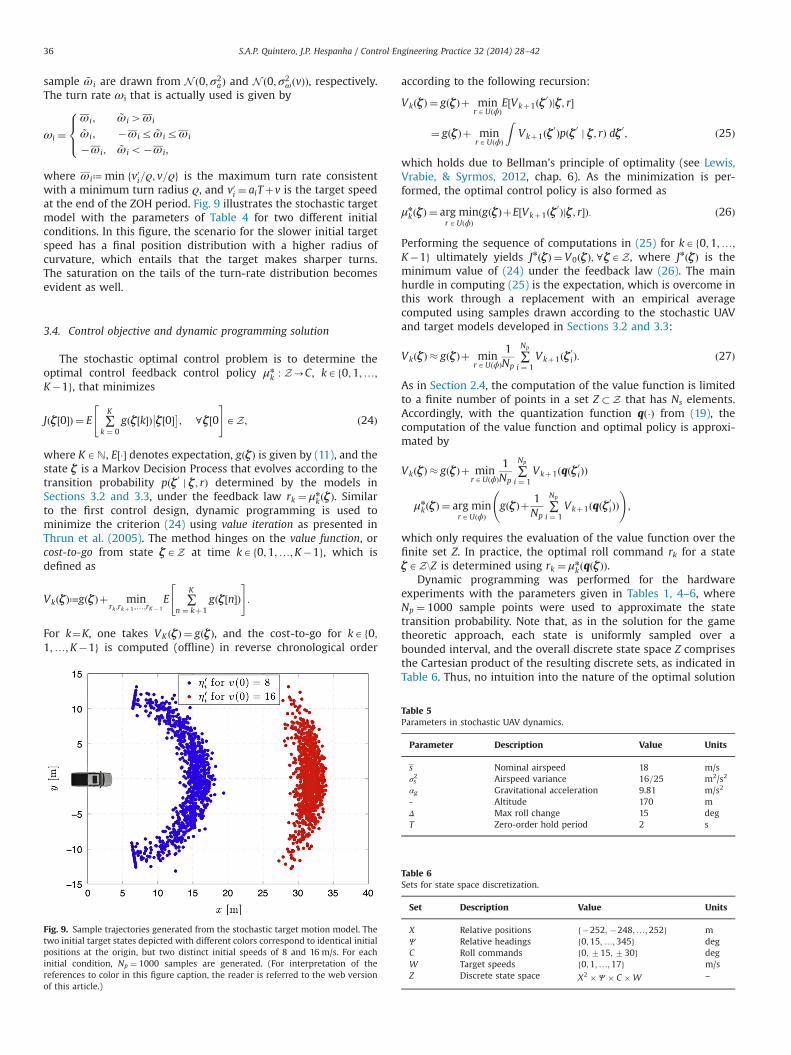
where ω i≔ min fv0i=ϱ; v=ϱg is the maximum turn rate consistentwith a minimum turn radius ϱ, and v0i ¼ aiTþv is the target speedat the end of the ZOH period. Fig. 9 illustrates the stochastic targetmodel with the parameters of Table 4 for two different initialconditions. In this figure, the scenario for the slower initial targetspeed has a final position distribution with a higher radius ofcurvature, which entails that the target makes sharper turns.The saturation on the tails of the turn-rate distribution becomesevident as well.

3.4. Control objective and dynamic programming solution

The stochastic optimal control problem is to determine theoptimal control feedback control policy μn

k : Z-C, kAf0;1;…;

K�1g, that minimizes

Jðζ ½0�Þ ¼ E

"∑K

k ¼ 0gðζ ½k�Þ ζ ½0�

�� �; 8ζ ½0

#AZ; ð24Þ

where KAN, E½�� denotes expectation, gðζÞ is given by (11), and thestate ζ is a Markov Decision Process that evolves according to thetransition probability pðζ 0 j ζ ; rÞ determined by the models inSections 3.2 and 3.3, under the feedback law rk ¼ μn

kðζÞ. Similarto the first control design, dynamic programming is used tominimize the criterion (24) using value iteration as presented inThrun et al. (2005). The method hinges on the value function, orcost-to-go from state ζAZ at time kAf0;1;…;K�1g, which isdefined as

VkðζÞ≔gðζÞþ minrk ;rkþ 1 ;…;rK � 1

E ∑K

n ¼ kþ1gðζ ½n�Þ

" #:

For k¼K, one takes VK ðζÞ ¼ gðζÞ, and the cost-to-go for kAf0;1;…;K�1g is computed (offline) in reverse chronological order

according to the following recursion:

VkðζÞ ¼ gðζÞþ minrAUðϕÞ

E½Vkþ1ðζ 0Þjζ ; r�

¼ gðζÞþ minrAUðϕÞ

ZVkþ1ðζ 0Þpðζ 0 j ζ ; rÞ dζ 0; ð25Þ

which holds due to Bellman's principle of optimality (see Lewis,Vrabie, & Syrmos, 2012, chap. 6). As the minimization is per-formed, the optimal control policy is also formed as

μn

kðζÞ ¼ arg minrAUðϕÞ

ðgðζÞþE½Vkþ1ðζ 0Þjζ ; r�Þ: ð26Þ

Performing the sequence of computations in (25) for kAf0;1;…;

K�1g ultimately yields JnðζÞ ¼ V0ðζÞ; 8ζAZ, where JnðζÞ is theminimum value of (24) under the feedback law (26). The mainhurdle in computing (25) is the expectation, which is overcome inthis work through a replacement with an empirical averagecomputed using samples drawn according to the stochastic UAVand target models developed in Sections 3.2 and 3.3:

VkðζÞ � gðζÞþ minrAUðϕÞ

1Np

∑Np

i ¼ 1Vkþ1ðζ 0iÞ: ð27Þ

As in Section 2.4, the computation of the value function is limitedto a finite number of points in a set Z �Z that has Ns elements.Accordingly, with the quantization function qð�Þ from (19), thecomputation of the value function and optimal policy is approxi-mated by

VkðζÞ � gðζÞþ minrAUðϕÞ

1Np

∑Np

i ¼ 1Vkþ1ðqðζ 0iÞÞ

μn

kðζÞ ¼ arg minrAUðϕÞ

gðζÞþ 1Np

∑Np

i ¼ 1Vkþ1ðqðζ 0iÞÞ

!;

which only requires the evaluation of the value function over thefinite set Z. In practice, the optimal roll command rk for a stateζAZ\Z is determined using rk ¼ μn

kðqðζÞÞ.Dynamic programming was performed for the hardware

experiments with the parameters given in Tables 1, 4–6, whereNp ¼ 1000 sample points were used to approximate the statetransition probability. Note that, as in the solution for the gametheoretic approach, each state is uniformly sampled over abounded interval, and the overall discrete state space Z comprisesthe Cartesian product of the resulting discrete sets, as indicated inTable 6. Thus, no intuition into the nature of the optimal solution

Fig. 9. Sample trajectories generated from the stochastic target motion model. Thetwo initial target states depicted with different colors correspond to identical initialpositions at the origin, but two distinct initial speeds of 8 and 16 m/s. For eachinitial condition, Np ¼ 1000 samples are generated. (For interpretation of thereferences to color in this figure caption, the reader is referred to the web versionof this article.)

Table 5Parameters in stochastic UAV dynamics.

Parameter Description Value Units

s Nominal airspeed 18 m/sσs2 Airspeed variance 16=25 m2/s2

αg Gravitational acceleration 9.81 m/s2

- Altitude 170 mΔ Max roll change 15 degT Zero-order hold period 2 s

Table 6Sets for state space discretization.

Set Description Value Units

X Relative positions f�252; �248;…;252g mΨ Relative headings f0;15;…;345g degC Roll commands f0; 715; 730g degW Target speeds f0;1;…;17g m/sZ Discrete state space X2 � Ψ � C �W –

S.A.P. Quintero, J.P. Hespanha / Control Engineering Practice 32 (2014) 28–4236

is exploited, and the dynamic programming solution to thestochastic optimal control problem remains quite general, requir-ing no additional computational effort even when there are nogimbal constraints, i.e., when λ1 ¼ λ2 ¼ 0 in (12).

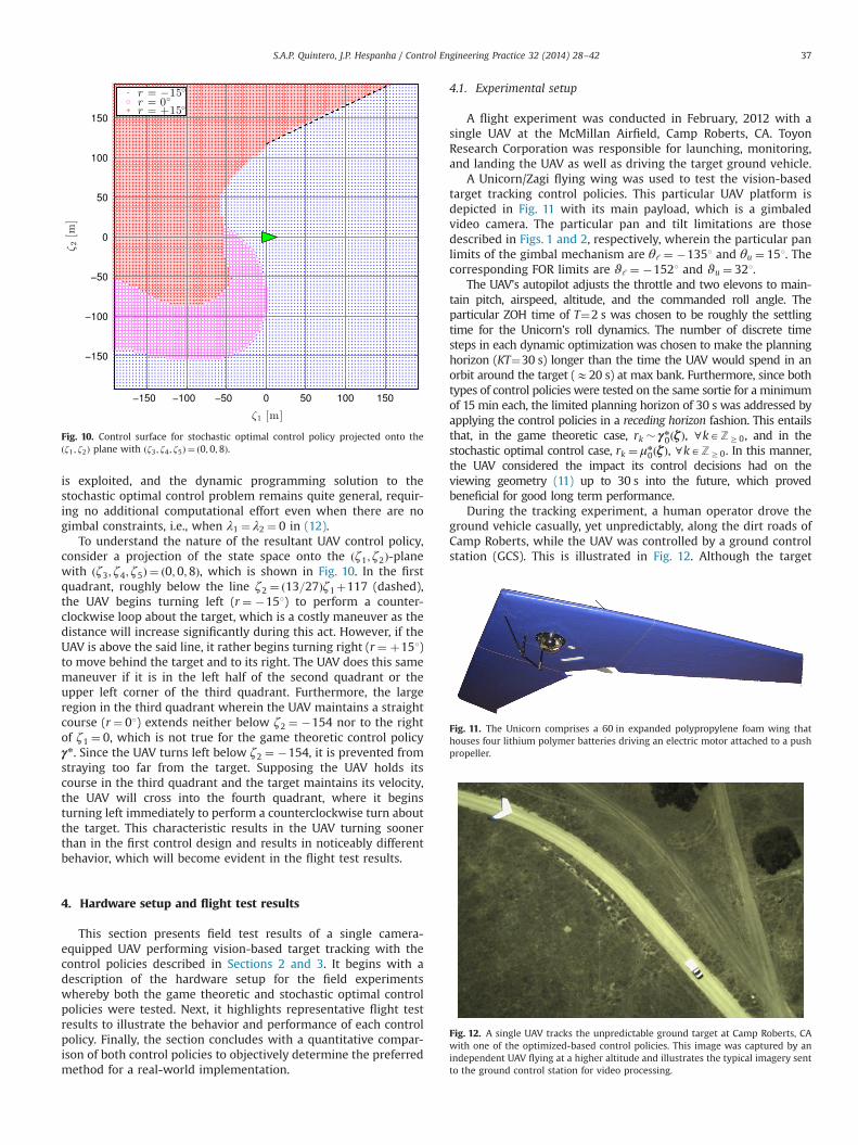
To understand the nature of the resultant UAV control policy,consider a projection of the state space onto the ðζ1; ζ2Þ-planewith ðζ3; ζ4;ζ5Þ ¼ ð0;0;8Þ, which is shown in Fig. 10. In the firstquadrant, roughly below the line ζ2 ¼ ð13=27Þζ1þ117 (dashed),the UAV begins turning left (r¼ �151) to perform a counter-clockwise loop about the target, which is a costly maneuver as thedistance will increase significantly during this act. However, if theUAV is above the said line, it rather begins turning right (r¼ þ151)to move behind the target and to its right. The UAV does this samemaneuver if it is in the left half of the second quadrant or theupper left corner of the third quadrant. Furthermore, the largeregion in the third quadrant wherein the UAV maintains a straightcourse (r¼ 01) extends neither below ζ2 ¼ �154 nor to the rightof ζ1 ¼ 0, which is not true for the game theoretic control policyγn. Since the UAV turns left below ζ2 ¼ �154, it is prevented fromstraying too far from the target. Supposing the UAV holds itscourse in the third quadrant and the target maintains its velocity,the UAV will cross into the fourth quadrant, where it beginsturning left immediately to perform a counterclockwise turn aboutthe target. This characteristic results in the UAV turning soonerthan in the first control design and results in noticeably differentbehavior, which will become evident in the flight test results.

4. Hardware setup and flight test results

This section presents field test results of a single camera-equipped UAV performing vision-based target tracking with thecontrol policies described in Sections 2 and 3. It begins with adescription of the hardware setup for the field experimentswhereby both the game theoretic and stochastic optimal controlpolicies were tested. Next, it highlights representative flight testresults to illustrate the behavior and performance of each controlpolicy. Finally, the section concludes with a quantitative compar-ison of both control policies to objectively determine the preferredmethod for a real-world implementation.

4.1. Experimental setup

A flight experiment was conducted in February, 2012 with asingle UAV at the McMillan Airfield, Camp Roberts, CA. ToyonResearch Corporation was responsible for launching, monitoring,and landing the UAV as well as driving the target ground vehicle.

A Unicorn/Zagi flying wing was used to test the vision-basedtarget tracking control policies. This particular UAV platform isdepicted in Fig. 11 with its main payload, which is a gimbaledvideo camera. The particular pan and tilt limitations are thosedescribed in Figs. 1 and 2, respectively, wherein the particular panlimits of the gimbal mechanism are θℓ ¼ �1351 and θu ¼ 151. Thecorresponding FOR limits are ϑℓ ¼ �1521 and ϑu ¼ 321.

The UAV's autopilot adjusts the throttle and two elevons to main-tain pitch, airspeed, altitude, and the commanded roll angle. Theparticular ZOH time of T¼2 s was chosen to be roughly the settlingtime for the Unicorn's roll dynamics. The number of discrete timesteps in each dynamic optimization was chosen to make the planninghorizon (KT¼30 s) longer than the time the UAV would spend in anorbit around the target (E20 s) at max bank. Furthermore, since bothtypes of control policies were tested on the same sortie for a minimumof 15 min each, the limited planning horizon of 30 s was addressed byapplying the control policies in a receding horizon fashion. This entailsthat, in the game theoretic case, rk � γn

0ðζÞ, 8kAZZ0, and in thestochastic optimal control case, rk ¼ μn

0ðζÞ, 8kAZZ0. In this manner,the UAV considered the impact its control decisions had on theviewing geometry (11) up to 30 s into the future, which provedbeneficial for good long term performance.

During the tracking experiment, a human operator drove theground vehicle casually, yet unpredictably, along the dirt roads ofCamp Roberts, while the UAV was controlled by a ground controlstation (GCS). This is illustrated in Fig. 12. Although the target

Fig. 10. Control surface for stochastic optimal control policy projected onto theðζ1 ; ζ2Þ plane with ðζ3 ; ζ4 ; ζ5Þ ¼ ð0;0;8Þ.

Fig. 11. The Unicorn comprises a 60 in expanded polypropylene foam wing thathouses four lithium polymer batteries driving an electric motor attached to a pushpropeller.

Fig. 12. A single UAV tracks the unpredictable ground target at Camp Roberts, CAwith one of the optimized-based control policies. This image was captured by anindependent UAV flying at a higher altitude and illustrates the typical imagery sentto the ground control station for video processing.

S.A.P. Quintero, J.P. Hespanha / Control Engineering Practice 32 (2014) 28–42 37

remained on the roads for the duration of the tracking experi-ments, this did not benefit the tracking algorithm since the UAV'scontrol policies were computed with no information regardingroad networks. The UAV's control actions were computed usingMATLABs, which communicated with the GCS and the GPSreceiver onboard the truck to acquire the UAV telemetry andtarget data and to determine the roll command according to theparticular control policy being tested on the UAV. The rollcommand was then sent back to the GCS and relayed to the UAV.

In real-world conditions, steady winds are often encounteredhaving speeds that constitute a significant portion of a small UAV'sairspeed. While the policies presented do not address heavy windsthat alter the UAV's kinematics (projected onto the ground)significantly, light to moderate winds can be addressed in anapproximate manner by instead altering the target's apparentground velocity. In particular, Saunders and Beard (2008) notethat a constant target velocity and steady wind can be generalizedto just a steady wind. We take a similar approach and combine thewind and target velocity to form the target's apparent groundvelocity, since the coordinate frame defined by (9) and (10) iscentered on the target. More specifically, denoting the wind bywAR2, one can take the target's apparent heading ψ g and speed vto be the following:

ψ g ¼ atan2ðv sin ψ g�w2; v cos ψ g�w1Þ ð28Þ

v ¼ffiffiffiffiffiffiffiffiffiffiffiffiffiffiffiffiffiffiffiffiffiffiffiffiffiffiffiffiffiffiffiffiffiffiffiffiffiffiffiffiffiffiffiffiffiffiffiffiffiffiffiffiffiffiffiffiffiffiffiffiffiffiffiffiffiffiffiffiffiffiffiffiffiffiffiðv cosψ g�w1Þ2þðv sin ψ g�w2Þ2

q; ð29Þ

where atan2 is the four-quadrant inverse tangent function. Onethen uses ψ g and v in place of ψ g and v in (9) and (10) respectivelyto determine ζ . In reality, wind truly alters the UAV's groundvelocity vgAR2 and hence its groundspeed. More specifically,vg ¼ ðs cos ðψ Þþw1; s sin ðψ Þþw2Þ per the wind triangle (Beard &McLain, 2012). However, since we have planned for a range oftarget speeds and only a single UAV groundspeed, it is convenientto use the preceding transformation, which we shall see is quiteeffective for even moderate wind speeds. Also, note that theheading of the wind does not correspond to the meteorologicaldefinition of wind, i.e., ψw ¼ atan2ðw2;w1Þ is the direction inwhich the wind is blowing rather than the direction from whichit is blowing. Furthermore, an estimate of the wind field w istypically reported by the autopilot of a small UAV and can beaccurate to within 0.5 m/s of the actual wind speed in practicalsettings (Langelaan, Alley, & Neidhoefer, 2011). Moreover, due tothe robustness of the policies to either uncertain or worst-caserelative dynamics between the UAV and target, estimation error inthe wind speed is unlikely to cause any significant degradation inperformance.

While this approximation was employed during the flight tests,its effects were quite negligible, as the average wind speed (asmeasured by the UAV) was less than 0.5 m/s over each 15-minexperiment. Since wind speeds are often greater than those thatwere experienced during this particular experiment, we addressthe issue of the control policies' robustness to steady winds at theend of the section and keep our focus on robustness to unpre-dictable target motion.

4.2. Game theory results

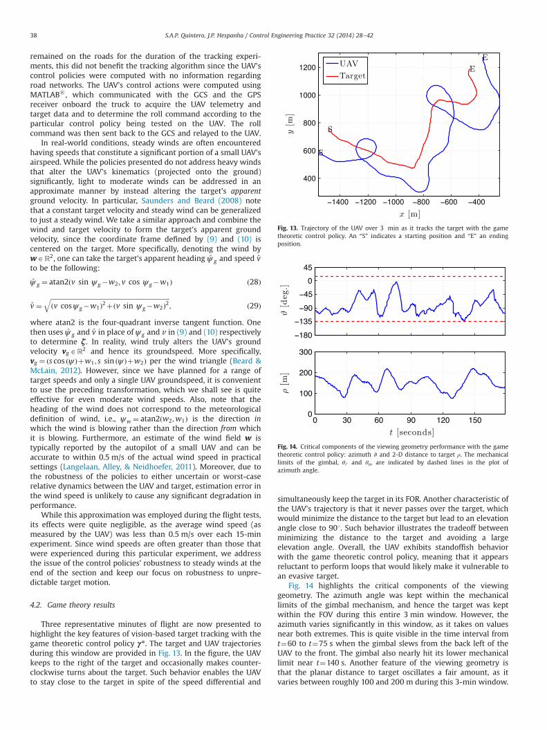
Three representative minutes of flight are now presented tohighlight the key features of vision-based target tracking with thegame theoretic control policy γn. The target and UAV trajectoriesduring this window are provided in Fig. 13. In the figure, the UAVkeeps to the right of the target and occasionally makes counter-clockwise turns about the target. Such behavior enables the UAVto stay close to the target in spite of the speed differential and

simultaneously keep the target in its FOR. Another characteristic ofthe UAV's trajectory is that it never passes over the target, whichwould minimize the distance to the target but lead to an elevationangle close to 901. Such behavior illustrates the tradeoff betweenminimizing the distance to the target and avoiding a largeelevation angle. Overall, the UAV exhibits standoffish behaviorwith the game theoretic control policy, meaning that it appearsreluctant to perform loops that would likely make it vulnerable toan evasive target.

Fig. 14 highlights the critical components of the viewinggeometry. The azimuth angle was kept within the mechanicallimits of the gimbal mechanism, and hence the target was keptwithin the FOV during this entire 3 min window. However, theazimuth varies significantly in this window, as it takes on valuesnear both extremes. This is quite visible in the time interval fromt¼60 to t¼75 s when the gimbal slews from the back left of theUAV to the front. The gimbal also nearly hit its lower mechanicallimit near t¼140 s. Another feature of the viewing geometry isthat the planar distance to target oscillates a fair amount, as itvaries between roughly 100 and 200 m during this 3-min window.

Fig. 13. Trajectory of the UAV over 3 min as it tracks the target with the gametheoretic control policy. An “S” indicates a starting position and “E” an endingposition.

Fig. 14. Critical components of the viewing geometry performance with the gametheoretic control policy: azimuth ϑ and 2-D distance to target ρ. The mechanicallimits of the gimbal, θℓ and θu, are indicated by dashed lines in the plot ofazimuth angle.

S.A.P. Quintero, J.P. Hespanha / Control Engineering Practice 32 (2014) 28–4238

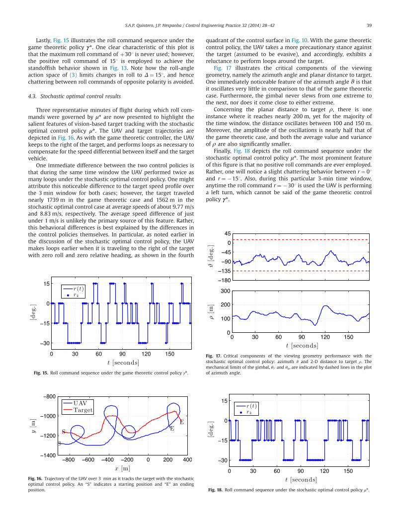
Lastly, Fig. 15 illustrates the roll command sequence under thegame theoretic policy γn. One clear characteristic of this plot isthat the maximum roll command of þ301 is never used; however,the positive roll command of 151 is employed to achieve thestandoffish behavior shown in Fig. 13. Note how the roll-angleaction space of (3) limits changes in roll to Δ¼ 151, and hencechattering between roll commands of opposite polarity is avoided.

4.3. Stochastic optimal control results

Three representative minutes of flight during which roll com-mands were governed by μn are now presented to highlight thesalient features of vision-based target tracking with the stochasticoptimal control policy μn. The UAV and target trajectories aredepicted in Fig. 16. As with the game theoretic controller, the UAVkeeps to the right of the target, and performs loops as necessary tocompensate for the speed differential between itself and the targetvehicle.

One immediate difference between the two control policies isthat during the same time window the UAV performed twice asmany loops under the stochastic optimal control policy. One mightattribute this noticeable difference to the target speed profile overthe 3 min window for both cases; however, the target travelednearly 1739 m in the game theoretic case and 1562 m in thestochastic optimal control case at average speeds of about 9.77 m/sand 8.83 m/s, respectively. The average speed difference of justunder 1 m/s is unlikely the primary source of this feature. Rather,this behavioral differences is best explained by the differences inthe control policies themselves. In particular, as noted earlier inthe discussion of the stochastic optimal control policy, the UAVmakes loops earlier when it is traveling to the right of the targetwith zero roll and zero relative heading, as shown in the fourth

quadrant of the control surface in Fig. 10. With the game theoreticcontrol policy, the UAV takes a more precautionary stance againstthe target (assumed to be evasive), and accordingly, exhibits areluctance to perform loops around the target.

Fig. 17 illustrates the critical components of the viewinggeometry, namely the azimuth angle and planar distance to target.One immediately noticeable feature of the azimuth angle ϑ is thatit oscillates very little in comparison to that of the game theoreticcase. Furthermore, the gimbal never slews from one extreme tothe next, nor does it come close to either extreme.

Concerning the planar distance to target ρ, there is oneinstance where it reaches nearly 200 m, yet for the majority ofthe time window, the distance oscillates between 100 and 150 m.Moreover, the amplitude of the oscillations is nearly half that ofthe game theoretic case, and both the average value and varianceof ρ are also significantly smaller.

Finally, Fig. 18 depicts the roll command sequence under thestochastic optimal control policy μn. The most prominent featureof this figure is that no positive roll commands are ever employed.Rather, one will notice a slight chattering behavior between r¼ 01and r¼ �151. Also, during this particular 3-min time window,anytime the roll command r¼ �301 is used the UAV is performinga left turn, which cannot be said of the game theoretic controlpolicy γn.

Fig. 15. Roll command sequence under the game theoretic control policy γn .

Fig. 16. Trajectory of the UAV over 3 min as it tracks the target with the stochasticoptimal control policy. An “S” indicates a starting position and “E” an endingposition.

Fig. 17. Critical components of the viewing geometry performance with thestochastic optimal control policy: azimuth ϑ and 2-D distance to target ρ. Themechanical limits of the gimbal, θℓ and θu, are indicated by dashed lines in the plotof azimuth angle.

Fig. 18. Roll command sequence under the stochastic optimal control policy μn .

S.A.P. Quintero, J.P. Hespanha / Control Engineering Practice 32 (2014) 28–42 39

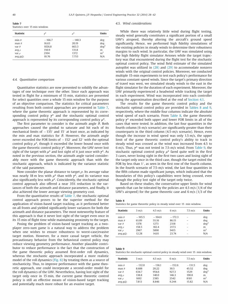
4.4. Quantitative comparison

Quantitative statistics are now presented to solidify the advan-tages of one technique over the other. Since each approach wastested in flight for a minimum of 15 min, statistics are presentedfor select quantities over a whole 15 min window for the purposeof an objective comparison. The statistics for critical parametersresulting from both control approaches are presented in Table 7,where the game theoretic approach is represented by its corre-sponding control policy γn and the stochastic optimal controlapproach is represented by its corresponding control policy μn.

The first parameter to consider is the azimuth angle ϑ. Bothapproaches caused the gimbal to saturate and hit each of itsmechanical limits of �1351 and 151 at least once, as indicated bythe min and max statistics for ϑ. However, the azimuth anglenever exceeded the FOR limits of �1521 and 321 with the optimalcontrol policy μn, though it exceeded the lower bound once withthe game theoretic control policy γn. Moreover, the UAV never lostsight of the target with μn and lost sight of it just once with γn. Asnoted in the previous section, the azimuth angle varied consider-ably more with the game theoretic approach than with thestochastic approach, which is indicated by the variance statisticof the said parameter.

Now consider the planar distance to target ρ. Its average valuewas nearly 18 m less with μn than with γn, and its variance wasalso significantly less with μn. Coincidently, the stochastic optimalcontrol approach also offered a near 35% reduction in the var-iances of both the azimuth and distance parameters, and finally, italso achieved the lower average viewing geometry cost.

From the quantitative results of Table 7, the stochastic optimalcontrol approach proves to be the superior method for theapplication of vision-based target tracking, as it performed betteron all fronts and yielded significantly lower variances for both theazimuth and distance parameters. The most noteworthy feature ofthis approach is that it never lost sight of the target even once inits 15 min of flight time while maintaining proximity to the target.

Posing the problem of vision-based target tracking as a two-player zero-sum game is a natural way to address the problemwhen one wishes to ensure robustness to worst-case/evasivetarget motion. However, for a more casual target vehicle, theprecautionary behavior from the behavioral control policy mayreduce viewing geometry performance. Another plausible contri-butor to reduce performance is the fact that the construction ofthe game theoretic policy assumed first-order roll dynamics,whereas the stochastic approach incorporated a more realisticmodel of the roll dynamics (Fig. 6) by treating them as a source ofstochasticity. Thus, to improve performance with the game theo-retic approach, one could incorporate a second-order model forthe roll dynamics of the UAV. Nevertheless, having lost sight of thetarget only once in 15 min, the current game theoretic controlpolicy is still an effective means of vision-based target trackingand potentially much more robust for an evasive target.

4.5. Wind considerations

While there was relatively little wind during flight testing,steady wind generally constitutes a significant portion of a smallUAV's airspeed, thereby altering the aircraft's ground speedsignificantly. Hence, we performed high fidelity simulations ofthe existing policies in steady winds to determine their robustnessmargins to such wind. In particular, the UAV was simulated usingthe high fidelity flight simulator Aviones while the target trajec-tory was that encountered during the flight test for the stochasticoptimal control policy. The wind field estimate of the simulatedautopilot was utilized in (28) and (29) to accommodate nonzerowinds with the original control policies. Moreover, we conductedmultiple 15-min experiments to test each policy's performance forvarious constant-speed winds. Since the target's primary directionof travel was west, we simulated steady winds to the east in theflight simulator for the duration of each experiment. Moreover, theUAV primarily experienced a headwind while tracking the targetin each experiment. Wind was incorporated into each controllerusing the approximation described at the end of Section 4.1.

The results for the game theoretic control policy and thestochastic optimal control policy are provided in Tables 8 and 9,respectively, where the middle four columns indicate the absolutewind speed of each scenario. From Table 8, the game theoreticpolicy γn exceeded both upper and lower FOR limits in all of thecases that were tested. In addition, the last four quantities in thefourth column (6-m/s scenario) are significantly greater than theircounterparts in the third column (4.5-m/s scenario). Hence, eventhough the increase in wind speed was only 1.5 m/s, the upperlimit of the game theoretic control policy's ability to track insteady wind was crossed as the wind was increased from 4.5 to6 m/s. Thus, γn was not tested in 7.5-m/s wind. From Table 9, thestochastic optimal control policy μn fared quite well in the first3 cases, never losing sight in the first two cases and losing sight ofthe target only once in the third case, though the target exited theFOR by less than 11, as seen in the first row of the fourth column.In the fourth scenario of 7.5-m/s wind, the last four quantities inthe fifth column made significant jumps, which indicated that theboundaries of this policy's capabilities were being crossed, eventhough the policy lost sight of the target only twice.

Based on these studies, the conservative upper limits for windspeeds that can be tolerated by the policies are 4.5 m/s (1/4 of theUAV's airspeed) for the game theoretic case and 6 m/s (1/3 of the

Table 7Statistics over 15 min window.

Statistic γn μn Units

min ϑ �166.7 �140.3 degmax ϑ 16.63 20.19 degvar ϑ 1026.8 663.3 deg2

avg ρ 150.9 131.8 mvar ρ 2104 1372 m2

avg gðζÞ 10.76 7.753 N/A

Table 8Statistics for game theoretic policy in steady wind over 15 min window.

Statistic 3 m/s 4.5 m/s 6 m/s 7.5 m/s Units

min ϑ �165.5 �164.6 �172.3 – degmax ϑ 61.09 55.16 86.15 – degvar ϑ 1378 1273 2318 – deg2

avg ρ 158.5 182.4 217.5 – mvar ρ 2967 5890 9415 – m2

avg gðζÞ 12.28 14.81 23.74 – N/A

Table 9Statistics for stochastic optimal control policy in steady wind over 15 min window.

Statistic 3 m/s 4.5 m/s 6 m/s 7.5 m/s Units

min ϑ �132.0 �136.1 �152.6 �131.5 degmax ϑ 8.688 20.22 30.5 45.52 degvar ϑ 634.7 954.6 927.3 1529 deg2

avg ρ 138.8 140.0 146.3 190.8 mvar ρ 1692 2385 2542 8181 m2

avg gðζÞ 7.813 8.846 9.244 15.82 N/A

S.A.P. Quintero, J.P. Hespanha / Control Engineering Practice 32 (2014) 28–4240

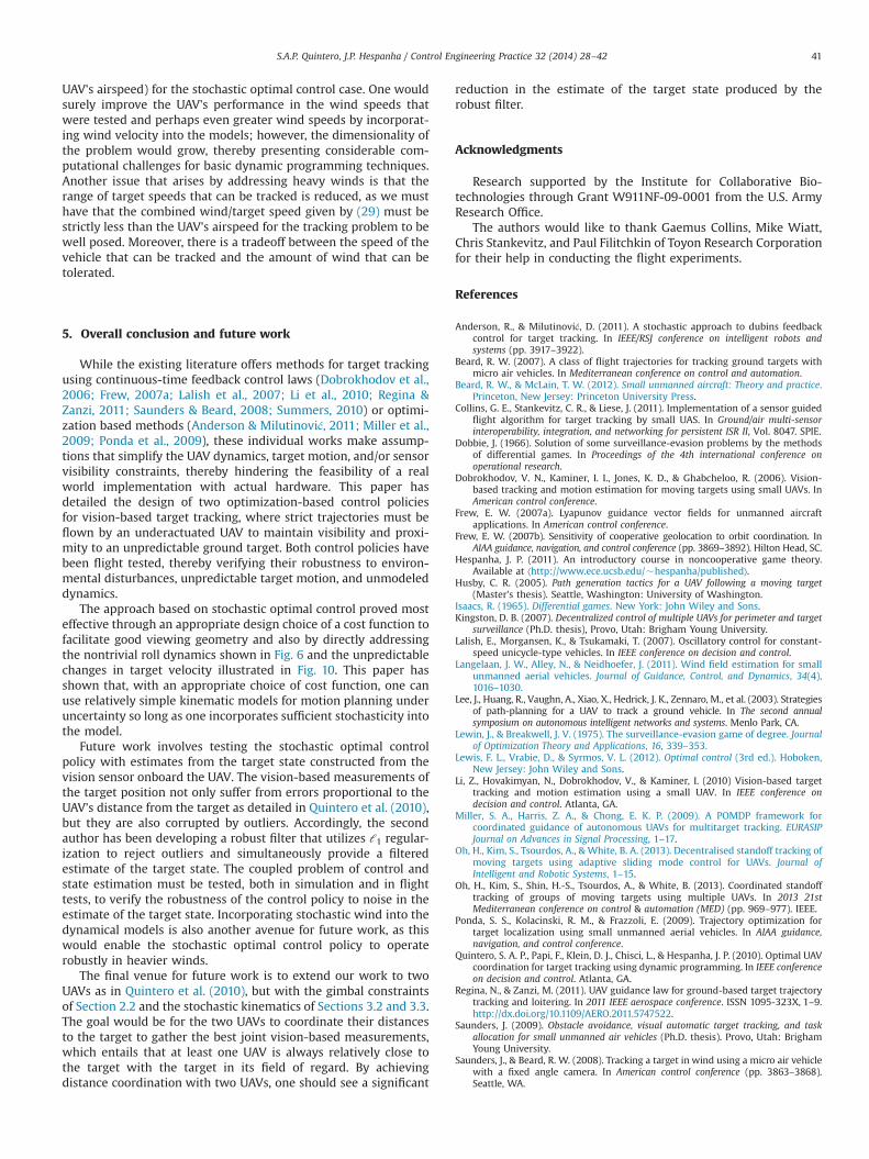
UAV's airspeed) for the stochastic optimal control case. One wouldsurely improve the UAV's performance in the wind speeds thatwere tested and perhaps even greater wind speeds by incorporat-ing wind velocity into the models; however, the dimensionality ofthe problem would grow, thereby presenting considerable com-putational challenges for basic dynamic programming techniques.Another issue that arises by addressing heavy winds is that therange of target speeds that can be tracked is reduced, as we musthave that the combined wind/target speed given by (29) must bestrictly less than the UAV's airspeed for the tracking problem to bewell posed. Moreover, there is a tradeoff between the speed of thevehicle that can be tracked and the amount of wind that can betolerated.

5. Overall conclusion and future work

While the existing literature offers methods for target trackingusing continuous-time feedback control laws (Dobrokhodov et al.,2006; Frew, 2007a; Lalish et al., 2007; Li et al., 2010; Regina &Zanzi, 2011; Saunders & Beard, 2008; Summers, 2010) or optimi-zation based methods (Anderson & Milutinović, 2011; Miller et al.,2009; Ponda et al., 2009), these individual works make assump-tions that simplify the UAV dynamics, target motion, and/or sensorvisibility constraints, thereby hindering the feasibility of a realworld implementation with actual hardware. This paper hasdetailed the design of two optimization-based control policiesfor vision-based target tracking, where strict trajectories must beflown by an underactuated UAV to maintain visibility and proxi-mity to an unpredictable ground target. Both control policies havebeen flight tested, thereby verifying their robustness to environ-mental disturbances, unpredictable target motion, and unmodeleddynamics.

The approach based on stochastic optimal control proved mosteffective through an appropriate design choice of a cost function tofacilitate good viewing geometry and also by directly addressingthe nontrivial roll dynamics shown in Fig. 6 and the unpredictablechanges in target velocity illustrated in Fig. 10. This paper hasshown that, with an appropriate choice of cost function, one canuse relatively simple kinematic models for motion planning underuncertainty so long as one incorporates sufficient stochasticity intothe model.

Future work involves testing the stochastic optimal controlpolicy with estimates from the target state constructed from thevision sensor onboard the UAV. The vision-based measurements ofthe target position not only suffer from errors proportional to theUAV's distance from the target as detailed in Quintero et al. (2010),but they are also corrupted by outliers. Accordingly, the secondauthor has been developing a robust filter that utilizes ℓ1 regular-ization to reject outliers and simultaneously provide a filteredestimate of the target state. The coupled problem of control andstate estimation must be tested, both in simulation and in flighttests, to verify the robustness of the control policy to noise in theestimate of the target state. Incorporating stochastic wind into thedynamical models is also another avenue for future work, as thiswould enable the stochastic optimal control policy to operaterobustly in heavier winds.

The final venue for future work is to extend our work to twoUAVs as in Quintero et al. (2010), but with the gimbal constraintsof Section 2.2 and the stochastic kinematics of Sections 3.2 and 3.3.The goal would be for the two UAVs to coordinate their distancesto the target to gather the best joint vision-based measurements,which entails that at least one UAV is always relatively close tothe target with the target in its field of regard. By achievingdistance coordination with two UAVs, one should see a significant

reduction in the estimate of the target state produced by therobust filter.

Acknowledgments

Research supported by the Institute for Collaborative Bio-technologies through Grant W911NF-09-0001 from the U.S. ArmyResearch Office.

The authors would like to thank Gaemus Collins, Mike Wiatt,Chris Stankevitz, and Paul Filitchkin of Toyon Research Corporationfor their help in conducting the flight experiments.

References

Anderson, R., & Milutinović, D. (2011). A stochastic approach to dubins feedbackcontrol for target tracking. In IEEE/RSJ conference on intelligent robots andsystems (pp. 3917–3922).

Beard, R. W. (2007). A class of flight trajectories for tracking ground targets withmicro air vehicles. In Mediterranean conference on control and automation.

Beard, R. W., & McLain, T. W. (2012). Small unmanned aircraft: Theory and practice.Princeton, New Jersey: Princeton University Press.

Collins, G. E., Stankevitz, C. R., & Liese, J. (2011). Implementation of a sensor guidedflight algorithm for target tracking by small UAS. In Ground/air multi-sensorinteroperability, integration, and networking for persistent ISR II, Vol. 8047. SPIE.

Dobbie, J. (1966). Solution of some surveillance-evasion problems by the methodsof differential games. In Proceedings of the 4th international conference onoperational research.

Dobrokhodov, V. N., Kaminer, I. I., Jones, K. D., & Ghabcheloo, R. (2006). Vision-based tracking and motion estimation for moving targets using small UAVs. InAmerican control conference.

Frew, E. W. (2007a). Lyapunov guidance vector fields for unmanned aircraftapplications. In American control conference.

Frew, E. W. (2007b). Sensitivity of cooperative geolocation to orbit coordination. InAIAA guidance, navigation, and control conference (pp. 3869–3892). Hilton Head, SC.

Hespanha, J. P. (2011). An introductory course in noncooperative game theory.Available at ⟨http://www.ece.ucsb.edu/�hespanha/published⟩.

Husby, C. R. (2005). Path generation tactics for a UAV following a moving target(Master's thesis). Seattle, Washington: University of Washington.

Isaacs, R. (1965). Differential games. New York: John Wiley and Sons.Kingston, D. B. (2007). Decentralized control of multiple UAVs for perimeter and target

surveillance (Ph.D. thesis), Provo, Utah: Brigham Young University.Lalish, E., Morgansen, K., & Tsukamaki, T. (2007). Oscillatory control for constant-

speed unicycle-type vehicles. In IEEE conference on decision and control.Langelaan, J. W., Alley, N., & Neidhoefer, J. (2011). Wind field estimation for small

unmanned aerial vehicles. Journal of Guidance, Control, and Dynamics, 34(4),1016–1030.

Lee, J., Huang, R., Vaughn, A., Xiao, X., Hedrick, J. K., Zennaro, M., et al. (2003). Strategiesof path-planning for a UAV to track a ground vehicle. In The second annualsymposium on autonomous intelligent networks and systems. Menlo Park, CA.

Lewin, J., & Breakwell, J. V. (1975). The surveillance-evasion game of degree. Journalof Optimization Theory and Applications, 16, 339–353.

Lewis, F. L., Vrabie, D., & Syrmos, V. L. (2012). Optimal control (3rd ed.). Hoboken,New Jersey: John Wiley and Sons.

Li, Z., Hovakimyan, N., Dobrokhodov, V., & Kaminer, I. (2010) Vision-based targettracking and motion estimation using a small UAV. In IEEE conference ondecision and control. Atlanta, GA.

Miller, S. A., Harris, Z. A., & Chong, E. K. P. (2009). A POMDP framework forcoordinated guidance of autonomous UAVs for multitarget tracking. EURASIPJournal on Advances in Signal Processing, 1–17.

Oh, H., Kim, S., Tsourdos, A., & White, B. A. (2013). Decentralised standoff tracking ofmoving targets using adaptive sliding mode control for UAVs. Journal ofIntelligent and Robotic Systems, 1–15.

Oh, H., Kim, S., Shin, H.-S., Tsourdos, A., & White, B. (2013). Coordinated standofftracking of groups of moving targets using multiple UAVs. In 2013 21stMediterranean conference on control & automation (MED) (pp. 969–977). IEEE.

Ponda, S. S., Kolacinski, R. M., & Frazzoli, E. (2009). Trajectory optimization fortarget localization using small unmanned aerial vehicles. In AIAA guidance,navigation, and control conference.

Quintero, S. A. P., Papi, F., Klein, D. J., Chisci, L., & Hespanha, J. P. (2010). Optimal UAVcoordination for target tracking using dynamic programming. In IEEE conferenceon decision and control. Atlanta, GA.

Regina, N., & Zanzi, M. (2011). UAV guidance law for ground-based target trajectorytracking and loitering. In 2011 IEEE aerospace conference. ISSN 1095-323X, 1–9.http://dx.doi.org/10.1109/AERO.2011.5747522.

Saunders, J. (2009). Obstacle avoidance, visual automatic target tracking, and taskallocation for small unmanned air vehicles (Ph.D. thesis). Provo, Utah: BrighamYoung University.

Saunders, J., & Beard, R. W. (2008). Tracking a target in wind using a micro air vehiclewith a fixed angle camera. In American control conference (pp. 3863–3868).Seattle, WA.

S.A.P. Quintero, J.P. Hespanha / Control Engineering Practice 32 (2014) 28–42 41

Stachura, M., Carfang, A., & Frew, E. W. (2009). Cooperative target tracking with acommunication limited active sensor network. In International workshop onrobotic wireless sensor networks. Marina Del Ray, CA.

Summers, T. H. (2010). Cooperative shape and orientation control of autonomousvehicle formations (Ph.D. thesis), Austin, Texas: University of Texas at Austin.

Thrun, S., Burgard, W., & Fox, D. (2005). Probabilistic robotics. Cambridge, Massa-chusetts: The MIT Press.

URL: ⟨http://aviones.sourceforge.net⟩, 2007.Wheeler, M., Schrick, B., Whitacre, W., Campbell, M., Rysdyk, R. T., & Wise, R. A.

(2006). Cooperative tracking of moving targets by a team of autonomous UAVs.In IEEE/AIAA 25th digital avionics systems conference.

S.A.P. Quintero, J.P. Hespanha / Control Engineering Practice 32 (2014) 28–4242