ABSTRACT

Title of Thesis: MODELING UNCERTAINTY IN RAIL

FREIGHT OPERATIONS: IMPLICATIONS FOR

SERVICE RELIABILITY.

Degree Candidate: Vishnu Charan Arcot

Degree and Year Master of Science, 2007

Directed By: Professor Hani S. Mahmassani Department of Civil & Environmental Engineering

This thesis presents an operational simulation tool to evaluate different rail

operational policies aimed at increasing service reliability in large-scale multi-carrier

rail networks. Operational policies that improve shipment connection reliability at

shunting yards, such as priority-based classification, train holding and train

cancellation policies can be evaluated using the tool. To support operational decisions

needed to implement priority-based classification, an optimization based framework

is proposed. Operational policies to improve train schedule reliability, such as

including slack time in timetables to handle minor delays, and rescheduling strategies

to manage large delays can also be evaluated using the tool. For minor delays, an

analytical method for deterministic analysis of propagation of delays in train traffic

networks is proposed and demonstrated on the Washington DC Metrorail Network.

Rescheduling strategies required to manage large delays in multi-carrier rail networks

are also discussed herein. A dynamic slot request mechanism is proposed, wherein

each carrier requests slots for N blocks ahead, to model rescheduling requests of

multiple carriers competing for the slots. The proposed simulation tool is applied on a

European rail freight network, the REORIENT network, to evaluate the effect of

variability in border crossing times, slack time in timetable design, different

rescheduling policies and slot request size (N) on service reliability and average delay

to the trains in the system.

MODELING UNCERTAINTY IN RAIL FREIGHT OPERATIONS: IMPLICATIONS FOR SERVICE

RELIABILITY

By

Vishnu Charan Arcot

Thesis submitted to the Faculty of the Graduate School of the University of Maryland, College Park, in partial fulfillment

of the requirements for the degree of Master of Science

2007

Advisory Committee:

Professor Hani S. Mahmassani, Chair Professor Paul M. Schonfeld Associate Professor Elise Miller-Hooks

© Copyright by

Vishnu Charan Arcot

2007

ii

Dedication

To Bapa, Amma, Malli and Guru

iii

Acknowledgements

First and foremost, I would like to thank my advisor, Dr. Hani Mahmassani,

for his guidance, support and encouragement. I am grateful to him for the knowledge

I gained from him in Transportation Engineering and otherwise. He has always

inspired me to do my best. I also thank Dr. Schonfeld and Dr. Miller-Hooks for

serving on my committee. I am grateful to Dr. Miller-Hooks for the things I learnt

from her in the Reorient project.

I would like to thank my colleagues and office-mates at UMD for their advice,

help and friendship. I have learnt a great deal from many of my colleagues and am

indebted to them for the wonderful time I shared with them. I would also like to thank

my friends in Greenbelt for making my stay enjoyable and comfortable.

I would especially like to thank my parents, brother and sister for their moral

support and encouragement. They have continuously supported me throughout my

graduate studies and motivated me whenever I needed it. I dedicate this thesis to them.

iv

Table of Contents

Dedication ..................................................................................................................... ii

Acknowledgements...................................................................................................... iii

Table of Contents......................................................................................................... iv

List of Tables ............................................................................................................. viii

List of Figures .............................................................................................................. ix

Chapter 1: Introduction ................................................................................................ 1

1.1 Motivation........................................................................................................... 1

1.2 Rail Service Reliability ....................................................................................... 2

1.3 Shipment Connection Reliability........................................................................ 3

1.4 Train Schedule Reliability .................................................................................. 4

1.4.1 Slack in timetables ....................................................................................... 5

1.4.2 Rescheduling Strategies ............................................................................... 5

1.5 Performance Measures........................................................................................ 6

1.6 Thesis Objective.................................................................................................. 9

1.7 Structure of the Thesis ...................................................................................... 10

Chapter 2: Modeling Uncertainty in Shipment Connections..................................... 12

2.1 Introduction....................................................................................................... 12

2.1.1 Current Car Scheduling Practice................................................................ 13

2.1.2 Rail Yard Operations ................................................................................. 15

2.1.2.1 Receiving and departure ..................................................................... 15

2.1.2.2 Classification and assembly................................................................ 16

v

2.1.2.3 Connection delay ................................................................................ 16

2.1.3 Dynamic Car Scheduling ........................................................................... 18

2.1.4 Priority Based Classification...................................................................... 18

2.2 Modeling Yard Operations ............................................................................... 19

2.2.1 Literature Review....................................................................................... 19

2.2.2 Bulk queueing model and its applications ................................................. 22

2.3 Modeling Priority-based Classification ............................................................ 25

2.3.1 Previous Studies......................................................................................... 26

2.3.2. Hump Sequencing Algorithm ................................................................... 29

2.3.3. Dynamic Block to Track Assignment....................................................... 31

2.3.3.1 Management of Rehump Activities .................................................... 32

2.3.3.2 Fitting Blocks into Available Track Space ......................................... 38

2.4 Summary and Conclusions ............................................................................... 45

Chapter 3: Modeling Uncertainty in Schedule Adherence: Minor Delays ................. 47

3.1 Introduction....................................................................................................... 47

3.1.1 Rail Traffic Characteristics ........................................................................ 48

3.2 Literature on delay propagation in rail networks.............................................. 49

3.2.1 Deterministic model for delay propagation– Max-Plus Algebra............... 49

3.2.2 Stochastic models for delay propagation ................................................... 52

3.3 Network Preparation ......................................................................................... 54

3.3.1 Network Building....................................................................................... 55

3.3.2 Slack Times in Timetable Design: Unstable timetables; Unrealizable

timetables ............................................................................................................ 57

vi

3.4 Delay Propagation in Train Networks .............................................................. 59

3.4.1 Example passenger network ...................................................................... 59

3.5 Delay Propagation Algorithm........................................................................... 64

3.5.1 Longest path algorithm .............................................................................. 65

3.6 Stability Analysis .............................................................................................. 68

3.6.1 Critical Train.............................................................................................. 70

3.6 Summary and Conclusions ............................................................................... 70

Chapter 4: Modeling Uncertainty in Schedule Adherence: Large Delays................. 72

4.1 Introduction....................................................................................................... 72

4.1.1 Conflict Management Policies................................................................... 72

4.2 Related Works in Conflict Management........................................................... 73

4.3 Framework for Rescheduling in Multi-Carrier Rail Networks......................... 75

4.3.1 Dynamic Slot Request Mechanism............................................................ 76

4.3.2 Trade-offs in Selecting the value of Slot Request Size (N) ....................... 77

4.3.3 Slot Reservation ......................................................................................... 78

4.3.4 Train Simulation ........................................................................................ 80

4.3.4 Conflict Detection...................................................................................... 80

4.3.5 Conflict Resolution .................................................................................... 82

4.3.5.1 Resolution Measures........................................................................... 83

4.3.5.2 Look Ahead Method ........................................................................... 85

4.4 Application: REORIENT Network................................................................... 87

4.5 Design of Experiments...................................................................................... 90

4.5.1 The Base Case: Scenario 1......................................................................... 90

vii

4.5.2 Variability in Delays at Borders ................................................................ 91

4.5.3 Slack Time in Timetable Design................................................................ 93

4.5.4 Rescheduling Policy................................................................................... 94

4.5.5 Slot Request Size (N)................................................................................. 95

4.6 Discussion of Results........................................................................................ 96

4.6.1 Effect of Variability in Border Delays....................................................... 96

4.6.1.1 Effect of Variability in border delays on Total Delay in the System.. 96

4.6.1.2 Effect of Variability in border delays on Service Reliability ............. 97

4.6.1.3 Effect of Variability in border delays on Service Desirability ........... 98

4.6.2 Effect of Slack Time in Timetable Design ................................................ 99

4.6.2.1 Effect of Slack Time on Average Delay in the System ...................... 99

4.6.2.2 Effect of Slack Time on Rail Punctuality and Service Reliability.... 100

4.6.2.3 Effect of Slack Time: Trade-off between Stability of train network and

Frequency of Service offered........................................................................ 102

4.6.3 Effect of Rescheduling Policy ................................................................. 104

4.6.4 Effect of Slot Request Size (N)................................................................ 105

4.6 Summary and Conclusions ............................................................................. 106

Chapter 5: Conclusions ........................................................................................... 109

5.1 Introduction..................................................................................................... 109

5.2 Summary and Contributions ........................................................................... 109

5.3 Limitations and Directions for Future Research............................................. 113

Appendices................................................................................................................ 114

Bibliography ............................................................................................................. 116

viii

List of Tables

Table 1: Connection Matrix by Train Block............................................................... 33

Table 2: Connection Matrix after Rehump ................................................................. 34

Table 3: Different Rehumping Scenarios ................................................................... 35

Table 4: Decision Variables for Management of Rehump Activities Problem .......... 36

Table 5: Result - Management of Rehump Activities ................................................ 37

Table 6: Input to Block-to-Track Assignment Step.................................................... 40

Table 7: Penalties Associated with the type of Assignment ....................................... 40

Table 8: Result from Block to Track Assignment ...................................................... 44

Table 9: Trim-out times of train blocks ...................................................................... 44

Table 10: Route details for the proposed Services on REORIENT Corridor ............. 89

Table 11: Overview of Scenarios tested in Experiments ............................................ 95

Table 12: Mean and Variance of Border Delay Distributions .................................... 96

Table 13: Effect of Variability in Border Delays on Train Delays............................. 97

Table 14: Service Reliability for Border-delay Levels 1 & 3..................................... 98

Table 15: Service Desirability vs. Variability in Border Delays ................................ 99

Table 16: Slack in Timetable vs. Service Reliability................................................ 101

Table 17: Service Desirability vs. Slack Time.......................................................... 103

Table 18: Average Delay to Train for Different Values of N................................... 106

ix

List of Figures

Figure 1: Shipment flow process in Shunting yard..................................................... 15

Figure 2: Bulk Queueing Model ................................................................................. 22

Figure 3: Framework to Implement Priority-based Classification ............................. 29

Figure 4: Train Service Networks with Schedules ..................................................... 55

Figure 5: Train traffic network representation with minimum process times and

headways..................................................................................................................... 57

Figure 6: Train traffic network with slack times ........................................................ 58

Figure 7: WMATA Metrorail Network ...................................................................... 61

Figure 8: Metrorail Network with Slack Times in Period 1 ....................................... 62

Figure 9: Iterative Structure of Metrorail Network..................................................... 63

Figure 10: Delay propagation in the first period......................................................... 67

Figure 11: Delay Amplitudes for the Blue Line ......................................................... 69

Figure 12: Delay Amplitudes for the Orange Line ..................................................... 69

Figure 13: Delay Amplitudes for the Yellow Line ..................................................... 69

Figure 14: Slot Reservation Process ........................................................................... 79

Figure 15: Train Simulation........................................................................................ 81

Figure 16: Conflict Detection embedded in Train Moving ........................................ 82

Figure 17: The REORIENT Corridor ......................................................................... 89

Figure 18: Border Stations on the Reorient Corridor.................................................. 91

Figure 19: Uniform (15-120) Distribution to Model Border Delays .......................... 92

Figure 20: Uniform Distribution (30-90) to Model Border Delays ............................ 92

Figure 21: Triangular Distribution to Model Border Delays ...................................... 93

x

Figure 22: Effect of Variability in Border Delays on Total Delay in the System ...... 97

Figure 23: Effect of Reducing Variability from Level 1 to Level 3 on Service

Reliability.................................................................................................................... 98

Figure 24: Comparing Service Desirability for Different Levels of Variability in

Border Delays ............................................................................................................. 99

Figure 25: The effect of Slack Time on Average Delay in the System ................... 100

Figure 26: Rail Punctuality vs. Slack Time in Timetable......................................... 100

Figure 27: The effect of Slack Time on Service Reliability ..................................... 101

Figure 28: The effect of Slack time on the number of scheduled trains in the system

................................................................................................................................... 102

Figure 29: The Effect of Slack time on Shipment Ton-Km Attracted by Four Services

................................................................................................................................... 103

Figure 30: Service Desirability vs. Slack Time ........................................................ 104

Figure 31: Effect of Rescheduling Policy on Average Delay to Trains in the System

................................................................................................................................... 105

Figure 32: The effect of Slot Request Size on Average Delay in the System .......... 106

1

Chapter 1:

Introduction

1.1 Motivation

The success of rail freight industry is greatly dependent on the ability of railroads to

deliver reliable service to the customers. Due to the nature of new industries and

businesses, freight shippers today require on-time deliveries and predictable lead

times for ordering goods. According to a market study (Hertenstein and Kaplan, 1991)

cited in Hallowell and Harker (1998), a 1% improvement in the reliability of cargo

delivery time could yield as much as a 5% revenue increase in several markets.

Railroads have trouble delivering consistent and reliable service many customers

require, resulting in significant loss in market share. In Europe, for example, rail

market share for freight transportation dropped from 21% in 1970 to 8.4% in 1998

(EC 2001). The corresponding increase in road market share has negative socio-

environmental impacts due to road congestion (Eurostat 2007). For this reason,

several countries - European Union (EU) in particular - have a vision for an increased

use of railroads for freight transport. Moreover, as a consequence of the emergence of

the intermodal industry, railroads can potentially attract high-valued commodity

markets that are primarily being served by road-based transport. While road transport

has the benefits of immediacy, flexibility and better access to terminals, rail transport

offers a lower cost alternative for multiple loads carried over longer transits and has a

much less polluting effect on the environment. Due to the potential benefits of

promoting rail freight industry, the EU is taking several initiatives like planning

2

dedicated international rail freight corridors, liberalizing rail freight market by

allowing private train operators (carriers) to compete with the state-owned rail

companies. Several operational policies may also need to be adopted to make

railroads more competitive and reliable. This thesis presents an operational simulation

tool to evaluate different rail operational policies aimed at increasing service

reliability in large-scale multi-carrier rail networks.

1.2 Rail Service Reliability

Rail service reliability can be defined from the perspective of carriers or from that of

shippers. A carrier responsible for a particular rail service may be interested in the

likelihood that the trains belonging to the service can be operated according to a pre-

planned schedule, which can be termed as train schedule reliability. Some of the

primary sources of train schedule reliability problems are unexpected events, such as

long border station delays, unavailability of crew, rolling stock or locomotives. In a

highly interconnected rail traffic network, trains share infrastructure with several

other trains and so a delayed train may cause a domino effect of secondary delays

over the entire network.

A shipper, on the other hand, may be interested in the likelihood that a shipment

reaches its destination at the desired time. The shipper may then choose rail transport

depending on shipment connection reliability, which is the likelihood that the

shipment makes all the scheduled train connections required to reach its destination at

the desired time. Shipments may miss their scheduled train connections due to train

delays or variability in yard operating times. Factors affecting shipment connection

3

reliability and train schedule reliability are discussed further in the sections that

follow.

1.3 Shipment Connection Reliability

The main sources of uncertainty in shipment connections are train delays and

unexpected delays in yard operations. Trains arriving at shunting yards consist of cars

intended for many destinations, which are sorted in the yards to depart in appropriate

outbound trains. Shipments belonging to a delayed train might be likely to miss their

scheduled connections at shunting yard. In such situations, the outbound train may be

put on hold so that the shipments of the delayed inbound trains can make their

connection. Such train holding strategies can improve shipment connection reliability.

Another source of uncertainty in shipment connections is the variability in yard

operating times. Due to the nature of operations in yards, rail cars spend large amount

of time in classification yards. The time required for various operations at rail yards

constitute nearly 77% of the origin-to-destination trip times on an average in US

(Turnquist, 1982). Unexpected delays in yard operations may cause some shipments

to miss their connections. In the likelihood of such situations, priority based

classification - as proposed by Kraft (2002) - can improve shipment connection

reliability. The goal of priority based classification is to protect the connections of

high priority shipments. Shipment priority is decided based on the available slack

time with respect to the promised delivery time of the shipments. Adopting

operational policies, such as train holding and priority based classification, can

improve shipment connection reliability which will in turn help make rail freight

transport reliable and competitive. Hence, there is a need for a tool to evaluate the

4

impact of various operational policies aimed at improving shipment connection

reliability in large rail networks.

1.4 Train Schedule Reliability

Unexpected events like long border stations delays cause trains to deviate from the

pre-planned schedule. Due to safety considerations, a delayed train can cause

secondary delays to other trains in the network that share the same infrastructure.

Trains that share the same infrastructure need to maintain safe headway distance in

order to avoid collision. Trains are uniquely susceptible to collision because they run

on fixed rails and are not capable of avoiding a collision by steering away like a road

vehicle. Also trains cannot decelerate rapidly, and are frequently operating at speeds

where, by the time the driver can see an obstacle, the train cannot stop in time to

avoid colliding with it. Hence, an external signal control system is used in practice to

maintain safe headway distance between trains and avoid collisions. The safety

system that is most commonly used is the line blocking system. This safety system

permits only one train at a time to use each (block) track section. Train timetables are

constructed by allocating start and end times (slots) to the trains for access to the

different sections or blocks that each train will traverse such that no other train

occupies the same block at the same time. The timetables are designed to contain

slack in order to recover from minor delays. Slack time is generally incorporated in

train running times, headway between trains and in dwell times at stations.

5

1.4.1 Slack in timetables

Slack time in timetables absorb minor delays and limit the propagation of delays in

the network. As the amount of slack in timetables is increased, the train network

becomes more stable. The stability of rail networks can be defined as the ability to

recover to the original schedule after disruptions to the schedule. In a stable system,

delays settle faster and the rail service is more reliable. Thus, the more the slack

included in timetables, the faster the delays settle. However, increasing slack in

timetables reduces the number of trains that can be scheduled in the network, which

in turn reduces the infrastructure capacity utilization. Infrastructure managers wish to

increase capacity utilization to make more profits. Hence, there exists a trade-off

between capacity utilization and the stability of train traffic networks. There is also a

need for a tool to examine this trade-off.

1.4.2 Rescheduling Strategies

Minor delays are handled by slack in timetables, but major delays disturb the original

schedule to a large extent and require rescheduling strategies. A delayed train may

lose its previously assigned slots to access the tracks in its path. Initial track

allocation may not be possible to retain, resulting in conflicting access requests.

These conflicts may need to be resolved by allocating new slots to each affected train.

For each conflict, there exist two possible resolutions – delaying one train versus

another. Each resolution may result in future conflicts or invalidate conflicts

considered in the initial timetable. This results in large number of interconnected

alternatives and makes the railway traffic networks quite sensitive to disruptions. The

future consequences of the disruptions for the traffic are heavily dependent on the

6

rescheduling strategies or the way conflicts are resolved. A dispatcher, who is

responsible to resolve conflicts, often bases the rescheduling decision on basic

priority of trains in conflict. Passenger trains are given more priority over long-

distance freight trains, which in turn may be given more priority over short-distance

freight trains. However, such policies tend to be myopic as they do not consider the

secondary consequences of rescheduling decisions. The decision of delaying one train

versus another may be made by comparing the total network delay caused by the

trains in conflict. However, delay to some trains may be more costly than delay to

others, especially in multi-carrier networks. Multiple carriers may offer different rail

services, which share the same infrastructure but carry shipments of different values

of time. This is true in the European context, where rail market is partly or fully

deregulated. One (public or private) agent is made responsible for the infrastructure

while independent firms operate the trains. Multiple carriers may compete for slots on

shared track segments. Rescheduling decisions in multi-carrier contexts need to be

made by considering the interests of all stakeholders. Different rescheduling

strategies may result in different levels of service reliability and so there exists a need

for a tool to test different strategies.

1.5 Performance Measures

There is also a need to develop performance measures to evaluate the quality

of different operational policies. The measures need to reflect the performance of the

system from the perspective of both the train operators and the shippers. The

7

following are some of the performance measures that may be used to evaluate

different policies:

• Service reliability: Reliability of a service can be estimated as the percentage

of trains belonging to the service that reach their destination at the scheduled

time.

• Rail punctuality: Rail punctuality can be measured as the percentage of trains

in the network that reach their destination at the scheduled time. This measure

can be used to compare different rescheduling policies. However, punctuality

in itself does not indicate the magnitude of delays experienced by trains and

the related stability of rail traffic networks.

• Total delay: The difference between actual arrival time of a train and

scheduled arrival time is termed as delay. Total delay refers to the sum of

delays to all the trains in the network. This measure reflects the stability of

the train traffic system.

• Number of scheduled trains: The number of scheduled trains in the system is

an indicator of infrastructure capacity utilization, and is of interest to the

infrastructure manager. As the amount of (headway) slack in the timetable is

increased, the number of scheduled trains in the system decreases.

• Average delay: Total delay averaged over all the delayed trains in the network

is referred to as average delay. This measure is an alternate indicator of the

stability of the system, which takes into account the number of trains in the

system.

8

Increasing slack in the timetable may be beneficial from the perspective of train

operator since it can increase service reliability and decrease average delay. However,

increasing slack may also limit the service frequency that the operator can offer. This

may affect the volume of shipments carried by the service as the shippers may not

prefer low frequency service. The following measures reflect the performance of

policies from the perspective of shippers.

• Service desirability: The shipment ton-km attracted by a service reflects the

desirability of that service.

• Rail mode share: Rail mode share refers to the fraction of total demand

attracted by rail. This measure reflects the effect of various policies on rail

competitiveness.

• Shipment travel time reliability: The travel times of the shipments that are

generated in a particular time interval and that travel between a particular

origin-destination pair on rail can be analyzed to estimate the variance. The

variance of the travel times thus estimated is a measure of shipment travel

time reliability. This measure can be used to estimate the effectiveness of

policies to improve shipment connection reliability such as train holding

strategies and priority-based classification method.

9

1.6 Thesis Objective

The objective of this thesis is to present a simulation tool that can support the

evaluation of the following:

• Operational policies at a shunting yard such as train holding, priority-based

classification or train cancellation policies due to severe disruptions.

• Policies to reduce technical, and managerial barriers at border crossings, or

infrastructure improvement policies like increasing maximum allowed speed

on tracks, and converting single track lines to double track.

• Different rescheduling policies that may need to be adopted in a multi-carrier

environment.

• The trade-off between infrastructure capacity utilization and stability of rail

traffic network.

The proposed tool can handle heterogeneous rail traffic on networks with a mix of

bidirectional single track lines and unidirectional double track lines. This tool is

embedded in a freight simulation platform described in Mahmassani, et al (2006),

which supports multi-product intermodal freight assignment problem in multimodal

freight transportation networks. Since the freight simulation platform can represent

individual shipment mode-path choice behavior, the proposed tool can estimate

impact of different policies on service desirability and rail mode share.

10

1.7 Structure of the Thesis

In this chapter, the importance of service reliability in making rail freight

transport more competitive was discussed. The policies that can improve train

schedule reliability and shipment connection reliability were described. The need for

an operational simulation tool to test these policies and the performance measures

needed to evaluate the impact of various polices were also discussed.

Chapter 2 describes, in detail, the policies that can improve shipment

connection reliability. A bulk queueing model is proposed to model shunting yard

operations and its application to evaluate the operational policies: Priority-based

classification, train holding and train cancellation strategies are discussed. To

implement priority-based classification, an optimization based framework is proposed.

This framework can help make operational decisions like hump sequencing and block

to track assignment of rail cars at shunting yards.

In Chapter 3, the propagation of minor delays in the rail network is discussed.

An analytical method for deterministic analysis of propagation of minor delays in

train traffic networks is proposed. A longest path algorithm is proposed to analyze the

propagation of an initial set of delays over the rail traffic network. The proposed

method is applied on the Washington DC Metrorail network. In the delay

propagation analysis, it is assumed that the delays are not so large as to invalidate the

timetable constraints.

In Chapter 4, operational simulation tool is proposed to manage large

disruptions in train schedules. Strategies to reschedule in multi-carrier environment

are discussed. To model the slot request behavior of carriers in a dynamic, stochastic

11

environment, a dynamic slot request mechanism is proposed. In this method, a carrier

of a delayed train requests slots only for N blocks ahead in the path of the train. The

carriers compete for slots based on the estimated cost of losing the slot, which is

determined by an approximate look-ahead method. The proposed operational

simulation tool is applied on the REORIENT network. Several scenarios are designed

and tested to evaluate the effect of variability in border crossing times, slack in

timetable design, different rescheduling polices and slot request size (N) on service

reliability and average delay to trains in the system.

Chapter 5 concludes with the summaries of the proposed methods to model

uncertainties in rail freight transport. Limitations of the proposed method and

suggestions for future research are described in the final section.

12

Chapter 2:

Modeling Uncertainty in Shipment Connections

2.1 Introduction

Train operations are generally designed as a hub-and-spoke system where trains

from different origins meet at a yard and are formed into trains headed for different

destinations. The hub-and-spoke system can serve more shipments with different

origin-destination (O-D) pairs when compared to direct service system (block or

shuttle trains) that are designed for a specific O-D pair. Also, shipments have several

service options to reach destination in a hub-and-spoke system. However, shipments

need to transfer from one service to another at a hub, which is a time consuming

process. Traditionally, shunting yards have been used as hubs to exchange rail cars

between different train services. Recently, alternate method of transferring shipments

for trains carrying unit load devices, such as containers, swap bodies, and semi-

trailers is being implemented. In the alternate method, containers are swapped from

one train to another instead of shunting rail cars. However, for trains carrying unit

loads too, shunting technique is widely used at many hubs to transfer shipments. The

nature of shunting operations is such that rail cars spend large amount of time in

yards. In 1996, on average, only 14% of the time taken to go from shipper to

consignee was spent on a moving train and the rest in yards (Patty, 2001). Shunting

process also causes the system to be vulnerable to disruptions affecting service

reliability. The variability in yard operating times is one of the main causes of rail

service reliability (Martland, 1982). Some of the factors that cause delays at shunting

13

yards are train delays, unavailability of locomotives, crew, or poor operational

policies. Operational policies to improve shipment connection reliability at shunting

yards are discussed in this chapter.

2.1.1 Current Car Scheduling Practice

Traditionally, rail operations were designed for transporting low-cost bulk

commodities like coal, grain and chemicals that did not require reliable service (Patty,

2001). The plans were designed for average flows over long planning timeframes and

hence were insensitive to operational limitations at individual yards like maximum

available locomotive power, crew related constraints, weather conditions, or the need

to hold trains for track maintenance. Without some adjustment, these plans could not

be directly implemented in yards, which caused unexpected delays. These unexpected

delays were not of concern in the past but are important now since the aim is to gain

control over yard operations and improve service reliability. In this section, the

current car scheduling process and its affect on yard operations is discussed.

Freight trains are formed by grouping cars with different origins and

destinations to benefit from economies of scale. These trains operate between

shunting yards, where cars are sorted according to their final destination and

combined to form new outbound trains. Since classification process is labor and

capital intensive, shipments are grouped together to create a block to reduce the

number of classifications required over the rail network. Cars in the same block may

then pass through a series of intermediate classification yards, but are reclassified

only after they reach the destination of the block. The blocking plan specifies what

14

blocks should be built at each yard of the network and which cars should go into each

block. Latest references on blocking policy include Ahuja (2004), Kraft (1998).

Based on the blocking plan, at each yard, a look-up table determines the yard to

which each car will be sent and the corresponding block.

Once a sequence of blocks has been determined, all feasible trains that can

carry each block are identified. Usually, rail cars in block are scheduled to the earliest

possible outbound train subject to minimum connection time criteria, without regard

to how many rail cars are scheduled. Due to this, rail cars on late trains or those

exceeding capacity generally remain scheduled to the earliest outbound train and

eventually have to be left behind.

The main limitation with the above car scheduling approach is that the cars

are assigned to blocks without regard to whether a train is planned to operate on a

given day or whether train capacity has reached. Also, the operational limitations at

individual yards like availability of locomotive power, processing backlog,

congestion level in the yard, weather conditions or other factors such as derailments

are ignored in such car scheduling systems. Hence, such systems can schedule more

cars than the capacity of an outbound train which in turn leads to missed connections

and reduced service reliability. The next section describes, in detail, the delay

implications of current car scheduling systems that may assign excessive number of

cars to rail yards.

15

2.1.2 Rail Yard Operations

A rail car undergoes five basic operations as it passes through the yard from an

inbound train to an outbound train. : 1) Inbound inspection, 2) Classification, 3)

Waiting for connection, 4) Assembly, 5) Outbound inspection and departure.

Figure 1: Shipment flow process in Shunting yard

2.1.2.1 Receiving and departure

When trains arrive at the receiving tracks of a yard, inspection crews walk the

length of the train to check the contents and running condition of each rail car. The

time required for this receiving operation depends on the number of car inspectors

available and also on the number of receiving tracks. Insufficient number of receiving

tracks at a yard may cause incoming trains to wait on sidings before the yard or at the

previous yard. This does not affect the processing times at a yard but contributes to

the congestion of the total system. Hence, if the car scheduling system described in

the previous section schedules more cars than the capacity of receiving tracks, delays

are caused in the system.

The departure operation consists of attaching locomotives to the train,

inspecting the brake system and contents of the train. The time required for this

16

operation depends on the number of locomotives available and also the availability of

car inspectors.

2.1.2.2 Classification and assembly

Classification is the process of sorting rail cars into blocks such that the rail

cars belonging to a block have a common destination yard. The cars belonging to a

block are pushed by a yard engine over a hump (refer Figure 1) and are allowed to

roll by gravity into their proper classification tracks. Current classification methods

assign each block to a different track. At this stage, the trains which will carry these

blocks remain undecided. As described in the previous section, these blocks are

scheduled to earliest possible outbound train. If there are more blocks than

classification tracks, then more than one block has to be assigned to some of the

classification tracks. In such a case, additional switching is required in the trim end of

the yard (refer Figure 1) during the assembly process for the assembly engines to

extract the cars of the desired block to form an outbound train. The process of

assigning blocks to tracks is discussed in detail in later sections of this chapter.

2.1.2.3 Connection delay

After classification, the sorted rail cars (blocks) wait for dispatch on an

appropriate outbound train. The schedule of the outbound train determines start of the

assembly operation for the blocks assigned to that train. As the departure time

approaches, cars from several tracks are pulled from the trim end of the yard. The

17

delay experienced by rail cars belonging to these blocks from the end of classification

to the beginning of assembly operation is termed as connection delay.

In situations where shipments that are assigned to the outbound train are

delayed, the outbound train could be put on hold until those shipments make their

connection. The amount of time a train can be made to wait for shipments to make

connection is dependent on the number of shipments that can make the connection,

number of shipments already on the train and expected future delay due to schedule

disruption. Train holding strategies may improve shipment connection reliability and

the service reliability.

Additional delay may be experienced in situations where cars more than the capacity

of an outbound train are assigned to that train. In such a case, it may be needed to

select high priority cars that should make the connection and leave behind the rest.

But high priority cars may be randomly intermixed with other cars on the

classification tracks. The current method to select priority cars is to extract specific

cars needed for each outbound train at the trim end of the yard. This is known as

“cherry picking” in railroad industry. Digging out priority cars in this manner requires

additional switching by the assembly engine which in turn exacerbates the capacity

bottleneck that already exists and thus reduces throughput of the yard. For these

reasons, cherry picking is not considered cost effective by the railroad industry. It is

to be noted here that root cause for “cherry picking” operation is the flawed rail car

scheduling process used currently

18

2.1.3 Dynamic Car Scheduling

In case of a train capacity overflow, a dynamic car scheduling system may divert

excess cars into a different block, or schedule cars to a different train. These

approaches take advantage of numerous routes through the network and select the one

that is best, given current operating conditions. Hence, such a system would increase

train capacity utilization and would eliminate the need for “cherry-picking”.

Implementation strategies for such a dynamic car scheduling system have network-

level implications and are described in Kraft (2000 a). Dynamic car scheduling

strategy is also helpful in the situations where a train needs to be cancelled either due

to insufficient shipments or due to severe disruption in schedule. New trip plans can

be generated for the cars that belong to the cancelled train using dynamic car

scheduling.

2.1.4 Priority Based Classification

As discussed earlier, when capacity overflow occurs, there is a need to identify high

priority cars that should make the connection. Also, in the case where inbound train

carrying priority shipments is delayed, the connection of high priority cars must be

protected. Shipment priority is decided based on the available slack time with respect

to the promised delivery time of the shipments. Missed connection of shipments that

results in service failure would be considered high priority shipments. The goal is to

ensure connections of high priority shipments which will in turn improve service

reliability. Priority-based classification is a system that ensures connections of high

priority shipments. This method of classification is proposed by Kraft (2002). In

priority based classification, cars are scheduled to be classified in yards based on their

19

delivery commitments rather than on the current first-in-first-out basis. Such a system

would ensure connections of high priority shipments and eliminate the need for

inefficient selecting (cherry-picking) of cars at the trim end of classification yards.

Priority based classification will be discussed in detail in later sections of this chapter.

2.2 Modeling Yard Operations

2.2.1 Literature Review

Many studies in the literature have used queueing models to analyze yard

operations. Petersen (1977 a,b) models classification and assembly operations as

M/G/s (M denotes a Poisson input, G denotes a general service time distribution, and

s is the number of servers) if the operations are independent, and as Mi/Gi/s if the

processes are not physically separated. Connection delay is modeled as M/Ek/1 bulk

queue. Petersen combines the three queueing models (classification, assembly,

connection) in a computer program that produces cumulative distribution of yard

times.

Turnquist and Daskin (1982) also use queueing theory to model yard

operations in a work that builds upon Petersen’s. For classification, they use a batch

arrival queuing model, which is denoted Mx/G/1, where X is a random variable

corresponding to train length. Train arrivals at the yard are assumed to follow a

Poisson process, and the yard is assumed to operate as a single server queue. Mean

and variance of classification delay is predicted by assuming mean arrival rate of

inbound trains, train length distribution, classification service time distribution. They

develop worst case and best case bounds for mean and variance. The worst case

20

bound corresponds to the assumption of geometrically distributed train lengths and

exponentially distributed service times, while the best case bound is obtained by

assuming constant train lengths and deterministic service time. From the sensitivity

analysis of mean and variance of classification delay, they obtain an interesting result

that mean delay and variance of delay are more sensitive to variability in train length

than to service time variability. For combined assembly/connection delay processes,

they use a batch service queue in which the server is the outbound train and service

time is the time between successive outbound trains. This model of connection delays

indicates that the mean and variance of connection delay is sensitive to service time

variability i.e regular dispatch of outbound trains will reduce both the mean and the

variance of connection delays in the yards. Turnquist and Daskin demonstrated how

the two queuing models (classification and connection) can be used to evaluate the

effects of train dispatching strategies on the mean and variance of total delay. In

particular, two strategies were analyzed: scheduling trains at regular intervals and

dispatching trains when a given number of cars become available. Scheduling trains

at regular intervals at a yard reduces the connection delays at that yard but the trains

will tend to be of variable length. This causes classification delays to increase at the

destination yards. Alternative strategy of dispatching trains of constant lengths

reduces classification delays at destination yards but it implies that the trains are

dispatched at irregular intervals at the origin yard, which causes connection delay to

increase at the origin yard. On analyzing this interesting trade-off, they develop

simple rules-of-thumb to determine the conditions under which each strategy is

appropriate.

21

Analytical queueing models described above assume that the system is in

steady state and arrivals of rail cars to each yard are random and Poisson distributed.

This assumption is restrictive since trains departing from a yard become an input to

the next yard. Hence, there is need to consider a network of yard-servers as opposed

to treating arrivals at each yard as an independent Poisson process. Also, analytical

expressions from queuing models are used to calculate mean yard processing times in

large-scale network models for tactical or strategic planning of freight flows like

STAN (Crainic, 1990). However, such bulk queuing models cannot predict the

variance of yard processing times.

To capture important features of real world yard operations at a tactical level, the

batch (bulk) nature of arrival, service, and departure processes at classification yards

needs to be considered. In this regard, Simao and Powell (1992) introduced a

queueing network model to simulate stochastic, transient networks of bulk queues

that occurs in consolidation networks, which can be used in LTL (less than truck

load), railroads, subway, and air network. The unloading queue of inbound vehicles is

modeled as a bulk arrival, individual service queue with a first-come-first-served

(FCFS) policy; and the departure queue for outbound vehicles is modeled as an

individual arrival general dependent bulk service queue G/GDy/1. A similar bulk

queueing model is applied in the freight simulation platform (Mahmassani et al, 2006)

that the proposed tool is embedded in. The bulk queueing model used in the platform

and its applicability to test various operational policies at shunting yards is described

next.

22

2.2.2 Bulk queueing model and its applications

The bulk queuing model for shunting yards consists of two kinds of queues in a

queueing network: arrival queues and departure queues.

Bulk arrival Bulk departure

Server

Bulk arrival 1

... ...

Bulk arrival m

Arrival queue

Departure queue 1

... ...

Departure queue n

Bulk departure

Bulk departure

Bulk departure

Figure 2: Bulk Queueing Model

(1) Arrival queue ( 1// x

l

x GG� )

Since trains carry several rail cars as they arrive at yards, the arrival of rail cars at the

shunting yards is assumed to follow a bulk-arrival process ( xG ). Rail cars queue on

the inbound links and are assumed to be served by a single super server. A bulk

service process is assumed as all the railcars belonging to a train are processed at a

time. Service times reflect the time required for inspection, classification and

assembly of the railcars. Railcars in the arrival queue are processed to estimate the

earliest possible departure time (EPDT) for each rail car.

EPDTi = i i i

x

AT W S+ + � (1)

where,

EPDTi = Earliest Possible Departure Time for rail car i (same for cars in same bulk);

ATi = Arrival Time for rail car i (same for all rail cars in same bulk);

Wi = Waiting time for rail car i (same for all cars in same bulk) in arrival queue;

Si = Service time for rail car i ; and,

23

x = Bulk size (number of rail cars in the train);

The sequence of processing inbound trains (bulk size of rail cars) can be based on

FCFS policy or based on priority of shipments carried by the trains. The method to

decide the exact sequence in which inbound trains need to be humped – hump

sequencing method – is discussed later in this chapter. Processing rail cars based on

priority ensures that high priority shipments are ready for departure earlier and can

make their scheduled connections. Priority-based classification policy can thus be

tested in the platform.

(2) Departure queue (Gx/GDy/1)

At the scheduled departure time of trains, processed rail cars on inbound queues are

assigned to corresponding outbound queues and sorted based on destination, EPDT,

and priority of the rail cars to generate departure queue for the particular outbound

link. The capacity of the outbound train determines the number of rail cars that depart

(bulk-departure, GDy) from the departure queue at the scheduled time. The model

also considers delays experienced by rail cars waiting for scheduled connections at

classification yards, referred to as schedule delay.

The schedule delay of a element i is calculated as follows:

SDi = ADTi - EPDTi (2)

where,

SDi = Schedule Delay for element i;

ADTi = Actual Departure Time for element i based on train schedule

24

Gx = general bulk arrival process;

GDy = general dependent service process based on bulk departure time (timetable);

x = arrival bulk size; and,

y = departure bulk size.

At the scheduled departure time of train, if the number of rail cars ready for

departure is less than a critical value, then train holding strategies can be tested to

increase train capacity utilization and also to increase connection reliability of

shipments. If the train is held for a period of time, the number of shipments that can

make connection can be estimated based on arrival time of inbound trains carrying

the shipments and the expected processing time at the classification yard. Holding the

train beyond its scheduled departure time may cause the train to lose its slots and get

delayed further due to conflicts with other trains. A look-ahead measure, defined in

chapter 4, can estimate the delay at the destination of the train due to holding delay at

the shunting yard. Based on the number of shipments that can make connection and

the expected delay of shipments already on the train, the amount of time the train can

be put on hold can be decided.

If the amount of time the train needs to be put on hold for enough number of

shipments to make connection exceeds a critical value, the train can be cancelled. The

critical holding time of the train may be decided based on the expected delay at the

destination of the train. Train cancellation policy may also be adopted in situations

where the train is critically delayed, may be due to long border station procedures.

When a train is cancelled, new trip plans need to be generated for the cars belonging

25

to cancelled train. This is modeled in the platform by assigning the rail cars belonging

to the cancelled train to the departure queue of the next earliest train that can carry the

shipments to their destination.

The bulk queueing model thus supports the evaluation of the operational

policies: priority-based classification, train holding strategy, and train cancellation

strategy. As discussed earlier, additional operational decisions need to be modeled to

implement priority-based classification. The sequence of processing inbound trains at

the hump needs to be decided based on several practical constraints like the number

of tracks available for sorting in the yard, the capacity of outbound trains. Modeling

these operational decisions to implement priority-based classification is discussed

next.

2.3 Modeling Priority-based Classification

Rail yard dispatcher has to determine the humping sequence of inbound trains, the

assignment of blocks to classification tracks and the assembling sequence of

outbound trains. Hump sequence is an important determinant of shunting yard

performance. If arriving trains are not processed in time, scheduled connections will

be missed, or departing trains must be delayed. As a part of determining hump

sequence, it is necessary to decide the assignment of blocks to classification tracks.

Typically, rail yards build more blocks than available number of tracks. In such cases,

overflow cars need to be sent to a “rehump” track. Rehump activities also need to be

included in the hump sequence so that most of the overflow cars that were rehumped

are able to make connection to the earliest outbound train. Optimization approaches

are developed to support the above operational decisions at rail yards. Optimal

26

operational decisions can reduce delays to rail cars and hence play an important role

in determining connection reliability.

2.3.1 Previous Studies

Yagar and Saccomanno (1983) propose a two-step approach to optimizing the

humping sequence of inbound trains. They assume fixed track to block assignments

and use an objective function that minimizes the average length of time cars spend in

the yard and also minimizes the number of rehump cars. In the first step, all available

trains are prescreened to determine the likely candidates for priority humping. The

sequence of the surviving candidates is then optimized using dynamic programming

technique. The assumption made regarding fixed block to track assignment might be

overly restrictive since depending on the conditions, a yardmaster can relocate a

block to a new track and thus accommodate more number of blocks.

Kraft (2002 a, b) proposes priority-based classification for improving

connection reliability in classification yards. The priority among shipments is decided

based on the slack time available in shipments’ delivery commitments. In this

classification system, shipments/ rail cars are classified based on their priorities and

not on the current first-come-first-serve basis. The goal is not to make all scheduled

connections, but rather to ensure connection of high priority shipments, which if

missed causes late deliveries. Implementation of such a system is becoming more and

more relevant due to increased importance of service reliability.

As was discussed previously, in case of capacity overflow of outbound trains,

or in the case of delayed inbound trains, the present method of providing priority

27

connections is via “cherry-picking” which is an inefficient method. Kraft proposes a

proactive approach to classify cars that eliminates the need for cherry picking.

Hump sequencing algorithm (Kraft, 2000 b) is used to determine ahead of

time if an outbound train will exceed capacity. Kraft proposes the following strategies

to handle such a situation:

• Dynamic car scheduling algorithm (Kraft, 2000 a) is used to change the

assignment of low priority shipments to a different block or different outbound

train.

• During humping of inbound trains, low priority cars are diverted to rehump tracks

and hence only high priority cars are guided to the appropriate classification

tracks. In this way, the need for cherry picking high priority cars at the trim end of

the yard is eliminated.

Hump sequencing algorithm needs to be combined with a block to track

assignment problem to ensure that there is enough track space to accommodate all

blocks. Kraft and Spielberg (1993) proposed a mixed integer programming

formulation to simultaneously optimize both hump sequence and dynamic block to

track assignments. However, this formulation was intractable and was tested only for

small example problems, not practical for real applications.

A sequential method to solve hump sequencing and dynamic block to track

assignment was later proposed. In Kraft (2000 b), a hump sequencing algorithm was

proposed assuming that there are enough tracks to hold all blocks at all points in time.

28

This algorithm is explained in detail in later sections of this paper. Kraft (2002 b)

describes dynamic block to track assignment procedure. This procedure differs from

traditional fixed assignment procedure in that a new block can be started in the

remaining track space behind a “closed-out” block. Hence, track space is better

utilized in this procedure, and thus accommodating more number of blocks. However,

there was no mathematical programming framework proposed to implement this

procedure. The method proposed finds a feasible block to track assignment by

iteratively applying a set of heuristic rules.

The above ideas for priority based classification are adopted in this work. A

mathematical programming based framework is proposed to implement priority based

classification. Hump sequencing problem and dynamic block to track assignment are

solved sequentially. For hump sequencing problem, non-linear mixed integer

programming formulation proposed by Kraft (2000 b) is adopted, while the dynamic

block to track assignment problem is solved using a two-step process. In the first step,

the aim is to minimize the number of rehump activities while ensuring that the

number of active blocks needed at any point in time is less than the available number

of tracks. The next step assigns the blocks to tracks with an objective of minimizing

the trim engine effort while ensuring that the length requirement of each block is less

than the remaining track space available. The implementation framework for priority

based classification is shown in Figure 3. Each step in the framework is explained in

detail in the subsequent sections.

29

2.3.2. Hump Sequencing Algorithm

The order in which arriving trains are processed determines the performance of

classification yard. If arriving trains are not processed in time, scheduled connections

will be missed or departing trains are delayed. An optimum sequence will minimize

the need to drop connections or delay trains.

In this work, the hump sequencing formulation proposed by Kraft (2000 b) is

adopted. The assumptions, objective and constraints included in the formulation are

described in this section.

HUMP SEQUENCING PROCEDURE

Management of Rehump Activities

Fitting Blocks into Available Track Space

Feasible solution found?

Feasible solution found?

STOP

NO

NO

YES

YES

DYNAMIC BLOCK TO TRACK ASSGN

Figure 3: Framework to Implement Priority-based Classification

30

The assumptions made in the hump sequencing formulation include:

• Classification tracks are adequate to accommodate blocks at all points in time.

Hence, the constraints related to block to track assignment are ignored.

• Receiving yard tracks are adequate to match inbound train requirements. The

formulation assumes that car scheduling plan will not assign more trains than

the capacity of classification yard. And hence, constraints related to limited

number of receiving tracks are ignored.

A train is considered “set” when all cars scheduled to it are available in the

classification bowl. The projected “set” time is compared with target “set” time to

arrive at the projected delay to the outbound train. The objective of the formulation is

to minimize the delay caused to all outbound trains. An exponential function is used

in the objective function. This function gives severe penalty for delayed trains, while

it gives only a slight credit for completing an outbound train early.

The constraints of the formulation include:

• All inbound trains must be processed.

• Only one train can be processed in a time period.

• Assembly process for each train can start only after classification process is

completed.

• A train can depart only after all cars scheduled to it are available in the

classification bowl.

It should be noted that rehump events can also be scheduled using the above

formulation. Rehump events are treated as inbound trains. Rehump events are

normally scheduled once every eight hours. Since, each rehump has connections to

31

several outbound trains, the algorithm forces the rehump event to be completed

before any of those outbound trains are allowed to be “set”.

The above non-linear mixed integer formulation is solved in Kraft (2000 b)

using a breadth-first branch and bound search. The initial solution to the branch and

bound procedure is taken as first-in-first-out (FIFO) sequence. The FIFO sequence

was found to develop a reasonably tight upper bound for the objective function.

The important benefit of hump sequencing process is that jeopardized

connections can be identified much sooner and low priority cars can be rehumped so

that outbound trains do not exceed their capacity and all high priority cars make their

connection. This eliminates the need to “cherry pick” high priority cars from among

random mix of cars.

Hump sequencing algorithm determines the optimum sequence of inbound

trains, including the rehump events. Given this sequence, the next step is to determine

the feasibility of block to track assignment. Dynamic block to track assignment

process is described in the next section.

2.3.3. Dynamic Block to Track Assignment

Given a humping sequence, block to track assignment step is needed to

determine if all blocks can be fit into available classification tracks. Previous

approaches have assumed fixed track to block assignments. If the number of blocks is

more than number of tracks, then all excess shipments are diverted to rehump tracks.

This increases the number of rehump cars to a large extent. Kraft (2002 b) proposes a

dynamic block to track assignment where multiple blocks can be assigned to each

track, hence increasing track space utilization and also accommodating large number

32

of blocks. However, the procedure for dynamic block to track assignment described

in Kraft (2002 b) is based on heuristic rules. Kraft specifies that a mathematical

programming framework for dynamic block to track assignment leads to an

excessively complex and intractable mixed integer formulation. Hence, he adopts

heuristic rule based approach rather than optimization based.

In this work, an optimization based framework is proposed to solve the

dynamic block to track assignment problem. This framework consists of two-step

sequential procedure:

Step 1: Management of rehump activities: The objective of this step is to

minimize the number of rehump activities while ensuring that the

number active blocks needed at any point is less than available number

of tracks.

Step 2: Fitting blocks into available track space: The blocks are assigned to

available tracks in this step while satisfying the length requirements of

blocks. The objective of this step is to minimize trim engine effort.

Each of the above steps is described in detail in the sections that follow:

2.3.3.1 Management of Rehump Activities

The current process of sorting rail cars is to assign them to blocks as defined by the

blocking policy. However, as described earlier, all blocks remain scheduled to the

earliest outbound train without considerations of outbound train capacity. This leads

to problems where “cherry-picking” of priority cars may be required. Recent

approaches solve an additional make-up problem to assign blocks to scheduled trains

33

respecting the capacity of outbound trains, which is termed as make-up policy.

Blocking and make-up policy together determine the sequence of block and trains that

each car should follow. To gain control over the classification process, sorting of cars

should be done not just by block but also by outbound train. Kraft (2002 b) refers to

this new method of classification as “sorting by Train-block”.

The inputs to this first step of dynamic block to track assignment problem are:

1. Sequence of inbound trains and rehump events from hump sequencing

problem.

2. The train blocks to which each rail car belongs

3. The schedule of outbound trains or “trim times” of the train-blocks.

The connection matrix shown in Table 1 includes all the inputs required for this step

Table 1: Connection Matrix by Train Block Outbound train-Block X-1 X-2 Y-3 Z-4

Trim time 12:00 PM 12:00 PM 3:30 PM 10:30 PM Inbound

trains Hump time A 7:00 AM 2 cars 3 cars B 8:30 AM 2 cars 5 cars 6 cars C 10:00 AM 3 cars D 11:00 AM 3 cars 6 cars

REHUMP 11:45 AM E 1:00 PM 4 cars F 3:00 PM

Table 1 shows the number of cars connecting from five inbound trains (A to F)

to three outbound trains (X, Y, Z), and also includes block information (1, 2, 3, 4).

Blocks 1 and 2 are scheduled to depart by train X.

34

A train block is defined to be “active” until all inbound trains consisting cars

belonging to that train block have arrived. In the example, train-block X-1 is active

from 7 AM to 10 AM, which is shown as a shaded region in Table 1. The “start time”

of an active block, say X-1, is 7 AM and the “close-out time” is 10 AM. Similarly,

other active blocks are shown as shaded regions. Active train blocks require

continuous track occupancy. For example, train-block X-2 does not have any cars

from inbound train C, but is still considered active until train D arrives, and requires

continuous track occupancy.

If, in the above example, number of available tracks is 2, then from Table 1,

we can see that at 8:30 AM, three tracks are required but there are only two. Hence,

there is a need to rehump some cars so that the number of active cars at all times

remains 2. If we rehump the first four cars from X-1, we get the result in Table 2.

Another constraint in this problem is the requirement that rail cars should not

miss connections as a result of being assigned to a rehump track. In the above

example, we cannot rehump 6 cars of train-block Z-4 because the trim time (time to

assemble the corresponding outbound train from trim end of the yard) of this train-

block (10:30 AM) is earlier than rehump event time (11:45 AM).

Table 2: Connection Matrix after Rehump Outbound train-Block X-1 X-2 Y-3 Z-4

A 7:00 AM 3 cars B 8:30 AM 5 cars 6 cars C 10:00 AM 3 cars D 11:00 AM 3 cars 6 cars

REHUMP 11:45 AM 4 cars E 1:00 PM 4 cars

From Table 2, we observe that by rehumping the first 4 cars of X-1, there are now

three active train-blocks at 11 AM. Hence, this rehumping is not feasible.

35

The formulation proposed in this section determines optimal rehumping such that

number of rehump cars required is minimum while ensuring that the number of active

blocks at any time is less than or equal to the number of tracks available.

Decision variables

All possible rehumps are considered for each train-block; if train-block X-1 is

considered (see Table 1), since trim time of train-block X-1 (12 PM) is later than

rehump time (11:45 AM), the possible rehumps for X-1 include: first 2 cars (from

train A), first 4 cars (from trains A and B), all 7 cars (from A, B, and C). The

corresponding “rehumped” train-blocks would be as shown in the Table 3:

Table 3: Different Rehumping Scenarios First 2 cars rehumped First 4 cars rehumped All 7 cars rehumped

Outbound train-Block X-1 Outbound train-Block X-1 Outbound train-Block X-1 Trim time 12:00 PM Trim time 12:00 PM Trim time 12:00 PM

Inbound trains Hump time Inbound trains Hump time Inbound trains Hump time A 7:00 AM A 7:00 AM A 7:00 AM B 8:30 AM 2 cars B 8:30 AM B 8:30 AM C 10:00 AM 3 cars C 10:00 AM 3 cars C 10:00 AM D 11:00 AM D 11:00 AM D 11:00 AM

REHUMP 11:45 AM 2 cars REHUMP 11:45 AM 4 cars REHUMP 11:45 AM 7 cars E 1:00 PM E 1:00 PM E 1:00 PM

36

Define 1 if first i cars are rehumped from train-block -1

-1 = 0 otherwise i = 0, 2, 4, 7

iX

X���

Decision variables for other train-blocks are also defined similarly. For the example

problem, the decision variables (“rehumped-train-blocks”), their “active” blocks are

shown in Table 4.

Table 4: Decision Variables for Management of Rehump Activities Problem

Rehumped train-Block X-10 X-12 X-14 X-17 X-20 X-25 X-28 Y-30 Y-36 Z-40 Inbound trains Hump time

A 7:00 AM 2 cars 3 cars B 8:30 AM 2 cars 2 cars 5 cars 6 cars C 10:00 AM 3 cars 3 cars 3 cars D 11:00 AM 3 cars 3 cars 6 cars

REHUMP 11:45 AM 2 cars 4 cars 7 cars 5 cars 8 cars 6 cars E 1:00 PM 4 cars 4 cars

Formulation of the problem:

Objective function:

The objective of this problem is to minimize the number of rehumps.

Hence, for the example problem, the objective function is shown below:

Min Z = 2* X-12 + 4* X-14+ 7* X-17+ 5* X-25+ 8* X-28+ 6* Y-36

Constraints:

1. Only some cars may be decided to be rehumped in each train-block.

For the example problem, the above constraint for each train block is shown

below:

X-10 + X-12+ X-14+ X-17 = 1 (3)

X-20 + X-25+ X-28 = 1 (4)

Y-30 + Y-36 = 1 (5)

Z-40 = 1 (6)

37

2. At each hump time, the number of active train-blocks is less than or equal to

number of tracks. For the example problem, number of active blocks at each

hump time can be observed in Table 4. Hence, these set of constraints for the

example problem are:

At 7 AM X-10 + Z-40 ≤ 2 (7)

At 8:30 AM X-10 + X-12+ X-20 + Z-40 ≤ 2 (8)

At 10 AM X-10 + X-12+ X-14+ X-20 ≤ 2 (9)

At 11 AM X-12+ X-14+ X-20+ X-25 + Y-30 ≤ 2 (10)

At 11:45 AM X-12+ X-14+ X-17+ X-25+ X-28 + Y-30 + Y-36 ≤ 2 (11)

At 1 PM Y-30 + Y-36 ≤ 2 (12)

3. All decision variables are binary integers. Their value is either 0 or 1.

For the example problem, the result on solving the integer formulation problem

described in previous page is shown in Table 5

Table 5: Result - Management of Rehump Activities Outbound train-Block X-1 X-2 Y-3 Z-4

Trim time 12:00 PM 12:00 PM 3:30 PM 10:30 PM Inbound

trains Hump time A 7:00 AM 2 cars 3 cars B 8:30 AM 2 cars 6 cars C 10:00 AM 3 cars D 11:00 AM 3 cars 6 cars

REHUMP 11:45 AM 5 cars E 1:00 PM 4 cars F 3:00 PM

From Table 5, it can be observed that at each hump-time, only two train-blocks are

active. Hence, a feasible solution is found for the example problem.

38

The integer programming formulation proposed in this section can be easily

generalized to real-size problem. Given the connection matrix, objective function and

the constraints can be generated and given as input to an integer programming solver.

It can be possible that the management of rehump activities problem

formulation does not result in a feasible solution. If such a case arises, the solution

from the hump sequencing problem needs to be modified so that a feasible solution is

found for the management of rehump activities problem. This feedback process is

shown in Figure 3.

The solution from this step is given as input to the next step, wherein these train-

blocks are fitted into available track space.

2.3.3.2 Fitting Blocks into Available Track Space

In this step, the train-blocks from the previous step are dynamically assigned to the

available track space by comparing the length requirements of each train-block.

Length of tracks is additional input required for this step.

The following considerations and assumptions are made for this block to track

assignment step:

• Each train-block must be assigned a track when cars first appear at the hump.

• Capacity of any track must never be exceeded.

• Cars require continuous track occupation from the time they are first assigned

till they are pulled out of tracks from the trim end of the yard. It is assumed

here that removal of cars from the classification yards will not commence

until planned trim time.

39

• After last car of a train-block is processed, another block may be started in

any remaining track space behind it. It should be noted here that it is not

necessary for every track to have sufficient room to hold all cars at first. Since

cars accumulate over time and some cars are pulled out at trim time, tracks

need to have sufficient room only to hold cars expected to have accumulated

by that time. This is the idea behind dynamic block to track assignment

method.

The above considerations need to be formulated as constraints in the dynamic block

to track assignment problem.

Certain track assignments can be encouraged and others discouraged. If a new train

block is started behind a closed out block, it should preferably have a later scheduled

trim time than the block ahead of it. Since in such a case, each block can be pulled

from the trim end of the yard in proper sequence without extra switching. To

discourage such assignments, a penalty can be placed for a block that has a later

scheduled trim out time that the block ahead of it. In certain other assignments, if two

blocks scheduled to the same outbound trains are placed sequentially, then trim

engine effort in pulling out these blocks is reduced. Hence, there is a need to

encourage such assignments. The objective function of block to track assignment

must reflect these penalties and prizes which are dependent on the sequence order of

placement of blocks on the tracks. In other words, the objective function of block to

track assignment problem should seek to minimize the trim engine effort in pulling

out blocks at the trim end of the yard.

40

Considering the example problem discussed in the previous section, the input to this

step would be the final connection matrix which is shown in Table 6:

Table 6: Input to Block-to-Track Assignment Step Outbound train-Block X-1 X-2 Y-3 Z-4

Trim time 12:00 PM 12:00 PM 3:30 PM 10:30 PM Inbound

trains Hump time A 7:00 AM 2 cars 3 cars B 8:30 AM 2 cars 6 cars C 10:00 AM 3 cars D 11:00 AM 3 cars 6 cars

REHUMP 11:45 AM 5 cars E 1:00 PM 4 cars

The number of tracks for this problem is assumed to be 2, and each track is assumed

to hold up to 15 cars. Consider Table 7:

Table 7: Penalties Associated with the type of Assignment TYPE OF ASSIGNMENT PENALTY

Trim out time of a block is later than block ahead of it 10 Outbound train of a block is same as that of the block ahead of it 1 Trim out time of a block is earlier than block ahead of it 20

The penalties defined as in Table 7 encourage certain type of assignments and

discourage others based on the trim engine effort required to pull out blocks from the

classification tracks

41

Formulation of the problem:

Indices:

i, k, m = Train-block (For example problem, i = {1,2,3,4} = {X-1, X-2, Y-3, Z-4}).

j = Track number (For example problem, j = {1,2}).

t = Set of hump times of inbound trains and rehump activities.

Data:

Number of cars of train-block i accumulated until time t =

0 if t < "start time of i" or if t > "trim time of i"tin

���

Cj = Capacity of track j

,m k

Penalty on placing block 'm' behind block 'k' based on the trim times of k and m. =

0 if start time of block m 't ' is less than start time of block k 't 'k mP���

Decision Variables:

,

1 if cars of train-block 'i' occupy track 'j' at time 't' =

0 otherwiseti jy

���

,1 if train-block 'm' is placed behind train-block 'k' on a track

= 0 otherwise

k mS���

Objective Function:

The objective of block to track assignment formulation is to minimize the trim engine

effort to pull out blocks from the classification tracks.

, ,

( , )

Min *k m k m

pairs k m

Z P S∀

= �

For the example problem, some of the train-block pairs are {(1,2), (1,3), (4,2), (4,3)}

and the corresponding penalties are {1, 10, 10, 10}.

42

Constraints of the Formulation:

1. Each train-block must be assigned a track when cars first appear at the hump. For

each train-block ‘i’, at its start time ‘ti’, the following constraint must hold:

i, 1 i, at its start time, titi j

j

y = ∀� (13)

2. On a particular track, at each time, at most one train-block is “active”. For each

hump time ‘t’, and each track ‘j’, the following constraint must hold:

, 1 track 'j', and each hump time 't'ti j

i

y ≤ ∀� (14)

3. Active train-blocks require continuous track-occupancy. In other words, no other

train-block can be assigned to a track if it holds an active train-block. For each

train-block ‘i’, at each of the hump times between the “start time” ‘ti’ and “close-

out time” of train-block ‘i’, the train-block must have continuous track-occupancy

on track ‘j’, and so the following constraint must hold:

, , (1 ) - , ( , ) combination and i iT tii j i jy y M M i j T≥ + ∀ (15)

where: M is a large positive number, and

Ti = {set of hump times between start time ti and close out time of i)

The third constraint ensures that if train-block ‘i’ is assigned to track j at its start

time ti, then train-block i must occupy track j until its close-out time. Note that

constraints 2 and 3 together ensure that no other train-block can be assigned to a

track if it holds an active train-block.

43

4. Capacity of any track must never be exceeded. At each hump time t, the number

of cars accumulated on the track j must not exceed its capacity Cj.

,( )( ) track 'j', and each hump time 't'it tji i j

i

n y C≤ ∀� (16)

The above constraint ensures that if train-block ‘i’ is assigned to track ‘j’ at its start

time ti, then the number of cars of all such train-blocks that are accumulated until

time t are not greater than the capacity of that track. Note also that if such a train-

block is pulled out of track ‘j’ before time t, then ti(n ) will be zero and thus the

expression accounts for their removal at their trim-out time.

5. The term Sk,m takes the value of 1 only if train-block ‘m’ is assigned to a track

‘j’at its start time ‘tm’ behind train-block ‘k’ which was earlier assigned to the

same track ‘j’ at its start time ‘tk’.

, , , ( - 1) , (k,m,j) combinations k mt tk m k j m jS y y≥ + ∀ (17)

Note that train-block ‘m’ can be assigned to track ‘j’ behind train-block ‘k’ only if tm

is greater than tk. This is accounted for in the objective function by Pk,m which takes

the value of 0 if tm is less than tk.

6. All decision variables are binary integers and take values of 0 or 1.

The above integer programming formulation assigns the blocks dynamically to

available tracks with an objective of minimizing trim engine effort. The result of

applying this formulation on the example problem is shown in the Table 8.

44

Table 8: Result from Block to Track Assignment Inbound

trains Hump time Track 1 Track 2

X-1 Z-4 A 7:00 AM 2 cars 3 cars B 8:30 AM 2 cars 6 cars C 10:00 AM 3 cars

X-2 Y-3 D 11:00 AM 3 cars 6 cars

REHUMP 11:45 AM 5 cars E 1:00 PM 4 cars

Table 9: Trim-out times of train blocks Train-block

Trim-out time

X-1 12:00 PM X-2 12:00 PM Y-3 3:30 PM Z-4 10:30 AM

From Table 8, we can observe that train-block X-2 is placed behind train-

block X-1 which minimizes the trim engine effort as both train-blocks are scheduled

to the same outbound train X. From Table 8, it may seem that assigning Z-4 and Y-3

to track 2 will result in capacity overflow (number of cars in Z-4 and Y-3 sum to 19

cars, but the capacity of track is only 15) but it must be noted that cars belonging to

Z-4 are pulled out at 10:30 AM (see Table 9), before cars belonging to Y-3 begin to

accumulate at 11 AM. Fixed assignment of blocks to tracks would not consider such

assignment as feasible. Hence, dynamic assignment is superior to fixed assignment

and results in better utilization of track space.

A feasible solution to the above dynamic block to track assignment may not

be found always. In some cases, train blocks are too long and spill over into another

track and the assignment may fail. Such cases can be handled by considering the long

45

train-blocks as two separate train-blocks of appropriate length and given as input to

the first step. It might result in some additional cars to be rehumped in the first step to

generate a feasible solution for both the steps. Such iterative process between the two

steps of dynamic block to track assignment procedure is depicted in Figure 3. If this

iterative process does not result in a feasible solution, then the original hump

sequencing solution may need to be modified. So, an iterative process between hump

sequencing procedure and the two steps of dynamic block to track assignment

procedure may be attempted to generate a feasible solution. This is also depicted in

Figure 3. Through this iterative process, a feasible solution will eventually be found

under all but the most congested yard conditions.

2.4 Summary and Conclusions

Operational policies to improve shipment connection reliability at shunting yards

were discussed in this chapter. More specifically, the importance of priority-based

classification, train holding strategies and train cancellation policies was discussed.

The application of the bulk queueing model proposed in Mahmassani et al (2006) to

support the evaluation of the operational policies was described. Operational

decisions that need to be made to implement priority-based classification were

elaborated upon.

An optimization based framework was proposed to implement priority based

classification. Hump sequencing problem and dynamic block to track assignment

problem are the components of the framework. To determine an optimal hump

sequence, the hump sequencing algorithm proposed by Kraft (2000 b) was adopted.

The dynamic block to track assignment problem was proposed to be solved in two

46

sequential steps. Integer programming formulations were proposed for each step and

were demonstrated on a small example problem. The framework can be used to

identify jeopardized connections much sooner and to protect the connections of high

priority cars by “rehumping” low priority cars. This eliminates the need for an

inefficient “cherry-picking” procedure to dig high priority cars from among other rail

cars at the trim end of the yard. Protecting the connections of high priority cars using

priority-based classification ensures better service reliability and customer

satisfaction.

47

Chapter 3:

Modeling Uncertainty in Schedule Adherence: Minor

Delays

3.1 Introduction

In a rail network, train traffic flow is influenced by interactions among different trains

sharing the same infrastructure. Also train traffic is exposed to random variations in

station dwell times and train running times resulting in delays. In a highly

interconnected rail traffic network, a delayed train may cause secondary delays over

the entire network. These delays significantly affect train schedule reliability.

To study the reliability of train traffic systems, it is essential to understand the nature

of delay propagation in rail network. Delay propagation is dependent on the density

of rail traffic in the network. Density of rail traffic is an indicator of infrastructure

capacity utilization. Capacity utilization can be increased by reducing the amount of

slack in the timetables, but it may increase the propagation of delays in the network.

Delay propagation is limited by the presence of slack in the timetables. Slack times

give stability to rail network by absorbing delays and recovering trains to their

original schedule, and thereby increasing train schedule reliability. The analysis of

delay propagation for minor delays and its dependence on the amount of slack in

timetable is the focus of this chapter.

48

3.1.1 Rail Traffic Characteristics

Trains are constrained to move on tracks and have limited opportunity to overtake

slower trains in the network. Train traffic flow can be characterized by the following

constraints:

• Timetable constraint: Trains need to follow schedules in order for passengers

and shippers to know the expected arrival time at the stations. Timetable

constraint ensures that trains follow the planned schedules unless they are

delayed.

• Line constraint: Trains follow a pre-planned fixed route which is ensured by

the line constraint.

• Synchronization constraint: Some train pairs are synchronized to facilitate

passenger transfers or goods transfer at stations.

• Infrastructure constraints: Due to safety considerations, trains that share the

same infrastructure need to maintain safe headway distance in order to avoid

collision. Infrastructure constraints ensure that there is minimum headway

between successive trains. In practice, there are two safety systems that

determine the headway constraints: (1) Fixed block rule – allowing only one

train per track segment, (2) Moving block system – resources are dynamically

allocated according to speeds of trains, acceleration-deceleration rates,

reaction times of drivers among other factors.

49

Train traffic is operated according the described constraints. However, these

constraints are sometimes violated if a train is delayed. Train delays can be

categorized into two types:

• Primary delays: Delays caused due to random fluctuations in station dwell

times, running times. Eg). Long delays at border stations

• Secondary delays: Delays caused due to train-conflicts and train connections.

Slack in the timetable can help the train recover from minor delays. For major delays,

however, delayed train may lose its slots resulting in conflicts. A dispatcher is

responsible to resolve the conflict, and makes a decision on which train to hold and

which to allow based on train priorities and prior experience. Hence, in general, there

are two sources of stochasticity in train traffic systems:

• Due to uncertainty in departure times - primary delays

• Due to uncertainty in dispatcher behavior.

3.2 Literature on delay propagation in rail networks

Analytical models for delay propagation and stability analysis can be

categorized into two kinds: a) deterministic models, and b) stochastic models

3.2.1 Deterministic model for delay propagation– Max-Plus Algebra

Scheduled train operations can be modeled analytically as a Discrete Event

Dynamic System (Goverde (2005)). Given necessary data such as timetable, train

routes, and connections between train lines, Petri net theory enables the

representation of scheduled train operations by Timed Event Graphs. An algebraic

50

state representation of such a timed event graph is given by the associated max-plus

linear system. To analyze and quantify the stability of large network timetables,

Goverde developed a max-plus algebraic tool named PETER (Performance

Evaluation of Timed Events in Railways). He assumes a passenger rail network with

trains running on periodic schedules. Train interdependencies resulting from the

timetable, logistics and the shared infrastructure are modeled using max-plus algebra.

Max-Plus Algebra is an algebraic structure with two binary operations:

addition ( ⊕ ) and multiplication ( ⊗ ) which are defined by:

= max( , ) and = real , .a b a b a b a b a b⊕ ⊗ + ∀

Goverde describes the state of railway traffic and various constraints using max-plus

algebra. As was described in the introduction, train movements are constrained by

various factors and departure time of a train is dependent on times of occurrence of

other events. This fits well in max-plus algebra framework since departure time of a

train is the latest (maximum) time by when all constraints would have been satisfied.

Goverde models train movements by describing the occurrence of train departures

(discreet events) in max-plus algebra and describes train network dynamics as a

discrete event dynamic system (DEDS). Goverde utilizes a system theory that has

been developed to analyze DEDS, which is an analogue to the conventional system

theory of differential equations.

51

Goverde assumes that a timetable represents the steady-state train traffic flow

according to which trains must operate. He then analyzes timetable performance as

the effort of returning to the steady-state after disruptions. He defines a periodic

timetable as stable if train delay in a particular period can be compensated for by

slack in the timetable in the same period, which prevents a delay to keep circulating

over the network. Using max-plus spectral analysis and critical path algorithms, he

quantifies the stability of timetables. He also proposes a delay propagation model that

computes the propagation of initial delays over space and time. He computes “settling

time” as the time required for all delays to be absorbed by available timetable slack.

The max-plus algebraic approach to timetable stability was developed for

passenger trains with periodic timetables. These trains travel short distances and have

schedules which repeat with periodicity of around 1 hour. This short period allows

one to model the system as recursive equations in max-plus algebra. Here, the order

in which trains traverse a share track segment is assumed to be maintained even if

some trains are delayed. This assumption may be acceptable for passenger trains

where delays are not large. However, for freight trains, delays are much larger. In

case of large delays, a dispatcher is involved to alter the pre-planned order of trains

on track segments to minimize total delay. The stochasticity associated with

dispatcher behavior is not considered in this max-plus model.

52

3.2.2 Stochastic models for delay propagation

Stochastic models to analyze propagation of delays focused on single track routes

with two-way traffic. The aim of these models was to predict delay propagation under

stochastic dwell times and estimate the associated reliability.

Petersen (1974) is among the first to develop analytical models to calculate

average line delay for single and partially double-tracked rail-lines. In his model, it is

assumed that trains of different types are independently and identically distributed

over the track section. This assumption is used to arrive at a simple expression for

expected number of conflicts that a given train experiences before reaching its

destination. To model the train behavior when meets and overtakes occur, priority

based system is proposed using which average delay experienced by a train due to a

conflict is estimated. The total delay to a train is then the product of the average delay

due to a single conflict and the expected number of conflicts.

Chen and Harker (1990) build upon Petersen’s work and address one of the

main limitations of Petersen’s model – the assumption that trains are uniformly

distributed over time. Their model explicitly considers the departure and arrival of

trains according to a pre-determined timetable and also considers the possible

disruption in train schedules. They recognize two sources of variation in train travel

times that may disrupt train schedules, namely: uncertainty regarding when trains

depart and which train will be delayed when a meet of pass conflict arises. To

determine the delay probability due to a single conflict, they model the dispatcher

53

behavior by a discrete choice model. The logit formulation they propose represents

the dispatcher’s choice process of delaying one train versus another. From this

probability, expected delay experienced by a train due to a single conflict is estimated.

They also estimate the probability of trains meeting and overtaking and thus the

expected number of conflicts a given train experiences. From the above estimated

quantities, they estimate mean and variance of delay and the associated reliability of a

given set of schedules.

Hallowell and Harker (1996) further improve the previous model by

considering the following aspects: double-track rail lines, dynamic priorities, i.e train

priorities are made to be dependent on expected delays.

The above models can be used to study delay propagation in rail network. However,

these models have been developed for a single rail line as opposed to rail network

since their focus was to estimate reliability of schedules of a particular train. The

network interdependencies are not captured in these models.

In this work, a deterministic model for delay propagation is proposed that is

based on the analysis of timetable expressed as an acyclic graph. The nodes in the

graph represent departure and arrival events of trains at stations and the links

represent various train traffic constraints. This representation is similar to project

scheduling network representation, wherein project milestones are represented as

nodes and resource constraints (time, capital etc) are represented as links. Train traffic

54

network prepared according to the above method reflects the connectivity amongst

various rail services - allocation of trains to the network, and train (departure) orders

on the physical rail links. The following example demonstrates the network

preparation procedure.

3.3 Network Preparation

Example Network: Consider the network shown in Figure 4. This network consists of

three rail services: black, blue and green services.

Services sharing infrastructure: The black service shares infrastructure with the blue

service and the green service on links D-E and F-G respectively, as shown in Figure 4.

Headway time of five minutes is maintained between departures of services that share

the same infrastructure, as can be observed from the Figure 4. This headway time

depends on the type of signaling system as was discussed in the introduction section.

Synchronization between services: It is assumed that the goods (or passengers) of

black service need to be transferred to the green service at node I. The transfer

process time is assumed to be five minutes in the network example considered.

The scheduled departure times (timetable) of the services are also shown in Figure 4.

55

Figure 4: Train Service Networks with Schedules

3.3.1 Network Building

The rail service network shown in Figure 4 and the various constraints (infrastructure

and synchronization) can be represented as a project scheduling network as shown in

Figure 5. Representation of various constraints in the network is explained below:

• Line constraints: These constraints are used to represent the path of each rail

service. The path consists of a sequence of rail stations connected by directed

arcs that represent the direction of travel. The weight of the directed arcs

between two stations represents the least travel time for a train to traverse the

physical link between the two stations.

56

• Infrastructure constraints: These constraints ensure that minimum safe

headway distance is maintained between services sharing same infrastructure.

Timetable has information on the order in which different rail services

traverse the shared physical link (black train follows the blue train on link D-E

in the example). The headway distance between two consecutive trains is

dependent on the safety system installed in the rail network. In case of fixed

blocking, the train that follows is allowed to traverse the link only after the

first train reaches the end station of the link. In the case of moving block,

however, the follower-train can enter the link a few minutes before the first

train (leader-train) reaches the end of the link. This infrastructure constraint

is represented as a directed arc between the arrival node (end node of the

shared link) of the leader-train and the departure node (start node of the shared

link) of the follower-train (link E-D’ in the Figure 5). The weight of the

directed arc represents the minimum headway required for safety. In the

example considered, the follower-train is allowed to enter the link five

minutes before the leader-train reaches the end station and hence a moving

block system is assumed. Hence, the weight of the directed arc is negative-

five. However, if one needs to model fixed block system, the weight of the

directed arc would then be zero.

• Synchronization constraints: At the transfer nodes (where transfer of goods or

passengers from one service to another is scheduled), the synchronization

constraints ensure that there is enough time to facilitate the transfer process.

57

Synchronization constraint is represented as a directed arc between services at

the transfer node. The weight of the arc represents the minimum transfer time.

In the example network, minimum transfer time is assumed to be five minutes,

as shown in the Figure 5 (link I-I’).

A

B

F

D'E'

G

DE

F'

G'

I'

J'

I

J

KL

HC

InfrastructureConstraint

InfrastructureConstraint

SynchronizationConstraint

00.00

00.10

00.2000.30

00.40

00.5000.45

00.55

1.00

1.05

1.00

1.051.15

00.25

00.15

00.40

00.5500.05

-5

-5

5

Timetable Travel time: 10 minMinimum Travel time: 5 minSlack: 5 min

5

5

55

5

5

5

5

5

10

10

2

3

2

3

Figure 5: Train traffic network representation with minimum process times and headways

3.3.2 Slack Times in Timetable Design: Unstable timetables; Unrealizable

timetables

A timetable generally contains slack to recover from delays after disruptions. Slack

time can be incorporated within schedule process times (running time margins and

synchronization-slacks) or between train movements (headway-slacks).

58

In this section, the slack present in timetable design is analyzed. The difference

between scheduled process times in a timetable and the minimum process times

described in previous section is the slack present in the timetable. The slack present in

the example timetable is shown in the Figure 6.

A

B

F

D'E'

G

DE

F'

G'

I'

J'

I

J

KL

HC

00.00

00.10

00.2000.30

00.40

00.5000.45

00.55

1.00

1.05

1.00

1.051.15

00.25

00.15

00.40

00.5500.05

0

0

0

5

5

55

5

5

5

5

5

5

5 2

3

2

3

Figure 6: Train traffic network with slack times

From the Figure 6, one can observe that the example timetable includes slack in

running times (running time margins) but no headway-slacks and synchronization-

slacks. Hence, any disturbance in the example train traffic network gets dissipated

only due to running time margins.

59

Unstable timetables: If there were no slack in the train-traffic network (timetable),

then the train-traffic system would not be stable; in other words, the system would be

susceptible to even small disruptions in schedule.

Unrealizable timetables: In the above train-traffic network with slack times, if the

weight of any link is negative, it indicates that the scheduled process time violates the

minimum process time constraints. In such a case, the trains cannot be operated

according to the given timetable without some changes in the scheduled times. Such

timetables are termed as unrealizable.

3.4 Delay Propagation in Train Networks

The train traffic network with slack times can be used to analyze the propagation of

delays in train networks. An example passenger network is considered to demonstrate

the method of representing timetable as an acyclic graph, and the calculation of slack

times. The method is fairly general and could be applied to freight or mixed

passenger and freight networks.

3.4.1 Example passenger network

Consider the following Metrorail network operated by Washington Metropolitan Area

Transit Authority (WMATA) shown in Figure 7. The network consists of five

services: Red, Orange, Blue, Yellow, and Green. From Figure 7 one can observe that

the Red line is the only service that does not share infrastructure with other services.

To analyze the Metrorail network, the assumptions made are described in this section.

60

Assumptions:

• Synchronization constraints due to passengers desiring to transfer from one

service to another were disregarded in the analysis. This assumption allows

one to ignore the Red line as it has no infrastructure constraints too.

• Passenger stations are assumed to have enough tracks (platforms) and hence

the delays caused due to station capacity constraints can be ignored.

• The average operating speed (including dwell times at stations) of metro is 33

miles/hour (Metrofacts, July 2006). The maximum operating speed was

assumed to be 45 miles/hour.

• Minimum headway between consecutive trains was assumed to 3 minutes.

• Weekday, mid-day timetables for all the lines were used to build the Metrorail

network (Tables are included in the appendix).

Based on the assumptions made, Metrorail network (Figure 8) was built using the

method described in previous sections. This network includes the slack times on the

constraint links.

From the Metrorail timetables, it can be observed that scheduled times have an

iterative structure. In other words, the structure of network timetables, as shown in

Figure 8, repeats itself periodically with a time-lag of about 12 minutes on an average.

This is shown in Figure 9.

The arc weights in the Metrorail network representation are slack times: running time

margins, headway-slacks.

61

Figure 7: WMATA Metrorail Network

62

2

1

1

1

1 0

1 1 1

2 1

1 0

11

1

3 2

2

11

1

0

1

10 0

0

1

1

10

3

3

3

3

3

3 3

4

4

3

3

3

2

2

3

3

3

3

33

Figure 8: Metrorail Network with Slack Times in Period 1

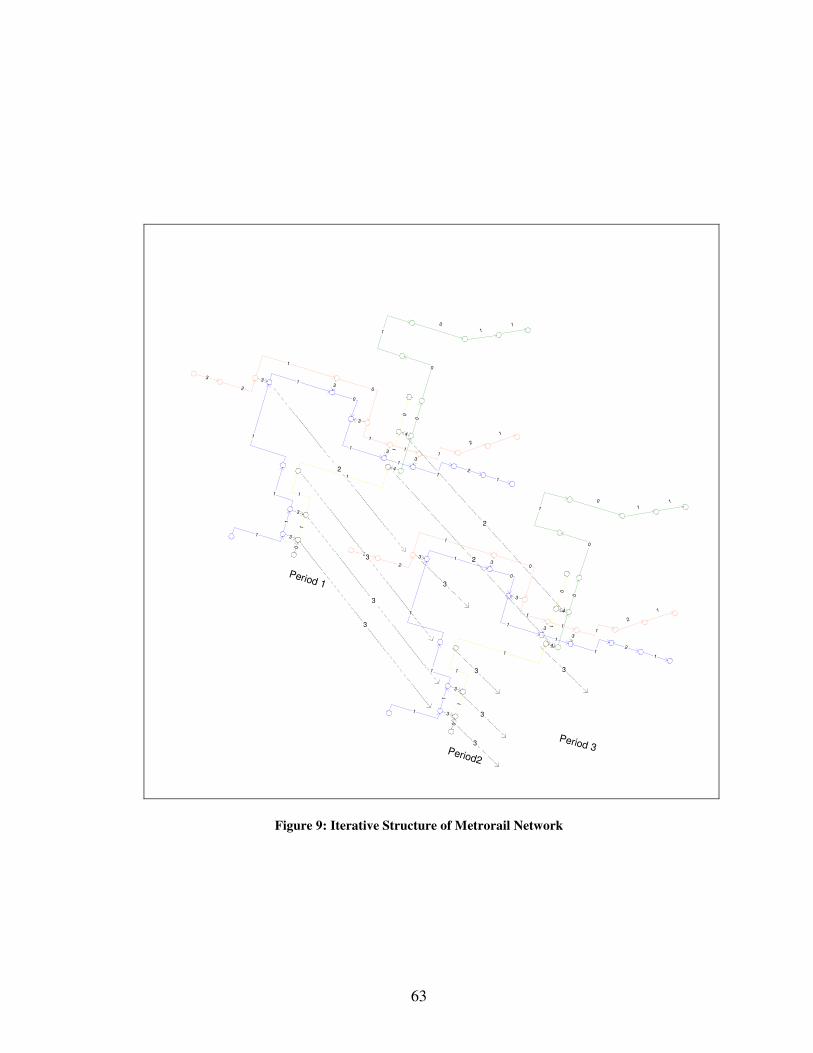
63

1

1

1

1

1

0

1

1

12

1

1

0

11

1

3

2

2

1

1

1

0

1

1

0

0

0

11

10

3

3

33

3

3

3

4

4

Period 1

1

1

1

1

1

0

1

1

12

1

1

0

11

1

3

2

2

1

1

1

0

1

1

0

0

0

11

10

3

3

33

3

3

3

4

4

Period2

3

3

3 2

2

2

3

3

3

3

Period 3

3

Figure 9: Iterative Structure of Metrorail Network

64

The train traffic network with slack times can be used to analyze the propagation of

delays in train networks. However, the magnitude of delay should not be so large as

to disrupt the planned order (in timetable) in which trains traverse shared track

sections. Long delays may invalidate the synchronization constraints too. Such

disruptions may alter the topology of the train-traffic network due to possible changes

in directionality of infrastructure and synchronization constraints. The delay

propagation algorithm assumes short delays that do not change the topology of the

train-traffic network. For large delays, a modified algorithm is presented later in

Chapter 4, which is used in the look-ahead method.

3.5 Delay Propagation Algorithm

Given the network, G = (N,A), with slack times, delay propagation of an initial set of

delays can be analyzed using the following algorithm:

Step1: Given initial set of delays at stations, create a “super-delay” node that

connects all the stations where delay occurs. The weights of the arcs that connect the

super-delay node to the stations would be the negative of delays that occur at those

stations.

Step2: Implement longest path algorithm to determine propagation of delays.

Longest Path Algorithm: This algorithm is a modified Dijkstra’s shortest path

algorithm. “Delay-updating” step and “permanent-labeling” steps are modified in this

algorithm.

65

Definitions:

N = Set of all nodes (including “super-delay” node)

A = Set of all arcs (including arcs connecting “super-delay” node to delayed stations)

sij = Slack on the arc connecting stations i, and j

S = Set of nodes with permanent “delay-labels”.

T = Set of nodes with temporary labels

d(i) = delay label at node i.

(i)+Γ = Set of outgoing arcs from node i.

3.5.1 Longest path algorithm

(1) Begin

(2) S: = {“super-delay” node}, T: = N - {“super-delay” node};

(3) d(i):= 0 ∀ i ∈ N;

(4) While S < N do begin

(5) let i ∈ T be a node for which d(i) = max{d(j): j ∈ T};

(6) S: = S U {i};

(7) T: = T – {i};

(8) for each j ∈ (i)+Γ do begin

(9) if d(j) < d(i) - sij then

(10) d(j): = d(i) - sij ;

(11) end;

(12) end;

(13) end;

66

The above algorithm gives the delay estimates at all the nodes in the network and

hence propagation of delay can be studied.

For the Metrorail network, the above algorithm was applied to determine the

propagation of delays for the initial delay set: 10 minutes delay at the beginning of

Blue and Orange lines (at stations Franconia-Springfield and Vienna/Fairfax

respectively). Longest path algorithm was applied to analyze the propagation of this

initial delay over the Metrorail network. Figure 10 shows the propagation of delays in

period 1. Thickness of a link represents the amount of delay experienced at the start

node of the link. Numbers on links represents the delay estimates, d(i), at the start

nodes of the links.

From the delay estimates, it can be observed that Blue, Orange and Yellow lines

experience delays in period 1. The delays spread to period 2 in case of Blue and

Orange lines. To characterize the propagation of delays, the following quantities are

defined and estimated:

• Number of stations reached: Number of stations at which trains are delayed due to

a given initial delay gives an estimate of spatial-propagation of delays in rail

network. This quantity is a measure of inter-connectedness of the rail network.

• Settling time: The time required for a given initial delay to get completely

absorbed or dissipated is termed as settling time. This quantity is a measure of

stability of the rail network.

67

For the Metrorail network, the initial delay of 10 minutes at two stations spreads to

fifteen other stations in the network. The settling time for the initial delay is forty

minutes.

10

8

7

6

5 4

4 3 2

1 0

5 4

32

4

10 7

1

0

5

4

0

3

22

5 2

Figure 10: Delay propagation in the first period

68

3.6 Stability Analysis

In this section, the study of variation in the amplitude of disturbance in train traffic

over space and time is of interest. The stability of train system can be defined as the

ability to recover to the original schedule after disruptions to the schedule. Recovery

to original schedule depends on the amount of slack present in timetable. As was

discussed previously, settling time (or recovery time) is a good measure of stability of

train timetable. The more the slack included in timetables, the faster the delays settle.

In the limiting case, if a timetable has no slack, delays will never settle. In this case,

timetable is considered unstable.

For the Metrorail network, the figures 11, 12 and 13 show the variation in the

amplitude of initial delay over space and time for Blue, Orange and Yellow lines (the

lines that are affected by the initial delay). From the figures, one can observe that for

Blue and Orange lines, the amplitude of delays decreases with time to zero (trains

recover to original schedule). However, both these lines experience knock-on delays

in the second period as shown in the figures 11 and 12. The amplitude of delays to

Yellow line reduces to a certain level and then remains constant as shown in figure 13.

The knock-on delay that the yellow line experiences does not settle (it does not

recover to original schedule) before it reaches its final destination. The Yellow line

has low stability due to limited slack in the running times.

69

0

1

2

3

4

5

6

7

8

9

10

Delay (minutes)

Franconia-Springfield

King Street ReaganAirport

Pentagon Rosslyn Farragut Metro Lenfant Capitol Armory Addison TownCenter

Stations

Delay to Blue line

Period 1

Period 2

Figure 11: Delay Amplitudes for the Blue Line

0

1

2

3

4

5

6

7

8

9

10

Delay (minutes)

Vienna Ballston Rosslyn Farragut Metro Lenfant Capitol Armory Cheverly New Carrolton

Stations

Delay to Orange line

Period 1

Period 2

Figure 12: Delay Amplitudes for the Orange Line

0

1

2

3

4

5

Delay (minutes)

Huntington ReaganAirport

L’Enfant ConventionCenter

Stations

Delay to Yellow line

Period1

Period 2

Figure 13: Delay Amplitudes for the Yellow Line

70

3.6.1 Critical Train

Critical train may be defined as a train with low stability and one that can cause large

number of knock-on delays in the network. A train with low stability is susceptible to

delays, and if such trains cause large knock-on delays, settling time or recovery time

of train traffic will increase. Delay propagation analysis of expected delays can be

used to determine critical train(s) in the network. Identifying critical train(s) would be

beneficial since improvements to stability of these trains would increase the stability

of the train network.

3.6 Summary and Conclusions

An analytical method for deterministic analysis of delay propagation and stability

analysis of train traffic networks was proposed in this chapter. The proposed method

is based on graph-theoretic concepts and is an alternate approach to the max-plus

algebraic method for deterministic stability analysis.

Project scheduling based approach was adopted to represent the

interdependencies between different rail services as a graph (network). For a given

timetable, the network was analyzed to determine the amount of slack time present in

running times and headway times. Timetables with no slack were termed as unstable

timetables as any disruption to trains running according to these timetables will never

settle. Timetables which have negative slack in at least one arc are termed as

unrealizable timetables as trains cannot operate according to these timetables without

requiring modifying schedules of some events. Hence, this method can be used to test

the feasibility or realizability of a timetable.

71

A longest path algorithm was proposed to analyze the propagation of an initial

set of delays over the rail traffic network. The delay estimates were used to

characterize the propagation of delays – number of stations affected by the delay, and

settling time of delay were defined as measures of interconnectedness of the rail

network and stability of timetable.

Stability of train network was defined as the ability of trains to recover to

original schedule after schedule disruptions. The variation of the amplitude of

disturbance to train traffic system over space and time characterizes the stability of

the system. In a stable train traffic system, the amplitude of disturbance reduces over

space and time and the system recovers eventually. In an unstable train traffic system,

on the other hand, the amplitude of disturbance remains the same and is not

dampened over space and time. Delay settling time was used as a measure of the

stability of train traffic system.

The proposed method was applied on real-life passenger rail network, the

Washington DC Metrorail network. In the delay propagation analysis, it was

assumed that the delays are not so large as to invalidate the timetable constraints. In

case of large delays, some of the infrastructure constraints may not be valid and thus

the delay propagation algorithm may not be applicable. Rescheduling strategies are

required to manage large disruptions in schedule, which are discussed in the next

chapter.

72

Chapter 4:

Modeling Uncertainty in Schedule Adherence: Large Delays

4.1 Introduction

Rail service reliability can be improved by implementing operational polices like

priority-based classification, train holding strategies, barrier reduction measures at

border stations, or infrastructure improvement policies. In order to evaluate different

operational policies, there is a need for a tool with the capability to make schedule

adjustments in response to large disruptions in original schedules. Large, unexpected

delays cause disruption in schedules and result in conflicting track access requests.

An operational simulation tool is presented in this chapter to manage conflicts and to

evaluate various operational policies aimed towards improving rail service reliability.

4.1.1 Conflict Management Policies

In practice, conflicts are resolved based on (local) priority of trains involved

in conflict. Passenger trains are given more priority over international freight trains,

which are given priority over regional freight trains. Another policy that is used in

practice specifies that the trains that follow their initial timetable have priority over

trains that are delayed (Tornquist, 2006). This policy may serve to isolate a disturbed

train and prevent the delay from spreading further. However, such policies may not

be beneficial in the long term. For example, a long-distance freight train may have

more slack in its schedule and can be delayed more than a short-distance freight train

operating on a tight schedule. Also, it may not be desirable to delay trains whose

73

schedules are synchronized with other trains in order to facilitate transfer of

shipments. Hence, it is important to consider secondary consequences of the

rescheduling decisions.

In some European countries, multiple carriers operate services that may share

the same infrastructure. Many carriers may compete for slots on shared track

segments. In such multi-carrier context, interests of all the stakeholders need to be

considered in making the rescheduling decisions. The objectives of rescheduling

decisions are thus context specific.

4.2 Related Works in Conflict Management

The challenge in conflict management is to resolve conflicts by considering the future

consequences of each decision in a stochastic dynamic environment. Unexpected

delays and network interdependencies make the prediction of future state of rail

traffic extremely difficult. Some works in the literature estimate the expected number

of conflicts and expected delay experienced by trains for single-line operations (for

example, Chen and Harker, 1990; Hallowell and Harker, 1998 ). These analytical

models estimate delay for a single rail line as opposed to a rail network and so

network interdependencies are not captured in these models.

The rescheduling problem is often formulated as a combinatorial optimization

problem, which is NP-complete for single track railway with a time complexity of

O(2n) for ‘n’ number of conflicts. Due to the size of the problem, dynamic nature and

limited time frame available to make rescheduling decisions, heuristic methods are

used to address the problem in the literature.

74

Kraft (1987) presents a branch-and-bound approach for resolving train

conflicts to minimize total delays. Higgins et al (1996 and 1997) formulate the

problem for a single-track line as a non-linear mixed integer program with an

objective to minimize train delay and fuel consumption. They propose a branch-and-

bound heuristic in the first paper and in the follow-up paper, they develop meta-

heuristic approaches. Tornquist (2006) presents a heuristic approach, HOAT, which

reevaluates the sequence of trains on segments for the delayed trains while

maintaining the initial sequence for the trains that are on schedule. This approach can

handle rescheduling on railway networks.

Sahin, Ahuja and Cunha (2004) formulate rescheduling as a multicommodity

flow problem in a space-time network. They propose integer programming based

heuristics that limit the maximum delay allowed to trains. They also propose a

simulation technique that solves each conflict based on a measure derived from LP-

relaxation of the problem. Their approach can handle rail networks but was tested on

a single-tracked rail line. A similar simulation-based technique was proposed by

Sahin (1999) for a single-tracked rail line. The method resolves conflicts locally in

the order they appear in time. One of the two trains in conflict is selected to stop

based on an approximate look-ahead heuristic measure, which is based on analytical

models that estimate expected delays.

Most of the techniques in the literature focus on a single objective of

minimizing total delay. However, delay to some trains may be more costly than delay

to others. For example, some trains may carry more valuable shipments or delaying

some trains may cause some shipments to miss their scheduled connections. As was

75

discussed in the previous section, objectives for rescheduling are often context

dependent, especially in a multi-carrier environment. Multiple carriers are considered

in market-based approaches to train scheduling, which use auction-based methods to

develop initial train timetables. Parkes and Ungar (2001) propose auction-based

method for the decentralized railway scheduling problem, where each train is

represented by a self-interested agent that bids for the right to travel across the

railway network from its origin to destination. However, there are only few works

that consider rescheduling strategies when multiple rail carriers compete for slots. For

example, Tornquist et al (2002) propose a multi-agent system approach to train delay

management problem. They identify train dispatchers and carriers as agents who

interact and negotiate, and whose decisions influence the propagation of delays in the

network. The use of agents was only applied as an abstraction modeling method and

the implementation was left as future work.

Also, many of the techniques in the literature assume single-line operations

and do not capture network effects. In this paper, we present a simulation tool to

evaluate different rescheduling policies in multi-carrier, rail networks.

4.3 Framework for Rescheduling in Multi-Carrier Rail Networks

Rescheduling is the process of updating an existing train schedule in response to

disruptions or other changes. Rescheduling in multi-carrier rail networks is discussed

in this section. The actors involved in rescheduling process are the dispatchers

associated with infrastructure managers, and the train service providers or carriers.

76

Train dispatcher is responsible to resolve conflicting slot requests, as was

discussed earlier. Besides priority-based resolution, the dispatcher may want to

consider other measures to resolve conflicts, which are discussed in detail later in the

section on conflict resolution.

Train carriers are independent actors that negotiate with the dispatcher for

access to slots with an aim to minimize disruptions to the trains they operate. When a

train gets delayed, it may lose the slots assigned according to the initial timetable. The

affected carrier will have to request new slots from the dispatcher. The carrier can

request new set of slots for all the remaining tracks in its path, but the train might get

delayed further due to conflicts with other trains or unexpected events and the new set

of slots may also be lost. In such a dynamic environment, the carrier may want to

negotiate for slots only for a few blocks ahead in its path in order to reduce the risk of

losing the slots after having obtained them. Hence, we propose a dynamic slot request

mechanism for the affected carriers.

4.3.1 Dynamic Slot Request Mechanism

Each affected carrier can request slots for N subsequent blocks ahead in its path. If

the request gets accepted, the slots are reserved for the train and are protected against

further disruptions. The train moves through the N tracks and upon completion, it

again requests slots for N subsequent blocks. As the trains request for slots

dynamically, the dispatcher can estimate the actual demand for slots better and this

helps the dispatcher make better slot allocation decisions. This method of dynamic

slot requests is similar in some respects to the method proposed by Lee and Ghosh

(1998) for dynamic planning of routes and schedules for point-to-point trains.

77

4.3.2 Trade-offs in Selecting the value of Slot Request Size (N)

From the carrier’s perspective, the value of N should not be so large as to

increase the risk of losing the slots due to unexpected events. A large N may also

increase the likelihood of the following undesirable situation: At the current time, the

delayed train (say Train A) may compete with Train B for a future time slot on block

L, and negotiate with the dispatcher to obtain the slot. However, Train B may later get

delayed before reaching block L and may use the block at a time that is not

conflicting with the slot requested by Train A. Such situations waste Train A’s effort

in negotiating for the slot when it was not necessary, and the likelihood of these

situations can be reduced by choosing smaller value of N. However, a large N may

also be beneficial to the delayed train since the reserved slots protect the train from

unforeseen disruptions and allow it to recover faster. Large value of N might also

allow the carrier to plan train velocity in order to minimize fuel consumption. In

summary, the value of N chosen by a carrier would depend on the level of uncertainty

in the rail network.

From the dispatcher’s perspective, large N is better in terms of safety since

signals and switches can be set appropriately to avoid collisions, deadlocks and so

forth. Large N also helps in giving the dispatcher a better estimate of the demand for

a particular slot and also more time to make better slot reallocation decisions.

However, reserving a large number of slots for a particular train may adversely affect

other critically delayed trains that may request for the same slots at a later time.

78

4.3.3 Slot Reservation

A slot reservation request consists of a list of N successive stations and the expected

arrival, departure times each of the stations. The expected arrival, departure times are

calculated based on the current time, the desired speed of the train, and lengths of the

blocks. Desired speed of the train is the maximum speed allowed by the infrastructure

or the speed allowed by the available locomotive power, whichever factor is

constraining. Traveling at the desired speed allows the train to utilize the slack in

running times in order to try and recover to the original schedule. In the calculation of

expected arrival, departure times, it is assumed that unexpected events do not occur at

the intermediate stations. For example, none of the intermediate stations should be a

border station, since the train loses its slots if it gets delayed again before utilizing all

the N slots. The arrival and departure times determine the (slot) time interval for

which a block reservation is desired.

The dispatcher evaluates the slot requests for each of the N blocks. The

dispatcher determines whether the requested slot for the first block is available. In

other words, the dispatcher detects if there are conflicting slot requests, which is

termed as conflict detection. If the slot is available, it is reserved. If, on the contrary,

the slot is already reserved for another train or is occupied at the current time, then

reservation cannot be made for the requested interval. Alternately, if the conflict is

such that the slot is not reserved for either train, the dispatcher resolves the conflict

based on some rules. This is termed as conflict resolution and is explained in detail in

the following section. If the reservation cannot be granted for the requested time

interval (say, t1 – t2), next earliest time interval is considered (beyond t2). The earliest

79

available slot (say, t3 – t4) is then reserved for the first block. The slot requests for the

subsequent blocks are modified to reflect the change in the interval reserved for the

first block. A similar reservation process is then initiated for the second block. This

process continues until slots are reserved for all N blocks. The delayed train continues

to request for reservation of N subsequent blocks until it reaches its destination. The

slot reservation process is shown in Figure 14.

T ra in d e la y e d ?

D e te c tC o n f lic t s

C o n flic t e x is ts ?

C o n flic tR e s o lu tio n

Y

S lo t a va ila b le ?

N

P re fe rr e d T im es lo t

U p d a teP re fe rre dT im e s lo t

N

Y

N

R e s e rv eS lo t

S to p

N b lo c k sre s e rv e d ?

Y

Y

Figure 14: Slot Reservation Process

80

4.3.4 Train Simulation

As discussed earlier, the proposed tool is embedded in a freight simulation platform

proposed in Mahmassani et al (2006). More specifically, the slot reservation

subroutine is called from the train moving part of the link moving subroutine in the

freight simulation platform. This is shown in the Figure 15.

In the link moving subroutine, whenever a train reaches a station, it is

determined whether the train departs from the station at the scheduled time. If the

train is delayed, slot reservation subroutine is called to reserve the next N blocks for

the delayed train. On the other hand, if the train is on schedule, it is not necessary that

the train can access the next slot without conflicting with other trains. This can be

ensured only when all the trains in the network are on schedule. Even if a single train

in the network is delayed, the original timetable cannot be considered conflict-free.

Hence, conflicts are detected even for trains that are on schedule.

For the train on schedule, the next track segment is checked for conflicts. If

the next slot is reserved for some other train, then the train needs to be delayed. Slot

reservation procedure is then called to reserve next N blocks for the train. Conversely,

if the slot is available, then it is reserved for the train. This procedure is shown in

Figure 16.

4.3.4 Conflict Detection

For a particular block (track-segment), the time slot requested by a train is compared

against the slots requested by other trains that share the block. If there is no conflict,

the slot is reserved for the train. If conflict exists, then conflict resolution procedure is

called. Conflict resolution procedure if described in the next section.

81

Figure 15: Train Simulation

82

Time slotreservation for next

N blocks

Train departing from stationon time?

Y

N

Conflict detectionfor the next block

Slot alreadyreserved?

N

Reserve the slot

Train arrived at station?

Y

Y

Figure 16: Conflict Detection embedded in Train Moving

4.3.5 Conflict Resolution

The measures that a dispatcher might consider in resolving conflicts are discussed in

this section. In practice, dispatchers use priority-based resolution methods. The type

of train (passenger trains, international freight train, regional freight train), value of

shipments carried by the train may determine the resolution decision. In case of

overtaking conflicts, train with higher speed is given priority over that with lower

speed. As was discussed earlier, priority based conflict resolution often tends to be

myopic as the secondary consequences of the decision are not accounted for.

83

4.3.5.1 Resolution Measures

When multiple carriers operate on the same infrastructure, the conflict resolution

strategies are dependent on the context of the conflict and the relationship between

the parties involved in the conflict. The following are some of the scenarios that may

occur:

Case 1: The dispatcher is a neutral agent, while two independent carriers compete for

the slot. In this case, both carriers negotiate with the dispatcher for the slot based on

their estimated cost of losing the slot. The more the estimated cost for a carrier, the

more competitive the carrier is expected to be. The slot is assumed to be awarded to

the carrier who is more competitive. The following are some of the measures the

carrier may use to estimate the cost of losing the slot:

Delay cost for train T at its destination, TDC :

An estimate of delay at the destination ( TD ) is obtained by an approximate look-

ahead procedure, which is explained in detail later. Value of time ( iVoT ) of the

shipments is used to estimate the total delay cost associated with delaying the train.

Value of time estimates are obtained from the mode-choice function used in the

freight simulation platform. If N is the number of shipments in the train, expected

delay cost is given by:

1

( ) *N

T i T

i

DC VoT D=

=� (18)

84

Shipment delay cost for train T, SDC :

It is to be noted that shipment delay is not the same as train delay. Some shipments in

a train may have missed their connections in previous legs of their journey and might

be critically delayed while other shipments in the same train may not be delayed.

From the estimated train delay at the destination, individual shipment delays ( iD ) can

be estimated. Total shipment delay cost is then calculated from the value of time of

shipments as shown below:

1

( ) *N

S i i

i

DC VoT D=

=� (19)

Number of shipments that miss their connection:

Arrival time of trains at intermediate loading, unloading points (shunting yard) is

estimated by the look-ahead procedure. Based on the expected departure time of the

connecting train from the shunting yard, the train holding policies, and the expected

processing time of shipments at the shunting yard, the number of shipments that

might miss their connections is estimated.

Case 2: The dispatcher is a neutral agent but the two trains involved in conflict are

operated by the same carrier. In this case, the conflict is resolved by the carrier and

not by the dispatcher. The carrier may use internal priority between trains to resolve

the conflict. The carrier may also use the measures described under Case 1.

85

Case 3: The same agent owns the infrastructure and operates the trains on the

network. In such cases, the objective of the dispatcher may be to minimize delay in

the network. The following are some of the measures the dispatcher may use in this

case:

Number of secondary delayed trains:

The look-ahead measure is used to estimate the number of secondary delays caused

by a delayed train. The train that causes lesser number of secondary delays is given

the slot.

Total delay cost to all the trains or all the shipments:

In addition to DCT (or DCS), delay cost due to all secondary delays are also estimated

in this measure. This measure reflects the network effects of delaying a train.

The measures described above can be estimated using a look-ahead procedure

described in the next section.

4.3.5.2 Look Ahead Method

The look-ahead method gives an approximate estimate of the future delay at the

destination of a train in conflict. It also gives an estimate of the secondary delays

caused due to the delayed train.

This method is based on train traffic network representation of the timetable,

discussed in Chapter 3. The delay propagation algorithm may not be applicable to

86

estimate future delays since large delays may invalidate infrastructure and

synchronization constraints. We propose a modified approach to estimate future

delays in this look-ahead method.

Estimated future delay to a particular train: Carrier perspective

The carrier of the delayed train (say, Train A) may want to run the train faster

in the future blocks by utilizing the slack in running times. The desired future time

slots may be in conflict with slots of other trains in the network. The potential

conflicts are predicted based on the slots requested by other trains on the shared

blocks according to their timetables. Priority-based resolution method is used to

resolve the potential conflicts. As each potential conflict is resolved, the desired

future time slots are updated and the process of detecting potential conflicts and

resolving them continues till Train A reaches its destination. Potential conflict

detection and resolution procedure is similar to the slot reservation procedure shown

in Figure 14. The estimated delay to Train A at its destination is the difference

between projected arrival time and the scheduled arrival time.

In resolving the potential conflicts for Train A, several other trains may have

been delayed. These secondary delays may cause further delays in the network. Some

dispatchers may be interested in the network effects of delaying Train A, in order to

resolve the current conflict. The following approach is proposed to estimate the

network effects of delaying a train.

87

Network effects of delay: System perspective

The method to estimate network effects of delaying a train is based on train

traffic network representation of the timetable, discussed previously. The topology of

the train traffic network is modified each time a train is delayed and the resulting

conflicts resolved. The latest network represents the current train traffic state at the

time of conflict involving Train A. The latest network topology is further modified to

reflect the changes in train orders due to projected conflict resolutions for Train A.

The propagation of the potential secondary delays is then analyzed on the modified

train traffic network using the delay propagation algorithm. It is assumed here that the

potential secondary delays do not change the topology of the train traffic network.

This method is an approximation but it gives a measure of the network wide impact

of delaying Train A in the current conflict.

The estimates of delay to Train A and the secondary delays caused by Train A can be

used in the measures described in Section 4.3.5.1.

4.4 Application: REORIENT Network

The proposed operational simulation tool was applied on a European rail freight

network, termed the REORIENT Network - which spans 11 countries of the

European Union, from Scandinavia to Greece. The EU has a vision for international

rail-based intermodal services that facilitate high-valued freight movement and is

sponsoring several research projects, like the REORIENT project, to examine the

market potential for such services. In the REORIENT project, four service options

88

were developed based on expert knowledge, in a trans-European North-South

corridor that originates in Scandinavia, cuts across Central Europe and is destined for

Southeastern Europe. The REORIENT corridor and the proposed services are shown

in Figure 17. The route details for the proposed services are given in Table 10. The

four services run through several international boundaries and the seamless

movement of freight on these services may be hindered by technological,

administrative barriers at the boundaries.

The delays at borders between nations are one of the critical deterrents to

seamless intermodal freight transport. These border-crossing delays can be reduced

by implementing some operational and administrative strategies like employing

compatible technologies (multi-voltage locomotives, uniform gauges and signaling

system), sending train manifests ahead of each train’s arrival, implementing

Information and Communication Technologies (ICT) for better communication,

developing standards to allow train drivers to operate internationally. Adopting these

policies may reduce the variability in border-delays and increase the service

reliability levels of the proposed services. To predict the impact of reducing

variability in border-delays, computational experiments were run in the proposed

operational simulation tool.

89

Figure 17: The REORIENT Corridor

Table 10: Route details for the proposed Services on REORIENT Corridor Route

identification Route design

T1

Halsberg-Trelleborg-Swinoujscie to via

Vienna/Bratislava to Budapest

T2 Trelleborg-via Swinoujscie to Bratislava/Vienna

T3 Gdansk/Gdynia-Bratislava/Vienna-Budapest-

Beograd- Thessalonica

T4 Bratislava –Budapest via Bucharest with Constantia

90

4.5 Design of Experiments

Computational experiments performed using the operational simulation tools are

described in this section. The experiments are designed primarily to test the impact of

varying degrees of delay times at border stations. The effect of including slack times

in timetable design, different rescheduling policies and different slot request sizes are

also examined using the proposed tool.

4.5.1 The Base Case: Scenario 1

The base case in these set of experiments corresponds to a scenario in the

REORIENT project where freight trains are scheduled all day along the four services

described previously. In this scenario, 52364 trains are scheduled over the

REORIENT network for a period of one week. Of the total number of trains, 572

trains are scheduled for the four services – T1, T2, T3 and T4. Streamlined border

operations are assumed and the mean border-delays are around 45 minutes to 1 hour.

It is also assumed in the base case that there is no variability in border delays. The

borders on the four services are shown in Figure 18. The Circles shown in the figure

indicate the border delay time assumed at a particular station. A smaller circle

indicates lower border crossing times. For example, at the Czech-Austrian border,

delay was assumed to be nearly 45 minutes, while delays at the Bulgaria-Greece

border were taken to be around an hour. The base case is referred to as Scenario 1.

91

Figure 18: Border Stations on the Reorient Corridor

4.5.2 Variability in Delays at Borders

Border delay scenarios are designed to test the effect of variability in border delays.

Three levels of variability in border delays are tested, which are described below:

Level 1: In level 1, border delays are assumed to vary uniformly between 15 minutes

to 2 hours (shown in Figure 19). The mean delay in this case is around 1 hour.

92

Figure 19: Uniform (15-120) Distribution to Model Border Delays Level 2: The variability in border delays is reduced in this level compared to level 1.

The border delays are assumed to vary uniformly between 30 to 90 minutes (shown in

Figure 20). The mean delay in this case is 1 hour.

Figure 20: Uniform Distribution (30-90) to Model Border Delays

Level 3: In this scenario, a triangular distribution (shown in Figure 21) is assumed

instead of uniform distribution as in Levels 1 and 2. The minimum and maximum

delays are assumed to be zero and 3 hours respectively, while the mode is assumed to

be 20 minutes. The mean delay in this scenario is also 1 hour.

93

Figure 21: Triangular Distribution to Model Border Delays

In testing the three border delay scenarios, the slack included in timetable design is

assumed to be the same. The slot request (or reservation) size, N, is also assumed to

be 5 for all three scenarios. It is also assumed in these experiments that each service is

operated by an independent carrier and so the rescheduling strategy adopted is from

the perspective of a carrier. The delay cost (as described under Case 1 in Section

4.3.5.1) to each of the trains in conflict is compared to resolve the conflicting track

access requests. These scenarios – Level 1, Level 2 and Level 3 variation in border

delays - are referred to as Scenarios 2, 3 and 4 respectively. This is shown in Table 11.

4.5.3 Slack Time in Timetable Design

Slack time is included in timetable design in headway times and running times to

absorb disruptions and help recover the train to original schedule, as discussed in

Chapter 3. However, increasing slack time in headways may result in lesser frequency

of service and increasing slack in running times results in slower trains, both of which

are not desirable to the shippers. To examine this trade-off, a timetable with more

94

slack in headways and running times is tested as Scenario 5. As a result of increasing

slack in headway times, the number of trains scheduled in a week for the four services

reduced from 572 to 378. Also the average speed of trains used in timetable design

reduced from 60 kmph to 40 kmph. The other parameters, variability in border delays

and slot request size (N) are fixed at Level 1 and five blocks respectively.

Rescheduling policy from the perspective of carrier is assumed in both the cases. The

effect of increasing slack in timetable design can be examined by comparing

Scenarios 5 and 2 since parameters other than slack are fixed at the same level. This

can be observed in Table 11.

4.5.4 Rescheduling Policy

As described earlier, rescheduling policy from the perspective of a carrier was

assumed in all the previous experiments. In this policy, each carrier tries to minimize

the disruption caused to the trains they operate. The network effects of delays are not

considered. Network effects are of interest in a scenario where the same agent is

responsible to resolve conflicts and operate the trains. Also, in a situation where the

carriers of the trains in conflict and those that may be affected due to secondary

delays cooperate and try to minimize the disruption to all the affected trains. The

secondary delays caused due to delaying a train in conflict can be estimated using the

look-ahead method described in section 4.3.5.2. Scenario 6 is designed to test the

effect of rescheduling policy from the system perspective by comparing it with

Scenario 2. As can be seen from Table 11, the other parameters are at the same level

for both the scenarios: border station delays are fixed at level 1, same amount of slack

is included in timetables, and slot request size is fixed at 5.

95

4.5.5 Slot Request Size (N)

The value of N chosen by a carrier would depend on the level of uncertainty in the

rail network, as was discussed in Section 4.3.2. A set of experiments are performed to

examine the effect of different values of N on total delay in the system. The different

values of N tested are 5, 15, 50 and 100 as Scenarios 2, 7, 8 and 9 respectively. Same

amount of slack is assumed to be included in the timetable for all these scenarios.

Variability in border delay is assumed to be at level 1 and rescheduling from the

perspective of carriers is assumed in all these scenarios. This can be observed in

Table 11.

An overview of all the scenarios 1 to 9 is shown in Table 11.

Table 11: Overview of Scenarios tested in Experiments

Variability in border delay Slack in timetables Rescheduling Policy Slot Request Size (N) S

CE

NA

RIO

S

None Level 1 U (15, 120)

Level 2 U (30, 90)

Level 3 T (0,180,20)

Less slack

More slack

Carrier Perspective

System Perspective 5 15 50 100

1 X X 2 X X X X 3 X X X X 4 X X X X 5 X X X X 6 X X X X 7 X X X X 8 X X X X 9 X X X X

96

4.6 Discussion of Results

The performance measures defined in Section 1.5 are used to compare the effect of

different scenarios. Some of the measures used are: service reliability, rail punctuality,

total delay, average delay, service desirability and rail mode share.

4.6.1 Effect of Variability in Border Delays

Three levels of variability in border times are tested as described in Section 4.5.2. The

mean and variance of the three levels of border delays are shown in Table 12.

Table 12: Mean and Variance of Border Delay Distributions Delay

Scenario Description Mean (min) Variance (min2) Level 1 U(15,120) 67 5512 Level 2 U(30,90) 60 1800 Level 3 T(0,180,20) 60 1622

As can be observed from Table 12, the mean of all the three levels is around 60

minutes but the variance in border delays drops from level 1 to 2 and from 2 to 3. The

decrease in border delay variability may reflect more streamlined border operations,

compatible technologies, and international agreements allowing personnel from one

country to run trains on another country’s network.

4.6.1.1 Effect of Variability in border delays on Total Delay in the System

The effect of decrease in variability in border crossing times on total delays in the

system is shown in Table 13 and Figure 22.

97

Table 13: Effect of Variability in Border Delays on Train Delays Delay

Scenario Total Delay

(min) Average Delay

(min) Level 1 1153067 80 Level 2 1151404 79.4 Level 3 1151097 79.3

1150000

1150500

1151000

1151500

1152000

1152500

1153000

1153500

Total Delay(min)

Level 1 Level 2 Level 3

Border delay scenarios

Effect of Variability in Border Delays

Figure 22: Effect of Variability in Border Delays on Total Delay in the System

From Figure 22, it can be observed that total delay in the system reduces as the

variability in border crossing times is reduced.

4.6.1.2 Effect of Variability in border delays on Service Reliability

The effect of reducing variability in border delays on service reliability levels is

examined for the four services. Table 14 and Figure 23 show the service reliability

levels on decreasing variability in border delays from Level 1 to Level 3.

98

Table 14: Service Reliability for Border-delay Levels 1 & 3 Service Reliability

Services Level 1 Level 3

T1 25% 30% T2 30% 35% T3 44% 47% T4 82% 87%

0

0.1

0.2

0.3

0.4

0.5

0.6

0.7

0.8

0.9

Reliability

T1 T2 T3 T4

Services

Service Reliabilty vs Delay

Level 1

Level 3

Figure 23: Effect of Reducing Variability from Level 1 to Level 3 on Service Reliability

Reducing the variability in border delays from Level 1 to Level 3 causes an increase

in the service reliability levels, as shown in Figure 23.

4.6.1.3 Effect of Variability in border delays on Service Desirability

The shipment ton-km attracted by a rail service is termed as service desirability.

Variability in border crossing times reduces the service desirability levels as shown in

Table 15 and Figure 24. Increase in service desirability may bring more revenue to

the carriers operating the service and hence reducing variability in border times is

also important from the perspective of carriers.

99

Table 15: Service Desirability vs. Variability in Border Delays

Service Desirability (Million Ton-Km)

Services No Variability Level 1 T1 35.9 33.6 T2 54.3 48.5 T3 210.5 194.8 T4 223.1 216.9

0

50

100

150

200

250

Ton-Km (million)

T1 T2 T3 T4

Services

Service Desirability vs. Variability in Border Delays

No Variability in DelayLevel 1

Figure 24: Comparing Service Desirability for Different Levels of Variability in Border Delays

4.6.2 Effect of Slack Time in Timetable Design

4.6.2.1 Effect of Slack Time on Average Delay in the System

Scenario 5 is tested by including more slack time in headway and running times in

timetable design. Including more slack time reduces the total delay and average delay

to the trains in the network. This is shown in Figure 25. This is as per expectation

since slack time limits the propagation of delays in the network. Hence, including

more slack in the timetables makes the train network more stable.

100

80

74

71727374757677787980

Less Slack More Slack

Slack Time in Timetable vs Average Delay

Average Delay (minutes)

Figure 25: The effect of Slack Time on Average Delay in the System

4.6.2.2 Effect of Slack Time on Rail Punctuality and Service Reliability

The percentage of trains in the network that reach their destination at the scheduled

time is termed as rail punctuality. As the amount of slack is increased, rail punctuality

also increases as shown in Figure 26.

83%

85%

82%

83%

83%

84%

84%

85%

85%

Less Slack More Slack

Rail Punctuality

Figure 26: Rail Punctuality vs. Slack Time in Timetable

Including more slack in the timetables also increases service reliability of rail services,

in general. This is shown in Table 16 and Figure 27.

101

Table 16: Slack in Timetable vs. Service Reliability

Service Reliability Services Less Slack More Slack

T1 25% 90% T2 30% 50% T3 44% 78% T4 82% 67%

0

0.1

0.2

0.3

0.4

0.5

0.6

0.7

0.8

0.9

Reliability

T1 T2 T3 T4

Services

Service Reliability versus Slack

Less Slack

More Slack

Figure 27: The effect of Slack Time on Service Reliability

Hence, increasing slack time in timetable design has the positive effects of reducing

average delay in the network, increasing rail punctuality and service reliability.

However, increasing slack also results in lower frequency of service and slower trains.

In this scenario, including more slack in timetable caused the number of scheduled

trains for the four services to drop from 572 to 378 as shown in Figure 28.

102

572

378

0

100

200

300

400

500

600

Number of Trains

Less Slack More slack

Slack in Timetable

Number of Scheduled Trains vs Slack

Figure 28: The effect of Slack time on the number of scheduled trains in the system

Scheduling lesser number of trains in the system may decrease the capacity utilization

and thus may reduce the profit margins for the infrastructure manager. From the

perspective of a shipper, lesser service frequency and slower trains may make the rail

service less attractive.

4.6.2.3 Effect of Slack Time: Trade-off between Stability of train network and

Frequency of Service offered.

As was discussed earlier, including more slack in timetable design reduces total delay

in the system, which is a measure of the stability of train traffic network. However,

increasing slack in headways also leads to lesser frequency of service offered to the

shippers. To examine the trade-off between stability of train network and frequency

of service offered, the shipment ton-km attracted by the four services is examined.

103

493

499

491

492

493

494

495

496

497

498

499

500

Million Ton-Km

Less Slack More Slack

Total Shipment Ton-Km Attracted by Four Services

Figure 29: The Effect of Slack time on Shipment Ton-Km Attracted by Four Services As the amount of slack included in timetable is increased, the shipment ton-km

attracted by the four services also increases. In the trade-off between train delays and

service frequency, train delays seem to dominate. This can also be demonstrated at

the individual service level. From Table 17 and Figure 30, it can be observed that

each of the four services attracts more shipment ton-km when more slack is

introduced in the timetable.

Table 17: Service Desirability vs. Slack Time

Service Desirability (Million Ton-Km)

Services Less Slack More Slack T1 33.6 34.6 T2 48.5 51.2 T3 194.8 196.6 T4 216.9 217.1

104

0

50

100

150

200

250

Million Ton-Km

T1 T2 T3 T4

Services

The effect of Slack time on Service Desirability

Less Slack

More Slack

Figure 30: Service Desirability vs. Slack Time

4.6.3 Effect of Rescheduling Policy

The effects of rescheduling policy from the perspective of a carrier and from the

perspective of the system were tested in the platform. When the rescheduling policy is

based on each carrier trying to minimize disruptions to the trains they operate, the

average delay to trains in the system is noted to be 80 minutes. When the network

effects of delay a train are considered in managing conflicts, the average delay to the

trains in the system reduced to 67 minutes. Therefore, when the rescheduling policy is

based on minimizing delay to all the trains in the system, irrespective of carriers

operating them, average delay to trains in the system reduces by 16%. This can be

observed in Figure 31.

105

80

67

60

62

64

66

68

70

72

74

76

78

80

Average Delay (min)

Carrier Perspective System Perspective

Effect of Rescheduling Policy

Figure 31: Effect of Rescheduling Policy on Average Delay to Trains in the System

4.6.4 Effect of Slot Request Size (N)

Effect of varying the value of slot request size (N) is examined for four different

values of N in Scenarios 2, 7, 8 and 9. As the value of N is increased, the average

delay to trains in the system decreases. This can be observed in Table 18 and Figure

32. Rail punctuality, however, remains the same (83%) in all the four scenarios.

The following reason may explain the reduction in average delays as the value

of N is increased: The only source of randomness in the network in these set of

experiments is the variability in border delays. There are only around ten borders and

these borders are located far apart from each other as can be in Figure 18. Since there

is limited uncertainty in the system, carriers may want to choose large value of N to

reserve large number of slots for the trains operated by them. Reserving large number

of slots protects the trains from unforeseen disruptions (secondary delays) and allows

them to recover faster. Large value of N can thus result in lower delays in the network.

106

Table 18: Average Delay to Train for Different Values of N

N Average Delay

(min) 5 80 15 78 50 78 100 77

75

75.5

76

76.5

77

77.5

78

78.5

79

79.5

80

Average Delay (min)

N=5 N=15 N=50 N=100

Slot Request Size (N)

Average Delay Vs. Slot Request Size

Figure 32: The effect of Slot Request Size on Average Delay in the System

4.6 Summary and Conclusions

Operational simulation tool was presented in this chapter to model uncertainties and

apply rescheduling strategies in case of schedule disruptions due to unforeseen events.

Rescheduling strategies in multi-carrier environment were discussed. A dynamic slot

request mechanism was proposed to model the slot request behavior of carriers in a

dynamic, stochastic environment. Carrier of a delayed train may want to request slots

only for N blocks ahead in its path in order to minimize the risk of losing the slots. In

this approach, it was assumed that the dispatcher allocates the slot to the more

competitive carrier. The carriers compete for the slot based on the estimated cost of

losing the slot. A look-ahead method was proposed to estimate the delay cost at the

destination of a train if it loses the slot in the current conflict. The proposed look-

107

ahead method can also predict secondary delays caused due to delaying a particular

train based on delay propagation algorithm.

The proposed operational simulation tool was applied on REORIENT network.

Scenarios were designed to assess the effect of variability in border crossing times,

slack times in timetable, different rescheduling policies and the slot request size (N).

Different levels of variability in border crossing times were tested using the

tool. As the variability in border delays was reduced, it was found that average delay

to trains in the network decreased and service reliability increased. It was also found

that the service desirability levels increased on decreasing the level of variability in

border delays. These effects were according to prior expectation. The main

contribution of the proposed approach was to quantify the benefits of reducing

variability in border delays.

The effect of increasing slack time in headways and running times was

examined using the tool. It was found that on increasing the slack in timetable, the

average delay to trains in the network decreases and service reliability levels increase.

However, increasing slack also resulted in decreased service frequency and slower

trains, both of which are not desirable to the shippers. The shipment ton-km attracted

by the services were compared before and after increasing the amount of slack time in

timetable to examine the trade-off between average delay in the network and level of

service offered to the shippers. It was found that the services attracted more shipment

ton-km on increasing the amount of slack time suggesting that trains delays are more

important than the frequency of service offered in the test scenario.

108

Two different rescheduling policies were tested in the tool, namely

rescheduling from the carrier perspective and that from the system perspective. It was

found that rescheduling from the system perspective results in 16% reduction in

average delay to the trains in the system. This indicates the importance of considering

secondary effects of delaying trains when resolving conflicts.

Another set of experiments tested the effect of different values of slot request

size (N). It was found that as the value of N increased, average delay to trains in the

system reduced, while rail punctuality remained the same. This may be due to limited

number of border crossings in the network and the fact that variability in border

delays were the primary source of uncertainty in the scenarios that were tested. When

the level of uncertainty in the network is low, the carriers may want to request for

reserving large number of blocks ahead in the path of their trains in order to protect

them from secondary disruptions and allow them to recover faster.

109

Chapter 5:

Conclusions

5.1 Introduction

This thesis presents an operational simulation tool to evaluate different rail

operational policies aimed toward increasing service reliability in large-scale multi-

carrier rail networks. Service reliability is one of the most important factors that

shippers consider in choosing mode to transport freight. Train schedule reliability and

shipment connection reliability are service reliability measures of interest to train

carriers and shippers respectively. Operational policies that can improve these

measures of reliability were discussed in this thesis.

5.2 Summary and Contributions

Shipment connection reliability can be improved by adopting policies such as

priority-based classification, train holding and train cancellation strategies. The

application of the bulk queueing model proposed in Mahmassani et al (2006) to

support the evaluation of these operational policies was described. In order to

implement priority-based classification, the additional operational decisions that need

to be made were discussed. An optimization based framework was proposed to

implement priority based classification. Hump sequencing problem and dynamic

block to track assignment problem are the components of the framework. To

determine an optimal hump sequence, the hump sequencing algorithm proposed by

Kraft (2000 b) was adopted. The dynamic block to track assignment problem was

110

proposed to be solved in two sequential steps. Integer programming formulations

were proposed for each step and were demonstrated on a small example problem. The

framework can be used to identify jeopardized connections much sooner. This

method can protect the connections of high priority cars by “rehumping” low priority

cars and eliminates the need for an inefficient “cherry-picking” procedure to dig high

priority cars from among other rail cars before train assembly process. Implementing

priority based classification to protect the connections of high priority cars can

improve service reliability and service desirability.

Train schedule reliability is dependent on the propagation of delays in train

networks. An analytical method for deterministic analysis of propagation of minor

delays in train traffic networks was proposed. The proposed method is based on

graph-theoretic concepts, where the interdependencies between different rail services

are represented as a graph (network). For a given timetable, the network was analyzed

to determine the amount of slack time present in running times and headway times.

Timetables with no slack were termed as unstable timetables as any disruption to

trains running according to these timetables will never settle. A longest path

algorithm was proposed to analyze the propagation of an initial set of delays over the

rail traffic network. The delay estimates, like the number of stations affected by the

delay, and settling time of delay were used to characterize the propagation of delays,

and the stability of train networks. Stability of train networks was defined as the

ability of trains to recover to original schedule after schedule disruptions. The

variation of the amplitude of disturbance to train traffic system over space and time

characterizes the stability of the system. In a stable train traffic system, the amplitude

111

of disturbance reduces over space and time and the system recovers eventually. Delay

settling time was used as a measure of the stability of train traffic system. The

proposed method was applied on the Washington DC Metrorail network. In the delay

propagation analysis, it was assumed that the delays are not so large as to invalidate

the timetable constraints. In case of large delays, some of the infrastructure

constraints may not be valid and thus the delay propagation algorithm may not be

applicable. Rescheduling strategies are required to manage large disruptions in

schedule.

In order to manage large disruptions in schedule, an operational simulation tool was

proposed to apply rescheduling strategies. Strategies to reschedule in multi-carrier

environment were discussed. A dynamic slot request mechanism was proposed to

model the slot request behavior of carriers in a dynamic, stochastic environment. In

order to minimize the risk of losing the slots, carrier of a delayed train may want to

request slots only for N blocks ahead in the path of the trains they operate. In this

approach, it is assumed that the dispatcher allocates the slot to the more competitive

carrier. The carriers compete for the slot based on the estimated cost of losing the slot.

A look-ahead method was proposed to estimate the delay cost at the destination of a

train if it loses the slot in the current conflict. The proposed look-ahead method can

also predict secondary delays caused due to delaying a particular train based on delay

propagation algorithm. The secondary effects of delaying a train are of interest where

the same agent is responsible for resolving conflict and operating train services. The

proposed operational simulation tool was applied on REORIENT network. Scenarios

were designed to assess the effect of variability in border crossing times, slack times

112

in timetable, and the slot request size (N). As the variability in border crossing times

was reduced, average delay to the trains in the network reduced. It was also found

that it led to increase in service reliability and service desirability as expected. The

effect of increasing slack time in headways and running times was also examined

using the tool. It was found that on increasing the slack in timetable, the average

delay to trains in the network decreases and service reliability increases. However,

increasing slack also resulted in decreased service frequency and slower trains, both

of which are not desirable to the shippers. The trade-off between train delays and

service quality was examined by comparing the shipment ton-km attracted by the

services. It was found that the services attract more shipment ton-km on increasing

slack time in the timetable, suggesting that reduced train delay dominates the effect of

decreased level of service. Two rescheduling policies were also tested in the tool,

namely rescheduling from carrier perspective and rescheduling from the system

perspective. It was found that rescheduling from the system perspective resulted in

16% reduction in average delay to the trains in the system. Another set of

experiments tested the effect of different values of slot request size (N). It was found

that as the value of N increased, average delay to trains in the system reduced, while

rail punctuality remained the same.

Thus, the ability of the simulation tool to test operational policies such as

those to reduce barriers at border crossings, and to examine trade-off between

stability and capacity utilization in large-scale multi-carrier rail networks has been

demonstrated. It was also shown that the tool can predict the impact of adopting

various policies on service reliability and service desirability, which are of interest to

113

rail carriers and reflect shipper behavior. The tool can also test the policies to improve

shipment connection reliability (priority-based classification, train holding and

cancellation policies). The method to implement these policies was described but was

not demonstrated on a network.

5.3 Limitations and Directions for Future Research

The tool assumes conflicts to occur only due to line blocking constraints. However,

other practical constraints like station capacity, arrival and departure headways at

stations can also cause conflicts. These constraints were not considered in the

proposed tool. Also, the tool assumes fixed blocking safety system that allows only

one train per track segment. In new safety systems, like European Rail Traffic

Management System (ERTMS), resources are dynamically allocated according to

speeds of trains, acceleration rates, deceleration rates, reaction times of drivers among

other factors. Such safety systems are not modeled in the operational simulation tool.

The conflict resolution procedure used in the tool is based on an approximate

look-ahead method that estimates the cost of losing a slot for a carrier involved in

conflict. This method can be improved in the future by using optimization based

approaches that can capture the network effects of delaying a train more accurately.

114

Appendices

115

116

Bibliography

Adenso-Diaz, B., Olivia González, M., and González-Torre, P. (1999), “On-line

timetable re-scheduling in regional train services,” Transportation Research Part B,

Vol 33, P 387– 398.

Ahuja, R. K., Magnanti, T. L., and Orlin, J. B. (1993). Network Flows – Theory,

Algorithms, and Applications. Prentice Hall.

Carey and Malachy, (1999) “Ex ante heuristic measures of schedule reliability”,

Transportation Research Part B ,Vol 33(7), P 473-494.

Carey, M and Lockwood, J, (1995) “A Model, Algorithms and Strategy for Train

Pathing”, Journal of the Operational Research Society Vol 46, P 988-1005.

Carey, M., Lockwood, D. (1995), “A model, algorithms and strategy for train

pathing”, Journal of the Operational Research Society Vol 46. P 998-1005.

Chen, B. and Harker, P.T. (1990), “Two moments estimation of the delay on single-

track rail lines with scheduled traffic”, Transportation Science, P 261-275.

Cordeau, J-F., Toth, P., Vigo, D. (1998), “A survey of optimization models for train

routing and scheduling” Transportation Science, Vol. 32 (4), P 380-404.

Crainic T.G, Florian M, and Leal J.E (1990), "A Model for the Strategic Planning of

National Freight Transportation by Rail," Transportation Science, Vol. 24, P 1-24.

Crainic T.G. (1998), “A survey of optimization models for long-haul freight

transportation”, Publication CRT-98-67, Centre de recherche sur les transports,

Université de Montréal., Canada.

117

D. C. Parkes and L. H. Ungar, (2001), “An auction-based method for decentralized

train scheduling”, In Proceedings of AGENTS’01, Montreal, Quebec, Canada, May

2001, ACM.

Daganzo, C. F. (1986), “Static Blocking at Railyards: Sorting Implications and Track

Requirements”, Transportation Science. Vol. 20, P 189-199.

Daganzo, C. F., Dowling, R. G. and Hall, R. W. (1983), “Railroad Classification Yard

Throughput: The Case of Multistage Triangular Sorting” Transportation Research A,

Vol 17, P 95-106

EUROSTAT. (2007), “Road share of inland freight transport”, Available online:

http://ec.europa.eu/eurostat.

Fernandez, J.E, Joaquin De Cea, Ricardo Giesen, E. (2004), “A Strategic Model of

Freight Operations for Rail Transportation Systems”. Transportation Planning and

Technology Vol. 27, P 231-260.

Goverde and Odijk, (2002) “Performance evaluation of network timetables using

PETER”, Computers in Railways VIII, WIT Press.

Goverde, R.M.P (2005), Punctuality of Railway Operations and Timetable Stability

Analysis, PhD thesis, Delft University of Technology.

Hallowell, S., Harker. P. (1998), “Predicting on-time performance in scheduled

railroad operations: Methodology and application to train scheduling”,

Transportation Research Part A, Vol. 32(4), P 279-296.

Hallowell, S.F. and P.T. Harker (1998) “Predicting on-time performance in scheduled

railroad operations: methodology and application to train scheduling”, Transportation

Research A, Vol 32(6), P 279–295.

118

Higgins, A. and E. Kozan (1998) “Modeling train delays in urban networks”,

Transportation Science, Vol 32(4), P 346–357.

Iyer, R.V., Gosh, S. (1995), “DARYN – A distributed decision-making algorithm for

railway networks: Modeling and Simulation”, IEEE Transactions on Vehicular

Technology, Vol. 44 (1), P 180-191.

Jean-François Cordeau, Paolo Toth, and Daniele Vigo. (1998), “A survey of

optimization models for train routing and scheduling”. Transportation Science, Vol.

32, P 380-404.

Kraay, D., Harker, P. (1995), “Real-time scheduling of freight railroads”

Transportation Research Part B, Vol. 29B (3) P 213-229.

Kraft, E. R. (2000), “A Hump Sequencing Algorithm for Real Time Management of

Train Connection Reliability”, Journal of the Transportation Research Forum Vol 39,

P 95-115, published jointly with Transportation Quarterly, Fall 2000 edition, Vol 54.

Kraft, E. R. (2000), “Implementation Strategies for Railroad Dynamic Freight Car

Scheduling”, Journal of the Transportation Research Forum Vol. 39, P 119-137,

published jointly with Transportation Quarterly, Summer 2000 edition, Vol. 54.

Kraft, E. R. (2002) “Priority-Based Classification for Improving Connection

Reliability in Railroad Yards -- Part II: Dynamic Block to Track Assignment”,

Journal of the Transportation Research Forum Vol. 56, P 107-119.

Kraft, E. R. (2002), “Priority-Based Classification for Improving Connection

Reliability in Railroad Yards -- Part I: Integration with Car Scheduling”, Journal of

the Transportation Research Forum, Vol. 56, P 93-105.

119

Kraft, E., (1987), “A branch and bound procedure for optimal train dispatching”,

Journal of the Transportation Research Forum, Vol 28, P 263– 276.

Mahmassani, H. S., K. Zhang, J. Dong, C.-C. Lu, V. C. Arcot, and E. Miller-Hooks,

(2007), “A dynamic network simulation-assignment platform for multi-product

intermodal freight transportation analysis” Accepted for publication in Transportation

Research Record, Journal of TRB.

Martland C.D (1982), “PMAKE Analysis: Predicting Rail Yard Time Distributions

Using Probabilistic Train Connection Standards,” Transportation Science, Vol. 16, P

476-506.

Middelkoop, D. & Bouwman, M., (2000) “Train Network Simulator for Support of

Network Wide Planning of Infrastructure and Timetables”. Computers in Railways

VII, WIT Press: Southampton, P 267-276.

Nordeen, M., (1996) Stability Analysis of Cyclic Timetables for a Highly

Interconnected Rail Network, PhD Thesis, EPFL, Lausanne.

Patty, B., (2001) “The Use of Optimization to Improve Freight Railroad Service

Reliability”, Presented at IMA Workshop on Optimization in Travel and

Transportation.

Petersen E.R (1977), "Railyard Modelling: Part I. Prediction of Putt-through Time,"

Transportation Science, Vol. 11, P 37-49.

Petersen E.R (1977), "Railyard Modelling: Part II. The Effect of Yard Facilities on

Congestion”, Transportation Science, Vol. 11, P 50-59.

Petersen, E., Taylor, A. (1982), “A structured model for rail line simulation and

optimization”, Transportation Science, Vol. 16 (2), P 192-206.

120

Petersen, E.R. (1974), “Over-the-road transit time for a single track railway”,

Transportation Science , Vol 8(1), P 65-74.

Powell, W. B. (1986b), “Iterative Algorithms for Bulk Arrival, Bulk Service Queues

with Poisson and Non Poisson Arrivals”, Transportation Science, Vol 20.

Reebie Associates, (1972) “Toward an effective demurrage system”, US Department

of Transportation. Federal Railroad Administrator.

�ahin, G., Ahuja, R.K., Cunha, C.B. (2005). “New approaches for the train

dispatching problem”, submitted to Transportation Research Part B.

�ahin, �. (1999), “Railway traffic control and train scheduling based on inter-train

conflict management”, Transportation Research Part B, Vol. 33, P 511-534.

Simao, H. P. and W. B. Powell, (1992) “Numerical Methods for Simulating Transient,

Stochastic Queueing Networks—I: Methodology”, Transportation Science Vol 26, P

296-311.

Simao, H. P. and W. B. Powell, (1992) “Numerical Methods for Simulating Transient,

Stochastic Queueing Networks-II: Experimental Design”, Transportation Science Vol

26, P 312-329.

Törnquist, J. and Davidsson, P. (2002). “A Multi-Agent System Approach to Train

Delay Handling”, Proceedings from Agent Technologies in Logistics workshop, The

15th European Conference on Artificial Intelligence, Lyon, France.

121

Tornquist, J., (2006), “Computer-based decision support for railway traffic

scheduling and dispatching: a review of models and algorithms”, Presented at

ATMOS 2005, Palma de Mallorca, Spain, October 2005.

Turnquist M.A, Daskin M.S (1982), “Queuing Models of Classification and

Connection Delay in Railyards,” Transportation Science, Vol. 16, P 207-230.

Yagar, S. and Saccomanno, F. F. (1983), “An Efficient Sequencing Model for

Humping in a Rail Yard”, Transportation Research A, Vol 17, P 251-262