Viscosity Solutions for Dummies(including Economists)

Online Appendix to

“Income and Wealth Distribution in Macroeconomics:A Continuous-Time Approach”

written by Benjamin Moll

August 13, 20171

Viscosity Solutions

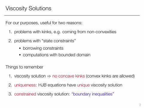
For our purposes, useful for two reasons:

1. problems with kinks, e.g. coming from non-convexities

2. problems with “state constraints”• borrowing constraints• computations with bounded domain

Things to remember

1. viscosity solution⇒ no concave kinks (convex kinks are allowed)

2. uniqueness: HJB equations have unique viscosity solution

3. constrained viscosity solution: “boundary inequalities”

2

References

Relatively accessible ones:• Lions (1983) “Hamilton-Jacobi-Bellman Equations and the Optimal

Control of Stochastic Systems” – report of some results, no proofshttp://www.mathunion.org/ICM/ICM1983.2/Main/icm1983.2.1403.1418.ocr.pdf

• Crandall (1995) “Viscosity Solutions: A Primer”http://www.princeton.edu/~moll/crandall-primer.pdf

• Bressan (2011) “Viscosity Solutions of Hamilton-Jacobi Equationsand Optimal Control Problems”https://www.math.psu.edu/bressan/PSPDF/hj.pdf

• Yu (2011) http://www.math.ualberta.ca/~xinweiyu/527.1.08f/lec11.pdf

Less accessible but often cited:• Crandall, Ishii and Lions (1992) “User’s Guide to Viscosity Solutions”• Bardi and Capuzzo-Dolcetta (2008)

https://www.dropbox.com/s/hsihfm8xwnnncvy/bardi-capuzzo-wholebook.pdf?dl=0

• Fleming & Soner (2006)https://www.dropbox.com/s/wbekmg2icp5u9i1/fleming-soner-wholebook.pdf?dl=0

3

Outline

1. Definition of viscosity solution

2. No concave kinks

3. Constrained viscosity solutions

4. Uniqueness

4

Viscosity Solutions: Definition

Consider HJB for generic optimal control problem

ρv(x) = maxα∈A

{r(x, α) + v ′(x)f (x, α)

}(HJB)

• Next slide: definition of viscosity solution• Basic idea: v may have kinks i.e. may not be differentiable• replace v ′(x) at point where it does not exist (because of kink in v )

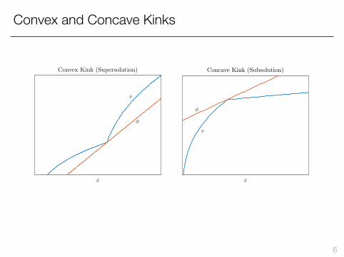
with derivative of smooth function ϕ touching v• two types of kinks: concave and convex⇒ two conditions

• concave kink: ϕ touches v from above• convex kink: ϕ touches v from below

• Remark: definition allows for concave kinks. In a few slides: thesenever arise in maximization problems

5

Convex and Concave Kinks

x

v

φ

Convex Kink (Supersolution)

x

v

φ

Concave Kink (Subsolution)

6

Viscosity Solutions: Definition

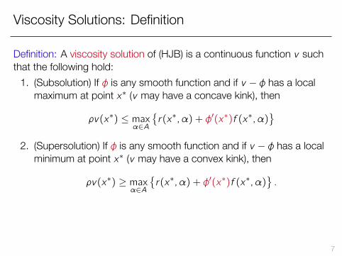
Definition: A viscosity solution of (HJB) is a continuous function v suchthat the following hold:

1. (Subsolution) If ϕ is any smooth function and if v − ϕ has a localmaximum at point x∗ (v may have a concave kink), then

ρv(x∗) ≤ maxα∈A

{r(x∗, α) + ϕ′(x∗)f (x∗, α)

}2. (Supersolution) If ϕ is any smooth function and if v − ϕ has a local

minimum at point x∗ (v may have a convex kink), then

ρv(x∗) ≥ maxα∈A

{r(x∗, α) + ϕ′(x∗)f (x∗, α)

}.

7

A few remarks, terminology

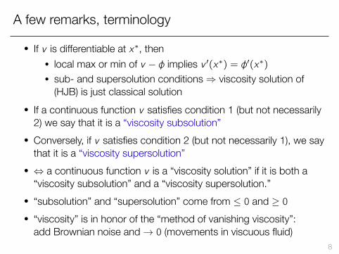
• If v is differentiable at x∗, then• local max or min of v − ϕ implies v ′(x∗) = ϕ′(x∗)• sub- and supersolution conditions⇒ viscosity solution of

(HJB) is just classical solution• If a continuous function v satisfies condition 1 (but not necessarily

2) we say that it is a “viscosity subsolution”• Conversely, if v satisfies condition 2 (but not necessarily 1), we say

that it is a “viscosity supersolution”• ⇔ a continuous function v is a “viscosity solution” if it is both a

“viscosity subsolution” and a “viscosity supersolution.”• “subsolution” and “supersolution” come from ≤ 0 and ≥ 0• “viscosity” is in honor of the “method of vanishing viscosity”:

add Brownian noise and→ 0 (movements in viscuous fluid)8

Viscosity Solutions: Intuition

• Consider discrete time Bellman:

v(x) = maxαr(x, α) + βv(x ′), x ′ = f (x, α)

• Think about it as an operator T on function v

(Tv)(x) = maxαr(x, α) + βv(f (x, α))

• Solution = fixed point: Tv = v• Intuitive property of T (“monotonicity”)

ϕ(x) ≤ v(x) ∀x ⇒ (Tϕ)(x) ≤ (Tv)(x) ∀x (∗)• Intuition: if my continuation value is higher, I’m better off

• Viscosity solution is exactly same idea• Key idea: sidestep non-differentiability of v by using “monotonicity”

9

Viscosity Solutions: Heuristic Derivation

• Time periods of length ∆. Consider HJB equationv(xt) = max

α∆r(xt , α) + (1− ρ∆)v(xt+∆) s.t.

xt+∆ = ∆f (xt , α) + xt

• Suppose v is not differentiable at x∗ and has a convex kink• problem: when taking ∆→ 0, pick up derivative v ′

• solution: replace continuation value with smooth function ϕ

x

v

φ

Convex Kink (Supersolution)

10

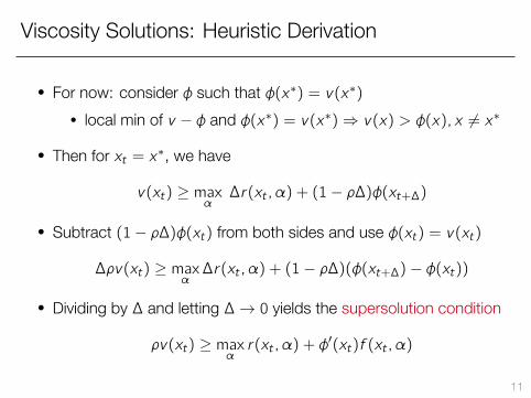
Viscosity Solutions: Heuristic Derivation

• For now: consider ϕ such that ϕ(x∗) = v(x∗)• local min of v − ϕ and ϕ(x∗) = v(x∗)⇒ v(x) > ϕ(x), x = x∗

• Then for xt = x∗, we have

v(xt) ≥ maxα∆r(xt , α) + (1− ρ∆)ϕ(xt+∆)

• Subtract (1− ρ∆)ϕ(xt) from both sides and use ϕ(xt) = v(xt)

∆ρv(xt) ≥ maxα∆r(xt , α) + (1− ρ∆)(ϕ(xt+∆)− ϕ(xt))

• Dividing by ∆ and letting ∆→ 0 yields the supersolution condition

ρv(xt) ≥ maxαr(xt , α) + ϕ

′(xt)f (xt , α)

11

Viscosity Solutions: Heuristic Derivation

• Turns out this works for any ϕ such that v − ϕ has local min at x∗

• define κ = v(x∗)− ϕ(x∗). Then v(x∗) = ϕ(x∗) + κ and

v(xt) ≥ maxα∆r(xt , αt) + (1− ρ∆)(ϕ(xt+∆) + κ)

• subtract (1− ρ∆)(ϕ(xt) + κ) from both sides

∆ρv(xt) ≥ maxα∆r(xt , α) + (1− ρ∆)(ϕ(xt+∆)− ϕ(xt))

• rest is the same...

• Derivation of subsolution condition exactly symmetric

12

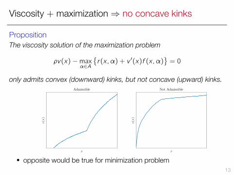
Viscosity + maximization⇒ no concave kinks

PropositionThe viscosity solution of the maximization problem

ρv(x)−maxα∈A

{r(x, α) + v ′(x)f (x, α)

}= 0

only admits convex (downward) kinks, but not concave (upward) kinks.

x

v(x)

Admissible

x

v(x)

Not Admissible

• opposite would be true for minimization problem13

Why is this useful? Problems with non-covexities• Consider growth model

ρv(k) = maxcu(c) + v ′(k)(F (k)− δk − c).

• But drop assumption that F is strictly concave. Instead: “butterfly”F (k) = max{FL(k), FH(k)},FL(k) = ALk

α,

FH(k) = AH((k − κ)+)α, κ > 0, AH > AL

k0 1 2 3 4 5 6

f(k)

0

0.1

0.2

0.3

0.4

0.5

0.6

0.7

0.8

0.9

Figure: Convex-Concave Production

14

Why is this useful? Problems with non-covexities

• Suppose restrict attention to solutions v with at most one kink• there is solution we found in Lecture 3 with convex kink

k

1 2 3 4 5

s(k)

-0.1

-0.08

-0.06

-0.04

-0.02

0

0.02

0.04

0.06

0.08

0.1

(a) Saving Policy Functionk

1 2 3 4 5

v(k)

-90

-80

-70

-60

-50

-40

-30

(b) Value Function

• but there is another solution with a concave kink!

• Proposition above rules out second solution15

Proof that no concave kinks• Step 1: maximization problem⇒ convex Hamiltonian• Step 2: convex Hamiltonian⇒ no concave kinks• Proof of Step 1: Hamiltonian is

H(x, p) := maxα∈A{r(x, α) + pf (x, α)}

• first- and second-order conditions:rα + pfα = 0 (FOC)

rαα + pfαα ≤ 0 (SOC)• From (FOC)

αp = −fα

(rαα + pfαα)

• Differentiating Hamiltonian, we have Hp(x, p) = f (x, α(x, p)) and

Hpp = fααp = −(fα)

2

(rαα + pfαα)> 0

16

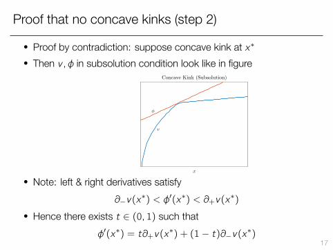
Proof that no concave kinks (step 2)

• Proof by contradiction: suppose concave kink at x∗

• Then v , ϕ in subsolution condition look like in figure

x

v

φ

Concave Kink (Subsolution)

• Note: left & right derivatives satisfy∂−v(x

∗) < ϕ′(x∗) < ∂+v(x∗)

• Hence there exists t ∈ (0, 1) such thatϕ′(x∗) = t∂+v(x

∗) + (1− t)∂−v(x∗)17

Proof that no concave kinks (step 2)

• Because H is convex, for t defined on previous slide

H(x∗, ϕ′(x∗)) < tH(x∗, ∂+v′(x∗)) + (1− t)H(x∗, ∂−v ′(x∗)) (∗)

• By continuity of v

ρv(x∗) = H(x∗, ∂+v(x∗)),

ρv(x∗) = H(x∗, ∂−v(x∗))

• Therefore (∗) implies

H(x∗, ϕ′(x∗)) < ρv(x∗)

• But this contradicts the subsolution condition

ρv(x∗) ≤ H(x∗, ϕ′(x∗)). □

18

Something to Keep in Mind

• Viscosity solution can handle problems where v has kinks...

• ... but not discontinuities

• Theory can be extended in special cases, but no general theory ofdiscontinuous viscosity solutions

• In economics, kinks seem more common than discontinuities

• Good reference on HJB equations with discontinuities: Barles andChasseigne (2015) “(Almost) Everything You Always Wanted toKnow About Deterministic Control Problems in Stratified Domains”http://arxiv.org/abs/1412.7556

19

Viscosity Solutions with StateConstraints

20

Constrained Viscosity Soln: Boundary Inequalities

• How handle “state constraints”?• borrowing constraints• computations with bounded domain

• Example: growth model with state constraint

v (k0) = max{c(t)}t≥0

∫ ∞0

e−ρtu(c(t))dt s.t.

k (t) = F (k(t))− δk(t)− c(t)k(t) ≥ kmin all t ≥ 0

• purely pedagogical: constraint will never bind if kmin < st.st.• HJB equation

ρv(k) = maxc

{u(c) + v ′(k)(F (k)− δk − c)

}(HJB)

• Key question: how impose k ≥ kmin?21

Example: Growth Model with Constraint

• Result: if v is (left-)differentiable at kmin, it needs to satisfy

v ′(kmin) ≥ u′(F (kmin)− δkmin) (BI)

• Intuition:• v ′(kmin) is such that if k(t) = kmin then k(t) ≥ 0• if v is differentiable, the FOC still holds at the constraint

u′(c(kmin)) = v′(kmin) (FOC)

• for constraint not to be violated, need

F (kmin)− δkmin − c(kmin) ≥ 0 (∗)

• (FOC) and (∗)⇒ (BI).

• Next: state constraints in generic optimal control problem22

Generic Control Problem with State Constraint

• Consider variant of generic maximization problem

v(x) = max{α(t)}t≥0

∫ ∞0

e−ρtr(x(t), α(t))dt s.t.

x(t) = f (x(t), α(t)), x(0) = x

x(t) ≥ xmin all t ≥ 0

• HJB equation

ρv(x) = maxα∈A

{r(x, α) + v ′(x)f (x, α)

}(HJB)

• Question: how impose x ≥ xmin? Two cases:

1. v is (left-)differentiable at xmin: boundary inequality2. v not differentiable at xmin: “constrained viscosity solution”

23

State constraints if v is differentiable

• Use Hamiltonian formulation

ρv(x) = H(x, v ′(x)) (HJB)H(x, p) := max

α∈A{r(x, α) + pf (x, α)} (H)

• From envelope condition

Hp(x, v′(x)) = f (x, α∗(x)) = optimal drift at x

• If v ′ and Hp exist, (HJB) for generic control problem satisfies

Hp(xmin, v′(xmin)) ≥ 0 (BI)

• see Soner (1986, p.553) and Fleming and Soner (2006, p.108)• write state constraint as f (x, α∗(x)) · ν(x) ≤ 0 for x at

boundary where ν(x) = “outward normal vector” at boundary• show this implies Hp(x,∇v(x)) · ν(x) ≥ 0

24

If v not differentiable: constrained viscosity solution• Setting Hp(xmin, v ′(xmin)) ≥ 0 obviously requires v to be

(left-)differentiable⇒ what if not differentiable at xmin?

• Definition: a constrained viscosity solution of (HJB) is a continuousfunction v such that

1. v is a viscosity solution (i.e. both sub- and supersolution) forall x > xmin

2. v is a subsolution at x = xmin: if ϕ is any smooth function andif v − ϕ has a local maximum at point xmin, then

ρv(xmin) ≤ maxα∈A

{r(xmin, α) + ϕ

′(xmin)f (xmin, α)}

(∗)

• (∗) functions as boundary condition, or rather “boundary inequality”

• Note: minimization⇒ opposite, i.e. supersolution at boundary• for minimization: Fleming and Soner (2006), Section II.12• for maximization: e.g. Definition 3.1 in Zariphopoulou (1994)

25

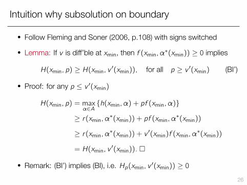
Intuition why subsolution on boundary

• Follow Fleming and Soner (2006, p.108) with signs switched

• Lemma: If v is diff’ble at xmin, then f (xmin, α∗(xmin)) ≥ 0 implies

H(xmin, p) ≥ H(xmin, v ′(xmin)), for all p ≥ v ′(xmin) (BI’)

• Proof: for any p ≤ v ′(xmin)

H(xmin, p) = maxα∈A{h(xmin, α) + pf (xmin, α)}

≥ r(xmin, α∗(xmin)) + pf (xmin, α∗(xmin))

≥ r(xmin, α∗(xmin)) + v ′(xmin)f (xmin, α∗(xmin))

= H(xmin, v′(xmin)). □

• Remark: (BI’) implies (BI), i.e. Hp(xmin, v ′(xmin)) ≥ 026

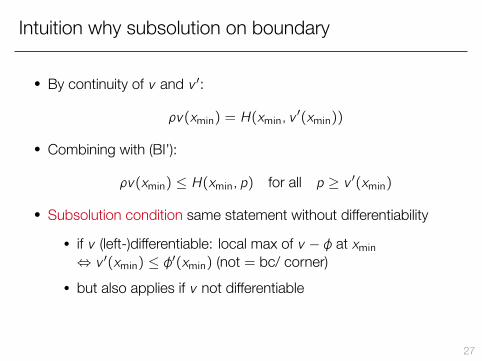
Intuition why subsolution on boundary

• By continuity of v and v ′:

ρv(xmin) = H(xmin, v′(xmin))

• Combining with (BI’):

ρv(xmin) ≤ H(xmin, p) for all p ≥ v ′(xmin)

• Subsolution condition same statement without differentiability

• if v (left-)differentiable: local max of v − ϕ at xmin⇔ v ′(xmin) ≤ ϕ′(xmin) (not = bc/ corner)

• but also applies if v not differentiable

27

Example: Growth Model with Bounded Domain

• Consider again HJB equation for growth model

ρv(k) = maxc

{u(c) + v ′(k)(F (k)− δk − c)

}• For numerical solution, want to impose

kmin ≤ k(t) ≤ kmax all t

• How can we ensure this?

• Answer: impose two boundary inequalities

v ′(kmin)≥u′(F (kmin)− δkmin)

v ′(kmax)≤u′(F (kmax)− δkmax)

28

Uniqueness of Viscosity Solution

29

Uniqueness of Viscosity Solution

• Theorem: Under some conditions, HJB equation has uniqueviscosity solution

• due to Crandall and Lions (1983), “Viscosity Solutions ofHamilton-Jacobi Equations”

• My intuition for uniqueness theorem with state constraints in onedimension

• ODE has unique solution given one boundary condition• two boundary inequalities = one boundary condition ...• ... sufficient to pin down unique solution

• but much more powerful: generalizes to N dimensions, kinks etc

30

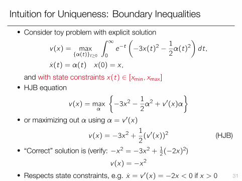
Intuition for Uniqueness: Boundary Inequalities• Consider toy problem with explicit solution

v(x) = max{α(t)}t≥0

∫ ∞0

e−t(−3x(t)2 −

1

2α(t)2

)dt,

x(t) = α(t) x(0) = x,

and with state constraints x(t) ∈ [xmin, xmax]• HJB equation

v(x) = maxα

{−3x2 −

1

2α2 + v ′(x)α

}• or maximizing out α using α = v ′(x)

v(x) = −3x2 +1

2(v ′(x))2 (HJB)

• “Correct” solution is (verify: −x2 = −3x2 + 12(−2x)2)v(x) = −x2

• Respects state constraints, e.g. x = v ′(x) = −2x < 0 if x > 0 31

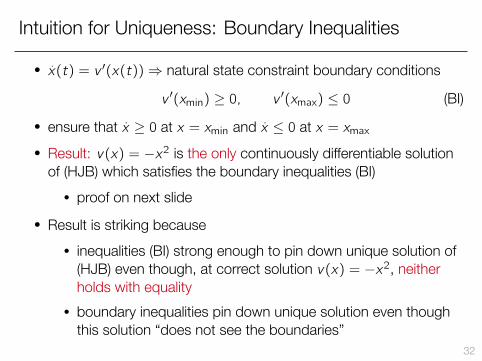
Intuition for Uniqueness: Boundary Inequalities

• x(t) = v ′(x(t))⇒ natural state constraint boundary conditions

v ′(xmin) ≥ 0, v ′(xmax) ≤ 0 (BI)

• ensure that x ≥ 0 at x = xmin and x ≤ 0 at x = xmax• Result: v(x) = −x2 is the only continuously differentiable solution

of (HJB) which satisfies the boundary inequalities (BI)• proof on next slide

• Result is striking because• inequalities (BI) strong enough to pin down unique solution of

(HJB) even though, at correct solution v(x) = −x2, neitherholds with equality

• boundary inequalities pin down unique solution even thoughthis solution “does not see the boundaries”

32

Proof of Result• Let v be smooth solution of (HJB). Let v(0) = c . Rule out c = 0• Easy to rule out c < 0: (HJB) at x = 0 is c = 1

2(v′(0))2 ⇒ no

solution for v ′(0) when c < 0• Next consider c > 0. Inverting (HJB) for v ′ yields two branches

Branch 1: v ′(x) = +√6x2 + 2v(x)

Branch 2: v ′(x) = −√6x2 + 2v(x)

• Importantly, continuous v ′ ⇒ v satisfies either branch 1 or branch2 for all x ∈ (xmin, xmax), i.e. cannot switch branches

• in particular c > 0⇒ switching branches not allowed at x = 0• Suppose v satisfies branch 1 for all x . Then

• v ′(0) =√2c > 0 and v(x) > c for x > 0 near x = 0

• Similarly v(x) > c, v ′(x) > 0 all x > 0⇒ violate v ′(xmax) ≤ 0• Suppose v satisfies branch 2 for all x . Then v ′(0) = −

√2c < 0 ...

• ... v(x) > c, v ′(x) < 0 all x < 0⇒ violate v ′(xmin) ≥ 0 □ 33

Remark: strengthening the result

• Have restricted attention to solutions such that v ′ is continuous

• In fact, result can be strengthened further to say

• Result 2: v(x) = −x2 is the only solution of (HJB) without concavekinks (“viscosity solution”) which satisfies boundary inequalities (BI)

34

Uniqueness Theorem: Logic

• Here outline case with state constraints: x ∈ [xmin, xmax]• due to Soner (1986), Capuzzo-Dolcetta & Lions (1990)• use notation X := (xmin, xmax) and X := [xmin, xmax]• can extend to unbounded domain x ∈ R (references later)

• Key step in uniqueness proof: “comparison theorem”• Consider HJB equation

ρv(x) = maxα∈A

{r(x, α) + v ′(x)f (x, α)

}(HJB)

with state constraints x ∈ X• Comparisontheorem: (Under certain assumptions...) if v1 is

subsolution of (HJB) on X & v2 is supersolution of (HJB) on X, then

v1(x) ≤ v2(x) for all x ∈ X.35

Remark: another comparison theorem you may know

• Here’s another comparison theorem you may know that has samestructure: Grönwall’s inequality

• If v ′1(t) ≤ β(t)v1(t) then v1(t) ≤ v1(0) exp(∫ t0 β(s)ds

)• This is really: If v ′1(t)≤β(t)v1(t) and v ′2(t)=β(t)v2(t), then

v1(t) ≤ v2(t) for all t

36

Comparison Theorem immediately⇒ Uniqueness

• Corollary (uniqueness): there exists a unique constrained viscositysolution of (HJB) on X, i.e. if v1 and v2 are both constrainedviscosity solutions of (HJB) on X, then v1(x) = v2(x) for all x ∈ X

• Proof: let v1, v2 be constrained viscosity solutions of (HJB) on X

1. Since v1 and v2 are constrained viscosity solutions, v1 is also asubsolution on X and v2 is a supersolution on X. By thecomparison theorem, therefore v1(x) ≤ v2(x) for all x ∈ X

2. Reversing roles of v1, v2 in (1)⇒ v2(x) ≤ v1(x) for all x ∈ X

3. (1) and (2) imply v1(x) = v2(x) for all x ∈ X, i.e. uniqueness.□

37

Proof Sketch of Comparison Thm with smooth v1, v2

• Thm: v1 = subsolution, v2 = supersolution⇒ v1(x) ≤ v2(x) all x

• Proof by contradiction: suppose instead v1(x) > v2(x) for some x

• ... equivalently, v1 − v2 attains local maximum at some pointx∗ ∈ X with v1(x∗) > v2(x∗)

• Two cases:1. x∗ in interior: x∗ ∈ X2. x∗ on boundary: x∗ = xmin or x∗ = xmax

• Here: ignore case 2, i.e. possibility of x∗ on boundary

• requires more work, just like non-smooth v1, v2• for complete proof, see references

38

Proof Sketch of Comparison Thm with smooth v1, v2

• If v1 − v2 attains local maximum at interior x∗, then since v1, v2 aresmooth also v ′1(x∗) = v ′2(x∗)

• v1 is subsolution means: for any smooth ϕ and x∗ such that v1 − ϕattains local max: ρv1(x∗) ≤ maxα∈A {r(x∗, α) + ϕ′(x∗)f (x∗, α)}

• In particular, use ϕ = v2:ρv1(x

∗) ≤ maxα∈A

{r(x∗, α) + v ′2(x

∗)f (x∗, α)}

(1)

• Repeat symmetric steps with supersolution condition for v2, settingϕ = v1 and noting that v2 − v1 attains local min at x∗

ρv2(x∗) ≥ max

α∈A

{r(x∗, α) + v ′1(x

∗)f (x∗, α)}

(2)

• Subtracting (2) from (1) and recalling v ′1(x∗) = v ′2(x∗) we havev1(x

∗) ≤ v2(x∗). Contradiction.□39

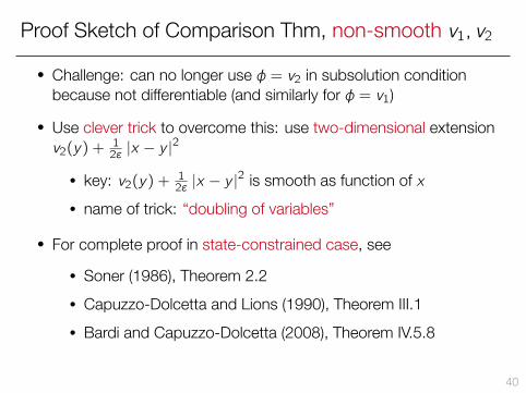
Proof Sketch of Comparison Thm, non-smooth v1, v2

• Challenge: can no longer use ϕ = v2 in subsolution conditionbecause not differentiable (and similarly for ϕ = v1)

• Use clever trick to overcome this: use two-dimensional extensionv2(y) +

12ε |x − y |

2

• key: v2(y) + 12ε |x − y |

2 is smooth as function of x• name of trick: “doubling of variables”

• For complete proof in state-constrained case, see

• Soner (1986), Theorem 2.2• Capuzzo-Dolcetta and Lions (1990), Theorem III.1• Bardi and Capuzzo-Dolcetta (2008), Theorem IV.5.8

40

Variants on Comparison Theorem (still⇒ Uniqueness)

1. Known values of v at xmin, xmax (“Dirichlet boundary conditions”)• simplest case and the one covered in most textbooks, notes• kind of uninteresting, mostly useful for understanding proof

strategy• Yu (2011), Section 3• Bressan (2011), Theorem 5.1

2. Unbounded domain x ∈ R• just like in discrete time, need certain boundedness

assumptions on v1, v2 (e.g. at most linear growth)• Sections 5 and 6 of Crandall (1995)• Theorem III.2.12 in Bardi & Capuzzo-Dolcetta (2008)

41

Additional Results on HJB Equation in Economics

• Strulovici and Szydlowski (2015) “On the smoothness of valuefunctions and the existence of optimal strategies in diffusionmodels”

• very nice analysis of one-dimensional case (note: does notapply to N > 1)

• provide conditions under which v is twice differentiable...

• ... in which case whole viscosity apparatus not needed

• no uniqueness result...• ... but they note that uniqueness implied because v=solution

to “sequence problem” which has unique solution

42