virtual water imports: using agricultural trade to cope ... · virtual water imports: using...
TRANSCRIPT
Virtual Water Imports: Using Agricultural Trade to Copewith Water Scarcity
Miguel Cardenas Rodriguez1 and Alban Thomas2
1OECD, Paris2Toulouse School of Economics (LERNA, INRA)
Conference Noviwam, January 21, 2013
Miguel Cardenas Rodriguez and Alban Thomas ( OECD, Paris Toulouse School of Economics (LERNA, INRA))NoviWam, January 21 2013, Sevilla 21/01/2013 1 / 36
1 Introduction
2 Virtual Water: Definition and Concepts
3 Literature
4 Empirical Application
5 Conclusion
Miguel Cardenas Rodriguez and Alban Thomas ( OECD, Paris Toulouse School of Economics (LERNA, INRA))NoviWam, January 21 2013, Sevilla 21/01/2013 2 / 36
Introduction
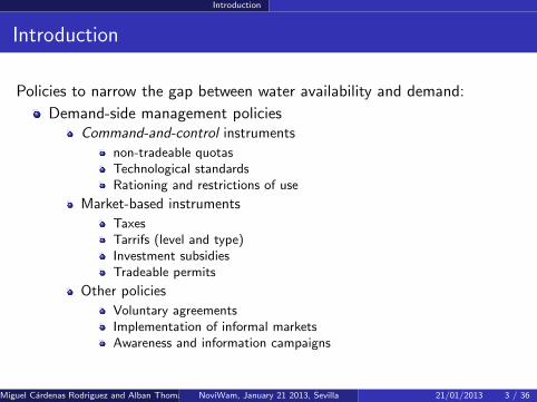
Introduction
Policies to narrow the gap between water availability and demand:
Demand-side management policiesCommand-and-control instruments
non-tradeable quotasTechnological standardsRationing and restrictions of use
Market-based instruments
TaxesTarrifs (level and type)Investment subsidiesTradeable permits
Other policies
Voluntary agreementsImplementation of informal marketsAwareness and information campaigns
Miguel Cardenas Rodriguez and Alban Thomas ( OECD, Paris Toulouse School of Economics (LERNA, INRA))NoviWam, January 21 2013, Sevilla 21/01/2013 3 / 36
Introduction
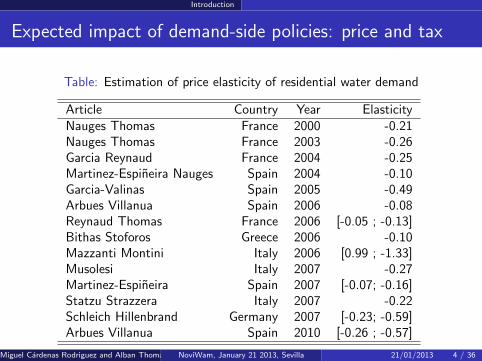
Expected impact of demand-side policies: price and tax
Table: Estimation of price elasticity of residential water demand
Article Country Year ElasticityNauges Thomas France 2000 -0.21Nauges Thomas France 2003 -0.26Garcia Reynaud France 2004 -0.25Martinez-Espineira Nauges Spain 2004 -0.10Garcia-Valinas Spain 2005 -0.49Arbues Villanua Spain 2006 -0.08Reynaud Thomas France 2006 [-0.05 ; -0.13]Bithas Stoforos Greece 2006 -0.10Mazzanti Montini Italy 2006 [0.99 ; -1.33]Musolesi Italy 2007 -0.27Martinez-Espineira Spain 2007 [-0.07; -0.16]Statzu Strazzera Italy 2007 -0.22Schleich Hillenbrand Germany 2007 [-0.23; -0.59]Arbues Villanua Spain 2010 [-0.26 ; -0.57]
Miguel Cardenas Rodriguez and Alban Thomas ( OECD, Paris Toulouse School of Economics (LERNA, INRA))NoviWam, January 21 2013, Sevilla 21/01/2013 4 / 36
Introduction
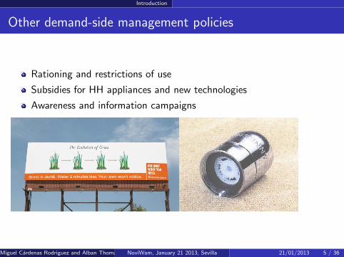
Other demand-side management policies
Rationing and restrictions of use
Subsidies for HH appliances and new technologies
Awareness and information campaigns
Miguel Cardenas Rodriguez and Alban Thomas ( OECD, Paris Toulouse School of Economics (LERNA, INRA))NoviWam, January 21 2013, Sevilla 21/01/2013 5 / 36
Introduction
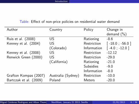
Table: Effect of non-price policies on residential water demand
Author Country Policy Change indemand (%)
Ruis et al. (2008) US Rationing -8.6Kenney et al. (2004) US Restriction [ -18.0 ; -56.0 ]
(Colorado) Information [ -4.0 ; -12.0 ]Kenney et al. (2008) US Restriction -12.12Renwick Green (2000) US Restriction -29.0
(California) Rationing -21.0Subsidies -9.0Information -8.0
Grafton Kompas (2007) Australia (Sydney) Restriction -10.0Bartczak et al. (2009) Poland Meters -20.0
Miguel Cardenas Rodriguez and Alban Thomas ( OECD, Paris Toulouse School of Economics (LERNA, INRA))NoviWam, January 21 2013, Sevilla 21/01/2013 6 / 36
Introduction
or
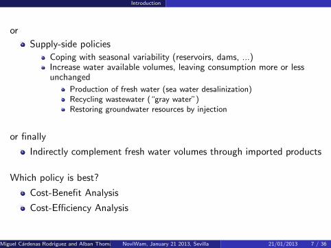
Supply-side policies
Coping with seasonal variability (reservoirs, dams, ...)Increase water available volumes, leaving consumption more or lessunchanged
Production of fresh water (sea water desalinization)Recycling wastewater (“gray water”)Restoring groundwater resources by injection
or finally
Indirectly complement fresh water volumes through imported products
Which policy is best?
Cost-Benefit Analysis
Cost-Efficiency Analysis
Miguel Cardenas Rodriguez and Alban Thomas ( OECD, Paris Toulouse School of Economics (LERNA, INRA))NoviWam, January 21 2013, Sevilla 21/01/2013 7 / 36
Introduction
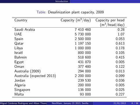
Table: Desalinization plant capacity, 2009
Country Capacity (m3/day) Capacity per head(m3/head/day)
Saudi Arabia 7 410 460 0.28UAE 5 730 000 1.07Spain 2 500 000 0.053Qatar 1 197 150 0.613Libya 1 000 000 0.178Israel 800 000 0.105Bahrein 518 600 0.415Egypt 431 870 0.005Oman 377 480 0.122Australia (2009) 294 000 0.013Australia (expected 2013) 2 200 000 0.099Jordan 239 530 0.036Algeria 200 000 0.005Singapore 136 000 0.025Malta 93 000 0.227
Miguel Cardenas Rodriguez and Alban Thomas ( OECD, Paris Toulouse School of Economics (LERNA, INRA))NoviWam, January 21 2013, Sevilla 21/01/2013 8 / 36

Introduction
Cost-efficiency analysis: example of Algeria
Emergency programme of seawater desalinization adopted in 2002
Objectif towards 2030: 2.2 million m3/day
Cost-efficiency analysis: comparison of two strategies
supply-side management: seawater desalinization (the current plan)demand-side management: promote a more efficient irrigationDuration: 20 years (discount rate 8 %)
Akli, S. and S. Bedrani, Cahiers du CREAD, 96, 2011.
Desalinization Irrigation
• Eight single-block stations • Irrigation (fruit trees), West MitidjaInverse osmosis • Yield drip irrigation: 35 %• Production 4.58 Mm3/year • Same reduction objective• Return 60 % Area considered 1852 ha• Cost: 68.34 DA/m3 • Saving: 8.59 DA/m3
(0.66 euro/m3) (0.08 euro/m3)
Miguel Cardenas Rodriguez and Alban Thomas ( OECD, Paris Toulouse School of Economics (LERNA, INRA))NoviWam, January 21 2013, Sevilla 21/01/2013 9 / 36

Virtual Water: Definition and Concepts
Virtual Water: Definition and Concepts
Variable DefinitionVirtual water Water used for the production of a good or
service, not visible in the final productVirtual water content Volume of fresh water consumed or pollutedof a product for producing a productWater Footprint Multi dimensional indicator of freshwater use
(both direct and indirect) by a consumer or producerBlue water Fresh surface or groundwaterGreen water Precipitation on land that does not run off or recharge
the groundwater but is stored in the soilor temporarily stays on top of the soil or vegetation
Grey water Volume of polluted water flow, aquifers and rivers
Miguel Cardenas Rodriguez and Alban Thomas ( OECD, Paris Toulouse School of Economics (LERNA, INRA))NoviWam, January 21 2013, Sevilla 21/01/2013 10 / 36
Virtual Water: Definition and Concepts
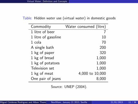
Table: Hidden water use (virtual water) in domestic goods
Commodity Water consumed (litre)
1 litre of beer 71 litre of gasoline 101 cola 70A single bath 2001 kg of paper 3201 kg of bread 1,0001 kg of potatoes 1,000Television set 1,0001 kg of meat 4,000 to 10,000One pair of jeans 8,000
Source: UNEP (2004).
Miguel Cardenas Rodriguez and Alban Thomas ( OECD, Paris Toulouse School of Economics (LERNA, INRA))NoviWam, January 21 2013, Sevilla 21/01/2013 11 / 36
Virtual Water: Definition and Concepts
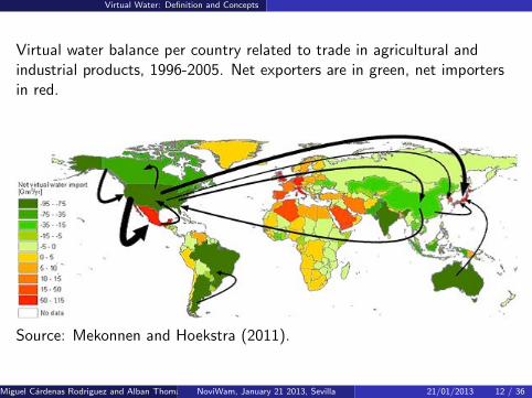
Virtual water balance per country related to trade in agricultural andindustrial products, 1996-2005. Net exporters are in green, net importersin red.
Source: Mekonnen and Hoekstra (2011).
Miguel Cardenas Rodriguez and Alban Thomas ( OECD, Paris Toulouse School of Economics (LERNA, INRA))NoviWam, January 21 2013, Sevilla 21/01/2013 12 / 36

Virtual Water: Definition and Concepts
The case of crops
Focus on crops because of agriculture a major water user
Crop Virtual Water content (m3/t) =Crop Water Requirement(m3/ha)
Crop Yield(t/ha)
Table: Examples of Water Footprint in m3/ton
Country Wheat Maize
Green Blue Grey Green Blue Grey
France 581.24 1.33 5.50 425.92 92.21 156.44Mexico 332.81 558.29 184.71 1851.85 61.76 356.95Global average 1277.21 342.46 207.42 947.20 81.23 193.93
Miguel Cardenas Rodriguez and Alban Thomas ( OECD, Paris Toulouse School of Economics (LERNA, INRA))NoviWam, January 21 2013, Sevilla 21/01/2013 13 / 36
Virtual Water: Definition and Concepts
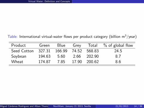
Table: International virtual-water flows per product category (billion m3/year)
Product Green Blue Grey Total % of global flow
Seed Cotton 327.31 166.99 74.52 568.83 24.5Soybean 194.63 5.60 2.66 202.90 8.7Wheat 174.87 7.85 17.90 200.62 8.6
Miguel Cardenas Rodriguez and Alban Thomas ( OECD, Paris Toulouse School of Economics (LERNA, INRA))NoviWam, January 21 2013, Sevilla 21/01/2013 14 / 36
Virtual Water: Definition and Concepts
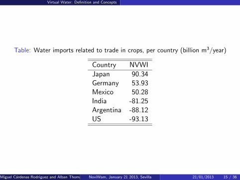
Table: Water imports related to trade in crops, per country (billion m3/year)
Country NVWI
Japan 90.34Germany 53.93Mexico 50.28India -81.25Argentina -88.12US -93.13
Miguel Cardenas Rodriguez and Alban Thomas ( OECD, Paris Toulouse School of Economics (LERNA, INRA))NoviWam, January 21 2013, Sevilla 21/01/2013 15 / 36
Virtual Water: Definition and Concepts
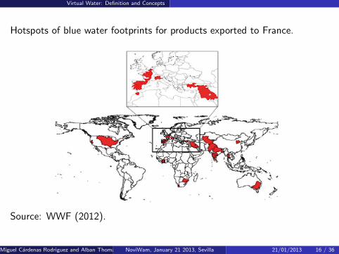
Hotspots of blue water footprints for products exported to France.
Source: WWF (2012).
Miguel Cardenas Rodriguez and Alban Thomas ( OECD, Paris Toulouse School of Economics (LERNA, INRA))NoviWam, January 21 2013, Sevilla 21/01/2013 16 / 36
Virtual Water: Definition and Concepts
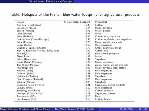
Table: Hotspots of the French blue water footprint for agricultural products
Region % Blue Water Footprint Product(s)Aral Sea (Uzbekistan) 6.38 CottonGaronne (France) 5.44 Maize, soybeanEscaut (France) 4.46 Maize, potatoLoire (France) 4.43 MaizeIndus (Pakistan) 3.85 Cotton, rice, sugarcaneGuadalquivir (Spain-Portugal) 2.98 Cotton, sunflower, rice, sugarbeetSeine (France) 2.23 Maize, potato, sugarbeetGange (India) 2.19 Rice, sugarcaneGuadiana (Spain-Portugal) 1.79 Grape, sunflower, citrusTiger & Euphrate (Turkey, Syria, Iraq) 1.62 Cotton, ricePo (Italy) 1.59 Rice, animal productsEbro (Spain) 1.39 MaizeSebou (Morocco) 1.39 SugarbeetDouro (Spain-Portugal) 1.29 Maize, sugarbeetTejo (Spain-Portugal) 1.02 grape, maize, animal productsMississippi (US) 0.60 Maize, soybean, rice, cottonKrishna (India) 0.45 Rice, sugarcaneGodavari (India) 0.31 Rice, sugarcaneKizilirmak (Turkey) 0.27 SugarbeetChao Phraya (Thailand) 0.26 Rice, sugarcaneSakarya (Turkey) 0.25 SugarbeetBandama (Cote d’Ivoire) 0.21 Sugarcane, animal productsCauvery (India) 0.19 Rice, sugarcaneYongding He (China) 0.12 Cotton, soybeanLimpopo (SOuth Africa) 0.11 Sugarcane, cottonSacramento (US) 0.10 RiceSan Joaquin (US) 0.10 Cotton, Maize
Miguel Cardenas Rodriguez and Alban Thomas ( OECD, Paris Toulouse School of Economics (LERNA, INRA))NoviWam, January 21 2013, Sevilla 21/01/2013 17 / 36
Literature
Literature
Almost no theoretical analysis
focus on computing virtual water coefficients and its relevance ininternational water policy making
Use of international trade theories (Ricardian Model of comparativeadvantages, Hecksher-Ohlin): Tomini (2009), Zimmer and Renault(2003)
Hoekstra and Hung (2002), Mekonnen and Hoekstra (2010),Chapagain and Hoekstra (2006), Ocki and Kanae (2003), Wichelns(2006): study on virtual water content for major crops, livestock andindustrial products.
Since 2008, Water Footprint Network website: update databases
International water policy: Warner (2002) and Allan (2003) on waterwars and stronger interdependency to eliminate conflicts
Miguel Cardenas Rodriguez and Alban Thomas ( OECD, Paris Toulouse School of Economics (LERNA, INRA))NoviWam, January 21 2013, Sevilla 21/01/2013 18 / 36
Literature
The literature on virtual water points out to globalization of waterresources and advocates for trade liberalization in order to managewater resources globally and enhance food security
Yang et al (2003): below threshold of 1500 m3/head/year, thedemand for cereal import from Asia and Afria increases exponentially
Hoekstra and Hung (2002): no apparent relationship between waterresources and net imports of virtual water
But this study fails to acknowledge the importance of determinants ofdemand for agricultural virtual water: agricultural land, irrigationsystems, income, diet habits and availability of various types of water.
Miguel Cardenas Rodriguez and Alban Thomas ( OECD, Paris Toulouse School of Economics (LERNA, INRA))NoviWam, January 21 2013, Sevilla 21/01/2013 19 / 36
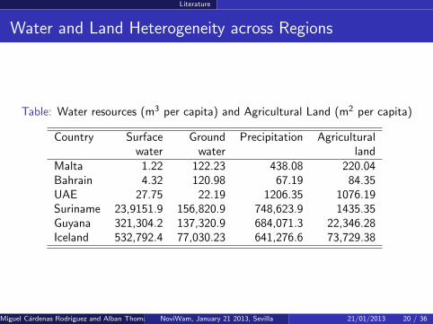
Literature
Water and Land Heterogeneity across Regions
Table: Water resources (m3 per capita) and Agricultural Land (m2 per capita)
Country Surface Ground Precipitation Agriculturalwater water land
Malta 1.22 122.23 438.08 220.04Bahrain 4.32 120.98 67.19 84.35UAE 27.75 22.19 1206.35 1076.19Suriname 23,9151.9 156,820.9 748,623.9 1435.35Guyana 321,304.2 137,320.9 684,071.3 22,346.28Iceland 532,792.4 77,030.23 641,276.6 73,729.38
Miguel Cardenas Rodriguez and Alban Thomas ( OECD, Paris Toulouse School of Economics (LERNA, INRA))NoviWam, January 21 2013, Sevilla 21/01/2013 20 / 36
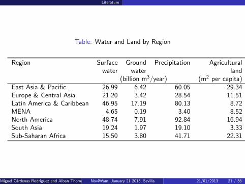
Literature
Table: Water and Land by Region
Region Surface Ground Precipitation Agriculturalwater water land
(billion m3/year) (m2 per capita)East Asia & Pacific 26.99 6.42 60.05 29.34Europe & Central Asia 21.20 3.42 28.54 11.51Latin America & Caribbean 46.95 17.19 80.13 8.72MENA 4.65 0.19 3.40 8.52North America 48.74 7.91 92.84 16.94South Asia 19.24 1.97 19.10 3.33Sub-Saharan Africa 15.50 3.80 41.71 22.31
Miguel Cardenas Rodriguez and Alban Thomas ( OECD, Paris Toulouse School of Economics (LERNA, INRA))NoviWam, January 21 2013, Sevilla 21/01/2013 21 / 36
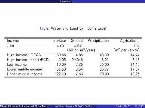
Literature
Table: Water and Land by Income Level
Income Surface Ground Precipitation Agriculturalclass water water land
(billion m3/year) (m2 per capita)High income: OECD 30.66 4.86 48.39 14.24High income: non-OECD 2.05 0.4046 8.21 5.45Low income 10.09 2.36 26.00 14.45Lower middle income 31.53 8.54 56.77 17.87Upper middle income 22.70 7.68 50.90 18.96
Miguel Cardenas Rodriguez and Alban Thomas ( OECD, Paris Toulouse School of Economics (LERNA, INRA))NoviWam, January 21 2013, Sevilla 21/01/2013 22 / 36
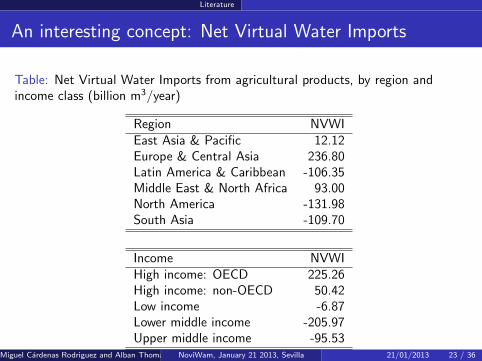
Literature
An interesting concept: Net Virtual Water Imports
Table: Net Virtual Water Imports from agricultural products, by region andincome class (billion m3/year)
Region NVWIEast Asia & Pacific 12.12Europe & Central Asia 236.80Latin America & Caribbean -106.35Middle East & North Africa 93.00North America -131.98South Asia -109.70
Income NVWIHigh income: OECD 225.26High income: non-OECD 50.42Low income -6.87Lower middle income -205.97Upper middle income -95.53
Miguel Cardenas Rodriguez and Alban Thomas ( OECD, Paris Toulouse School of Economics (LERNA, INRA))NoviWam, January 21 2013, Sevilla 21/01/2013 23 / 36
Empirical Application
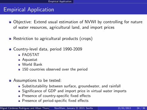
Empirical Application
Objective: Extend usual estimation of NVWI by controlling for natureof water resources, agricultural land, and import prices
Restriction to agricultural products (crops)
Country-level data, period 1990-2009FAOSTATAquastatWorld Bank150 countries observed over the period
Assumptions to be tested:Substitutability between surface, groundwater, and rainfallSignificance of GDP and import price in virtual water importsPresence of country-specific fixed effectsPresence of period-specific fixed effects
Miguel Cardenas Rodriguez and Alban Thomas ( OECD, Paris Toulouse School of Economics (LERNA, INRA))NoviWam, January 21 2013, Sevilla 21/01/2013 24 / 36
Empirical Application
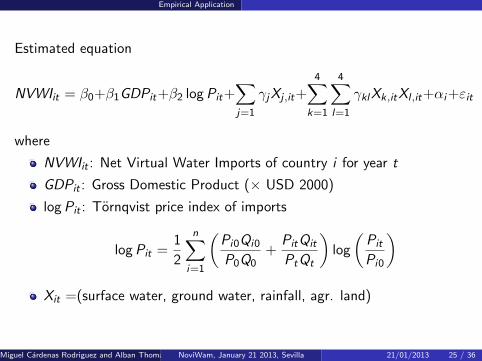
Estimated equation
NVWIit = β0+β1GDPit+β2 logPit+∑j=1
γjXj ,it+4∑
k=1
4∑l=1
γklXk,itXl ,it+αi+εit
where
NVWIit : Net Virtual Water Imports of country i for year t
GDPit : Gross Domestic Product (× USD 2000)
logPit : Tornqvist price index of imports
logPit =1
2
n∑i=1
(Pi0Qi0
P0Q0+
PitQit
PtQt
)log
(Pit
Pi0
)Xit =(surface water, ground water, rainfall, agr. land)
Miguel Cardenas Rodriguez and Alban Thomas ( OECD, Paris Toulouse School of Economics (LERNA, INRA))NoviWam, January 21 2013, Sevilla 21/01/2013 25 / 36
Empirical Application
Surface Water: the sum of internal renewable water resources andexternal actual renewable water resources. It corresponds to themaximum theoretical yearly amount of water actually available for acountry at a given moment. Measured in cubic meters per capita perperiod. Defined by the AQUASTAT database from FAO
Groundwater: the sum of the internal renewable groundwaterresources and the total external actual renewable groundwaterresources. Measured in cubic meters per capita per period
Precipitation: the long-term average, over space and time, of annualendogenous precipitation in volume produced in the country.Measured in cubic meters per capita per period
Agricultural Land: the sum of areas under arable land, permanentcrops and permanent meadows and pastures. Measured in squaredmeters per capita per period
Miguel Cardenas Rodriguez and Alban Thomas ( OECD, Paris Toulouse School of Economics (LERNA, INRA))NoviWam, January 21 2013, Sevilla 21/01/2013 26 / 36
Empirical Application
Countries classified in 7 geographical regions according to the World Bank:
North America
Latin America & Caribbean
Europe & Central Asia
Middle East & North Africa
Sub-Saharan Africa
East Asia & Pacific
South Asia
Divided in 5 income levels according to the World Bank classification
High income: OECD
High income: non OECD
Upper middle income
Lower middle income
Low income
Miguel Cardenas Rodriguez and Alban Thomas ( OECD, Paris Toulouse School of Economics (LERNA, INRA))NoviWam, January 21 2013, Sevilla 21/01/2013 27 / 36
Empirical Application
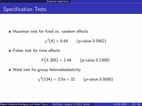
Specification Tests
Hausman test for fixed vs. random effects
χ2(4) = 6.64 (p-value 0.0562)
Fisher test for time effects
F (3, 305) = 1.44 (p-value 0.2309)
Wald test for group heteroskedasticity
χ2(134) = 3.5e + 32 (p-value 0.0000)
Miguel Cardenas Rodriguez and Alban Thomas ( OECD, Paris Toulouse School of Economics (LERNA, INRA))NoviWam, January 21 2013, Sevilla 21/01/2013 28 / 36
Empirical Application
Estimation Results
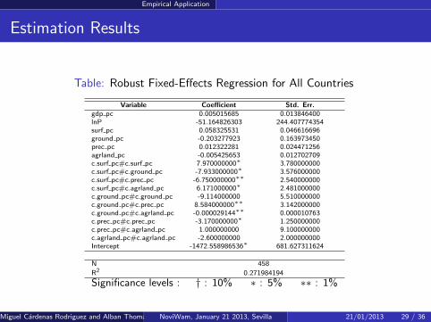
Table: Robust Fixed-Effects Regression for All Countries
Variable Coefficient Std. Err.gdp pc 0.005015685 0.013846400lnP -51.164826303 244.407774354surf pc 0.058325531 0.046616696ground pc -0.203277923 0.163973450prec pc 0.012322281 0.024471256agrland pc -0.005425653 0.012702709c.surf pc#c.surf pc 7.970000000∗ 3.780000000c.surf pc#c.ground pc -7.933000000∗ 3.576000000c.surf pc#c.prec pc -6.750000000∗∗ 2.540000000c.surf pc#c.agrland pc 6.171000000∗ 2.481000000c.ground pc#c.ground pc -9.114000000 5.510000000c.ground pc#c.prec pc 8.584000000∗∗ 3.142000000c.ground pc#c.agrland pc -0.000029144∗∗ 0.000010763c.prec pc#c.prec pc -3.170000000∗ 1.250000000c.prec pc#c.agrland pc 1.000000000 9.100000000c.agrland pc#c.agrland pc -2.600000000 2.000000000Intercept -1472.558986536∗ 681.627311624
N 458
R2 0.271984194
Significance levels : † : 10% ∗ : 5% ∗∗ : 1%
Miguel Cardenas Rodriguez and Alban Thomas ( OECD, Paris Toulouse School of Economics (LERNA, INRA))NoviWam, January 21 2013, Sevilla 21/01/2013 29 / 36
Empirical Application
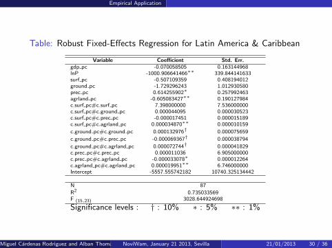
Table: Robust Fixed-Effects Regression for Latin America & Caribbean
Variable Coefficient Std. Err.gdp pc -0.070058505 0.163144968lnP -1000.906641466∗∗ 339.844141633surf pc -0.507109359 0.408194012ground pc -1.729296243 1.012930580prec pc 0.614255902∗ 0.257992463agrland pc -0.605083427∗∗ 0.190127984c.surf pc#c.surf pc 7.398000000 7.536000000c.surf pc#c.ground pc 0.000044095 0.000030523c.surf pc#c.prec pc -0.000017451 0.000015189c.surf pc#c.agrland pc 0.000034870∗∗ 0.000010159
c.ground pc#c.ground pc 0.000132976† 0.000075659
c.ground pc#c.prec pc -0.000069367† 0.000038794
c.ground pc#c.agrland pc 0.000072744† 0.000041829c.prec pc#c.prec pc 0.000011036 6.905000000c.prec pc#c.agrland pc -0.000033078∗ 0.000012264c.agrland pc#c.agrland pc 0.000019951∗∗ 6.746000000Intercept -5557.555742182 10740.325134442
N 87
R2 0.735033569F (15,23) 3028.644924698
Significance levels : † : 10% ∗ : 5% ∗∗ : 1%
Miguel Cardenas Rodriguez and Alban Thomas ( OECD, Paris Toulouse School of Economics (LERNA, INRA))NoviWam, January 21 2013, Sevilla 21/01/2013 30 / 36
Empirical Application
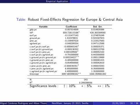
Table: Robust Fixed-Effects Regression for Europe & Central Asia
Variable Coefficient Std. Err.gdp pc -0.007514859 0.014929366
lnP 859.728115186† 426.363309580surf pc -0.131477143 0.274876249ground pc 1.410378831 0.924347923prec pc -0.159497620 0.215527693agrland pc -0.048209354 0.047112588
c.surf pc#c.surf pc -0.000065140† 0.000035371c.surf pc#c.ground pc -0.000136352 0.000122700c.surf pc#c.prec pc 0.000109560∗ 0.000052102c.surf pc#c.agrland pc -9.791000000 8.442000000c.ground pc#c.ground pc 0.000334027∗∗ 0.000119989c.ground pc#c.prec pc -6.485000000 0.000081415c.ground pc#c.agrland pc -9.854000000 0.000042610
c.prec pc#c.prec pc -0.000036351† 0.000019283c.prec pc#c.agrland pc 8.655000000 8.355000000c.agrland pc#c.agrland pc 4.400000000 1.263000000Intercept 3097.865998342∗∗ 1044.359981492
N 143
R2 0.299298936
Significance levels : † : 10% ∗ : 5% ∗∗ : 1%
Miguel Cardenas Rodriguez and Alban Thomas ( OECD, Paris Toulouse School of Economics (LERNA, INRA))NoviWam, January 21 2013, Sevilla 21/01/2013 31 / 36

Empirical Application
Elasticity of Net Virtual Water Imports
Table: Water and Land by Region
Elasticity of NVWI wrt.Region GDP P surface ground rainfall agr. land
water waterAll -0.0085 0.0710 -0.6718 0.6387 0.0123 0.0050Latin America 0.1186 1.3894 -0.0125 0.4779 0.0807 -0.0979Europe & Central Asia 0.0127 -1.1934 -1.4187 -0.0661 6.9633 -0.2758MENA 0.0288 -0.6227 -5.6888 6.3683 -17.1350 9.0868Sub Saharan Africa -0.1348 0.2655 0.0359 -0.0240 0.0769 -0.0005Eastern Asia & Pacific 0.0119 -0.2997 -5.4194 2.8106 0.6096 2.3292
Miguel Cardenas Rodriguez and Alban Thomas ( OECD, Paris Toulouse School of Economics (LERNA, INRA))NoviWam, January 21 2013, Sevilla 21/01/2013 32 / 36
Empirical Application
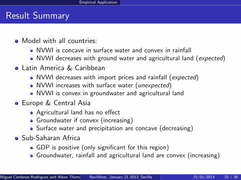
Result Summary
Model with all countries:
NVWI is concave in surface water and convex in rainfallNVWI decreases with ground water and agricultural land (expected)
Latin America & Caribbean
NVWI decreases with import prices and rainfall (expected)NVWI increases with surface water (unexpected)NVWI is convex in groundwater and agricultural land
Europe & Central Asia
Agricultural land has no effectGroundwater if convex (increasing)Surface water and precipitation are concave (decreasing)
Sub-Saharan Africa
GDP is positive (only significant for this region)Groundwater, rainfall and agricultural land are convex (increasing)
Miguel Cardenas Rodriguez and Alban Thomas ( OECD, Paris Toulouse School of Economics (LERNA, INRA))NoviWam, January 21 2013, Sevilla 21/01/2013 33 / 36
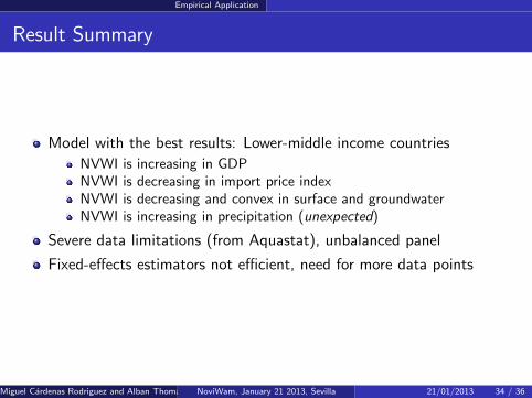
Empirical Application
Result Summary
Model with the best results: Lower-middle income countries
NVWI is increasing in GDPNVWI is decreasing in import price indexNVWI is decreasing and convex in surface and groundwaterNVWI is increasing in precipitation (unexpected)
Severe data limitations (from Aquastat), unbalanced panel
Fixed-effects estimators not efficient, need for more data points
Miguel Cardenas Rodriguez and Alban Thomas ( OECD, Paris Toulouse School of Economics (LERNA, INRA))NoviWam, January 21 2013, Sevilla 21/01/2013 34 / 36
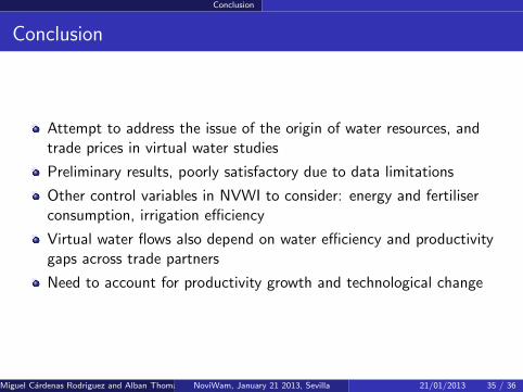
Conclusion
Conclusion
Attempt to address the issue of the origin of water resources, andtrade prices in virtual water studies
Preliminary results, poorly satisfactory due to data limitations
Other control variables in NVWI to consider: energy and fertiliserconsumption, irrigation efficiency
Virtual water flows also depend on water efficiency and productivitygaps across trade partners
Need to account for productivity growth and technological change
Miguel Cardenas Rodriguez and Alban Thomas ( OECD, Paris Toulouse School of Economics (LERNA, INRA))NoviWam, January 21 2013, Sevilla 21/01/2013 35 / 36
Conclusion
Thank you for your attention
Miguel Cardenas Rodriguez and Alban Thomas ( OECD, Paris Toulouse School of Economics (LERNA, INRA))NoviWam, January 21 2013, Sevilla 21/01/2013 36 / 36