virtual impedance techniques for power sharing control in
TRANSCRIPT
Virtual Impedance Techniques for PowerSharing Control in AC IslandedMicrogrids
Anders Bergheim Holvik
Master of Energy and Environmental Engineering
Supervisor: Ole-Morten Midtgård, IELCo-supervisor: Raymundo E. Torres-Olguin, SINTEF Energi
Department of Electric Power Engineering
Submission date: June 2018
Norwegian University of Science and Technology


Problem Description
This project will focus on developing power sharing control techniques
for ac microgrids with multiple distributed generation units. The power-
sharing within these generation units will be studied when the microgrid is
operating in island mode. In order to provide improved power sharing in
such a grid, the use of virtual impedance will be explored using a decen-
tralized approach. The performance will be assessed through simulations.
i

Abstract
This thesis focuses on power sharing in low-voltage, islanded ac micro-
grids. It is motivated by the challenges related to climate change. To
achieve a successful integration of renewable energy resources in the power
grid, it is likely with an increased use of small distributed generation units.
A promising way of organizing these units is by the use of microgrids. With
microgrids disconnected from the main grid, several challenges related to
current, voltage and power flow control arise. These challenges are studied
in this thesis, where a microgrid with two distributed generation units and
one load is investigated while operating in island mode. The two distributed
generation units in the system are implemented with significantly different
output impedances, in order to examine the unequal power distribution.
Distributed control systems are developed for this system, especially fo-
cusing on the use of virtual impedances for improved power sharing. Pro-
posed virtual impedance methods are presented. These methods reduce the
effect the virtual impedances have on the voltage level.
Three different cases are considered, each of which divided into two
subcases. In case 1, the microgrid system is assumed to have predominantly
resistive output impedances. The subcases 1 a) and 1 b) consider the use of
opposite and conventional droop control algorithms for controlling the volt-
age and frequency levels. The microgrid considered in case 2 is similar to
the one in case 1, but with predominantly inductive output impedances. As
in case 1, the conventional and opposite droop control algorithms are uti-
lized in case 2 a) and 2 b), respectively. Case 3 is a reproduction of case 2,
but in the selection of virtual impedances, the physical output impedances
ii
are estimated to be 25 % lower than the actual values.
Simulation models are carried out in all of the cases by utilizing the
software MATLAB/Simulink. Each simulation case considers the use of
physical output impedance only, an existing virtual impedance method and
a proposed virtual impedance method. The proposed virtual impedance
methods show promising results in all cases, where the power sharing per-
formances are the same as for the existing methods. The voltage drops due
to the use of virtual impedances are however significantly reduced. All of
the simulation cases show a reduction of at least 90 %.
This master’s thesis is a part of the research project FME CINELDI,
and the results of this thesis are planned to be verified through laboratory
experiments.
Trondheim, June 2018
Anders Bergheim Holvik
iii

Samandrag
I denne masteroppgåva er det fokusert på vekselspenningsmikronett med
lav spenning som opererer i øydrift. Oppgåva er motivert av utfordringane
knytta til klimaendringar. For å oppnå vellukka integrasjon av fornybare
energikjelder i kraftnettet vil det vere sannsynleg med auka bruk av dis-
tribuerte generatorar. Ein lovande måte å organisere desse enhetane er
ved bruk av mikronett. Med mikronett fråkobla hovudnettet, oppstår fleire
utfordringar knytta til straum-, spenning- og effektkontroll. Denne mas-
teroppgåva tar for seg desse utfordringane, der eit mikronett med to dis-
tribuerte generatorar og ein last er undersøkt når det opererer i øydrift.
Dei to distribuerte generatorane i systemet er implementert med signifikant
forskjell i utgongsimpedans, for å kunne studere effektfordelinga mellom
dei.
Distribuerte kontrollsystem er utvikla for systemet, der det er spesielt
fokusert på bruk av virtuell impedans for å forbetre effektdeling. Foreslåtte
metodar for bruk av virtuell impedans er presentert. Desse metodane vil
redusere effekten dei virtuelle impedansane har på spenningsnivået.
Tre forskjellege tilfeller er studert, der kvart av dei er delt inn i to un-
dertilfeller. I tilfelle 1 er det anteke at mikronettet har utgongsimpedansar
dominert av resistive komponentar. I undertilfelle 1 a) og 1 b) er det sett på
bruk av omvendt- og konvensjonell droop-kontrollar for å styre spennings-
og frekvensnivå. Mikronettet i tilfelle 2 liknar på det i tilfelle 1, men med
utgongsimpedansen dominert av induktive komponentar. Slik som i til-
felle 1, er den konvensjonelle droop-kontrollalgoritmane brukt i tilfelle 2
a) og omvendte droop-kontrollalgoritmane i tilfelle 2 b). Tilfelle 3 er ein
iv

reproduksjon av tilfelle 2, men når ein velger dei virtuelle impedansane
er dei fysiske utgongsimpedansane estimert 25 % lavare enn dei faktiske
verdiane.
Simuleringsmodellane er utarbeida ved bruk av MATLAB/Simulink.
Kvart simuleringstilfelle tek for seg fysisk utgongsimpedans, ein allereie
eksisterande virtuell impedans-metode og ein foreslått virtuell impedans-
metode. Dei foreslåtte virtuell impedans-metodane visar lovande resultat i
alle tilfella. Desse metodane gjev same effektdeling som dei eksisterande
metodane. Spenningsfalla på grunn av bruken av virtuell impedans er re-
dusert signifikant. Alle simuleringstilfella viser ein reduksjon på minst
90 %.
Denne masteroppgåva er ein del av forskningsprosjektet FME CINELDI,
og resultata frå denne oppgåva er planlagt å bli verifisert gjennom labora-
torieeksperiment.
v

Preface
This thesis is the result of my final semester as a student at the Department
of Electric Power Engineering at The Norwegian University of Science and
Technology (NTNU). The study is carried out as a part of the work package
on microgrids in the research project FME CINELDI. In the work of this
master’s thesis, there are several contributors, and I would like to thank all
of you.
In particular, I would like to thank my supervisor Ole-Morten Midtgård
for guidance and making it possible to perform this master’s thesis.
My greatest gratitude goes to Fredrik Tomas Bjørndalen Wergeland
Göthner for invaluable help and discussions. His talent and pedagogical
skills have been extremely helpful throughout my year as a fifth year stu-
dent at NTNU.
I sincerely thank my co-supervisor Raymundo E. Torres-Olguin in SIN-
TEF Energy for sharing his knowledge and experience with me. He has
provided guidance in any way, and I am extremely grateful for his help.
Last, but sincerely not least, I want to thank my partner, Nora, for her
support and for helping proofreading my report.
vi

Table of Contents
Abstract ii
Samandrag iv
Preface vi
Table of Contents x
List of Tables xi
List of Figures xv
Abbreviations xvi
1 Introduction 11.1 Background and Motivation . . . . . . . . . . . . . . . . 1
1.2 Relation to Specialization Project . . . . . . . . . . . . . . 4
1.3 Objectives . . . . . . . . . . . . . . . . . . . . . . . . . . 5
1.4 Methodology and Scope . . . . . . . . . . . . . . . . . . 5
1.5 Outline . . . . . . . . . . . . . . . . . . . . . . . . . . . 6
2 System Description 72.1 Microgrid System . . . . . . . . . . . . . . . . . . . . . . 7
vii

2.2 Distributed Generation . . . . . . . . . . . . . . . . . . . 9
2.3 Low-Pass Filter . . . . . . . . . . . . . . . . . . . . . . . 9
2.3.1 Filter Resistors . . . . . . . . . . . . . . . . . . . 11
2.4 Distribution Lines . . . . . . . . . . . . . . . . . . . . . . 12
2.5 Load . . . . . . . . . . . . . . . . . . . . . . . . . . . . . 13
2.6 Voltage Source Inverter . . . . . . . . . . . . . . . . . . . 14
2.6.1 Pulse-Width Modulation . . . . . . . . . . . . . . 15
2.6.2 Average Model VSI . . . . . . . . . . . . . . . . 16
2.7 Per-Unit System . . . . . . . . . . . . . . . . . . . . . . . 18
3 Power Flow Control 213.1 Circulating Current . . . . . . . . . . . . . . . . . . . . . 21
3.2 Hierarchical Control Structure . . . . . . . . . . . . . . . 24
3.3 Inner control . . . . . . . . . . . . . . . . . . . . . . . . . 26
3.3.1 Vector Control . . . . . . . . . . . . . . . . . . . 27
3.3.2 Current Controller . . . . . . . . . . . . . . . . . 28
3.3.3 Voltage Control . . . . . . . . . . . . . . . . . . . 29
3.3.4 PI-Controllers . . . . . . . . . . . . . . . . . . . . 32
3.4 Primary Control . . . . . . . . . . . . . . . . . . . . . . . 34
3.4.1 Droop Control . . . . . . . . . . . . . . . . . . . 35
3.4.2 Mixed Output Impedance . . . . . . . . . . . . . 44
3.4.3 Virtual Impedance . . . . . . . . . . . . . . . . . 46
4 Cases Studies 554.1 General Parameters . . . . . . . . . . . . . . . . . . . . . 56
4.2 Case 1: Resistive Output Impedance . . . . . . . . . . . . 58
4.2.1 Case 1 a): Opposite Droop Control . . . . . . . . 59
4.2.2 Case 1 b): Conventional Droop Control . . . . . . 62
4.3 Case 2: Inductive Output Impedance . . . . . . . . . . . . 67
4.3.1 Case 2 a): Conventional Droop Control . . . . . . 68
viii

4.3.2 Case 2 b): Opposite Droop Control . . . . . . . . 72
4.4 Case 3: Estimated Inductive Output Impedance . . . . . . 76
4.4.1 Case 3 a): Conventional Droop Control . . . . . . 76
4.4.2 Case 3 b): Opposite Droop Control . . . . . . . . 80
4.5 Discussion . . . . . . . . . . . . . . . . . . . . . . . . . . 83
5 Conclusion 89
Bibliography 90
Appendix A Park Transform 103
Appendix B Transfer Functions for Low-Pass Filters 105
Appendix C Matlab-Code for Bode Plots of LCL-Filters 107
Appendix D Additional Simulation Parameters 111
Appendix E Tuning of PI-Controllers 113E.1 Current Control . . . . . . . . . . . . . . . . . . . . . . . 113
E.2 Voltage Control . . . . . . . . . . . . . . . . . . . . . . . 114
Appendix F Bode Plots of Current- and Voltage Controllers 115
Appendix G MATLAB-Code for Bode-Plots of Current- and Volt-age Controllers 117
Appendix H Response of the Controllers 123
Appendix I Simulink Models 129I.1 Microgrid Model . . . . . . . . . . . . . . . . . . . . . . 129
I.2 Current Controller . . . . . . . . . . . . . . . . . . . . . . 130
I.3 Voltage Controller . . . . . . . . . . . . . . . . . . . . . . 131
ix

I.4 Conventional Droop Controller . . . . . . . . . . . . . . . 132
I.5 Opposite Droop Controller . . . . . . . . . . . . . . . . . 133
I.6 Virtual Impedance . . . . . . . . . . . . . . . . . . . . . . 134
Appendix J Chapter 2 from "Control of Power Electronics in Mi-crogrids" 135
x
List of Tables
2.1 Parameters of the LCL-filters available in the Smart Grid
Laboratory . . . . . . . . . . . . . . . . . . . . . . . . . . 11
2.2 Typical line parameters for different voltage levels [1] . . . 13
4.1 General parameters . . . . . . . . . . . . . . . . . . . . . 56
4.2 Control parameters . . . . . . . . . . . . . . . . . . . . . 57
4.3 Physical output impedances for the resistive-dominating mi-
crogrid used in case 1 . . . . . . . . . . . . . . . . . . . . 59
4.4 Virtual resistance and inductance used in case 1 a) . . . . . 60
4.5 Virtual resistance and inductance used in case 1 b) . . . . . 63
4.6 Physical output impedances used in the inductive-dominating
microgrid in case 2 and case 3 . . . . . . . . . . . . . . . 68
4.7 Virtual resistance and inductance used in case 2 a) . . . . . 69
4.8 Virtual resistance and inductance used in case 2 b) . . . . . 72
4.9 Virtual resistance and inductance used in case 3 a) . . . . . 77
4.10 Virtual resistance and inductance used in case 3 b) . . . . . 80
D.1 Parameters used to develop simulation parameters in the
case studies . . . . . . . . . . . . . . . . . . . . . . . . . 111
D.2 Base values used in the per-unit representation . . . . . . . 112
xi

xii
List of Figures
2.1 The investigated system . . . . . . . . . . . . . . . . . . . 8
2.2 Bode plots for three different low-pass filter alternatives . . 10
2.3 Schematic of a low-pass LCL-filter . . . . . . . . . . . . . 11
2.4 Bode plots for LCL with internal resistors included and
omitted . . . . . . . . . . . . . . . . . . . . . . . . . . . 12
2.5 Representation of a voltage source inverter . . . . . . . . . 15
2.6 Pulse-width modulation . . . . . . . . . . . . . . . . . . . 16
2.7 Schematic showing a three-phase average model VSI . . . 17
2.8 The output voltage from an average model and switching
model VSI . . . . . . . . . . . . . . . . . . . . . . . . . 18
3.1 Two inverters with different line impedance, delivering power
to the same load . . . . . . . . . . . . . . . . . . . . . . . 22
3.2 Active and reactive component of circulating currents . . . 23
3.3 Hierarchircal control structure . . . . . . . . . . . . . . . 25
3.4 The cascaded control loop . . . . . . . . . . . . . . . . . 27
3.5 Three-phase inverter . . . . . . . . . . . . . . . . . . . . 28
3.6 Block diagrams showing the current controller . . . . . . . 30
3.7 Block diagrams showing the voltage controller . . . . . . 32
3.8 General block diagram for the approach for the inner con-
trollers . . . . . . . . . . . . . . . . . . . . . . . . . . . . 33
xiii

3.9 A representation of power flow through a distribution line . 36
3.10 The characteristic of the conventional droop control . . . . 38
3.11 Implementation of the conventional droop control method . 41
3.12 The characteristic of the opposite droop control . . . . . . 42
3.13 Implementation of the opposite droop control method . . . 44
3.14 Block diagram showing an outer virtual impedance loop . 47
3.15 Schematic of the implementation of virtual impedance . . 53
4.1 The investigated system in case 1 . . . . . . . . . . . . . . 58
4.2 Power Flows with predominantly resistive physical impedance
and opposite droop control . . . . . . . . . . . . . . . . . 61
4.3 Output voltage with predominantly resistive physical impedance
and opposite droop control . . . . . . . . . . . . . . . . . 62
4.4 Power flows in the first simulation with predominantly re-
sistive physical impedance and opposite droop control . . . 64
4.5 Power flows in the second simulation with predominantly
resistive physical impedance and opposite droop control . 65
4.6 Output voltage in the second simulation with predominantly
resistive physical impedance and opposite droop control . 66
4.7 The investigated system in case 2 . . . . . . . . . . . . . . 67
4.8 Power flows with predominantly inductive physical impedance
and conventional droop control . . . . . . . . . . . . . . . 70
4.9 The output voltage with predominantly inductive physical
impedance and conventional droop control . . . . . . . . . 71
4.10 Active and reactive power in first simulation with predom-
inantly inductive physical impedance and opposite droop
control . . . . . . . . . . . . . . . . . . . . . . . . . . . . 73
4.11 Power flows in second simulation with predominantly in-
ductive physical impedance and opposite droop control . . 74
xiv

4.12 Output voltage in second simulation with predominantly
inductive physical impedance and opposite droop control . 75
4.13 Power flows in second simulation with estimated predomi-
nantly inductive physical impedance and conventional droop
control . . . . . . . . . . . . . . . . . . . . . . . . . . . . 78
4.14 Output voltage with estimated inductive physical impedance
and conventional droop control . . . . . . . . . . . . . . . 79
4.15 Power flows with estimated predominantly inductive phys-
ical impedance and opposite droop control . . . . . . . . . 81
4.16 Output voltage with estimated inductive physical impedance
and opposite droop control . . . . . . . . . . . . . . . . . 82
4.17 A representation of a laboratory setup for a microgrid. Used
by permission of FME CINELDI. . . . . . . . . . . . . . 87
A.1 The synchronous reference frame with frequency ω . . . . 104
F.1 Bode plot of the open current loop . . . . . . . . . . . . . 115
F.2 Bode plot of the open voltage loop . . . . . . . . . . . . . 116
H.1 Response of the conventional droop controller . . . . . . . 124
H.2 Response of the opposite droop controller . . . . . . . . . 125
H.3 Response of the voltage controller . . . . . . . . . . . . . 126
H.4 Response of the current controller . . . . . . . . . . . . . 127
xv
Abbreviations
ac Alternating Current
RES Renewable Energy Sources
PV Photovoltaic
DG Distributed Generation
IEA The International Energy Agency
DER Distributed Energy Resources
dc Direct Current
VSI Voltage Source Inverter
PWM Pulse Width Modulation
pu Per-unit
xvi
1 | Introduction
1.1 Background and Motivation
By March 2018, 195 countries have signed the Paris Agreement [2], due to
the large concern climate change is posing worldwide. Thereby, they have
commited to contribute to limit the global temperature rise to 2 degrees
Celsius [3]. With an increasing global population [4], the world’s electricity
production has to be changed to a larger extent renewable energy sources
(RES) if this goal should be seen as realistic [5].
Promising technologies to contribute to increased use of RES are sys-
tems based on resources such as solar, wind, hydro, and biomass [6]. These
technologies have received much attention in the global society, which can
be shown by the increase in total production from PV-systems and wind-
turbines. From 2005 to 2015, the production of these technologies was
increased by a multiple of 10 [7].
In order to increase the capacity and perform a successful integration of
RES in the power grid, an increased use of small-scale generation units is
expected [8]. These will be distributed at different locations in the power
grid, referred to as distributed generation (DG) [9, chapter 1]. The use of
RES will make the need of power electronic interfaces in the distributed
generation units significant [10]. The intermittent behavior of RES will
lead to increased challenges for the power system. To increase the power
1
Chapter 1. Introduction
capacity of a grid, these units can be connected in parallel. This brings new
challenges related to the power delivery and stability [11].
The traditional power grid is dominated by unidirectional power flows
and production mainly based on large synchronous generators. The de-
velopment towards more renewable generation leads to, in addition to the
already mentioned distributed generation, new aspects such as energy stor-
age units located in the grid. This leads to bidirectional power flows, having
customers who both consume and produce energy. These are referred in the
literature as prosumers [12].
Because of the current evolution within DG, the traditional control tech-
niques based on large, synchronous generators are not necessarily valid in
the future power grid [9, chapter 1]. New control techniques have to be
developed, which should both meet the new challenges and comply with
the advantages related to upcoming technologies and generation units with
power electronic interfaces.
The challenges related to the integration of RES can be faced through
the approach of a small version of a power system which contains dis-
tributed generation and energy storage, referred in the literature as micro-
grids. The definition of a microgrid includes that it has clearly defined elec-
trical boundaries, local control systems and flexible loads [9, chapter 1].
This can be advantageous for the purpose of integrating DG, secure power
supply and meeting challenges related to bidirectional power flows, pro-
sumers and intermittent generation [9, chapter 1]. Microgrids can operate
connected to the main grid, but also as isolated grids. The latter mode of
operation is frequently referred to as "island mode", and requires some kind
of energy storage and local control systems.
In the island mode of operation, control of power flow, voltage and
frequency are essential. Each generation unit will include a local control
system, which is responsible for the voltage and frequency levels in the mi-
2
1.1 Background and Motivation
crogrid. This mode of operation can contribute to secure the power supply
in case of unintended disconnection from the main grid [9, chapter 1]. It
can also contribute to secure the power supply in rural areas without con-
nection to the main grid. According to The International Energy Agency
(IEA), 70 % of rural areas without electricity access have to connect to
off-grid solutions or mini-grids in order to achieve this access in the future
[13]. In the small grids established in these areas, the research on islanded
microgrids can be beneficial.
When connected to the grid, microgrids are seen as single units by the
main grid, because of their local control systems [14]. The voltage level
is normally stabilized due to the main grid, which makes the main control
task related to the power supplied from the DG units [15].
The local control system of a microgrid can be utilized by using either a
centralized or a decentralized control approach. In a centralized approach,
the control systems located at the DG units follow commands from the mi-
crogrid’s central controller [16]. When utilizing this approach, the central
controller can control the different units relative to each other. Compared
to a decentralized approach, power flow control and safe operation of the
microgrid are simplified [6] [17]. The centralized approach also brings
challenges, for instance by the high costs related to the need of communi-
cation [9, chapter 1]. The centralized controller is designed for a specific
microgrid, which makes it more challenging if the microgrid is expanded
with additional units or in case of a DG failure [18]. With the microgrid
dependent on the centralized controller, a failure related to the control or its
communication can break down the whole microgrid operation.
A microgrid controlled through a decentralized approach has more in-
telligent controllers located at the DG units compared to a microgrid con-
trolled by a centralized approach[16]. The decentralized control has more
challenges related to the interaction between the DG units, including power
3
Chapter 1. Introduction
flow issues [18] [16], since the control is done locally. With local measure-
ments, this control approach is more reliable when it comes to DG failure
or in case of expansions of the microgrid. Because of these advantages, this
thesis will focus on the decentralized control approach. This approach has
the intention of making a more general study since the controllers are not
dependent on a specific microgrid system. Even if the decentralized con-
trollers are less dependent on communication, it is worth to mention that
they are not totally communication-less. The communication is related to
the higher levels of control, which operates at a relatively slow sampling
rate. The consequences of issues related to this communication will, there-
fore, be smaller than in case of a centralized controller. In this thesis, the
high level control is outside of the scope.
The distributed control, located at the DG units, will be the primary
focus of this work. The microgrid studied will be operating in island mode,
where power flow challenges will be studied in detail, developing control
systems for the purpose of a well-functional islanded microgrid. The results
of this thesis will form the foundation for future laboratory experiments
utilized through the research project FME CINELDI.
1.2 Relation to Specialization Project
In the fall of 2017, the author wrote a specialization project entitled "Con-
trol of Power Electronics in Microgrids" [19]. Some sections in this thesis
contain material reused from the specialization project, where most of the
material is modified. The relevant chapter from the specialization project is
given in App. J. The sections which include some reused material are:
• Section 2.6 about the voltage source inverter.
• Section 3.4.1 about different droop control algorithms.
• Section 3.4.3 about virtual impedance.
4

1.3 Objectives
• Section 3.1 about circulating currents.
• Section 3.2 about the hierarchical control structure.
• Section A about the park transform.
1.3 Objectives
The general objective of this master thesis is to:
• Investigate control of power sharing in low-voltage islanded ac mi-
crogrids with linear loads.
In particular, the following objectives have been considered:
• Develop a distributed control system for paralleled DG units operat-
ing in an islanded microgrid.
• Investigate how virtual impedance can be used with droop control
algorithms to improve power sharing.
• Examine the concepts through a developed microgrid system in MAT-
LAB/Simulink.
1.4 Methodology and Scope
In order to achieve the aforementioned objectives, this thesis will study the
local control systems in a three-phase islanded ac microgrid. It considers
a decentralized control approach, focusing on the distributed control. The
higher levels of control are assumed to be ideal i.e. the controllers provide
constant references to the inner controllers under study.
The microgrid investigated is loaded with a single linear load, modelled
as a constant impedance. Neither harmonic oscillations or losses related
to the inverters are taken into consideration. The system is assumed to be
5
Chapter 1. Introduction
balanced, and it is focused on the steady-state behavior. Two DG units
are considered in the microgrid, and these are modelled as ideal dc voltage
sources. To study the power sharing performance, the impedances of the
distribution lines connected to the DGs are significantly different. The goal
is to make the two DG units equally share the power drawn from the load.
The microgrid system is modelled in MATLAB/Simulink, where local
control systems for the inverters connected to the two DGs are developed.
This includes current and voltage control. Active and reactive power are
controlled by regulating the voltage and frequency. This is utilized through
droop control algorithms and the use of virtual impedances.
1.5 Outline
This section presents the outline of the thesis.
Chapter 2 presents the microgrid system used in this thesis. Some of
the microgrid’s fundamental components are explained, in addition to im-
portant definitions.
In chapter 3, it is elaborated on power flow control in microgrids. Defi-
nitions, including common control structures, are explained before the con-
trol systems utilized in this thesis are studied in detail. In this chapter,
concepts such as droop control and the use of virtual impedance are in-
troduced. Both already existing virtual impedance methods and proposed
solutions will be elaborated on.
Chapter 4 presents the case studies utilized through this work. Six dif-
ferent cases are considered, where the use of droop control and virtual
impedances are the primary focus. This chapter is summarized with a dis-
cussion of the results, related to the theory presented in chapter 3.
Finally, chapter 5 provides the final remarks in the thesis.
6
2 | System Description
In order to study the control of power sharing in ac microgrids and ex-
amine control concepts, a specific microgrid system is used. This chapter
will present the system, including some of its most important components.
Lastly, the per-unit system used in this thesis will be presented in this chap-
ter.
2.1 Microgrid System
Microgrids exist in many forms, in terms of distributed energy resources
(DERs), loads, and topology. The complexity and behavior are dependent
on the number of loads and DERs, in addition to their characteristics. This
study will aim for a generalization, and the conclusions drawn can there-
fore indicate consequences in other microgrids. The investigated system is
chosen on the basis of this generalization.
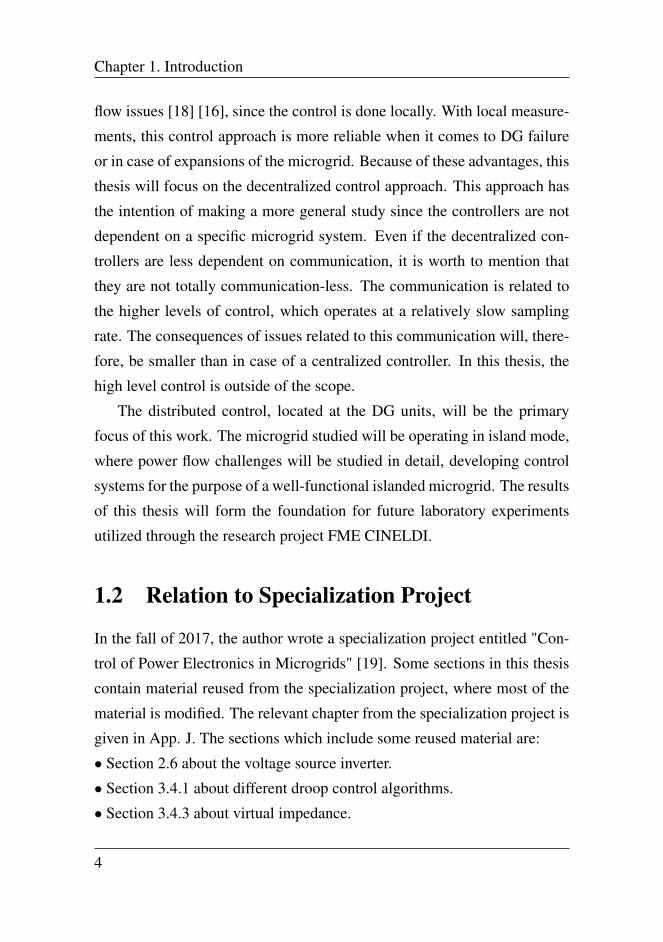
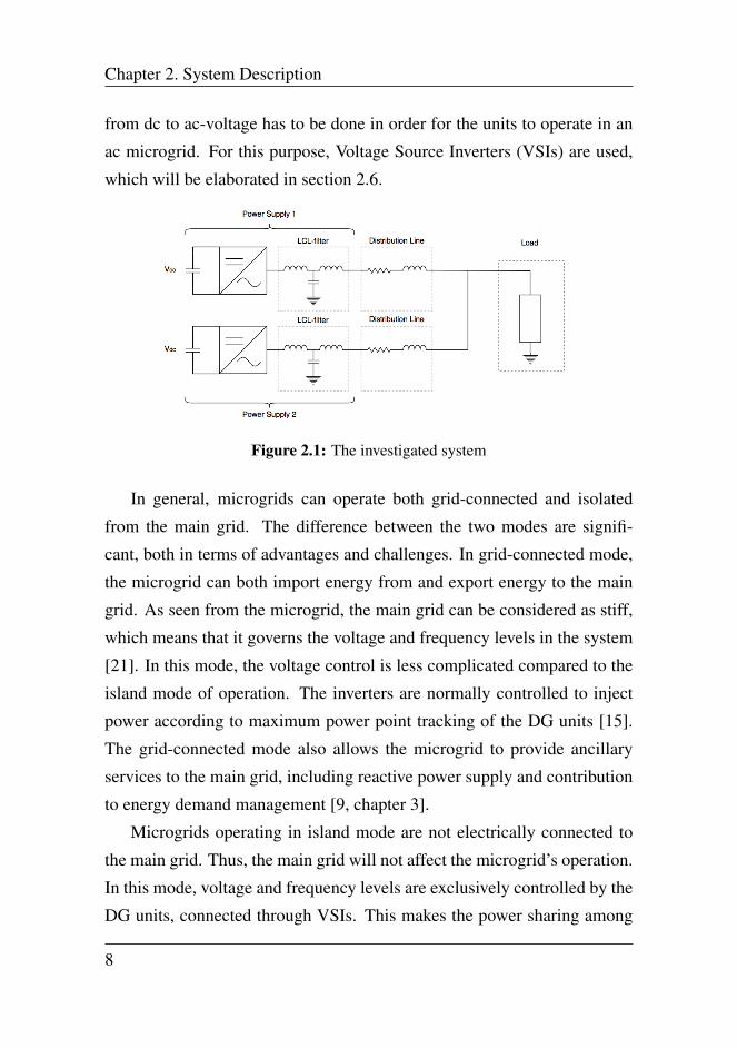
The system examined in this thesis is depicted in Fig. 2.1. As shown
in the figure, the microgrid includes one residential load, represented as a
linear, resistive-inductive component. In order to secure reasonable values
for the system, a microgrid benchmark presented in [20] is used.
The microgrid has two DG units, where each of them is connected to an
LCL-filter in order to reduce harmonic oscillations. Both of the DG units
are modelled as ideal dc voltage sources, which means that a conversion
7
Chapter 2. System Description
from dc to ac-voltage has to be done in order for the units to operate in an
ac microgrid. For this purpose, Voltage Source Inverters (VSIs) are used,
which will be elaborated in section 2.6.
Figure 2.1: The investigated system
In general, microgrids can operate both grid-connected and isolated
from the main grid. The difference between the two modes are signifi-
cant, both in terms of advantages and challenges. In grid-connected mode,
the microgrid can both import energy from and export energy to the main
grid. As seen from the microgrid, the main grid can be considered as stiff,
which means that it governs the voltage and frequency levels in the system
[21]. In this mode, the voltage control is less complicated compared to the
island mode of operation. The inverters are normally controlled to inject
power according to maximum power point tracking of the DG units [15].
The grid-connected mode also allows the microgrid to provide ancillary
services to the main grid, including reactive power supply and contribution
to energy demand management [9, chapter 3].
Microgrids operating in island mode are not electrically connected to
the main grid. Thus, the main grid will not affect the microgrid’s operation.
In this mode, voltage and frequency levels are exclusively controlled by the
DG units, connected through VSIs. This makes the power sharing among
8

2.2 Distributed Generation
several DG units challenging in an isolated microgrid, for instance, due to
a difference in line impedances, different voltage levels or local loads [22].
Challenges related to power sharing will be the primary focus throughout
this thesis. The microgrid in Fig. 2.1 will be the investigated system, used
to highlight both challenges and solutions. Circulating currents and power
sharing issues while operating in island mode will be the main concern,
focusing on control techniques to solve issues related to this.
In the following, components and definitions that play a central role in
this thesis will be introduced, beginning with the distributed generation.
2.2 Distributed Generation
The main objective of this thesis is to study the power sharing among the
inverters connected to the DG units in the microgrid system. The DG units
are modelled as ideal dc voltage sources. This modelling does not take
the size of these units, neither in terms of power or storage capacity into
consideration. Both inverters are assumed to produce the required amount
of power at any time, where the goal is to make the two inverters equally
share the load drawn from the load.
2.3 Low-Pass Filter
In order to filter high-frequency harmonics, low-pass filters are located at
the inverters’ output. When selecting this kind of filter, there are several
options. The harmonics can be filtered through a simple inductor, referred
to as an L-filter. Two other common alternatives are LC- or LCL-filters,
both designed by a combination of inductors and capacitors [23].
The low-pass filters selected for this work are LCL-filters, which of the
alternatives is the cheaper since the inductors can be smaller than when us-
9
Chapter 2. System Description
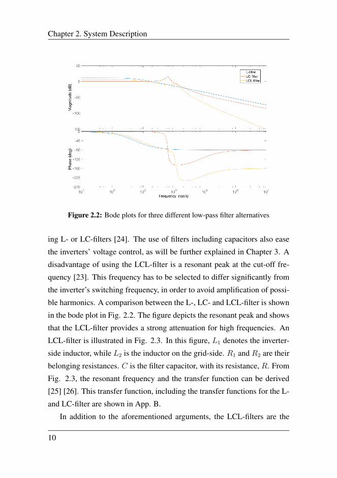
Figure 2.2: Bode plots for three different low-pass filter alternatives
ing L- or LC-filters [24]. The use of filters including capacitors also ease
the inverters’ voltage control, as will be further explained in Chapter 3. A
disadvantage of using the LCL-filter is a resonant peak at the cut-off fre-
quency [23]. This frequency has to be selected to differ significantly from
the inverter’s switching frequency, in order to avoid amplification of possi-
ble harmonics. A comparison between the L-, LC- and LCL-filter is shown
in the bode plot in Fig. 2.2. The figure depicts the resonant peak and shows
that the LCL-filter provides a strong attenuation for high frequencies. An
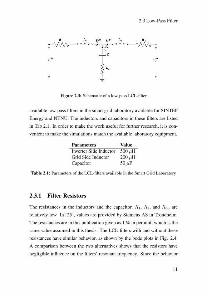
LCL-filter is illustrated in Fig. 2.3. In this figure, L1 denotes the inverter-
side inductor, while L2 is the inductor on the grid-side. R1 and R2 are their
belonging resistances. C is the filter capacitor, with its resistance, R. From
Fig. 2.3, the resonant frequency and the transfer function can be derived
[25] [26]. This transfer function, including the transfer functions for the L-
and LC-filter are shown in App. B.
In addition to the aforementioned arguments, the LCL-filters are the
10
2.3 Low-Pass Filter
Figure 2.3: Schematic of a low-pass LCL-filter
available low-pass filters in the smart grid laboratory available for SINTEF
Energy and NTNU. The inductors and capacitors in these filters are listed
in Tab 2.1. In order to make the work useful for further research, it is con-
venient to make the simulations match the available laboratory equipment.
Parameters ValueInverter Side Inductor 500 µHGrid Side Inductor 200 µHCapacitor 50 µF
Table 2.1: Parameters of the LCL-filters available in the Smart Grid Laboratory
2.3.1 Filter Resistors
The resistances in the inductors and the capacitor, R1, R2, and RC , are
relatively low. In [25], values are provided by Siemens AS in Trondheim.
The resistances are in this publication given as 1 % in per unit, which is the
same value assumed in this thesis. The LCL-filters with and without these
resistances have similar behavior, as shown by the bode plots in Fig. 2.4.
A comparison between the two alternatives shows that the resistors have
negligible influence on the filters’ resonant frequency. Since the behavior
11

Chapter 2. System Description
Figure 2.4: Bode plots for LCL with internal resistors included and omitted
of the filters is similar without the resistors, R2 and RC are omitted in this
work’s analyses. A small inverter-side resistor is however included since
this is used to select parameters for the inner controllers in Section 3.3.
The bode plots are given in Fig. 2.2 and 2.4 are provided by the MATLAB
script given in App. C.
2.4 Distribution Lines
The distribution lines in a grid are dependent on the voltage level used
for power transfer. This work focuses on a low-voltage microgrid, and as
shown in Tab. 2.2 [1], these feeders will typically be dominated by the
resistive components.
As will be further explained in Section 3.4.1, the power sharing con-
trol techniques used in this work are highly affected by the values of the
line impedances, in addition to possible components located between the
12
2.5 Load
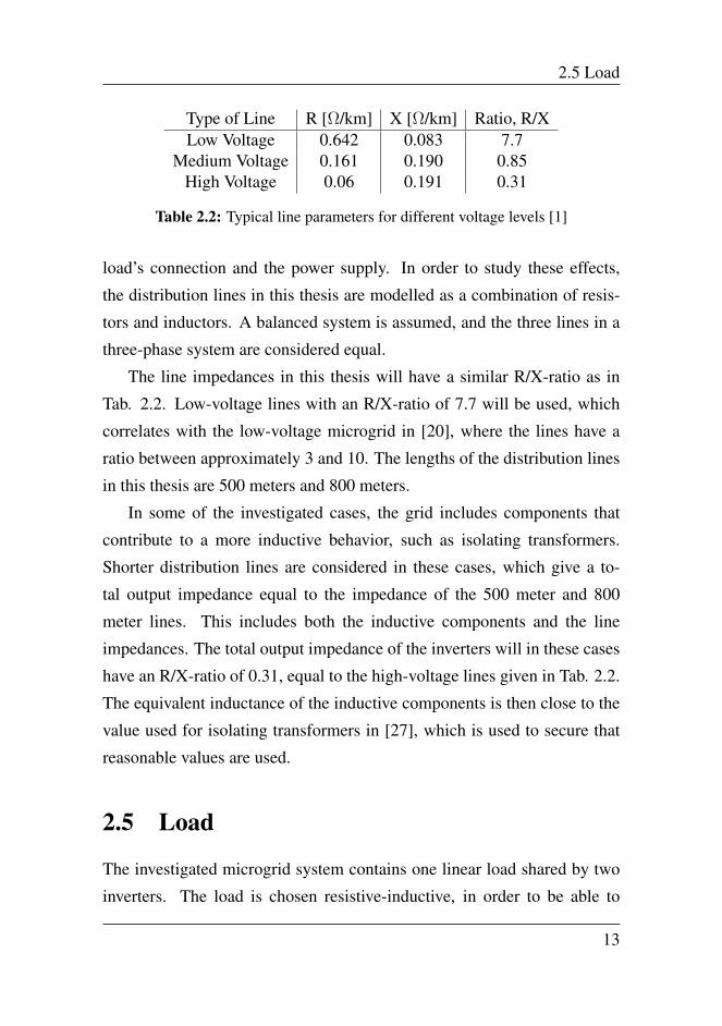
Type of Line R [Ω/km] X [Ω/km] Ratio, R/XLow Voltage 0.642 0.083 7.7
Medium Voltage 0.161 0.190 0.85High Voltage 0.06 0.191 0.31
Table 2.2: Typical line parameters for different voltage levels [1]
load’s connection and the power supply. In order to study these effects,
the distribution lines in this thesis are modelled as a combination of resis-
tors and inductors. A balanced system is assumed, and the three lines in a
three-phase system are considered equal.
The line impedances in this thesis will have a similar R/X-ratio as in
Tab. 2.2. Low-voltage lines with an R/X-ratio of 7.7 will be used, which
correlates with the low-voltage microgrid in [20], where the lines have a
ratio between approximately 3 and 10. The lengths of the distribution lines
in this thesis are 500 meters and 800 meters.
In some of the investigated cases, the grid includes components that
contribute to a more inductive behavior, such as isolating transformers.
Shorter distribution lines are considered in these cases, which give a to-
tal output impedance equal to the impedance of the 500 meter and 800
meter lines. This includes both the inductive components and the line
impedances. The total output impedance of the inverters will in these cases
have an R/X-ratio of 0.31, equal to the high-voltage lines given in Tab. 2.2.
The equivalent inductance of the inductive components is then close to the
value used for isolating transformers in [27], which is used to secure that
reasonable values are used.
2.5 Load
The investigated microgrid system contains one linear load shared by two
inverters. The load is chosen resistive-inductive, in order to be able to
13
Chapter 2. System Description
study both the active and reactive power flow. It is modelled as a constant
impedance, adjusted to extract the nominal power at the nominal voltage.
By (2.1), it is evident that a reduced voltage level will lead to a decreased
power to the load. In this equation, VLL is the amplitude of the voltage
across the load, while Z is the load’s impedance. The load’s apparent power
is denoted as S.
S =V 2LL
Z(2.1)
The size of the load is chosen to model a residential load, as given in
the benchmark microgrid [20]. The load consists of both a resistive and an
inductive component, which is convenient in order to study both the active
and reactive power sharing.
2.6 Voltage Source Inverter
A VSI is used to convert the dc-voltage to ac-voltage by using semicon-
ducting switches. Since the DG units are based on dc-voltages, the VSIs
are central in the operation of the microgrid under study. The local con-
trol of the microgrid is also done through a control system for each VSI. A
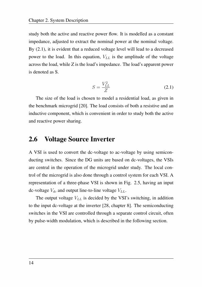
representation of a three-phase VSI is shown in Fig. 2.5, having an input
dc-voltage Vdc and output line-to-line voltage VLL.
The output voltage VLL is decided by the VSI’s switching, in addition
to the input dc-voltage at the inverter [28, chapter 8]. The semiconducting
switches in the VSI are controlled through a separate control circuit, often
by pulse-width modulation, which is described in the following section.
14

2.6 Voltage Source Inverter
Figure 2.5: Representation of a voltage source inverter
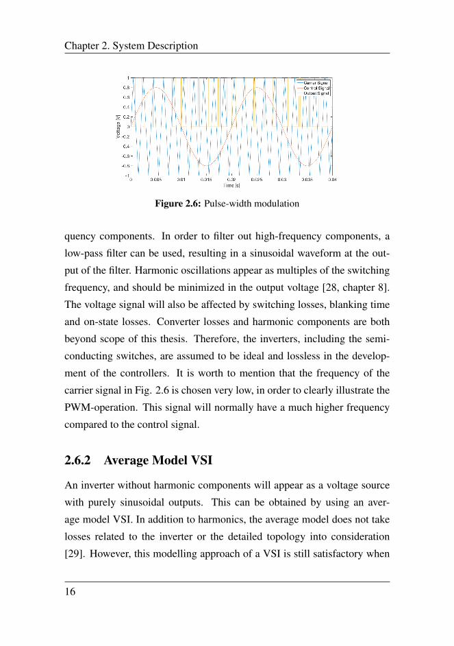
2.6.1 Pulse-Width Modulation
To control the VSI’s semiconducting switches, the sinusoidal pulse-width
modulation (PWM) technique is frequently used. The method uses a volt-
age control signal, vcontrol, in comparison with a high-frequency triangular
waveform. This is denoted vtri, and is often called the carrier signal. The
control signal represents the reference output voltage, and typically has an
amplitude of 80 % of the triangular wave [28, chapter 8].
A PWM-scheme for phase a in a three-phase system is shown in Fig.
2.6. With Fig. 2.5 as a basis, the switch Ta+ conducts if vcontrol > vtri,
while it is open when vtri > vcontrol. This results in an output phase voltage
as shown in the Fig. 2.6. The switching frequency of the semiconducting
switches is equal to the frequency of the carrier signal [28, chapter 8]. The
control signals of the three phases are 120 shifted, where all of the phases
are compared to the same triangular wave. The three phases are by this
method controlled independently of each other [28, chapter 8].
The output voltage in Fig. 2.6 is a sinusoidal wave including high fre-
15
Chapter 2. System Description
Figure 2.6: Pulse-width modulation
quency components. In order to filter out high-frequency components, a
low-pass filter can be used, resulting in a sinusoidal waveform at the out-
put of the filter. Harmonic oscillations appear as multiples of the switching
frequency, and should be minimized in the output voltage [28, chapter 8].
The voltage signal will also be affected by switching losses, blanking time
and on-state losses. Converter losses and harmonic components are both
beyond scope of this thesis. Therefore, the inverters, including the semi-
conducting switches, are assumed to be ideal and lossless in the develop-
ment of the controllers. It is worth to mention that the frequency of the
carrier signal in Fig. 2.6 is chosen very low, in order to clearly illustrate the
PWM-operation. This signal will normally have a much higher frequency
compared to the control signal.
2.6.2 Average Model VSI
An inverter without harmonic components will appear as a voltage source
with purely sinusoidal outputs. This can be obtained by using an aver-
age model VSI. In addition to harmonics, the average model does not take
losses related to the inverter or the detailed topology into consideration
[29]. However, this modelling approach of a VSI is still satisfactory when
16
2.6 Voltage Source Inverter
the phenomena studied are related to the fundamental frequency. Because
of the simplifications done when using the average model, simulations can
be performed with a larger step size compared to the PWM. Therefore, the
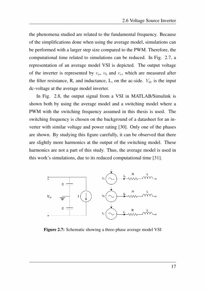
computational time related to simulations can be reduced. In Fig. 2.7, a
representation of an average model VSI is depicted. The output voltage
of the inverter is represented by va, vb and vc, which are measured after
the filter resistance, R, and inductance, L, on the ac-side. Vdc is the input
dc-voltage at the average model inverter.
In Fig. 2.8, the output signal from a VSI in MATLAB/Simulink is
shown both by using the average model and a switching model where a
PWM with the switching frequency assumed in this thesis is used. The
switching frequency is chosen on the background of a datasheet for an in-
verter with similar voltage and power rating [30]. Only one of the phases
are shown. By studying this figure carefully, it can be observed that there
are slightly more harmonics at the output of the switching model. These
harmonics are not a part of this study. Thus, the average model is used in
this work’s simulations, due to its reduced computational time [31].
Figure 2.7: Schematic showing a three-phase average model VSI
17

Chapter 2. System Description
(a) Average model (b) Switching Model
Figure 2.8: The output voltage from an average model and switching model VSI
2.7 Per-Unit System
In order to simplify calculations and utilize a generalization, the per-unit
(pu) system is used in the representation of the physical quantities. These
pu-values are given by a set of base-values, defined in (2.2) to (2.6). The
nominal line-to-line voltage, current and frequency are denoted by Vn, Inand fn. The subscript base denotes base values, where V, I, S and ω denote
voltage, current, apparent power and frequency.
Vbase =
√2√3Vn (2.2)
Ibase =√
2In (2.3)
Sbase =3
2VbaseIbase (2.4)
18
2.7 Per-Unit System
Zbase =VbaseIbase
(2.5)
ωbase = 2πfn (2.6)
The base values for inductance and capacitance are then given by (2.7)
and (2.8).
Lbase = ωbaseZbase (2.7)
Cbase =1
ωbaseZbase(2.8)
The use of the pu-system is of particular interest in the microgrid’s con-
trol system. The following chapter will elaborate on control of islanded
microgrids, focusing on power sharing challenges in particular.
19

Chapter 2. System Description
20

3 | Power Flow Control
In order to be able to develop power sharing control techniques, challenges
and solutions related to the topic will be presented in this chapter. First,
circulating currents will be defined and discussed. Subsequently, the con-
trol structure used in this work will be presented, including a more detailed
explanation regarding each control level. This includes voltage and fre-
quency control, droop control techniques and elaboration on how virtual
impedances can be used to improve the power sharing performance.
3.1 Circulating Current
The use of paralleled inverters is advantageous when it comes to increased
reliability and power rating, and is also one of the characteristics of islanded
microgrids [11]. However, this organization of DG units also brings chal-
lenges. The generation of circulating currents is one of these, which will be
presented in this section.
DG units operating in parallel with different output voltages, output
impedance or phase can cause currents not only flowing from the gener-
ation to the loads but also between the generation units. These currents
are referred to as circulating currents, and can be large and potentially
damaging. In a traditional power grid with large synchronous generators,
the line impedances normally reduce these currents, while the smaller line
21
Chapter 3. Power Flow Control
impedances in microgrids make the circulating currents a major challenge
[14].
The circulating currents can lead to increased losses and overloaded in-
verters, in addition to reductions in power quality and efficiency [32]. Since
the voltages in islanded microgrids are set by the paralleled inverters with-
out a stiff grid, the challenges related to circulating currents are of particular
interest in this mode of operation [14]. As mentioned in Chapter 1, a de-
centralized control approach has more issues related to circulating currents
than a centralized controller, where there are fewer challenges related to the
interaction between the inverters [18] [16].
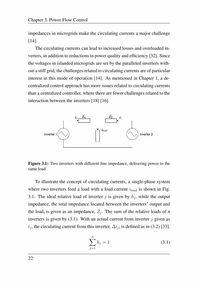
Figure 3.1: Two inverters with different line impedance, delivering power to thesame load
To illustrate the concept of circulating currents, a single-phase system
where two inverters feed a load with a load current iload is shown in Fig.
3.1. The ideal relative load of inverter j is given by hj , while the output
impedance, the total impedance located between the inverters’ output and
the load, is given as an impedance, Zj . The sum of the relative loads of n
inverters is given by (3.1). With an actual current from inverter j given as
ij , the circulating current from this inverter, ∆ij , is defined as in (3.2) [33].
n∑
j=1
hj = 1 (3.1)
22
3.1 Circulating Current
∆ij = ij − hj · iload (3.2)
Ideally, (3.1) and (3.2) show that the circulating currents of all inverters
are zero. A case where the two inverters in Fig. 3.1 are meant to share the
load equally can, for instance, be considered. If the two inverters each feed
50% of the load, no circulating current will occur. With one of the inverters
having a relative load which differs from the ideal, circulating currents may
be generated, causing the aforementioned issues. This can typically be
the situation for two inverters with equal output voltage, but different line
impedance. This case will be further investigated in this thesis.
In an unbalanced three-phase system, circulating currents can occur be-
tween the phases, making the challenge even more complex [33]. This is
however not considered in this thesis, due to the assumption of a balanced
three-phase system. This assumption also makes the definition of circulat-
ing current presented in (3.2) valid for a three-phase system, which will be
used further in the analyses.
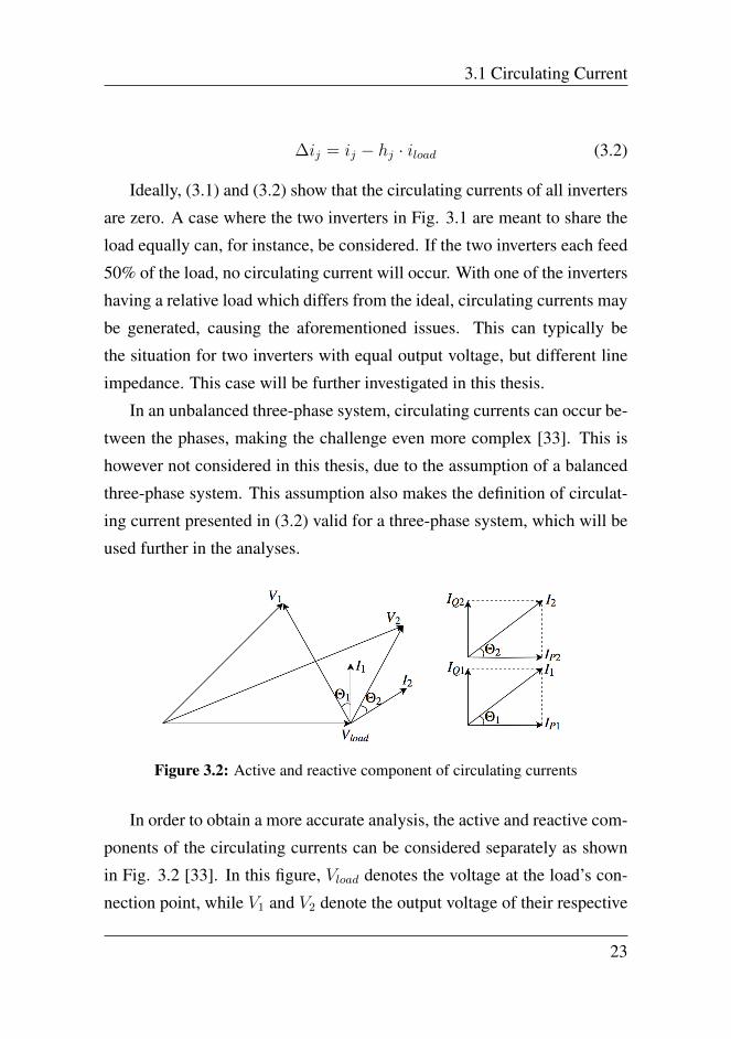
Figure 3.2: Active and reactive component of circulating currents
In order to obtain a more accurate analysis, the active and reactive com-
ponents of the circulating currents can be considered separately as shown
in Fig. 3.2 [33]. In this figure, Vload denotes the voltage at the load’s con-
nection point, while V1 and V2 denote the output voltage of their respective
23
Chapter 3. Power Flow Control
inverters. The output currents of the same inverters are given as I1 and
I2, where Θ denotes the angle between the voltage and the current. Each
of the currents can be divided into an active and reactive component, with
subscript P and Q, respectively. The difference between the two invert-
ers active output current will give the active circulating current, while the
difference between the reactive currents will give the reactive circulating
current.
This classification is done in [34], where the analysis shows which pa-
rameters effect the active and reactive power flow. Here, a two-inverter
system with equal phase voltages and similar line impedances is assumed.
The paper shows that a difference in output voltage may cause both active
and reactive circulating currents. The effect of these two components is de-
pendent on the grid’s R/X-ratio, in addition to the control methods used. In
order to design a control system which limits the generation of circulating
currents, a more thorough analysis of the active and reactive power flow is
given in Section 3.4.1.
In the following, this thesis will focus on minimizing steady state circu-
lating currents. Virtual impedance in addition to droop control can be used
for this purpose [34] [35]. Due to its good power sharing results and the
applicability for a decentralized control approach [36], this combination is
also the preferred method in this work. The next sections will give detailed
explanations of these methods and their control techniques.
3.2 Hierarchical Control Structure
In islanded microgrids, which mainly consist of paralleled DG units and
loads, the main control tasks include maintaining stable voltage and fre-
quency, in addition to power flow control. Stability challenges tend to be
more challenging in an islanded microgrid than in a grid-connected micro-
24

3.2 Hierarchical Control Structure
grid, due to no stiff, stabilizing grid [37]. Several approaches can be used
for controlling the microgrid, where a hierarchical control structure is cho-
sen in this work.
As presented in [38], a hierarchical control structure can be divided
into four different levels, numbered from zero to three. The control speed
decreases with increasing level, where the level zero has the fastest control
loop [6]. A representation of the different control levels is illustrated in
Fig. 3.3, which shows that the higher levels of control are dependent on the
lower.
Figure 3.3: Hierarchircal control structure
The inner control loops are at level zero, which include the local con-
trol for each device. This control level includes the inverter’s current and
voltage control which are necessary to keep the system stable. Level one,
the primary control, focuses on the microgrid as a whole, and makes sure
the interaction between paralleled inverters is sufficient. Droop control and
the use of virtual impedance operate on this level of control.
The secondary and tertiary control represent the two uppermost levels.
The secondary control secures that the electrical levels are within certain
limits. It can also make sure that the microgrid is synchronized with the
25

Chapter 3. Power Flow Control
main grid. Tertiary control is present in case of a grid-connected microgrid.
This level controls the exchange of energy between the main grid and the
microgrid.
The various control levels can be utilized differently. The mechanisms
can be based on a centralized control, a master slave control, or a decen-
tralized control [39]. In this thesis, a decentralized control is chosen on the
background of having an easily expandable system with plug-and-play ca-
pability. Decentralized control can be utilized through a controller with or
without communication, where this thesis is focused on a communication-
less controller in the primary control. This choice is motivated by the same
arguments as for choosing the decentralized approach. In addition to these
arguments, motivations for this approach are that a communication-less
controller will be more reliable in case of downtime and to avoid the costly
alternative of long distance communication lines [9, chapter 3].
In the following, this chapter will provide detailed explanations of the
control systems, which aim for sufficient power sharing in the islanded mi-
crogrid.
3.3 Inner control
The inner control is responsible for the voltage and current levels at the
output of the inverters. For each inverter, the current through the inverter-
side inductor and the voltage across the capacitor in the LCL-filter are con-
trolled. This is done through a cascaded control structure, by using the syn-
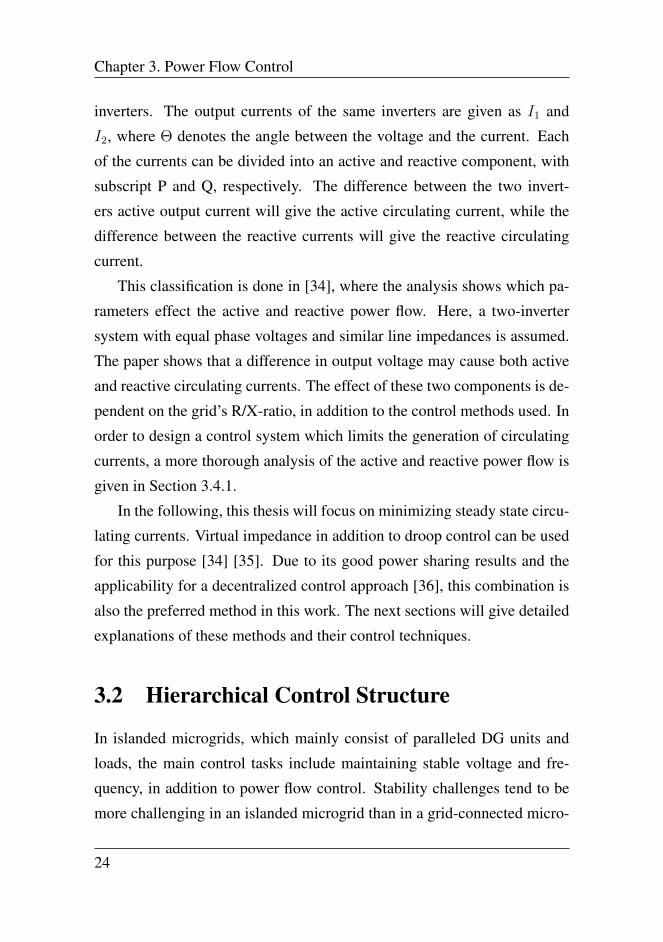
chronous reference frame [40]. The control structure is shown in Fig. 3.4.
The synchronous reference frame gives stationary quantities in a balanced
system. Since PI-controllers provide zero steady-state error with such quan-
tities, they are chosen for the controllers [41, chapter 9]. A description of
the synchronous reference frame is given in App. A.
26
3.3 Inner control
Figure 3.4: The cascaded control loop
Since an islanded mode of operation is considered, the voltage level
is completely controlled by the inverters in the microgrid. In this mode
of operation, the voltage control is the main objective of the inner control
loops. In the next sections, the structure of these control loops will be
presented.
3.3.1 Vector Control
The control system is based on the synchronous reference frame, where
a vector control principle is used to achieve accurate voltage and current
control. By having the d-axis aligned with the reference voltage vector [42,
chapter 5] and using a per-unit representation, the reference voltage vector’s
d-axis component is equal to the per-unit voltage level. Since the q-axis is
90 shifted from the reference voltage vector, its q-axis component is equal
to zero. The assumption of a balanced three-phase system makes the 0-
component always equal to zero. Therefore the 0-component is omitted in
this thesis.
27
Chapter 3. Power Flow Control
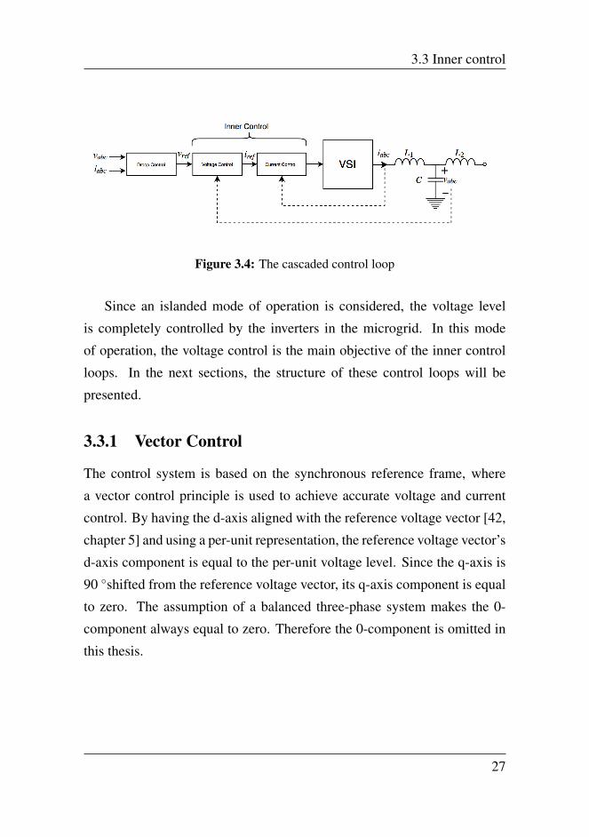
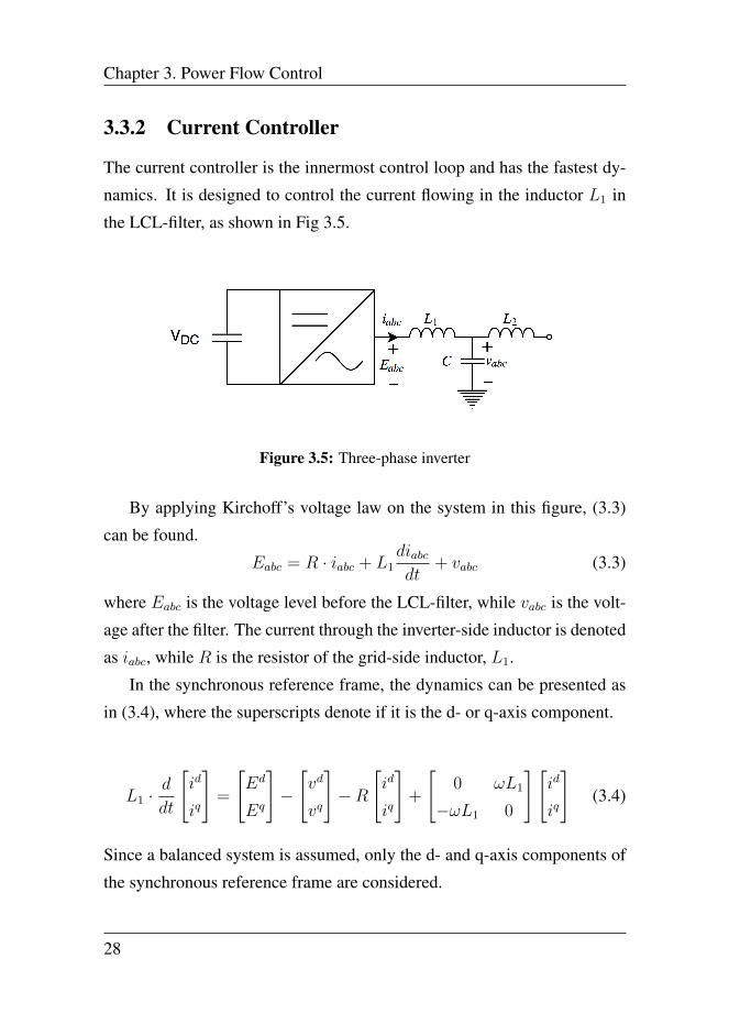
3.3.2 Current Controller
The current controller is the innermost control loop and has the fastest dy-
namics. It is designed to control the current flowing in the inductor L1 in
the LCL-filter, as shown in Fig 3.5.
Figure 3.5: Three-phase inverter
By applying Kirchoff’s voltage law on the system in this figure, (3.3)
can be found.
Eabc = R · iabc + L1diabcdt
+ vabc (3.3)
where Eabc is the voltage level before the LCL-filter, while vabc is the volt-
age after the filter. The current through the inverter-side inductor is denoted
as iabc, while R is the resistor of the grid-side inductor, L1.
In the synchronous reference frame, the dynamics can be presented as
in (3.4), where the superscripts denote if it is the d- or q-axis component.
L1 ·d
dt
[id
iq
]=
[Ed
Eq
]−
[vd
vq
]−R
[id
iq
]+
[0 ωL1
−ωL1 0
][id
iq
](3.4)
Since a balanced system is assumed, only the d- and q-axis components of
the synchronous reference frame are considered.
28
3.3 Inner control
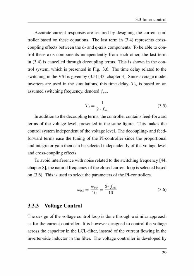
Accurate current responses are secured by designing the current con-
troller based on these equations. The last term in (3.4) represents cross-
coupling effects between the d- and q-axis components. To be able to con-
trol these axis components independently from each other, the last term
in (3.4) is cancelled through decoupling terms. This is shown in the con-
trol system, which is presented in Fig. 3.6. The time delay related to the
switching in the VSI is given by (3.5) [43, chapter 3]. Since average model
inverters are used in the simulations, this time delay, Td, is based on an
assumed switching frequency, denoted fsw.
Td =1
2 · fsw(3.5)
In addition to the decoupling terms, the controller contains feed-forward
terms of the voltage level, presented in the same figure. This makes the
control system independent of the voltage level. The decoupling- and feed-
forward terms ease the tuning of the PI-controller since the proportional
and integrator gain then can be selected independently of the voltage level
and cross-coupling effects.
To avoid interference with noise related to the switching frequency [44,
chapter 8], the natural frequency of the closed current loop is selected based
on (3.6). This is used to select the parameters of the PI-controllers.
ω0,i =wsw10
=2πfsw
10(3.6)
3.3.3 Voltage Control
The design of the voltage control loop is done through a similar approach
as for the current controller. It is however designed to control the voltage
across the capacitor in the LCL-filter, instead of the current flowing in the
inverter-side inductor in the filter. The voltage controller is developed by
29

Chapter 3. Power Flow Control
(a) d-axis
(b) q-axis
Figure 3.6: Block diagrams showing the current controller
30
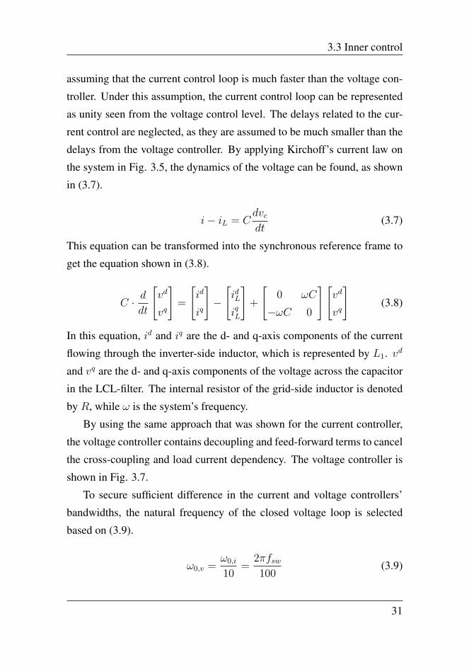
3.3 Inner control
assuming that the current control loop is much faster than the voltage con-
troller. Under this assumption, the current control loop can be represented
as unity seen from the voltage control level. The delays related to the cur-
rent control are neglected, as they are assumed to be much smaller than the
delays from the voltage controller. By applying Kirchoff’s current law on
the system in Fig. 3.5, the dynamics of the voltage can be found, as shown
in (3.7).
i− iL = Cdvcdt
(3.7)
This equation can be transformed into the synchronous reference frame to
get the equation shown in (3.8).
C · ddt
[vd
vq
]=
[id
iq
]−
[idL
iqL
]+
[0 ωC
−ωC 0
][vd
vq
](3.8)
In this equation, id and iq are the d- and q-axis components of the current
flowing through the inverter-side inductor, which is represented by L1. vd
and vq are the d- and q-axis components of the voltage across the capacitor
in the LCL-filter. The internal resistor of the grid-side inductor is denoted
by R, while ω is the system’s frequency.
By using the same approach that was shown for the current controller,
the voltage controller contains decoupling and feed-forward terms to cancel
the cross-coupling and load current dependency. The voltage controller is
shown in Fig. 3.7.
To secure sufficient difference in the current and voltage controllers’
bandwidths, the natural frequency of the closed voltage loop is selected
based on (3.9).
ω0,v =ω0,i
10=
2πfsw100
(3.9)
31

Chapter 3. Power Flow Control
(a) d-axis
(b) q-axis
Figure 3.7: Block diagrams showing the voltage controller
3.3.4 PI-Controllers
The implementation of current and voltage controllers is done through a
classical setup with a PI-controller in series with the electrical system. A
feedback of the relevant quantity is given, as shown in Fig. 3.8. In order to
obtain a fast and accurate response, the proportional- and integrator gain of
32

3.3 Inner control
Figure 3.8: General block diagram for the approach for the inner controllers
the PI-controller have to be selected carefully.
In the selection of these parameters, a pole placement method is uti-
lized. This entails an approximation of the physical process, expressing the
process by the dominant pole only. Consequently, the decoupling terms
explained for the voltage- and current controllers are assumed to ideally
compensate for the cross-coupling effects. Delays related to switching are
neglected in the current controller, while the inner current loop is repre-
sented as unity when designing the voltage controller. The electrical sys-
tems can then be presented as the transfer function shown in (3.10), where
the constants c1 and c2 are defined based on the specific system [45].
Gdominant =c1
s+ c2(3.10)
The tuning of the PI-controllers is decided based on the characteristic
polynomial in the denominator of the closed-loop transfer function, given
by (3.11) [41, chapter 4]. The closed loop transfer function is presented in
(3.12), where Kp and Ki are the parameters of the relevant PI-controller.
These parameters are equal for the controller on the d- and q-axis.
P (s) = s2 + 2ξω0s+ ω20 (3.11)
33

Chapter 3. Power Flow Control
Gcl =Ki · c1 +Kp · c1s
s2 + (c2 +Kp · c1)s+Ki · c1(3.12)
By combining (3.11) and (3.12), the parameters of the PI-controller can
be decided by (3.13) and (3.14).
Kp =2ξω0 − c2
c1(3.13)
Ki =ω20
c1(3.14)
The damping coefficient, ξ, is chosen to 0.7 both for the voltage and
current controller, in order to achieve well damped oscillations and rela-
tive low overshoot [41, chapter 4]. The natural frequency, ω0, can then be
decided for each controller to get the desired response.
The tuning of the PI-controllers used in the current- and voltage control
loops is shown in App. E, and bode plots showing the stability margins are
shown in App. F. The MATLAB-code for making these plots are given in
App. G.
3.4 Primary Control
The primary control level takes care of the interaction between inverters in
the islanded microgrid considered in this thesis. This is done through con-
trol of the voltage and frequency levels. With a distributed and communication-
less control approach, the primary control is based on measurements per-
formed locally at the inverters. The use of droop control methods is exam-
ined. This section presents the algorithms utilized, including in-depth ex-
planations about the use of virtual impedance for power sharing purposes.
34
3.4 Primary Control
3.4.1 Droop Control
Droop control algorithms seem promising in order to accommodate the
aforementioned objectives for the microgrid under investigation [36], and
are therefore chosen to be used in the primary control loop. Through the
study of different cases for the microgrid, two different methods are uti-
lized: The conventional and the opposite droop control. These will be pre-
sented in this section.
Without a need for communication between inverters, droop control
takes advantage of the relation between the voltage and the frequency in
the grid, and the power supplied by the inverters [46, chapter 9] [39]. The
frequency and voltage levels communicate if there is under- or overproduc-
tion in the microgrid, which is used to adjust the power supplied by the
inverters. This is done through a higher level of control, by adjusting the
set points for active and reactive power.
The droop control is located at the inverters, where the operation of each
unit will adapt to the entire system. Because of this, the control strategy is
well suited for expansions in the grid. Since the utilization of droop control
does not require high-speed communication, this may lead to significant
reductions in costs compared to a centralized controller [9, chapter 3], in
addition to high reliability.
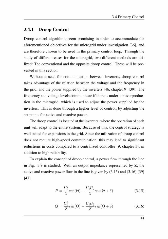
To explain the concept of droop control, a power flow through the line
in Fig. 3.9 is studied. With an output impedance represented by Z, the
active and reactive power flow in the line is given by (3.15) and (3.16) [39]
[47].
P =U21
Zcos(Θ)− U1U2
Zcos(Θ + δ) (3.15)
Q =U21
Zsin(Θ)− U1U2
Zsin(Θ + δ) (3.16)
35

Chapter 3. Power Flow Control
Figure 3.9: A representation of power flow through a distribution line
δ represents the power angle, while Θ is the angle of the output impedance,
Z. U1 and U2 are the voltage levels at the respective locations shown in Fig.
3.9. In a low-voltage microgrid, the output impedance is often dominated
by a resistive component.
All components located between the inverter’s output and the load are a
part of the inverter’s output impedance [48]. Even if the line has a resistive
behavior, these components, such as transformers and filters, will also con-
tribute to the output impedance. In the microgrid considered in this work,
LCL-filters are located at the output of the inverters, and the grid-side in-
ductor will contribute to the output impedance, making it more inductive
[36].
In the following, inverters with a dominating inductive output impedance
will be considered, leading to the conventional droop control method. In
addition, the opposite droop control method will be derived, which is based
on an output impedance dominated by a resistive component. Both methods
are derived based on (3.15) and (3.16).
36
3.4 Primary Control
Conventional Droop Control
Even if most low-voltage microgrids have line impedances dominated by a
resistive term, components such as transformers and LCL-filters can con-
tribute to a more inductive behavior. In the case of small line impedances,
the output impedance can become predominantly inductive.
With inductive output impedances, the conventional droop control method
can be used to control the power sharing. In the derivation of this method,
(3.15) and (3.16) form the basis, in addition to two important assumptions:
The output impedance is purely inductive. This makes the impedance in
(3.15) and (3.16), Z, equal to a pure reactance, X . The impedance angle,
Θ, will then be equal to 90.
The power angle, δ, is assumed to be small. This assumption is done on
the background of a relatively small phase difference between the voltage
at the output of the inverter and at the loads’ connection point. By this,
sin(δ) ' δ and cos(δ) ' 1 can be used in the derivations.
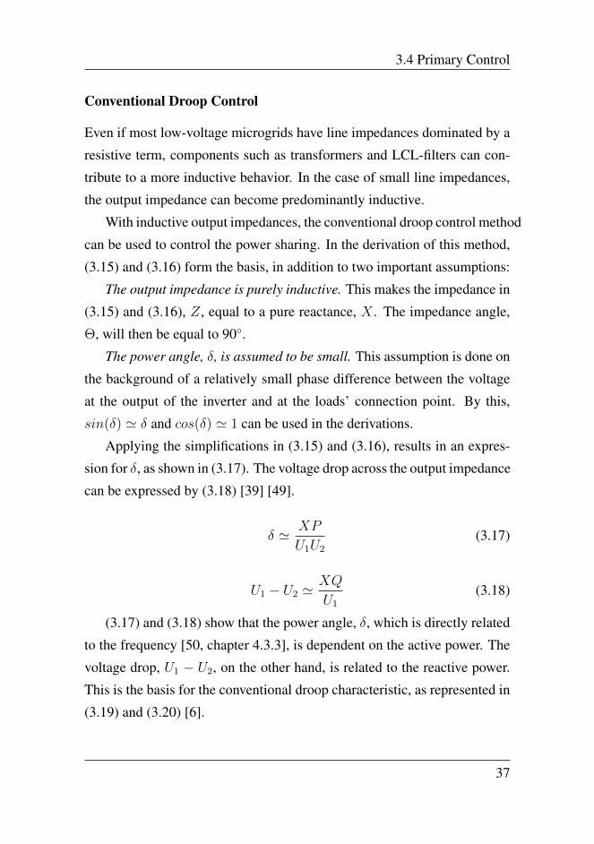
Applying the simplifications in (3.15) and (3.16), results in an expres-
sion for δ, as shown in (3.17). The voltage drop across the output impedance
can be expressed by (3.18) [39] [49].
δ ' XP
U1U2
(3.17)
U1 − U2 'XQ
U1
(3.18)
(3.17) and (3.18) show that the power angle, δ, which is directly related
to the frequency [50, chapter 4.3.3], is dependent on the active power. The
voltage drop, U1 − U2, on the other hand, is related to the reactive power.
This is the basis for the conventional droop characteristic, as represented in
(3.19) and (3.20) [6].
37
Chapter 3. Power Flow Control
ω − ωref = mP (Pref − P ) (3.19)
E − Eref = nQ(Qref −Q) (3.20)
This characteristic is based on a rated voltage and frequency, denoted
Eref and ωref . The active and reactive droop coefficients are given as mP
and nQ. They decide the relation between frequency and active power, and
voltage and reactive power, respectively. E, ω, P and Q are the measured
values of voltage, frequency, active power and reactive power. Pref and
Qref are the set points for active and reactive power [39]. These are deter-
mined by a higher level of control, which normally is dependent on com-
munication in order to adapt to the load of the system [51]. These upper
levels of control are beyond scope of this thesis. The conventional droop
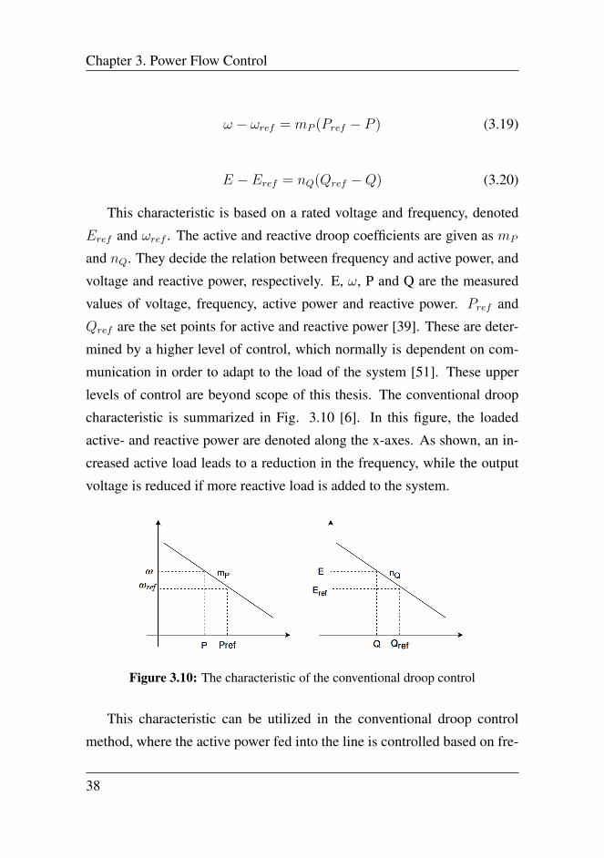
characteristic is summarized in Fig. 3.10 [6]. In this figure, the loaded
active- and reactive power are denoted along the x-axes. As shown, an in-
creased active load leads to a reduction in the frequency, while the output
voltage is reduced if more reactive load is added to the system.
Figure 3.10: The characteristic of the conventional droop control
This characteristic can be utilized in the conventional droop control
method, where the active power fed into the line is controlled based on fre-
38
3.4 Primary Control
quency deviations, while deviations in voltage control the reactive power
supply [52] [39]. The deviations are determined by the droop coefficients,
which are given based on (3.21) and (3.22) [36].
mP =∆ωmaxPchange
(3.21)
nQ =∆EmaxQchange
(3.22)
∆ωmax is the maximum allowed frequency deviation due to a load
change in active power, Pchange. The maximum allowed voltage change,
∆Emax, is in a similar way related to a load change in reactive power,
Qchange. Often, ∆ωmax and ∆Emax are decided based on the maximum
deviations allowed in the grid [36]. The droop coefficients also affect the
power sharing among inverters, where larger droop coefficients lead to bet-
ter power sharing. However, the coefficients have upper limits, where in-
creasing them would lead to instability in the system [53]. Within the stabil-
ity limits, the choice of droop coefficients is a trade-off between the power
sharing performance and the deviations in voltage and frequency. The re-
lation between the droop coefficients of different inverters will be equal to
the relation between the power supplied from the same inverters in an ideal
microgrid. In order to make two DG units share the power equally, the
droop coefficients should, therefore, be designed equally in size.
With close to purely inductive output impedances, the conventional
droop control method is an effective way to adjust frequency and voltage
relative to the supplied power. While the active power is shared equally
among inverters, this method has certain challenges related to reactive power
sharing. A difference in output voltage or output impedances, which can
occur with distribution lines of different lengths, often causes unequal re-
active power supply from the inverters [36] [54]. As a result, reactive cir-
39
Chapter 3. Power Flow Control
culating currents are generated. This is one of the challenges to be further
investigated in this thesis, including a study of how virtual impedance can
be utilized to minimize these circulating currents.
A real distribution line will always contain a combination of resistive
and inductive components. However, purely inductive distribution lines can
cause an unstable response, as discussed in [9, chapter 3]. This enhances
the importance of choosing realistic values for the output impedances, in-
cluding a combination of resistance and reactance. It also has to be taken
into consideration when deciding the virtual impedance values, which will
be further discussed later in this thesis.
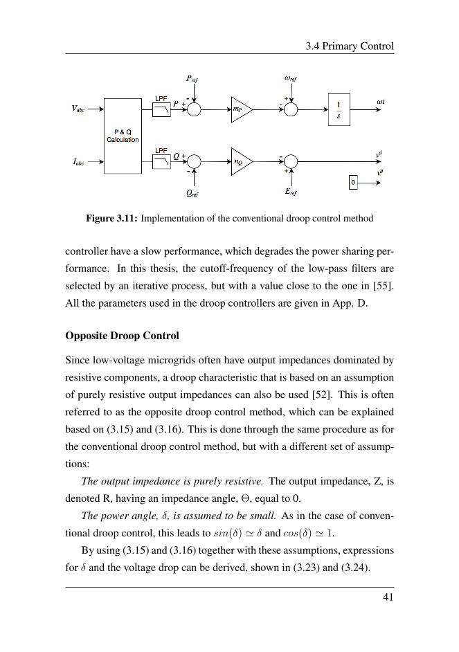
In the case studies presented in Chapter 4, the implementation of a con-
ventional droop controller is as shown in Fig. 3.11. The basis of the con-
troller is the conventional droop characteristic, given by (3.19) and (3.20).
The droop coefficients, mP and nQ, are selected based on (3.21) and (3.22).
In case of a load change equal to half a residential load, the frequency and
voltage deviations are selected to be 0.1 Hz and 2.3 V, respectively.
Figure 3.11 shows that only the d-axis component of the voltage, vd,
is related to the droop characteristic, while the q-axis component, vq, is
forced to be zero. The output frequency obtained from the droop controller
is integrated, which gives a constantly changing angle, ωt. This angle is
used in the transformation between the abc- and the synchronous reference
frame. By utilizing this approach, the voltage vectors at the output of the
inverters are aligned with the d-axis in the synchronous reference frame.
For a review of the synchronous reference frame, see App. A.
As shown in Fig. 3.11, the measured active and reactive power are
filtered through low-pass filters. This makes the droop controller less af-
fected by high frequency components in the system, and contributes to a
sufficient difference in bandwidth between the inner control loops and the
droop controller [55]. However, a low cutoff-frequency will make the droop
40
3.4 Primary Control
Figure 3.11: Implementation of the conventional droop control method
controller have a slow performance, which degrades the power sharing per-
formance. In this thesis, the cutoff-frequency of the low-pass filters are
selected by an iterative process, but with a value close to the one in [55].
All the parameters used in the droop controllers are given in App. D.
Opposite Droop Control
Since low-voltage microgrids often have output impedances dominated by
resistive components, a droop characteristic that is based on an assumption
of purely resistive output impedances can also be used [52]. This is often
referred to as the opposite droop control method, which can be explained
based on (3.15) and (3.16). This is done through the same procedure as for
the conventional droop control method, but with a different set of assump-
tions:
The output impedance is purely resistive. The output impedance, Z, is
denoted R, having an impedance angle, Θ, equal to 0.
The power angle, δ, is assumed to be small. As in the case of conven-
tional droop control, this leads to sin(δ) ' δ and cos(δ) ' 1.
By using (3.15) and (3.16) together with these assumptions, expressions
for δ and the voltage drop can be derived, shown in (3.23) and (3.24).
41

Chapter 3. Power Flow Control
δ ' − RQ
U1U2
(3.23)
U1 − U2 'RP
U1
(3.24)
Compared to the conventional droop characteristic, (3.23) and (3.24)
show opposite relations: The power angle, δ, and hence the frequency, are
dependent on the reactive power, while the voltage drop depends on the
active power [39] [56]. This is the basis of the opposite droop control, with
characteristic given by (3.25) and (3.26) [52].
ω − ωref = mQ(Q−Qref ) (3.25)
E − Eref = nP (Pref − P ) (3.26)
The droop coefficients are denoted nP and mQ, and are shown graphically
in Fig. 3.12.
Figure 3.12: The characteristic of the opposite droop control
As for the conventional droop control, the droop coefficients are chosen
based on active and reactive power change, and maximum deviations in
voltage and frequency related to these changes. The design is then given
42

3.4 Primary Control
as shown in (3.27) and (3.28). The coefficients can, in the same way as for
the conventional droop control, be used to control the power sharing among
inverters.
mQ =∆ωmaxQchange
(3.27)
nP =∆EmaxPchange
(3.28)
The opposite droop characteristic has a direct relation between the volt-
age drop across the output impedance and the active power flow. Because
of this, two inverters with mismatching output impedance will induce active
circulating currents. This is analogous to the conventional droop control’s
power sharing, but the circulating currents are related to the active power
flow instead of the reactive. The opposite droop control has advantages
compared to the conventional droop control when it comes to direct volt-
age control [52] and harmonic power sharing [56]. The overall system is
more damped, and phase errors will hardly affect the active power shar-
ing [56]. Because of the above-mentioned advantages, the opposite droop
control algorithm may be preferred over the conventional droop control in
some cases. However, the conventional droop control is more commonly
used, for instance because of better active power sharing [9, chapter 3].
In the modelling that will be presented in Chapter 4, the opposite droop
control is implemented as shown in Fig. 3.13. The control is similar to
the conventional droop control, with the voltage vector aligned with the
synchronous reference frame, and based on the relations given in (3.25)
and (3.26). As for the conventional droop control, low-pass filters are used
to filter the measured output power. Both the low-pass filters and the criteria
used to design the droop coefficients are the same, and is given in App. D.
Mismatching output voltages and physical output impedances are ele-
43

Chapter 3. Power Flow Control
Figure 3.13: Implementation of the opposite droop control method
ments that affect the power sharing when using droop control algorithms,
where another is the angle of the physical output impedance. Challenges
related to this are presented in the following section.
3.4.2 Mixed Output Impedance
When using local measurements for voltage and frequency, it is convenient
to utilize the mentioned droop control algorithms for a decentralized control
approach. When it comes to power sharing, the challenges related to dif-
ferences in output impedances have already been mentioned. The charac-
teristics of the conventional and opposite droops are based on assumptions
of either a purely inductive or purely resistive output impedance. In a real
microgrid, the output impedance exists of both resistance and reactance,
as described in Section 2.4. This results in a coupling between active and
reactive power, making both of them depending on voltage and frequency
levels [57]. More complicated power sharing challenges are then present,
with many proposed solutions reviewed in [57].
Since the conventional droop control is based on the assumption of
purely inductive output impedances, several issues arise when the control
method is applied in systems with resistive or mixed output impedances.
44
3.4 Primary Control
The conventional droop control used in a system with predominantly re-
sistive output impedances can provide a stable and well functional perfor-
mance, as discussed in [54]. However, the stability margins are smaller,
and the challenges related to reactive power sharing often increase when
having predominantly resistive output impedances while using the conven-
tional droop control [54]. If the control parameters are not selected care-
fully, stability issues often arise, especially when having local loads and
large output impedances [58] [59]. The active power has a minor effect
on the stability challenges, while the reactive droop coefficient nQ and the
output resistance is of great importance. According to [58], the use of con-
ventional droop control in a predominantly resistive microgrid provides bad
transient behavior for the power control in grid-connected mode. In island
mode, the challenges are even more complicated, causing worse reactive
power sharing and increased stability issues.
Also when applying the opposite droop control to a predominantly in-
ductive output impedance, issues related to stability appear. The opposite
droop control is rarely used in microgrids with predominantly inductive
output impedances, because of these stability challenges and the impor-
tance of accurate active power dispatch. The conventional droop control’s
similar behavior and compatibility with synchronous generators are often
preferable [52], in addition to the accurate active power sharing. By select-
ing the droop coefficients carefully, the conventional droop control can pro-
vide virtual inertia to the system [60]. However, there are cases where the
opposite droop control’s direct voltage control is preferable, in addition to
the more stable operation with predominantly resistive output impedances
[52] [54].
Even if the droop control algorithms provide unstable responses with
certain output impedances, the use of virtual impedances is an effective
method to modify the output impedance of the inverters. It can effec-
45
Chapter 3. Power Flow Control
tively achieve stable, well performing responses, almost regardless of the
actual output impedance of the inverters [61]. In the following sections,
power sharing issues will be further investigated through the use of vir-
tual impedances as a part of the inverters’ control system. The output
impedance of an inverter will be denoted by physical output impedance,
in order to avoid confusion when the concept of virtual impedance is intro-
duced. The combination of physical output impedance and virtual impedance
is denoted by equivalent output impedance.
3.4.3 Virtual Impedance
The previous sections have explained concepts and challenges related to
power sharing in islanded microgrids. This section will elaborate on tech-
niques used to improve the power sharing. Virtual impedance is a control
mechanism which is frequently used for this purpose, often in combination
with droop control [36] [62]. This is also the focus of this thesis. An intro-
duction to virtual impedances, including different areas of utilization will
be given in this section. Design considerations, both for existing methods
and proposed virtual impedance methods will be presented. The implemen-
tation of the virtual impedances used in the simulation models is explained.
In addition to power sharing, virtual impedances are used in converter
control for applications such as harmonic voltage compensation and in-
creased stability [63]. The concept is divided into two categories in [63]:
Inner- and outer virtual impedance. Inner virtual impedance-loops are used
for harmonic compensations and current limiting purposes, and the sig-
nal from the loop is applied at the PWM. Harmonic voltage compensation,
control of power flow, mitigation of unbalanced voltage and sharing be-
tween nonlinear loads in a power system are done by the use of outer virtual
impedance, which modifies the reference signal of the controller.
The two categories of virtual impedances are both used to shape the
46

3.4 Primary Control
equivalent output impedance of the converter. Because of its many applica-
tions, the value of this impedance has to be decided based on its purpose. In
[64], the values of the virtual impedances are studied in order to optimize
the microgrid’s performance. The virtual impedances can help to keep the
voltage within certain limits, have sufficient reactive power sharing, provide
system damping and decouple the active and reactive power. In general, a
virtual impedance imitates the behaviour of an actual impedance, without
experiencing losses. The non-physical concept of negative impedance can
also be added to the inverters thorugh the use of virtual impedance [63].
Since this work is focused on the challenges related to power sharing
of fundamental components, the microgrid system presented in Chapter 2
will be used for the investigation of the use of virtual impedance in micro-
grid. The utilization of outer virtual impedance loops is studied in order to
improve power sharing between linear loads. First, an elaboration on outer
virtual impedance techniques will be performed. In the following, outer
virtual impedance is simply denoted virtual impedance.
Figure 3.14: Block diagram showing an outer virtual impedance loop
A diagram showing the general design for virtual impedance loops is
shown in Fig. 3.14 [62]. The voltage reference is modified by the output
current, Ioutput, and the virtual impedance, denoted by Zv. As shown in the
figure, the voltage reference from the droop control, V ∗, is subtracted a volt-
age drop caused by the virtual impedance, ∆Vv, which gives the reference
47

Chapter 3. Power Flow Control
to the inner control loops, Vref . This approach can both change the mag-
nitude and the impedance angle of the equivalent output impedance. The
selection of the virtual impedances have to be done carefully, both when
it comes to the relation between the resistive and reactive components, but
also regarding the impedances’ total size.
A distinct disadvantage of applying virtual impedances is their tendency
of reducing the voltage reference, as is evident from (3.29). This has to
be taken into consideration when the value of the impedance is selected.
By applying a combination of positive and negative virtual impedances,
this thesis will suggest virtual impedance designs that limit the negative
effects on the voltage. A thorough review of advantages and disadvantages
regarding virtual impedance in combination with droop control is given in
[36].
Vref = V ∗ −∆vv = V ∗ − Zv · Ioutput (3.29)
In (3.29), V ∗ denotes the voltage reference from the droop controller,
while ∆vv is the voltage drop due to the virtual impedance. Ioutput is the
output current and Zv the virtual impedance. Vref is the voltage reference
applied to the inner control.
Existing Designs
As mentioned above, virtual impedances are commonly used in combina-
tion with droop control algorithms in order to improve active and reactive
power sharing. The virtual impedances can be used to compensate for pos-
sible differences in physical output impedance among inverters. According
to literature, this method is effective both in terms of active and reactive
power sharing [65], because the two inverters get equal equivalent output
impedance. The virtual impedance is then selected to make the equiva-
48
3.4 Primary Control
lent output impedance, including the physical output impedance and virtual
impedance, be equal for all inverters in the system. The basic method can
be explained by (3.30), and is referred to as output impedance matching
[65]. Zo,i denotes the output impedance of inverter i, which is the sum of
all impedances between the inverters’ output and the load, as seen from the
inverter. The virtual impedance applied to inverter i is referred to as Zv,i.
Zo,1 + Zv,1 = Zo,2 + Zv,2 (3.30)
Virtual impedance can also be used with the primary goal of chang-
ing the impedance angle of the equivalent output impedance. When utiliz-
ing the conventional droop control, positive inductive- or negative resistive
virtual impedances can be added to low-voltage grids in order to provide
inductive equivalent output impedance for the inverters [47] [66] [67]. In
addition, this may contribute to increasing the stability margins [54]. The
method takes advantage of the conventional droop control’s accurate ac-
tive power sharing. This method is often preferred rather than the opposite
droop when the physical output impedances are dominated by predomi-
nantly resistive line impedances [9, chapter 3].
A similar method can be utilized for the opposite droop control method,
but instead of a virtual inductor, the virtual impedance applied has a rela-
tively large resistive value [68] [56]. When virtual impedances are used
to make the equivalent output impedances have a more inductive or resis-
tive behavior, the size of the virtual impedances is normally selected to
dominate the physical output impedances [56] [9, chapter 3] [27]. This
ensures proper decoupling of the active and reactive power. In case of un-
equal physical output impedances of the inverters, the relative difference
between the equivalent output impedance is reduced, which has a positive
effect on the power sharing [56]. In addition to improving the power shar-
ing, the resistive virtual impedances contribute to an increased damping of
49
Chapter 3. Power Flow Control
the system [68].
Proposed Designs
With existing virtual impedance designs, power sharing is significantly im-
proved. However, the voltage drops related to these designs can be rela-
tively large [69]. This section will, therefore, propose virtual impedance
designs that are able to reduce the voltage drops.
The first proposed solution suggests a new virtual impedance design in
order to utilize output impedance matching, where one virtual impedance
is divided into two. In the approach taken in [9, chapter 3], a virtual
impedance is added to the inverter with the lower physical output impedance,
in order to make the equivalent output impedance of the two inverters equal.
If virtual impedances are added to both inverters, the voltage drop over
the virtual impedances can be heavily reduced. The proposed solution
for matching the output impedances includes a negative virtual impedance
at the inverter with the higher physical output impedance and a positive
virtual impedance added to the inverter with the lower physical output
impedance. Each virtual impedance is consequently half the value of the
virtual impedance that would be applied if using the existing design ap-
proach, with one virtual impedance only. Thus, the voltage drop due to the
use of virtual impedances will be significantly reduced by this method.
If virtual impedances are used to obtain predominantly inductive- or
resistive equivalent output impedance, the virtual impedances are often se-
lected to be relatively large. Because of their size, the virtual impedances
lead to a significant voltage drop. In order to reduce this voltage drop, a
solution including a complex virtual impedance are suggested.
When this second proposed solution is applied with the conventional
droop control, the virtual impedances include positive virtual inductors and
negative virtual resistors. The decoupling of active and reactive power
50
3.4 Primary Control
is by this technique even stronger than by using only inductive virtual
impedances. In addition, the voltage drops across the virtual impedances
are significantly reduced. The virtual resistor has to be selected smaller in
magnitude than the resistive part of the physical output impedance, to avoid
the equivalent output impedance to be purely inductive, which can lead to
an unstable behavior [9, chapter 3].
A similar approach can be taken when using the opposite droop con-
trol, where the virtual impedances will consist of a positive resistor and
negative inductor. The negative inductor is suggested equal in magnitude
as the largest physical output inductor, since the inductors do not contribute
to any stabilizing effect. The resistance is selected to be dominating com-
pared to the larger physical output impedance in the system, as for the more
conventionally used virtual impedance method.
In the following, the implementation of the virtual impedances used in
the modelling will be presented.
Implementation
With improved power sharing and limiting circulating currents as the main
objectives, this section will elaborate on how the virtual impedance loops
used in this work are implemented. The implementation of the virtual
impedance loops is done in the synchronous reference frame by using per
unit values. This makes the different levels of control compatible with
each other since the inner control loops are implemented in this way, as
explained in Section 3.3.
The applied virtual impedances are designed as resistive-inductive vir-
tual impedances, where the virtual voltage drop is represented in (3.31).
∆vvirtual,abc = R · iabc + Ldiabcdt
(3.31)
51

Chapter 3. Power Flow Control
In the implementation of virtual impedances, (3.31) is transformed to
the synchronous reference frame by using the park transform. This results
in (3.32), which leads to (3.33). Since the system is assumed to be balanced,
the 0-component is omitted in the virtual impedance implementation.
∆vvirtual,dq0 = Ridq0 + Ldidq0dt
+ jωLidq0 (3.32)
[∆vvirtual,d
∆vvirtual,q
]= R
[id
iq
]+ L · s
[id
iq
]+
[0 −ωLωL 0
][id
iq
](3.33)
In order to achieve a voltage level less affected by high-frequency os-
cillations, low pass-filters are used in the implementation. This is essential
when using these virtual impedance loops, due to the derivative term [63] in
(3.33). The filters contribute keeping the voltage drops caused by the virtual
impedance within reasonable limits, since the derivative terms and high-
frequency current components can cause large voltage deviations. Figure
3.15 shows the implementation of virtual impedance used in this work, in-
cluding the low-pass filters. A disadvantage of using the low-pass filters
is that they cause a phase shift that may change the behavior of the virtual
impedance [63]. The low-pass filters also cause a slightly slower dynamic
response, as they add an additional time delay to the system. The low-pass
filters used in the virtual impedance implementation is chosen with a cut-
off frequency which equals the frequency of third harmonic oscillations in
the system. The exact value is given in App. D.
In the next chapter, simulations verifying the effects of using virtual
impedance will be carried out. The proposed virtual impedance methods
will be compared to the existing virtual impedance methods covered by
the literature review. The power sharing and the output voltage level when
52

3.4 Primary Control
utilizing the different methods will be the primary focus in the analysis.
Figure 3.15: Schematic of the implementation of virtual impedance
53

Chapter 3. Power Flow Control
54

4 | Cases Studies
This chapter contains simulations for three different cases, in order to show
how virtual impedances can be used to improve power sharing and mitigate
circulating currents. Simulations are done for two different microgrid sys-
tems, both of which can be presented by the general system presented in
Chapter 2. Figures showing the models in Simulink is shown App. I and
responses of the different controllers utilized are demonstrated in App. H.
Case 1 presents a microgrid with predominantly resistive physical out-
put impedances, and the results from this case are presented in Section
4.2. This section is divided into two subsections, and includes simula-
tions where both conventional and opposite droop control is utilized in the
primary control loop. In case 2, the system has predominantly inductive
physical output impedances. The analysis performed is similar as in case
1, with two different subcases for utilizing two different primary control
loops. This is presented in Section 4.3. Case 3 is a reproduction of case 2,
but in the selection of virtual impedances, the physical output impedance
of the inverters is estimated to be 25 % lower than the actual values. This
is presented in Section 4.4.
In general, the simulations for each subcase can be divided into three:
1. The conventional- or opposite droop control method is utilized in the
primary control loop, without any use of virtual impedance.
55
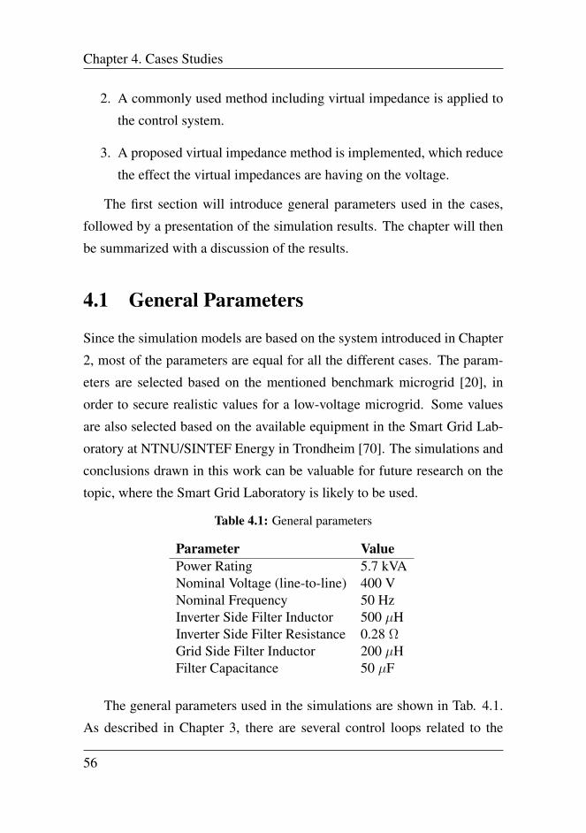
Chapter 4. Cases Studies
2. A commonly used method including virtual impedance is applied to
the control system.
3. A proposed virtual impedance method is implemented, which reduce
the effect the virtual impedances are having on the voltage.
The first section will introduce general parameters used in the cases,
followed by a presentation of the simulation results. The chapter will then
be summarized with a discussion of the results.
4.1 General Parameters
Since the simulation models are based on the system introduced in Chapter
2, most of the parameters are equal for all the different cases. The param-
eters are selected based on the mentioned benchmark microgrid [20], in
order to secure realistic values for a low-voltage microgrid. Some values
are also selected based on the available equipment in the Smart Grid Lab-
oratory at NTNU/SINTEF Energy in Trondheim [70]. The simulations and
conclusions drawn in this work can be valuable for future research on the
topic, where the Smart Grid Laboratory is likely to be used.
Table 4.1: General parameters
Parameter ValuePower Rating 5.7 kVANominal Voltage (line-to-line) 400 VNominal Frequency 50 HzInverter Side Filter Inductor 500 µHInverter Side Filter Resistance 0.28 ΩGrid Side Filter Inductor 200 µHFilter Capacitance 50 µF
The general parameters used in the simulations are shown in Tab. 4.1.
As described in Chapter 3, there are several control loops related to the
56
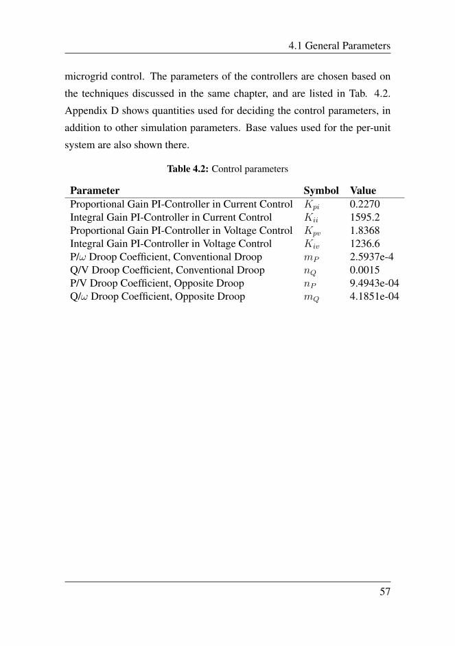
4.1 General Parameters
microgrid control. The parameters of the controllers are chosen based on
the techniques discussed in the same chapter, and are listed in Tab. 4.2.
Appendix D shows quantities used for deciding the control parameters, in
addition to other simulation parameters. Base values used for the per-unit
system are also shown there.
Table 4.2: Control parameters
Parameter Symbol ValueProportional Gain PI-Controller in Current Control Kpi 0.2270Integral Gain PI-Controller in Current Control Kii 1595.2Proportional Gain PI-Controller in Voltage Control Kpv 1.8368Integral Gain PI-Controller in Voltage Control Kiv 1236.6P/ω Droop Coefficient, Conventional Droop mP 2.5937e-4Q/V Droop Coefficient, Conventional Droop nQ 0.0015P/V Droop Coefficient, Opposite Droop nP 9.4943e-04Q/ω Droop Coefficient, Opposite Droop mQ 4.1851e-04
57
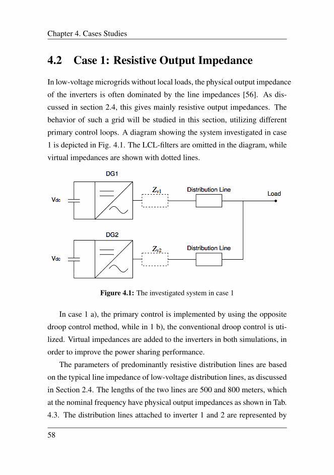
Chapter 4. Cases Studies
4.2 Case 1: Resistive Output Impedance
In low-voltage microgrids without local loads, the physical output impedance
of the inverters is often dominated by the line impedances [56]. As dis-
cussed in section 2.4, this gives mainly resistive output impedances. The
behavior of such a grid will be studied in this section, utilizing different
primary control loops. A diagram showing the system investigated in case
1 is depicted in Fig. 4.1. The LCL-filters are omitted in the diagram, while
virtual impedances are shown with dotted lines.
Figure 4.1: The investigated system in case 1
In case 1 a), the primary control is implemented by using the opposite
droop control method, while in 1 b), the conventional droop control is uti-
lized. Virtual impedances are added to the inverters in both simulations, in
order to improve the power sharing performance.
The parameters of predominantly resistive distribution lines are based
on the typical line impedance of low-voltage distribution lines, as discussed
in Section 2.4. The lengths of the two lines are 500 and 800 meters, which
at the nominal frequency have physical output impedances as shown in Tab.
4.3. The distribution lines attached to inverter 1 and 2 are represented by
58
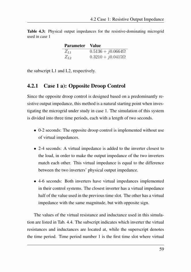
4.2 Case 1: Resistive Output Impedance
Table 4.3: Physical output impedances for the resistive-dominating microgridused in case 1
Parameter ValueZL1 0.5136 + j0.0664ΩZL2 0.3210 + j0.0415Ω
the subscript L1 and L2, respectively.
4.2.1 Case 1 a): Opposite Droop Control
Since the opposite droop control is designed based on a predominantly re-
sistive output impedance, this method is a natural starting point when inves-
tigating the microgrid under study in case 1. The simulation of this system
is divided into three time periods, each with a length of two seconds.
• 0-2 seconds: The opposite droop control is implemented without use
of virtual impedances.
• 2-4 seconds: A virtual impedance is added to the inverter closest to
the load, in order to make the output impedance of the two inverters
match each other. This virtual impedance is equal to the difference
between the two inverters’ physical output impedance.
• 4-6 seconds: Both inverters have virtual impedances implemented
in their control systems. The closest inverter has a virtual impedance
half of the value used in the previous time slot. The other has a virtual
impedance with the same magnitude, but with opposite sign.
The values of the virtual resistance and inductance used in this simula-
tion are listed in Tab. 4.4. The subscript indicates which inverter the virtual
resistances and inductances are located at, while the superscript denotes
the time period. Time period number 1 is the first time slot where virtual
59
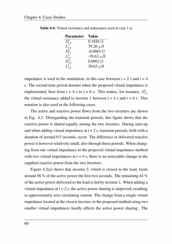
Chapter 4. Cases Studies
Table 4.4: Virtual resistance and inductance used in case 1 a)
Parameter ValueR1v2 0.1926 Ω
L1v2 79.26 µH
R2v1 -0.0963 Ω
L2v1 -39.63 µH
R2v2 0.0963 Ω
L2v2 39.63 µH
impedance is used in the simulation, in this case between t = 2 s and t = 4
s. The second time period denotes when the proposed virtual impedance is
implemented, here from t = 4 s to t = 6 s. This makes, for instance, R2v1
the virtual resistance added to inverter 1 between t = 4 s and t = 6 s. This
notation is also used in the following cases.
The active and reactive power flows from the two inverters are shown
in Fig. 4.2. Disregarding the transient periods, this figure shows that the
reactive power is shared equally among the two inverters. During start-up
and when adding virtual impedance at t = 2 s, transient periods, both with a
duration of around 0.5 seconds, occur. The difference in delivered reactive
power is however relatively small, also through these periods. When chang-
ing from one virtual impedance to the proposed virtual impedance method
with two virtual impedances at t = 4 s, there is no noticeable change in the
supplied reactive power from the two inverters.
Figure 4.2(a) shows that inverter 2, which is closest to the load, feeds
around 56 % of the active power the first two seconds. The remaining 44 %
of the active power delivered to the load is fed by inverter 1. When adding a
virtual impedance at t = 2 s, the active power sharing is improved, resulting
in approximately zero circulating current. The change from a single virtual
impedance located at the closest inverter, to the proposed method using two
smaller virtual impedances hardly affects the active power sharing. The
60
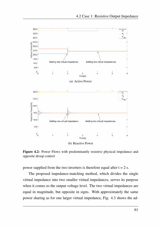
4.2 Case 1: Resistive Output Impedance
(a) Active Power
(b) Reactive Power
Figure 4.2: Power Flows with predominantly resistive physical impedance andopposite droop control
power supplied from the two inverters is therefore equal after t = 2 s.
The proposed impedance-matching method, which divides the single
virtual impedance into two smaller virtual impedances, serves its purpose
when it comes to the output voltage level. The two virtual impedances are
equal in magnitude, but opposite in signs. With approximately the same
power sharing as for one larger virtual impedance, Fig. 4.3 shows the ad-
61
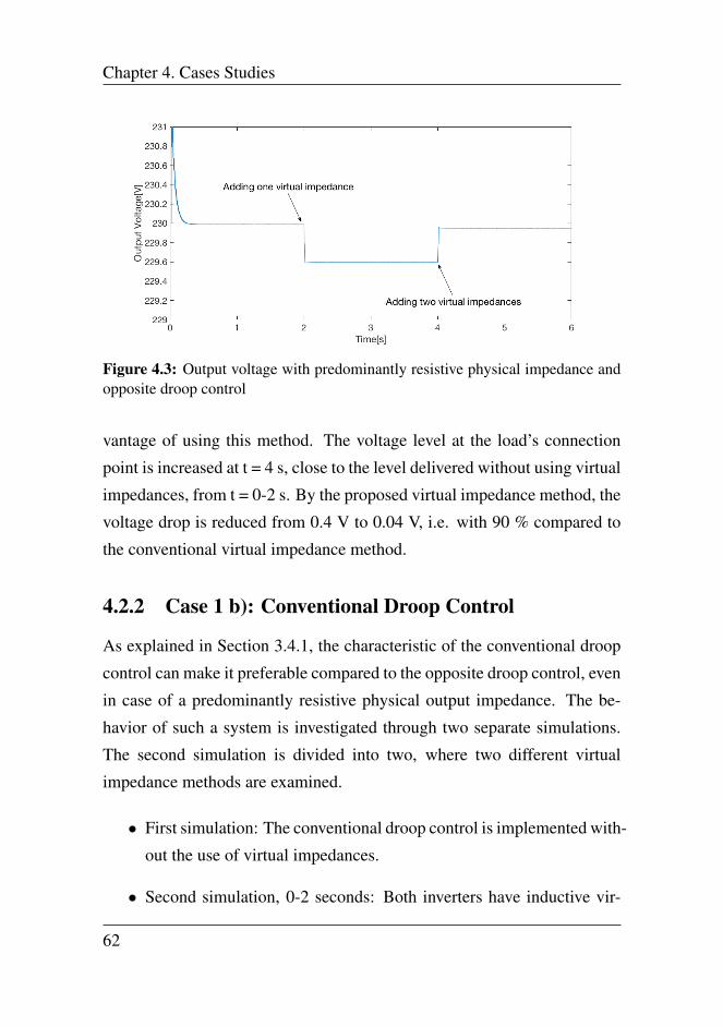
Chapter 4. Cases Studies
Figure 4.3: Output voltage with predominantly resistive physical impedance andopposite droop control
vantage of using this method. The voltage level at the load’s connection
point is increased at t = 4 s, close to the level delivered without using virtual
impedances, from t = 0-2 s. By the proposed virtual impedance method, the
voltage drop is reduced from 0.4 V to 0.04 V, i.e. with 90 % compared to
the conventional virtual impedance method.
4.2.2 Case 1 b): Conventional Droop Control
As explained in Section 3.4.1, the characteristic of the conventional droop
control can make it preferable compared to the opposite droop control, even
in case of a predominantly resistive physical output impedance. The be-
havior of such a system is investigated through two separate simulations.
The second simulation is divided into two, where two different virtual
impedance methods are examined.
• First simulation: The conventional droop control is implemented with-
out the use of virtual impedances.
• Second simulation, 0-2 seconds: Both inverters have inductive vir-
62
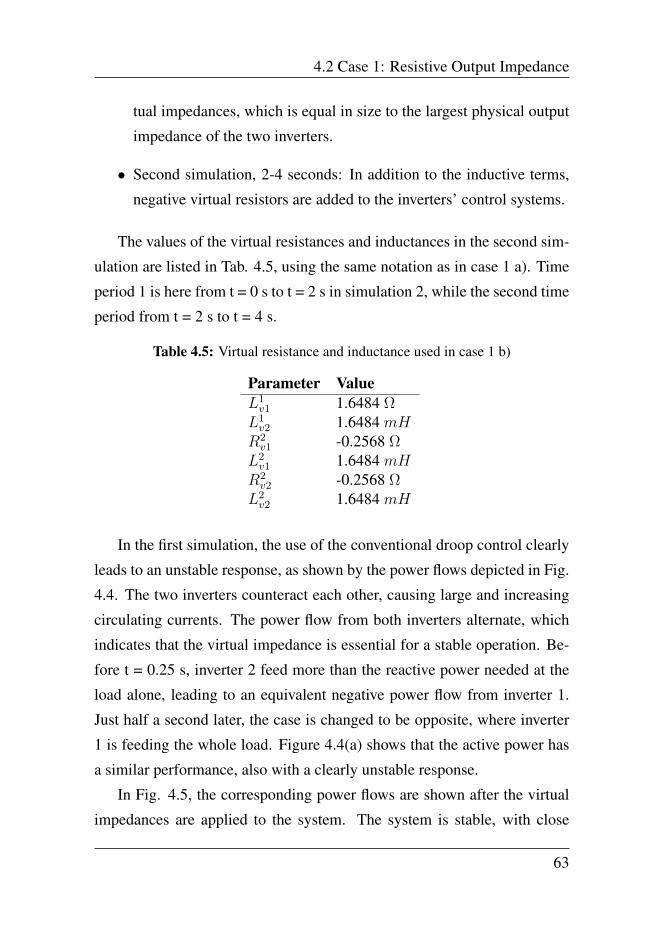
4.2 Case 1: Resistive Output Impedance
tual impedances, which is equal in size to the largest physical output
impedance of the two inverters.
• Second simulation, 2-4 seconds: In addition to the inductive terms,
negative virtual resistors are added to the inverters’ control systems.
The values of the virtual resistances and inductances in the second sim-
ulation are listed in Tab. 4.5, using the same notation as in case 1 a). Time
period 1 is here from t = 0 s to t = 2 s in simulation 2, while the second time
period from t = 2 s to t = 4 s.
Table 4.5: Virtual resistance and inductance used in case 1 b)
Parameter ValueL1v1 1.6484 Ω
L1v2 1.6484 mH
R2v1 -0.2568 Ω
L2v1 1.6484 mH
R2v2 -0.2568 Ω
L2v2 1.6484 mH
In the first simulation, the use of the conventional droop control clearly
leads to an unstable response, as shown by the power flows depicted in Fig.
4.4. The two inverters counteract each other, causing large and increasing
circulating currents. The power flow from both inverters alternate, which
indicates that the virtual impedance is essential for a stable operation. Be-
fore t = 0.25 s, inverter 2 feed more than the reactive power needed at the
load alone, leading to an equivalent negative power flow from inverter 1.
Just half a second later, the case is changed to be opposite, where inverter
1 is feeding the whole load. Figure 4.4(a) shows that the active power has
a similar performance, also with a clearly unstable response.
In Fig. 4.5, the corresponding power flows are shown after the virtual
impedances are applied to the system. The system is stable, with close
63
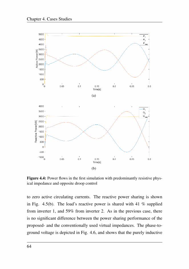
Chapter 4. Cases Studies
(a)
(b)
Figure 4.4: Power flows in the first simulation with predominantly resistive phys-ical impedance and opposite droop control
to zero active circulating currents. The reactive power sharing is shown
in Fig. 4.5(b). The load’s reactive power is shared with 41 % supplied
from inverter 1, and 59% from inverter 2. As in the previous case, there
is no significant difference between the power sharing performance of the
proposed- and the conventionally used virtual impedances. The phase-to-
ground voltage is depicted in Fig. 4.6, and shows that the purely inductive
64

4.2 Case 1: Resistive Output Impedance
(a)
(b)
Figure 4.5: Power flows in the second simulation with predominantly resistivephysical impedance and opposite droop control
virtual impedances cause a voltage drop of around 1 V. By adding negative
resistors to the virtual impedances, the voltage drop is reduced by around
95 %.
65
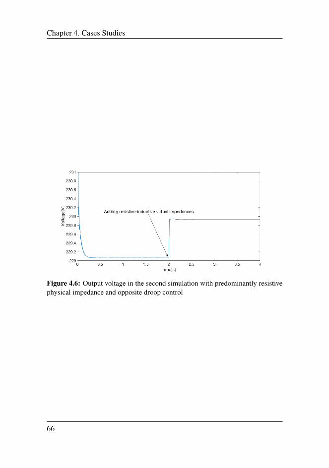
Chapter 4. Cases Studies
Figure 4.6: Output voltage in the second simulation with predominantly resistivephysical impedance and opposite droop control
66

4.3 Case 2: Inductive Output Impedance
4.3 Case 2: Inductive Output Impedance
The output impedance of a microgrid can be dominated by the inductive
behavior of components such as isolating transformers [71]. This is the
case to be studied in this section, by using the conventional droop control in
case 2 a) and the opposite droop control algorithm in case 2 b). A diagram
showing a microgrid system including isolating transformers is depicted in
Fig. 4.7.
Figure 4.7: The investigated system in case 2
The parameters of the distribution lines used in the simulations, in this
case, are based on the simulations from case 1, as explained in Section 2.4.
The physical output impedance is equal as in case 1, but with a contribution
from inductive components the distribution lines are 3-4 times shorter than
in the previous case. The exact physical output impedances used in the
simulations are presented in Tab. 4.6.
67
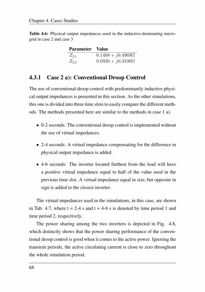
Chapter 4. Cases Studies
Table 4.6: Physical output impedances used in the inductive-dominating micro-grid in case 2 and case 3
Parameter ValueZL1 0.1488 + j0.4969ΩZL2 0.0930 + j0.3100Ω
4.3.1 Case 2 a): Conventional Droop Control
The use of conventional droop control with predominantly inductive physi-
cal output impedances is presented in this section. As the other simulations,
this one is divided into three time slots to easily compare the different meth-
ods. The methods presented here are similar to the methods in case 1 a).
• 0-2 seconds: The conventional droop control is implemented without
the use of virtual impedances.
• 2-4 seconds: A virtual impedance compensating for the difference in
physical output impedance is added.
• 4-6 seconds: The inverter located furthest from the load will have
a positive virtual impedance equal to half of the value used in the
previous time slot. A virtual impedance equal in size, but opposite in
sign is added to the closest inverter.
The virtual impedances used in the simulations, in this case, are shown
in Tab. 4.7, where t = 2-4 s and t = 4-6 s is denoted by time period 1 and
time period 2, respectively.
The power sharing among the two inverters is depicted in Fig. 4.8,
which distinctly shows that the power sharing performance of the conven-
tional droop control is good when it comes to the active power. Ignoring the
transient periods, the active circulating current is close to zero throughout
the whole simulation period.
68
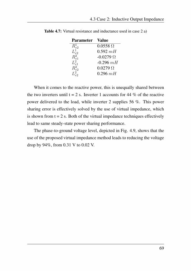
4.3 Case 2: Inductive Output Impedance
Table 4.7: Virtual resistance and inductance used in case 2 a)
Parameter ValueR1v2 0.0558 Ω
L1v2 0.592 mH
R2v1 -0.0279 Ω
L2v1 -0.296 mH
R2v2 0.0279 Ω
L2v2 0.296 mH
When it comes to the reactive power, this is unequally shared between
the two inverters until t = 2 s. Inverter 1 accounts for 44 % of the reactive
power delivered to the load, while inverter 2 supplies 56 %. This power
sharing error is effectively solved by the use of virtual impedance, which
is shown from t = 2 s. Both of the virtual impedance techniques effectively
lead to same steady-state power sharing performance.
The phase-to-ground voltage level, depicted in Fig. 4.9, shows that the
use of the proposed virtual impedance method leads to reducing the voltage
drop by 94%, from 0.31 V to 0.02 V.
69
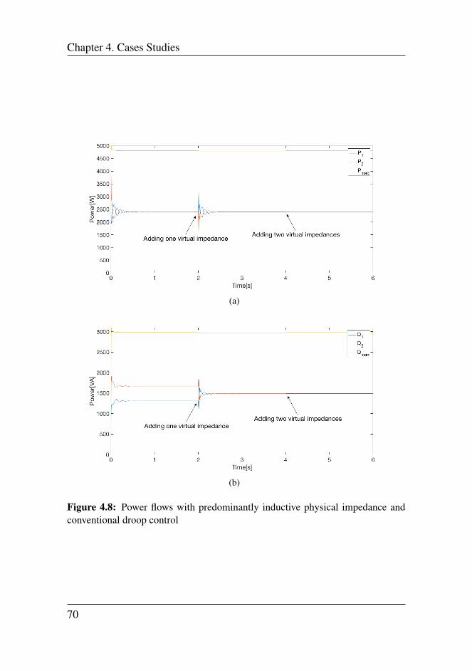
Chapter 4. Cases Studies
(a)
(b)
Figure 4.8: Power flows with predominantly inductive physical impedance andconventional droop control
70
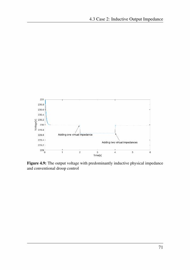
4.3 Case 2: Inductive Output Impedance
Figure 4.9: The output voltage with predominantly inductive physical impedanceand conventional droop control
71
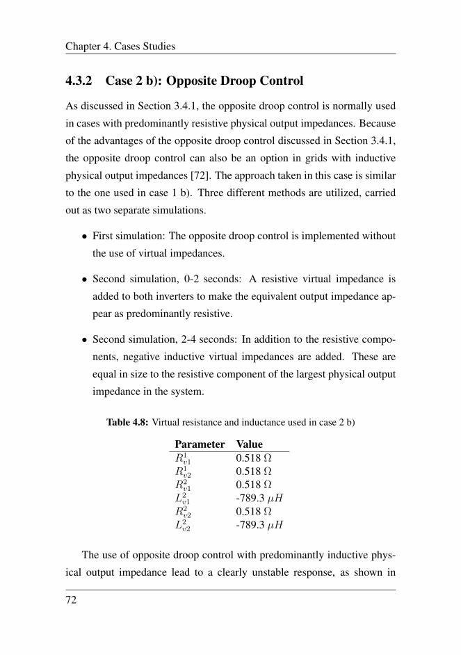
Chapter 4. Cases Studies
4.3.2 Case 2 b): Opposite Droop Control
As discussed in Section 3.4.1, the opposite droop control is normally used
in cases with predominantly resistive physical output impedances. Because
of the advantages of the opposite droop control discussed in Section 3.4.1,
the opposite droop control can also be an option in grids with inductive
physical output impedances [72]. The approach taken in this case is similar
to the one used in case 1 b). Three different methods are utilized, carried
out as two separate simulations.
• First simulation: The opposite droop control is implemented without
the use of virtual impedances.
• Second simulation, 0-2 seconds: A resistive virtual impedance is
added to both inverters to make the equivalent output impedance ap-
pear as predominantly resistive.
• Second simulation, 2-4 seconds: In addition to the resistive compo-
nents, negative inductive virtual impedances are added. These are
equal in size to the resistive component of the largest physical output
impedance in the system.
Table 4.8: Virtual resistance and inductance used in case 2 b)
Parameter ValueR1v1 0.518 Ω
R1v2 0.518 Ω
R2v1 0.518 Ω
L2v1 -789.3 µH
R2v2 0.518 Ω
L2v2 -789.3 µH
The use of opposite droop control with predominantly inductive phys-
ical output impedance lead to a clearly unstable response, as shown in
72
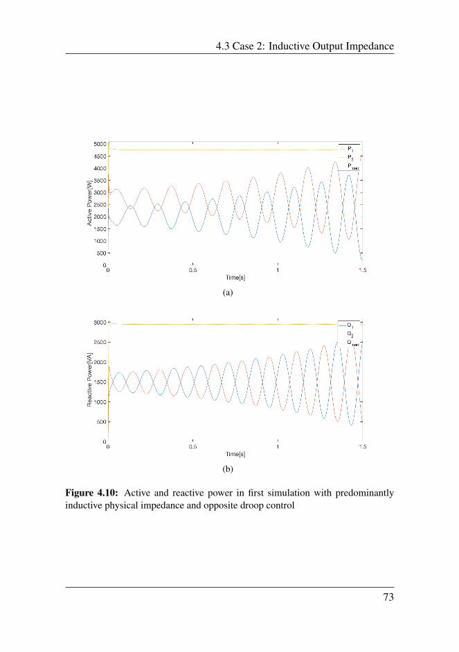
4.3 Case 2: Inductive Output Impedance
(a)
(b)
Figure 4.10: Active and reactive power in first simulation with predominantlyinductive physical impedance and opposite droop control
73
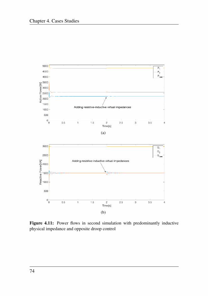
Chapter 4. Cases Studies
(a)
(b)
Figure 4.11: Power flows in second simulation with predominantly inductivephysical impedance and opposite droop control
74
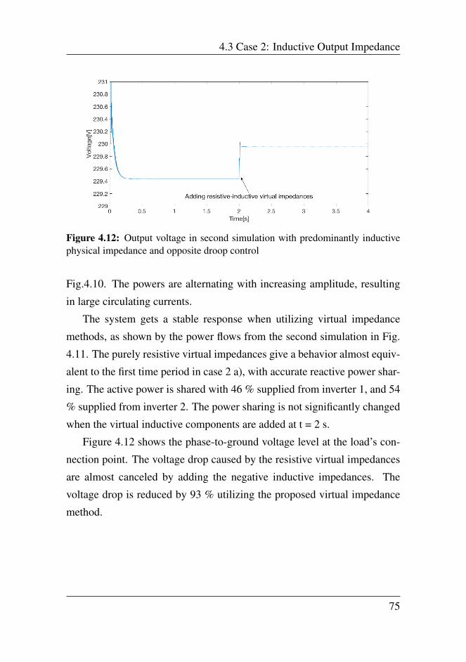
4.3 Case 2: Inductive Output Impedance
Figure 4.12: Output voltage in second simulation with predominantly inductivephysical impedance and opposite droop control
Fig.4.10. The powers are alternating with increasing amplitude, resulting
in large circulating currents.
The system gets a stable response when utilizing virtual impedance
methods, as shown by the power flows from the second simulation in Fig.
4.11. The purely resistive virtual impedances give a behavior almost equiv-
alent to the first time period in case 2 a), with accurate reactive power shar-
ing. The active power is shared with 46 % supplied from inverter 1, and 54
% supplied from inverter 2. The power sharing is not significantly changed
when the virtual inductive components are added at t = 2 s.
Figure 4.12 shows the phase-to-ground voltage level at the load’s con-
nection point. The voltage drop caused by the resistive virtual impedances
are almost canceled by adding the negative inductive impedances. The
voltage drop is reduced by 93 % utilizing the proposed virtual impedance
method.
75

Chapter 4. Cases Studies
4.4 Case 3: Estimated Inductive Output Impedance
In the previous cases, the inverters’ physical output impedance are assumed
to be known. In an actual microgrid, this is normally not the case. This case
considers the same cases as those including virtual impedances in case 2.
The physical output impedances of the inverters are estimated 25 % lower
than the actual values. Since the virtual impedances are selected based on
the physical output impedances, the estimations affect their values. The
other parameters used in the simulations in this case are the same as in
case 2. The physical output impedances are given by Tab. 4.6.
4.4.1 Case 3 a): Conventional Droop Control
This case is a reproduction of case 2 a), with use of conventional droop con-
trol with predominantly inductive physical output impedances. The simu-
lation is divided into three time slots, as in case 2 a).
• 0-2 seconds: The conventional droop control is implemented without
use of virtual impedances.
• 2-4 seconds: A virtual impedance compensating for the difference in
physical output impedance is added.
• 4-6 seconds: The inverter located furthest from the load will have
a positive virtual impedance equal to half of the value used in the
previous time slot. A virtual impedance equal in size, but opposite in
sign is added to the closest inverter.
The physical output impedances are assumed to be estimated to be 75
% of the actual physical output impedances. Since the estimated physi-
cal output impedances are used to select the virtual impedances, the vir-
tual impedances in this case are 25 % lower than in case 2 a). The virtual
76

4.4 Case 3: Estimated Inductive Output Impedance
impedances used are shown in Tab. 4.9, where the time periods t = 2-4 s
and t = 4-6 s are denoted by time period 1 and time period 2, respectively.
Table 4.9: Virtual resistance and inductance used in case 3 a)
Parameter ValueR1v2 0.0418 Ω
L1v2 0.440 mH
R2v1 -0.0209 Ω
L2v1 -0.220 mH
R2v2 0.0209 Ω
L2v2 0.220 mH
The power flows from the two inverters are depicted in Fig. 4.13. This
figure shows that with 25 % error in the physical output impedance estima-
tions, the effect of the virtual impedances is similar to case 2 a), but with
relatively small reactive circulating currents. The power sharing with the
conventionally used and the proposed virtual impedance method is effec-
tively equal, as shown in Fig. 4.13. The active power is shared equally
among the inverters. With known physical output impedances in case 2 a),
the virtual impedances provided almost perfect compensation, resulting in
approximately zero circulating currents when they where applied to the sys-
tem. In this case, a small circulating current appears, where inverter 1 feeds
around 48 % of the reactive power, while inverter 2 delivers the remaining
52 %.
In Fig. 4.14, the load’s phase-to-ground voltage is shown, which is
similar to the voltage level in case 2 a). The voltage drop related to the
virtual impedance is reduced by around 91 % by using the proposed vir-
tual impedance method, which is slightly less than in the case with known
physical output impedances.
77
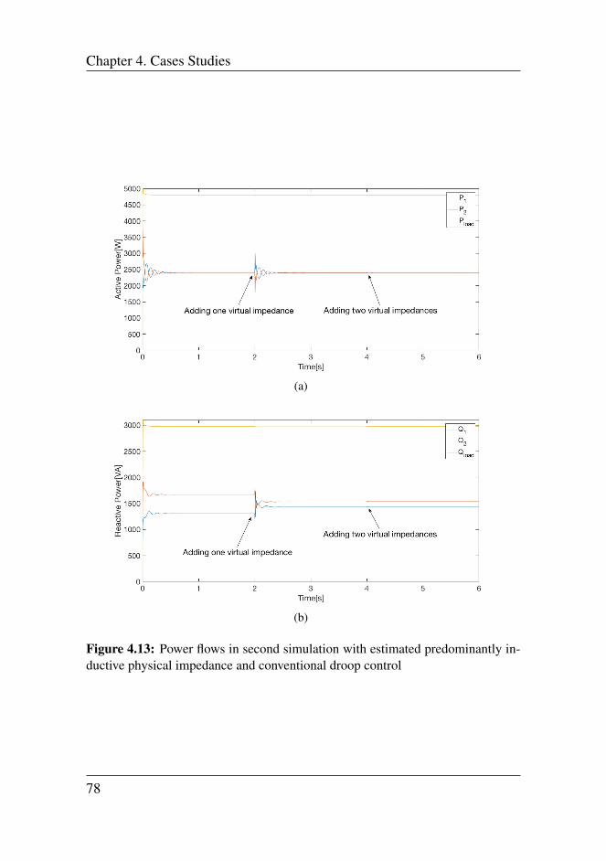
Chapter 4. Cases Studies
(a)
(b)
Figure 4.13: Power flows in second simulation with estimated predominantly in-ductive physical impedance and conventional droop control
78

4.4 Case 3: Estimated Inductive Output Impedance
Figure 4.14: Output voltage with estimated inductive physical impedance andconventional droop control
79
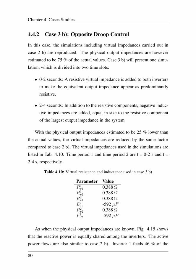
Chapter 4. Cases Studies
4.4.2 Case 3 b): Opposite Droop Control
In this case, the simulations including virtual impedances carried out in
case 2 b) are reproduced. The physical output impedances are however
estimated to be 75 % of the actual values. Case 3 b) will present one simu-
lation, which is divided into two time slots:
• 0-2 seconds: A resistive virtual impedance is added to both inverters
to make the equivalent output impedance appear as predominantly
resistive.
• 2-4 seconds: In addition to the resistive components, negative induc-
tive impedances are added, equal in size to the resistive component
of the largest output impedance in the system.
With the physical output impedances estimated to be 25 % lower than
the actual values, the virtual impedances are reduced by the same factor
compared to case 2 b). The virtual impedances used in the simulations are
listed in Tab. 4.10. Time period 1 and time period 2 are t = 0-2 s and t =
2-4 s, respectively.
Table 4.10: Virtual resistance and inductance used in case 3 b)
Parameter ValueR1v1 0.388 Ω
R1v2 0.388 Ω
R2v1 0.388 Ω
L2v1 -592 µF
R2v2 0.388 Ω
L2v2 -592 µF
As when the physical output impedances are known, Fig. 4.15 shows
that the reactive power is equally shared among the inverters. The active
power flows are also similar to case 2 b). Inverter 1 feeds 46 % of the
80
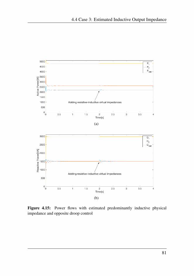
4.4 Case 3: Estimated Inductive Output Impedance
(a)
(b)
Figure 4.15: Power flows with estimated predominantly inductive physicalimpedance and opposite droop control
81

Chapter 4. Cases Studies
Figure 4.16: Output voltage with estimated inductive physical impedance andopposite droop control
load’s active power, while inverter 2 delivers 56 %. The circulating current
is slightly larger than with known physical output impedances.
The load’s phase-to-ground voltage level is shown in Fig. 4.16. With
the proposed virtual impedance method, the voltage drop due to the virtual
impedances is reduced by 95 % compared to the purely resistive virtual
impedance.
82
4.5 Discussion
4.5 Discussion
The islanded microgrid system is implemented and tested through different
case studies. The simulations show that the use of virtual impedances im-
proves the power sharing among inverters. The proposed virtual impedance
methods have the same power sharing performance as existing methods, but
the voltage drop across the virtual impedances are significantly reduced. In
this section, simplifications and possible improvements related to the mi-
crogrid systems are discussed.
The case studies has shown how virtual impedances are used to improve
power sharing among paralleled inverters. A presentation of proposed vir-
tual impedance methods are done, where the methods aim for sufficient
power sharing, with less effect on the output voltage. Virtual impedance
methods are proposed in six different cases. The simulation results show
that for all cases, the proposed methods achieve at least 90 % reduced volt-
age drop compared to existing virtual impedance solutions. By using the
proposed approaches, a larger portion of the power sharing control can be
moved from the centralized to the distributed control. With a negligible
voltage drop caused by the virtual impedances, the droop controller’s volt-
age reference does not have to be changed because of a load shift, which
can have been the case when using the existing virtual impedance methods.
A disadvantage of the proposed method utilized in case 1 a), 2 a) and 3
a), is that the method is dependent on having an even number of inverters,
since the virtual impedances are implemented as pairs. Each inverter with
a positive virtual impedance should always have another inverter with the
same virtual impedance, but with opposite sign. This method may therefore
face challenges when having an odd number of inverters.
Another scenario, which will be challenging both when using the
conventional and the proposed virtual impedance method used in case 1 a),
83

Chapter 4. Cases Studies
2 a) and 3 a), is to have loads connected at several locations in the micro-
grid. In real life, this would normally be the case. With several loads at dif-
ferent locations in the grid, both the existing- and the proposed impedance
matching technique used in case 1 a), 2 a) and 3 a) will have a significant
reduction in power sharing performance. Utilization of both the impedance
matching techniques presented in this thesis can possibly lead to unstable
behavior in a microgrid with several connection points for loads.
The second proposed method, which is utilized in case 1 b), 2 b) and
3 b), may experience challenges related to the selection of the negative
component of the virtual impedances. When the method is applied to the
conventional droop control method, the virtual impedance will have a pos-
itive inductive and a negative resistive component. If the resistive value is
selected too large, it can possibly compensate for all of the resistive effects
in the physical output impedance. The equivalent output impedances of the
inverters will appear as purely inductive. As discussed in Section 3.4.1,
a purely inductive output impedance would lead to an unstable behavior,
because of no damping effect which is normally utilized by the resistive
components [9, chapter 3].
When modelling the microgrid systems, simplifications have been done.
One of the largest is the use of the average model VSIs. This inverter model
does not produce harmonic oscillations or take inverter losses into consider-
ation. Due to this simplification, harmonic power sharing is not considered.
The advantage of the average model is mainly related to the computational
time when doing simulations, where this model allows the step size to be
larger than alternative methods does. Because of the reduced computational
time, this model is preferred instead of more accurate models.
Another simplification is related to the representation of the DG units.
They are modelled as ideal dc voltage sources, and are therefore assumed
to have an infinite amount of available power. The assumption is done on
84
4.5 Discussion
the background of this work’s main goal, which is focused on studying
the power sharing performance for inverters with different physical output
impedances. The use of dc voltage sources is for this purpose considered as
good enough, since it is focused on the steady-state performance. Most of
the reviewed publications focused on power sharing also use this assump-
tion. In a more complete study, the DG units could have been represented
with fluctuating power production. In addition, batteries could have been
considered to be both charged and discharged, depending on the production
and loads in the system.
When considering the simulation results, there are several aspects that
should be mentioned. The voltage drops caused by the virtual impedances
used in the case studies are relatively small, maximum 1 V. Thus, the pro-
posed methods can be more valuable in a grid with a larger load, which
will have a larger voltage drop considering the same voltage level. Since
the microgrid feeds a single residential load, a system including a larger
load is seen as realistic.
In all the simulations, the parameters of the distribution lines and other
components in the grid are assumed to be known, which implies that the
physical output impedance is known. This is rarely the case in a real life
microgrid, where the parameters often have to be estimated, for instance by
using standard values as in Tab. 2.2 [9, chapter 3]. Simulation case 3 is a
reproduction of simulation case 2, but the physical output impedances are
estimated to be 25 % below the actual values. This is considered as a rela-
tively large error. The results from the two cases are however similar, with
only slightly larger circulating currents in case 3. The voltage drops from
the virtual impedances are significantly reduced, both in case 3 a) and b).
The results thereby show that the virtual impedance methods seem to work
also with roughly estimated line impedances, but with a slightly reduced
power sharing performance. The proposed virtual impedance methods uti-
85
Chapter 4. Cases Studies
lized show an improved behavior compared to the more conventional vir-
tual impedance methods, also in case 3. The two methods provide the same
power sharing performance, but the proposed virtual impedance method
has an improved voltage level compared to the more conventional virtual
impedance method.
The lengths of the predominantly resistive distribution lines used in case
1 are selected to be 500m and 800m. This is considered to be a reasonable
difference between the inverters, but also reasonable lengths, relative to the
voltage level and the size of the load. With much longer distribution lines,
the voltage level of the power system will probably be considered increased,
in order to reduce transmission losses [73, chapter 2]. With predominantly
inductive physical output impedance in case 2 and 3, the lengths of the dis-
tribution lines are assumed to be shorter than in case 1. If the lengths of the
lines are increased, it would cause a decreased X/R-ratio, since the distribu-
tion lines’ impedance will amount to a larger portion of the physical output
impedance of the inverters. This would increase the coupling between ac-
tive and reactive power, which may lead to new requirements, for instance
in the selection of the virtual impedances.
This study presents promising results, but should be considered as a
preliminary study within the use of virtual impedance for power sharing
purposes. The results are carried out based on one specific system, which
is based on two ideal inverter-based generation units.
As mentioned, a set of limitations is related to the study. Further in-
vestigation should be done, reducing the number of limitations in order to
achieve a more complete analysis. Even though there is a need for more
research on the topic, it should be noticed that the proposed methods in this
thesis achieve improved voltage level without reducing the power sharing
performance, compared to the more conventional virtual impedance meth-
ods. This utilization of virtual impedance in the distributed control may
86
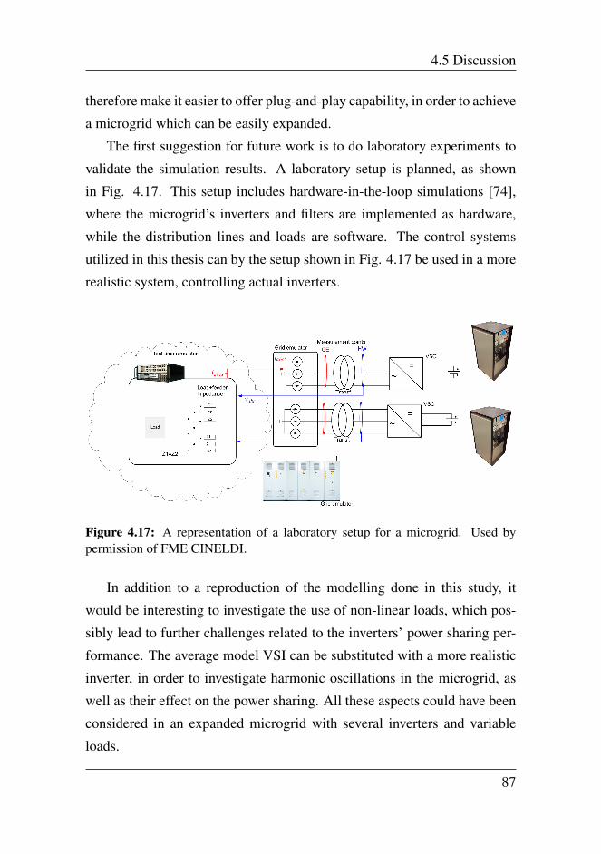
4.5 Discussion
therefore make it easier to offer plug-and-play capability, in order to achieve
a microgrid which can be easily expanded.
The first suggestion for future work is to do laboratory experiments to
validate the simulation results. A laboratory setup is planned, as shown
in Fig. 4.17. This setup includes hardware-in-the-loop simulations [74],
where the microgrid’s inverters and filters are implemented as hardware,
while the distribution lines and loads are software. The control systems
utilized in this thesis can by the setup shown in Fig. 4.17 be used in a more
realistic system, controlling actual inverters.
Figure 4.17: A representation of a laboratory setup for a microgrid. Used bypermission of FME CINELDI.
In addition to a reproduction of the modelling done in this study, it
would be interesting to investigate the use of non-linear loads, which pos-
sibly lead to further challenges related to the inverters’ power sharing per-
formance. The average model VSI can be substituted with a more realistic
inverter, in order to investigate harmonic oscillations in the microgrid, as
well as their effect on the power sharing. All these aspects could have been
considered in an expanded microgrid with several inverters and variable
loads.
87

Chapter 4. Cases Studies
88

5 | Conclusion
An islanded microgrid system is modelled in order to investigate power
sharing between paralleled DG units with different output impedances. In
the studied system, two DG units connected through inverters are modelled
to feed one linear load. This thesis shows the distributed control structure,
including the inner- and primary control. The inner control includes volt-
age and current control, while the primary control contains a droop con-
trol algorithm which takes care of voltage and frequency levels. In this
loop, the output impedances of the inverters are modified by use of vir-
tual impedances, which contribute to improved power sharing among the
inverters. Six different cases are considered, and it is investigated how vir-
tual impedance can be used to utilize different control systems in grids with
mismatching physical output impedances. The system is validated through
simulations, divided into three main cases.
Case 1 represents the microgrid system with predominantly resistive
physical output impedances. Two different droop control algorithms, con-
ventional and opposite droop control, are considered. In order to improve
power sharing, the effectiveness of virtual impedances is validated through
simulations. Proposed solutions show how virtual impedances can be used
with power sharing performance similar to the conventional methods. The
voltage drops due to the virtual impedances are however significantly re-
duced by utilizing these solutions.
89
In case 2, predominantly inductive physical output impedances are stud-
ied. The same droop control methods are used, and virtual impedance tech-
niques are utilized. As in case 1, existing virtual impedance methods are
validated, including proposed solutions with less effect on the voltage lev-
els. The proposed solutions lead to reduced voltage drops, and the power
sharing performance is practically the same as for the already existing vir-
tual impedance methods.
In simulation case 3, it is shown that with predominantly inductive
physical output impedance roughly estimated, virtual impedance methods
can improve the power sharing. At the same time, only small voltage drops
are experienced across the proposed virtual impedances. The power shar-
ing performance is however reduced compared to the ideal case, where the
physical output impedances are known.
This thesis presents promising results, where virtual impedance meth-
ods show well-working power sharing performance, in addition to minor
effects on the output voltage level. The results should still be seen as a
preliminary study, due to the assumptions that are done. For further work,
it is suggested to perform laboratory experiments in order to validate the
simulations in a more realistic sceanario. In addition, expansions of the
microgrid, the use of non-linear loads and inclusion of more application
oriented simulations can be part of future research on the topic of power
sharing in islanded ac microgrids.
90

Bibliography
[1] Joan Rocabert, Alvaro Luna, Frede Blaabjerg, and Pedro Rodriguez.
Control of power converters in ac microgrids. IEEE transactions on
power electronics, 27(11):4734–4749, 2012.
[2] The paris agreement - status of ratification. http://unfccc.
int/paris_agreement/items/9444.php. Accessed: 2018-
12-03.
[3] The paris agreement. http://unfccc.int/paris_
agreement/items/9485.php. Accessed: 2018-12-03.
[4] The impact of population momentum on future population growth.
https://esa.un.org/unpd/wpp/Publications/
Files/PopFacts_2017-4_Population-Momentum.pdf.
Accessed: 2018-12-03.
[5] Renewable energy: A key climate solution. https:
//www.irena.org/-/media/Files/IRENA/
Agency/Publication/2017/Nov/IRENA_A_key_
climate_solution_2017.pdf?la=en&hash=
A9561C1518629886361D12EFA11A051E004C5C98. Ac-
cessed: 2018-24-05.
91
[6] Daniel E Olivares, Ali Mehrizi-Sani, Amir H Etemadi, Claudio A
Cañizares, Reza Iravani, Mehrdad Kazerani, Amir H Hajimiragha,
Oriol Gomis-Bellmunt, Maryam Saeedifard, Rodrigo Palma-Behnke,
et al. Trends in microgrid control. IEEE Transactions on smart grid,
5(4):1905–1919, 2014.
[7] Key world energy statistics. https://www.iea.org/
publications/freepublications/publication/
KeyWorld2017.pdf. Accessed: 2017-12-17.
[8] Renewablles 2016: Global status report. http://www.ren21.
net/wp-content/uploads/2016/06/GSR_2016_Full_
Report.pdf. Accessed: 2018-24-05.
[9] Nikos Hatziargyriou et al. Microgrids: architectures and control. Wi-
ley Online Library, 2014.
[10] SM Shinde, KD Patil, SS Khairnar, and WZ Gandhare. The role of
power electronics in renewable energy systems research and develop-
ment. In Emerging Trends in Engineering and Technology (ICETET),
2009 2nd International Conference on, pages 726–730. IEEE, 2009.
[11] Ching-Tsai Pan and Yi-Hung Liao. Modeling and coordinate control
of circulating currents in parallel three-phase boost rectifiers. IEEE
Transactions on Industrial Electronics, 54(2):825–838, 2007.
[12] Santiago Grijalva and Muhammad Umer Tariq. Prosumer-based smart
grid architecture enables a flat, sustainable electricity industry. In
Innovative Smart Grid Technologies (ISGT), 2011 IEEE PES, pages
1–6. IEEE, 2011.
[13] About microgrids. http://www.microgridinstitute.
org/about-microgrids.html. Accessed: 2018-10-04.
92

[14] Robert H Lasseter. Microgrids. In Power Engineering Society Winter
Meeting, 2002. IEEE, volume 1, pages 305–308. IEEE, 2002.
[15] Joan Rocabert, Alvaro Luna, Frede Blaabjerg, and Pedro Rodriguez.
Control of power converters in ac microgrids. IEEE transactions on
power electronics, 27(11):4734–4749, 2012.
[16] Farid Katiraei, Reza Iravani, Nikos Hatziargyriou, and Aris Dimeas.
Microgrids management. IEEE power and energy magazine, 6(3),
2008.
[17] Hua Han, Xiaochao Hou, Jian Yang, Jifa Wu, Mei Su, and Josep M
Guerrero. Review of power sharing control strategies for islanding op-
eration of ac microgrids. IEEE Transactions on Smart Grid, 7(1):200–
215, 2016.
[18] TL Vandoorn, JM Guerrero, JDM De Kooning, J Vásquez, and L Van-
develde. Decentralized and centralized control of islanded microgrids
including reserve management. IEEE Ind Electron Mag, pages 1–14,
2013.
[19] Anders Bergheim Holvik. Control of power electronics in microgrids,
2017.
[20] Stavros Papathanassiou, Nikos Hatziargyriou, Kai Strunz, et al. A
benchmark low voltage microgrid network. In Proceedings of the
CIGRE symposium: power systems with dispersed generation, pages
1–8, 2005.
[21] Yasser Mohamed. New control algorithms for the distributed genera-
tion interface in grid-connected and micro-grid systems. 2008.
93

[22] Mohammad Hadi Andishgar, Eskandar Gholipour, and Rahmat-allah
Hooshmand. An overview of control approaches of inverter-based mi-
crogrids in islanding mode of operation. Renewable and Sustainable
Energy Reviews, 80:1043–1060, 2017.
[23] Jan Bauer, Jiri Lettl, Petr Pichlik, and Jiri Zdenek. Low power photo-
voltaic converter control and development. Transactions on Electrical
Engineering, 1(3), 2012.
[24] Utsav P Yagnik and Mehul D Solanki. Comparison of l, lc & lcl filter
for grid connected converter. In Trends in Electronics and Informat-
ics (ICEI), 2017 International Conference on, pages 455–458. IEEE,
2017.
[25] Vegard Moritsgård Flatjord. Active filter capability of a voltage source
inverter in marine applications. Master’s thesis, NTNU, 2017.
[26] Anca Julean. Active damping of lcl filter resonance in grid con-
nected applications. Aalborg Universitet, Dinamarca, Dissertação de
mestrado, 2009.
[27] Hisham Mahmood, Dennis Michaelson, and Jin Jiang. Accurate re-
active power sharing in an islanded microgrid using adaptive virtual
impedances. IEEE Transactions on Power Electronics, 30(3):1605–
1617, 2015.
[28] Ned Mohan, Tore Undeland, and William P. Robbins. Power elec-
tronics: converters, applications, and design. John Wiley & Sons,
3rd edition, 2003.
[29] Temesgen Mulugeta Haileselassie. Control, dynamics and operation
of multi-terminal vsc-hvdc transmission systems. 2012.
94
[30] Technical guide specifications power wave 3. https://www.
onlinepower.com/pdf/powerwave3_TS.pdf. Accessed:
2018-30-05.
[31] Universal bridge. https://se.mathworks.com/help/
physmod/sps/powersys/ref/universalbridge.html.
Accessed: 2017-12-02.
[32] Zhongming Ye, Praveen K Jain, and Paresh C Sen. Circulating cur-
rent minimization in high-frequency ac power distribution architec-
ture with multiple inverter modules operated in parallel. IEEE Trans-
actions on Industrial Electronics, 54(5):2673–2687, 2007.
[33] Ching-Tsai Pan and Yi-Hung Liao. Modeling and control of circulat-
ing currents for parallel three-phase boost rectifiers with different load
sharing. IEEE Transactions on Industrial Electronics, 55(7):2776–
2785, 2008.
[34] Wei Yao, Min Chen, José Matas, Josep M Guerrero, and Zhao-Ming
Qian. Design and analysis of the droop control method for paral-
lel inverters considering the impact of the complex impedance on
the power sharing. IEEE Transactions on Industrial Electronics,
58(2):576–588, 2011.
[35] Xiongfei Wang, Frede Blaabjerg, and Zhe Chen. An improved design
of virtual output impedance loop for droop-controlled parallel three-
phase voltage source inverters. In Energy Conversion Congress and
Exposition (ECCE), 2012 IEEE, pages 2466–2473. IEEE, 2012.
[36] Usman Bashir Tayab, Mohd Azrik Bin Roslan, Leong Jenn Hwai,
and Muhammad Kashif. A review of droop control techniques for
95
microgrid. Renewable and Sustainable Energy Reviews, 76:717–727,
2017.
[37] Prasenjit Basak, S Chowdhury, S Halder nee Dey, and SP Chowdhury.
A literature review on integration of distributed energy resources in
the perspective of control, protection and stability of microgrid. Re-
newable and Sustainable Energy Reviews, 16(8):5545–5556, 2012.
[38] Josep M Guerrero, Juan C Vasquez, José Matas, Luis García
De Vicuña, and Miguel Castilla. Hierarchical control of droop-
controlled ac and dc microgrids—a general approach toward standard-
ization. IEEE Transactions on Industrial Electronics, 58(1):158–172,
2011.
[39] K De Brabandere, B Bolsens, J Van den Keybus, A Woyte, J Driesen,
R Belmans, and K U Leuven. A voltage and frequency droop control
method for parallel inverters. Power Electronics Specialists Confer-
ence, 2004. PESC 04. 2004 IEEE 35th Annual, 4(4):2501–2507 Vol.4,
2004.
[40] Azziddin M Razali, M Azizur Rahman, and Nasrudin A Rahim. Im-
plementation of dq decoupling and feed-forward current controller
for grid connected three phase voltage source converter. In Industry
Applications Society Annual Meeting, 2014 IEEE, pages 1–8. IEEE,
2014.
[41] Jens G Balchen, Trond Andresen, and Bjarne A. Foss. Regulering-
steknikk. Institutt for Teknisk Kybernetikk, NTNU, 2003.
[42] Ned Mohan. Advanced electric drives: analysis, control and model-
ing using MATLAB/Simulink. Wiley, 2014.
96
[43] Roy Nilsen. Tet4120 electric drives. Department of Electrical Engi-
neering, NTNU, Trondheim, 2016.
[44] Ned Mohan. Electric machines and drives: a first course. John Wiles
& Sons, 2012.
[45] Santiago Sanchez, Gilbert Bergna, and Elisabetta Tedeschi. Tuning of
control loops for grid-connected modular multilevel converters under
a simplified port representation for large system studies. In Ecological
Vehicles and Renewable Energies (EVER), 2017 Twelfth International
Conference on, pages 1–8. IEEE, 2017.
[46] Jan Machowski, Janusz W. Bialek, and James R. Bumby. Power Sys-
tem Dynamics. Stability and Control. John Wiley & Sons, 2nd edition,
2014.
[47] Lianqing Zheng, Chen Zhuang, Jian Zhang, and Xiong Du. An en-
hanced droop control scheme for islanded microgrids. International
Journal of Control and Automation, 8(4):63–74, 2015.
[48] Qing-Chang Zhong and Yu Zeng. Can the output impedance of an in-
verter be designed capacitive? In IECON 2011-37th Annual Confer-
ence on IEEE Industrial Electronics Society, pages 1220–1225. IEEE,
2011.
[49] Alexander Micallef, Maurice Apap, Cyril Spiteri-Staines, Josep M
Guerrero, and Juan C Vasquez. Reactive power sharing and voltage
harmonic distortion compensation of droop controlled single phase
islanded microgrids. IEEE Transactions on Smart Grid, 5(3):1149–
1158, 2014.
[50] Alexandra Von Meier. Electric power systems: a conceptual intro-
duction. John Wiley & Sons, 2006.
97
[51] Islam Ziouani, Djamel Boukhetala, Abdel-Moumen Darcherif, Bilal
Amghar, and Ikram El Abbassi. Hierarchical control for flexible mi-
crogrid based on three-phase voltage source inverters operated in par-
allel. International Journal of Electrical Power & Energy Systems,
95:188–201, 2018.
[52] Alfred Engler and Nikos Soultanis. Droop control in lv-grids. In
Future Power Systems, 2005 International Conference on, pages 6–
pp. IEEE, 2005.
[53] Guzman Diaz, Cristina Gonzalez-Moran, Javier Gomez-Aleixandre,
and Alberto Diez. Scheduling of droop coefficients for frequency
and voltage regulation in isolated microgrids. IEEE Transactions on
Power Systems, 25(1):489–496, 2010.
[54] Xiaochao Hou, Yao Sun, Wenbin Yuan, Hua Han, Chaolu Zhong, and
Josep M Guerrero. Conventional p-ω/qv droop control in highly re-
sistive line of low-voltage converter-based ac microgrid. Energies,
9(11):943, 2016.
[55] Yasser Abdel-Rady Ibrahim Mohamed and Ehab F El-Saadany. Adap-
tive decentralized droop controller to preserve power sharing stabil-
ity of paralleled inverters in distributed generation microgrids. IEEE
Transactions on Power Electronics, 23(6):2806–2816, 2008.
[56] Josep M Guerrero, José Matas, Luis Garcia de Vicuna, Miguel
Castilla, and Jaume Miret. Decentralized control for parallel operation
of distributed generation inverters using resistive output impedance.
IEEE Transactions on industrial electronics, 54(2):994–1004, 2007.
[57] Estefanía Planas, Asier Gil-de Muro, Jon Andreu, Iñigo Kortabarria,
and Iñigo Martínez de Alegría. General aspects, hierarchical controls
98

and droop methods in microgrids: A review. Renewable and Sustain-
able Energy Reviews, 17:147–159, 2013.
[58] Ping Zhang, Hengyang Zhao, Huanyu Cai, Jianjiang Shi, and Xiangn-
ing He. Power decoupling strategy based on virtual negative resis-
tor for inverters in low-voltage microgrids. IET Power Electronics,
9(5):1037–1044, 2016.
[59] Yun Wei Li and Ching-Nan Kao. An accurate power control strategy
for power-electronics-interfaced distributed generation units operat-
ing in a low-voltage multibus microgrid. IEEE Transactions on Power
Electronics, 24(12):2977–2988, 2009.
[60] Meng Chen and Xiangning Xiao. Hierarchical frequency control strat-
egy of hybrid droop/vsg-based islanded microgrids. Electric Power
Systems Research, 155:131–143, 2018.
[61] Andrew D Paquette and Deepak M Divan. Virtual impedance cur-
rent limiting for inverters in microgrids with synchronous generators.
IEEE Transactions on Industry Applications, 51(2):1630–1638, 2015.
[62] Apap M. Micallef, A. and C. Spiteri-Staines. Performance compar-
ison for virtual impedance techniques used in droop controlled is-
landed microgrids. International Symposium on Power Electronics,
pages 695–700, 2016.
[63] Xiongfei Wang, Yun Wei Li, Frede Blaabjerg, and Poh Chi-
ang Loh. Virtual-impedance-based control for voltage-source and
current-source converters. IEEE Transactions on Power Electronics,
30(12):7019–7037, 2015.
99

[64] Xiangyu Wu, Chen Shen, and Reza Iravani. Feasible range and opti-
mal value of the virtual impedance for droop-based control of micro-
grids. IEEE Transactions on Smart Grid, 8(3):1242–1251, 2017.
[65] Herong Gu, Deyu Wang, Hong Shen, Wei Zhao, and Xiaoqiang Guo.
New power sharing control for inverter-dominated microgrid based on
impedance match concept. The Scientific World Journal, 2013, 2013.
[66] Jianjun Su, Jieyun Zheng, Demin Cui, Xiaobo Li, Zhijian Hu, and
Chengxue Zhang. An integrated control strategy adopting droop con-
trol with virtual inductance in microgrid. Engineering, 5(01):44,
2013.
[67] Jinwei He and Yun Wei Li. Analysis, design, and implementation of
virtual impedance for power electronics interfaced distributed genera-
tion. IEEE Transactions on Industry Applications, 47(6):2525–2538,
2011.
[68] TL Vandoorn, JDM De Kooning, Bart Meersman, and Lieven Van-
develde. Improvement of active power sharing ratio of p/v droop
controllers in low-voltage islanded microgrids. In Power and Energy
Society General Meeting (PES), 2013 IEEE, pages 1–5. IEEE, 2013.
[69] Jinwei He, Yun Wei Li, Josep M Guerrero, Frede Blaabjerg, and
Juan C Vasquez. An islanding microgrid power sharing approach us-
ing enhanced virtual impedance control scheme. IEEE Transactions
on Power Electronics, 28(11):5272–5282, 2013.
[70] The national smart grid laboratory. https://www.ntnu.edu/
smartgrid. Accessed: 2017-12-16.
[71] Zhikang Shuai, MO Shanglin, WANG Jun, Z John Shen, TIAN Wei,
and FENG Yan. Droop control method for load share and voltage reg-
100
ulation in high-voltage microgrids. Journal of Modern Power Systems
and Clean Energy, 4(1):76–86, 2016.
[72] SLS Lima, RFS Dias, and EH Watanabe. Indirect voltage control (ivc)
versus direct voltage control (dvc) in distribution grids with renew-
able energy sources. In Power Electronics for Distributed Generation
Systems (PEDG), 2017 IEEE 8th International Symposium on, pages
1–6. IEEE, 2017.
[73] Stephen Chapman. Electric machinery fundamentals. Tata McGraw-
Hill Education, 2005.
[74] What is hardware-in-the-loop simulation? https:
//se.mathworks.com/help/physmod/simscape/ug/
what-is-hardware-in-the-loop-simulation.html.
Accessed: 2017-12-17.
[75] Robert H Park. Two-reaction theory of synchronous machines gener-
alized method of analysis-part i. Transactions of the American Insti-
tute of Electrical Engineers, 48(3):716–727, 1929.
101

102
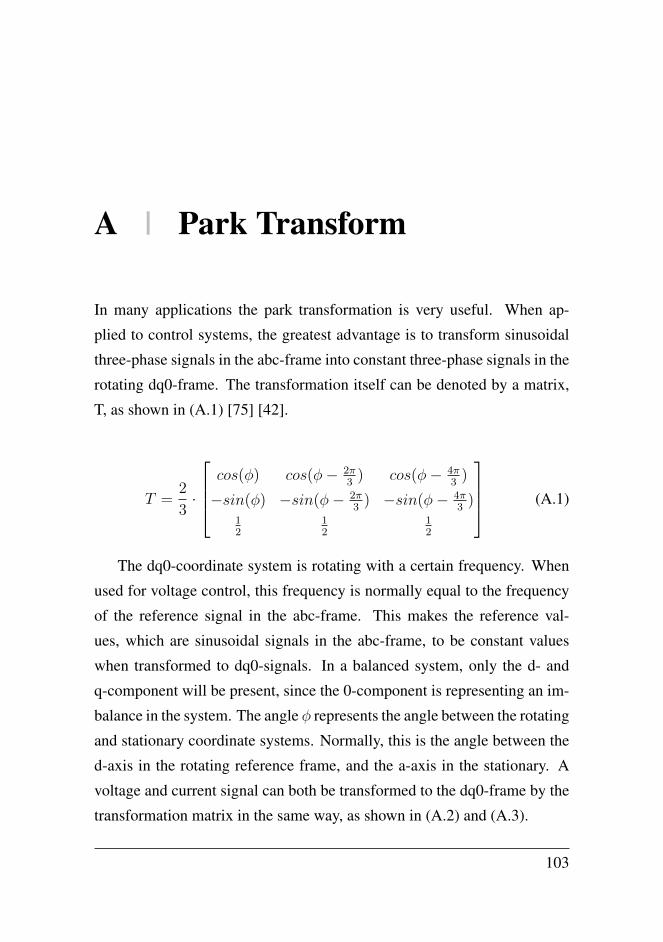
A | Park Transform
In many applications the park transformation is very useful. When ap-
plied to control systems, the greatest advantage is to transform sinusoidal
three-phase signals in the abc-frame into constant three-phase signals in the
rotating dq0-frame. The transformation itself can be denoted by a matrix,
T, as shown in (A.1) [75] [42].
T =2
3·
cos(φ) cos(φ− 2π
3) cos(φ− 4π
3)
−sin(φ) −sin(φ− 2π3
) −sin(φ− 4π3
)12
12
12
(A.1)
The dq0-coordinate system is rotating with a certain frequency. When
used for voltage control, this frequency is normally equal to the frequency
of the reference signal in the abc-frame. This makes the reference val-
ues, which are sinusoidal signals in the abc-frame, to be constant values
when transformed to dq0-signals. In a balanced system, only the d- and
q-component will be present, since the 0-component is representing an im-
balance in the system. The angle φ represents the angle between the rotating
and stationary coordinate systems. Normally, this is the angle between the
d-axis in the rotating reference frame, and the a-axis in the stationary. A
voltage and current signal can both be transformed to the dq0-frame by the
transformation matrix in the same way, as shown in (A.2) and (A.3).
103
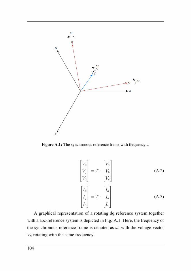
Figure A.1: The synchronous reference frame with frequency ω
Vd
Vq
V0
= T ·
Va
Vb
Vc
(A.2)
Id
Iq
I0
= T ·
Ia
Ib
Ic
(A.3)
A graphical representation of a rotating dq reference system together
with a abc-reference system is depicted in Fig. A.1. Here, the frequency of
the synchronous reference frame is denoted as ω, with the voltage vector
VS rotating with the same frequency.
104

B | Transfer Functions for Low-Pass Filters
In this appendix, the transfer functions for the L-, LC- and LCL-filters are
shown. The L-filters has a transfer function as shown in (B.1). Here, R
denotes the internal resistor in the inductor, L. ioutput denotes the output
current of the filter, and vinput the input voltage level.
GL =ioutputvinput
=1
sL+R(B.1)
The LC-filter has a transfer function as shown in (B.2). Here, the trans-
fer function is a relation between the input- and output voltage, instead
of the input voltage and output current, as for the L- and LCL-filter. A
comparison between the transfer functions’ bode-plot will however make it
possible to see the difference in e.g. reasonant peak, as was done in Sec-
tion 2.3. In (B.2), the notation is similar as for the L-filter. In addition to
the parameters introduced for (B.1), voutput is the output voltage across the
capacitor, while RC is the resistance related to the capacitor, C.
GLC =voutputvinput
=1 +RCCs
s2LC + sC(RC +R) + 1(B.2)
The transfer function of the LCL-filter is shown in (B.4), where (B.3)
defines the resonant frequency, ωr.
105

ωr =
√1
L1C+
1
L2C+
1
L1L2
(R1R2 +R1RC +R2RC) (B.3)
GLCL(s) = ioutput(s)
vinput(s)= sRCC+1
s3L1L2C+s2(L2C(R1+RC)+L1C(R2+RC))+L1L2Cω2rs)+R1+R2
(B.4)
L1 and L2 denote the inverter-side and grid-side inductor, respectively.
R1 andR2 are the resistances related to these inductors. ioutput is the current
flowing through the grid-side inductor.
106
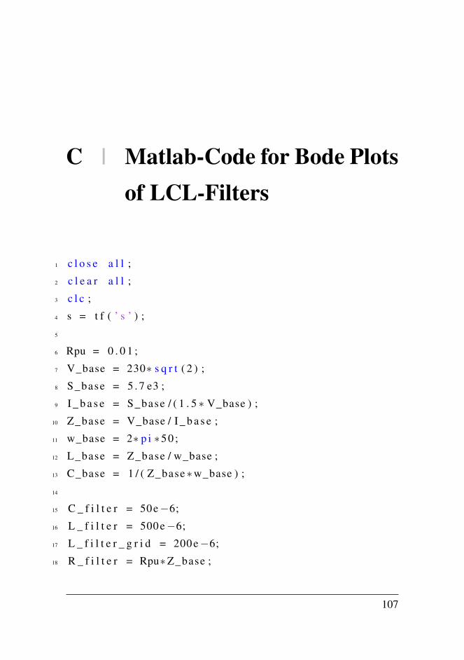
C | Matlab-Code for Bode Plotsof LCL-Filters
1 c l o s e a l l ;
2 c l e a r a l l ;
3 c l c ;
4 s = t f ( ’ s ’ ) ;
5
6 Rpu = 0 . 0 1 ;
7 V_base = 230∗ s q r t ( 2 ) ;
8 S_base = 5 . 7 e3 ;
9 I _ b a s e = S_base / ( 1 . 5 ∗ V_base ) ;
10 Z_base = V_base / I _ b a s e ;
11 w_base = 2∗ p i ∗50 ;
12 L_base = Z_base / w_base ;
13 C_base = 1 / ( Z_base ∗w_base ) ;
14
15 C _ f i l t e r = 50e−6;
16 L _ f i l t e r = 500 e−6;
17 L _ f i l t e r _ g r i d = 200 e−6;
18 R _ f i l t e r = Rpu∗Z_base ;
107
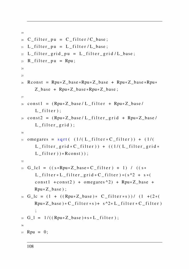
19
20 C _ f i l t e r _ p u = C _ f i l t e r / C_base ;
21 L _ f i l t e r _ p u = L _ f i l t e r / L_base ;
22 L _ f i l t e r _ g r i d _ p u = L _ f i l t e r _ g r i d / L_base ;
23 R _ f i l t e r _ p u = Rpu ;
24
25
26 Rcons t = Rpu∗Z_base ∗Rpu∗Z_base + Rpu∗Z_base ∗Rpu∗Z_base + Rpu∗Z_base ∗Rpu∗Z_base ;
27
28 c o n s t 1 = ( Rpu∗Z_base / L _ f i l t e r + Rpu∗Z_base /
L _ f i l t e r ) ;
29 c o n s t 2 = ( Rpu∗Z_base / L _ f i l t e r _ g r i d + Rpu∗Z_base /
L _ f i l t e r _ g r i d ) ;
30
31 omegares = s q r t ( ( 1 / ( L _ f i l t e r ∗ C _ f i l t e r ) ) + ( 1 / (
L _ f i l t e r _ g r i d ∗ C _ f i l t e r ) ) + ( ( 1 / ( L _ f i l t e r _ g r i d ∗L _ f i l t e r ) ) ∗Rcons t ) ) ;
32
33 G _ l c l = ( ( s ∗Rpu∗Z_base ∗ C _ f i l t e r ) + 1 ) / ( ( s ∗L _ f i l t e r ∗ L _ f i l t e r _ g r i d ∗ C _ f i l t e r ) ∗ ( s ^2 + s ∗ (
c o n s t 1 + c o n s t 2 ) + omegares ^2 ) + Rpu∗Z_base +
Rpu∗Z_base ) ;
34 G_lc = (1 + ( ( Rpu∗Z_base ) ∗ C _ f i l t e r ∗ s ) ) / (1 + ( 2∗ (
Rpu∗Z_base ) ∗ C _ f i l t e r ∗ s ) + s ^2∗ L _ f i l t e r ∗ C _ f i l t e r )
;
35 G_l = 1 / ( ( Rpu∗Z_base ) +s ∗ L _ f i l t e r ) ;
36
37 Rpu = 0 ;
108
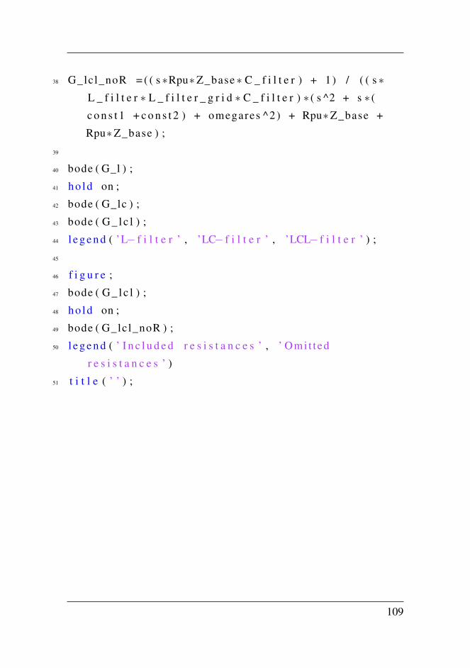
38 G_lcl_noR = ( ( s ∗Rpu∗Z_base ∗ C _ f i l t e r ) + 1 ) / ( ( s ∗L _ f i l t e r ∗ L _ f i l t e r _ g r i d ∗ C _ f i l t e r ) ∗ ( s ^2 + s ∗ (
c o n s t 1 + c o n s t 2 ) + omegares ^2 ) + Rpu∗Z_base +
Rpu∗Z_base ) ;
39
40 bode ( G_l ) ;
41 ho ld on ;
42 bode ( G_lc ) ;
43 bode ( G _ l c l ) ;
44 l e g e n d ( ’L− f i l t e r ’ , ’LC− f i l t e r ’ , ’LCL− f i l t e r ’ ) ;
45
46 f i g u r e ;
47 bode ( G _ l c l ) ;
48 ho ld on ;
49 bode ( G_lcl_noR ) ;
50 l e g e n d ( ’ I n c l u d e d r e s i s t a n c e s ’ , ’ Omi t ted
r e s i s t a n c e s ’ )
51 t i t l e ( ’ ’ ) ;
109

110
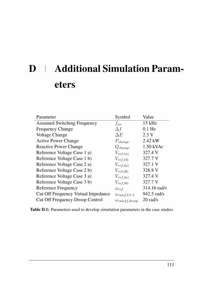
D | Additional Simulation Param-eters
Parameter Symbol ValueAssumed Switching Frequency fsw 15 kHzFrequency Change ∆f 0.1 HzVoltage Change ∆E 2.3 VActive Power Change Pchange 2.42 kWReactive Power Change Qchange 1.50 kVArReference Voltage Case 1 a) Vref,1a) 327.4 VReference Voltage Case 1 b) Vref,1b) 327.7 VReference Voltage Case 2 a) Vref,2a) 327.1 VReference Voltage Case 2 b) Vref,2b) 328.8 VReference Voltage Case 3 a) Vref,3a) 327.4 VReference Voltage Case 3 b) Vref,3b) 327.7 VReference Frequency ωref 314.16 rad/sCut Off Frequency Virtual Impedance ωcutoff,V.I. 942.5 rad/sCut Off Frequency Droop Control ωcutoff,droop 20 rad/s
Table D.1: Parameters used to develop simulation parameters in the case studies
111
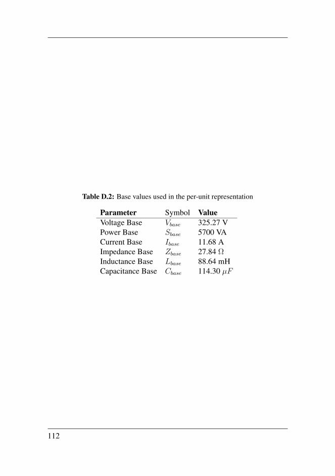
Table D.2: Base values used in the per-unit representation
Parameter Symbol ValueVoltage Base Vbase 325.27 VPower Base Sbase 5700 VACurrent Base Ibase 11.68 AImpedance Base Zbase 27.84 ΩInductance Base Lbase 88.64 mHCapacitance Base Cbase 114.30 µF
112
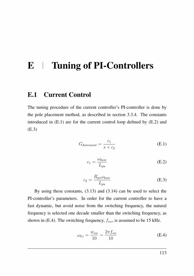
E | Tuning of PI-Controllers
E.1 Current Control
The tuning procedure of the current controller’s PI-controller is done by
the pole placement method, as described in section 3.3.4. The constants
introduced in (E.1) are for the current control loop defined by (E.2) and
(E.3)
Gdominant =c1
s+ c2(E.1)
c1 =ωbaseLpu
(E.2)
c2 =RpuωbaseLpu
(E.3)
By using these constants, (3.13) and (3.14) can be used to select the
PI-controller’s parameters. In order for the current controller to have a
fast dynamic, but avoid noise from the switching frequency, the natural
frequency is selected one decade smaller than the switching frequency, as
shown in (E.4). The switching frequency, fsw, is assumed to be 15 kHz.
ω0,i =wsw10
=2πfsw
10(E.4)
113

E.2 Voltage Control
Similarly as for the current controller, the voltage controller contains a PI-
controller tuned by the use of pole placement. The parameters used here
are decided on the basis of a natural frequency one decade lower than the
current controller’s natural frequency, as shown in (E.5). This to be sure
that the difference in bandwidth between the two controllers are sufficiently
large.
ω0,v =ω0,i
10=
2πfsw100
(E.5)
The constants in (E.1) are given by (E.6) and (E.7) for the voltage con-
troller.
c1 =ωbaseCpu
(E.6)
c2 = 0 (E.7)
These constant are then used in (3.13) and (3.14) to decide the PI-
controller’s proportional and integrator gain.
114
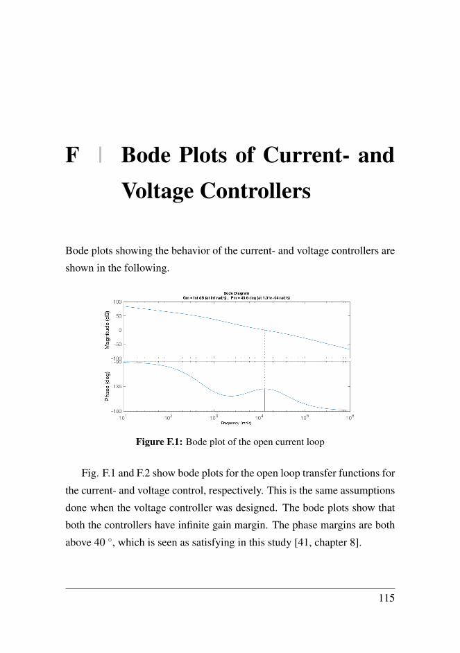
F | Bode Plots of Current- andVoltage Controllers
Bode plots showing the behavior of the current- and voltage controllers are
shown in the following.
Figure F.1: Bode plot of the open current loop
Fig. F.1 and F.2 show bode plots for the open loop transfer functions for
the current- and voltage control, respectively. This is the same assumptions
done when the voltage controller was designed. The bode plots show that
both the controllers have infinite gain margin. The phase margins are both
above 40 , which is seen as satisfying in this study [41, chapter 8].
115
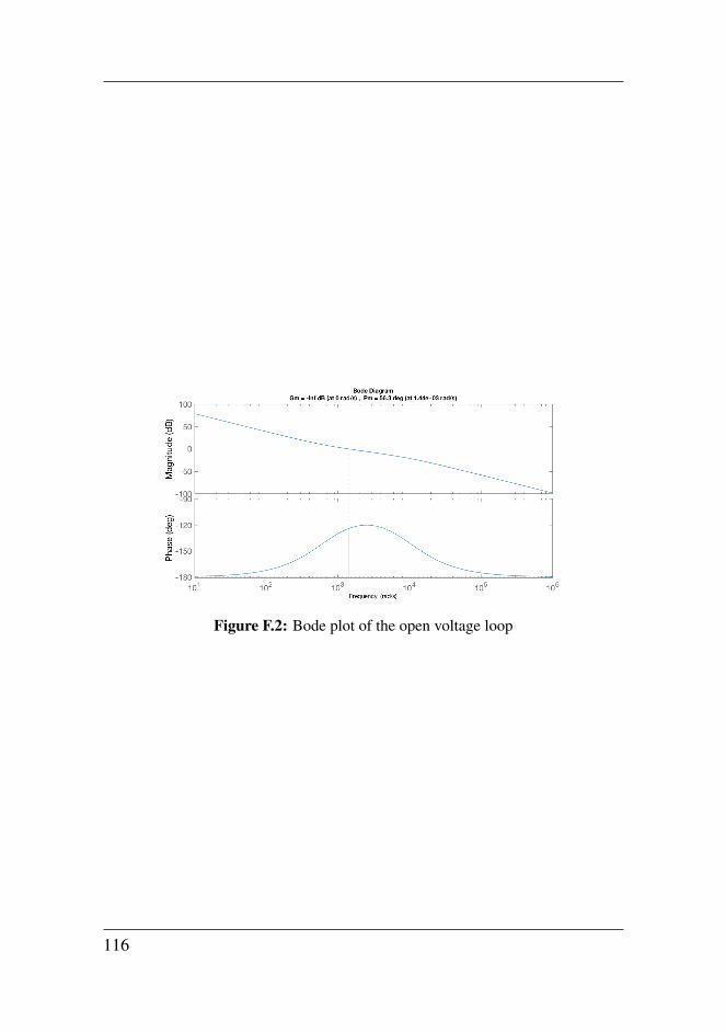
Figure F.2: Bode plot of the open voltage loop
116

G | MATLAB-Code for Bode-Plotsof Current- and Voltage Con-trollers
1 %Bode p l o t s
2 c l o s e a l l ;
3 c l e a r a l l ;
4 %%
5 Ts = 2e−5;
6 Tspwm = 2e−7;
7
8 w_ref = 2∗ p i ∗50 ;
9 E r e f = 400∗ s q r t ( 2 ) / s q r t ( 3 ) ;
10
11 d e l t a f = 0 . 1 ;
12 d e l t a o m e g a = d e l t a f ∗2∗ p i ;
13 Sload = 5 . 7 e3 ;
14 pf = 0 . 8 5 ;
15 Pload = Sload ∗ pf ;
16 Qload = s q r t ( S load ^2 − Pload ^2 ) ;
117
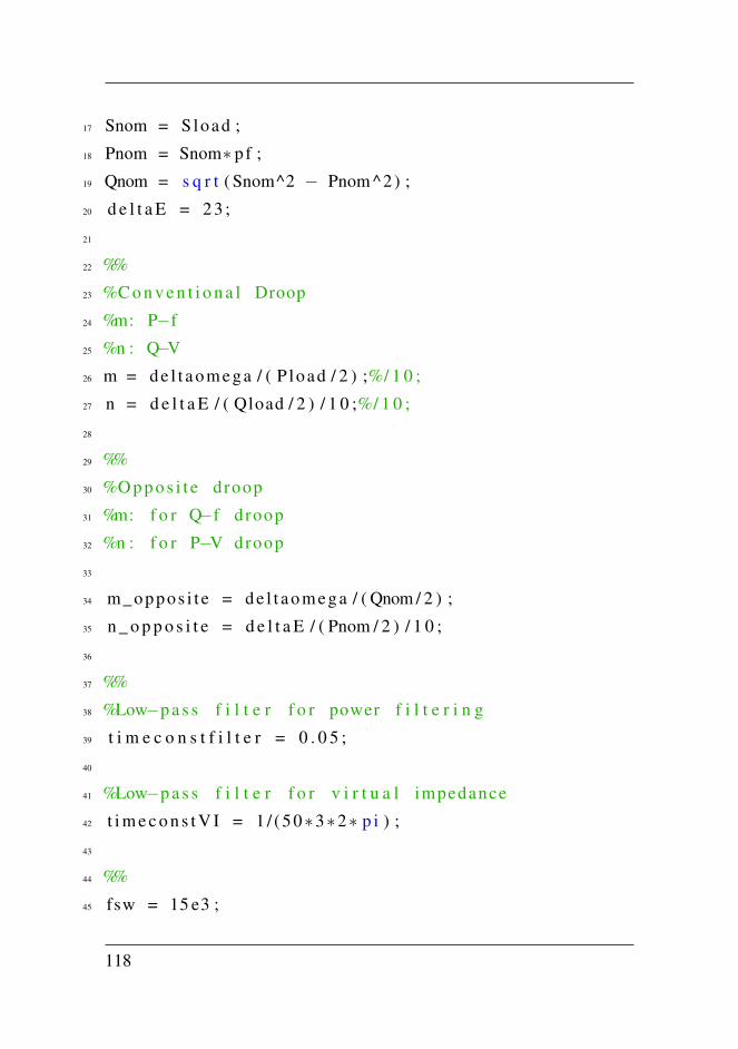
17 Snom = Sload ;
18 Pnom = Snom∗ pf ;
19 Qnom = s q r t ( Snom^2 − Pnom ^2) ;
20 d e l t a E = 2 3 ;
21
22 %%
23 %C o n v e n t i o n a l Droop
24 %m: P−f
25 %n : Q−V
26 m = d e l t a o m e g a / ( P load / 2 ) ;%/ 1 0 ;
27 n = d e l t a E / ( Qload / 2 ) / 1 0 ;%/ 1 0 ;
28
29 %%
30 %O p p o s i t e droop
31 %m: f o r Q−f droop
32 %n : f o r P−V droop
33
34 m_oppos i t e = d e l t a o m e g a / ( Qnom / 2 ) ;
35 n _ o p p o s i t e = d e l t a E / ( Pnom / 2 ) / 1 0 ;
36
37 %%
38 %Low−p a s s f i l t e r f o r power f i l t e r i n g
39 t i m e c o n s t f i l t e r = 0 . 0 5 ;
40
41 %Low−p a s s f i l t e r f o r v i r t u a l impedance
42 t i m e c o n s t V I = 1 / ( 5 0∗3∗2∗ p i ) ;
43
44 %%
45 fsw = 15 e3 ;
118
46 Rpu = 0 . 0 1 ;
47 rho = 0 . 7 ;
48 t _ d e l a y = 0 . 5 ∗ ( 1 / fsw ) ;
49 T_eq = 2∗ t _ d e l a y ;
50 wsw = 2∗ p i ∗ fsw ;
51
52 V_base = 230∗ s q r t ( 2 ) ;
53 S_base = Snom ;
54 I _ b a s e = S_base / ( 1 . 5 ∗ V_base ) ;
55 Z_base = V_base / I _ b a s e ;
56 w_base = 2∗ p i ∗50 ;
57 L_base = Z_base / w_base ;
58 C_base = 1 / ( Z_base ∗w_base ) ;
59
60 %%
61 %F i l t e r Va lues
62 C _ f i l t e r = 50e−6;
63 L _ f i l t e r = 500 e−6;
64 L _ f i l t e r _ g r i d = 200 e−6;
65 R _ f i l t e r _ p u = 0 . 0 1 ;
66 R _ f i l t e r = R _ f i l t e r _ p u ∗Z_base ;
67
68 C _ f i l t e r _ p u = C _ f i l t e r / C_base ;
69 L _ f i l t e r _ p u = L _ f i l t e r / L_base ;
70 L _ f i l t e r _ g r i d _ p u = L _ f i l t e r _ g r i d / L_base ;
71 R _ f i l t e r _ p u = R _ f i l t e r / Z_base ;
72 %%
73 %c u r r e n t c o n t r o l
74 w_oi = wsw / 1 0 ;
119
75 a = w_base∗Rpu / L _ f i l t e r _ p u ;
76 c = w_base / L _ f i l t e r _ p u ;
77 %
78 K_pi = ( ( 2∗ rho ∗w_oi )−a ) / c ;
79 K_i i = ( w_oi ) ^2 / c ;
80
81 %%
82 %V o l t a g e c o n t r o l
83 w_ov = w_oi / 1 0 ;
84
85 K_pv = (2∗ rho ∗w_ov∗ C _ f i l t e r _ p u ) / w_base ;
86 K_iv = ( w_ov∗w_ov∗ C _ f i l t e r _ p u ) / w_base ;
87 %%
88 fsw = 15 e3 ;
89 Lpu = L _ f i l t e r _ p u ;
90 Rpu = R _ f i l t e r _ p u ;
91 Cpu = C _ f i l t e r _ p u ;
92 wbase = 2∗ p i ∗50 ;
93 s = t f ( ’ s ’ ) ;
94 t _ d e l a y = 0 . 5 / fsw ;
95 rho = 0 . 7 ;
96 %%
97 %C u r r e n t c o n t r o l l e r
98 G p h y s i c a l i = ( 1 / Rpu ) / ( 1 + ( Lpu / ( Rpu∗wbase ) ∗ s ) ) ;
99 GPWMi = 1 / ( 1 + t _ d e l a y ∗ s ) ;
100 GPIi = K_pi + K_i i / s ;
101
102 Gol i = GPIi ∗GPWMi∗G p h y s i c a l i ;
103 G c l i = Go l i / (1+ Go l i ) ;
120

104 f i g u r e ( 1 ) ;
105 margin ( Go l i ) ;
106
107 %%
108 d e l a y c u r r e n t = 1 / w_oi ;
109 G d e l a y c u r r e n t = 1 / ( 1 + d e l a y c u r r e n t ∗ s ) ;
110 %V o l t a g e C o n t r o l l e r
111 G p h y s i c a l v = wbase / ( s ∗Cpu ) ;
112 GPIv = K_pv + K_iv / s ;
113 Golv = G p h y s i c a l v ∗GPIv∗G d e l a y c u r r e n t ;
114 Gclv = Golv / (1+ Golv ) ;
115
116 f i g u r e ( 2 ) ;
117 margin ( Golv ) ;
121

122

H | Response of the Controllers
In the following, the behavior of the current- and voltage controller will
be shown, in addition to both of the droop controllers. The simulations
for generating these plots are utilized in a microgrid system without use of
virtual impedance.
Figure H.1 and H.2 show how the conventional and the opposite droop
controllers follow their reference for one inverter. The figures also show
that the conventional droop controller have an accurate active power re-
sponse, while the reactive power is inaccurate. This causes the poor reactive
power sharing mentioned in Chapter 4. A similar behavior is shown for the
opposite droop control, but this controller provides accurate reactive power
dispatch, while there is a significant error in the active power. By Fig. H.1
and H.2, it can be seen that the control speed of the two droop controllers
provide a similar control speed, with a stable response after around 0.3 s.
The voltage controller’s response is shown in Fig. H.3. The control
speed is much faster than for the droop controllers. An accurate response is
provided, both for the d- and q-axis components, where there is a maximum
overshoot of around 0.2 pu. The voltage level is relatively stable after 0.1
s, so around three times faster than the outer power control provided by the
droop controllers.
The current controller’s response is shown in Fig. H.4. The current
reference in this figure is not constant, since the reference is given by the
123
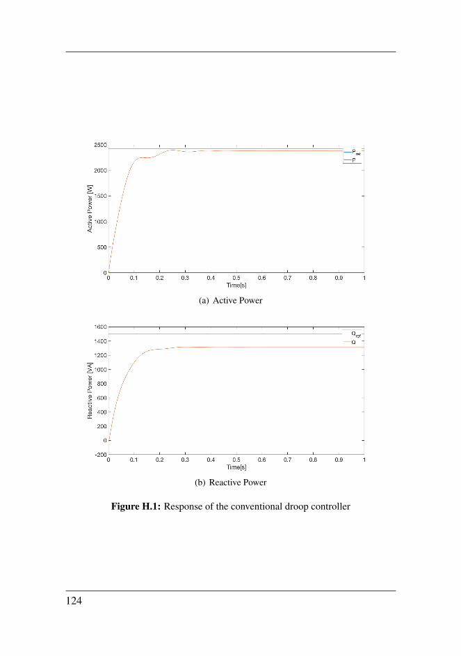
(a) Active Power
(b) Reactive Power
Figure H.1: Response of the conventional droop controller
124
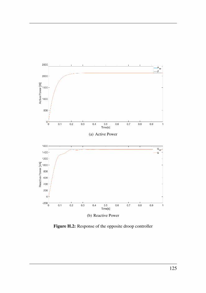
(a) Active Power
(b) Reactive Power
Figure H.2: Response of the opposite droop controller
125

(a) d-axis
(b) q-axis
Figure H.3: Response of the voltage controller
126

(a) d-axis
(b) q-axis
Figure H.4: Response of the current controller
127

slower voltage- and power control. The current control speed is much faster
than the two other controllers, where the output current follows the refer-
ence signal relatively close at around 1.5 ms. Since the parameters are
chosen so the controller should be 10 times faster than the voltage control,
this is seen as reasonable. With a not-constant current reference, the control
is more challenging, causing a slower response.
128
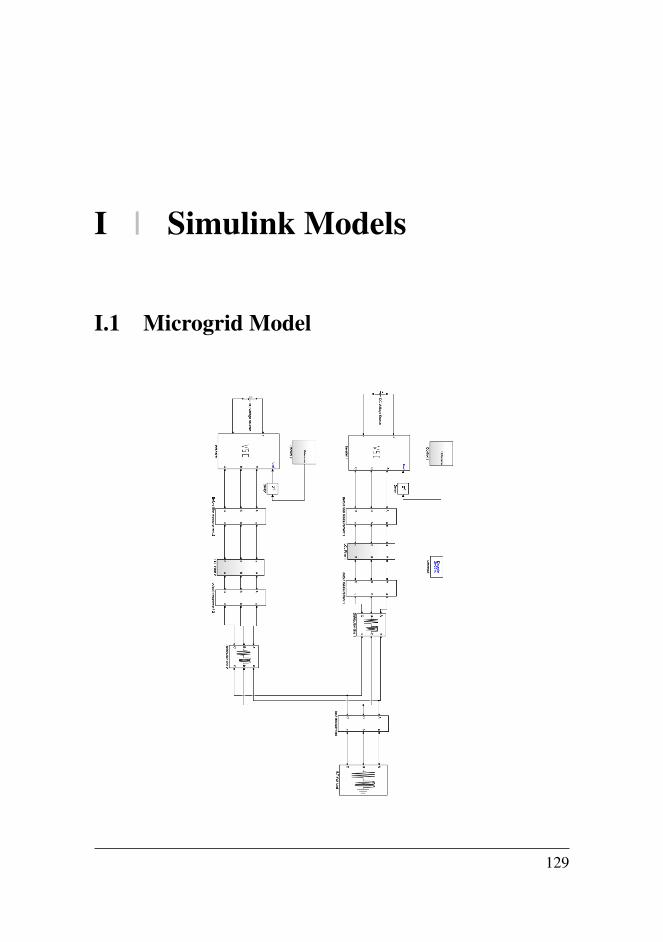
I | Simulink Models
I.1 Microgrid Model
129

I.2 Current Controller
130
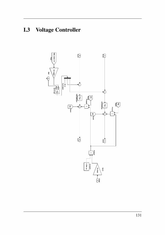
I.3 Voltage Controller
131
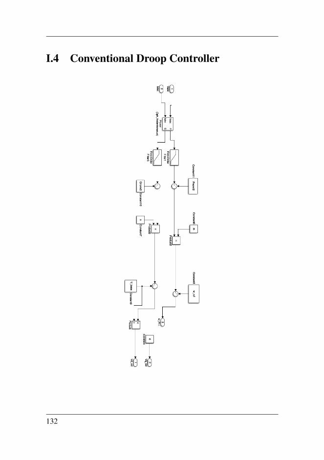
I.4 Conventional Droop Controller
132
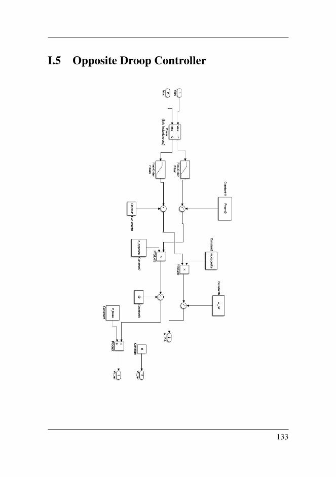
I.5 Opposite Droop Controller
133
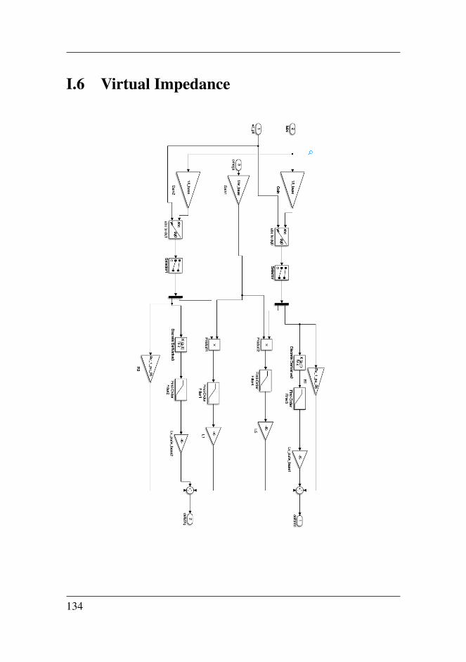
I.6 Virtual Impedance
134
J | Chapter 2 from "Control ofPower Electronics in Micro-grids"
135
2 | Literature Review
2.1 Microgrids
2.1.1 Definition
A microgrid is defined as a distribution system including distributed energy re-sources (DER), energy storage systems (ESS) and flexible loads [2, chapter 1].It has clearly defined electrical boundaries, and from the main grid, the microgridshould be controllable as a single unit. It has two main operation modes. These arethe grid connected mode and "island mode", where the microgrid is disconnectedfrom the main grid. This capability is a strong feature, and advantageous when itcomes to securing the electricity supply in the grid [9].
2.1.2 Fundamental components
In the operation of a microgrid, there are a number of essential controllable com-ponents. With a large amount of unreliable distributed generation, the voltage andpower levels from this generation and the energy storage need to be controlled.When operating in grid-connected mode, there has to be a proper interaction withthe main grid [14].
A lot of the distributed generation, e.g. a PV-system and also a battery storagedevice, are based on DC [15, chapter 6]. When connected to a DC-microgrid, aDC/DC-converter is used to convert the voltage level, while in a AC-microgrid, anDC/AC-inverter is used to convert the voltage to a proper AC-voltage [16, chap-ter 8].
In the following sections, some of the main components of a microgrid will beintroduced.
Distributed Generation
One of the things that characterize a microgrid, is the use of distributed generation[9] [2, chapter 1]. In contrast to large generation units in the traditional power

Chapter 2. Literature Review
Figure 2.1: A schematic showing a voltage source converter
grid, the DGs are normally much smaller, also in terms of power [17]. A lot ofthe DGs are based on renewable energy resources, which makes them particularlyimportant because of their importance in the future power grid [7].
DG, such as PV-systems and wind-turbines, are clearly dependent on the weather.With less reliable generation, the need for ESSs increases for the required powerto be supplied [18]. In contrast to traditional rotating generators, many of the DGsdo not have any rotating mass [19]. This leads to challenges when it comes tofrequency regulation, as will be further discussed in section 2.2. In section 2.1.7,challenges related to the interaction between several DGs will be studied.
Voltage Source Converter
Many of the technologies used for DG are based on DC-voltage [15, chapter 6] [15,chapter 8]. In the process of converting a DC-voltage to a three-phase AC-voltage,or opposite, a three-phase voltage source converter (VSC) can be used [17]. Aschematic is shown in Fig. 2.1. When the power flow is from the DC to the ACside, the converter operates as an inverter. The output of a three-phase voltagesource inverter (VSI) is decided by the input DC-voltage and the operating of thesemiconducting devices, acting as switches. A frequently used method to createcontrol signals for VSCs is the pulse width modulation method [16, chapter 8]. Acomparison between the reference output waveform and a high-frequency trian-gular waveform is then used to generate a control signal for the semiconductingdevices.
When the power flow can be bidirectional, for example in case of a battery, theVSC has to be able to operate both as an inverter and a rectifier [16]. In this work,the operation of the VSCs are limited to inverter operation.
2.1 Microgrids
Energy Storage System
The ESS can store surplus energy from DGs, and at times with lower generation,it can assist the DGs and the main grid with the power supply [15, chapter 9]. Bybalancing the difference between production and load, it also helps stabilizing thevoltage and frequency in a microgrid, especially in island mode operation [20].The total storage capacity of a microgrid can consist of one large ESS, or severalsmaller units, where the total capacity of the microgrid can contribute to decidehow long the it can operate in island mode [15, chapter 9]. Electrical vehicles’s(EV’s) battery can also contribute to the energy storage capacity of the microgrid,through a vehicle-to-grid-solution [21] [11]. For the ESSs, several technologies areavailable. Examples of common alternatives are flywheel energy storage (FES),supercapacitors and batteries, which will briefly introduced in the following.
In a flywheel energy storage, kinetic energy are stored in a rotating system.By using an electric machine, the flywheel is accelerated, while the flywheel isdecelerated when electricity is generated from it. Normally, FESs are used forrelatively short time energy storage.[22][23].
A supercapacitor is a large capacitor where the energy is stored as static charge.They are also best suited for applications where short-term charging is needed.Both supercapacitors and FES systems have long lifetime, including many cyclingtimes without much maintenance [23].
Battery Energy Storage (BES) systems are probably the most used energy stor-age alternative among these, and one of the most used technologies on the market[23]. The energy is stored as electrochemical energy, with several technologiesavailable. Many of these technologies can be used for long term storage, but thecapability for number of cycling times can be a drawback compared to the otheralternatives [22].
Loads
The loads connected to a microgrid will have great influence on the electrical pa-rameters, such as current and voltage levels. With more power electronics, theamount of non-linear loads in the power grid will increase [16, chapter 5]. Theseload also make strict demands on the microgrids control system, in order to keepthe electrical parameters within required boundaries [2, chapter 2].
Also, the number of controllable loads can be increased. An example is theelectrical vehicles, as already mentioned. They can operate not only as loads, butalso as a part of the storage capacity of the grid. Then, a control system must beconnected to ensure the charging, as well as controlling the possible reverse powerflow.
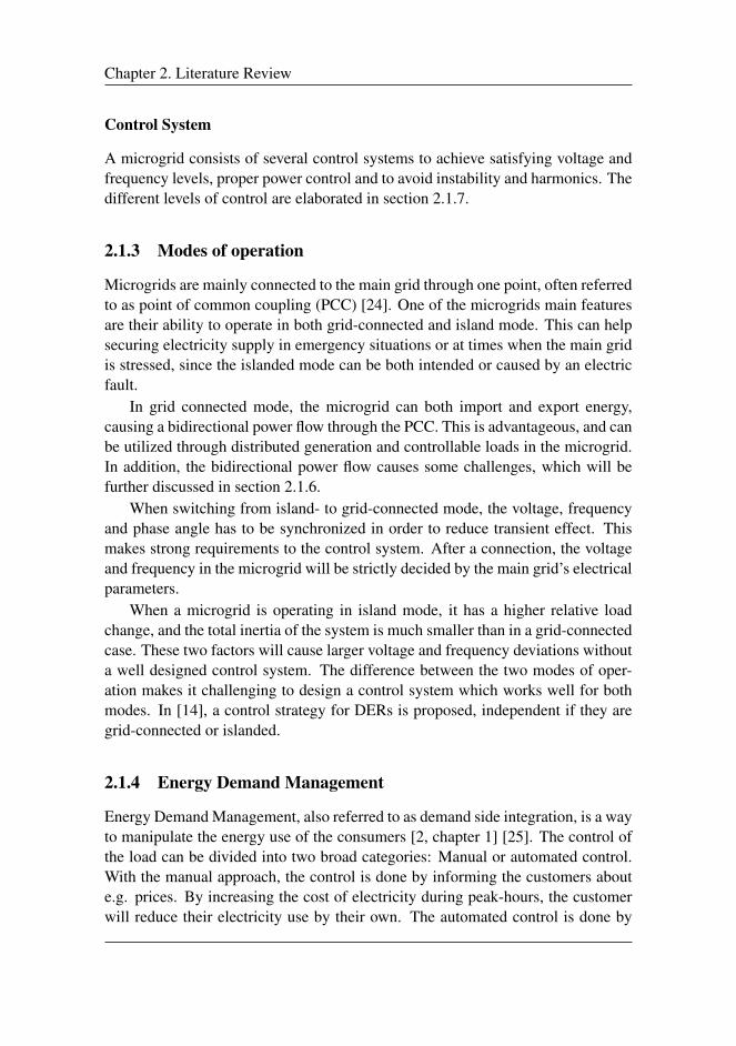
Chapter 2. Literature Review
Control System
A microgrid consists of several control systems to achieve satisfying voltage andfrequency levels, proper power control and to avoid instability and harmonics. Thedifferent levels of control are elaborated in section 2.1.7.
2.1.3 Modes of operation
Microgrids are mainly connected to the main grid through one point, often referredto as point of common coupling (PCC) [24]. One of the microgrids main featuresare their ability to operate in both grid-connected and island mode. This can helpsecuring electricity supply in emergency situations or at times when the main gridis stressed, since the islanded mode can be both intended or caused by an electricfault.
In grid connected mode, the microgrid can both import and export energy,causing a bidirectional power flow through the PCC. This is advantageous, and canbe utilized through distributed generation and controllable loads in the microgrid.In addition, the bidirectional power flow causes some challenges, which will befurther discussed in section 2.1.6.
When switching from island- to grid-connected mode, the voltage, frequencyand phase angle has to be synchronized in order to reduce transient effect. Thismakes strong requirements to the control system. After a connection, the voltageand frequency in the microgrid will be strictly decided by the main grid’s electricalparameters.
When a microgrid is operating in island mode, it has a higher relative loadchange, and the total inertia of the system is much smaller than in a grid-connectedcase. These two factors will cause larger voltage and frequency deviations withouta well designed control system. The difference between the two modes of oper-ation makes it challenging to design a control system which works well for bothmodes. In [14], a control strategy for DERs is proposed, independent if they aregrid-connected or islanded.
2.1.4 Energy Demand Management
Energy Demand Management, also referred to as demand side integration, is a wayto manipulate the energy use of the consumers [2, chapter 1] [25]. The control ofthe load can be divided into two broad categories: Manual or automated control.With the manual approach, the control is done by informing the customers aboute.g. prices. By increasing the cost of electricity during peak-hours, the customerwill reduce their electricity use by their own. The automated control is done by

2.1 Microgrids
shifting loads automatically, where the shifting is based on predefined considera-tions.
In the automated energy demand management, energy storage devices playan important role. During peak-hours, a larger amount of power can be suppliedfrom the batteries, to reduce the main grid’s stress. This is done by a conceptoften referred to as "peak shaving and valley filling" [15, chapter 9]. The ESS ischarged when the load is low, to supply energy at higher-load hours, where thedeviation between the DERs production and the total load of the system is thelargest. Controllable, flexible loads can also contribute to a good energy demandmanagement, for instance by specifying when an EV should be fully charged. Aslong as this is met, the battery of the EV can contribute to the grid, as described inpreviously.
2.1.5 Ancillary Services
Since microgrids behave as a single unit from the main grid, they have the ability toprovide several ancillary services. They can offer services such as energy demandmanagement, supply of reactive power and contribution to voltage and frequencyregulation. These features are powerful attributes of microgrids, where many ofthem are dependent of the ESS.
2.1.6 Technical Challenges
The operation of a microgrid has several technical challenges, compared to theoperation of the large power grid. Some of the main challenges can be classifiedas follows [17].
1. Stability and Power Quality: Many generation units, loads and control sys-tems can cause disturbances. This can affect both the power quality andstability.
2. Protection: More DG also leads to power flow issues such as circulatingcurrents and problems connected to bidirectional power flows. The protec-tion challenges increases, including voltage and frequency control and faultcurrents for instance.
3. Low Moment of Inertia: With more inverter-based generation, the amount ofrotating mass in the system will decrease. This can lead to large frequencydeviations, especially when operting in island mode.
4. Uncertainty: More DG based on RES can cause larger reliability issues,since many of the generation units will be non-controllable.
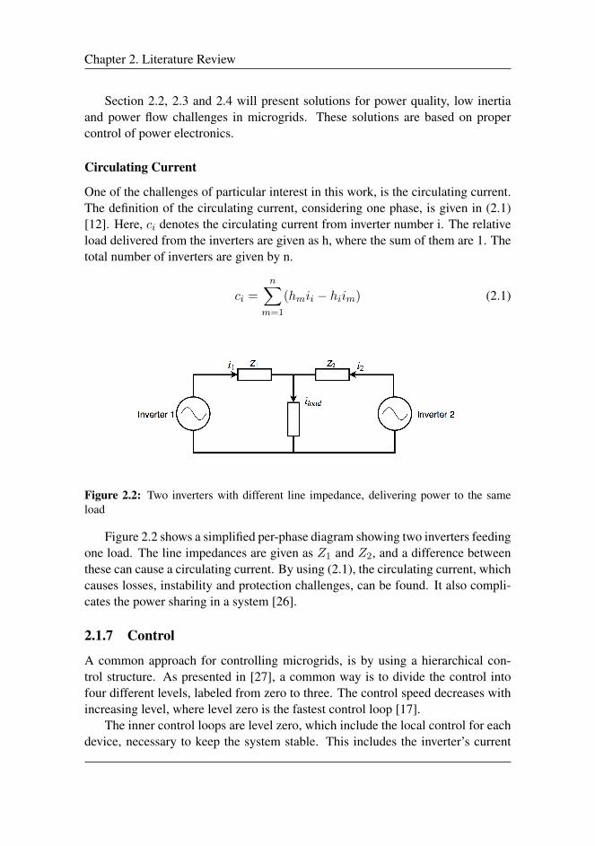
Chapter 2. Literature Review
Section 2.2, 2.3 and 2.4 will present solutions for power quality, low inertiaand power flow challenges in microgrids. These solutions are based on propercontrol of power electronics.
Circulating Current
One of the challenges of particular interest in this work, is the circulating current.The definition of the circulating current, considering one phase, is given in (2.1)[12]. Here, ci denotes the circulating current from inverter number i. The relativeload delivered from the inverters are given as h, where the sum of them are 1. Thetotal number of inverters are given by n.
ci =
nX
m=1
(hmii hiim) (2.1)
Figure 2.2: Two inverters with different line impedance, delivering power to the sameload
Figure 2.2 shows a simplified per-phase diagram showing two inverters feedingone load. The line impedances are given as Z1 and Z2, and a difference betweenthese can cause a circulating current. By using (2.1), the circulating current, whichcauses losses, instability and protection challenges, can be found. It also compli-cates the power sharing in a system [26].
2.1.7 Control
A common approach for controlling microgrids, is by using a hierarchical con-trol structure. As presented in [27], a common way is to divide the control intofour different levels, labeled from zero to three. The control speed decreases withincreasing level, where level zero is the fastest control loop [17].
The inner control loops are level zero, which include the local control for eachdevice, necessary to keep the system stable. This includes the inverter’s current
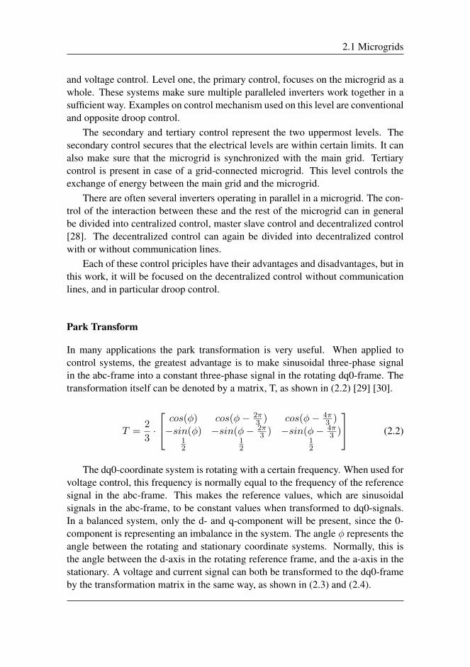
2.1 Microgrids
and voltage control. Level one, the primary control, focuses on the microgrid as awhole. These systems make sure multiple paralleled inverters work together in asufficient way. Examples on control mechanism used on this level are conventionaland opposite droop control.
The secondary and tertiary control represent the two uppermost levels. Thesecondary control secures that the electrical levels are within certain limits. It canalso make sure that the microgrid is synchronized with the main grid. Tertiarycontrol is present in case of a grid-connected microgrid. This level controls theexchange of energy between the main grid and the microgrid.
There are often several inverters operating in parallel in a microgrid. The con-trol of the interaction between these and the rest of the microgrid can in generalbe divided into centralized control, master slave control and decentralized control[28]. The decentralized control can again be divided into decentralized controlwith or without communication lines.
Each of these control priciples have their advantages and disadvantages, but inthis work, it will be focused on the decentralized control without communicationlines, and in particular droop control.
Park Transform
In many applications the park transformation is very useful. When applied tocontrol systems, the greatest advantage is to make sinusoidal three-phase signalin the abc-frame into a constant three-phase signal in the rotating dq0-frame. Thetransformation itself can be denoted by a matrix, T, as shown in (2.2) [29] [30].
T =2
3·
24
cos() cos( 23 ) cos( 4
3 )sin() sin( 2
3 ) sin( 43 )
12
12
12
35 (2.2)
The dq0-coordinate system is rotating with a certain frequency. When used forvoltage control, this frequency is normally equal to the frequency of the referencesignal in the abc-frame. This makes the reference values, which are sinusoidalsignals in the abc-frame, to be constant values when transformed to dq0-signals.In a balanced system, only the d- and q-component will be present, since the 0-component is representing an imbalance in the system. The angle represents theangle between the rotating and stationary coordinate systems. Normally, this isthe angle between the d-axis in the rotating reference frame, and the a-axis in thestationary. A voltage and current signal can both be transformed to the dq0-frameby the transformation matrix in the same way, as shown in (2.3) and (2.4).

Chapter 2. Literature Review
Figure 2.3: A representation of power flow through a line
24
Vd
Vq
V0
35 = T ·
24
Va
Vb
Vc
35 (2.3)
24
Id
Iq
I0
35 = T ·
24
Ia
Ib
Ic
35 (2.4)
Droop Control
Droop control is a distributed control algorithm where the power flow is controlledwithout need for communication between the inverters [6, chapter 9] [28]. Theprinciple is based on the relation between the active and reactive power flow, andthe frequency and voltage in the grid.
By studying the power flow through a line, as shown in Fig. 2.3, the droopcontrol principle can be explained. With a line impedance represented by Z, theactive and reactive power flow in the line is given by (2.5) and (2.6) [28] [31].Here, represents the power angle, while is the angle of the impedance, Z. If asmall is assumed, sin() ' and cos() ' 1. By using these simplifications, can be expressed by (2.7), and the voltage drop by (2.8) [28] [32].
P =U2
1
Zcos() U1U2
Zcos( + ) (2.5)
Q =U2
1
Zsin() U1U2
Zsin( + ) (2.6)
' XP
U1U2(2.7)

2.1 Microgrids
U1 U2 ' XQ
U1(2.8)
By (2.7) and (2.8), the conventional droop characteristic is found, representedby (2.9) and (2.10) [17]. Here, mP and nQ are the active and reactive droopcoefficients. They decide the relation between frequency and active power, andvoltage and reactive power, respectively. Eref and !ref are the rated voltage andfrequency, while Pref and Qref are the set points for the active and reactive power[28]. E, !, P and Q are the measured values of the voltage, frequency and activeand reactive power. The conventional droop characteristic is summarized in Fig.2.4 [17].
In a pure reactive line the power angle, , is dependent on the active power,while the voltage drop on the reactive power. Therefore, the power angle can becontrolled by the active power fed into the line. Because of the relation between thepower angle and frequency [33, chapter 4.3.3], the active power fed into the linecan be controlled by the frequency deviations. The reactive power is controlled byvoltage fluctuations. This is the conventional droop control method[34] [28].
The droop coefficients mP and nP represent the change in frequency and volt-age amplitude relative to power. In the equations used in this work, the values ofm and n are always positive, they denote the absolute value of the slope in Fig.2.4 and 2.5. The transient responses in the microgrid can be controlled by thesecoefficients. In section 2.2, it is studied how the inverters behaviour can imitate thebehaviour of a synchronous machine when using the conventional droop control.These coefficients can also be customized to make different DGs feed the loaddifferently [34].
! !ref = mP (Pref P ) (2.9)
E Eref = nQ(Qref Q) (2.10)
In a purely resistive line, a similar correlation can be found. By (2.5) and (2.6),and still assuming that is small, (2.11) and (2.12) can be derived.
' RQ
U1U2(2.11)
U1 U2 ' RP
U1(2.12)
As it can be seen from these equations, the power angle, and therefore fre-quency, is now dependent on the reactive power, while the voltage drop depends
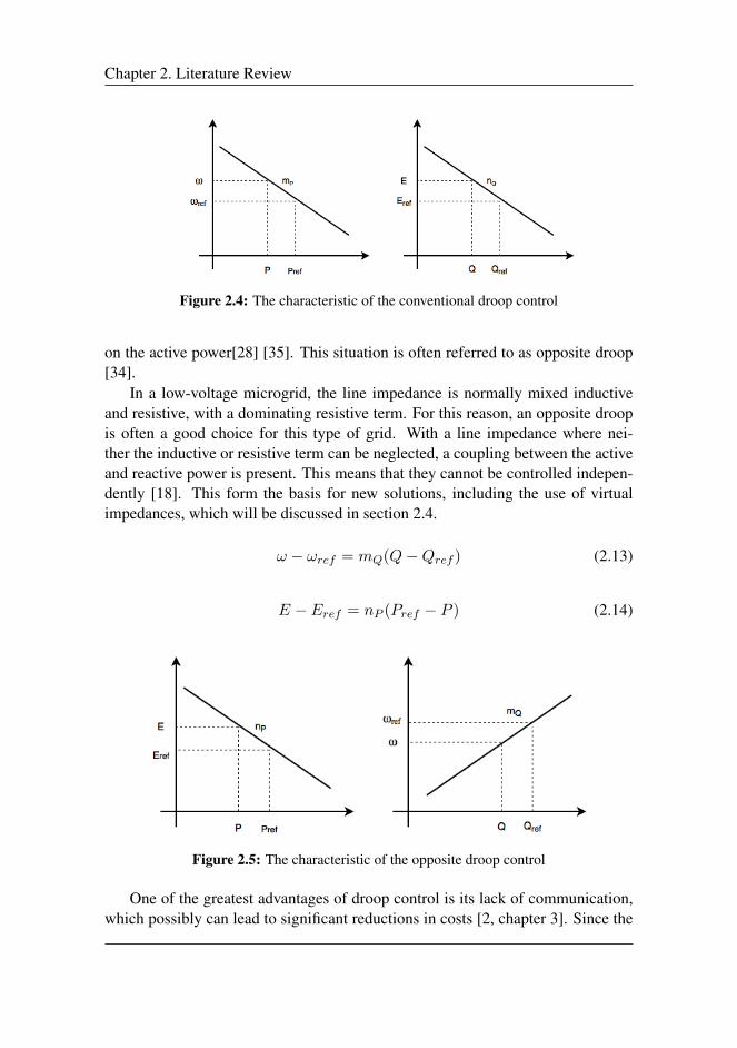
Chapter 2. Literature Review
Figure 2.4: The characteristic of the conventional droop control
on the active power[28] [35]. This situation is often referred to as opposite droop[34].
In a low-voltage microgrid, the line impedance is normally mixed inductiveand resistive, with a dominating resistive term. For this reason, an opposite droopis often a good choice for this type of grid. With a line impedance where nei-ther the inductive or resistive term can be neglected, a coupling between the activeand reactive power is present. This means that they cannot be controlled indepen-dently [18]. This form the basis for new solutions, including the use of virtualimpedances, which will be discussed in section 2.4.
! !ref = mQ(Q Qref ) (2.13)
E Eref = nP (Pref P ) (2.14)
Figure 2.5: The characteristic of the opposite droop control
One of the greatest advantages of droop control is its lack of communication,which possibly can lead to significant reductions in costs [2, chapter 3]. Since the
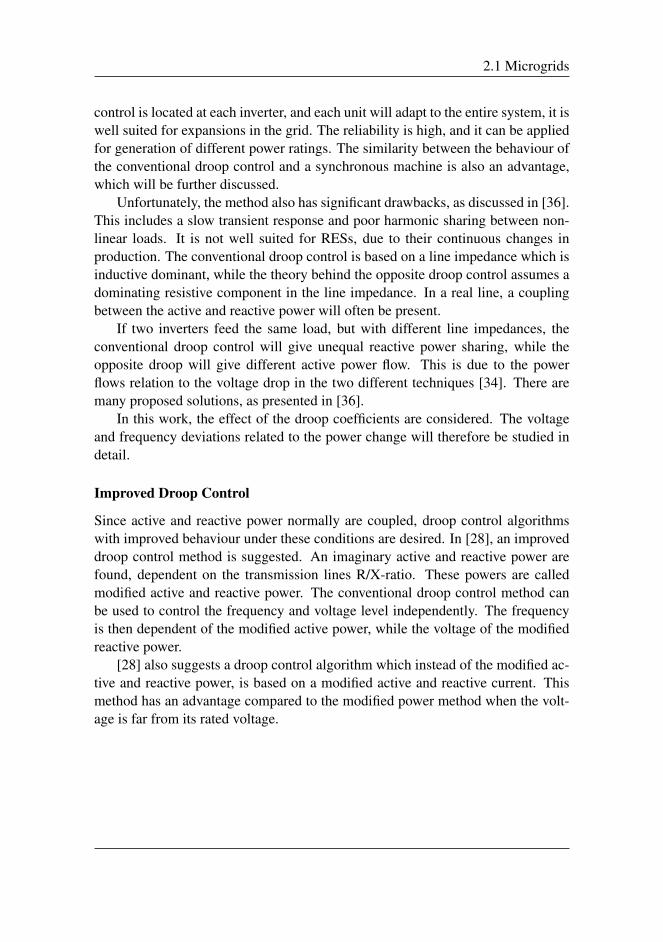
2.1 Microgrids
control is located at each inverter, and each unit will adapt to the entire system, it iswell suited for expansions in the grid. The reliability is high, and it can be appliedfor generation of different power ratings. The similarity between the behaviour ofthe conventional droop control and a synchronous machine is also an advantage,which will be further discussed.
Unfortunately, the method also has significant drawbacks, as discussed in [36].This includes a slow transient response and poor harmonic sharing between non-linear loads. It is not well suited for RESs, due to their continuous changes inproduction. The conventional droop control is based on a line impedance which isinductive dominant, while the theory behind the opposite droop control assumes adominating resistive component in the line impedance. In a real line, a couplingbetween the active and reactive power will often be present.
If two inverters feed the same load, but with different line impedances, theconventional droop control will give unequal reactive power sharing, while theopposite droop will give different active power flow. This is due to the powerflows relation to the voltage drop in the two different techniques [34]. There aremany proposed solutions, as presented in [36].
In this work, the effect of the droop coefficients are considered. The voltageand frequency deviations related to the power change will therefore be studied indetail.
Improved Droop Control
Since active and reactive power normally are coupled, droop control algorithmswith improved behaviour under these conditions are desired. In [28], an improveddroop control method is suggested. An imaginary active and reactive power arefound, dependent on the transmission lines R/X-ratio. These powers are calledmodified active and reactive power. The conventional droop control method canbe used to control the frequency and voltage level independently. The frequencyis then dependent of the modified active power, while the voltage of the modifiedreactive power.
[28] also suggests a droop control algorithm which instead of the modified ac-tive and reactive power, is based on a modified active and reactive current. Thismethod has an advantage compared to the modified power method when the volt-age is far from its rated voltage.
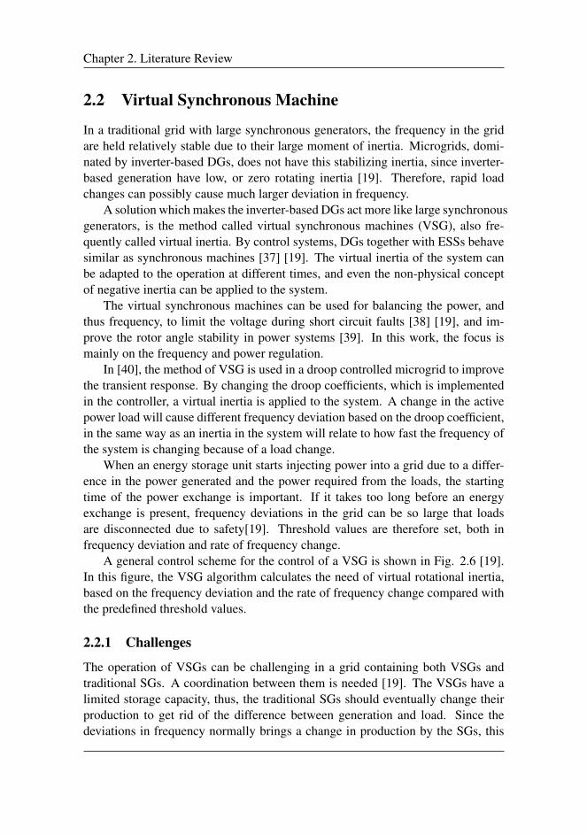
Chapter 2. Literature Review
2.2 Virtual Synchronous Machine
In a traditional grid with large synchronous generators, the frequency in the gridare held relatively stable due to their large moment of inertia. Microgrids, domi-nated by inverter-based DGs, does not have this stabilizing inertia, since inverter-based generation have low, or zero rotating inertia [19]. Therefore, rapid loadchanges can possibly cause much larger deviation in frequency.
A solution which makes the inverter-based DGs act more like large synchronousgenerators, is the method called virtual synchronous machines (VSG), also fre-quently called virtual inertia. By control systems, DGs together with ESSs behavesimilar as synchronous machines [37] [19]. The virtual inertia of the system canbe adapted to the operation at different times, and even the non-physical conceptof negative inertia can be applied to the system.
The virtual synchronous machines can be used for balancing the power, andthus frequency, to limit the voltage during short circuit faults [38] [19], and im-prove the rotor angle stability in power systems [39]. In this work, the focus ismainly on the frequency and power regulation.
In [40], the method of VSG is used in a droop controlled microgrid to improvethe transient response. By changing the droop coefficients, which is implementedin the controller, a virtual inertia is applied to the system. A change in the activepower load will cause different frequency deviation based on the droop coefficient,in the same way as an inertia in the system will relate to how fast the frequency ofthe system is changing because of a load change.
When an energy storage unit starts injecting power into a grid due to a differ-ence in the power generated and the power required from the loads, the startingtime of the power exchange is important. If it takes too long before an energyexchange is present, frequency deviations in the grid can be so large that loadsare disconnected due to safety[19]. Threshold values are therefore set, both infrequency deviation and rate of frequency change.
A general control scheme for the control of a VSG is shown in Fig. 2.6 [19].In this figure, the VSG algorithm calculates the need of virtual rotational inertia,based on the frequency deviation and the rate of frequency change compared withthe predefined threshold values.
2.2.1 Challenges
The operation of VSGs can be challenging in a grid containing both VSGs andtraditional SGs. A coordination between them is needed [19]. The VSGs have alimited storage capacity, thus, the traditional SGs should eventually change theirproduction to get rid of the difference between generation and load. Since thedeviations in frequency normally brings a change in production by the SGs, this
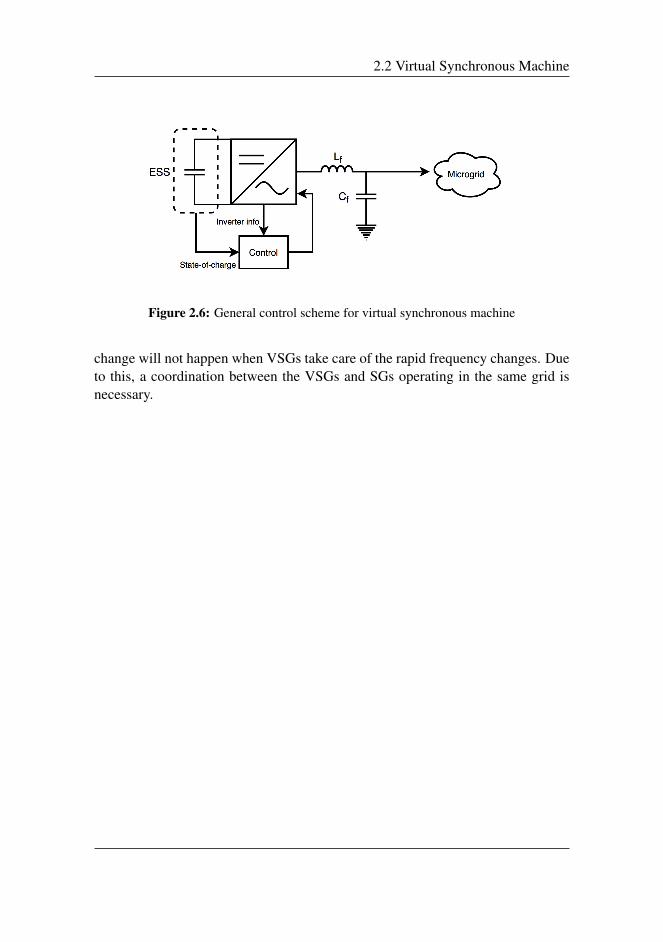
2.2 Virtual Synchronous Machine
Figure 2.6: General control scheme for virtual synchronous machine
change will not happen when VSGs take care of the rapid frequency changes. Dueto this, a coordination between the VSGs and SGs operating in the same grid isnecessary.

Chapter 2. Literature Review
2.3 Active Filtering
Power electronics devices provide several efficient services to the future electric-ity grid, but they also contribute to more non-linear loads in the system. Theseloads lead to harmonic and reactive currents [41]. Passive filters can be used forfiltering harmonics, but have drawbacks such as large size, resonance and fixedcompensation. Instead of these, power electronic devices can be used to compen-sate for harmonics. Such devices used to increase the power quality is known asactive filters (AFs), where for instance voltage source converters can be used. Thistechnique gives an improved filtering, but at a higher cost than passive filters.
To improve the power quality, AFs can provide voltage regulation, filteringharmonics, reactive power control and power factor correction[42] [43]. AFs canbe implemented both as series active filters, shunt active filters, as shown in Fig.2.8 and 2.7. An AF can also be a combination of the two, often called a powerquality conditioner [44].
The shunt AF is the most used of the active filtering techniques. Harmoniccurrents are fed by the filter to compensate for the harmonic currents flowing inthe line. An advantage of this technique is that the AF only has to be designed fora relatively small current, the harmonic compensating current. Figure 2.7 shows abasic illustration of the shunt AF in a grid.
Figure 2.7: A basic diagram showing a shunt active filter
Instead of current harmonics, series AFs cancel voltage harmonics. As shownin Fig. 2.8, it can be done by using a transformer, connected in series with the line.A drawback of this method is that the series AF has to carry the entire load current.The current ratings of these filters must therefore be much larger than for the shunt
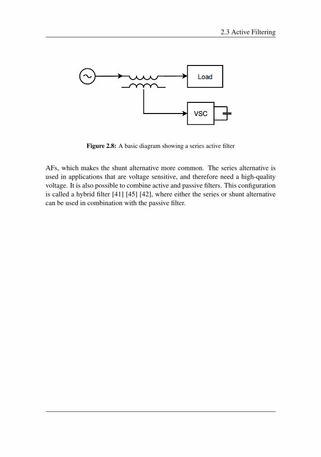
2.3 Active Filtering
Figure 2.8: A basic diagram showing a series active filter
AFs, which makes the shunt alternative more common. The series alternative isused in applications that are voltage sensitive, and therefore need a high-qualityvoltage. It is also possible to combine active and passive filters. This configurationis called a hybrid filter [41] [45] [42], where either the series or shunt alternativecan be used in combination with the passive filter.
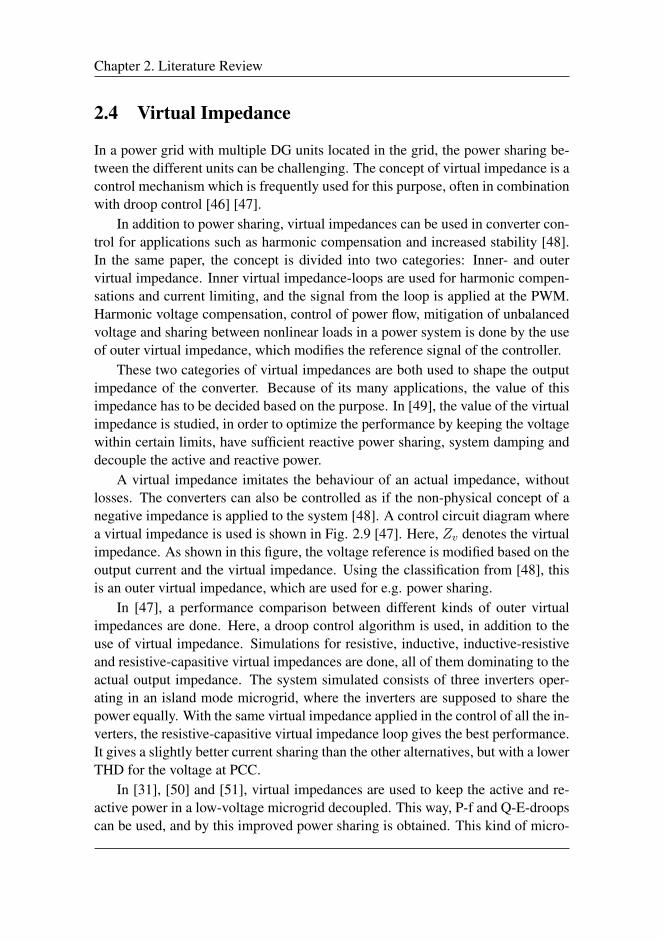
Chapter 2. Literature Review
2.4 Virtual Impedance
In a power grid with multiple DG units located in the grid, the power sharing be-tween the different units can be challenging. The concept of virtual impedance is acontrol mechanism which is frequently used for this purpose, often in combinationwith droop control [46] [47].
In addition to power sharing, virtual impedances can be used in converter con-trol for applications such as harmonic compensation and increased stability [48].In the same paper, the concept is divided into two categories: Inner- and outervirtual impedance. Inner virtual impedance-loops are used for harmonic compen-sations and current limiting, and the signal from the loop is applied at the PWM.Harmonic voltage compensation, control of power flow, mitigation of unbalancedvoltage and sharing between nonlinear loads in a power system is done by the useof outer virtual impedance, which modifies the reference signal of the controller.
These two categories of virtual impedances are both used to shape the outputimpedance of the converter. Because of its many applications, the value of thisimpedance has to be decided based on the purpose. In [49], the value of the virtualimpedance is studied, in order to optimize the performance by keeping the voltagewithin certain limits, have sufficient reactive power sharing, system damping anddecouple the active and reactive power.
A virtual impedance imitates the behaviour of an actual impedance, withoutlosses. The converters can also be controlled as if the non-physical concept of anegative impedance is applied to the system [48]. A control circuit diagram wherea virtual impedance is used is shown in Fig. 2.9 [47]. Here, Zv denotes the virtualimpedance. As shown in this figure, the voltage reference is modified based on theoutput current and the virtual impedance. Using the classification from [48], thisis an outer virtual impedance, which are used for e.g. power sharing.
In [47], a performance comparison between different kinds of outer virtualimpedances are done. Here, a droop control algorithm is used, in addition to theuse of virtual impedance. Simulations for resistive, inductive, inductive-resistiveand resistive-capasitive virtual impedances are done, all of them dominating to theactual output impedance. The system simulated consists of three inverters oper-ating in an island mode microgrid, where the inverters are supposed to share thepower equally. With the same virtual impedance applied in the control of all the in-verters, the resistive-capasitive virtual impedance loop gives the best performance.It gives a slightly better current sharing than the other alternatives, but with a lowerTHD for the voltage at PCC.
In [31], [50] and [51], virtual impedances are used to keep the active and re-active power in a low-voltage microgrid decoupled. This way, P-f and Q-E-droopscan be used, and by this improved power sharing is obtained. This kind of micro-

2.4 Virtual Impedance
Figure 2.9: Block diagram showing an outer virtual impedance loop
grid has a line impedance which is mostly resistive [31]. The virtual impedancemust therefore have a dominating reactive term to decouple the active and reactivepower, as shown in [51].
Normally, the virtual impedances are designed to be dominating comparedto the line impedance [32]. When applying a inductive-dominating term to theline impedance, the conventional droop method can be used for power sharing.A resistive virtual impedance can improve the decoupling for using the oppositedroop control. Resistive and capacitive components will contribute to dampenvoltage harmonics and improve stability in the grid. In [32], it is shown how areactive virtual impedance can be used to cancel out inductive terms in the grid aswell.
The use of virtual impedances for improved power sharing will be the primaryfocus in this work. The virtual impedances will be applied to even out the dif-ference in line impedance between two inverters. When the virtual impedance isrelatively large compared to the output impedance, an equal virtual impedance canbe applied to all inverters. Also, individually selected virtual impedance for eachinverter can be used to achieve an improved power sharing [32].
Vref = V Zv · Ioutput (2.15)
However, a clear disadvantage by applying virtual impedances, are its tendencyof reducing the voltage reference, as can be evident from (2.15). This is somethingthat has to be taken into consideration when the impedance value is selected.
In [46], a table summarizing the advantages and disadvantages by virtual impedancewith different kinds of droop controls are presented.
After this review on microgrid and some of their control mechanisms, the fol-lowing chapters will do further investigation on this. This is done through simula-tions, where the next chapter will introduce the simulation models used.
Bibliography
[1] Global emissions. https://www.c2es.org/content/international-emissions/. Accessed: 2017-12-16.
[2] Nikos Hatziargyriou et al. Microgrids: architectures and control. WileyOnline Library, 2014.
[3] Frede Blaabjerg, Zhe Chen, and Soeren Baekhoej Kjaer. Power electronics asefficient interface in dispersed power generation systems. IEEE transactionson power electronics, 19(5):1184–1194, 2004.
[4] Vannkraft. https://www.statkraft.no/Energikilder/Vannkraft/. Accessed: 2017-11-06.
[5] World electricity generation in 2015, by energy source.https://www.statista.com/statistics/269811/world-electricity-production-by-energy-source/.Accessed: 2017-11-07.
[6] Jan Machowski, Janusz W. Bialek, and James R. Bumby. Power SystemDynamics. Stability and Control. John Wiley & Sons, 2014.
[7] Key world energy statistics. https://www.iea.org/publications/freepublications/publication/KeyWorld2017.pdf. Accessed: 2017-12-17.
[8] Ali Keyhani. Design of Smart Power Grid Renewable Energy Systems. JohnWiley and Sons, 1st edition, 2011.
[9] Nikos Hatziargyriou, Hiroshi Asano, Reza Iravani, and Chris Marnay. Mi-crogrids. IEEE power and energy magazine, 5(4):78–94, 2007.
[10] Huang Jiayi, Jiang Chuanwen, and Xu Rong. A review on distributed en-ergy resources and microgrid. Renewable and Sustainable Energy Reviews,12(9):2472–2483, 2008.

[11] Joan Rocabert, Alvaro Luna, Frede Blaabjerg, and Pedro Rodriguez. Controlof power converters in ac microgrids. IEEE transactions on power electron-ics, 27(11):4734–4749, 2012.
[12] Ching-Tsai Pan and Yi-Hung Liao. Modeling and control of circulatingcurrents for parallel three-phase boost rectifiers with different load sharing.IEEE Transactions on Industrial Electronics, 55(7):2776–2785, 2008.
[13] Universal bridge. https://se.mathworks.com/help/physmod/sps/powersys/ref/universalbridge.html. Accessed: 2017-12-02.
[14] Mohammad B Delghavi and Amirnaser Yazdani. A unified control strategyfor electronically interfaced distributed energy resources. IEEE Transactionson Power Delivery, 27(2):803–812, 2012.
[15] Gilbert M. Masters. Renewable and Efficient Electric Power Systems. JohnWiley and Sons, 2nd edition, 2013.
[16] Ned Mohan, Tore Undeland, and William P. Robbins. Power electronics:converters, applications, and design. John Wiley & Sons, 3rd edition, 2003.
[17] Daniel E Olivares, Ali Mehrizi-Sani, Amir H Etemadi, Claudio A Cañizares,Reza Iravani, Mehrdad Kazerani, Amir H Hajimiragha, Oriol Gomis-Bellmunt, Maryam Saeedifard, Rodrigo Palma-Behnke, et al. Trends in mi-crogrid control. IEEE Transactions on smart grid, 5(4):1905–1919, 2014.
[18] Hua Han, Xiaochao Hou, Jian Yang, Jifa Wu, Mei Su, and Josep M Guer-rero. Review of power sharing control strategies for islanding operation of acmicrogrids. IEEE Transactions on Smart Grid, 7(1):200–215, 2016.
[19] Hassan Bevrani, Toshifumi Ise, and Yushi Miura. Virtual synchronous gen-erators: A survey and new perspectives. International Journal of ElectricalPower & Energy Systems, 54:244–254, 2014.
[20] Xingguo Tan, Qingmin Li, and Hui Wang. Advances and trends of energystorage technology in microgrid. International Journal of Electrical Power& Energy Systems, 44(1):179–191, 2013.
[21] Zhenpo Wang and Shuo Wang. Grid power peak shaving and valley fill-ing using vehicle-to-grid systems. IEEE Transactions on power delivery,28(3):1822–1829, 2013.
[22] Xing Luo, Jihong Wang, Mark Dooner, and Jonathan Clarke. Overview ofcurrent development in electrical energy storage technologies and the appli-cation potential in power system operation. Applied Energy, 137:511–536,2015.
[23] Francisco Díaz-González, Andreas Sumper, Oriol Gomis-Bellmunt, andRoberto Villafáfila-Robles. A review of energy storage technologies for windpower applications. Renewable and sustainable energy reviews, 16(4):2154–2171, 2012.
[24] Dennis Hansen. Ieee 519 misapplications—point of common coupling is-sues. In Power and Energy Society General Meeting-Conversion and Deliv-ery of Electrical Energy in the 21st Century, 2008 IEEE, pages 1–3. IEEE,2008.
[25] Wei-Yu Chiu, Hongjian Sun, and H Vincent Poor. Demand-side energystorage system management in smart grid. In Smart Grid Communications(SmartGridComm), 2012 IEEE Third International Conference on, pages73–78. IEEE, 2012.
[26] Xiongfei Wang, Frede Blaabjerg, and Zhe Chen. An improved design of vir-tual output impedance loop for droop-controlled parallel three-phase voltagesource inverters. In Energy Conversion Congress and Exposition (ECCE),2012 IEEE, pages 2466–2473. IEEE, 2012.
[27] Josep M Guerrero, Juan C Vasquez, José Matas, Luis García De Vicuña, andMiguel Castilla. Hierarchical control of droop-controlled ac and dc micro-grids—a general approach toward standardization. IEEE Transactions onIndustrial Electronics, 58(1):158–172, 2011.
[28] K De Brabandere, B Bolsens, J Van den Keybus, A Woyte, J Driesen, R Bel-mans, and K U Leuven. A voltage and frequency droop control method forparallel inverters. Power Electronics Specialists Conference, 2004. PESC 04.2004 IEEE 35th Annual, 4(4):2501–2507 Vol.4, 2004.
[29] Robert H Park. Two-reaction theory of synchronous machines generalizedmethod of analysis-part i. Transactions of the American Institute of ElectricalEngineers, 48(3):716–727, 1929.
[30] Ned Mohan. Advanced electric drives: analysis, control and modeling usingMATLAB/Simulink. Wiley, 2014.
[31] Lianqing Zheng, Chen Zhuang, Jian Zhang, and Xiong Du. An enhanceddroop control scheme for islanded microgrids. International Journal of Con-trol and Automation, 8(4):63–74, 2015.
[32] Alexander Micallef, Maurice Apap, Cyril Spiteri-Staines, Josep M Guerrero,and Juan C Vasquez. Reactive power sharing and voltage harmonic distortioncompensation of droop controlled single phase islanded microgrids. IEEETransactions on Smart Grid, 5(3):1149–1158, 2014.
[33] Alexandra Von Meier. Electric power systems: a conceptual introduction.John Wiley & Sons, 2006.
[34] Alfred Engler and Nikos Soultanis. Droop control in lv-grids. In FuturePower Systems, 2005 International Conference on, pages 6–pp. IEEE, 2005.
[35] Josep M Guerrero, José Matas, Luis Garcia de Vicuna, Miguel Castilla, andJaume Miret. Decentralized control for parallel operation of distributed gen-eration inverters using resistive output impedance. IEEE Transactions onindustrial electronics, 54(2):994–1004, 2007.
[36] Estefanía Planas, Asier Gil-de Muro, Jon Andreu, Iñigo Kortabarria, andIñigo Martínez de Alegría. General aspects, hierarchical controls and droopmethods in microgrids: A review. Renewable and Sustainable Energy Re-views, 17:147–159, 2013.
[37] Jaber Alipoor, Yushi Miura, and Toshifumi Ise. Distributed generation gridintegration using virtual synchronous generator with adoptive virtual inertia.In Energy Conversion Congress and Exposition (ECCE), 2013 IEEE, pages4546–4552. IEEE, 2013.
[38] Vu Van Thong, Achim Woyte, Mihaela Albu, Marcel Van Hest, Jan Bozelie,Javier Diaz, Tom Loix, Dan Stanculescu, and Klaas Visscher. Virtual syn-chronous generator: Laboratory scale results and field demonstration. InPowerTech, 2009 IEEE Bucharest, pages 1–6. IEEE, 2009.
[39] MPN Van Wesenbeeck, SWH De Haan, Pablo Varela, and Klaas Visscher.Grid tied converter with virtual kinetic storage. In PowerTech, 2009 IEEEBucharest, pages 1–7. IEEE, 2009.
[40] Nimish Soni, Suryanarayana Doolla, and Mukul C Chandorkar. Improve-ment of transient response in microgrids using virtual inertia. IEEE transac-tions on power delivery, 28(3):1830–1838, 2013.

[41] Bhim Singh, Kamal Al-Haddad, and Ambrish Chandra. A review of activefilters for power quality improvement. IEEE transactions on industrial elec-tronics, 46(5):960–971, 1999.
[42] Radu-Florin Marinescu, Petre-Marian Nicolae, Denisa-Gabriela Firiuca,Lucian-Dinut Popa, Maria Diana Cristina, and Panescu Catalin. Aspects ofpower quality improvement in a driving system using an active filter. InModern Power Systems (MPS), 2017 International Conference on, pages 1–6. IEEE, 2017.
[43] Amit Kumar Jindal, Arindam Ghosh, and Avinash Joshi. The protection ofsensitive loads from interharmonic currents using shunt/series active filters.Electric Power Systems Research, 73(2):187–196, 2005.
[44] Hideaki Fujita and Hirofumi Akagi. The unified power quality conditioner:the integration of series-and shunt-active filters. IEEE transactions on powerelectronics, 13(2):315–322, 1998.
[45] Hideaki Fujita and Hirofumi Akagi. A practical approach to harmonic com-pensation in power systems-series connection of passive and active filters.IEEE Transactions on industry applications, 27(6):1020–1025, 1991.
[46] Usman Bashir Tayab, Mohd Azrik Bin Roslan, Leong Jenn Hwai, andMuhammad Kashif. A review of droop control techniques for microgrid.Renewable and Sustainable Energy Reviews, 76:717–727, 2017.
[47] Apap M. Micallef, A. and C. Spiteri-Staines. Performance comparison forvirtual impedance techniques used in droop controlled islanded microgrids.International Symposium on Power Electronics, pages 695–700, 2016.
[48] Xiongfei Wang, Yun Wei Li, Frede Blaabjerg, and Poh Chiang Loh. Virtual-impedance-based control for voltage-source and current-source converters.IEEE Transactions on Power Electronics, 30(12):7019–7037, 2015.
[49] Xiangyu Wu, Chen Shen, and Reza Iravani. Feasible range and optimal valueof the virtual impedance for droop-based control of microgrids. IEEE Trans-actions on Smart Grid, 8(3):1242–1251, 2017.
[50] Jianjun Su, Jieyun Zheng, Demin Cui, Xiaobo Li, Zhijian Hu, and ChengxueZhang. An integrated control strategy adopting droop control with virtualinductance in microgrid. Engineering, 5(01):44, 2013.
[51] Jinwei He and Yun Wei Li. Analysis, design, and implementation of vir-tual impedance for power electronics interfaced distributed generation. IEEETransactions on Industry Applications, 47(6):2525–2538, 2011.

[52] Stavros Papathanassiou, Nikos Hatziargyriou, Kai Strunz, et al. A benchmarklow voltage microgrid network. In Proceedings of the CIGRE symposium:power systems with dispersed generation, pages 1–8, 2005.
[53] Christopher N Rowe, Terrence J Summers, Robert E Betz, David J Cornforth,and Timothy G Moore. Arctan power–frequency droop for improved micro-grid stability. IEEE Transactions on Power Electronics, 28(8):3747–3759,2013.
[54] Juergen K Steinke. Use of an lc filter to achieve a motor-friendly performanceof the pwm voltage source inverter. IEEE transactions on Energy Conversion,14(3):649–654, 1999.
[55] Patricio Cortés, Gabriel Ortiz, Juan I Yuz, José Rodríguez, Sergio Vazquez,and Leopoldo G Franquelo. Model predictive control of an inverter with out-put lc filter for ups applications. IEEE Transactions on Industrial Electronics,56(6):1875–1883, 2009.
[56] Jinwei Li, Jianhui Su, Xiangzhen Yang, and Tao Zhao. Study on micro-grid operation control and black start. In Electric Utility Deregulation andRestructuring and Power Technologies (DRPT), 2011 4th International Con-ference on, pages 1652–1655. IEEE, 2011.
[57] abc to dq0, dq0 to abc. https://se.mathworks.com/help/physmod/sps/powersys/ref/abctodq0dq0toabc.html. Ac-cessed: 2017-12-14.
[58] Pll (3ph). https://se.mathworks.com/help/physmod/sps/powersys/ref/pll3ph.html?searchHighlight=pll&s_tid=doc_srchtitle. Accessed: 2017-12-14.
[59] Jens G Balchen, Trond Andresen, and Bjarne A. Foss. Reguleringsteknikk.Institutt for Teknisk Kybernetikk, NTNU, 2003.
[60] Santiago Sanchez. Stability investigation of power electronics systems; amicrogrid case. 2015.
[61] Dibakar Das, Gurunath Gurrala, and U Jayachandra Shenoy. Transitionbetween grid-connected mode and islanded mode in vsi-fed microgrids.Sadhana, 42(8):1239–1250, 2017.
[62] Islam Ziouani, Djamel Boukhetala, Abdel-Moumen Darcherif, BilalAmghar, and Ikram El Abbassi. Hierarchical control for flexible microgridbased on three-phase voltage source inverters operated in parallel. Interna-tional Journal of Electrical Power & Energy Systems, 95:188–201, 2018.

[63] Forskrift om leveringskvalitet i kraftsystemet. https://lovdata.no/dokument/SF/forskrift/2004-11-30-1557#KAPITTEL_4.Accessed: 2017-12-14.
[64] Christopher N Rowe, Terrence J Summers, Robert E Betz, Timothy G Moore,and Christopher D Townsend. Implementing the virtual output impedanceconcept in a three phase system utilising cascaded pi controllers in the dqrotating reference frame for microgrid inverter control. In Power Electronicsand Applications (EPE), 2013 15th European Conference on, pages 1–10.IEEE, 2013.
[65] Ned Mohan. Electric machines and drives: a first course.
[66] The national smart grid laboratory. https://www.ntnu.edu/smartgrid. Accessed: 2017-12-16.
[67] What is hardware-in-the-loop simulation? https://se.mathworks.com/help/physmod/simscape/ug/what-is-hardware-in-the-loop-simulation.html. Ac-cessed: 2017-12-17.