virtual environments graphtracker: a topology projection

Computers & Graphics 31 (2007) 26–38

Virtual Environments

Graphtracker: A topology projection invariant optical tracker

F.A. Smita,�, A. van Rhijna, R. van Lierea,b

aCenter for Mathematics and Computer Science (CWI), Kruislaan 413, 1098 SJ Amsterdam, The NetherlandsbDepartment of Mathematics and Computer Science, Eindhoven University of Technology, P.O. Box 513, 5600 MB Eindhoven, The Netherlands

Abstract

In this paper, we describe a new optical tracking algorithm for pose estimation of interaction devices in virtual and augmented reality.

Given a 3D model of the interaction device and a number of camera images, the primary difficulty in pose reconstruction is to find the

correspondence between 2D image points and 3D model points. Most previous methods solved this problem by the use of stereo

correspondence. Once the correspondence problem has been solved, the pose can be estimated by determining the transformation

between the 3D point cloud and the model.

Our approach is based on the projective invariant topology of graph structures. The topology of a graph structure does not change

under projection: in this way we solve the point correspondence problem by a subgraph matching algorithm between the detected 2D

image graph and the model graph.

In addition to the graph tracking algorithm, we describe a number of related topics. These include a discussion on the counting of

topologically different graphs, a theoretical error analysis, and a method for automatically estimating a device model. Finally, we show

and discuss experimental results for the position and orientation accuracy of the tracker.

r 2006 Elsevier Ltd. All rights reserved.

Keywords: Optical tracking; Spatial interaction; Pose estimation; Projection invariant; AR/VR

1. Introduction

Tracking in virtual and augmented reality is the process

of identification and pose estimation of an interaction

device in the virtual space. The pose of an interaction

device is the 6 DOF orientation and translation of the

device. Several tracking methods are in existence, includ-

ing: mechanical, magnetic, gyroscopic and optical. We will

focus on optical tracking as it provides a cheap interface,

which does not require any cables, and is less susceptible to

noise compared to the other methods.

A common approach for optical tracking is marker

based. The device is usually augmented by specific marker

patterns recognizable by the tracker. Optical trackers often

make use of infra-red (IR) light combined with circular,

retro-reflective markers to greatly simplify the required

image processing. The markers can then be detected by fast

threshold and blob detection algorithms. A similar

approach is followed in this paper.

Once a device has been augmented by markers, the 3D

positions of these markers are measured and stored in a

database. We call this database representation of the device

the model. Optical trackers are now faced with three

problems. First, the detected 2D image points have to be

matched to their corresponding 3D model points. We call

this the point correspondence problem. Second, the actual

3D positions of the image points have to be determined,

resulting in a 3D point cloud. This is referred to as the

perspective n-point problem. Finally, a transformation

from the detected 3D point cloud to the corresponding 3D

model points can be estimated using fitting techniques.

Many current optical tracking methods make use of

stereo correspondences. All candidate 3D positions of the

image points are calculated by the use of epipolar geometry

in stereo images. Next, the point correspondence problem

is solved by the use of an interpoint distance matching

process between all possible detected positions and the

model. A drawback to stereo correspondences is that every

ARTICLE IN PRESS

www.elsevier.com/locate/cag

0097-8493/$ - see front matter r 2006 Elsevier Ltd. All rights reserved.

doi:10.1016/j.cag.2006.09.004

�Corresponding author.

E-mail addresses: [email protected] (F.A. Smit), Arjen.van.Rhijn@

cwi.nl (A. van Rhijn), [email protected] (R. van Liere).

marker must be visible in two camera images to be

detected. Also, since markers have no 2D identification,

many false matches may occur.

A common and inherent problem in optical tracking

methods is that line of sight is required. There are many

reasons why a marker might be occluded, such as it being

covered by the users hands, insufficient lighting, or self-

occlusion by the device itself. Whenever a marker is

occluded there is a chance that the tracker cannot find the

correct correspondence anymore. Trackers based on stereo

correspondences are particularly sensitive to occlusion, as

they might detect false matches, and require the same

marker to be visible in two cameras simultaneously.

More recently, optical trackers have made use of

projection invariants. Perspective projections do not

preserve angles or distances; however, a projection

invariant is a feature that does remain unchanged under

perspective projection. Examples of projective invariants

are the cross-ratio, certain polynomials, and structural

topology. Using this information, the point correspon-

dence problem can be solved entirely in 2D using a single

camera image. Invariant methods have a clear advantage

over stereo correspondences: there is no need to calculate

and match 3D point positions using epipolar geometry so

that markers need not be visible in two cameras. This

provides a robust way to handle marker occlusion as the

cameras can be positioned freely, i.e. they do not need to be

positioned closely together to cover the same area of the

virtual space, nor do they need to see the same marker.

In this paper we present an optical tracking method

based on the projective invariant topology of graph

structures. The topology of a graph structure does not

change under projection: in this way we solve the point

correspondence problem by a subgraph matching algo-

rithm between the detected 2D image graph and the model

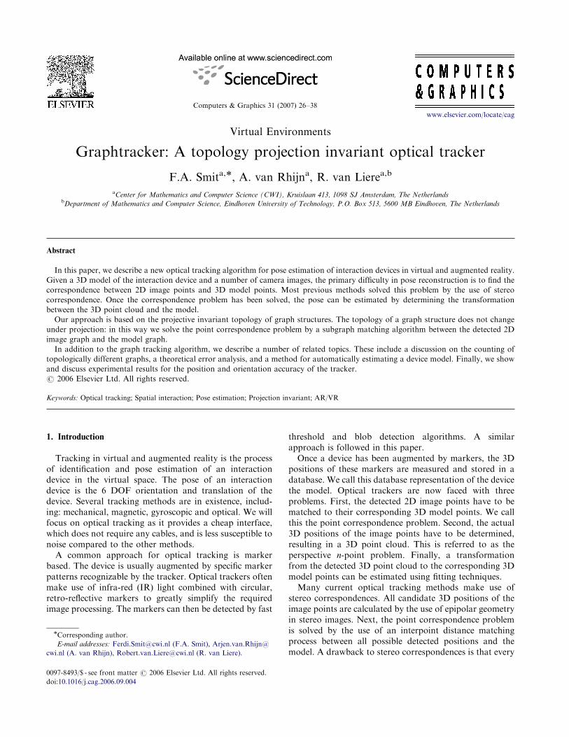
graph. A sample input device is shown in Fig. 1.

The paper is organized as follows. In Section 1.1,

we describe the context in which our tracking method has

been evaluated. In Section 2 we discuss related work. In

Section 3 we give a detailed technical description of our

methods. Section 4 shows experimental results, followed

by a discussion of the pros and cons of the method in

Section 5.

1.1. The Personal Space Station

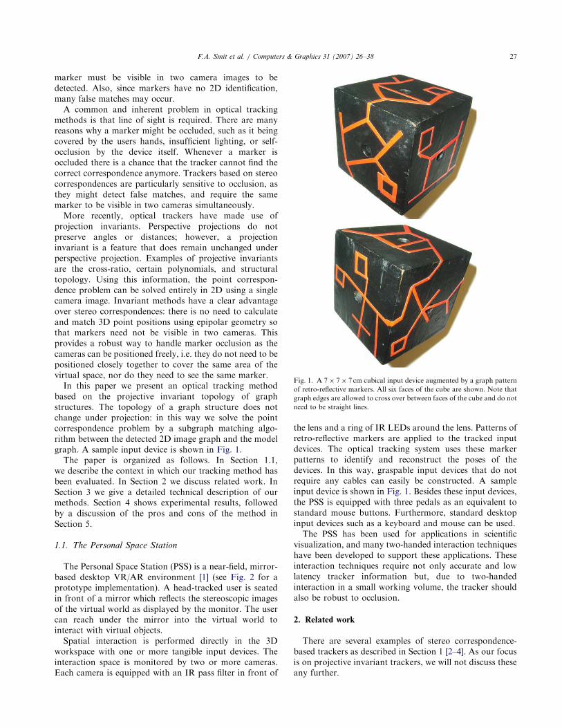
The Personal Space Station (PSS) is a near-field, mirror-

based desktop VR/AR environment [1] (see Fig. 2 for a

prototype implementation). A head-tracked user is seated

in front of a mirror which reflects the stereoscopic images

of the virtual world as displayed by the monitor. The user

can reach under the mirror into the virtual world to

interact with virtual objects.

Spatial interaction is performed directly in the 3D

workspace with one or more tangible input devices. The

interaction space is monitored by two or more cameras.

Each camera is equipped with an IR pass filter in front of

the lens and a ring of IR LEDs around the lens. Patterns of

retro-reflective markers are applied to the tracked input

devices. The optical tracking system uses these marker

patterns to identify and reconstruct the poses of the

devices. In this way, graspable input devices that do not

require any cables can easily be constructed. A sample

input device is shown in Fig. 1. Besides these input devices,

the PSS is equipped with three pedals as an equivalent to

standard mouse buttons. Furthermore, standard desktop

input devices such as a keyboard and mouse can be used.

The PSS has been used for applications in scientific

visualization, and many two-handed interaction techniques

have been developed to support these applications. These

interaction techniques require not only accurate and low

latency tracker information but, due to two-handed

interaction in a small working volume, the tracker should

also be robust to occlusion.

2. Related work

There are several examples of stereo correspondence-

based trackers as described in Section 1 [2–4]. As our focus

is on projective invariant trackers, we will not discuss these

any further.

ARTICLE IN PRESS

Fig. 1. A 7� 7� 7 cm cubical input device augmented by a graph pattern

of retro-reflective markers. All six faces of the cube are shown. Note that

graph edges are allowed to cross over between faces of the cube and do not

need to be straight lines.

F.A. Smit et al. / Computers & Graphics 31 (2007) 26–38 27

A cross-ratio projective invariant of four collinear, or

five coplanar points was used by van Liere et al. [5]. They

use the invariant property to establish pattern correspon-

dence in 2D, as opposed to direct point correspondence.

Once the pattern is identified, the individual points are

matched using a stereo-based distance fit. The matching is

simplified significantly due to the previously established

pattern correspondence.

Van Rhijn [6] used the angular cross-ratio of line pencils

as projective invariant. Once pattern correspondence has

been established, the rotational part of the device pose can

be determined directly by a line-to-plane fitting routine.

The translation still needs to be determined from the

combination of two camera images, however, the same

points need not be visible simultaneously. The method can

handle partial occlusion of the line pencils without

difficulty.

A topological approach is suggested by Costanza et al.

[7]. They make use of region adjacency trees to detect

individual markers. Detection is performed by a subgraph

matching algorithm, which can optionally be made error

tolerant. However, no device pose estimation is performed

in the initial algorithm. An extension was described by

Bencina et al. [8] who determined a 2D translation of

markers on a flat transparent surface. However, their pose

estimation appears sensitive to occlusion. Our method is

somewhat related, especially in the subgraph matching

phase. However, we use actual graphs and are able to

determine a full 6 DOF pose, in addition to being less

sensitive to occlusion.

A widely used framework for augmented VR is

ARToolkit [9]. This system solves pattern correspondence

by detecting a square, planar bitmap pattern. Using image

processing and correlation techniques the coordinates of

the four corners of the square are determined, from which a

6 DOF pose can be estimated. Drawbacks are that

ARToolkit cannot handle occlusion, and only works with

planar markers and four coplanar points. Fiala [10]

handled the occlusion problem by using an error correcting

code as bitmap pattern in ARTag. However, the markers

still need to be planar and the pose is estimated from four

coplanar points. Our method can handle any number of

points in many configurations, for example on a cylinder or

a sphere.

3. Methods

In this section we give a detailed technical description of

our methods. First, we give a description of the graph

tracking algorithm. We then provide a brief mathematical

analysis of the error made in pose estimation, followed by a

discussion on how many topologically different graphs can

be constructed. Finally, we describe a method that allows

us to automatically estimate device models.

3.1. Graph tracking algorithm

The graph tracking algorithm is based on the detection

and matching of graphs to solve the correspondence

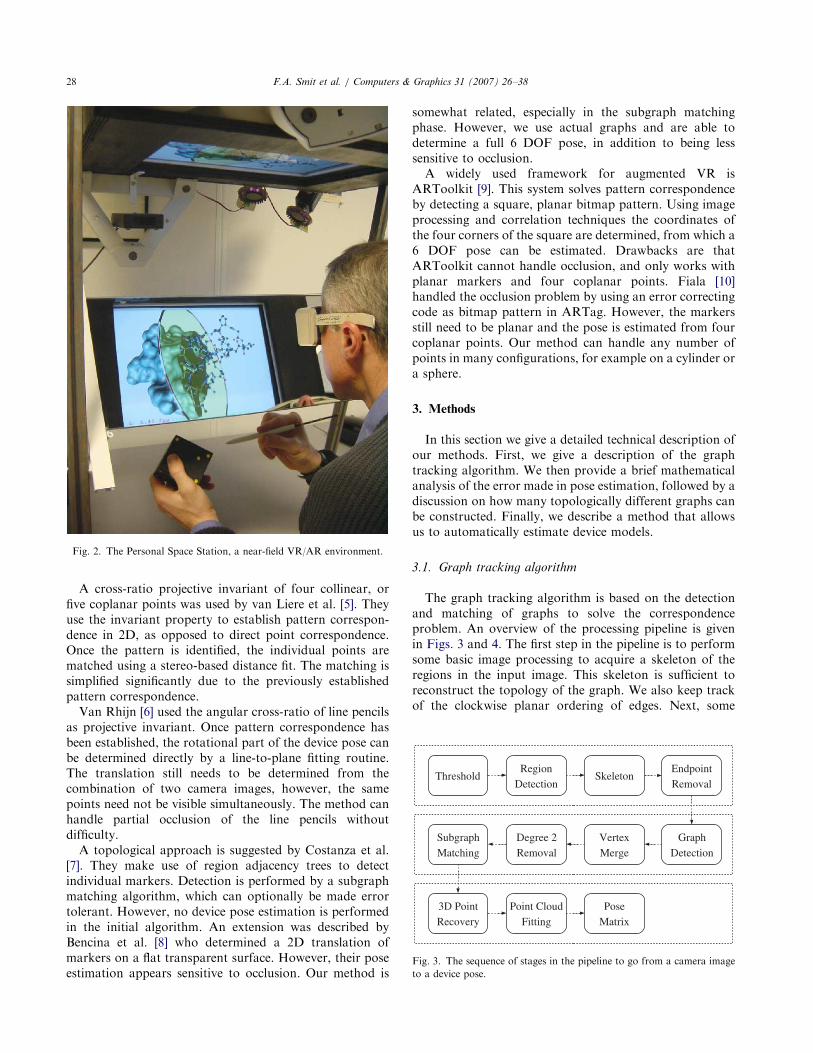
problem. An overview of the processing pipeline is given

in Figs. 3 and 4. The first step in the pipeline is to perform

some basic image processing to acquire a skeleton of the

regions in the input image. This skeleton is sufficient to

reconstruct the topology of the graph. We also keep track

of the clockwise planar ordering of edges. Next, some

ARTICLE IN PRESS

Fig. 2. The Personal Space Station, a near-field VR/AR environment.

Fig. 3. The sequence of stages in the pipeline to go from a camera image

to a device pose.

F.A. Smit et al. / Computers & Graphics 31 (2007) 26–3828

graph simplification is performed to eliminate spurious

edges, followed by the ordered subgraph isomorphism

testing phase to determine correspondence. Image points

are vertices of degree three or greater in the detected graph.

Once we have determined a correspondence between the

image points and the model, a closed-form pose estimation

algorithm is performed. The pose estimation algorithm first

calculates the 3D positions of the image points, followed by

an absolute orientation algorithm to fit the point cloud to

the model and find a transformation matrix. Finally, we

describe an optional iterative solution to the pose estima-

tion problem. The five major stages are each described in a

separate subsection below.

3.1.1. Image processing

Due to the use of retro-reflective markers and IR

lighting, the preliminary image processing stage is straight-

forward. It is divided into four stages: thresholding, region

detection, skeletization, and end-point removal. All stages

use simple algorithms as described by Gonzales and

Woods [11].

First the input image is processed by an adaptive

thresholding algorithm. Next, regions are detected and

merged starting at the points found by thresholding. The

detected regions are processed by a morphology-based

skeletization algorithm. The resulting skeleton suffers from

small parasitic edges, which are removed in the final phase.

The final result is a strictly 4-connected, single pixel width

skeleton of the input regions. This is the basic input to the

graph topology detector.

3.1.2. Graph detection

The graph detector makes some basic assumptions about

the structure of graphs: any pixel that does not have exactly

two neighbours in the skeleton is a vertex, and an edge

exists between any vertices with a path between them

consisting of pixels with exactly two neighbours. The

implications are two-fold. First, edges do not have to be

straight lines; as long as two vertices are connected in some

way there is an edge between them. This means the same

graph can be on arbitrary convex surface shapes. Secondly,

vertices of degree two cannot exist unless there is a self-

loop at the vertex (i.e. a degree one vertex with an extra

self-loop becomes a degree two vertex).

Next, we discuss the algorithm used to detect the graph

topology from a given skeleton image. Suppose we have a

set of vertices V ¼ fvig, and a map Mðx; yÞ ! vi that maps

image coordinates to this set whenever a vertex exists at

that coordinate. The vertex set initially only contains the

(arbitrary) starting point. As long as the set is not empty,

we take a vertex from it and process this vertex as described

in the next paragraph.

Once a starting vertex has been chosen, we start at an

arbitrary neighbour of that vertex and perform a recursive

walk to adjacent pixels. From now on we only consider the

three neighbours of a pixel different from the neighbour we

reached this pixel from. First we consult the map M to see

if this pixel is an existing vertex, and if so, insert an edge.

Also, the pixel is set to zero in the image to indicate it has

been searched. Next, we examine the neighbours of this

pixel. Whenever there is exactly one neighbour, we can

simply ‘walk’ to this neighbour and continue the recursion.

When there are multiple neighbours, the pixel is added to

the vertex set V and an edge is inserted. When there are

zero neighbours an edge is inserted, but the vertex is not

added to the vertex set. After inserting an edge we choose a

new starting vertex from the set V and repeat the

procedure. The process terminates once the set V is

exhausted, at which time the entire topology has been

constructed.

For reasons explained in Section 3.1.3, we impose an

ordering on the incident edges of a vertex. We keep track of

the pixel direction (N,E,S,W) a vertex is left from, and the

direction a vertex is reached from in the recursive walk over

pixels (also see Fig. 5). Every edge now has an ordering

attribute on both ends. We use the starting points of edges

for the ordering instead of the end-points, as end-points

might affect the ordering when occluded. Also note that

this ordering of incident edges is projection invariant up to

cyclic permutations.

Even though small edges were removed from the

skeleton in the image processing phase, it is still possible

for the detected graph to contain very short parasitic edges.

These edges have a harmful effect on our matching

algorithm, and thus they are removed in a subsequent step

ARTICLE IN PRESS

Fig. 4. A schematic visualization of the various stages in converting a

camera image to a graph topology that can be matched (also see Fig. 3).

From top-left to bottom-right the images show a visualization of the state

after: image acquisition, thresholding, region detection, skeletization, end-

point removal, graph detection, short edge removal, degree-two removal,

and graph matching.


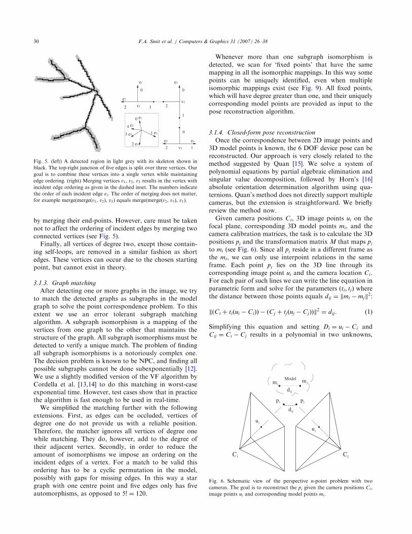
by merging their end-points. However, care must be taken

not to affect the ordering of incident edges by merging two

connected vertices (see Fig. 5).

Finally, all vertices of degree two, except those contain-

ing self-loops, are removed in a similar fashion as short

edges. These vertices can occur due to the chosen starting

point, but cannot exist in theory.

3.1.3. Graph matching

After detecting one or more graphs in the image, we try

to match the detected graphs as subgraphs in the model

graph to solve the point correspondence problem. To this

extent we use an error tolerant subgraph matching

algorithm. A subgraph isomorphism is a mapping of the

vertices from one graph to the other that maintains the

structure of the graph. All subgraph isomorphisms must be

detected to verify a unique match. The problem of finding

all subgraph isomorphisms is a notoriously complex one.

The decision problem is known to be NPC, and finding all

possible subgraphs cannot be done subexponentially [12].

We use a slightly modified version of the VF algorithm by

Cordella et al. [13,14] to do this matching in worst-case

exponential time. However, test cases show that in practice

the algorithm is fast enough to be used in real-time.

We simplified the matching further with the following

extensions. First, as edges can be occluded, vertices of

degree one do not provide us with a reliable position.

Therefore, the matcher ignores all vertices of degree one

while matching. They do, however, add to the degree of

their adjacent vertex. Secondly, in order to reduce the

amount of isomorphisms we impose an ordering on the

incident edges of a vertex. For a match to be valid this

ordering has to be a cyclic permutation in the model,

possibly with gaps for missing edges. In this way a star

graph with one centre point and five edges only has five

automorphisms, as opposed to 5! ¼ 120.

Whenever more than one subgraph isomorphism is

detected, we scan for ‘fixed points’ that have the same

mapping in all the isomorphic mappings. In this way some

points can be uniquely identified, even when multiple

isomorphic mappings exist (see Fig. 9). All fixed points,

which will have degree greater than one, and their uniquely

corresponding model points are provided as input to the

pose reconstruction algorithm.

3.1.4. Closed-form pose reconstruction

Once the correspondence between 2D image points and

3D model points is known, the 6 DOF device pose can be

reconstructed. Our approach is very closely related to the

method suggested by Quan [15]. We solve a system of

polynomial equations by partial algebraic elimination and

singular value decomposition, followed by Horn’s [16]

absolute orientation determination algorithm using qua-

ternions. Quan’s method does not directly support multiple

cameras, but the extension is straightforward. We briefly

review the method now.

Given camera positions Ci, 3D image points ui on the

focal plane, corresponding 3D model points mi, and the

camera calibration matrices, the task is to calculate the 3D

positions pi and the transformation matrix M that maps pito mi (see Fig. 6). Since all pi reside in a different frame as

the mi, we can only use interpoint relations in the same

frame. Each point pi lies on the 3D line through its

corresponding image point ui and the camera location Ci.

For each pair of such lines we can write the line equation in

parametric form and solve for the parameters ðti; tjÞ wherethe distance between those points equals d ij ¼ kmi �mjk2:

kðCi þ tiðui � CiÞÞ � ðCj þ tjðuj � CjÞÞk2 ¼ d ij . (1)

Simplifying this equation and setting Di ¼ ui � Ci and

Cij ¼ Ci � Cj results in a polynomial in two unknowns,

ARTICLE IN PRESS

Fig. 5. (left) A detected region in light grey with its skeleton shown in

black. The top-right junction of five edges is split over three vertices. Our

goal is to combine these vertices into a single vertex while maintaining

edge ordering. (right) Merging vertices v1, v2, v3 results in the vertex with

incident edge ordering as given in the dashed inset. The numbers indicate

the order of each incident edge ei. The order of merging does not matter,

for example merge(merge(v1, v2), v3) equals merge(merge(v2, v3), v1).

Fig. 6. Schematic view of the perspective n-point problem with two

cameras. The goal is to reconstruct the pi given the camera positions Ci,

image points ui and corresponding model points mi .


(ti, tj), with the following coefficient matrix:

�d ij þ Cij � Cij �2ðDj � CijÞ Dj �Dj

2ðDi � CijÞ �2ðDi �DjÞ 0

Di �Di 0 0

0

B

@

1

C

A. (2)

Every pair of points defines an equation of this form.

However, solving such a system of non-linear equations

algebraically proves extremely difficult. A direct solution

can be obtained using Grobner bases, however, the number

of terms in this solution is extremely large and it is sensitive

to numerical errors.

We can simplify the coefficient matrix greatly by

normalizing the direction vectors of the parametric lines

(Di �Di ¼ Dj �Dj ¼ 1) and translating all cameras to the

same point at the origin (Cij ¼ 0). Once these simplifica-

tions have been made, the polynomial system reduces to

the same form as defined by Quan [15]:

Pij ¼ t2i þ t2j � 2ðDi �DjÞ � d ij ¼ 0. (3)

Because of the simplifying camera translations, the new

distance calculation becomes

d ij ¼ kðmi � CiÞ � ðmj � CjÞk2 ¼ kmi �mj :� Cijk2. (4)

Given N input points, there are N2

� �

constraining

equations. Using three equations Pij ;Pik;Pjk in ti; tj ; tk we

can construct a fourth degree polynomial in t2i by variable

elimination. If we fix the first parameter to ti, we can

construct N�12

� �

such polynomials in t2i . For N44 this

system is an over defined linear system in

ð1; t2i ; ðt2i Þ2; ðt2i Þ3; ðt2i Þ4Þ, which can be solved in a least-

squares fashion by using a singular value decomposition on

a N�12

� �

� 5 matrix. In the case of N ¼ 4 a slight

modification has to be made, as the linear system is under

determined in this case, but a unique solution can still be

found (see [15] for details). This means we need to detect a

minimum of four points over all the cameras to reconstruct

the 3D point cloud.

Note that after calculating ti we cannot simply substitute

its value in the original polynomial equations. As the

obtained solution is a least-squares estimate, there might

not exist a solution to the polynomial equation using this

variable. Recall that the polynomial equation represents a

constraint on the distance between two lines. By fixing a

point on one of these lines, there is no guarantee that there

even exists a point on the other line for which the distance

constraint holds. One could minimize the difference in

distance, however, to be precise all points need to be taken

into account. Therefore, we simply solve all of the tiseparately using the method described above.

At this point we have effectively solved the least-squares

perspective n-point problem for multiple cameras in closed

form. The next step is to determine a transformation

matrix between the determined 3D point cloud and the 3D

model. To accomplish this we use the closed-form absolute

orientation method from Horn [16]. As this algorithm can

be left unmodified we will not describe it any further here.

3.1.5. Iterative pose reconstruction

Occasionally the closed-form perspective n-point algo-

rithm for multiple cameras fails to find a reliable pose. This

could be caused by a number of factors, such as slight

errors in the device model description, camera noise,

numerical instability and near-critical configurations. In an

attempt to partially overcome these problems we applied

an iterative pose estimation algorithm as described by

Chang and Chen [17]. The iterative algorithm can be seen

as an optional post-processing step to enhance the

reliability of the solution. The accuracy of the solution is

not greatly affected, as the closed-form algorithm already

provides a least-squares solution.

The iterative algorithm relies on an initial pose M0,

which we provide either as the solution of the perspective n-

point problem, or as the device pose estimated in the

previous frame. Once an initial pose is given, the 3D model

points mi are transformed back to camera space. Now two

possibilities occur for these transformed points pti :

� The point pti is visible in multiple cameras. In this case

we can determine a desired point location ppi by finding

the best intersection of all the camera rays through

corresponding 3D camera points ui on the focal plane.

� The point pti is visible in only one camera. Now we can

find the desired point location ppi by a perpendicular

projection of the transformed point on the correspond-

ing camera ray.

Once the sets fptig and fppi g of transformed and desired

point locations are known, a least-squares rigid transfor-

mation M� between the two sets can be determined using

Horn’s method [16]. This transform M� can be seen as an

error measure of the initial pose. The procedure can be

repeated by setting the new initial pose to Mn ¼ M��Mn�1.

The algorithm terminates when M� is sufficiently close to

identity.

3.2. Error analysis

Next, we will describe a mathematical model of the

errors made in pose estimation under the presence of noise,

using multiple cameras. We can distinguish between three

sources of errors: inaccurate vertex positions in the camera

images, errors in the device description, and errors in the

camera calibration. For our purposes we only consider the

first source of errors, and assume both the device as well as

the camera errors to be negligible.

As depth information cannot be obtained by using a

single projected point, we assume a camera with two

detected points as shown in Fig. 7. If we assume the error

in the projected image points to follow a Gaussian

distribution with expectation �b, the resulting expected

errors �XY in the XY-, and �Z in the Z-direction are given by

�XY ¼ d

f�b; �Z ¼ d2

�b

lf � d�b, (5)

ARTICLE IN PRESS


where d is the distance from the points to the camera’s centre

of projection, f the focal distance, and l the distance between

the points. Note that �Z is larger than �XY , and thus the

largest error is made in estimating depth information.

Extending equation (5) to N points results in

�NXY ¼ 1

ffiffiffiffiffi

Np �XY ; �

NZ ¼ 1

ffiffiffiffiffi

Np �Z. (6)

Eq. (6) shows that the error decreases in all directions

when more points are visible to the camera. We can extend

these equations to the case of multiple cameras. To do this,

the expectations have to be transformed to a common

reference frame. Writing Nc for the number of cameras, and

�i for the transformed expectation of errors in the ith camera

gives

� ¼ 1

Nc

ffiffiffiffiffiffiffiffiffiffiffi

X

i

�i

r

(7)

for each of the three directions with respect to the reference

frame. Eq. (7) shows that the expected error is reduced by

increasing the amount of cameras. Our initial claim to use

multiple cameras in our method to reduce the amount of

error in pose estimation is supported by this result.

3.3. Graph counting

As discussed previously, to solve the point correspon-

dence and identification problem we rely on subgraph

matching. In order to find a unique match between a

smaller subgraph and the model graph, there must not be

more than one subgraph in the model with the same

topological structure. Also, the (sub)graph itself should not

be automorphic, as it prevents us from identifying vertices

uniquely. This raises the question of exactly how many

topologically different graphs we can construct, and thus

the extensibility of our system.

Some of these graph counting questions are still

unanswered in the field of mathematics, and, therefore,

we cannot give an exact answer to the extensibility

question. However, we can investigate similar known

counting problems to give a good indication. One of these

is the number of topologically different planar graphs given

a fixed number of vertices. Our model graph is not

necessarily planar, but it will always be locally planar as

it is mapped on a tangible convex input device and edges

cannot cross without intersecting. Therefore, the number of

planar graphs serves as an indication of the extensibility

and is given in Table 1.

It can be seen that the number of graphs explodes for

seven vertices or more. Our algorithm requires the vertices

used for pose estimation to be of degree at least three;

however, this does not imply that for graph construction all

vertices are necessarily of degree three or more. We can use

extra vertices of degree one or more to aid in constructing

different topologies. Nonetheless, even for graphs having

only vertices of degree three or more, there are many

topologically different graphs from 7–8 vertices onward

(see Table 1).

There are two more properties of our algorithm that

provide us with even more graphs to choose from. First,

even though vertices with degree zero are not allowed,

loops on vertices are allowed. The existence of loops can be

seen as somewhat equivalent to removing the constraint

that vertices have degree at least one in a counting

argument. This means that the number of graphs to choose

from is closer to the first row of Table 1.

Secondly, by using the imposed planar ordering as

described in Section 3.1.3, we can distinguish between

graphs that would otherwise be topologically equivalent.

The ordering of edges reduces the search space for graph

matching by increasing the number of topologically

different graphs.

Finally, it should be noted that not all topologically

different graphs are equally good choices. The distance

between two graphs is often defined as the number of graph

edit operations required to transform one graph into the

other. To allow for better detection and occlusion handling

we would prefer graphs with a large distance to each other.

Determining the distance between two graphs is often a

complex problem by itself (e.g. [18]). Therefore, counting

the number of non-isomorphic graphs with maximum

distance would be a difficult problem and to the best of our

knowledge has not been solved. One useful approach for

future work might be to use some graph representation of

ARTICLE IN PRESS

Fig. 7. Expected error perpendicular to the camera plane.

Table 1

Number of topologically different planar graphs using a fixed amount of

vertices of degree at least n

Degree X Number of vertices

1 2 3 4 5 6 7 8 9 10

0 1 2 4 11 33 142 822 6966 79 853 1 140 916

2 0 0 1 3 10 50 335 3194 39 347 579 323

3 0 0 0 1 2 9 46 386 3900 48 766

4 0 0 0 0 0 1 1 4 14 69


an error correcting code, as these codes follow strict

distance criteria.

3.4. Model estimation

Our graph topology-based tracking method requires a

model that describes the graph topology of the markers on

the device, along with the 3D locations of the graph

vertices in a common frame of reference. Creating such a

model by hand is a tedious and error prone task, and is

only possible for simple shaped objects.

Van Rhijn and Mulder [4] presented a method for

automatic model estimation from motion data, using

devices equipped with point shaped markers. When a

new device is constructed, a user moves it around in front

of the cameras, showing all markers. The system incremen-

tally updates a model that describes the 3D marker

locations in a common frame of reference. This enables a

user to quickly construct new interaction devices and create

accurate models. As a result, the flexibility and robustness

of the tracking system is greatly increased.

These techniques can be adapted to automatically

estimate a model needed for our graph topology-based

optical tracker. Two methods are developed that differ in

the amount of information that has to be specified

manually. The first method is a fully automatic model

estimation method, where no prior information about the

interaction device is required. The aim is to obtain a model

that describes the graph topology and 3D vertex locations.

In the second case, the graph topology has to be

prespecified in an abstract form. The aim is to obtain a

model describing the 3D vertex locations, which are needed

for pose estimation. This approach greatly simplifies the

model estimation procedure and makes it more robust. In

the next sections, both methods will be described in more

detail.

3.4.1. Fully automatic model estimation

When the graph topology is unknown, two cameras are

needed to determine the 3D locations of graph vertices.

The model estimation procedure is then a straightforward

extension of the method presented in [4]. The method

proceeds as follows. First, stereo correspondence is used to

obtain the 3D locations of the graph vertices. Next, frame-

to-frame correspondence is exploited to assign a unique

identifier to each vertex during the time it is visible. A

graph G ¼ ðV ;P;D;E;OÞ is maintained, where

� V is a set of vertices vi.

� P � V is a set of 3D locations, where pi assigns a 3D

location to vertex vi in a common frame of reference.

� D � V � V is a set of distance edges, where d ij

represents the average Euclidean distance between

vertices vi and vj. A distance edge d ij is only present if

it remains static during motion.

� E � V � V is a set of edges, where an edge eij is only

present if vi and vj have a connecting marker path.

� O � V � V is an edge ordering, where oij assigns a

planar ordering index to edge eij with respect to vertex

vi, in clockwise fashion.

The procedure starts by adding all visible vertices to G.

The distances d ij are determined, and the camera images

are analysed to determine if visible vertex pairs (vi, vj) are

connected. If so, edges eij are created. As vertices are

moved around, the Euclidean distance between each vertex

pair is examined and compared to the distance d ij in G. If

the difference in distances exceeds a certain threshold, the

distance edge d ij is deleted.

When a vertex appears for which no frame-to-frame

correspondence can be determined, the system needs to

distinguish between a new vertex appearing and a

previously occluded vertex reappearing. This is accom-

plished by predicting the location of all occluded vertices of

the model. The graph G stores a model of all 3D vertex

locations in a normalized coordinate system, giving the set P.

Vertex locations are averaged over all frames to reduce

inaccuracies due to noise and outliers. The locations can be

determined by calculating the rigid body transform that

maps the identified vertices to the corresponding model

vertices in a least-squares manner [16]. This transform is

used to predict the locations of occluded vertices. When a

vertex is found for which no frame-to-frame correspon-

dence could be established, its location is compared to the

predicted occluded vertex locations. If the vertex is

classified as new, it is added to the graph, and distance

edges d ij are created to connect it to the visible vertices.

Each frame, the camera images are examined to

determine if vertices vi and vj have a connecting marker

path. To handle temporary occlusion of the marker paths

between vertices, an edge eij is only removed from the

graph if there is enough evidence to do so. For each edge

eij, an edge ordering oij is maintained with respect to vertex

vi (see Section 3.1.2).

Due to possible inaccuracies in the stereo correspon-

dence method, false 3D vertex locations may appear in the

motion data. To reduce the probability that these are

included in the model, a pyramid-based clustering of the

graph G is performed with respect to the distance edges d ij,

which finds all rigid subgraphs. Pyramids or 4-cliques are

detected in G, and are considered to be connected if they

share a triangle. Clusters are defined by the connected

components of the pyramid graph. Although connected

pyramids do not necessarily form a clique, vertices within a

cluster are part of the same rigid structure. The rigid body

transform of each cluster is computed using the visible

vertices, and used to predict the location of the occluded

vertices. Note that this also allows for simultaneous model

estimation of multiple objects.

3.4.2. Model estimation with specified graph topology

When the graph topology is given, the model estimation

procedure as detailed in the previous section can be greatly

simplified. In this case, the only unknown in the model

ARTICLE IN PRESS


graph GT is the set of 3D vertex locations P. Since the

topology is given, the graph matching techniques described

in Section 3.1.2 can be applied to find a subgraph in each

camera image. Therefore, graph vertices are uniquely

identified in 2D. If a vertex is visible in at least two

cameras, simple epipolar geometry can be used to obtain its

3D location.

As a consequence, the model estimation procedure is

greatly simplified and more robust. Stereo correspondence,

which is complicated and can result in invalid 3D vertex

locations, is not needed. Since the vertex identification is

already known in 2D, frame-to-frame correspondence and

occluded vertex location prediction are also not required.

The clustering step, which is used to identify false 3D

vertex locations and to distinguish between vertices from

different objects, can be omitted. The data that is used to

update the model graph is reliable, and the vertex

identification determines which vertices belong to which

object. This reduces the model estimation procedure to

expressing the identified 3D vertex locations in a common

frame of reference throughout the motion sequence.

4. Results

Our implementation uses a cubical input device aug-

mented by retro-reflective markers, as shown in Fig. 1.

Fig. 8 shows a practical example of the image processing

pipeline, which has been shown schematically in Figs. 3

and 4 earlier. A captured camera image is shown, followed

by some steps required to perform graph detection. A

number of steps, such as end-point removal and vertex

merge, have been omitted.

In the presence of occlusion, several points can still be

uniquely identified, allowing the device pose to be

reconstructed. A few practical examples of occlusion

handling are shown in Fig. 9. Also, using multiple cameras

increased the number of detected points as expected.

The implementation uses relatively unoptimized image

processing algorithms, and runs entirely on the CPU. Even

so, the entire reconstruction, from image processing to pose

estimation with multiple cameras, takes between 10 and

20ms per frame. Of this time more than half is spent in the

unoptimized image processing phase. These results show

that our method is well suited to run in real-time with

multiple cameras.

4.1. Tracking accuracy

Determining the absolute accuracy of a tracker over the

entire working volume is a tedious and time-consuming

process. A grid of sufficient resolution covering the

tracking volume has to be determined. Next, the device

has to be positioned accurately at each grid position, and

the resulting tracker measurement has to be determined.

We have used a different, simplified approach to measure

the accuracy of both the reported position and orientation.

Measurements were made in the following ways:

ARTICLE IN PRESS

Fig. 8. A number of processing steps performed to match a graph in a

camera image. (top left) A raw image as captured by our infra-red

cameras. (top right) The resulting image after thresholding and region

detection. (bottom left) The result of running a skeletization algorithm.

(bottom right) The detected graph after reading and matching the graph

from the skeletized image. Five unique points are identified.

Fig. 9. When parts of the graph are occluded, some fixed points can still

be detected. An interesting example is the bottom-right image; the detected

subgraph matches the model in two ways. The point connecting the two

self-loops can be uniquely identified by noting a fixed point. However, the

points representing the loops themselves cannot be uniquely identified as

the two points can be interchanged freely.


� Position accuracy was measured by sliding the device

over a plane of constant height in the tracking volume

and logging the positional result. Thus, the measured

device positions should all lie on the XZ-plane. Now we

determine the average distance to the XZ-plane, which

gives an indication of the systematic error made. The

standard deviation of this set of distances (RMSE) gives

a good indication of the random error.

� Orientation accuracy was also measured by sliding the

device over a fixed plane; however, this time we

measured the angle between a device axis perpendicular

to the plane and the plane normal. Thus, ideally the

measured angles are equal to zero. Again the average

and standard deviation of this set give good indications

for the systematic and random error.

Although this procedure does not provide us with an

absolute accuracy, we do get relative accuracy with respect

to the plane. The results of the XZ-plane measurements for

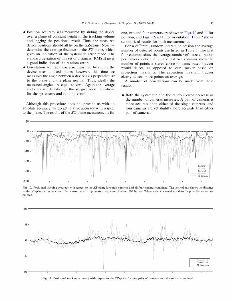
one, two and four cameras are shown in Figs. 10 and 11 for

position, and Figs. 12and 13 for orientation. Table 2 shows

summarized results for both measurements.

For a different, random interaction session the average

number of detected points are listed in Table 3. The first

four columns show the average number of detected points

per camera individually. The last two columns show the

number of points a stereo correspondence-based tracker

would detect, as opposed to our tracker based on

projection invariants. The projection invariant tracker

clearly detects more points on average.

A number of observations can be made from these

results:

� Both the systematic and the random error decrease as

the number of cameras increases. A pair of cameras is

more accurate than either of the single cameras, and

four cameras are yet slightly more accurate than either

pair of cameras.

ARTICLE IN PRESS

20

0

-20

-40

-60

-80

-100

Camera 1

Camera 2

Camera 3

Camera 4

All Cameras

Fig. 10. Positional tracking accuracy with respect to the XZ-plane for single cameras and all four cameras combined. The vertical axis shows the distance

to the XZ-plane in millimeters. The horizontal axis represents a sequence of about 200 frames. When a camera could not detect a pose the values are

omitted.

10

5

0

-5

-10

Camera 1/2

Camera 1/2

All Cameras

Fig. 11. Positional tracking accuracy with respect to the XZ-plane for two pairs of cameras and all cameras combined.


� In the case of cameras 1 and 2, the XZ-plane is almost

parallel to the camera planes. In this case the error is

mostly determined by the depth estimation. Hence, the

error is dominated by �Z as given in Eq. (5). For cameras

3 and 4 the XZ-plane is at a near 45� angle, and thus the

systematic error is decreased as can be seen in Table 2.

However, the random error is increased as the cameras

are positioned further away. The combination of all

cameras is even more accurate as the device is viewed

from more directions now.

� The total number of detected points increases as the

number of cameras increases. Hence, a pose can be

determined a larger percentage of the time with more

cameras. The theoretical accuracy is increased as well,

since more points are being used in the calculations.

Stereo correspondence can often not be found, while

ARTICLE IN PRESS

40

30

20

10

0

-10

-20

-30

Camera 1

Camera 2

Camera 3

Camera 4

All Cameras

Fig. 12. Angular tracking accuracy with respect to the XZ-plane for single cameras and all four cameras combined. The vertical axis shows the angle with

the XZ-plane in degrees. The horizontal axis represents a sequence of frames.

Camera 1/2

Camera 3/4

All Cameras

15

10

5

0

-5

-10

-15

Fig. 13. Angular tracking accuracy with respect to the XZ-plane for two pairs of cameras and all cameras combined.

Table 2

Measurement-to-plane summarized results for 1/2/4 cameras

Camera Positional accuracy (in mm) Angular accuracy (in degrees)

Average RMSE Average RMSE

1 �26.4 15.4 14.3 6.67

2 �25.1 15.3 �8.4 4.36

3 �12.7 10.8 0.99 7.15

4 �20.5 24.3 �9.9 3.27

1/2 0.232 0.90 0.82 3.41

3/4 �0.0754 2.01 0.14 1.69

1/2/3/4 0.0324 0.57 �0.3 1.08

The average distance to the XZ-plane and the RMSE are given in the first

two columns. The average angle with the plane and corresponding RMSE

are given in the last two columns.

Table 3

Average number of detected unique points for single cameras, stereo and

projection invariant tracking during a random interaction session

Camera 1 2 3 4 Stereo Invariant

Points 4.7 4.9 5.1 4.7 5.7 7.8


individual cameras do see enough points combined for

pose reconstruction.

� Occasionally a single camera reports a better pose than a

combination of cameras. This is usually caused by one

of the other cameras reporting a very inaccurate pose.

Also, camera 3 seemingly reports a very good pose as

the average angle is very close to zero. However, the

standard deviation is fairly high, indicating an unreliable

pose. For accurate, robust tracking the combination of

both a low average and standard deviation is important.

5. Discussion

To allow for robustness against occlusion, it is important

that a detected, occluded subgraph can be matched to a

unique subgraph in the model. However, it is not yet

completely clear what kind of graph topology is best suited

to accomplish this. We found through direct experimenta-

tion that model graphs consisting of several ordered non-

isomorphic components are desirable. Also, each of the

components, and the entire model itself, should not be

ordered automorphic (except for the trivial identity

mapping).

A different approach would be to extend the graph

matching algorithm to detect missing vertices and edges

due to common cases of occlusion. However, developing a

matching algorithm that incorporate this kind of meta-

knowledge and still runs in real-time might be infeasible.

We can also impose the requirement that all model graphs

must be planar or locally planar, which allows the use of

much faster graph matching algorithms [12]. This might,

however, affect the types of (convex) surfaces we can use

for devices.

Another issue is the optimal placement of cameras. We

expect a camera setup with three cameras, one on each

principal axis, will be optimal with respect to the error

made in pose estimation (see Section 3.2), however, this has

still to be verified formally. Also, by varying camera

placements, occlusion by the users hands might be avoided

entirely as one side of the input device might always be

completely visible.

So far we have only used our algorithm in an outside-to-

inside setting for device tracking in AR/VR. However, this

is not a limitation and the algorithm could be used in an

inside-to-outside setting as well. A possible alternative

application of the tracker is locating a camera using a large

fixed model graph and a moving camera. Another

application could be the detection and tracking of markers,

similar to systems such as ARToolkit [9]. Finally, the

tracker can be used to calibrate multiple cameras. As the

2D point correspondences are known, we can determine

the camera matrices and 3D point positions by existing

projective reconstruction algorithms, such as bundle

adjustment [19]. We can then further constrain the solution

by making use of the 3D model description.

Future work will consist of finding more specific

statistical models of camera errors, thereby allowing an a

priori Bayesian estimation of point positions. This will also

provide a starting point for determining optimal camera

locations and angles with respect to accuracy. Also,

developing a more robust graph matching algorithm with

knowledge of occlusion cases might be desirable, as well as

gaining more knowledge about non-isomorphic maximum

distance graphs. Finally, runtime performance with respect

to latency should be evaluated. To increase runtime

performance some of the used algorithms might have to

be modified to run on the GPU.

6. Conclusion

We have proposed a projective invariant optical tracker

based on graph topology. There are four advantages to our

method. First, the correspondence problem is solved

entirely in 2D and, therefore, no stereo correspondence is

needed. Consequently, we can use any number of cameras,

including a single camera. Secondly, as opposed to stereo

methods, we do not need to detect the same model point in

two different cameras, and, therefore, our method is more

robust against occlusion. Thirdly, the subgraph matching

algorithm can still detect a match even when parts of the

graph are occluded, for example by the users hands. This

also provides more robustness against occlusion. Finally,

the error made in the pose estimation is significantly

reduced as the amount of cameras is increased.

A number of additional topics were discussed. We have

shown a theoretical analysis of the errors made in

estimating a device pose, followed by experimental results

supporting this theory. For the construction of devices we

discussed the extensibility of our graph structures by

counting the number of topologically different graphs. As

describing a device model manually is tedious and error

prone, we have also described a method to automatically

estimate a device model. Finally, even though theoretically

complex algorithms are used, the solution is fast enough to

estimate a pose from multiple cameras in real-time.

References

[1] Mulder JD, van Liere R. The Personal Space Station: bringing

interaction within reach. In: VRIC conference proceedings 2002.

p. 73–81.

[2] Dorfmuller K. Robust tracking for augmented reality using retro-

reflective markers. Computers and Graphics 1999;23(6):795–800.

[3] Ribo M, Pinz A, Fuhrmann A. A new optical tracking system for

virtual and augmented reality applications. In: Proceedings of the

IEEE instrumentation and measurement technical conference 2001.

p. 1932–36.

[4] van Rhijn A, Mulder JD. Optical tracking and calibration of tangible

interaction devices. In: Proceedings of the immersive projection

technology and virtual environments workshop, 2005. p. 41–50.

[5] van Liere R, Mulder JD. Optical tracking using projective invariant

marker pattern properties. In: VR ’03: proceedings of the IEEE

virtual reality, 2003. p. 191–8.

[6] van Rhijn A, Mulder JD. Optical tracking using line pencil fiducials.

In: Proceedings of the eurographics symposium on virtual environ-

ments, 2004. p. 35–44.

ARTICLE IN PRESS


[7] Costanza E, Robinson J. A region adjacency tree approach to the

detection and design of fiducials. In: VVG, 2003. p. 63–9.

[8] Bencina R, Kaltenbrunner M, Jorda S. Improved topological fiducial

tracking in the reactivision system. In: CVPR ’05: proceedings of the

IEEE computer society conference on computer vision and pattern

recognition—workshops, 2005. p. 99.

[9] Kato H, Billinghurst M. Marker tracking and hmd calibration for a

video-based augmented reality conferencing system. In: IWAR ’99:

proceedings of the second IEEE and ACM international workshop

on augmented reality, 1999. p. 85–94.

[10] M. Fiala. ARTag, a fiducial marker system using digital techniques.

In: CVPR, vol. 2. 2005. p. 590–6.

[11] Gonzalez RC, Woods RE. Digital image processing. 2nd ed.

Englewood Cliffs, NJ: Prentice-Hall; 2002 ISBN: 0201180758.

[12] Eppstein D. Subgraph isomorphism in planar graphs and related

problems. Journal of Graph Algorithms and Applications

1999;3(3):1–27.

[13] Cordella LP, Foggia P, Sansone C, Vento M. An efficient algorithm

for the inexact matching of arg graphs using a contextual

transformational model. In: ICPR’96: Proceedings of the interna-

tional conference on pattern recognition, vols. III–7276. 1996.

p. 180–4.

[14] Cordella LP, Foggia P, Sansone C, Vento M. A (sub)graph

isomorphism algorithm for matching large graphs. IEEE Transac-

tions on Pattern Analysis and Machine Intelligence

2004;26(10):1367–72.

[15] Quan L, Lan Z. Linear n-point camera pose determination. IEEE

Transactions on Pattern Analysis and Machine Intelligence

1999;21(8):774–80.

[16] Horn B. Closed-form solution of absolute orientation using unit

quaternions. Journal of the Optical Society of America A 1987;4(4):

629–42.

[17] Chang W-Y, Chen C-S. Pose estimation for multiple camera systems.

In: ICPR, vol. 3. 2004. p. 262–5.

[18] Kubicka E, Kubicki G, Vakalis I. Using graph distance in object

recognition. In: CSC ’90: proceedings of the ACM annual conference

on cooperation, 1990. p. 43–8.

[19] Hartley RI, Zisserman A. Multiple view geometry in computer vision.

2nd ed. Cambridge: Cambridge University Press; 2004

ISBN: 0521540518.

ARTICLE IN PRESS


virtual environments graphtracker: a topology projection

Documents