Analysis of I-shape beam to CHS column connection with and without filled of concrete Laura Serra Tojo

VILNIUS GEDIMINAS TECHNICAL UNIVERSITY

FACULTY OF CIVIL ENGINEERING

DEPARTMENT OF STEEL AND TIMBER STRUCTURES

Vilnius, 2017

Professor: Antanas Šapalas

1

Contents ABSTRACT ...................................................................................................................................... 2

PREAMBLE ..................................................................................................................................... 3

Keywords ................................................................................................................................... 3

Major symbols ........................................................................................................................... 3

LIST OF FIGURES ............................................................................................................................ 4

LIST OF TABLES .............................................................................................................................. 5

LIST OF GRAPHS ............................................................................................................................. 6

1 INTRODUCTION ..................................................................................................................... 8

Research object ......................................................................................................................... 8

Research of objectives .............................................................................................................. 8

Tasks research ........................................................................................................................... 8

Research methods ..................................................................................................................... 8

2. THEORETICAL BASIS OF COMPOSITE COLUMNS ................................................................... 9

2.1 Behaviour peculiarities of composite columns ........................................................... 11

2.1.1 Axial compression ............................................................................................... 14

2.1.2 Compression and bending ................................................................................... 18

2.1.2.1 Uniaxial bending and compression ................................................................. 19

2.1.2.2 Biaxial bending and compression .................................................................... 20

2.1.2.3 Simplified determination of bending moments .............................................. 21

2.2 Component method for design of steel joint connections ......................................... 21

2.2.1 Welded joints ...................................................................................................... 22

2.2.2 Bolted joints ........................................................................................................ 24

2.2.3 Hollow section joints ........................................................................................... 29

2.3 Component method for design of composite joint connections ................................ 33

3 PRACTICAL APPLICATION .................................................................................................... 37

3.1 Design of the joint ....................................................................................................... 37

3.2 Analytical calculations ................................................................................................. 40

3.2.1 Buckling calculation ............................................................................................. 40

3.2.1.1 Steel column ........................................................................................................ 41

3.2.1.2 Composite column .............................................................................................. 41

3.2.2 Joint calculation ................................................................................................... 48

3.2.2.1 Steel column ........................................................................................................ 48

3.2.2.2 Composite column .............................................................................................. 53

3.3 Numerical modelling ................................................................................................... 55

3.3.1 Buckling modelling .............................................................................................. 55

2

3.3.1.1 Steel column ........................................................................................................ 55

3.3.1.2 Composite column .............................................................................................. 56

3.3.2 Joint modelling .................................................................................................... 58

3.3.2.1 Steel modelling .................................................................................................... 58

3.3.2.2 Concrete modelling ............................................................................................. 60

3.3.2.3 Geometry ............................................................................................................ 63

3.3.2.4 Finite Element Mesh ........................................................................................... 64

3.3.2.5 Loading and Boundary Conditions ...................................................................... 66

3.3.2.6 Results ................................................................................................................. 67

3.3.2.6.1 Steel joint .................................................................................................. 67

3.3.2.6.2 Composite joint ......................................................................................... 69

4 COMPARISON OF NUMERICAL MODELING AND ANALYTICAL CALCULATIONS RESULTS ... 72

4.1 Bucking comparison .................................................................................................... 72

4.2 Joint comparison ......................................................................................................... 72

4.2.1 Steel column ........................................................................................................ 72

4.2.2 Composite column .............................................................................................. 74

5 COMPARISON OF STEEL COLUMN AND CONCRETE COLUMN ............................................ 77

6 CONCLUSIONS AND PROPOSALS ......................................................................................... 78

7 REFERENCES ........................................................................................................................ 80

ABSTRACT It is thought that the earliest practice of civil engineering may have commenced in ancient Egypt

(4000 and 2000 BC) when the humans started to abandon a nomadic live to stay on the same

place for live, that means that civil engineering is a science that has been studied more than

5000 years. Even so, nowadays there are many fields to investigate and study. Not everything is

known.

This thesis was thought to study a topic that nowadays is not reflected on the regulations. This

theme is the connection between steel beams and composite columns.

This thesis starts with theoretical concepts, the review and analysis of the composite structures

and steel and composite joints. This first part was made with the basis of Eurocode and Design

Guide. After this first theoretical part the practical part starts; this part is based on the

comparison of two types of connections, two connections that are equal CHS column joint with

an I-Beam, but one of the connection the CHS is filled of concrete. The analysis of the

connections was done by hand, all the calculation than could made with Eurocode, and following

with a finite elements study, with the support of the ANSYS program.

To sum up, the thesis was finished with the comparison of both types of joints to solve questions

like: which are the benefits of infill concrete on behaviour of joint? How much load can support?

...

3

PREAMBLE

Keywords Bucking; CHS (Circular Hollow Section); Concrete C25/30; Concrete-filled steel tubular; Fin plate;

I-Beam; Simple shear connection; Steel S275.

Major symbols a Effective throat of weld I Inertia Aa Steel area Ia Steel inertia Ac Concrete area Ic Concrete inertia Ant Area subjected to tension Is Reinforcement inertia Anv Area subjected to shear Lcri Critical length of Euler As Reinforcement area M Bending moment Av Shear area of element My,Sd Bending moment action on y axis d Diameter My,Sd Bending moment resistance on y axis d0 Hole diameter Mpl,y,Rd Plastic bending moment resistance on y axis dc Diameter column Mpl,Rd Plastic bending moment resistance E Elastic young modulus Mpl,z,Rd Plastic bending moment resistance on z axis e Eccentricity MRd Bending moment resistance e1 End distance Mz,Sd Bending moment resistance on z axis e2 Edge distance n Total number of bolts Ea Elastic young modulus steel Ncr Critical axis load of Euler Ɛc Concrete strain NG,Sd Permanent axis load

Ɛc1 Maximum concrete elastic strain schematic curve

Npl,Rd Plastic axis resistance

Ɛc2 Maximum concrete elastic strain parabola-rectangle curve

NRd Axis resistance

Ɛc3 Maximum concrete elastic strain bi-linear curve

NSd Acting design normal force

Ecm Elastic young modulus concrete p1 Distance between holes on load direction

Ɛcu1 Maximum concrete plastic strain schematic curve

p2 Distance between holes perpendicular load direction

Ɛcu2 Maximum concrete plastic strain parabola-rectangle curve

Pcri Critical load of Euler

Ɛcu3 Maximum concrete plastic strain bi-linear curve

Rd Resistance

Es Elastic young modulus refoircement Sd Action Et Elastic young modulus total t Thickness F Tying force or resistance tc Thickness column Fb,Rd Bearing resistance V Shear fcd Concrete strength with security factor β Correlation factor fck Concrete strength βw Correlation factor for fillet welds fcm Compression concrete strength ν Poisson fy Yield strength of steel ρs Longitudinal reinforcement ration fyb Bolt yield strength σeq Equivalent Von Mises stress fyd Yield strength with security factor τ˔ Shear stress perpendicular to axis

fsd Refoircement yield strength with security factor

τ₌ Shear stress parallel to the axis

fsk Refoircement yield strength ϒa Steel safety factor Ft,Rd Tension resistance ϒc Concrete safety factor

fu Ultimate tensile strength ϒM0 Partial safety factor relative to plasticization of the material

fub Ultimate tensile strength of the bolt ϒM1 Partial security coefficient relating to instability phenomena

fur Ultimate tensile strength of the rivet ϒM2 Partial safety coefficient relative to the ultimate strength of the material or section, and the strength of the bonding means

Fv,Ed Shear action ϒs Reinforcement safety factor Fv,Rd Shear resistance χ Reduction for the bucking curve

4

LIST OF FIGURES Figure 1: Simple shear joint. .......................................................................................................... 8

Figure 2: Peckham Library ........................................................................................................... 10

Figure 3: Bank of China tower (Hong Kong) ................................................................................ 11

Figure 4: Different representations of stress-strain graph. Eurocode 2.[6] ................................ 12

Figure 5: Stress-strain of different types of concrete. Eurocode 2. ............................................ 13

Figure 6: Bucking curves of Eurocode ......................................................................................... 15

Figure 7: Classification of the different sections on the bucking curves .................................... 15

Figure 8: Value of υ for different types of composite column. ................................................... 15

Figure 9: Confinement effect. Distribution of stress ................................................................... 17

Figure 10: Representation of a compression with eccentricity on a CHS filled of concrete ....... 17

Figure 11: Interaction curve. Different relevant points and cases of each one. Evolution of the

curve with different parameters of 𝛿. [5] .................................................................................. 18

Figure 12: Interaction curve [5] ................................................................................................... 19

Figure 13: Definition of r. Example of distribution of flexural moment.[5] ................................ 19

Figure 14: Representation of the interactive curve of a biaxial moment and the interaction

between them. [5]....................................................................................................................... 20

Figure 15: Biaxial bending and compression. .............................................................................. 20

Figure 16: example of a bending distribution ............................................................................. 21

Figure 17: types of joints. Rotational stiffness of the union ....................................................... 21

Figure 18: Different types of unions: Beam to beam, Beam to column, Column to base plate and

pocket beam. ............................................................................................................................... 22

Figure 19: Different possible options of plates union because of the thickness [8] ................... 22

Figure 20: Representation of the weld ....................................................................................... 23

Figure 21: distribution of the stress on a weld ........................................................................... 24

Figure 22: Minimum and maximum spacing, end and edge distance [8]. .................................. 25

Figure 23: Representation of the distances [8] ........................................................................... 25

Figure 24: Verifications depending on the joint category [8] ..................................................... 26

Figure 25: Some examples of the block tearing. ......................................................................... 28

Figure 26: Types of failures. From Design Guide 9: For structural hollow section column

connection. .................................................................................................................................. 29

Figure 27: Simple shear connection between CHS and I-beam .................................................. 29

Figure 28: Example of the calculation of column wall resistance. Eurocode 3. .......................... 30

Figure 29: Through-plate connection .......................................................................................... 31

Figure 30: Semi-rigid connection between a RHS and I-beam[8] ............................................... 32

Figure 31: Example of external diaphragm calculation and limitation of dimensions [8] .......... 33

Figure 32: Representation of a simple shear joint of an I-beam to a CHS column ..................... 37

Figure 33: Representation of the internal loads on a simple shear connection ......................... 37

Figure 34: Column measures. ...................................................................................................... 38

Figure 35: Beam measures with the hollow of the bolts ............................................................ 39

Figure 36: Fin plate measures with the hollow of the bolts ....................................................... 39

Figure 37: Definition of Lcri of Euler ........................................................................................... 40

Figure 38: Block tearing beam ..................................................................................................... 49

Figure 39: Block tearing fin plate ................................................................................................ 51

Figure 40: Representation of the weld, loads and stress that affects it. .................................... 51

Figure 41: Column representation with ANSYS APDL. ................................................................ 55

Figure 42: Linear isotropic properties material. Steel column. ................................................... 55

5

Figure 43: solutions for the first 5 modes of buckling. Steel column. ........................................ 55

Figure 44: First mode of bucking. Steel column. ......................................................................... 56

Figure 45: first 5 modes of bucking. Composite column. ............................................................ 57

Figure 46: First mode of bucking. Composite column. ............................................................... 57

Figure 47: Fist modes and value of the load. Composite column ............................................... 57

Figure 48: Qualitative representation of a stress-strain bilinear curve ...................................... 58

Figure 49: Representation of Von Misses criteria ....................................................................... 59

Figure 50: Bilinear Isotropic Hardening curve ............................................................................. 59

Figure 51: material properties included in ANSYS ...................................................................... 59

Figure 52: Solid65 material represented in ANSYS [14] .............................................................. 60

Figure 53: 3 different types to represent stress-strain curve. Eurocode 2. [6] ........................... 60

Figure 54: representation of the internal loads and simplification of the real model................ 64

Figure 55: Model of the steel and composite column with the fin plate. .................................. 64

Figure 56: Different size of mesh in steel and composite model and the number of elements the

represents. .................................................................................................................................. 65

Figure 57: Representation of some limitations to have a precise mesh ..................................... 65

Figure 58: Boundary conditions for the column. ........................................................................ 66

Figure 59: Boundary conditions and external load. Symmetric representation. ........................ 66

Figure 60: Deformation qualitative pictures. ANSYS. Mesh 10 mm. View results in: 21 (0,5xAuto

results). ........................................................................................................................................ 67

Figure 61: Von Mises stress qualitative pictures. ANSYS. Mesh 10 mm. View results left ones in:

21 (0,5xAuto results) and right one in: 1.0 (True Scale).............................................................. 67

Figure 62: Minimum principal stress. Concrete element on composite joint. View in: 21 (0,5xAuto

results). ........................................................................................................................................ 69

Figure 63: Maximum principal stress. Concrete element on composite joint. View in: 21

(0,5xAuto results). ....................................................................................................................... 69

Figure 64: Von misses stress. Steel element of the composite joint. View in: 21 (0,5xAuto results)

..................................................................................................................................................... 69

Figure 65: Deformation of composite column joint. ANSYS. Mesh 30 mm. View in: 21 (0,5xAuto

results) ......................................................................................................................................... 69

LIST OF TABLES Table 1: Components of the specific case of the thesis ................................................................ 8

Table 2: Advantages of steel and concrete ................................................................................... 9

Table 3: Advantages and disadvantages of composite column .................................................. 10

Table 4: Types of composite column [5] ..................................................................................... 11

Table 5: Safety factors ................................................................................................................. 13

Table 6: Resistance and elastic modulus for different concretes ............................................... 13

Table 7: Yield stress and elastic modulus of different steels ...................................................... 13

Table 8: Correlation factor for fillet βw welds [8] ....................................................................... 23

Table 9: Resistance of the different classes of bolts [8] .............................................................. 24

Table 10: Types of composite column ........................................................................................ 33

Table 11: Value of 𝛽 for CHS and RHS sections ........................................................................... 36

Table 12: Components of the specific case of the thesis ............................................................ 38

Table 13: Characteristics of the CHS column .............................................................................. 38

Table 14: Characteristics of the column material. Steal S275. .................................................... 38

Table 15: Geometry characteristics of the beam of the specific case ........................................ 39

6

Table 16: Warping and buckling of the beam of the case ........................................................... 39

Table 17: Material characteristics of the beam. Steel S355 ........................................................ 39

Table 18: Fin plate dimensions .................................................................................................... 39

Table 19: Material characteristics of the fin plate ...................................................................... 39

Table 20: Characteristics of the bolts used on the specific case ................................................. 40

Table 21: Characteristic of the diameters. Bolts diameter and hollow of bolt diameter .......... 40

Table 22: Resistance of the concrete C25/30. ............................................................................ 40

Table 23: Initial data to calculate the local bucking .................................................................... 42

Table 24: Bucking curve. Eurocode. ............................................................................................ 43

Table 25: specific points of graph ............................................................................................... 46

Table 26: strenght classes for concrete. (Eurocode 2)Ant ........................................................... 51

Table 27: Results summary of steel column joint. ...................................................................... 52

Table 28: Some results for composite column joint. .................................................................. 53

Table 29: Some results for composite column joint. Re-marking with is the failure load. ......... 53

Table 30: 5 fist modes and value of the load. Steel column. ...................................................... 56

Table 31: Material properties S275. ............................................................................................ 58

Table 32: Material properties S275 ............................................................................................. 58

Table 33: Strength classes for concrete. (Eurocode 2) [6] .......................................................... 61

Table 34 : Concrete material data ............................................................................................... 63

Table 35: Comparison between numerical and analytical results for both types of joints. ....... 72

Table 36: Representation of the load-deformation of the steel column joint. Mesh 10 mm, length

of column 1 m. ............................................................................................................................ 72

Table 37: Representation of the load-deformation with the elastic and plastic linear function of

the steel column joint. Mesh 10 mm, length of column 1 m. ..................................................... 73

Table 38: Comparison between analytical and numerical solutions of steel column joint. ....... 73

Table 39: Comparison between analytical and numerical solutions of steel column joint. Without

security factor ............................................................................................................................. 74

Table 40: Bucking summary results............................................................................................. 77

Table 41: Joint results summary ................................................................................................. 77

Table 42: Steel column joint compared to composite column joint ........................................... 77

LIST OF GRAPHS Graph 1: Non-dimensional of interaction on this specific case. ................................................. 45

Graph 2: Relation between NRd/Npl,Rd and MRd/Mpl,Rd on the specific case .................................. 46

Graph 3: Interaction curve and specific case line. ...................................................................... 46

Graph 4: Interaction curve and specific case graph with their lineal function ........................... 47

Graph 5: Stress-strain of concrete C25/30. Eurocode 2. ............................................................ 61

Graph 6: Stress-strain curve introduced in ANSYS concrete material. ....................................... 62

Graph 7: Stress-strain curve introduced in ANSYS concrete material ........................................ 62

Graph 8: Resolution with different length of steel column joint. ............................................... 68

Graph 9: Resolution with different size of mesh. ....................................................................... 68

Graph 10: Results for load-deformation of composite column joint. Results with different types

of mesh ........................................................................................................................................ 70

Graph 11: Results for load-deformation of composite column joint. Results with different fin

plate thickness............................................................................................................................. 70

Graph 12: Results for load-deformation of composite column joint. Results with different column

thickness ...................................................................................................................................... 71

7

Graph 13: Representation of the load-deformation with the elastic and plastic linear function

crossing on 1 point of the steel column joint. Mesh 10 mm, length of column 1 m. ................. 73

Graph 14: Representation of the load-deformation curve for the composite column joint. Mesh

15 mm. With the plastic and elastic linear functions crossing in 1 point. .................................. 74

Graph 15: load-deformation of the composite column joint. 5 mm fin plate ............................ 75

Graph 16: load-deformation of the composite column joint. 8 mm fin plate ............................ 76

Graph 17: steel column vs. composite column. .......................................................................... 78

Graph 18: Composite column joint with different fin plate thickness ........................................ 79

8

1 INTRODUCTION

Research object The case that is present on this thesis is a joint between a CHS (circular hollow section) (219,1

mm) and an I-beam (IPE A 330). The aim of the thesis is the reaction between the steel and the

concrete on the column because of that, the beam is decided with the material S350, harder

than the column or the fin plate.

Because of the complex on the column it was decided to choose a simple joint, the joint that

was decided to study is a: simple shear connection, one example that you can see is on Figure

1: Simple shear joint.

The elements that have been decided for the practical analysis are:

Column: Beam: Fin plate:

Circular Hollow Section (CHS) Diameter 219,1 mm Thickness 8 mm Steel: S275

IPE A 330 Steel: S350

Thickness: 10 mm Steel: S275 Base: 150 mm Height: 228 mm

Table 1: Components of the specific case of the thesis

The joint is more specific defined on the section: 3.1 Design of the joint.

Research of objectives The aim of this thesis is investigate and study how reacts a composite column on a joint with an

I-beam.

To find out the goal first we studied the norms that nowadays we can found about: steel,

composite and joints. After that, we can study a steel joint and then compare with the same

joint but with a composite column.

To determinate the resistance of the composite joint it was compared with the steel one. To

determine how the composite joint reacts it was evaluated altering different parameters.

Tasks research A key part of this thesis is the methodology, it was done by two methods: analytical and

numerical. That means that there are some computer analysis and was compare with some hand

calculation too.

Research methods For the numerical analysis it was used a FEM program (Finite Elements Method program), the

program was the ANSYS workbench. To do the simulation of the joint was used a static structural

analysis.

For analytical calculation it was used the Eurocode. Principal Eurocode used was:

Eurocode 2 Design of concrete structures (EN 1992)

Eurocode 3 Design of steel structures (EN 1993)

Eurocode 4 Design of composite steel and concrete structures (EN 1994)

Figure 1: Simple shear joint.

9

2. THEORETICAL BASIS OF COMPOSITE COLUMNS Composite member is defined by (Eurocode 4 (EC4 1996) as: “a structural member with

components of concrete and of structural or cold-formed steel, interconnected by shear

connection so as to limit the longitudinal slip between concrete and steel and the separation of

one component from the other.”[1]

To start knowing about composite columns we need to do some reference to the history of that

ones, we must know why they been created, how, when…

Evolution of composite columns[2]

We can divide the evolution of composites columns in four historical periods:

1st period: Initial research. The first contact and started research in composite columns

was on the beginning of the 20s century. The combining of steel and concrete has been started

with the motivation of the protection in front of the fire.

2nd period: first climax. Fritz von Emperger presented more than 1500 tests about

composite structures on the IABSE congress in Paris (1932). It was him who complained the lack

of design rules for composite columns in Europe and signalize the American “Standard

Specifications for Concrete and Reinforce Concrete” of 1924 where it is found specific formulas

and concepts about the topic. Emperger was not the first pioneer in concrete construction, but

is consider one of the most influential scientific on this area.

3rd period: a period of oblivion

4th period: A revival of research and application. On 1950s the composite constructions

started again looking for a better characteristic that cannot be found in steel or concrete

individually. In 1957 was publish in German by Klöppel and Goder three tests where was

examined in detail, with stresses and strains, the concrete-filled steel tubes and in both, stress

and strain, the steel and concrete had an incremental values of concentric load. Although they

defined the formula for the design of CFTs, the equation was based on the separation of the

tangent modulus of steel and concrete.

In 1970s was developed the Eurocode 4 by Roik, Bergmann, Bode and Wagenknecht. The aim of

this code is the simplified design method for composite columns.

Advantages and disadvantages [3]

Composite structures collect all advantages of steel and concrete structures and even create

new positive properties, even if, the design is a correct design. It is necessary good design of

elements and of connectors.

Steel Concrete

Effective in tension Effective in compression

More plasticity Prevent from buckling

Light material Protect from corrosion

More protection in front of fire

Table 2: Advantages of steel and concrete

10

The most representative advantages and disadvantages about composite columns are:

Advantages Disadvantages

High bearing capacity and full utilization of

concrete and steel strength

Unknown prediction of the evolution

High fire resistance Difficult solutions for connections with

beams

Plastic behaviour at limit state Difficulties in case of later strengthening of

the column

Better resistance to corrosion, chemical

attack, and outdoor weathering.

Case edge protection is necessary

Economical solution with regard to material

cost

Table 3: Advantages and disadvantages of composite column

Steel structures are used for big spans and concrete is economic and protects better in front of

fire or extreme temperatures. For big spans, it is used to use composite floors. Those composite

floors are the union of concrete and steel by shear connectors and composite slabs on special

steel decks. Composite structures made for steel and concrete are used to: slabs, beams and

columns. In this theoretical part of the thesis is focus on composite columns, concrete and steel

columns.

Examples

It is important to realize where and how is using this types of columns on the actuality. There

are millions of examples that can be analyses; in this case, it is going to talk about few of them.

Peckham Library (London, England): Designed by Alsop and Störmer and winner of the

Stirling Priza for Architecture. This design includes composite columns, CHS columns filled by

concrete, with 18 meters long. Seven supporting columns are angled out of the vertical. This

inclination of the columns provides additional stiffness against lateral loads and have more

resistance in front of the bending moment. [4]

Figure 2: Peckham Library

11

Bank of China tower (Hong Kong): I. M. Pei & Partners, Sherman Kung & Associates

Architects Ltd., Thomas Boada S.L. are the architectural companies that have done one of the

most recognizable skyscrapers in Hong Kong. Made by triangular truss in composite steel and

reinforce concrete. Its innovative composite structural system of steel and concrete resists high-

velocity winds and involved significant savings in constructions time and materials.

Limitations

On the using of composite columns exists some limitations, the fact that there are two different

materials makes the study much more complex. It is important to have in mind that steel and

concrete have different stress-deformation curves and clear different properties, that is an

advantage when you can control it, but is a clear disadvantage to anticipate futures behaviours

because is not possible to define global properties like: inertia, yield stress and youth modulus.

The type of failature depends in a huge way on the measures of the structures. A composite

structure can have a different performance if the diameter, length, thickness of steel tube and

resistance of concrete and steel, and even the type of load applied are changed.

Nowadays are being studied facts like local buckling, temperature effect, load-sharing and even

the connections between column and beam.

Another limitation that does not help on the study of the composite members is that is complex

to extrapolate values found on the laboratory and studies. That fact is studied in country like

Japan (uMorino et al., 1996).

2.1 Behaviour peculiarities of composite columns The reason why composite structures are used can be expressed in one simple sentence:

concrete is good in compression and steel is good in tension. Joining the materials in a correct

way you can obtain a high efficient and light weigh design.

Most of books and papers classify composite structures in 3 types:

Concrete encased Partially concrete encased Concrete filled hollow

Table 4: Types of composite column [5]

Figure 3: Bank of China tower (Hong Kong)

12

Exists several design methods to calculate the resistance of a composite column, all with the

same aim, look for the highest load that the column can stand.

Eurocode 4 explains the design of composite steel and concrete structures and CIDECT have

done a research adopted by this Eurocode, (CIDECT design guide number 5), on that document

can be found a detailed information for the static design of concrete filled columns.

Eurocode define the calculation for the ultimate limit state. The column must verify that have

more resistance and stability on worst combination of actions. The global stability must be

confirming.

The resistance capacity must include imperfections, the deformation influence on the balance

(second order theory) and the loss of stiffness if it plasticizes. Because of that, the material

properties are relevant. For the concrete is considered a parable-rectangular graph and for steel

is correct to considerer a bilinear one.

If it is necessary an exact calculation it must be used a FEM program, but it is not always useful,

because of that these types of analysis are considered as complemental simulations, but cannot

be the bases of the study.

To know which is the highest load that a composite column can support the Eurocode 4 define

the aim equation:

𝑆𝑑 ≤ 𝑅𝑑 eq. 1

Where Sd is the actions combination and the Rd the resistance that the column has. This

resistance depends on security coefficients for the loads ϒF, and for each material too ϒM. For

composite elements that is the complex part, how this fact effects on the resistance of the

column, which proportion, how many load supports the steel and how many the concrete, how

is the stress distribution…

𝑅𝑑 = 𝑅(𝑓𝑦

ϒa;𝑓𝑐𝑘

ϒc;𝑓𝑠𝑘

ϒs)

eq. 2

Eurocode 4 use an addition security coefficient with the aim to covert equilibrium failures. For

composite structures it must be only modify the steel security coefficient ϒMa. For buckling

failure steel resistance must be divided for ϒRd, or ϒa, depending on the case. The stability failure

could be not studied if the column is compact, in other words, relative slenderness is not higher

than 0,2, or axial load is not higher than 0,1·Ncr.

All the coefficients that Eurocode indicate are just recommendations and could be change

depending on the national documents. [6]

Figure 4: Different representations of stress-strain graph. Eurocode 2.[6]

13

Structural Steel Concrete Reinforcement

ϒa = 1,1 ϒc = 1,5 ϒS= 1,15 Table 5: Safety factors

Actions security coefficients must be chosen (ϒF) by Eurocode 1 or national codes. If any of the

coefficients are modify must be included on the technical conditions of the structure.

Material properties: [6]

Figure 5: Stress-strain of different types of concrete. Eurocode 2.

On Eurocode 2 we can found the concrete that can be used for a composite column and on

Eurocode 3 the different steels.

Different types of concrete fck,cyl/fck,cub

C20/25 C25/30 C30/37 C35/45 C40/50 C45/55 C50/60

Resistance fck [N/mm2] 20 25 30 35 40 45 50

Elastic modulus Ecm [N/mm2] 29000 30500 32000 33500 35000 36000 37000 Table 6: Resistance and elastic modulus for different concretes

Concrete resistance must be reduced on 0,85 for long term structures. For composite structures

is not necessary reduce that value because the steel protect it, furthermore, concrete will

increase its resistance. That fact is explain with detail on the next point 2.1.1 Axial compression

on the effects section.

On Eurocode 2 it is include types steel and some properties of that ones:

Types of steel S235 S275 S355 S460

Yield stress 235 275 355 460

Elastic modulus 210000 Table 7: Yield stress and elastic modulus of different steels

On EN 1994-1-1 there are two methods to verify the resistance of the member for structural

stability in a composite column:

- General method: can be apply any type of cross-section and any combination of materials

- Simplified method: Not all sections can be determinate with this method. The ones that can

use the simplified method are sections that have double-symmetric cross-section, uniform

cross-section over the member length, limited steel contribution factor δ, related

slenderness smaller than 2, limited reinforcing ratio, limitation of b/t-values.

14

On simplified method is found two evaluations:

o Axial compression

o Combined compression and bending

The verification of axial compression and combined, compression and bending, is based on

European buckling curves and on second order analysis with equivalent geometrical bow

imperfections.

On the next sections is studied how to interpret and calculate the methods to obtain the

highs load that a composite column can support.

2.1.1 Axial compression As it is said before the general expression that must be verify is:

𝑆𝑑 ≤ 𝑅𝑑 eq. 3

On a axial compression case we can defined that general expression in:

𝑁𝑆𝑑 ≤ 𝑁𝑅𝑑

eq. 4

In addition, the most relevant part now is how to develop NRd, the axial resistance that the

column can afford. On this case:

𝑁𝑅𝑑 = 𝒳 ·𝑁𝑝𝑙, 𝑅𝑑 eq. 5

That means that NRd will be a fraction of the axial plasticity resistance.

𝑁𝑆𝑑 ≤ 𝒳 ·𝑁𝑝𝑙, 𝑅𝑑

As it is known, NSd is the design normal force, including of course load factors. The new factor

that appears is the 𝒳, that factor is a reduction for the buckling curve, in this case curve “a”.

To calculate Npl,Rd, resistance of the section, we have to consider that now there are two

materials and is not as easy as it used to be. To consider more exact axial resistance the weighted

average of the strengths of materials must be done.

𝑁𝑝𝑙, 𝑅𝑑 = 𝐴𝑎 · 𝑓𝑦𝑑 + 𝐴𝑐 · 𝑓𝑐𝑑 + 𝐴𝑠 · 𝑓𝑠𝑑 eq. 6

These areas are the transversal areas of the section. The sub index “a” means steel, “c” concrete

and “s” reinforcement. With their design strengths fxd.

As you can see the strengths has the sub index “d” too, so that means that must be divided

about the factors ϒ that you can found in Table 5: Safety factors that are based in Eurocode 1.

𝑁𝑝𝑙, 𝑅𝑑 because of the confinement effect, Eurocode 4-1-1 indicates that Npl,Rd can be higher.

That effect is explained on eq. 16.

The factor𝒳, as it is said before, is a reduction factor that it is found in Eurocode curves, this

factor is determined for the relative slenderness λ′ and can be determinate with

λ̅ = √𝑁𝑝𝑙, 𝑅𝑑

𝑁𝑐𝑟

eq. 7

15

On Figure 7: Classification of the different sections on the bucking curves, appear the buckling

curve that must be use depending on the ρs and υ. Those factors are the longitudinal

reinforcement radio (ρs) and the type of composite column (υ):

0,3% ≤ 𝜌𝑠 ≤ 6,0% 𝜌𝑠 =𝐴𝑠

𝐴𝑐

eq. 8

Npl,Rd is defined on eq. 6 and Ncr is the Euler critical load, is the elastic buckling load of the

member, in a theoretical calculation:

𝑁𝑐𝑟 =(𝐸𝐼) · 𝜋2

𝑙2

eq. 9

Now the question is how to calculate EI. If there are two materials, steel and concrete, the most

exact way to do it is with the equation:

𝐸𝐼 = 𝐸𝑎 · 𝐼𝑎 + 0,6 · 𝐸𝑐𝑚 · 𝐼𝑐 + 𝐸𝑠 · 𝐼𝑠 eq. 10

That equation is obtaining on Eurocode 3, for columns in non-sway systems, as a safe

approximation, the column length may be taken as the buckling length.

0,6 ∗ 𝐸𝑐𝑚 ∗ 𝐼𝑐 is the effective stiffness of the concrete section with Ecm being the modulus of

elasticity of concrete.

Figure 8: Value of υ for different types of composite column.

Figure 6: Bucking curves of Eurocode Figure 7: Classification of the different sections on the bucking curves

16

o LIMITS

There are few limits like the area of the reinforcement and area of the section, = 4%. Another

proportion is

𝛿 =𝐴𝑎 · 𝑓𝑦𝑑

𝑁𝑝𝑙, 𝑅𝑑

eq. 11

Where; Ma = a. and must be: 0,2 0,9.

That value is very relevant for the study of the composite structure. If the value is lower than 0,2

the column is going to be consider concrete and it is calculate based on Eurocode 2; otherwise,

if the value is higher than 0,9 the column is considering steel and it is calculate following

Eurocode 3.

For bending and compression load exists another limit to avoid local buckling:

- For RHS: being “h” the grater overall dimension of the section:

ℎ

𝑡≤ 52 · 휀

eq. 12

- For CHS:

𝑑

𝑡≤ 90 · 휀2

eq. 13

The factor ε accounts for different yield limits.

휀 = √235

𝑓𝑦

eq. 14

o EFFECTS

Long-term effect

On these section we saw that on composite columns the concrete does not use the long term

factor (0,85), but the influence of the long-term is considered by a modification of the modulus

Ec. The load bearing capacity of the columns may be reduced because of the creep and

shrinkage. For loading that are permanently on the column the modulus of the concrete is half

of the original value. For loads that are only partly permanent, an interpolation can be carried

out:

𝐸𝑐 = 0,6 · 𝐸𝑐𝑚 · (1 − 0,5 ·𝑁𝐺, 𝑆𝑑

𝑁𝑆𝑑)

eq. 15

NSd is the acting design normal force

NG,Sd is the permanent part of it

That reduction of Ec do not have to be used always, for short columns or high eccentricities of

loads, creep and shrinkage do not have to be considered. Furthermore, the influence of creep

and shrinkage has to be only considered only for slender columns.

17

Confinement effect

Another effect that must be in consider is the effect of confinement. On columns, the

transversal deformation is blocked; because of that, they have more resistant in front of axial

loads.

Figure 9: Confinement effect. Distribution of stress

That effect can be considering on the equation increasing the concrete resistance and

decreasing the steel one, the steel is going to have less traction resistance.

𝑁𝑝𝑙, 𝑅𝑑 = 𝜂𝑎 · 𝑓𝑦𝑑 · 𝐴𝑎 + 𝐴𝑐 · 𝑓𝑐𝑑 · (1 + 𝜂𝑐 ·𝑡

𝑑·𝑓𝑦𝑘

𝑓𝑐𝑘)

eq. 16

You can consider that plastic resistance if it can be considering that the column is stocky and the

loads are on the center:

𝜂𝑎𝑜 = 0,25

𝜂𝑐𝑜 = 4,9

If you cannot consider that values, you can calculate the influence of slenderness and load

eccentricity with:

- Influence of slenderness for λ≤̅0,5

- Influence of load eccentricity:

𝜂𝑎, λ = 𝜂𝑎𝑜 + 0,5 · 𝜆̅ k ≤ 1,0 𝜂𝑐, λ = 𝜂𝑐𝑜 − 18,5 · 𝜆̅ k(1 − 0,92 · λk̅ ≥ 0

eq. 17

𝜂𝑎 = 𝜂𝑎, λ + 10(1 − 𝜂𝑎𝑜) ·𝑒

𝑑

𝜂𝑐 = 𝜂𝑐, λ · (1 − 10 ·𝑒

𝑑)

𝑒

𝑑≥ 0,1 ; 𝜂𝑎 = 1 𝑎𝑛𝑑 𝜂𝑐 = 0

eq. 18

Figure 10: Representation of a compression with eccentricity on a CHS filled of concrete

18

2.1.2 Compression and bending The interaction between compression and bending could be represented by an interaction curve

where is represented the axis NRd and the flexural moment MRd Figure 11: Interaction curve.

Different relevant points and cases of each one. Evolution of the curve with different parameters

of 𝛿.. This curve is calculating in an exhaustive way. The curve is obtaining studding the section

with different positions of the neutral axis.

The interaction curves depend on the type of section and on the type of load that are working

on it, because of that, it is need to calculate the cross section parameter δ. The curves are

evaluate without the refoircement, but that fact must be considered on the calculation of δ

because is function of NPl,Rd.

δ =Aa · fyd

Npl, Rd

eq. 19

Knowing how are the loads on the section, it can be known the neutral axis position and the

distribution of stress. Depending if in the section there are: only axial, only moment or different

combinations of axial and moment you can identify the position on the interaction curve.

For the calculation of the resistance of a member to bending and compression we can found

two cases:

- Uniaxial bending and compression

- Biaxial bending and compression

Figure 11: Interaction curve. Different relevant points and cases of each one. Evolution of the curve with different parameters

of 𝛿. [5]

19

2.1.2.1 Uniaxial bending and compression

On this same thesis it is show that for the calculation on the simple compression on composite

structures appears a new confident χ. Now the column is going to resist less capacity of axial

compression because with the same resistance the loads increase.

The curve that defines the uniaxial bending and compression it depends on different factors:

χ: the same one that it was show in 2.1.1

χd: resulting from the actual design normal

force Nsd

χn: considers the influence of the imperfection

on different bending moment distributions.

This imperfection is only need to be considered

for high normal forces (χn>0). Except on

constant moments or lateral loads within the

columns length or for sway frames, the

imperfection has to consider χn=0. For end

moments can be determinate by:

χn = χ1 − r

4

eq. 20

r: radios of the larger to the smaller end moment (-1≤r≤1)

Figure 13: Definition of r. Example of distribution of flexural moment.[5]

μd: it is defined as the imperfection moment

μ:

𝜇 = 𝜇𝑑 − 𝜇𝑘 ·χd − χn

χ − χn

eq. 21

With uniaxial bending and compression, the calculation is guide by the expression:

𝑀𝑠𝑑 ≤ 0.9 · 𝜇 ·𝑀𝑝𝑙, 𝑅𝑑 eq. 22

Msd: design bending moment of the column

0.9 is the factor given from the simplified design of the column and is a reduction because of:

- The interaction curve does not have in consideration the strain limitations.

- And because of the effective stiffness, the concrete cracking it is cover with this factor.

Figure 12: Interaction curve [5]

20

o Effects:

When the section is in compression could happens that the section is over pressed and that

causes a higher resistance to bending. Because of that appears one effect that increase the value

of bending capacity, higher than Mpl,Rd. This effect has just to take into account if it is ensured

that bending moment and axial force are going to be acting at the same time and they are not

going to act individually. If you cannot have ensured, you must take the value of μ a maximum

value 1.

2.1.2.2 Biaxial bending and compression

When the section of the column it is affected by moments in different

direction you cannot calculate the value of the maximum moment with the

equations that we have seen.

The section is going to need more resistance to tolerate the new actions. The

interaction curve of the section and the moment factor have included also the

additional moments. The imperfection needs to be taken into account and

that reduce the resistance of the composite column.

Now there is not just one interactive curves, there are two, one for each

bending and then the interaction of both have to be evaluated.

In that case the expression that have to be verify is:

𝑀𝑦, 𝑆𝑑

𝜇𝑦 ∗ 𝑀𝑝𝑙, 𝑦, 𝑅𝑑+

𝑀𝑧, 𝑆𝑑

𝜇𝑧 ∗ 𝑀𝑝𝑙, 𝑧, 𝑅𝑑≤ 1

eq. 23

In addition, it is limited:

𝑀𝑦, 𝑆𝑑

𝜇𝑦 ∗ 𝑀𝑝𝑙, 𝑦, 𝑅𝑑≤ 0,9

𝑀𝑧, 𝑆𝑑

𝜇𝑧 ∗ 𝑀𝑝𝑙, 𝑧, 𝑅𝑑≤ 0,9

eq. 24

Figure 15: Biaxial bending and compression.

Figure 14: Representation of the interactive curve of a biaxial moment and

the interaction between them. [5]

21

2.1.2.3 Simplified determination of bending moments

It is accepted to use a short calculation to know how to evaluate the bending

moments.

β=0,66+0,44r

β≥0,44

2.2 Component method for design of steel joint connections The other main topic of this thesis is the joints. After composite columns research and knowing

how to calculate the maximum load, now is the moment to study the different types of joints.

On this thesis we are on a particulate case of a CHS (circular hollow section) filled of concrete

joint to a I-beam, so, if we want to study the joint we can study steels joints because there is no

concrete on the beam or external of the column.

The design of steel structures can be found on Eurocode 3: Design of steel structures – Part 1-8:

Design of joints (EN 1993-1-8). On that part of the Eurocode you can found the design methods

for the design of joints subject to predominantly static loading using steel grades S235, S275,

S355, S420, S450 and S460.

Joints can be classifying with different criteria:

o Rotational stiffness of the union:

Simple/Flexible: can allowed a rotation. Because of that the shear is

transmitted but not the bending. Joints must be capable of transmitting

internal forces without developing significant moments.

Rigid: joints have rotational stiffness and because of that can transmit the

moment and the deformation can be considering negligible. Must be

capable to transmit shear and bending.

Semi-rigid: the ones that cannot be consider rigid or flexible.

o Elements on the joint:

Welded connections

Connections made with bolts, rivets or pins

Hollow sections joints

o Based on function:

Beam-to-Beam

Beam-to-Column

Column-to-Column

𝑘 =𝑀𝑚𝑎𝑥

𝑀𝑅=

𝛽

1 −𝑁𝑅𝑑𝑁𝑐𝑟

eq. 25

Figure 16: example of a bending distribution

Figure 17: types of joints. Rotational stiffness of the union

22

Column Base Plates

Pocket Beam

Gusset plate (truss type, frame type, bracings, …)

Splices (cover plates, …)

Figure 18: Different types of unions: Beam to beam, Beam to column, Column to base plate and pocket beam.

Depending on the type of union, the structure will have different properties of stiffness,

resistance and stability.

Joints requirements are resistance, stiffness and deformation capability.

2.2.1 Welded joints The welded joint is the most economical one, but difficult to realize on the construction. Most

of the joints that can be done on factory are welded.

Eurocode defines the directional method. That method consider that the efficiency plane of the

weld is situated at 45o, and have the thickness is represented by the letter ‘a’.

It is necessary define a thickness of the weld and there are limitations depending on the

bulkiness of the elements that wants to joint. Depending on the country the minimum thickness

could change. For example, in Spain the minimum is defined by NBE-EA-95:

Figure 19: Different possible options of plates union because of the thickness [8]

23

In addition, the maximum, defined on the same regulation:

𝑎𝑚𝑎𝑥 ≤ 0,7 ∗ 𝑡𝑚𝑖𝑛 eq. 26

The directional method defines resistance of the filled weld applying von misses:

𝜎𝑒𝑞 ≤𝑓𝑢

𝛽𝑤 ∗ 𝛾𝑀𝑤

eq. 27

𝜎𝑒𝑞 = √𝜎˔2 + 3 · (𝜏˔2 + 𝜏ǁ2) eq. 28

Because of that, the equation that must be verify is:

√𝜎˔2 + 3 · (𝜏˔2 + 𝜏ǁ2) ≤𝑓𝑢

𝛽𝑤 ∗ 𝛾𝑀𝑤

eq. 29

In this method, forces transmitted by a unit length of weld are resolved into components parallel

and transverse to the longitudinal axis of the weld and normal and transverse to the plan of its

throat.

𝜎˔ : Normal stress perpendicular to the throat.

𝜎ǁ: Normal stress parallel to the axis of the weld.

𝜏˔: Shear stress (in the plane of the throat) perpendicular

to the axis of the weld.

𝜏ǁ: Shear stress (in the plane of the throat) parallel to the

axis of the weld.

The normal stress 𝜎ǁ could be not take into account when the design resistance is verified.

We can see that appears a new constant, the correlation factor 𝛽𝑤, that elements give the

property of the material. Depending on the yield stress of the elements that the weld is joining.

Table 8: Correlation factor for fillet βw welds [8]

Figure 20: Representation of the weld

24

For large welds there are some limitations because of the stress distribution. On the beginning

and ending there are more resistant to the stress and less on the middle. Because of that there

is a reduction factor (𝛽𝑙𝑤) that must be multiply by weld resistance if the length of the weld is

longer than 150·a.

𝛽𝑙𝑤 = 1,2 −0,2𝐿𝑗

150𝑎≤ 1

eq. 30

𝐿𝑗: weld length on the force direction.

2.2.2 Bolted joints Bolds are distributed by classes depending on the material:

Table 9: Resistance of the different classes of bolts [8]

The position of the holes for the bolts and rivets are limited to avoid easy failures, on Eurocode

are defined on a summary table:

Figure 21: distribution of the stress on a weld

25

Figure 22: Minimum and maximum spacing, end and edge distance [8].

The nomenclatures of the distances are:

Figure 23: Representation of the distances [8]

26

There exist some minimum and maximum values for these distances:

a) Minimums:

i) On the direction of the load:

- e1≥1,2d0 from center of the hole to edge of the piece

- p1≥2,2d0 between centers of holes

ii) perpendicular to the load direction:

- e2≥1,5d0 from center of the hole to edge of the piece

- p2≥3d0 between centers of holes

b) maximum:

i) to the edge of the piece:

- For e1 and e2

ii) Between bolts:

- On compression elements p≤14t and p≤200 mm; being ‘t’ the

lowest thickness of the pieces that the connections are joint.

- On tension:

Exterior bolts pe≤14t and pe≤200 mm;

Interior bolts pi≤28t and pi≤400 mm

There are categories because of the shear or tension connection:

- Category A: Bearing type, on this class have to use bolt classes from 4.6 to 10.9. This bolds

are not preloading and special provisions for contact surface are required.

- Category B: Slip-resistant at serviceability limit state

- Category C: Slip-resistant at ultimate limit state

- Category D: non-preloaded

- Category E: preloaded

Depending on the categories, the criteria of verifications are different. The summary of that ones

can be found on the Eurocode:

≤ 40mm+4t

≤12t or 150 mm

Figure 24: Verifications depending on the joint category [8]

27

Fv,Rd : shear resistance per shear plane

𝐹𝑣, 𝑅𝑑 =𝛼𝑣 · 𝑓𝑢 · 𝐴𝑠

𝛾𝑀2 (𝑏𝑜𝑙𝑡𝑠)

𝐹𝑣, 𝑅𝑑 =0,6 · 𝑓𝑢𝑟 · 𝐴0

𝛾𝑀2 (𝑟𝑖𝑣𝑒𝑡𝑠)

eq. 31

- Where the shear plane passes through the threaded portion of the

bolt (A is the tensile stress area of the bolt As):

o For classes 4.6,5.6 and 8.8:

𝛼𝑣=0,6

o For classes 4.8,5.8,6.8 and 10.9:

𝛼𝑣=0,5

- Where the shear plane passes through the unthreaded portion of

the bolt (A is the gross cross section of the bolt): 𝛼𝑣=0.6.

Fb,Rd: Bearing resistance 1) 2) 3)

𝐹𝑏, 𝑢 =𝑘1 ·∝ 𝑏 · 𝑓𝑢 · 𝑑 · 𝑡

𝛾𝑀2

eq. 32

Where 𝛼𝑏 is the smallest of 𝛼𝑑, 𝑓𝑢𝑏

𝑓𝑢 or 1,0:

In the direction of load transfer:

- For end bolts: 𝛼𝑑 =𝑒1

3𝑑0; for inner bolts: 𝛼𝑑 =

𝑝1

3𝑑0−

1

4

Perpendicular to the direction of load transfer:

- For edge bolts: 𝑘1 is the smallest of 2,8 𝑒2

𝑑0− 1,7,1,4

𝑝2

𝑑0− 1,7 𝑎𝑛𝑑 2,5

- For inner bolts: 𝑘1 is the smalles of 1,4𝑝2

𝑑0− 1,7 or 2,5

Tension resistance 2)

𝐹𝑡, 𝑅𝑑 =𝑘2 · 𝑓𝑢𝑏 · 𝐴𝑠

𝛾𝑀2 (𝑏𝑜𝑙𝑡𝑠)

𝐹𝑡, 𝑅𝑑 =0,6 · 𝑓𝑢𝑟 · 𝐴0

𝛾𝑀2 (𝑟𝑖𝑣𝑒𝑡𝑠)

eq. 33

Where k2=0,63 for countersunk bolt,

Otherwise k2=0,9

Punching shear resistance

𝐵𝑝, 𝑅𝑑 =0,6 · 𝜋 · 𝑑𝑚 · 𝑡𝑝

𝛾𝑀2 (𝑏𝑜𝑙𝑡𝑠)

eq. 34

Rivets are not necessary to be check.

Combined shear and tension

𝐹𝑣, 𝐸𝑑

𝐹𝑣, 𝑅𝑑+

𝐹𝑡, 𝐸𝑑

1,4 𝐹𝑡, 𝑅𝑑≤ 1,0

eq. 35

28

1) The bearing resistance Fb,Rd for bolts

- In oversized holes is 0,8 times the bearing resistance for bolts in normal holes

- In slotted holes, where the longitudinal axis of the slotted hole is perpendicular to the

direction of the force transfer, is 0,6 times the bearing resistance for bolts in round, normal

holes.

2) For countersunk bolt:

- The bearing resistance Fb,Rd should be based on a plate thickness t equal to the thickness of

the connected plate minus half the depth of the countersinking

- For the determination of the tension resistance Ft,Rd the angle and depth of countersinking

should conform with 1.2.4 Reference Standards: Group 4, otherwise the tension resistance

Ft,Rd should be adjusted accordingly.

3) When the load on a bolt is not parallel to the edge, the bearing resistance may be verified

separately for the bolt load components parallel and normal to the end.

Another factor needs to take into account: Design for block tearing. That concept consist on the

rupture because of the stress and the subjection of the bolts.

To calculate the resistance of the block tearing it is need to calculate the area that would be

break and determine the resistance to the tension and shear of this area.

Could be two cases:

- For a symmetric bolt group to concentric loading:

𝑉𝑒𝑓𝑓, 1, 𝑅𝑑 =𝑓𝑢𝑣 · 𝐴𝑛𝑡

𝛾𝑀2+

𝑓𝑦

√3· 𝐴𝑛𝑣

𝛾𝑀0

eq. 36

Ant is net area subjected to tensions; without the holes

Anv is the net area subject to shear; without the holes too.

- For a bolt group subject to eccentric loading the design block shear tearing resistance

Veff,2,Rd is given by:

𝑉𝑒𝑓𝑓, 2, 𝑅𝑑 = 0,5𝑓𝑢 · 𝐴𝑛𝑡

𝛾𝑀2+

𝑓𝑦

√3· 𝐴𝑛𝑣

𝛾𝑀0

eq. 37

Figure 25: Some examples of the block tearing.

29

2.2.3 Hollow section joints The hollow sections works a little bit different on the joints. These types of joints are close

section that their general verification must be:

𝑁𝑖, 𝐸𝑑

𝑁𝑖, 𝑅𝑑+𝑀𝑖𝑝, 𝐸𝑑

𝑀𝑖𝑝, 𝑅𝑑+𝑀𝑜𝑝, 𝐸𝑑

𝑀𝑜𝑝, 𝑅𝑑≤ 1

eq. 38

Of course, that means that the resistance of the joint must be higher than the actions in it.

If the joint is a CHS member, formula can be substituted by:

On Eurocode 3, EN 1993-1-8 define six types of failures that

could happen in a hollow section joint.

- Chord face failure (yielding)

- Chord side wall failure (yielding and/or instability)

- Chord shear failure (yielding and/or instability)

- Chord punching shear

- Brace failure

- Local buckling failure (brace or chord)

Because of that, if it is necessary to verify the joint these six

possible failures must be verified.

The calculation and definition about hollow section connections is extended. Because of that in

that item this thesis have been focused on the example case: circular hollow section joint to a I-

beam. As we defined at first time on 2.2 Component method for design of steel joint connections

exists different types of joints depending on the rotational stiffness of the union, this rotation

define which and how the stress is distributed by the joint.

On circular hollow column connections we can defined X types of connections:

- Simple shear connection (flexible or non-rigid connection)

This type of connections allowed the beam to rotate, because of that

the bending moment is not transferred to the column, just the shear.

The shear creates a flexural moment on the column that must be

studied too.

Of course to analyses this type of connections the welded and the bold

must be verify as it is explained on sections 2.2.1 Welded joints and

2.2.2 Bolted joints but now the number of verification increases, the

column must be analysed too.

New verifications for hollow section columns:

o Shear yield strength of the tube wall adjacent to a weld

o Punching shear through the tube wall

o Plasticization of the tube wall, using a yield line mechanism

𝑁𝑖, 𝐸𝑑

𝑁𝑖, 𝑅𝑑+ (

𝑀𝑖𝑝, 𝑖, 𝐸𝑑

𝑀𝑖𝑝, 𝑖, 𝑅𝑑)2

+|𝑀𝑜𝑝, 𝑖, 𝐸𝑑|

𝑀𝑜𝑝, 𝑖, 𝑅𝑑≤ 1,0

eq. 39

Figure 26: Types of failures. From Design Guide 9: For structural hollow section column connection.

Figure 27: Simple shear connection between CHS and I-beam

30

Now the column have to internal loads: shear and the bending moment that creates the shear

because of the eccentricity (form the point that it is considered the rotation to the centre of the

column). There exist some restriction of the dimensions:

𝑑𝑐

𝑡𝑐≤ 0,114

𝐸

𝑓𝑐, 𝑦

eq. 40

That limitation makes sure the punching effect will not appears. It is need to do more

verifications on the wall column, for example the column wall resistance. On the Eurocode, we

can find the expression on the section of hollow holes, welded joints:

Figure 28: Example of the calculation of column wall resistance. Eurocode 3.

Therefore, we can define the verifications on this type of joints:

o Shear capacity of beam

o Shear plate thickness

o Bolts required

o Bearing resistance for beam web and shear plate

o Plate length

o Shear yield strength of tube wall adjacent to welds

o Net section fractures of shear plate

o Net section fractures of beam web

o Grass section yielding of shear plate

o Fillet welds.

31

Another option is design the connection with a through plate. The plate does not ended on the

column wall; the plate is cross all the column section that means that the same plate can help

to the column to resist the load that are distributed because of the beam. The disadvantage that

could appears is that a torsional moment needs to be verified too.

- Semi-rigid connection

Most of these semi-rigid connections are on the case that the beam is welded completely to the

column. To calculate this type of connection the Design Guide 9 define different tables with

verification and calculation of maximum flexural moment that the column can resist.

The limitation on these cases are: chord plasticization and punching shear. As we know, the

general equation that must be verify is:

𝑁𝑖, 𝐸𝑑

𝑁𝑖, 𝑅𝑑+𝑀𝑖𝑝, 𝐸𝑑

𝑀𝑖𝑝, 𝑅𝑑+𝑀𝑜𝑝, 𝐸𝑑

𝑀𝑜𝑝, 𝑅𝑑≤ 1

eq. 38

For CHS section.

On design guide not only it is defined the maximum load, it is defined limitations because of

dimensions too.

One example of these tables that can be found on Eurocode or Design guide is:

𝑁𝑖, 𝐸𝑑

𝑁𝑖, 𝑅𝑑+ (

𝑀𝑖𝑝, 𝑖, 𝐸𝑑

𝑀𝑖𝑝, 𝑖, 𝑅𝑑)2

+|𝑀𝑜𝑝, 𝑖, 𝐸𝑑|

𝑀𝑜𝑝, 𝑖, 𝑅𝑑≤ 1,0

eq. 39

Figure 29: Through-plate connection

32

Figure 30: Semi-rigid connection between a RHS and I-beam[8]

on the case of CHS to I-beam connection on the semi-rigid connection we can found that on

Design Guide 9 defines that most common use of that joint are stiffened with plates and that

can be calculated with rigid connection equations.

- Rigid (full strength) connection:

A rigid joint is not recommended on seismic zones because the limitation of movement on the

beam could cause a faster failure. On a rigid connection there is no energy dissipated on the

joint. Although nowadays most of the connections beam to column are full strength

connections, or have to be consider full strength to be secure. The only exception that can be

classify as non-rigid is the simple shear joints done by a fin plate, that types of joint could be

considered shear connection.

Most of the rigid connections must have an element that transfer the loads from the beam to

the column, not just welding the beam, these elements can be called stiffeners and one of the

most common stiffeners are the diaphragm, that stiffeners transfer the axial loads on the beam

to the column. The diaphragms can be designed as an internal or external.

Some examples are:

33

Figure 31: Example of external diaphragm calculation and limitation of dimensions [8]

We can see that as the other calculations of different types of joint the aim is search the

maximum load. The Eurocode do not have just the equation to calculated, these documents

includes limitations of dimensions that we must have in mind.

2.3 Component method for design of composite joint connections The aim of this section is to define the different, on a theory bases, between the steel joints and

the concrete and steel joints.

As we know exists 3 types of composites joints: concrete encased, partially concrete encased

and concrete filled hollow. Table 4: Types of composite column:

Concrete encased Partially concrete encased Concrete filled hollow

Table 10: Types of composite column

Because the topic is extend on this section of the thesis we will focus on the concrete filled

hollow steel column, that are the specific case that we are interested. The mixture of a two

different elements that have different type of behaviour in front of the load is difficult to preview

or calculate the futures events that can cause.

On this section, we will see how this topic is controlled on the Eurocodes, Design Guide and

other articles that have been published.

The Eurocode 4 have defined how to calculate and work with composite elements. On section 8

of Eurocode 4 we found a section that is defined as: Section 8 Composite joint in frames for

buildings, where we can found how to calculate some types of connections but more focused

34

on composite slabs than in composite columns. One conclusion is that there are not exhaustive

rules to define how a CHS filled of concrete fails, furthermore, we can found some definitions of

maximum load that Eurocode recommends, but they do not specify how will fail the joint:

because of the steel, because of the concrete compression….

Where we can research about composite joints on Design Guide 9: For structural hollow section

column connections. There is a section: section 9 Connections to concrete filled columns, this is

exactly the case that it is studied in this thesis. So, on this point, it will be analyse the section of

the design guide 9 on the column filled of concrete.

As in the hollow connections, the Design Guide structures divide the composite joint depending

on the rotation capacity of that ones:

- Simple shear connections

- Semi-rigid connections

- Rigid (full strength) connections

We can found more types of connections like: unreiforcement welded hollow section beam and

column connections, bolted hollow section beam and column connections…

- Simple-shear connection

With a simple shear connection the column receipt, as we know, just the shearing; but the

column feels a flexural moment that is created by the same shear too.

The research now is to try to know how many load is distributed to the steel and how many to

the concrete. On Design Guide it is indicate that full composite action of the cross-section could

be assumed. On the same section, Design Guide recommends to us to reduce the concrete

strength capacity. That means that in not involve penetration of the hollow section joint, the

concrete will have less strength capacity than in front of simple shear connection to RHS that

reduction factor is defined:

∝ 𝑐, 2 = 1 − 1,2 · 𝜉 · [∝ 𝑐, 1 · 𝐴𝑐, 𝑐 · 𝑓𝑐

𝐴𝑐 · 𝑓𝑐, 𝑦+∝ 𝑐, 1 · 𝐴𝑐, 𝑐 · 𝑓𝑐]]

eq. 41

∝ 𝑐, 1 is 0,85 and 𝜉 is the ratio of the load applied at the shear connection. [10]

After including this decrease of resistance on the concrete the calculations can be the same ones

that in a steel simple joint. Another indication is that the column deformation is not possible on

a concrete filling section, because of that, there is no need to consider. That affirmation is very

relevant because there is any expression that defines what happens with the column wall.

After this clarification of a factor that involucrate the concrete resistance, the Design Guide

clarify that if you want to calculate a simple shear connection is recommended to follow the

indications and the same criteria than a joint with no concrete. Otherwise, the same Design

Guide indicates that now the column wall resistance not makes sense to calculate because the

new column, filled of concrete, will increase the resistance [10]. However, they do not give a

hypothesis, criteria or expression to calculate the new wall resistance.

In conclusion, on this part of the calculation we see that the calculations on a composite column

are based on the calculations of a simple steel joint.

35

- Semi-rigid connections

One of the most important factors that change from the same joint with a column with concrete

inside is the limitation of the rotation. Now the column is more rigid because of that the strength

and stiffness increase but the rotation decrease. Because of that, some connections considered

semi-rigid with a circular hollow sections behave full-rigid with concrete inside the column.

To sum up, a semi-rigid connection will have more resistance filled by concrete but will be more

sensible to bending moments. Only an elastic design approach is allowed to do more

conservative calculations of the load.

If we want to focus on the joint: I-beam to CHS column connection, on design guide, we can

found an example with fin plates and a “CORONA” studied by Winkel (1998). For the cases where

the rotation is relevant the recommendation is based on have a stronger connection than the

beam connected, that means, the connection have to be controlled by the beam. Design guide

recommends to do less stronger the beam create the fail point on the beam and not on the joint.

If the beam is less resistant than the joint is easier to control and to verify where and when the

connection will fail.

One expression that must be verify based on the investigation of the Design Guide between I-

beam and CHS filled concrete column used for compression loading the yield load of the flange

provided that:

𝑓𝑏, 𝑦 · 𝑡𝑏 ≤ 𝑓𝑐, 𝑦 · 𝑡𝑐 eq. 42

To sum up, on semi-rigid joints the connection could be full rigid with the column filled of

concrete. For the calculation of the joint, the recommendation is do a stronger joint than the

beam and control the collapse of the beam.

With these recommendations, as on the simple shear connections, the rules do not define where

and the maximum load the connection will fail.

- Rigid (full strength) connection

The rigid connection is the one that we have more information, on those studies the AIJ standard

for steel reinforced concrete structures and Eurocode 4 defines different ways to define the

higher load.

AIJ adopts the superposition method that means, study the steel and the concrete on a separate

way and the minimum load will defined the future fail of the joint. Some studies defined that on

the superposition method the maximum load is less than the ones on the reality, but this method

must be complemented with experimental evaluations. The issue of this method is that the

concrete is not sufficiently ductile and that can cause an error on the unsafe.

With the superposition method it was found some expressions:

o For shear strength of column web panel: that expression is defined on the base of

the design strength on the ultimate limit state, it was done by the yield strength

with a 1,2 factor.

𝑉𝑐, 𝑤 ∗= 1,2(𝐴𝑐, 𝑝 · 𝛽 ·𝑓𝑐

10+ 𝐴𝑐,𝑤 ·

𝑓𝑐, 𝑦

√3)

eq. 43

36

𝛽 depends on the section of the column. If the section is:

CHS RHS

𝛽 = 2ℎ𝑐,𝑤 − 2𝑡𝑐, 𝑤

ℎ𝑏 − 2𝑡𝑑≤ 4,0

eq. 44 𝛽 = 2,5

ℎ𝑐, 𝑤 − 2𝑡𝑐, 𝑤

ℎ𝑏 − 2𝑡𝑑≤ 4,0

eq. 45

Table 11: Value of 𝛽 for CHS and RHS sections

o Flexural strength of beam-to-column connection: for rigid connections with

external diagrams we can use the expression

𝑀𝑗, 𝑐𝑓 ∗= 𝑀𝑏, 𝑓, 𝑢 + 𝑀𝑏,𝑤, 𝑢 eq. 46

𝑀𝑏,𝑤, 𝑢 = 𝑚 ·𝑊𝑝𝑙, 𝑏, 𝑤, 𝑛 · 𝑓𝑏, 𝑦 eq. 47

𝑀𝑏, 𝑓, 𝑢 = 𝑃𝑏, 𝑓 · (ℎ𝑏 − 𝑡𝑏, 𝑓) eq. 48

The first two expressions (eq. 47 and eq. 48) are the same ones that we can use on

full rigid connections without the columns filled of concrete, is the third expression

(eq. 48) that is adequate to the case with concrete.

However, most of the full connections without concrete could be used for the

calculations of these joints; you must know could be errors on the safe side.

We can see that in other types of connections the expression given to study the joint with the

columns filled of concrete are based on the steel joints and most of them without defining an

individual expression.

37

3 PRACTICAL APPLICATION To apply all the aspects that was studied on the theoretical part and to evaluate and compare

how the composite column works, it was decided to choose one type of joint and analyze the

same joint with a normal steel tubular column and with the same steel tubular column but filled

with concrete.

On this part of the thesis is going to study these two types of joint in two different ways:

o Analytical: using Eurocodes and Design Guide

o Finite element method (FEM): the joints are going to be simulated on a FEM

program that can be obtain values that are more accurate.

3.1 Design of the joint The joint that was decided to study was a simple bolted

connection. It is composed with a plate that is weld to the

column and bolts to the beam. Because of that is the bolts

and the plates that are the connectors from one

component to the other.

This type of joint is called shear connection, is assumed that

can rotate unrestrained. However, simple shear

connections of course have some restrictions and cannot

rotate free, but it is neglected.

The column receive only the shear from the beam, and is

the same shear load that because of its eccentricities

creates a flexural moment on the wall column that must be studied too. That means that the

bolts acts as articulation and because of that the distribution of the load is something similar to:

Figure 33: Representation of the internal loads on a simple shear connection

Figure 32: Representation of a simple shear joint of an I-beam to a CHS column

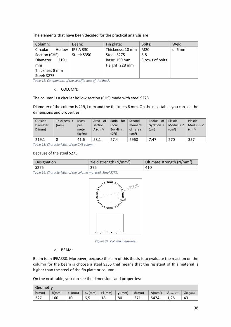
38

The elements that have been decided for the practical analysis are:

Column: Beam: Fin plate: Bolts: Weld

Circular Hollow Section (CHS) Diameter 219,1 mm Thickness 8 mm Steel: S275

IPE A 330 Steel: S350

Thickness: 10 mm Steel: S275 Base: 150 mm Height: 228 mm

M20 8.8 3 rows of bolts

e: 6 mm

Table 12: Components of the specific case of the thesis

o COLUMN:

The column is a circular hollow section (CHS) made with steel S275.

Diameter of the column is 219,1 mm and the thickness 8 mm. On the next table, you can see the

dimensions and properties:

Outside Diameter D (mm)

Thickness t (mm)

Mass per meter (kg/m)

Area of section A (cm2)

Ratio for Local Buckling (D/t)

Second moment of area I (cm4)

Radius of Gyration r (cm)

Elastic Modulus Z (cm3)

Plastic Modulus Z (cm3)

219,1 8 41,6 53,1 27,4 2960 7,47 270 357 Table 13: Characteristics of the CHS column

Because of the steel S275.

Designation Yield strength (N/mm2) Ultimate strength (N/mm2)

S275 275 410 Table 14: Characteristics of the column material. Steal S275.

Figure 34: Column measures.

o BEAM:

Beam is an IPEA330. Moreover, because the aim of this thesis is to evaluate the reaction on the

column for the beam is choose a steel S355 that means that the resistant of this material is

higher than the steel of the fin plate or column.

On the next table, you can see the dimensions and properties:

Geometry h(mm) b(mm) tf (mm) tw (mm) r1(mm) ys(mm) d(mm) A(mm2) AL(m2 m-1) G(kg/m)

327 160 10 6,5 18 80 271 5474 1,25 43

39

Section properties

Axis y Axis z Iy(mm4) Wy1(mm3) Wy,pl(mm3) Iy(mm) Sy(mm3) Iz(mm4) Wz1(mm3) Wz,pl(mm3) Iz(mm) Sz(mm3) 1,02E+8 6,26E+5 7,02E+5 136,7 3,51E+5 6,85E+6 8,56E+4 1,33E+5 35,4 6,66E+4

Table 15: Geometry characteristics of the beam of the specific case

Warping and buckling

Iw iw It ipc 1,72E+11 39,6 1,96E+5 141,2

Table 16: Warping and buckling of the beam of the case

Designation Yield strength (N/mm2) Ultimate strength (N/mm2)

S355 355 470 Table 17: Material characteristics of the beam. Steel S355

Figure 35: Beam measures with the hollow of the bolts

o Plate

h (mm) b (mm) t (mm)

228 150 10 Table 18: Fin plate dimensions

Designation Yield strength (N/mm2) Ultimate strength (N/mm2)

S275 275 410 Table 19: Material characteristics of the fin plate

Figure 36: Fin plate measures with the hollow of the bolts

40

o Bolts

6 bolts M20 with designation 8.8.

Designation Yield strength (N/mm2) Ultimate strength (N/mm2)

8.8 640 800 Table 20: Characteristics of the bolts used on the specific case

d (mm) d0 (mm)

20 22 Table 21: Characteristic of the diameters. Bolts diameter and hollow of bolt diameter

o Concrete:

The designation of the concrete is C25/30. On the Eurocode indicates that some of the relevant

values are:

fck (MPa) fcm (MPa) fctm (MPa) Ecm (GPa)

25 33 2,6 30,5 Table 22: Resistance of the concrete C25/30.

3.2 Analytical calculations As it is shown in 2.1.1 and 2.1.2 there are few calculations to anticipate how the composite

structure is going to react.

One of the aims of that thesis is the comparison of a composite and non-composite column,

because of that, the next calculations are going to be for a composite and steel cylinder tubular

column.

3.2.1 Buckling calculation One of the commons failures of a column is because of the bucking. It is obvious that the

composite structure will resist more, but, how much more load can resist a composite column

is the fact that it will be evaluate.

The next calculations are going to be theoretical calculations and for that, we must calculate by

Euler equations. Euler’s critical load defines the maximum load that a column can support before

the buckling.

𝑃𝑐𝑟 = 𝜋2 · 𝐸 · 𝐼

𝐿𝑐𝑟𝑖2

eq. 49

Where the Lcri is the critical Euler length of column.

Figure 37: Definition of Lcri of Euler

In that case is going to choose the option that both limits are: rotation fixed and translation

fixed.

41

The length of the column is decided to 3,5 meters because is a common length for that type of

elements. Other values are going to be consider following Eurocodes. [11]

3.2.1.1 Steel column For the steel column we need the properties of the section, these properties we can found it in

a catalog that includes the section of the column that we want to analyze.

Ones we have the properties of the section (I) we need the properties of the material (E) in this

case: Steel. The most common value for the young's modulus in steel is: 210.000 MPa (N/mm2).

Now we can proceed to calculate with eq. 49:

𝑃𝑐𝑟 = 𝜋2 · 210000 · 2960 · 104

(0,5 · 3500)2

𝑃𝑐𝑟 = 20.032,477 𝑘𝑁

3.2.1.2 Composite column To calculate the maximum load for the bucking of a composite column it is going to use the same

equation. The difference now is how to determinate the section and material properties.

These value is going to be absolutely theoretical because as we know to define a common value

that englobes both materials are complex. Otherwise, the simplified method defines: (eq. 10)

𝐸𝐼 = 𝐸𝑎 ∗ 𝐼𝑎 + 0,6 ∗ 𝐸𝑐𝑚 ∗ 𝐼𝑐 + 𝐸𝑠 ∗ 𝐼𝑠

As it is show in eq. 49:

𝐸𝐼 = 210000 · 2960 · 104 + 0,6 · 30500 · 8352,37 · 104

𝐸𝐼 = 77444,8371 · 108𝑁𝑚𝑚2

𝑃𝑐𝑟 = 𝜋2 · 77444,8371 · 108

(0,5 · 3500)2

𝑃𝑐𝑟 = 24958,364 𝑘𝑁

If the load is not on the center of the column exists a combination of axial and bending moment,

furthermore, as we know from the theoretical bases 2.1 Behaviour peculiarities of composite

we can study and evaluate the maximum axial and bending moment. To calculate the bucking

of the composite column we will evaluate the local bucking and searching for the interaction

curve. We want to obtain the maximum load that the joint, or in this case the column, can afford.

After developing the interaction curve, we will found a lineal rule for the case that we are

studding and see which is the maximum load that the joint can afford.

The calculations of the interaction curves and the next axial compression is based on the Design

guide 5: For concrete filled hollow sections columns under static and seismic loading.

42

Initial data:

Concrete Safety factors

fck(MPa) 25 ϒa 1,1

fcm(MPa) 33 ϒc 1,5

fctm(MPa) 2,6 ϒs 1,15

Ac (mm2) 32397,37 Column length

Ic (mm4) 83523700 L(mm) 3500

Ecm(GPa) 31

Steel column

d (mm) 219,1

t (mm) 8

fy(MPa) 275

Aa(mm2) 5310

Ia (mm4) 29600000 Table 23: Initial data to calculate the local bucking

For knowing the interaction curve, first we need to study each one of the points that it is

composed.

Squash load (eq. 6) (eq. 11):

𝑁𝑝𝑙, 𝑅𝑑 = 𝐴𝑎 · 𝑓𝑦𝑑 + 𝐴𝑐 · 𝑓𝑐𝑑 + 𝐴𝑠 · 𝑓𝑠𝑑

𝑁𝑝𝑙, 𝑅𝑑 = 5310 ·275

1,1+ 32397,37 ·

25

1,5

𝑁𝑝𝑙, 𝑅𝑑 = 1867456 𝑁 = 1876,456 𝑘𝑃𝑎

0,2 < 𝛿 < 0,9

𝛿 =𝐴𝑎 · 𝑓𝑦𝑑

𝑁𝑝𝑙, 𝑅𝑑

𝛿 =5310 ·

2751,1

1867456= 0,711

Check of local bucking (eq. 14)

Being a circular hollow section:

𝑑

𝑡< 77

219,1

8= 27,39 < 77

Axial compression

Effective stiffness (eq. 10):

(𝐸𝐼)𝑒 = 𝐸𝑎 · 𝐼𝑎 + 0,8 · 𝐸𝑐𝑑 · 𝐼𝑐 + 𝐸𝑠 · 𝐼𝑠

(𝐸𝐼)𝑒 = 63892300 · 108 𝑁/𝑚𝑚2

43

Bucking load (eq. 9):

𝑁𝑐𝑟 =(𝐸𝐼)𝑒 · 𝜋2

𝐿2

𝑁𝑐𝑟 = 5147691,051 𝑁

Relative slenderness (eq. 7):

𝜆̅ = √𝑁𝑝𝑙, 𝑅𝑑

𝑁𝑐𝑟= √

1867456

5147691,051= 0,664

Bucking curve a:

Table 24: Bucking curve. Eurocode.

𝝌 =1

𝛷 + √𝛷2 − 𝜆̅ 2

𝛷 = 0,5[1 + 0,21 · (𝜆̅ − 0,2) + 𝜆̅ 2]

𝛷 = 0,5[1 + 0,21 · (0,664 − 0,2) + 0,6642] = 0,7692

𝝌 =1

𝛷 + √𝛷2 − 𝜆̅ 2=

1

0,7692 + √0,76922 − 0,6642

𝝌 = 0,86

Check for creep and shrinkage:

𝜆̅ <0,8

1 − 𝛿=

0,8

1 − 0,711= 2,768

𝜆̅ = 0,664 < 2,768

𝑁𝑜 𝑖𝑛𝑓𝑙𝑢𝑒𝑛𝑐𝑒 𝑜𝑛 𝑡ℎ𝑒 𝑏𝑒𝑎𝑟𝑖𝑛𝑔 𝑐𝑎𝑝𝑎𝑐𝑖𝑡𝑦

Check for bearing capacity (eq. 5):

44

𝑁𝑠𝑑 ≤ 𝑁𝑅𝑑

𝑁𝑠𝑑 ≤ 𝑁𝑝𝑙, 𝑅𝑑 · 𝝌 = 1606012 N

𝑁𝑠𝑑 < 1606,012 𝑘𝑁

You must remember that load is in an axial way, without eccentricity.

Cross-section interaction curve:

Plastic section moduli:

𝑊𝑝𝑠 = 0

𝑊𝑝𝑐 =(𝑑 − 2 · 𝑡)3

6−𝑊𝑝𝑠 =

(219,1 − 2 · 8)3

6− 0

𝑊𝑝𝑐 = 1396299,299 𝑚𝑚3

𝑊𝑝𝑎 =𝑑3

6−𝑊𝑝𝑐 −𝑊𝑝𝑠 =

219,13

6− 1396299,299 − 0

𝑊𝑝𝑎 = 356676,3467 𝑚𝑚3

Interaction point D:

𝑀𝐷, 𝑅𝑑 = 𝑀𝑚𝑎𝑥, 𝑅𝑑 = 𝑊𝑝𝑎 · 𝑓𝑦𝑑 +1

2· 𝑊𝑝𝑐 · 𝑓𝑐𝑑 +𝑊𝑝𝑠 · 𝑓𝑠𝑑

𝑀𝐷,𝑅𝑑 = 356676,3467 ·275

1,1+1

2· 1396299,299 ·

25

1,5+ 0

𝑀𝐷,𝑅𝑑 = 100804917,2 𝑁𝑚𝑚

𝑁𝐷, 𝑅𝑑 =1

2· 𝑁𝑝𝑙, 𝑐, 𝑅𝑑 =

1

2· 𝐴𝑐 · 𝑓𝑐𝑑 =

1

2· 32397,37 ·

25

1,5

𝑁𝐷, 𝑅𝑑 = 269978,083 𝑁

Interaction point C and B:

𝑁𝐶, 𝑅𝑑 = 2 · 𝑁𝐷, 𝑅𝑑 = 𝑁𝑝𝑙, 𝑐, 𝑅𝑑 = 𝐴𝑐 · 𝑓𝑐𝑑

𝑁𝐶, 𝑅𝑑 = 32397,37 ·25

1,5= 539956,167

For a circular hollow section filled of concrete hn:

ℎ𝑛 =𝑁𝑝𝑙, 𝑐, 𝑅𝑑 − 𝑁𝑝𝑙, 𝑠, 𝑅𝑑

2 · 𝑑 · 𝑓𝑐𝑑 + 4 · 𝑡 · (2 · 𝑓𝑦𝑑 − 𝑓𝑐𝑑)

ℎ𝑛 = 23,713 𝑚𝑚

2 · ℎ𝑛 = 47,43 𝑚𝑚

Plastic section moduli of the cross sectional areas in the region of 2·hn

𝑊𝑝𝑠𝑛 = 0

45

𝑊𝑝𝑐𝑛 = (𝑑 − 2 · 𝑡) · ℎ𝑛2 = (219.1 − 2 · 8) · 23,7132 = 114209,143

𝑊𝑝𝑎𝑛 = 2 · 𝑡 · ℎ𝑛2 = 2 · 8 · 23,7132 = 8997,274

𝑀𝑛, 𝑅𝑑 = 𝑊𝑝𝑎𝑛 · 𝑓𝑦𝑑 +1

2· 𝑊𝑝𝑐𝑛 · 𝑓𝑐𝑑 +𝑊𝑝𝑠𝑛 · 𝑓𝑠𝑑

𝑀𝑛, 𝑅𝑑 = 8997,274 ·275

1,1+1

2· 114209,143 ·

25

1,5= 3201061,286

𝑀𝑝𝑙, 𝑅𝑑 = 𝑀𝐵, 𝑅𝑑 = 97603853 𝑁𝑚𝑚

Non-dimensional interaction curve:

NRd/Npl,Rd MRd/Mpl,Rd

A 0 1

B 1 0

C 1 0,28914

D 1,032796 0,14457

Now the question is: Which is the maximum load that the column can afford on this case?

We know that the bending moment is connected with the shear, because the bending moment

appears because of the eccentricity of the shear, so we can know with is the maximum

combination of both that the system can have before fail.

The condition that must be verify:

𝑀𝑠𝑑 = 𝑁𝑠𝑑 · 𝑒

00,05

0,10,15

0,20,25

0,30,35

0,40,45

0,50,55

0,60,65

0,70,75

0,80,85

0,90,95

11,05

0 0,2 0,4 0,6 0,8 1 1,2

NR

d/N

pl,R

d

MRd/Mpl,Rd

Non-dimensional interaction curve

Graph 1: Non-dimensional of interaction on this specific case.

46

With this expression, we can found the rule that follows:

If we mixt both graphs we can found with is the highest combination that the column can afford:

Graph 3: Interaction curve and specific case line.

Now the relevant part is analyse the point where both curves math.

0

0,2

0,4

0,6

0,8

1

1,2

0 0,2 0,4 0,6 0,8 1 1,2 1,4

NR

d/N

pl,R

d

MRd/Mpl,Rd

specificcase

interactioncurve

NSd/Npl,Rd MSd/Mpl,Rd

0 0

0,1 0,15306414

0,2 0,30612827

0,3 0,45919241

0,4 0,61225654

0,5 0,76532068

0,6 0,91838481

0,7 1,07144895

0,8 1,22451308

Table 25: specific points of graph

0

0,1

0,2

0,3

0,4

0,5

0,6

0,7

0,8

0,9

0 0,2 0,4 0,6 0,8 1 1,2 1,4

NR

d/N

pl,R

d

MRd/Mpl,Rd

Specific case relation N and M

Graph 2: Relation between NRd/Npl,Rd and MRd/Mpl,Rd on the specific case

47

Graph 4: Interaction curve and specific case graph with their lineal function

We can found that the point is defined by:

X 0,73303

Y 0,478889

𝑥 =𝑀𝑅𝑑

𝑀𝑝𝑙, 𝑅𝑑

𝑀𝑅𝑑 = 71546552,3 𝑁𝑚𝑚

𝑀𝑅𝑑 = 71,547 𝑘𝑁𝑚

𝑦 =𝑁𝑅𝑑

𝑁𝑝𝑙, 𝑅𝑑

𝑁𝑅𝑑 = 894304,216 𝑁

𝑵𝑹𝒅 = 𝟖𝟗𝟒, 𝟑𝟎𝟒 𝒌𝑵

Therefore, for the meaning of buckling, the shearing load must be higher than 894,304kN on the

beam.

y = 0,6533x - 3E-16R² = 1

y = -0,7109x + 1R² = 1

0

0,1

0,2

0,3

0,4

0,5

0,6

0,7

0,8

0,9

1

0 0,2 0,4 0,6 0,8 1 1,2 1,4

NR

d/N

pl,R

d

MRd/Mpl,Rd

specific case

first part ofinteractioncurve

Linear (specificcase)

Linear (firstpart ofinteractioncurve)

48

3.2.2 Joint calculation

3.2.2.1 Steel column For that type of connection, only made by steel, we must check Eurocode 3: Design of steel

structures.

To be a successful joint, it is necessary to be verify:

o BEAM

Shearing resistance

Bearing resistance

Block tearing

o FIN PLATE

Shearing resistance

Bearing resistance

Block tearing

o BOLT

Shearing resistance

Bearing resistance

o WELD

o COLUMN

Punching shear resistance

Supporting column wall

The lowest maximum load that is calculated in that verifications will define the maximum load

of the join and where.

o BEAM

Shearing resistance

𝑉𝑅𝑑 =

𝐴𝑣𝑧 ·𝑓𝑦

√3𝛾𝑀0

=

26,99 · 102 ·355

√31,05

= 526,843𝑘𝑁

Bearing resistance (eq. 30)

𝐹𝑏, 𝑢 =𝑘1 ·∝ 𝑏 · 𝑓𝑢 · 𝑑 · 𝑡

𝛾𝑀2

Where k1 is the minimum value:

For edge bolts:

2,8𝑒2

𝑑0− 1,7 = 2,8

35

22− 1,7 = 2,75

1,4𝑝2

𝑑0− 1,7 = 1,4

70

22− 1,7 = 2,75

𝟐, 𝟓

For inner bolts:

1,4𝑝2

𝑑0− 1,7 = 1,4

70

22− 1,7 = 2,75

49

Figure 38: Block tearing beam

𝟐, 𝟓

Where ∝b is the minimum value:

∝d

𝑓𝑢𝑏

𝑓𝑢=800

430= 1,70

1

Where ∝d is the minimum value:

End bolts:

𝑒1

3 · 𝑑𝑜=

84,5

3 · 22= 1,28

Inner bolts:

𝑝1

3 · 𝑑𝑜−1

4=

79

3 · 22−1

4= 0,947

Finally we can obtain Fv,u value:

𝐹𝑏, 𝑢 =2,5 · 0,94697 · 470 · 22 · 6,5

1,25= 127,292 𝑘𝑁

For 3 bolts:

(𝐹𝑏, 𝑢)𝑡𝑜𝑡𝑎𝑙 = 6 ∗ 𝐹𝑏, 𝑢 = 𝟕𝟔𝟑, 𝟕𝟓𝟎 𝒌𝑵

Block tearing (eq. 35)

𝑉𝑒𝑓𝑓 = 0,5 · 𝑓𝑢 ·𝐴𝑛𝑡

𝛾𝑀2+

𝐴𝑛𝑣 ·𝑓𝑦

√3𝛾𝑀0

𝑉𝑒𝑓𝑓 = 0,5 · 470 ·(35−22/2)·6,5

1,25+

(84,5+79·2−22·2−11)·6.5·355

√3

1,05

𝑉𝑒𝑓𝑓 = 𝟑𝟐𝟓, 𝟖𝟖𝟑 𝒌𝑵

o FIN PLATE

Shearing resistance

𝐹𝑣, 𝑅𝑑 =𝛼𝑣 · 𝑓𝑢 · 𝐴𝑠

𝛾𝑀2

The value of 𝛼𝑣 is 0,6 because the class of the bolt is 8.8

On Eurocode we can check the value of As. Bolt of 20 cm of

diameter have 245 mm of As.

𝐹𝑣, 𝑅𝑑 =0,6 · 800 · 245

1,25

𝐹𝑣, 𝑅𝑑 = 94,08 𝑘𝑁

Anv

Anv Ant

Ant

50

For 6 bolts that there are on every fin plate:

𝑛 · 𝐹𝑣, 𝑅𝑑 = 𝟓𝟔𝟒, 𝟒𝟖 𝒌𝑵 Bearing resistance (eq. 30)

𝐹𝑏, 𝑢 =𝑘1 ·∝ 𝑏 · 𝑓𝑢 · 𝑑 · 𝑡

𝛾𝑀2

Where k1 is the minimum value of:

For edge bolts:

2,8𝑒2

𝑑0− 1,7 = 2,8

35

22− 1,7 = 2,75

1,4𝑝2

𝑑0− 1,7 = 1,4

70

22− 1,7 = 2,75

𝟐, 𝟓

For inner bolts:

1,4𝑝2

𝑑0− 1,7 = 1,4

70

22− 1,7 = 2,75

𝟐, 𝟓

Where ∝b is the minimum value:

∝d

𝑓𝑢𝑏

𝑓𝑢=800

430= 1,70

1

Where ∝d is the minimum value:

End bolts:

𝑒1

3 · 𝑑𝑜=

35

3 · 22= 𝟎, 𝟓𝟑

Inner bolts:

𝑝1

3 · 𝑑𝑜−1

4=

79

3 · 22−1

4= 0,947

Finally we can obtain Fv,u value:

𝐹𝑏, 𝑢 =2,5 · 0,53 · 430 · 22 · 10

1,25= 95,66 𝑘𝑁

For 6 bolts:

(𝐹𝑣, 𝑢)𝑡𝑜𝑡𝑎𝑙 = 6 · 𝐹𝑣, 𝑢 = 𝟓𝟕𝟒, 𝟎𝟎 𝒌𝑵

51

Figure 39: Block tearing fin plate

Block tearing (eq. 35)

𝑉𝑒𝑓𝑓 = 0,5 · 𝑓𝑢 ·𝐴𝑛𝑡

𝛾𝑀2+

𝐴𝑛𝑣 ·𝑓𝑦

√3𝛾𝑀0

𝑉𝑒𝑓𝑓 = 0,5 · 430 ·(45 + 70 − 22 − 11) · 10

1,25+

(35 + 79 + 79 − 2 · 22 − 11) · 10 ·275

√31,05

𝑉𝑒𝑓𝑓 = 𝟑𝟒𝟑, 𝟏𝟓 𝒌𝑵

o BOLT

Shearing resistance (eq. 29)

𝐹𝑣, 𝑅𝑑 =∝ 𝑣 · 𝑓𝑢 · 𝐴

𝛾𝑀2=0,6 · 800 · 245

1,25

𝐹𝑣, 𝑅𝑑 = 94,08 𝑘𝑁 (𝐹𝑣, 𝑅𝑑)𝑡𝑜𝑡𝑎𝑙 = 𝐹𝑣, 𝑅𝑑 · 3(𝑏𝑜𝑙𝑡𝑠)

(𝐹𝑣, 𝑅𝑑)𝑡𝑜𝑡𝑎𝑙 = 564,48 𝑘𝑁

o WELD

Hypothesis: upper and lower weld are not considered.

√𝜎˔2 + 3 · (𝜏˔2 + 𝜏ǁ2) ≤𝑓𝑢

𝛽𝑤 · 𝛾𝑀𝑤 (eq. 27)

𝜏˔ = 𝜎˔

𝜏ǁ =𝐹

2 · (𝑙 · 𝑎)

𝜎˔ =1

√2· 𝜎˔ ∗ (𝜎˔ ∗=

𝑀

𝑊=𝐹 · 𝑒

2·

6

𝑎 · 𝐿2)

√(1

√2·𝐹 · 𝑒

2·

6

𝑎 · 𝐿2)2 + 3 · ((

1

√2·𝐹 · 𝑒

2·

6

𝑎 · 𝐿2)2

+ (𝐹

2 · 𝑙 · 𝑎)2

) ≤𝑓𝑢

𝛽𝑤 · 𝛾𝑀𝑤

√(1

√2·𝐹 · 80

2·

6

6 · 2282)2 + 3((

1

√2·𝐹 · 80

2·

6

6 · 228)2

+ (𝐹

2 · 228 · 6)2

) ≤430

0,85 · 1,25

If we analyse the maximum value of F to verify the expression F must be:

𝐹 < 𝟑𝟕𝟏, 𝟗𝟎𝟕 𝒌𝑵

If we evaluate the value of F:

𝐹 ≤ 659,377 𝑘𝑁

COLUMN

Punching shear resistance

𝑡𝑝 ≤ 𝑡𝑐 ·𝑓𝑢𝑐

𝑓𝑦, 𝑝

Anv

Anv Ant

Tabl

e

26:

stre

nght

clas

ses

for

con

cret

e.

(Eur

oco

de

2)An

t

Figure 40: Representation of the weld, loads and stress that affects it.

52

10 ≤ 8 ·430

275

10 ≤ 12,5

Supporting column wall (Figure 28: Example of the calculation of

column wall resistance. Eurocode 3.)

𝐹𝑅𝑑, 𝑢 =5 · 𝑓𝑦, 𝑐 · 𝑡𝑐2 · (1 + 0,25 · 𝜂) · 0,67

𝛾𝑀𝑢

Where η:

𝜂 =ℎ1

𝑑𝑐=228

219= 1,041

𝐹𝑅𝑑, 𝑢 =5 · 275 · 82 · (1 + 0,25 · 1,041) · 0,67

1,1

𝐹𝑅𝑑, 𝑢 = 67,54432 𝑘𝑁

That is the horizontal load, if we want to know the higher shear

load:

𝑀𝑓 = 𝐹𝑅𝑑, 𝑢 · ℎ

𝑀𝑓 = 𝐹 · 𝑒

𝐹 =𝐹𝑅𝑑, 𝑢 · ℎ

𝑒=67,544 · 228

80

𝐹 = 192,501

RESULTS SUMMARY:

BEAM

Shearing resistance 526,843

Bearing resistance 763,750

Block tearing 325,883

FIN PLATE

Shearing resistance 564,480

Bearing resistance 574,000

Block tearing 343,151

BOLTS Shearing resistance 564,480

WELDS Resistance 371,907

COLUMN Punching shear resistance 10≤12,5

Supporting column wall 192,501 Table 27: Results summary of steel column joint.

That join can support a maximum load of 192,501kN or before the column wall fail.

53

3.2.2.2 Composite column As we know and it was on the main topics on the theoretical part of the thesis, the calculations

of the composite columns are not a rule nowadays, so is not something that we can know how

to develop.

So in this part we will try to do some relevant calculations that we have nowadays.

How we can know why the composite joint breaks, for the beam and the bolts the criteria is the

same, we have the same beam, fin plate and bolts, so:

BEAM

Shearing resistance 336,444

Bearing resistance 308,16

Block tearing 210,176

FIN PLATE

Shearing resistance 362,905

Bearing resistance 257,94

Block tearing 318,66

BOLTS Shearing resistance 564,48

WELDS Resistance 659,377 Table 28: Some results for composite column joint.

For the column, obviously, the results and the criteria change radically.

If we try to follow the Design guide 9, we can found on the section: Connections to concrete

filled columns/ Simple shear connections/ connection design: “for the design of the connection

itself, it is generally recommended that the same criteria as given in chapter 5 (for hollow

sections without concrete filling) be used. Concrete filling of the hollow section column prevents

inward deformation of the column face, so the one column face rotational failure mode identified

in chapter 5 (for just stiffened seat connections, in section 5.9) need not be considered with

concrete filled columns. However, there is one important provision to these recommendations

relating to fire conditions.”[10]

Of course, the design guide indicate us to do the same calculations than before without

considering the column wall failure. That means that our joint will fail on:

BEAM

Shearing resistance 336,444

Bearing resistance 308,16

Block tearing 210,176

FIN PLATE

Shearing resistance 362,905

Bearing resistance 257,94

Block tearing 318,66

BOLTS Shearing resistance 564,48

WELDS Resistance 659,377 Table 29: Some results for composite column joint. Re-marking with is the failure load.

Block tearing of the beam, but what happens if we want to keep understanding on this new joint

how is the concrete and steel reaction on the column wall. Does not exist any norm that explain

it to us.

Knowing that we do not have any rule that define it we will try to do some calculations that can

orientated the joint. we decided to try to calculate with the same method that is calculated the

joints between a column and a base plate made of concrete.

54

To study how many load supports the concrete we can follow the same criteria than in a column

joint with a concrete base plate. We will calculate the design compression flange Fc,Rd:

𝐹𝑐, 𝑅𝑑 = 𝑓𝑗𝑑 ∗ 𝑏𝑒𝑓𝑓 ∗ 𝑙𝑒𝑓𝑓

𝑓𝑗𝑑 =0.6 𝑓𝑐𝑢

𝛾𝑐=0,6 ∗ 30

1,5= 12 𝑀𝑃𝑎

𝑐 = 𝑡 ∗ (𝑓𝑦

3 ∗ 𝑓𝑗𝑑 ∗ 𝛾𝑀0)0,5

= 26,97

𝐹𝑐, 𝑅𝑑 = 12 ∗ (2 ∗ 26,97 + 10) ∗ (114 ∗ 26,97)

𝐹𝑐, 𝑅𝑑 = 108,163 𝑘𝑁

𝐹 =𝐹𝑐, 𝑅𝑑 ∗ 228

𝑒= 308,265 𝑘𝑁

COLUMN column wall 308,265

Because we know that this calculations could not represent the reality we will calculate for

different fin plate thickness to compare it:

COLUMN

fin plate thickness 10 mm 308,265 kN

fin plate thickness 5 mm 138,536 kN

fin plate thickness 15 mm 506,682 kN

fin plate thickness 20 mm 734,484 kN

fin plate thickness 50 mm 2721,204 kN

55

3.3 Numerical modelling

3.3.1 Buckling modelling To calculate the critical load of the column in ANSYS it is going to do a linear buckling analysis.

ANSYS allowed doing an Eigen buckling analysis. Because of that, the column will be modeled

with their section and material properties and then a 1N force is going to be introduced on the

top.

The conditions are:

- Displacement: First and last node is going to be restricted without any

movement. These nodes cannot have a displacement or rotation, except one,

the vertical movement of the top node. That vertical axis have to be free if we

want to analyze the local buckling.

- Load: it is going to be introduce one vertical load with the value of 1 N. this

value is decided to be 1 because we can see on the solutions the critical load

directly. The solutions give to us the multiply factor, if we introduce a load

with that multiply factor the column will collapse.

3.3.1.1 Steel column For this simulation the conditions are:

Figure 42: Linear isotropic properties material. Steel column.

The results are:

That means for the first module of collapse of the column the load have to be multiply by

20037000. Because of the load have a value 1N we can know directly that for the first module

of buckling the critical load is:

Figure 43: solutions for the first 5 modes of buckling. Steel column.

Figure 41: Column representation with ANSYS APDL.

56

𝑃𝑐𝑟 = 20.037,00 𝑘𝑁

The representations of the different modules are:

1st modulus 2nd modulus 3rd modulus 4th modulus 5th modulus

Pcri=20.037,00 kN P = 41.017 kN P = 80.387 kN P = 121.980 kN P = 182.980 kN

Table 30: 5 fist modes and value of the load. Steel column.

With these representations we can see that for the 3rd, 4th and 5th it is not enough dividing the

column just in 10 elements. In that case, the only case that is relevant is the first.

3.3.1.2 Composite column That case is more complex. The global material properties of the column are not clear. We know

that the Eurocode 3 allowed defining EI as (eq. 10):

𝐸𝐼 = 𝐸𝑎 ∗ 𝐼𝑎 + 0,6 ∗ 𝐸𝑐𝑚 ∗ 𝐼𝑐 + 𝐸𝑠 ∗ 𝐼𝑠

Therefore, it is going to do the same process that in the steel column case but with different EI.

The results are:

Figure 44: First mode of bucking. Steel column.

57

Figure 45: first 5 modes of bucking. Composite column.

Figure 46: First mode of bucking. Composite column.

1st modulus 2nd modulus 3rd modulus 4th modulus 5th modulus

Pcri=24.964 kN P = 51.103 kN P = 100.150 kN P = 151.980 kN P = 227.970 kN

Figure 47: Fist modes and value of the load. Composite column

58

3.3.2 Joint modelling For the joint modelling was decided to use ANSYS workbench. It was decided to use Workbench

and not APDL because of the modelling of connections and more than one element.

On one hand, on ANSYS APDL you do not have any error, the model should be free from errors.

On the other hand, ANSYS workbench have an easier interface and the update of geometries

and boundaries too. Solve of solid and not shells are clearer.

To sum up, if you want to do an simulation to evaluate how and where is fail and see the solid

and the solutions on more than one point it is recommended to use Workbench because is more

easily done, but if you have a simple model and you want precise values of solutions is

appropriate to use ANSYS APDL.

3.3.2.1 Steel modelling Material properties about this steel is defined in Eurocode 2. Where we can found

Structural steel grade at 16 mm

Minimum yield strength at nominal thickness 16 mm

Ksi N/mm2

S275 36000 275 Table 31: Material properties S275.

Structural steel grade Tensile strength MPa at Nom thickness between 3 mm and 16 mm

S275 370-530 MPa Table 32: Material properties S275

On the case we are in a Non-lineal case, we do not want to see when the steel starts to deform

or before the plasticity, we want to evaluate the joint before the broke. That means that we will

not see just the first elastics moments of the material we will see the plasticity of the material

and that means that we need to define the material as a: Nonlinear material.

The rule that is choose to follow is: Bilinear Isotropic Hardening

The plasticity model defines the permanent deformation of the model. Exists different models

that can define the plasticity depending on the material, such as bilinear or multi-lineal. For

steel, we can suppose that the material follow a lineal rule on the elasticity deformation and

another lineal rule for the plasticity deformation.

Figure 48: Qualitative representation of a stress-strain bilinear curve

59

The reaction on the tension and compression is suppose that is equal; the yield surface is

considered Von Mises. The Von Mises yield criteria is defined by the principal stresses. [12]

The input parameters for the definition of this

method are:

𝑓𝑦 = 275 𝑀𝑃𝑎

𝐸 = 210.000𝑀𝑃𝑎

𝜈 = 0,3

With these parameters, we can draw the first part of the bilinear method. (The elastic part)

If we want to analyse the second part (plasticity part) we must introduce the inputs tangent

modulus. The tangent modulus is equivalent to the Young’s modulus, some studies defined the

tangent modulus like the 0,0001 fraction of the young’s modulus. On that case, because we want

to evaluate the plasticity like a perfect plasticity we will defined the tangent modulus like a 0

MPa.

Plastic modulus H:

H>0 Hardening Plasticity

H=0 Perfect Plasticity

H<0 Softening Plasticity

Moreover, that means that the Et=0 for the perfect plasticity.

Therefore, at final we can defined the material on the ANSYS program like:

Figure 49: Representation of Von Misses criteria

Figure 51: material properties included in ANSYS

Figure 50: Bilinear Isotropic Hardening curve

60

We can analyses that the isotropic elasticity defines the first part of the bilinear, and the bilinear

isotropic hardening defines the seconds inputs, where yield strength is the maximum stress that

the material can supported before the plasticity.

3.3.2.2 Concrete modelling On the ANSYS program, we have a material that defines properly

the concrete, Solid65. [14]

Solid65 is a material that can simulate the cracking in tension and

crushing in compression. That means that have the capacity of

different behaviour in compression and tension.

One of the restrictions for using this material is that cannot be

used on a shell model, must be a solid because the material is

represented in 3D. This material is defined by eight nodes and

three grades of freedom each one: translation in all the directions.

The most important aspect of this material is the property of

representation non-linearity of the material, can crash, crack and have plasticity deformation.

The concrete material will be defined by diferents properties on codes:

- Linear isotropic: to define poisson and young modulus ET,MATID,SOLID65 !MATERIAL SOLID65

MP,EX, MATID,30500 !EX-Elastic moduli (also EY, EZ).

MP,PRXY,MATID,0.2 !PRXY poison

- Multilinear Isotropic Hardening: to defined the stress-strain curve more acurate. It is

decided to defined like a multilinear isotropic hardening curve, now the question is

which curve we must introduce to represent the reality.

Eurocode 2 indicates which type of curve must be used depending on the simulation:

As we can see in our case we are in a structural analysis so we can use the Schematic

curve. On the same Eurocode 2 indicates the ecuation that must follow:

𝜎𝑐

𝑓𝑐𝑚=

𝑘 ∗ 𝜂 − 𝜂2

1 + (𝑘 − 2) ∗ 𝜂

eq. 50

Where 𝜂 =𝜀𝑐

𝜀𝑐1

휀𝑐1 is indicate on the Table 33: Strength classes for concrete. (Eurocode 2)

Figure 52: Solid65 material

represented in ANSYS [14]

Figure 53: 3 different types to represent stress-strain curve. Eurocode 2. [6]

61

𝑘 = 1,05 ∗ 𝐸𝑐𝑚 ∗|𝜀𝑐1|

𝑓𝑐𝑚 (fcm indicate on the Table 33: Strength classes for concrete.

(Eurocode 2))

In that case the concrete is C25 and because of that we can define the stress and strain

curve as:

Graph 5: Stress-strain of concrete C25/30. Eurocode 2.

Table 33: Strength classes for concrete. (Eurocode 2) [6]

0

5

10

15

20

25

30

35

0 0,0005 0,001 0,0015 0,002 0,0025 0,003 0,0035 0,004

Stre

ss (

MP

a)

Strain (mm/mm)

Stress-strain concretre C25/30

62

If we introduce all the curve on the ANSYS programe an error appears. The ANSYS

always calculate if the youngh modulus of the curve is the same than the ones that we

had introduce on the lineal isotropic data. Because of that the curve must be lineal on

the elastic part, considered the firts 40% of the fcm.

Because the Newton-Rapson method of calcualtion can not afford negative gradients

the first simulations have been done with just the positive gradient of the curve, and we

saw that we arribe correctly to the solution. Otherwise, just in case the program needs

valuels higher than Ɛc1 of the curve it was decided to represent as a material with a

perfect plasticity. That does not affect on the reality of the solutions. The final curve and

code to implement that properties are:

TB,MISO,MATID,1,35,0

TBTEMP,22

TBPT,,0.000433,13.2

TBPT,,0.0005,14.1636

TBPT,,0.0006,16.4997

TBPT,,0.0007,18.6741

TBPT,,0.0008,20.6885

TBPT,,0.0009,22.5442

TBPT,,0.001,24.2432

TBPT,,0.0011,25.7867

TBPT,,0.0012,27.1763

TBPT,,0.0013,28.4136

TBPT,,0.0014,29.5

TBPT,,0.0015,30.4369

TBPT,,0.0016,31.2258

TBPT,,0.0017,31.8682

TBPT,,0.0018,32.3655

TBPT,,0.0019,32.719

TBPT,,0.002,32.9301

TBPT,,0.0021,33

TBPT,,0.0022,33

TBPT,,0.0023,33

TBPT,,0.0024,33

TBPT,,0.0025,33

TBPT,,0.0026,33

Graph 7: Stress-strain curve introduced in ANSYS concrete material

0

5

10

15

20

25

30

35

0 0,0005 0,001 0,0015 0,002 0,0025 0,003 0,0035 0,004

Stre

ss (

MP

a)

Strain (mm/mm)

Stress-strain concrete C25/30

0

5

10

15

20

25

30

35

0 0,0005 0,001 0,0015 0,002 0,0025 0,003 0,0035 0,004

Stress-strain concrete C25/30

Graph 6: Stress-strain curve introduced in ANSYS concrete material.

63

- Concrete Material Data: there is the option with the material SOLID65 to introduce some

data. This data is refered to the plasticity parametres of the concrete. In this case it was

decided to use the William-Wranke Five-Parameter Criterion [13]. On the FEM program

(ANSYS) there is the option that if you include a 0 on the value of a parameter the

program will calculate with the information that it has about the material.

Each property is defined by a number and the meanings are the next ones:

Constant Meaning Value

1 Shear transfer coefficients for an open crack (βt) 0.4

2 Shear transfer coefficient for a closed crack (βc) 0.8

3 Uniaxial tensile cracking stress (fr) 2.6

4 Uniaxial crushing stress (positive) (fc) 33.3

5 Biaxial crushing stress (positive) 0

6 Ambient hydrostatic stress state for use with constants 7 and 8 0

7 Biaxial crushing stress (positive) under the ambient hydrostatic stress state (constant 6)

0

8 Uniaxial crushing stress (positive) under the ambient hydrostatic stress state (constant 6)

0

9 Stiffness multiplier for cracked tensile conditions, used if KEYOPT(7) = 1 (defaults to 0.6).

0

Table 34 : Concrete material data

The shear transfer coefficient, β, represents conditions of the crack face. The value of β

ranges from 0 to 1, with 0 representing a smooth crack (complete loos of shear transfer)

and 1 representing a rough crack (no loss of shear transfer).

The code to implement those parameters is:

TB,CONCRE, MATID,1,9

TBTEMP,0

TBDATA,1,0.4,0.8,2.6,33

Another way to write it, could be more intuitive:

TB,CONC,1,1,9, !CONCRETE PROPERTIES (NON-METAL PLASTICITY)

TBTEMP,0

TBDATA,1,0.4 !SHEAR TRANSFER COEFFICIENTS FOR AN OPEN CRACK

TBDATA,2,0.8 !SHEAR TRANSFER COEFFICIENT FOR A CLOSED CRACK

TBDATA,3,2600000 !UNIAXIAL TENSILE CRACKING STRESS

TBDATA,4,33000000 !UNIAXIAL CRUSHING STRESS

TBDATA,5,0 !BIAXIAL CRUSHING STRESS

TBDATA,6,0 !AMBIENT HYDROSTATIC STRESS STATE FOR USE WITH 7 AND 8

TBDATA,7,0 !BIAXIAL CRUSHING STRESS UNDER THE AMBIEN…

TBDATA,8,0 !UNIAXIAL CRUSHING STRESS

TBDATA,9,0 !STIFFNESS MULTIPLIER FOR CRACK TENSILE CONDITIONS

With these three codes (Linear isotropic, Multilinear isotropic and Concrete data) the concrete

will be precise enough for the static structural analysis that we want to evaluate.

3.3.2.3 Geometry The initial model is composted by more than one element:

- Beam

- Bolts

- Column

The aim of the thesis is see the connections and the answer of the column when is filled by

concrete, because of that, it was decided to simplify the model as much as we can.

Of course the entire column must be modelled and the concrete, the elements that will be

deleted are the bolts and the beam and the element that will be simplify will the fin plate.

64

We can consider that the representations is accurate because the reaction on the column will

be the same than with the beam and bolts.

Figure 54: representation of the internal loads and simplification of the real model

To represent on accurate way the reality but being simpler the final model is:

The modelling of the fin plate is the half of it. That means that the load will be located on the

point that we consider the joint.

For the representation of the contact, on this thesis, it was suppose that with a simple contact

region between the contact and the steel is enough. However, on the reality between steel and

concrete must be introduce a friction surface. Because of the complex and the time, it was

decided to represent by a simple contact at in this case and the results are accurate at all.

3.3.2.4 Finite Element Mesh The meshing is one of the most important points in a FEM analysis. Depending on the number

of elements the results are more accurate or not, but it was studied that arrives one moment

than you can include more elements that the results will be very similar but the calculations

(matrix) grows to much for the computer program. That means that is need to follow a principle

to evaluate when is enough materials for not wasting time doing analysis but having accurate

results.

Figure 55: Model of the steel and composite column with the fin plate.

65

In this case, we decided to study the same model with different size of elements and define

which one is the ones that we considered enough.

The size of the mesh is not enough when you are doing a FEM analysis; depending on the shape

of the model is need to define a number of divisions to control better the model. Furthermore,

when the model is created by a shell the meshing could be easier to control, you do not have

to control de width of the elements, when is a solid we have to be careful with the proportion

width-high it is studied that the difference between them cannot be higher than 5.

Mesh 10 mm Mesh 15 mm Mesh 25 mm

6.767 elements 2.979 elements 1.067 elements

25.337 elements 48.685 elements 4.575 elements

Figure 56: Different size of mesh in steel and composite model and the number of elements the represents.

On section of the results 3.3.2.6 Results you can found different solutions with different size of

mesh, sometimes with some restrictions.

Doing the analysis was need to do some restrictions to control the mesh and be accurate with

the solutions. Some of the restrictions are:

Figure 57: Representation of some limitations to have a precise mesh

66

To make sure that the fin plate is well defined it was decided to limit the number of elements in

the edges. 20 elements on the length and 2 elements on the width symmetry, that means 4

elements in all width plate.

3.3.2.5 Loading and Boundary Conditions The column length was evaluate too, and in some results you can find how the answer varieties

because of this fact. The general rule was to have a 1 m column, that was considered enough

accurate and comparing with the number of elements that a 3,5 meters can increase (3,5 m is

the length that columns used to have because of the floor high on a building.

Because of that, the model used to be 1 m column and the boundary conditions, that do not

variety with the different length, are fixed on the top and the bottom of the column.

To have a better image and analysis sometimes it was impose the symmetry condition.

Figure 58: Boundary conditions for the column.

Figure 59: Boundary conditions and external load. Symmetric representation.

67

3.3.2.6 Results On this section of the thesis, we will see the results that we obtain from the ANSYS program.

3.3.2.6.1 Steel joint

As we talked in the lasts points, the modelling of the steel joints is just with one material: Steel

and with the column without filled of concrete. The qualitative solutions of the joint are: fhgdg

Figure 60: Deformation qualitative pictures. ANSYS. Mesh 10 mm. View results in: 21 (0,5xAuto results).

Figure 61: Von Mises stress qualitative pictures. ANSYS. Mesh 10 mm. View results left ones in: 21 (0,5xAuto results) and right one in: 1.0 (True Scale)

68

When you are developing or studding a model by a FEM, you cannot define just with one

simulation. The solutions depends on different parameters, and because of that, must be

compared different resolutions.

a) Depending on the length of the column: one of the facts that can change the resistance

of the joint could be the length of the column, because of that, it was decided to study

the column with different sizes:

As we can see, the length of the column is not something that creates huge variations

on the results because of that it was decided to work with a 1 m column.

b) Depending on the size of mesh: always with some restrictions, talked in section 3.3.2.4

Finite Element Mesh, the size of the mesh could be different:

0

20

40

60

80

100

120

140

160

180

200

220

240

0 1 2 3 4 5 6 7 8 9 10

Load

(kN

)

Total deformation (mm)

Different length of column

0,5 m

1 m

3,5 m

0

20

40

60

80

100

120

140

160

180

200

220

240

260

280

0 1 2 3 4 5 6 7 8 9 10 11

Load

(kN

)

Total deformation (mm)

Different size of mesh

10 mm

15 mm

20 mm

Graph 8: Resolution with different length of steel column joint.

Graph 9: Resolution with different size of mesh.

69

3.3.2.6.2 Composite joint

If we evaluate the qualitative results, we can see where the joint deflects and resist more:

Figure 65: Deformation of composite column joint. ANSYS. Mesh 30 mm. View in: 21 (0,5xAuto results)

Figure 64: Von misses stress. Steel element of the composite joint. View in: 21 (0,5xAuto results)

Figure 63: Maximum principal stress. Concrete element on composite joint. View in: 21 (0,5xAuto results).

Figure 62: Minimum principal stress. Concrete element on composite joint. View in: 21 (0,5xAuto results).

70

For the steel composite column, we have more information and it was quite accurate. For

composite column, as we said on the theoretical part of the thesis the solutions are not very

sure. Because of that, we will change some parameters to see how affects the different

dimensions of the column. For example:

- Different size of mesh

- Different thickness plate:

0

50

100

150

200

250

300

350

400

450

500

550

600

0 1 2 3 4 5

Load

(kN

)

Total deformation (mm)

Composite column diferent thickness fin plate

thickness 5 mm

thickness 8 mm

thickness 10 mm

thickness 15 mm

thickness 20 mm

thickness 50 mm

Graph 10: Results for load-deformation of composite column joint. Results with different types of mesh

0

2040

6080

100

120140

160180

200

220240

260280

300

0 0,5 1 1,5 2

Load

(kN

)

Total deformation (mm)

Composite column joint

Mesh 15 mm

Mesh 20 mm

Mesh 30 mm

Graph 11: Results for load-deformation of composite column joint. Results with different fin plate thickness

71

- Different thickness of the column:

Graph 12: Results for load-deformation of composite column joint. Results with different column thickness

We can see that with different thickness of column, the failure load is very similar; the only part

that is altered is the elastic area. That is very interesting because means that the elastic area

depends on the thickness of the column, however, the plastic area is not and the joint will fail

on the same load. One of the most important conclusion that we can do in with that studies with

different thickness of the column is that the joint breaks because of the concrete.

However, the change on the thickness of the plate made the joint more resistance. With a bigger

thickness of the plate the joint will resist more. We can explain it with the less concentration of

load on the same point of the column. The load is distributed in a higher surface and that means

less stress on the column.

0

20

40

60

80

100

120

140

160

180

200

220

240

260

280

300

320

0 1 2 3 4 5 6

Loan

(kN

)

Total deformation (mm)

Results with different thickness of column

column thickness 8 mm

column thickness 12 mm

column thickness 15 mm

column thickness 30 mm

72

4 COMPARISON OF NUMERICAL MODELING AND ANALYTICAL

CALCULATIONS RESULTS The consideration of the parameters is:

- For steel joint: 10 mm mesh because is not too much elements and we can do it as

precise as we consider

- For composite joint: 15 mm mesh, we can do it with less but the time with a size of 10

mm increase to much comparing with the difference of the results. We can consider that

a mesh of 15 mm is precise.

All the columns will have a 1 m length because as we saw in steel results the solution does not

change to mush and a column of 3,5 m is many elements to evaluate.

4.1 Bucking comparison The comparison between the results are:

Analytical calculations (kN)

Numerical calculation (kN)

Error (MEF/Analytical)

BUCKING Steel column 20.032,477 20.037,00 1,0002

Composite column 24.958,364 24.964,00 1,0002 Table 35: Comparison between numerical and analytical results for both types of joints.

4.2 Joint comparison To compare the analytical and numerical solutions of the joints is not as easy as the bucking. The

bucking analysis is compare between two values; nevertheless, the joint comparison is between

a value and a graph.

The value is the calculation that we calculate that the joint will fail, and the graph is the solution

that we obtain from the ANSYS.

4.2.1 Steel column First, choose the one that we considered that will be the resolution:

020406080

100120140160180200220240

0 2 4 6 8 10 12

Load

(kN

)

Displacement (mm)

Steel joint

Table 36: Representation of the load-deformation of the steel column joint. Mesh 10 mm, length of column 1 m.

73

Now we have to consider with is the maximum load that the joint can afford. For this decision,

it is need to cross two linear rules: elastic and plastic. Study the equation that follows and

evaluate the point where they cross

LOAD 215,34kN DEFORMATION 3,22 mm

Analytical calc. Numerical calc. Error (MEF/Analytical)

Steel column 192,501kN 215,34kN 1,118

Table 38: Comparison between analytical and numerical solutions of steel column joint.

y = 65,857x + 2,9887R² = 0,9959

y = 0,6311x + 213,31R² = 0,9585

0

50

100

150

200

250

0 2 4 6 8 10 12 14

Load

(kN

)

Displacement (mm)

Steel column joint

y = 65,857x + 2,9887R² = 0,9959

y = 0,6311x + 213,31R² = 0,9585

0

50

100

150

200

250

0 2 4 6 8 10 12

Load

(kN

)

Displacement (mm)

Steel joint

Table 37: Representation of the load-deformation with the elastic and plastic linear function of the steel column joint. Mesh 10 mm, length of column 1 m.

Graph 13: Representation of the load-deformation with the elastic and plastic linear function crossing on 1 point of the steel column joint. Mesh 10 mm, length of column 1 m.

74

Furthermore, the analytical calculations are done with a security factor that the FEM (ANSYS)

does not use, so the value of the analytical calculation without the security factor is:

Supporting column wall

𝐹𝑅𝑑, 𝑢 =5 ∗ 𝑓𝑦, 𝑐 ∗ 𝑡𝑐2 ∗ (1 + 0,25 ∗ 𝜂) ∗ 0,67

𝛾𝑀𝑢

Where η:

𝜂 =ℎ1

𝑑𝑐=228

219= 1,041

𝐹𝑅𝑑, 𝑢 =5 · 275 · 82 · (1 + 0,25 · 1,041) · 0,67

1,1

𝐹𝑅𝑑, 𝑢 = 75,115 𝑘𝑁

That is the horizontal load, if we want to know the higher shear

load:

𝑀𝑓 = 𝐹𝑅𝑑, 𝑢 · ℎ

𝑀𝑓 = 𝐹 · 𝑒

𝐹 =𝐹𝑅𝑑, 𝑢 · ℎ

𝑒=75,115 · 228

80

𝐹 = 214,08 𝑘𝑁

Analytical calculations (kN)

Numerical calculation (kN)

Error (MEF/Analytical)

Error

Steel column 214,08 215,34 1,00589 1,697 % Table 39: Comparison between analytical and numerical solutions of steel column joint. Without security factor

4.2.2 Composite column The same happens than with the steel column joint, first we have to choose which is the graph

that represents better the specific case. On that moment we decided that the most accurate

results are: mesh 30 mm, 1 meter length of the column, fin plate 10 mm and thickness of the

column 8 m.

y = 328x + 9,0859R² = 0,9955

y = 1,0497x + 291,41R² = 0,9382

0

50

100

150

200

250

300

350

400

0 0,5 1 1,5 2 2,5 3 3,5 4 4,5 5

Load

(kN

)

Displacement (mm)

Composite column joint

Graph 14: Representation of the load-deformation curve for the composite column joint. Mesh 15 mm. With the plastic and elastic linear functions crossing in 1 point.

75

So, the final failure load it is considered:

LOAD 292,32 kN DEFORMATION 0,86 mm

We cannot compare with any hand value because there is any norm that told us which is the

theoretical value, but we can compare it with the value that simulates the calculation between

a steel column and a concrete plate.

Furthermore, to know if this hand calculations really works we analyses the different types of

fin plates thickness.

- 5 mm fin plate:

Graph 15: load-deformation of the composite column joint. 5 mm fin plate

LOAD 147,6369 kN DEFORMATION 0,52321 mm

y = 275,49x + 3,4979R² = 0,9961

y = 0,0132x + 147,63R² = 0,7611

0

20

40

60

80

100

120

140

160

180

0 1 2 3 4 5 6

load

(kN

)

Displacement (mm)

Composite column joint. 5 mm fin plate

Analytical calc. Numerical calc. Error (MEF/Analytical) Error

308,265 kN 292,32 kN 0,9482 5,4546 %

Analytical calc. Numerical calc. Error (MEF/Analytical) Error

139,536 kN 147,6369 kN 1,0580 5,487 %

76

- 8 mm fin plate:

LOAD 239,1714 kN DEFORMATION 0,760452 mm

In addition, we have to remember that does not affect with the column thickness, and as we

saw on the Graph 12: Results for load-deformation of composite column joint. Results with

different column thickness) the thickness of the column does not affects on the joint plasticity,

just on the elasticity and the makes that they have a similar fail load.

Analytical calc. Numerical calc. Error (MEF/Analytical) Error

237,198 kN 239,1714 kN 1,008 0,825 %

y = 301,53x + 9,8246R² = 0,99

y = 0,0313x + 239,1R² = 0,8826

0

50

100

150

200

250

300

0 1 2 3 4 5 6 7 8 9 10

load

(kN

)

Displacement(mm)

Composite column joint. 8 mm fin plate

Graph 16: load-deformation of the composite column joint. 8 mm fin plate

77

5 COMPARISON OF STEEL COLUMN AND CONCRETE COLUMN One of the most important goal of the thesis is know how the concrete column joint will react

in comparison with the steel column.

BUCKING

Maximum load (kN) Comp/Steel

Steel column 20.032,477 1,25

Composite column 24.958,364 Table 40: Bucking summary results

JOINT

Maximum load (kN) Percentage

Steel column 215,3450 35,74%

Composite column 292,3164

Deformation (mm) Percentage

Steel column 3,22 73,29%

Composite column 0,86 Table 41: Joint results summary

Table 42: Steel column joint compared to composite column joint

We can see that the composite column supports 3,22 times more than the steel column,

otherwise, the steel column is more flexible and that is sometimes an advantage.

0

30

60

90

120

150

180

210

240

270

300

330

0 2 4 6 8 10

Load

(kN

)

Displacement (mm)

Steel column vs. Composite column

composite column

steel column

78

6 CONCLUSIONS AND PROPOSALS From my point of view, there are two principal conclusions that are the most important ones:

1) On a joint with a steel tubular column, the joint will resist three times if it is filled of

concrete.

For me this is one of the most representative graphs on this thesis. One of the aim goals was

knows how the composite column on the same situation than a steel one reacts. Here we can

see that it is much more resistance, moreover, we can see that the joint is much more rigid too.

On the Design Guide, as we saw on the theoretical part of the thesis, they inform to us: “the

stiffness is about twice that of the unfilled counterparts” [10] on that case we can see that the

stiffness of the composite column is bigger than the double, it is 3,74 times stiffness than the

steel column.

Deformation (mm)

Steel column 3,22

Composite column 0,86

For the load they do not give an imposition of any load or study, just commend to us that exists confidential results on studies that are not available or have been published with insufficient information for a full interpretation, eg. the EC Composite Jacket Project, Tebbett et al.

(1979 and 1982). [10]. One of the recommendations nowadays is: have the beam less resistance than the joint and you can control your joint.

0

30

60

90

120

150

180

210

240

270

300

330

0 2 4 6 8 10

Load

(kN

)

Displacement (mm)

Steel column vs. Composite column

composite column

steel column

Graph 17: steel column vs. composite column.

79

2) Could be possible that the composite column follows the same rule that the steel

columns joint on a concrete plate. We can found the regulation in Eurocode 3 to

calculate: “6.2.5 Equivalent T-stub in compression.”

Of course for being sure that is true it must need an experimental analysis and more data.

Otherwise could be a first calculation to have an orientation of how the maximum load will be.

Analytical calc. Numerical calc. Error (MEF/Analytical)

Error

5 mm fin plate 139,536 kN 147,6369 kN 1,0580 5,487 % 8 mm fin plate 237,198 kN 239,1714 kN 1,008 0,825 % 10 mm fin plate 308,265 kN 292,32 kN 0,9482 5,4546 %

0

30

60

90

120

150

180

210

240

270

300

330

0 2 4 6 8 10

Load

(kN

)

Displacement (mm)

Composite column joint with different finplate thickness

thickness 5 mm

thickness 10 mm

thickness 8 mm

Graph 18: Composite column joint with different fin plate thickness

80

7 REFERENCES [1] Eurocode No. 4: Design of composite steel and concrete structures, Part 1: General Rules and

Rules for Buildings, ENV 1994-1-1: 1995

[2] Eggemann, H.,2006. Simplified Design of Composite Columns, Based on a Comparative Study of the Development of Building Regulations in Germany and the United States. In Proceedigns of the Second International Congress on Construction History, ed. M.Dunkeld, J. Campbell, H. Louw, M. Tutton, W. Addis & R. Thorne, vol. I, pp. 1023-1025.

[3] A. Šapalas: Behaviour, Design and Applications of composites steel – concrete structures in Lithuania. Vilnius Gediminas Technical University, Department of steel and timber structures.

[4] Y. C. Wang: Design Guide for Concrete Filled Hot Finished Structural Hollow Section (SHS) Columns, 2014

[5] g.Hanswill, Univ.-Prof. Dr. –Ing. Institute for Steel and Composite Structures. University of Wuppertal-Germany. Eurocodes Background and Applications Dissemination of information for training 18-20 February 2008, Brussels.

[6] Eurocode No. 2: Design of Concrete Structures, Part 1: General Rules and Rules for Buildings.

[7] Ronal,J.,Würker, K.-G., Dutta, D., Wardenier, J.Yeomans, N.: Structural stability of hollow sections, CIDECT series “Construction with hollow steel sections”, ISBN 3-8249-0075-0, Verlag TÜV Rheinland, Köln,1992

[8] Eurocode No. 3: Design of Steel Structures, Part 1.1: General Rules and Rules for Buildings, ENV 1993-1-1: 1992.

[9] CIDECT Monograph No. 5: For concrete filled hollow section columns under static and seismic loading. R.Bergmann, C. Matsui, C.Meinsma, D.Dutta. Verlag TÜV Rheinland, 1995

[10] CIDECT Monograph No. 9: For structural hollow section column connection. Y. Kurobane, J.A. Packer, J. Wardenier, N. Yeomans. TÜV-Verlag, 2004.

[11] Rui Simões: Eurocodes Background and Application, Design of steel building with worked examples. 16-17 October 2014, Brussels, Belgium. Department of civil engineering university of Coimbra.

[12] R.A.C. Slater, Engineering Plasticity, Theory and Application to Metal Forming Processes. 1977.

[13] Wai-Fah Chen: Plasticity in Reinforced Concrete. 1936.

[14] ANSYS, Inc. ANSYS Documentation.