HEVC Deblocking Filter

By

Arpita Dhirenkumar Yagnik

Harsha Nagathihalli Jagadish

Rohith Reddy Etikala

Acronyms

AVC: Advanced Video Coding

BS: Boundary Strength

CODEC: COder/DECoder

Croma: Chrominance

CTU: Coding Tree Unit

CU: Coding Unit

DCT: Discrete Cosine Transform

DFT: Discrete Fourier Transform

HEVC: High Efficiency Video Coding

ITU-T: International Telecommunication Union (Telecommunication Standardization Sector)

IEC: International Electrotechnical Commission

ISO: International Standards Organization

JBIG: Joint Bi-level Image Experts Group

JPEG: Joint photographic experts group

JCT-VC: Joint collaborative team on video coding

LOT: Lapped Orthogonal Transform

Luma: Luminance

MB: Macro Block

MPEG: Moving picture experts group

OBMC: Overlapped Block Motion Compensation

PU: Prediction Unit

QP: Quantization Parameter

SAO: Sample Adaptive Offset

TU: Transform Unit

1. Introduction to Blocking Artifacts

Block based transform coding is used video compression standards such as JPEG, MPEG and H.26x because it has high energy compaction and low hardware complexity. These standards achieve good compression ratio and quality of the reconstructed image and video when the quantizer is not very coarse. But, in a very low bit rate scenario, an annoying artifact in the image, called blocking artifact occurs in image and video and degrade the quality seriously. Blocking artifacts result from coarse quantization that discards most of the high frequency components of each segmented block of the original image and video and introduces severe quantization noise to the low frequency component. One example is shown in Fig. 1 to illustrate this.

Fig. 1 The highly compressed image block [2].

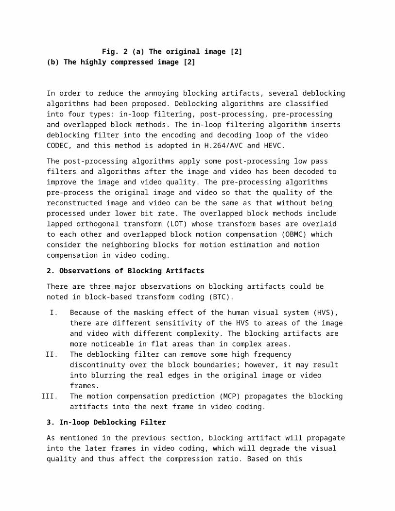
The blocking artifact incurs discontinuity across the block boundaries in the reconstructed image and video. Fig 2 (a) and (b) shows original image and compressed image, respectively. As can be seen from Fig. 2, there are many square blocks in the highly compressed image.

DCT – Discrete Cosine Transform

IDCT – Inverse Discrete Cosine Transform

Q/Q-1 – Quantization/Inverse Quantization

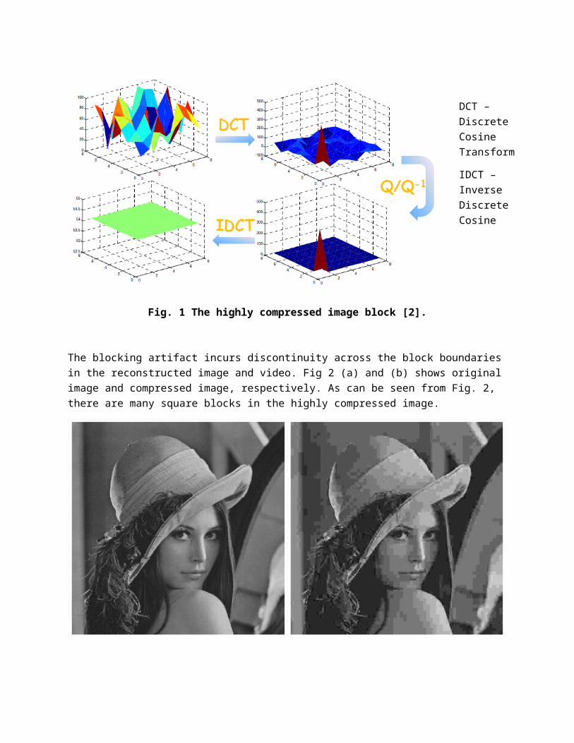
Fig. 2 (a) The original image [2] (b) The highly compressed image [2]

In order to reduce the annoying blocking artifacts, several deblocking algorithms had been proposed. Deblocking algorithms are classified into four types: in-loop filtering, post-processing, pre-processing and overlapped block methods. The in-loop filtering algorithm inserts deblocking filter into the encoding and decoding loop of the video CODEC, and this method is adopted in H.264/AVC and HEVC.

The post-processing algorithms apply some post-processing low pass filters and algorithms after the image and video has been decoded to improve the image and video quality. The pre-processing algorithms pre-process the original image and video so that the quality of the reconstructed image and video can be the same as that without being processed under lower bit rate. The overlapped block methods include lapped orthogonal transform (LOT) whose transform bases are overlaid to each other and overlapped block motion compensation (OBMC) which consider the neighboring blocks for motion estimation and motion compensation in video coding.

2. Observations of Blocking Artifacts

There are three major observations on blocking artifacts could be noted in block-based transform coding (BTC).

I. Because of the masking effect of the human visual system (HVS), there are different sensitivity of the HVS to areas of the image and video with different complexity. The blocking artifacts are more noticeable in flat areas than in complex areas.

II. The deblocking filter can remove some high frequency discontinuity over the block boundaries; however, it may result into blurring the real edges in the original image or video frames.

III. The motion compensation prediction (MCP) propagates the blocking artifacts into the next frame in video coding.

3. In-loop Deblocking Filter

As mentioned in the previous section, blocking artifact will propagate into the later frames in video coding, which will degrade the visual quality and thus affect the compression ratio. Based on this observation, higher compression ratio and better visual quality can be achieved by effectively eliminating the blocking artifacts. Therefore, HEVC, H.264/AVC and H.263+ [4], [6] add the deblocking filter into the coding loop to improve the visual quality and the accuracy of MCP.

4. H.264/AVC In-loop Deblocking Filter

In order to enhance the visual quality and coding performance, H.264/AVC adopts the in-loop filter in its coding loop. Fig. 4-1 shows the encoding architecture of H.264/AVC. As can be seen from the figure, the previously reconstructed frame passes the loop filter before motion estimation. Because the filtered frame is more similar to the original frame, obtain motion vectors can be obtained with higher accuracy.

Fig. 4-1 The encoder architecture of H.264/AVC [2].

Fig. 4-2 shows the model of two dequantized blocks across the boundaries in H.264/AVC. p0, p1, p2 and p3 denote the pixels in the left (top) 4x4 block while q0, q1, q2 and q3 denote the pixels in the right (down) 4x4 block. Because only low frequency components are reserved after coarse quantization, the discontinuity, which seems to be a newly high frequency component, comes into existence across the block boundary. Therefore, we must apply the lowpass filter to discard the new high frequency components. The orange curve indicates the pixels after filtering.

Fig. 4-2 The model of blocking artifact across the block boundary in H.264/AVC [2].

Because there are inter-frame and intra-frame coding in video compression, H.264/AVC apply the filters with different strength based on the type of coding frames. Thus, H.264/AVC encoder must determine the boundary strength (BS) before filtering. The BS parameters are determined according to Table 4-1.

Table 4-1 The coding mode based decision for the parameter BS [2].

On the other hand, H.264/AVC defines two parameters α and β to determine what type of the filter will be applied.

5. HEVC Deblocking Filter

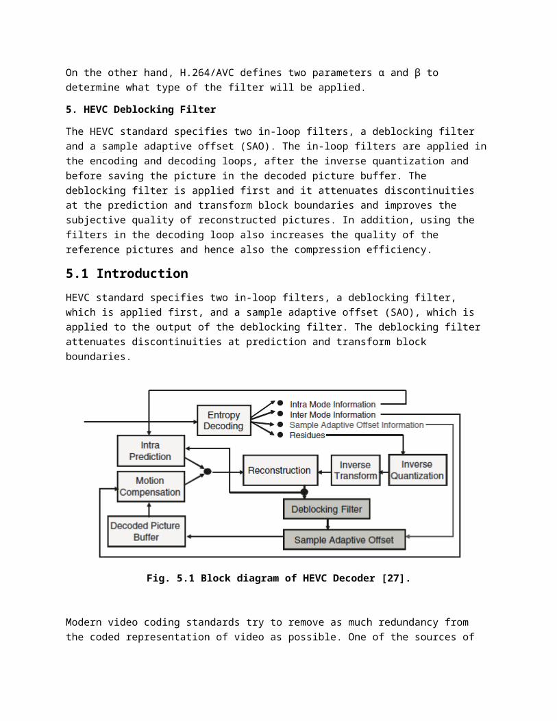
The HEVC standard specifies two in-loop filters, a deblocking filter and a sample adaptive offset (SAO). The in-loop filters are applied in the encoding and decoding loops, after the inverse quantization and before saving the picture in the decoded picture buffer. The deblocking filter is applied first and it

attenuates discontinuities at the prediction and transform block boundaries and improves the subjective quality of reconstructed pictures. In addition, using the filters in the decoding loop also increases the quality of the reference pictures and hence also the compression efficiency.

5.1 Introduction

HEVC standard specifies two in-loop filters, a deblocking filter, which is applied first, and a sample adaptive offset (SAO), which is applied to the output of the deblocking filter. The deblocking filter attenuates discontinuities at prediction and transform block boundaries.

Fig. 5.1 Block diagram of HEVC Decoder [27].

Modern video coding standards try to remove as much redundancy from the coded representation of video as possible. One of the sources of redundancy is the temporal redundancy, i.e. similarity between the subsequent pictures in a video sequence. This type of redundancy is effectively removed by motion prediction. Another type of redundancy is spatial redundancy and is removed by intra prediction from the neighboring samples and spatial transforms. In HEVC, both the motion prediction and transform coding are block-based. The size of motion predicted blocks varies from 8x4 and 4x8, to 64x64 luma samples, while the size of block transforms and intra-predicted blocks varies from 4x4 to 32x32 samples.

These blocks are coded relatively independently from the neighboring blocks and approximate the original signal with some degree of similarity. Since coded blocks only approximate the original signal, the difference between the approximations may cause discontinuities at the prediction and transform block boundaries. These discontinuities are attenuated by the deblocking filter.

There are several reasons for making in-loop filters a part of the standard. In principle, the in-loop filters can also be applied as post-filters. An advantage of using post-filters is that decoder manufacturers can create post-filters that better suit their needs. However, if the filter is a part of the standard, the encoder has control over the filter and can assure the necessary level of quality by instructing the decoder to enable the filter and specifying the filter parameters. Moreover, since the in-loop filters

increase the quality of the reference pictures, they also improve the compression efficiency. A post-filter would also require an additional buffer for filtered pictures, while the output of an in-loop filter can be kept in the decoded picture buffer (DPB). There is also another specific advantage of using the deblocking filter as an in-loop filter compared to the deblocking post-filter. If the deblocking is applied as a post-filter, block artifacts can be copied by motion estimation inside the blocks, which can make the artifacts detection more difficult and increases the deblocking complexity compared to the in-loop filtering, which needs to be applied only to the block boundaries.

It is known that the deblocking in-loop filter in H.264/AVC constitutes a significant part of the decoder complexity. Therefore, when designing the in-loop filters in HEVC, efforts have been spent on reducing the loop filters complexity, while still achieving improvements of subjective quality. The HEVC in-loop filters are easily parallelizable, which can bring advantages when running the HEVC decoders and encoders on multi-core architectures.

5.2 Block Artifacts in Video Coding

As mentioned in Sect. 5.1, in HEVC both the motion prediction and transform coding are block-based. The size of motion predicted blocks varies from 4x8 and 8x4 to 64x64 luma samples, while the size of block transforms and intra-predicted blocks varies from 4x4 to 32x32 samples. These blocks are coded relatively independently from their neighboring blocks and approximate the original signal with some degree of similarity. Since coded blocks only approximate the original signal, the difference between the approximations may cause discontinuities at the prediction and transform block boundaries. For example, motion prediction of the adjacent blocks may come from the non-adjacent areas of a reference picture (see Fig. 5.2) or even from different reference pictures. In case of non-overlapping block transforms,

Fig. 5.2 Block artifact may be created when adjacent blocks are predicted from non-adjacent areas in the reference picture [27].

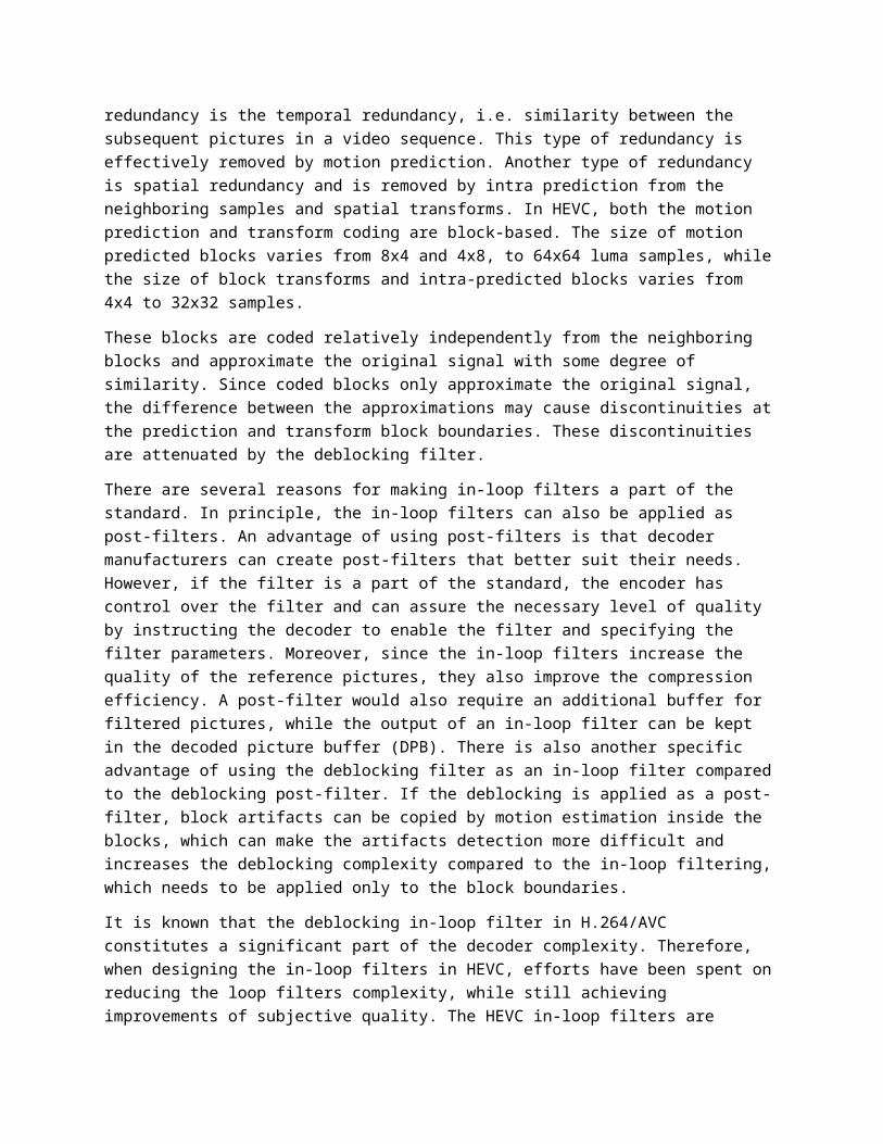
Fig 5.3 Example of block artifact in one dimension[27].

used in HEVC, coarse quantization can also create discontinuities at the block boundaries. In highly detailed areas with high-frequency content, such artifacts can be masked by the human visual system. However, in the smooth areas, discontinuities between the blocks are easily noticed by a viewer and may cause significant degradation of the perceived video quality. The example of a block artifact in one dimension is shown in Fig. 5.3. The horizontal axis shows the sample positions along a horizontal or vertical 1-D line, and the vertical axis shows the sample values.

Deblocking filter attenuates the artifacts in the areas, where they are mostly visible, i.e. in the smooth, uniform areas. The excessive filtering in the highly detailed areas should be avoided since it can cause undesirable blurring. The artifacts in those areas are rarely noticed by the human eye, while it is also more difficult to determine whether the discontinuity is caused by a block boundary or belongs to the original signal. Therefore, an important part of the deblocking filter is the deblocking filtering decisions, which determine whether a particular part of a block boundary is to be filtered. In these decisions, the HEVC deblocking filter uses the mode and motion information from the decoded bitstream as well as analyses the values of reconstructed samples on the sides of the block boundary. The strength of the deblocking filter can also be adjusted by the encoder on the picture and the slice basis.

5.3 HEVC Deblocking Filter Description

5.3.1 Decisions to Filter a Block Boundary

As a compromise between the subjective quality and computational complexity, the HEVC deblocking filter in case of 4:2:0 chroma subsampling is only applied to the block boundaries that lie at the luma and chroma sample positions that are multiples of eight (in H.264/AVC the deblocking is applied on the 4x4 luma and chroma sample grid). Since the deblocking filtering is only applied to the boundaries between the coding units (CU), prediction units (PU), or transform units (TU) and not to the inside areas,

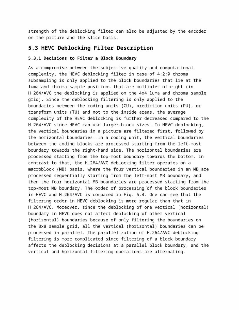
the average complexity of the HEVC deblocking is further decreased compared to the H.264/AVC since HEVC can use larger block sizes. In HEVC deblocking, the vertical boundaries in a picture are filtered first, followed by the horizontal boundaries. In a coding unit, the vertical boundaries between the coding blocks are processed starting from the left-most boundary towards the right-hand side. The horizontal boundaries are processed starting from the top-most boundary towards the bottom. In contrast to that, the H.264/AVC deblocking filter operates on a macroblock (MB) basis, where the four vertical boundaries in an MB are processed sequentially starting from the left-most MB boundary, and then the four horizontal MB boundaries are processed starting from the top-most MB boundary. The order of processing of the block boundaries in HEVC and H.264/AVC is compared in Fig. 5.4. One can see that the filtering order in HEVC deblocking is more regular than that in H.264/AVC. Moreover, since the deblocking of one vertical (horizontal) boundary in HEVC does not affect deblocking of other vertical (horizontal) boundaries because of only filtering the boundaries on the 8x8 sample grid, all the vertical (horizontal) boundaries can be processed in parallel. The parallelization of H.264/AVC deblocking filtering is more complicated since filtering of a block boundary affects the deblocking decisions at a parallel block boundary, and the vertical and horizontal filtering operations are alternating.

Fig. 5.4 Order of boundaries processing in HEVC and H.264/AVC deblocking. In each group (first to fourth), boundaries are processed from left to right and from top to bottom. In HEVC all vertical

(horizontal) boundaries can be processed in parallel [27].

A decision whether to filter a block boundary uses the bitstream information such as prediction modes and motion vectors. Some coding conditions are more likely to create strong block artifacts, which are represented by a so-called boundary strength (BS) variable that is assigned to every block boundary and is determined as in Table 5.1. The deblocking is only applied to the block boundaries with Bs greater than zero for a luma component and BS greater than 1 for chroma components. Higher values of Bs enable stronger filtering by using higher clipping parameter values. The Bs derivation conditions reflect the probability that the strongest block artifacts appear at the intra-predicted block boundaries. The conditions also enable luma deblocking when there is possibility of block artifacts caused by quantization and by prediction from non-adjacent areas in a reference picture. Not filtering block boundaries with Bs equal to zero avoids multiple repetitive filtering of static areas where the samples are just copied from one picture to another. In chroma deblocking, only the block boundaries adjacent

to intra-predicted blocks are filtered, which reduces the deblocking complexity while still removing the strongest block artifacts. The algorithm for BS derivation is explained in a flowchart in Fig. 5.5.

Table 5.1 Boundary Strength (BS) derivation [27].

Fig. 5.5 Derivation of boundary strength (BS) for block boundary. P denotes the left (or top) block and Q denotes the right (or bottom) block at the block boundary [27].

For luma block boundaries with non-zero BS values, the signal on the sides of the block boundary is evaluated to decide whether the deblocking should be applied. For chroma block boundaries, no further evaluation is performed.

BS

BS=222

BS=1 BS=0

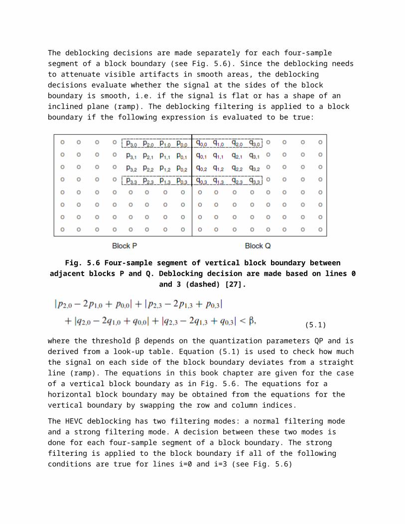
The deblocking decisions are made separately for each four-sample segment of a block boundary (see Fig. 5.6). Since the deblocking needs to attenuate visible artifacts in smooth areas, the deblocking decisions evaluate whether the signal at the sides of the block boundary is smooth, i.e. if the signal is flat or has a shape of an inclined plane (ramp). The deblocking filtering is applied to a block boundary if the following expression is evaluated to be true:

Fig. 5.6 Four-sample segment of vertical block boundary between adjacent blocks P and Q. Deblocking decision are made based on lines 0 and 3 (dashed) [27].

(5.1)

where the threshold β depends on the quantization parameters QP and is derived from a look-up table. Equation (5.1) is used to check how much the signal on each side of the block boundary deviates from a straight line (ramp). The equations in this book chapter are given for the case of a vertical block boundary as in Fig. 5.6. The equations for a horizontal block boundary may be obtained from the equations for the vertical boundary by swapping the row and column indices.

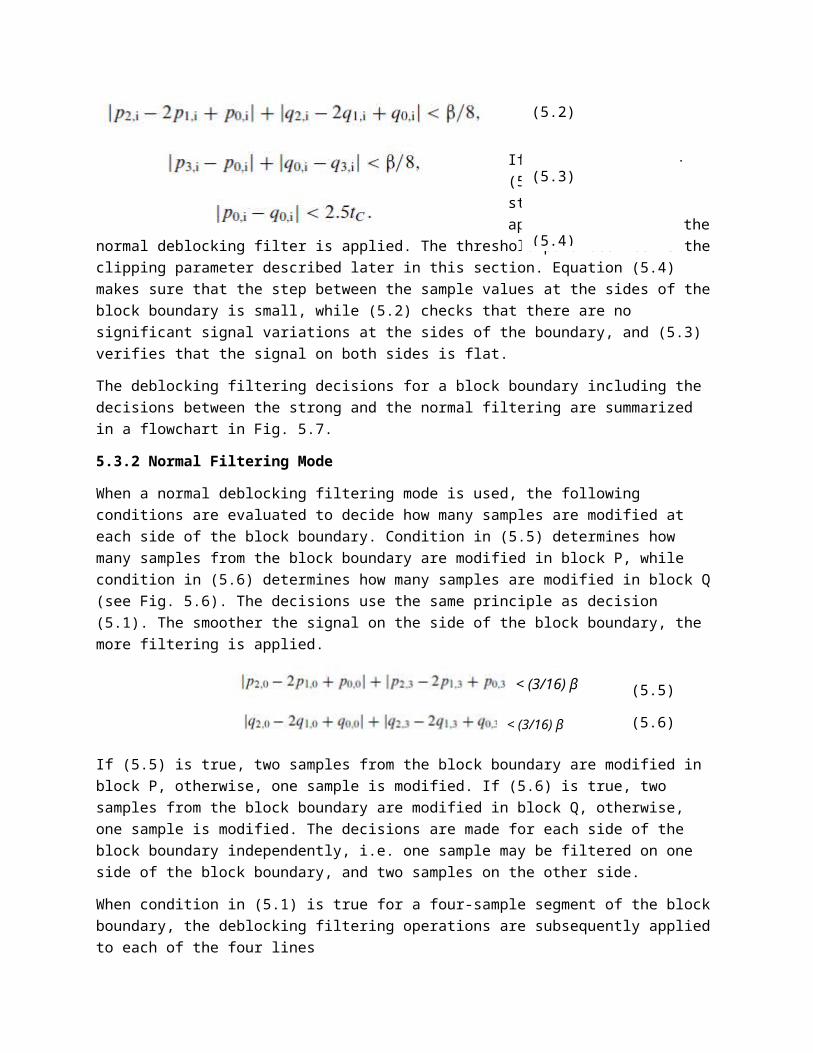
The HEVC deblocking has two filtering modes: a normal filtering mode and a strong filtering mode. A decision between these two modes is done for each four-sample segment of a block boundary. The strong filtering is applied to the block boundary if all of the following conditions are true for lines i=0 and i=3 (see Fig. 5.6)

(5.2)

(5.3)

(5.4)

If all of the (5.2)–(5.4) are true, the strong filtering is applied, otherwise, the normal deblocking filter is applied. The threshold parameter tC is the clipping parameter described later in this section. Equation (5.4) makes sure that the step between the sample values at the sides of the block boundary is small, while (5.2) checks that there are no significant signal variations at the sides of the boundary, and (5.3) verifies that the signal on both sides is flat.

The deblocking filtering decisions for a block boundary including the decisions between the strong and the normal filtering are summarized in a flowchart in Fig. 5.7.

5.3.2 Normal Filtering Mode

When a normal deblocking filtering mode is used, the following conditions are evaluated to decide how many samples are modified at each side of the block boundary. Condition in (5.5) determines how many samples from the block boundary are modified in block P, while condition in (5.6) determines how many samples are modified in block Q (see Fig. 5.6). The decisions use the same principle as decision (5.1). The smoother the signal on the side of the block boundary, the more filtering is applied.

If (5.5) is true, two samples from the block boundary are modified in block P, otherwise, one sample is modified. If (5.6) is true, two samples from the block boundary are modified in block Q, otherwise, one sample is modified. The decisions are made for each side of the block boundary independently, i.e. one sample may be filtered on one side of the block boundary, and two samples on the other side.

When condition in (5.1) is true for a four-sample segment of the block boundary, the deblocking filtering operations are subsequently applied to each of the four lines

(5.5)

(5.6)< (3/16) β

< (3/16) β

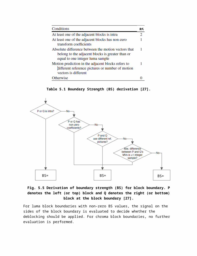
Fig. 5.7 Decisions for each four-sample segment of block boundary. PU prediction unit, TU transform unit [27].

crossing the block boundary. Since condition in (5.1) is evaluated true for the signal that forms a perfect ramp passing across the block boundary (such as a gradual change in the luma component), the deblocking in the normal filtering mode is designed to not modify the ramp. The filtered sample values p0’ and q0’ (the row index j is omitted for brevity) are determined by adding or subtracting an offset value Δ0 to each of the sample values:

where the value of Δ0 is obtained as in

(5.7)

(5.8)

where tC is a clipping parameter dependent on the QP, and Clip3(a, b, x) function clips the variable x to the range (a, b), i.e.

and δ is determined as

Neglecting the clipping operation, the impulse response of the filter is (3, 7, 9, -3)/16. The value of δ is proportional to the deviation of the signal at the sides of the block boundary from a ramp and is equal to zero when the signal across the boundary has the form of a perfect ramp across the block boundary.

Deblocking filtering is only applied to a line of samples across the block boundary if the absolute value of δ is below tC, i.e.

Expression (5.12) evaluates whether the discontinuity at the block boundary is likely to be a natural edge or caused by a block artifact.

If two samples are modified in block P, i.e. condition in (5.5) is true, the sample p1 is modified as

and if condition in (5.6) is true, sample q1 is modified as

where the p1’ and q1’ are new values of samples p1 and q1 respectively, and the values of Δ p1 and Δ q1 are obtained as follows:

The impulse response of the filter is (8, 19, –1, 9, –3)/32 if the clipping operation is neglected. One can see that the value of the offset obtained in (5.9) is used in calculation of Δp1 and Δq1. The filtering operations at positions p0, p1, q0, and q1 do not modify the signal that has a form of a perfect ramp across the block boundary.

The deblocking filter decisions done for each line of a four-sample segment of a block boundary are summarized in a flowchart in Fig. 5.8.

(5.9)

(5.10)

(5.11)

(5.12)

(5.13)

(5.14)

(5.15)

(5.16)

An example of modifications to the block boundary samples in the normal filtering mode is shown in Fig. 5.9.

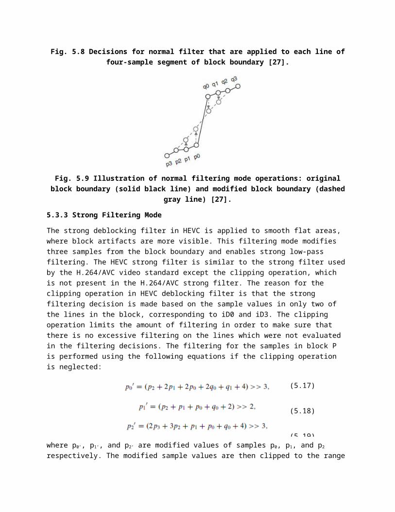
Fig. 5.8 Decisions for normal filter that are applied to each line of four-sample segment of block boundary [27].

Fig. 5.9 Illustration of normal filtering mode operations: original block boundary (solid black line) and modified block boundary (dashed gray line) [27].

5.3.3 Strong Filtering Mode

The strong deblocking filter in HEVC is applied to smooth flat areas, where block artifacts are more visible. This filtering mode modifies three samples from the block boundary and enables strong low-pass filtering. The HEVC strong filter is similar to the strong filter used by the H.264/AVC video standard except the clipping operation, which is not present in the H.264/AVC strong filter. The reason for the clipping operation in HEVC deblocking filter is that the strong filtering decision is made based on the sample values in only two of the lines in the block, corresponding to iD0 and iD3. The clipping operation limits the amount of filtering in order to make sure that there is no excessive filtering on the lines which were not evaluated in the filtering decisions. The filtering for the samples in block P is performed using the following equations if the clipping operation is neglected:

where p0’, p1’, and p2’ are modified values of samples p0, p1, and p2 respectively. The modified sample values are then clipped to the range [pi -2tC, pi +2tC]. The equations for modification of samples q0, q1, and q2 can be obtained by replacing p with q in (7.17)–(7.19).

5.3.4 Chroma Deblocking

As mentioned in Sect. 5.3.1, the deblocking is only applied to the chroma block boundaries which have boundary strength BS equal to 2, i.e. when one of the adjacent blocks is intra-predicted. The block boundary should also be a CU, TU or a prediction partition boundary and be aligned with the 8x8 chroma sample grid. No further evaluation on the signal is done for chroma block boundaries. Chroma deblocking only modifies one sample from each side of the block boundary. The following expression is used to obtain the modification offset for the chroma block boundary.

The value of Δc is used for modification of the chroma samples p0 and q0 similarly to luma samples as in (5.7) and (5.8).

(5.17)

(5.18)

(5.19)

(5.20)

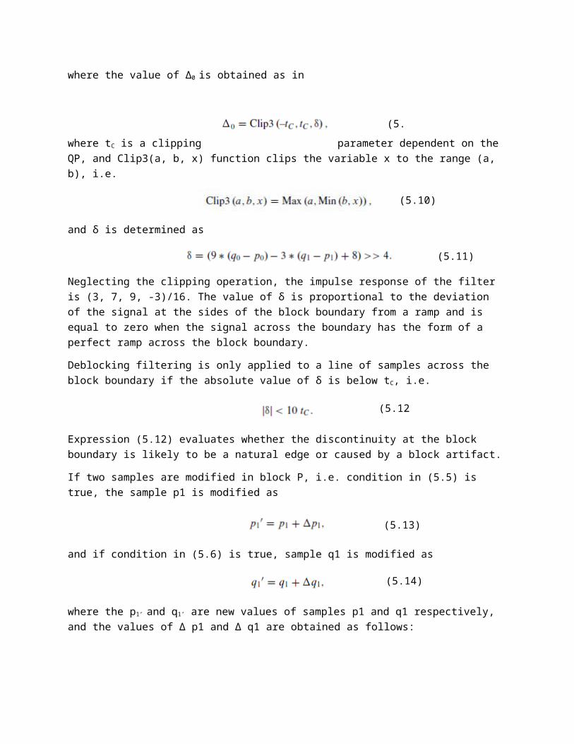
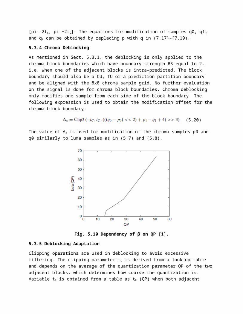
Fig. 5.10 Dependency of β on QP [1].

5.3.5 Deblocking Adaptation

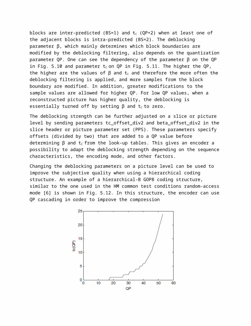
Clipping operations are used in deblocking to avoid excessive filtering. The clipping parameter tC is derived from a look-up table and depends on the average of the quantization parameter QP of the two adjacent blocks, which determines how coarse the quantization is. Variable tC is obtained from a table as tC (QP) when both adjacent blocks are inter-predicted (BS=1) and tC (QP+2) when at least one of the adjacent blocks is intra-predicted (BS=2). The deblocking parameter β, which mainly determines which block boundaries are modified by the deblocking filtering, also depends on the quantization parameter QP. One can see the dependency of the parameter β on the QP in Fig. 5.10 and parameter tC on QP in Fig. 5.11. The higher the QP, the higher are the values of β and tC and therefore the more often the deblocking filtering is applied, and more samples from the block boundary are modified. In addition, greater modifications to the sample values are allowed for higher QP. For low QP values, when a reconstructed picture has higher quality, the deblocking is essentially turned off by setting β and tC to zero.

The deblocking strength can be further adjusted on a slice or picture level by sending parameters tc_offset_div2 and beta_offset_div2 in the slice header or picture parameter set (PPS). These parameters specify offsets (divided by two) that are added to a QP value before determining β and tC

from the look-up tables. This gives an encoder a possibility to adapt the deblocking strength depending on the sequence characteristics, the encoding mode, and other factors.

Changing the deblocking parameters on a picture level can be used to improve the subjective quality when using a hierarchical coding structure. An example of a hierarchical-B GOP8 coding structure, similar to the one used in the HM common test conditions random-access mode [6] is shown in Fig. 5.12. In this structure, the encoder can use QP cascading in order to improve the compression

Fig. 5.11 Dependency of tC on QP [1].

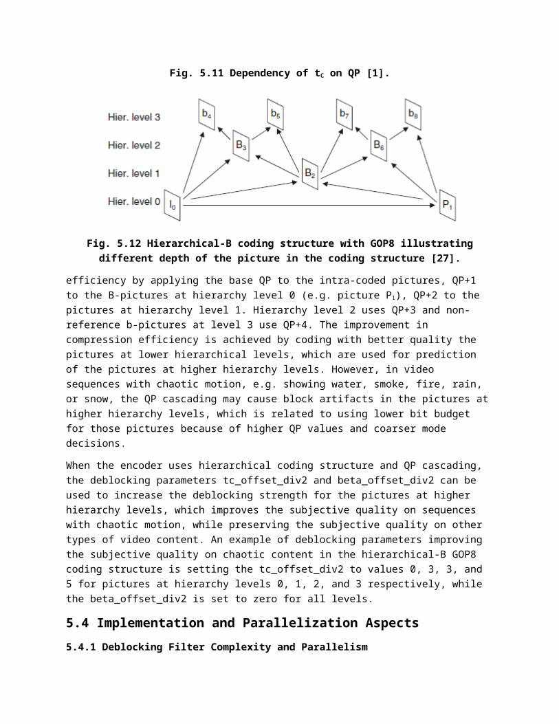
Fig. 5.12 Hierarchical-B coding structure with GOP8 illustrating different depth of the picture in the coding structure [27].

efficiency by applying the base QP to the intra-coded pictures, QP+1 to the B-pictures at hierarchy level 0 (e.g. picture P1), QP+2 to the pictures at hierarchy level 1. Hierarchy level 2 uses QP+3 and non-reference b-pictures at level 3 use QP+4. The improvement in compression efficiency is achieved by coding with better quality the pictures at lower hierarchical levels, which are used for prediction of the pictures at higher hierarchy levels. However, in video sequences with chaotic motion, e.g. showing water, smoke, fire, rain, or snow, the QP cascading may cause block artifacts in the pictures at higher hierarchy levels, which is related to using lower bit budget for those pictures because of higher QP values and coarser mode decisions.

When the encoder uses hierarchical coding structure and QP cascading, the deblocking parameters tc_offset_div2 and beta_offset_div2 can be used to increase the deblocking strength for the pictures at higher hierarchy levels, which improves the subjective quality on sequences with chaotic motion, while preserving the subjective quality on other types of video content. An example of deblocking parameters improving the subjective quality on chaotic content in the hierarchical-B GOP8 coding structure is setting

the tc_offset_div2 to values 0, 3, 3, and 5 for pictures at hierarchy levels 0, 1, 2, and 3 respectively, while the beta_offset_div2 is set to zero for all levels.

5.4 Implementation and Parallelization Aspects

5.4.1 Deblocking Filter Complexity and Parallelism

When designing the HEVC deblocking filter, a lot of attention was paid to complexity and parallelization aspects. In H.264/AVC video decoders, deblocking takes a significant part of the computational complexity. Moreover, in H.264/AVC, the deblocking operations at one block boundary may affect the samples used in deblocking of the next block boundary, which complicates parallel processing.

5.4.1.1 HEVC Deblocking Filter Complexity

The complexity of the HEVC deblocking filter has been significantly decreased compared to the H.264/AVC deblocking. First of all, the deblocking is only applied to the block boundaries on the 8x8 luma sample grid. This already decreases the worst-case complexity of the deblocking compared to H.264/AVC, where the deblocking is applied on the 4x4 sample grid. The average complexity of the deblocking operation is also decreased compared to H.264/AVC since the prediction and transform blocks in HEVC are on average larger than those in H.264/AVC, where the maximum size of prediction blocks is 16x16 luma samples and the size of the transform blocks is 8x8 luma samples (if the maximum transform size in HEVC is not restricted to the same limits resulting in the worst-case scenario).

The filtering decisions constitute a significant part of the deblocking filter complexity. In order to reduce the complexity of deblocking decisions, the HEVC deblocking uses decisions for a four-sample segment of the block boundary based on two lines crossing the block boundary. In contrast, the decisions in H.264/AVC deblocking are done for every line. The complexity of chroma deblocking filtering in HEVC has also been reduced compared to H.264/AVC since only chroma block boundaries with Bs equal to 2 are filtered. Therefore, only block boundaries adjacent to the intra-predicted blocks are filtered in the chroma components in contrast to H.264/AVC, where the chroma deblocking is also applied to the block boundaries between the inter-predicted blocks.

5.4.1.2 Deblocking Filter Parallelization Aspects

HEVC deblocking filter allows easy parallelization on several levels. First, parallelization is possible on the color component level. In HEVC, filtering decisions for chroma components are only based on the block boundary strength. Therefore, the only data to be shared between the luma and the chroma deblocking is the BS, which depends on the prediction type. This makes it possible to process chroma components independently of the luma component unlike in H.264/AVC, where chroma deblocking uses the decisions made for luma deblocking.

The vertical and horizontal block boundaries in HEVC are processed in a different order than in H.264/AVC. In HEVC, all the vertical block boundaries in the picture are filtered first, and then all the horizontal block boundaries are filtered. Since the minimum distance between two parallel block boundaries in HEVC is eight samples, and HEVC deblocking modifies at most three samples from the block boundary and uses four samples from the block boundary for deblocking decisions, filtering of one vertical boundary does not affect filtering of any other vertical boundary. This means there are no deblocking dependencies across the block boundaries. In principle, any vertical block boundary can be

processed in parallel to any other vertical boundary. The same holds for the horizontal boundaries, although the modified samples from filtering the vertical boundaries are used as the input to filtering the horizontal boundaries.

The deblocking in HEVC can also be performed on a 8x8 block basis. Figure 5.13 illustrates how the deblocking (both for vertical and horizontal boundaries) can be performed independently for each 8 8 block of samples. The deblocking is performed on the 8 8 luma sample grid and decisions are done separately for each four-sample segment of the block boundary, which means that two parts of the eight-sample block boundary are deblocked independently of each other. Therefore, the deblocking of the 8x8 sample square with the crossing of vertical and horizontal lines on the 8x8 sample filtering grid in the middle of the block is not dependent on the deblocking in the other parts of the picture. Basically, the whole picture can be split into such 8x8 sample blocks (4x8 and 8x4 blocks at the picture boundaries), which can all be processed independently of other blocks. Since all vertical block boundaries in HEVC are processed before the horizontal

Fig. 5.13 Illustration of picture samples, horizontal and vertical block boundaries on the 8x8 grid, and those non-overlapping blocks of 8x8 samples (marked with dotted lines), which can be deblocked in

parallel. The dashed lines mark samples used in deblocking decisions (vertical and horizontal) [1].

block boundaries, the order of deblocking in each of these 8x8 deblocking units is the same: the vertical block boundary is filtered first, which is followed by the horizontal block boundary.

Since the HEVC deblocking can be easily parallelized, it can be done on a slice or tile basis. In this case, an encoder or decoder can choose the option to first apply deblocking to the inner areas of a tile or slice, while leaving the deblocking on the tile or slice boundaries. When the decoding and deblocking of all tiles or slices is finished, the tile or slice boundaries can be processed as the last step.

Since the deblocking in HEVC is less computationally expensive and more parallelizable than the H.264/AVC deblocking, it can be said that the deblocking in HEVC has a better trade-off between the computational complexity, throughput, subjective and objective quality improvements than the H.264/AVC deblocking and is less of a bottleneck when implementing a decoder.

6. Implementation Results

Fig. 5.14 Frames with a) Without deblocking b) With deblocking filter [19]

Fig. 5.15. Kristen and Sara sequence coded in low-delay B configuration at QP37. (a) Deblocking turned off. (b) Deblocking turned on [1].

7. References

1. A. Norkin, et al, ”HEVC Deblocking Filter”, IEEE Transactions on CSVT, vol. 22, no. 12, pp. 1746-1754, Dec. 2012

2. W.-Y. Wei, “Deblocking Algorithms in Video and Image Compression Coding”, National Taiwan University, Taipei, Taiwan, ROC

3. B. Bross, et al, High Efficiency Video Coding (HEVC) Text Specification Draft 8, ITU-T SG16 WP3 and ISO/IEC JTC1/SC29/WG11 document JCTVTC-J1003, Joint Collaborative Team on Video Coding (JCTVC), Stockholm, Sweden, July 2012.

4. ITU-T and ISO/IEC JCT 1, Advanced Video Coding for Generic Audiovisual Services, ITU-T Rec. H.264 and ISO/IEC 14496-10 (AVC), May 2003 (and subsequent editions).

5. T. Wedi and H. G. Musmann, “Motion and aliasing compensated prediction for hybrid video coding,” IEEE Trans. on Circuits and Systems for Video Technology, vol. 13, no. 7, pp. 577–586, July 2003.

6. P. List, et al, “Adaptive deblocking filter,” IEEE Trans. on Circuits and Systems for Video Technology, vol. 13, no. 7, pp. 614–619, July 2003.

7. K. Ugur, K. R. Andersson, and A. Fuldseth, Video Coding Technology Proposal by Tandberg, Nokia, and Ericsson, ITU-T SG16 WP3 and ISO/IEC JTC1/SC29/WG11 document JCTVC-A119, Joint Collaborative Team on Video Coding (JCTVC), Dresden, Germany, Apr. 2010.

8. A. Norkin, et al, CE12: Ericsson’s and MediaTek’s Deblocking Filter, ITU-T SG16 WP3 and ISO/IEC JTC1/SC29/WG11 document JCTVC-F118, Joint Collaborative Team on Video Coding (JCTVC), Turin, Italy, July 2011.

9. M. Ikeda and T. Suzuki, Non-CE10: Introduction of Strong Filter Clipping in Deblocking Filter, ITU-T SG16 WP3 and ISO/IEC JTC1/SC29/WG11 document JCTVC-H0275, Joint Collaborative Team on Video Coding (JCTVC), San Jose, CA, Feb. 2012.

10. M. Ikeda, J. Tanaka, and T. Suzuki, CE12 Subset2: Parallel Deblocking Filter, ITU-T SG16 WP3 and ISO/IEC JTC1/SC29/WG11 document JCTVC-E181, Joint Collaborative Team on Video Coding (JCTVC), Geneva, Switzerland, Mar. 2011.

11. M. Narroschke, S. Esenlik, and T. Wedi, CE12 Subtest 1: Results for Modified Decisions for Deblocking, ITU-T SG16 WP3 and ISO/IEC JTC1/SC29/WG11 document JCTVC-G590, Joint Collaborative Team on Video Coding (JCTVC), Geneva, Switzerland, Nov. 2011.

12. A. Norkin, CE10.3: Deblocking Filter Simplifications: BS Computation and Strong Filtering Decision, ITU-T SG16 WP3 and ISO/IEC JTC1/SC29/WG11 document JCTVC-H0473, Joint Collaborative Team on Video Coding (JCTVC), San Jose, CA, Feb. 2012.

13. A. Fuldseth, et al, Tiles, ITU-TSG16 WP3 and ISO/IEC JTC1/SC29/WG11 document JCTVC-F335,Joint Collaborative Team on Video Coding (JCTVC), Turin, Italy, July 2011.

14. T. Yamakage, et al,CE12: Deblocking Filter Parameter Adjustment in Slice Level, ITUT SG16 WP3 and ISO/IEC JTC1/SC29/WG11 document JCTVCG174,Joint Collaborative Team on Video Coding (JCTVC), Geneva, Switzerland, Nov. 2011

15. G. V. der Auwera, et al. (Panasonic), Support of Varying QP in Deblocking, ITU-T SG16 WP3 and ISO/IEC JTC1/SC29/WG11 document JCTVCG1031 ,Joint Collaborative Team on Video Coding (JCTVC), Geneva, Switzerland, Nov. 2011.

16. M. Zhou, O. Sezer, and V. Sze, CE12 Subset 2: Test Results and Architectural Study on De-Blocking Filter Without Parallel on/off Filter Decision, ITU-T SG16 WP3 and ISO/IEC JTC1/SC29/WG11 document JCTVC-G088, Joint Collaborative Team on Video Coding (JCTVC), Geneva, Switzerland, Nov. 2011.

17. G. Bjontegaard, Calculation of Average PSNR Differences between RD Curves, ITU-T-T SG16 document VCEG-M33, Joint Collaborative Team on Video Coding (JCTVC), 2001.

18. F. Bossen, Common Test Conditions, JCTVC-H1100, Joint Collaborative Team on Video Coding (JCTVC), San Jose, CA, 2012.

19. P.-K. Hsu and C.-A. Shen, The VLSI Architecture of a Highly Efficient Deblocking Filter for HEVC Systems, IEEE Transactions on Circuits and Systems for Video Technology (Early Access)

20. HEVC presentation: http://www.hardware.fr/news/12901/hevc-passe-ratifie.html

21. Overview of H.264/AVC: http://www.csee.wvu.edu/~xinl/courses/ee569/H264_tutorial.pdf

22. Detailed overview of HEVC/H.265: https://app.box.com/s/rxxxzr1a1lnh7709yvih

23. I.E.G. Richardson, “Video Codec Design: Developing Image and Video Compression Systems”, Wiley, 2002.

24. I.E.G. Richardson, “The H.264 advanced video compression standard”, 2nd Edition, Hoboken, NJ, Wiley, 2010.

25. K. Sayood, “Introduction to Data compression”, Third Edition, Morgan Kaufmann Series in Multimedia Information and Systems, San Francisco, CA, 2005.

26. V. Sze and M. Budagavi, “Design and Implementation of Next Generation Video Coding Systems (H.265/HEVC Tutorial)”, IEEE International Symposium on Circuits and Systems (ISCAS), Melbourne, Australia, June 2014.

27. V. Sze, M. Budagavi and G.J. Sullivan (Editors), “High Efficiency Video Coding (HEVC): Algorithms and Architectures”, Springer, 2014.

28. G. J. Sullivan et al, “Overview of the High Efficiency Video Coding (HEVC) Standard”, IEEE Trans. on Circuits and Systems for Video Technology, Vol. 22, No. 12, pp. 1649-1668, Dec. 2012.

29. G. J. Sullivan et al ,“Standardized Extensions of High Efficiency Video Coding (HEVC)”, IEEE Journal of selected topics in Signal Processing, vol. 7, pp.1001-1016, Dec. 2013.

30. K.R. Rao, D.N. Kim and J.J. Hwang, “Video Coding Standards: AVS China, H.264/MPEG-4 Part 10, HEVC, VP6, DIRAC and VC-1”, Springer, 2014.

31. D. Grois, B. Bross and D. Marpe, “HEVC/H.265 Video Coding Standard (Version 2) including the Range Extensions, Scalable Extensions, and Multiview Extensions,” (Tutorial) Sunday 27 Sept 2015, 9:00 am to 12:30 pm), IEEE ICIP, Quebec City, Canada, 27 – 30 Sept. 2015. The tutorial below is for personal use only [Password: a2FazmgNK ] https ://datacloud.hhi.fraunhofer.de/owncloud/public.php? service=files&t=8edc97d26d46d4458a9c1a17964bf881

32. Generic quadtree based approach for block partitioning http://www.hhi.fraunhofer.de/fields-of-competence/image-processing/research-groups/image-video-coding/hevchigh-efficiency-video-coding/generic-quadtree-based-approach-for-block-partitioning.html

33. Please find the links to YouTube videos on the tutorial - HEVC/H.265 Video Coding Standard including the Range Extensions Scalable Extensions and Multiview Extensions below:

https://www.youtube.com/watch?v=TLNkK5C1KN8

34. HEVC tutorial by I.E.G. Richardson: http://www.vcodex.com/h265.html

35. “Special issue on HEVC extensions and efficient HEVC implementations”, IEEE Trans. on Circuits and Systems for Video Technology, Vol. 26, pp. 1-249, Jan. 2016.

36. K.R. Rao and J.J. Hwang, “Techniques and standards for image/video/audio coding”, Prentice Hall, 1996.

37. Video lectures from IITs and IISC: http://nptel.iitm.ac.in/

38. Image and video processing courses at UT Arlington (EE 5351, EE 5355, EE 5356 and EE 5359) : http://www.uta.edu/faculty/krrao/dip/

39. HEVC chapter 1: http://www.uta.edu/faculty/krrao/dip/Courses/EE5359/HEVCCH1a_updated.doc

40. Online course on fundamentals of digital image and video processing from Coursera: https://www.coursera.org/course/digital

41. Access to HM 16.0 Software Manual: http://iphome.hhi.de/marpe/download/Performance_HEVC_VP9_X264_PCS_2013_preprint.pdf

42. Test Sequences: ftp://ftp.kw.bbc.co.uk/hevc/hm-11.0-anchors/bitstreams/

43. HEVC white paper-Ittiam Systems: http://www.ittiam.com/Downloads/en/documentation.aspx

44. HEVC white paper-Elemental Technologies: http://www.elementaltechnologies.com/lp/hevc-h265-demystified-white-paper

45. Access to HM 16.0 Reference Software: http://hevc.hhi.fraunhofer.de/

46. W.-J. Han, et al, “Improved video compression efficiency through flexible unit representation and corresponding extension of coding tools”, IEEE Trans. on Circuits and Systems for Video Technology, Vol. 20, no.12, pp. 1709-1720, Dec. 2010.

47. A. Norkin Non-CE1: non-normative improvement to deblocking filtering, Joint Collaborative Team on Video Coding (JCT-VC), Document JCTVC-K0289, Shanghai, Oct. 2012

48. A. Norkin et al, (2012) HEVC deblocking filtering and decisions. In: Proc. SPIE. 8499, Applications of Digital Image Processing XXXV, no. 849912, Oct. 2012

49. A. Norkin, K. Andersson and V. Kulyk , “Two HEVC encoder methods for block artifact reduction”. In: Proceedings of the IEEE international conference on visual communications and image processing (VCIP) 2013, Kuching, Sarawak, pp. 1–6, Nov. 2013

50. A. Norkin, K. Andersson and R. Sjöberg AHG6: on deblocking filter and parameters signalling, Joint Collaborative Team on Video Coding (JCT-VC), Document JCTVC-L0232, Geneva, Jan. 2013