SIMULATIONS MODELS FOR INTERNATIONAL TRADE

GRAVITY EQUATIONS FOR INTERNATIONAL TRADE MODELS

Paris-Dauphine / Septemb er 2017

DOCUMENT 2:

STATA HANDS ON SESSION

Ramón Mahía – UAM (Based on the material provided y UNCTAD-WTO)1

Complete modified and commented DO File: DO_MODIFIED_COMMENTED

1.- MANIPULATION OF DATA (Previous to Econometric estimation)

The interest of this section is to understand how to build up the type of dataset we will normally need for a gravity equation estimation. The STATA commands are NOT of particular interest but could help those facing a particular exercise with similar source datasets.

tradeflows.csv(cross panel-> i,j;t)

gdp.csv(panel-> i;t)

gdp_exporter.dta(panel, i;t)

gdp_importer.dta(panel, j;t)

Duplicate

Importtradeflows.dta

(cross panel, i,j;t)

gravity_temp2.dta

joinWTO.txt(country-> i)

join_exporter.dta(panel, i;t)

join_importer.dta(panel, j;t)

Duplicate

gravity_temp3.dta

dist_cepi224.dta(country pairs-> i,j)

religion.dta(country pairs-> i,j)

cepii.dta(country pairs-> i,j)

gravity_temp4.dta

WTO dummies & fixsome minor issues

gravity.dta

oecd_ex, oecd_imTime dummies (year_)

Country dummies(exporter_)(importer_)

Country + time dummies

(exportertime_)(importertime_)

Selection 1996-2005

Selection Balanced panellogs

5 years averages

gravity_1996_2005.dta

gravity_OECD_2000_2005.dta

ORIGINALDATASETS

INTERMEDIATEDATASETS

FINAL DATASETS

gravity_temp1.dta(cross panel, i,j;t)

gdp.dat(panel-> i;t)

Reshape(all pairs)

Import& Fix

Import& Fix

joinWTO.dta(country-> i)

Reshapeto “long”

GDP_new.dta(panel, i;t)

1 IMPORTANT NOTE: This document, and specially the exercise section, is mainly based on the excellent work published by UNCTAD-WTO entitled “A Practical Guide to Trade Policy Analysis. (Chapter 3. Analyzing bilateral trade using the gravity equation). To access the on-line version of this UNCTAD-WTO doc, visit the WEB page: http://vi.unctad.org/tpa/index.html

1

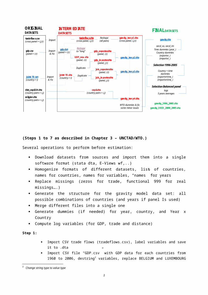
(Steps 1 to 7 as described in Chapter 3 – UNCTAD/WTO.)

Several operations to perform before estimation:

Download datasets from sources and import them into a single software format (stata dta, E-Views wf,..)

Homogenize formats of different datasets, list of countries, names for countries, names for variables, “names” for years

Replace missings (zeros for trade, functional 999 for real missings….) Generate the structure for the gravity model data set: all possible combinations of countries

(and years if panel Is used) Merge different files into a single one Generate dummies (if needed) for year, country, and Year x Country Compute log variables (for GDP, trade and distance)

Step 1:

Import CSV trade flows (tradeflows.csv), label variables and save it to .dta Import CSV file “GDP.csv” with GDP data for each countries from 1960 to 2006, destring2

variables, replace BELGIUM and LUXEMBOURG by BENELUX, compute BENELUX GDP with the sum of both countries and change names for year variables save it in .dta format

Import txt file “joinwto.txt” with year of accession for each country, fix some minor problems 3 and save it in .dta format

Open STATA CEPI2244 datafile containing distances and other interesting variables (for the GRAVITY equation), fix BENELUX problem, drop cases where IMPorter=EXPorter, collapse5 database, change some variable names, label some other variables and save it in .dta format

Basically, at the end of that Step 1, four different STATA files are labeled and stored in the default directory:

1. tradeflows.dta (endogenous variable) in a Panel dataset for YEARS and PAIRS of countries in LONG format

2 Change string type to value type 3 Merge BEL and LUX into BLX because trade data only include BLX data. Change Democratic Republic of Congo code COD by the code ZAR (the one used in trade data).4 Detailed information of each variable could be found at http://www.cepii.fr/pdf_pub/wp/2011/wp2011-25.pdf (pg.11 for “distw” y “distwces” measures) 5 Create a summary statistics dataset with a set of fields (droping the rest) merging info with identical record ID (BLX in our case, for instance)

2

2. joinwto.dta (for the explanatory variable “wtoaccesion”) in a Cross Section dataset for INDIVIDUAL countries

3. GDP.dta (from GDP.csv for explanatory variables GDP’s) in a Panel dataset for YEARS and INDIVIDUAL countries in WIDE format

4. CEPII.dta (other explanatory variables in LONG format) in a CROSS SECTION dataset for PAIRS of countries

3

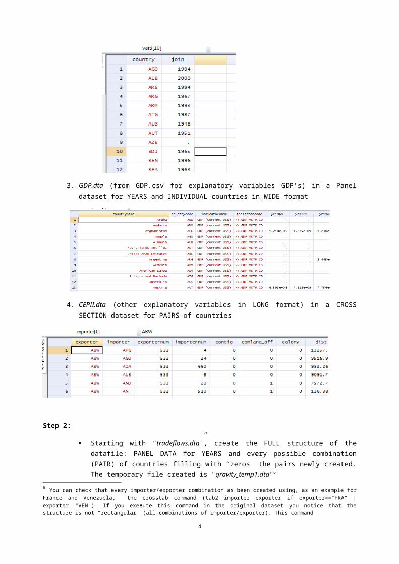
Step 2:

Starting with “tradeflows.dta”, create the FULL structure of the datafile: PANEL DATA for YEARS and every possible combination (PAIR) of countries filling with “zeros” the pairs newly created. The temporary file created is "gravity_temp1.dta"6

Step 3:

Reshape GDP.dta to LONG Panel set and create a duplicate (GDP is going to be used as both importers’s GDP and exporter’s GDP)

reshape long stub, i(i) j(j)\

j new variablereshape long yr, i(countrycode) j(year)rename yr gdp

And MERGE those two new files (“GDP_exporter.dta” and “GDP_importer.dta”) with "gravity_temp1.dta" in "gravity_temp2.dta" keeping those observations (PAIRS of countries) with information in both files.

6 You can check that every importer/exporter combination as been created using, as an example for France and Venezuela, the crosstab command (tab2 importer exporter if exporter=="FRA" | exporter=="VEN"). If you execute this command in the original dataset you notice that the structure is not “rectangular” (all combinations of importer/exporter). This command

4

MERGE “joinWTA.dta” with that file adding new variables: join_exporter and join_importer . The new temporary file created is "gravity_temp3.dta"

Step 4:

MERGE data of both two new files “CEPII.dta” (previously saved) and “religion.dta” with the previous. The new temporary file created is "gravity_temp4.dta"

Step 5:

Create WTO accession dummies depending on whether one, none or both countries are members of WTO or not (onein, nonein, bothin)

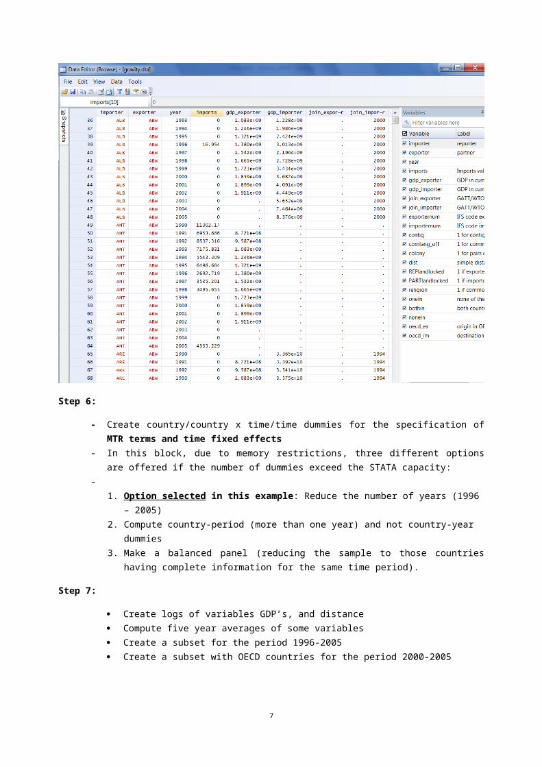
The new PERMANENT file created is "gravity.dta" and basically contains the core dataset (endogenous and exogenous variables, except for country/country x time/time dummies and some lasting transformations)

The structure of the main dataset is shown in the next screenshot: Each row contains a trade flow (import) and the variables for the gravity equation (GDPS, and the terms for barriers and incentives) EXCEPT FOR MRT’S dummies.

5

Step 6:

- Create country/country x time/time dummies for the specification of MTR terms and time fixed effects

- In this block, due to memory restrictions, three different options are offered if the number of dummies exceed the STATA capacity:

-1. Option selected in this example: Reduce the number of years (1996 – 2005)2. Compute country-period (more than one year) and not country-year dummies 3. Make a balanced panel (reducing the sample to those countries having complete information for

the same time period).

Step 7:

Create logs of variables GDP’s, and distance Compute five year averages of some variables Create a subset for the period 1996-2005 Create a subset with OECD countries for the period 2000-2005

2.- ECONOMETRIC ESTIMATIONS OF GRAVITY EQUATIONS

REG1: ESTIMATE A LOG-LOG CROSS SECTION BASIC REGRESION FOR OECD COUNTRIES 2000 AND 2005, WITHOUT MRT’s AND PERFORM SOME BASIC CHECKS

6

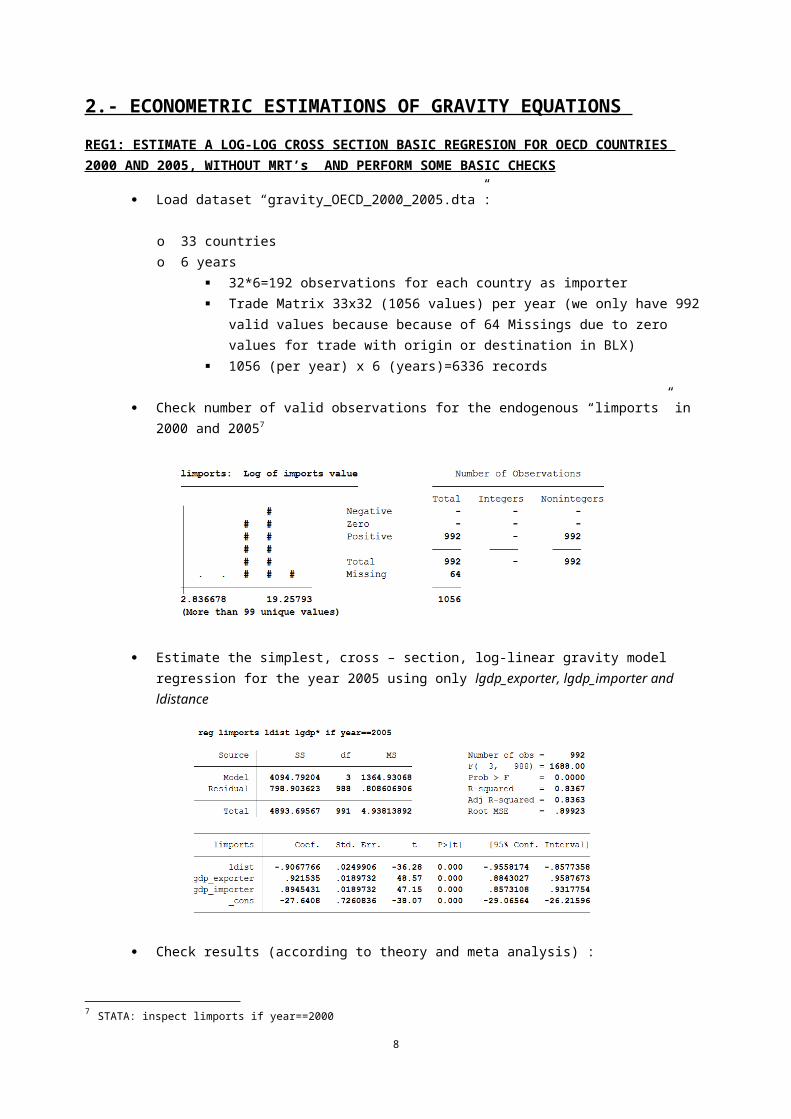
Load dataset “gravity_OECD_2000_2005.dta”:

o 33 countrieso 6 years

32*6=192 observations for each country as importer Trade Matrix 33x32 (1056 values) per year (we only have 992 valid values because

because of 64 Missings due to zero values for trade with origin or destination in BLX) 1056 (per year) x 6 (years)=6336 records

Check number of valid observations for the endogenous “limports” in 2000 and 20057

Estimate the simplest, cross – section, log-linear gravity model regression for the year 2005 using only lgdp_exporter, lgdp_importer and ldistance

Check results (according to theory and meta analysis) :

o High R2 shows the good fit that is frequently found in many empirical gravity modelso Covariates are significant8 and have correct signs o Theory predicts a value around 1 for GDP’s elasticities (both importer and exporter) o GDP’s:

A difference between origins GDP and destination GDPs is expected, a lower estimation for importer GDPs would suggest evidence of home market effects (due to barriers to entry or national product differentiation).

Although both estimations are close to one, maybe statistically different from 1 which might be a finding of interest9

7 STATA: inspect limports if year==20008 Be aware of the “problem” of the large sample size we normally use in gravitational estimations.9 Giving some space for interesting hypothesis about particular dynamics Output Imports / Exports.

7

o Meta-Analysis shows that distance coefficient is also around -1 (proving that distance is a significant obstacle to bilateral trade)

META analysis for 2500 gravity equations estimations.Table extracted from Head, K., & Mayer, T. (2013). Gravity equations: Workhorse, toolkit, and cookbook.

Handbook of international economics, 4.

Check if trade elasticity is significantly more sensible to trade barriers (proxied just by distance in this simple specification) in 2005 than in 2000

o Procedure: compare basic estimation for different years (2000 Vs 2005) using seemingly unrelated estimation (STATA suest10 command)

o It looks like no statistical difference exists comparing 2000 and 2005 estimates.

REG2: ESTIMATE ANOTHER CROSS SECTION REGRESSION INCLUDING ADDITIONAL REGRESSORS

Estimate, with robust inference, for 2005 adding more variables (and using robust estimation to adjust heteroskedastcity):

reg limports contig comlang_off onein colony REPlandlocked PARTlandlocked religion ldist lgdp* if year==2005, robust

10 Seemingly unrelated estimation procedure combines the estimation results (parameter and variance matrices) in one parameter vector and simultaneous (co)variance matrix. The procedure is done after the isolated estimation of each equation. The idea behind this reasoning is that error terms in different equations might be correlated, and that may impact in the estimated covariance of parameters and thus in every cross-model hypothesis concerning parameters of those different equations.

8

o “onein” coefficient cannot be estimated (only zero values), and the same for “bothin” (only value 1) (tab onein if year==2005)

Compare REG1 and REG2 regressions11. Check elasticities obtained:

o GDP’s coefficients for exporter and importer appear to be slightly overestimated (biased) in the first regression. We will always expect that kind of bias for the simplest estimation but the size, and even the sign of this bias depends on the particular nature of relationship between omitted variables (mostly related to trade resistance / incentive) for the particular case of countries comprised in the sample.

o Adjacency coefficient (“contig”) usually lies in the vicinity of 0.5 (Head, K 2003) suggesting that trade is around 65%12 higher as a result of sharing a border. That means that the omission of this simple variable, may cause (as in our case) an upward bias (in absolute value) in distance parameter (both are negatively related to each other).

o Contiguity and common language effects seem to have very comparable effects, with coefficients around 0.5. (Head, K., & Mayer, T. (2013), see table above)).

11 For that, it is useful to use “eststo” command (download it first if not already installed) 12 Remember that, in a log-log model, raw coefficients for dummies do not represent elasticities (% changes). The elasticity can be easily derived with Exp(β)-1, so for a coefficient of 0.5 we get exp(0.5)-1=0.648.

9

o According to some papers, common links (language, colony,…) may cause very significant rises in trade (up to two, three times or even more…). Colonial links are not significant in our regression given the particular nature of the sample (only OECD countries included)

o “Landlocked” variables are weakly significant. Small and positive coeff for exporters and much more important in size for PARTNER (importer) resulting, in that case, in a reduction of imports of around 42% (coeff.=0,357).

REG3: ADDING DUMMIES TO CONTROL FOR MTR’s EFFECT

According to Meta – Analysis (table shown before), gravity models estimated without controlling for MRT terms are biased (comparison between “all gravity” and “structural gravity” sections)

REG. 3.1 Try to estimate previous REG2 for a cross section in 2005, with robust inference, adding country dummies importer_* and exporter_* to control for MTR. Compare this estimation with the previous one 13 (without MRT’s terms).

-

o Important differences appear for common coefficients.

In the case of distance (“ldist”) elasticity is greater / stronger than the previous one and well above “1” (as expected according to the MetaAnalysis)

Contiguity is no longer significant Common language and colonial ties coefficients also changed their values although not

their significance test

o Given that importer_* and exporter_* are country specific (not pair specific) perfectly correlate with other country specif variables such as REPlandlocked PARTlandlocked and lgdp_importer lgdp_exporter so, as expected, after adding country dummies, we CAN NO LONGER estimate the parameters for other country level variables (GDP, *landlocked)14

13 To compare common coefficients using “esttab”, remember to store this equation into memory [STATA: eststo est2] and then compare common coefficients dropping MRT’s dummies *exporternum, *importernum [STATA: esttab, r2 ar2 se scalar(rmse) drop(*exporternum *importernum)]14 A better way to say it is that those coefficients for country dummies show the aggregated value of ALL the country specificities.

10

o Notice that, instead of using country DUMMIES, an alternative solution might be to compute remoteness indexes as detailed in the introductory document (DOC1).

Using the remoteness index is far from a perfect solution. This computation is very not well founded in any theoretical derivation and, at the same time, distance measure should not be the best way of measuring economical remoteness15.

o Trying the estimation with remoteness indexes: -

you will get estimations of country specifics because, contrary to using dummies, we will not have just ONE variable per country, but two SINGLE variables with remoteness computations for importers and exporters

according to literature, the REMOTENESS coefficients are greater than 0 (holding the rest fixed, the more isolated two countries are, the more they trade)

some variables change significance and distance appear to increase elasticity

15 Originally, Head and Mayer's (2000) remoteness variable considered the full range of potential suppliers to a given importer, taking into account their size, distance and relevant costs of crossing the border.

11

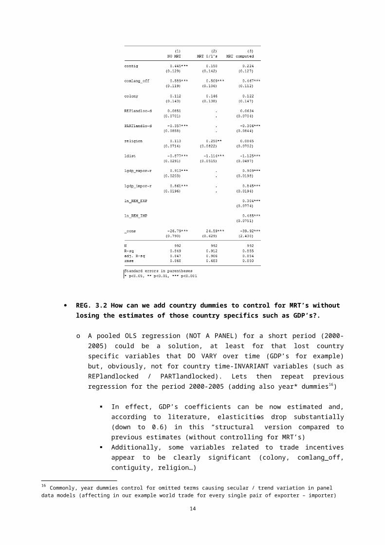
REG. 3.2 How can we add country dummies to control for MRT’s without losing the estimates of those country specifics such as GDP’s?.

o A pooled OLS regression (NOT A PANEL) for a short period (2000-2005) could be a solution, at least for that lost country specific variables that DO VARY over time (GDP’s for example) but, obviously, not for country time-INVARIANT variables (such as REPlandlocked / PARTlandlocked). Lets then repeat previous regression for the period 2000-2005 (adding also year* dummies16)

In effect, GDP’s coefficients can be now estimated and, according to literature, elasticities drop substantially (down to 0.6) in this “structural” version compared to previous estimates (without controlling for MRT’s)

Additionally, some variables related to trade incentives appear to be clearly significant (colony, comlang_off, contiguity, religion…)

16 Commonly, year dummies control for omitted terms causing secular / trend variation in panel data models (affecting in our example world trade for every single pair of exporter – importer)

12

REG. 3.3. What if we now add country x time dummies allowing for MTR time variants? (in the previous regression, MRT terms were supposed to be constant over time)

o The answer is that, given that MRT’s now varies over time, we lose again the estimate of country specific time variant variables (such as GDP’s)

REG. 3.4. What if we now add country-pair dummies allowing to control for paired heterogeneity?

o This is weird, because adding “pairid” fixed effects does not allow to estimate the coefficients for any “country pairs” such as distance, colony, onein,…..

o SO IF WE CONTROL FOR ALL FIXED EFFECTS AT THE SAME TIME (COUNTRY, YEAR, COUNTRY X YEAR, AND COUNTRY-PAIRS) WE THEN LOSE THE REST OF PARAMETERS (except for fixed effects)

13

REG4: PANEL DATA (Step 8 in UNCTAD-WTO document)

Adding country pairs dummies in a POOLED estimation is somehow equivalent to the use of a panel data estimation with fixed effects but we are going to try with a pure PANEL estimator.

Set panel data structure (remember that the panel observation refers to “ij” pairs) Estimate a simple panel data FIXED effects (to control for bilateral MRT’s (including, also, time effects)

o We have to notice again that, controlling with FE for bilateral MRT’s terms we will be unable to estimate coefficients for every TIME INVARIANT bilateral variables both for “ij” pairs (such as distance, colony, common language, FTA) or simply at the level of “i” and/or “j” (such as landlocked)

o Using RANDOM Effects, we may estimate every coefficient (missed with FE) but, as always when we move from FE to RE, at the risk of biased estimates:

14

Check the possibility of RE Vs FE (using a simple Haussman Test)

o Apparently, RE is not the right option so we need to stick to fixed effects.

15