video-based network-wide surrogate safety analysis to

Video-based Network-wide Surrogate Safety Analysis to Support a Proactive Network 1 Screening Using Connected Cameras: Case Study in the City of Bellevue (WA) United 2

States 3 4 Lana Samara 5 Project Coordinator 6 Transoft Solutions 7 1176 Bishop Street, Room 302 8 Montreal, Canada, H3G 2E3 9 Email: [email protected] 10 11 Paul St-Aubin, Ph.D., P.Eng 12 Senior Product Manager 13 Transoft Solutions 14 1176 Bishop Street, Room 302 15 Montreal, Canada, H3G 2E3 16 Email: [email protected] 17 18 Franz Loewenherz, M.Sc 19 Principal Transportation Planner 20 City of Bellevue – Transportation Department 21 450 110th Avenue NE 22 Bellevue, Washington, 98004 23 Email: [email protected] 24 25 Noah Budnick 26 Senior Director, Programs & Operations 27 Together for Safer Roads 28 97 North 10th St #2A 29 Brooklyn, NY 11249 30 Email: [email protected] 31 32 Luis Miranda-Moreno, Ph.D. 33 Associate Professor 34 Department of Civil Engineering, McGill University 35 MacDonald Engineering Building 36 817 Sherbrooke St. W., Office 278-A 37 Montreal, Canada, H3A 2K6 38 Email: [email protected] 39 40 Word Count: 6868 + 2 tables (250 words per table) = 7368 words 41 42 43 Submitted [August 1st 2020] 44

mailto:[email protected]





Samara, St-Aubin, Loewenherz, Budnick, and Miranda-Moreno

2

ABSTRACT 1 Surrogate road safety approaches, as part of road improvement programs, have gained traction in recent 2 years. Thanks to emerging technologies such as computer-vision and cloud-computing, surrogate methods 3 allow for proactive scanning and detection of safety issues and address them before collisions and injuries 4 occur. The objective of this paper is to propose an automated and continuous monitoring approach for 5 road network screening using connected video cameras and a cloud-based computing analytics platform 6 for large-scale video processing. Using the wide network of traffic cameras from cities, the proposed 7 approach aims to leverage video footage to extract critical data road network screening (ranking and 8 selection of dangerous locations). Using the City of Bellevue as an application environment, different 9 safety metrics are automatically generated in the platform such as traffic exposure metrics, frequency of 10 speeding events, and conflict rates. Using Bellevue’s camera network, the proposed approach is 11 demonstrated using a sample of 40 cameras and intersections. The results and platform provide a 12 proactive tool that can constantly look for dangerous locations and risk contributing factors. This paper 13 provides the details of the proposed approach and the results of its implementation. Directions for future 14 work are also discussed. 15 Keywords: Computer vision, video-based traffic monitoring, network screening, surrogate safety, vision 16 zero 17


3

INTRODUCTION 1 Road safety has been a fundamental concern globally, costing most countries around 3% of their 2

gross domestic product. Road crashes kill approximately 1.35 million people annually, placing them in 3 the top ten causes of death, and making them the leading non-disease cause of death world-wide. More 4 than half of these deaths are among vulnerable road users, making them more high risk (1). In the United 5 States, the annual death rate due to road crashes is 38,000 (resulting in 12.4 deaths per 10,000 6 inhabitants). 4.4 million additional road users have injuries requiring medical attention. This amounts to 7 $871 billion in societal and economic costs, making the United States the most affected high-income 8 country by the consequences of crashes. In addition, the number of pedestrian and cyclist fatalities have 9 been on the rise since 1990 (2). 10

In response to these road safety concerns, many cities have adopted road safety programs to 11 achieve Vision Zero. One of the main goals of Vision Zero is to eliminate traffic fatalities and serious 12 injuries to ensure that all road users can safely move around their communities. This concept was 13 introduced in 1995 and has since been adopted in 24 countries world-wide and in over 40 cities in the 14 United States alone (3). Vision Zero recognizes that road users make mistakes or can be confronted with 15 dangerous situations and that public roads should be designed to accommodate for these modes of 16 failure—in the jargon of safe systems engineering, public roads should be fault tolerant. 17

Two major components of the program include managing safe travels and collecting, analyzing, 18 and using data to understand the causes of traffic deaths and their effects. This requires the establishment 19 of safety programs and goals that include educational, enforcement, and engineering countermeasures. 20 This implementation requires following the road safety management process (RSMP) which offers a 21 systematic approach to the site identification, improvement selection, and evaluation (4). The process 22 starts with a network screening process to determine the locations of interest. Once the locations are 23 selected, diagnosis is performed to identify the crash-risk contributing factors in order to then select the 24 proper countermeasures. A cost-benefit analysis is then performed, and projects are prioritized. Finally, 25 safety effectiveness evaluations are performed at multiple levels – on the project level, countermeasure 26 level, and/or program level (5). 27

Several steps in the RSMP are currently heavily reliant on the use of crash data. This creates a 28 significant obstacle for achieving Vision Zero, due to the long time required to obtain this data, in 29 addition to the issues surrounding data gaps, under-reporting, cross-jurisdictional inconsistencies, and the 30 ethical concerns with acting on crashes only after they happen. This necessitates the use of more proactive 31 measures, known as surrogate safety measures. These measures are used to reflect the current state of 32 road safety by providing information on crash risk (6). Due to the granular nature of the data required to 33 provide these measures, various technologies have been used in the context of diagnosis and safety 34 evaluation. These include cameras, LIDAR, and GPS, each with its documented advantages and 35 shortcomings (7)(8)(9)). 36

Additionally, obtaining surrogate safety measures for network screening purposes adds another 37 layer of complexity as massive amounts of data need to be derived in a systematic and continuous 38 manner. Previous works have investigated the use of GPS data for network screening purposes with 39 documented success (9). However, despite the latest research developments, a limited number of studies 40 have explored the use of computer vision and available city infrastructure (network of traffic video 41 cameras and management center facilities) to perform continuous and automatic network screening. 42 Traditional network screening methods can only be performed at discretized intervals on a scale of years. 43 With the use of connected city cameras, computer vision, and surrogate safety measures, network 44 screening can be performed on a daily-, hourly-, or minute-by-minute-basis if desired. This new approach 45 enables city engineers to monitor changes in traffic patterns and respond proactively to emerging safety 46 warnings with countermeasure improvements. 47

The objective of this paper is to introduce the concept of automated and continuous monitoring 48 for road network screening using available infrastructure (connected cameras and cloud computing) and a 49 video analytics software solution referred to as BriskLUMINA. Using the wide network of traffic cameras 50 from cities, the proposed concept aims to leverage video footage to obtain useful data that can be 51


4

searched, managed, and used to provide city road safety authorities with detailed information on traffic 1 volumes, speeds, conflicts and other driver behaviors so that they can respond more rapidly to road safety 2 issues. This paper presents the concept using the City of Bellevue as an application environment and 3 using various traffic flow and safety metrics (such as traffic exposure, over-speeding, near-miss indicators 4 based on frequencies and rates, etc.). This screening provides the City with data on which locations 5 experience road safety issues for motorized and vulnerable road users for a particular time, day, or traffic 6 movement. 7 8 LITERATURE REVIEW 9

In recent years, many communities have been looking beyond crash records for data-driven safety 10 analysis. Studying collision data is reactive; safety evaluation takes place after collisions occur, making it 11 nearly impossible to achieve the goal of zero traffic deaths and serious injury collisions. Additionally, the 12 infrequent nature of traffic collisions necessitates years of observation to achieve statistical significance 13 — up to 5 or even 10 years of data in the cases of studies involving single sites and/or low-traffic volume 14 locations, during which these locations may change significantly. Furthermore, it is well-documented that 15 traffic crashes and injuries are under-reported in many localities and there are societal barriers in using the 16 general public to test unknown safety countermeasures (10). 17

These concerns have led Vision Zero cities to use surrogate safety measures to proactively 18 identify locations that have a high risk of crashes but where the risk has not yet resulted in actual crashes. 19 These surrogate safety metrics are collected from analysis of road-users’ trajectory data and near-collision 20 data. A wide variety of surrogate safety measures exist, including speed, delay, violations, deceleration 21 distribution, etc. (6). Two very popular metrics of crash risk are divided into measures of proximity and 22 crash severity with time-to-collision (TTC) and post-encroachment time (PET) being measures of 23 proximity and speed, and with acceleration, object size, and collision angle being measures of severity. 24 TTC is “the time required for two vehicles to collide if they continue at their present velocity and on the 25 same path” (11). PET is the time difference between when the first road user leaves the conflict point and 26 the second road user arrives at the conflict point (12). TTC is computed continuously and depends on the 27 predicted motion of the two road users whereas PET requires the two road users to have intersected paths 28 at some point. TTC is better suited for road users whose paths coincide for more than a single point of 29 their trajectories such as two road users originating from the same lane or merging into the same lane. 30

Many research groups have researched and developed the applications of computer vision to 31 surrogate safety with promising results (13). The use of video analytics to obtain surrogate safety data has 32 been growing in popularity due to the richness and granularity of the data that can be obtained. This 33 approach offers an alternative method of obtaining the desired metrics that is relatively inexpensive and 34 quick. Unlike traditional traffic safety evaluation methods, video-based monitoring is detailed enough to 35 identify near-crashes, classify road user types and their movements, and detect speeding infractions and 36 lane violations. Cameras capture high-resolution data for all road users and modes of transportation 37 within the field of view of the camera, compared to GPS sensor data, which only capture some of the road 38 users (8)(9). Unlike LIDAR, cameras are relatively easy to deploy and maintain alongside a traditional 39 surveillance system (7). Lastly, videos are easy for people to review and understand, unlike many other 40 data collection technologies that simply provide numerical data. 41

Despite recent developments in the literature on surrogate safety, most of the work has been 42 focused on the proposition of new surrogate safety methods or the use of surrogate approaches for safety 43 diagnosis or before-after studies (14)(15). Very little work has been published using large-scale studies. In 44 particular, to our knowledge, no studies have been published using a large network of connected cameras 45 for proactive network screening – which is the first step of the classical RSMP. 46 47 METHODOLOGY 48 The implementation of the network-wide continuous monitoring system with connected cameras 49 consisted of several steps. For the methodology implementation, the City of Bellevue’s connected camera 50 network was used as an application environment. First, the locations at which the analysis was to be 51


5

performed were selected. Then, the analytics system was deployed at those locations and calibration was 1 performed. Finally, the numerical and visual data were generated and then analyzed. 2

3 Location Selection 4

The criteria for location selection were: 1) presence of a camera at the road segment, 2) camera 5 having an appropriate field of view, 3) rank with respect to the High Injury Network (16), and 4) variation 6 in land use, urban density, and road geometry. 7

The City of Bellevue’s up-to-date camera infrastructure and modern traffic management centers 8 ensured the smooth implementation of the system. The city has a network of high resolution connected 9 cameras at approximately 110 of its 200 intersections with fibre optic video streaming capabilities. All 10 cameras are mounted on traffic signals or poles between 20 and 40 feet high making them appropriate for 11 this type of deployment. 12

The presence of a camera was the most important selection criteria, narrowing down the number 13 of possible locations. Of these locations, the fields of view of all the cameras were assessed to eliminate 14 the locations where the camera’s field of view did not cover the entire intersection. Another important 15 criterion was the inclusion of a variety of locations along the City’s High Injury Network (HIN) (and with 16 a variety of ranks within that network – high, medium, and low) and locations not on the HIN (16). 17 Additionally, the intersections selected were also geographically spread out throughout the city, had 18 varying urban densities, and different land uses. Finally, the selection of intersections took into 19 consideration varying road geometry and infrastructure. 20 21 Video-based Traffic Monitoring Platform Deployment 22

After the locations of interest were finalized, vision-based traffic monitoring was performed. This 23 process involves 1) livestreaming the video footage, 2) calibration and validation, 3) video-based AI 24 processing and safety analysis, 4) quality control and data filtering, and 5) presentation of analytics results 25 on the dashboard. This process is depicted in Figure 1. 26 27

28 Figure 1 Video-analytics process for safety analysis 29 30

The video footage from the intersections of interest was live streamed. The intersection meta-31 data, alongside a short sample of video footage, was then input on the platform to perform the calibration. 32 During the calibration process, a coordinate transformation is performed using the camera view and an 33 aerial image for mapping purposes. The portion of the camera’s field of view of interest is then isolated 34 and the relevant movements are defined. Once calibration is complete, result validation is performed to 35 ensure accurate results (proper mapping and movement definition). Additionally, random 15-minute 36 manual traffic counts are compared to automatic counts to ensure count accuracy. 37

Once the validation process is complete, the video footage can be continuously processed. During 38 processing, computer vision is used to detect, classify, and track each of the road users in the traffic 39 stream. For this purpose, state-of-the art algorithms have been developed and integrated in the 40 BriskLUMINA platform. (17) Once the detection and tracking algorithms are implemented, the platform 41


6

automatically generates a set of traffic flow and safety outcomes. This includes graphs, heat maps, and 1 video clips as well as risk indicators at different levels (scenario and intersection level). The results are 2 then quality controlled to ensure a high-level of accuracy, removing any false positives in the outcomes. 3 Once all of this is complete, the results are available on the online safety dashboard. 4 5 Output Analytics 6

The outputs from the video-analytics cloud platform (BriskLUMINA) provide information on 7 traffic flow (volumes and speed measures) and safety (in the form of near-misses and violations). The 8 outputs of the video analytics provide granular information on every single road user observed in the 9 video footage as well as more aggregate data at the scenario and intersection level in the form of charts 10 and heatmaps. Some of the typical outputs of the analytics are provided in Figure 2. 11

12

13 Figure 2 Output analytics 14 15 The following data was used throughout the network screening process. 16

• Traffic volumes: Data is available on every road user captured. The road users observed are 17 bound by the field of view of the camera. Depending on the intersection, this extends between 0 18 to 30-feet from the stop line of each approach. Each road user is identified as a road user type 19 (truck, bus, car, motorcycle, cyclist, pedestrian, etc.) and is associated with a movement (eg. 20 northbound through or East crosswalk). The data can be obtained on more aggregate bases, such 21 as on a 15-minute, daily, site, or network basis. 22


7

• Speed measures: For each road user, speed measures are calculated on a frame by frame basis. 1 Ultimately the speed vector assigned to each road user can be used to compute mean, median 2 speed, 85th percentile or other measures of speed using their trajectory data. Just as with the 3 volume data, this data can be obtained for each road user or aggregated over various desired 4 parameters. 5

• Near-misses or conflict events: Near-miss events are quantified using PET as the indicator (or 6 optionally, also using TTC). Data is available for all events that involve the interactions of two 7 road users with a PET < 10 s, for relevant scenarios. Relevant scenarios are scenarios involving 8 two road users whose trajectories intersect, excluding events involving two pedestrians. In this 9 paper, events with PETs < 2 s are denoted as critical conflicts. Critical conflict rates were 10 calculated based on the total number of critical conflicts per 10,000 road users for the study 11 period. 12

• Speeding events: Speeding violations or events, as defined by the traffic video analytics output, 13 occur when a road user is traveling above the posted speed limit for more than 20% of their 14 moving trajectory. Speeding is limited to motorized road users and uses the speed limits of 15 through movements as the assigned speed limit for the intersection. Anyone driving above the 16 speed limit will have an excessive speed value, defined as the median speed value of the vehicle’s 17 speeding trajectory. In this paper, speeding incidence rates were calculated based on the total 18 number of speeding road users per 10,000 road users for the week of the study period. Other 19 traffic violations can be extracted in an automated way but this application is limited to over-20 speeding. 21

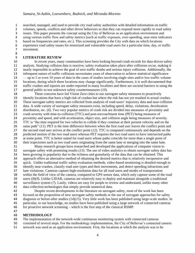
22 Figures 3 a-e show some sample platform outputs for the week of analysis at different study 23

locations. Figures 3.3a and b show the detected trajectories superimposed onto the camera’s field of view. 24 Figure 3.3c shows a conflict heatmap, indicating the frequency of more critical conflicts at specific 25 locations within the intersection. Figure 3.3d aggregates all the road user speeds to show a speed heatmap. 26 Lastly, Figure 3.3e shows a screenshot of a car exceeding the speed limit by more than 30 mph. 27

28

29 a) Trajectories by movement b) Trajectories by Road User Type 30

31 c) Conflict heatmap d) Speed Heatmap 32


8

1 e) Speeding violation video 2 3

Figure 3 Sample analytics platform outputs 4 Analyses 5

In addition to looking at the raw-data indicators mentioned before (e.g., the frequency or rates of 6 conflicts or speeding events), a statistical regression model can be used to estimate the frequency of 7 events for each intersection after controlling for other factors. In this case, a multi-level regression model 8 is used to perform a network-wide analysis. Multiple geometric and non-geometric variables were 9 considered as explanatory variables when fitting these models. The explanatory variables include urban 10 density (high or medium), land use (commercial or residential), whether or not a school is present within 11 less than 0.125 miles from the intersection, road user types (car driver, bus or truck operator, 12 motorcyclist), road user movement (through, left turn, or right turn), protected vs non-protected left turns, 13 pedestrian traffic phasing, number of lanes, lane width, crosswalk width, presence of bike infrastructure 14 (dedicated bike path, shared bike path, both, or neither), time of the day, and days of the week. 15

The multilevel regression analysis was estimated with intersection fixed and random effects using 16 the independent variables as surrogate safety measures. 17 18

𝑦𝑖 = 𝛽0 + 𝛽1 𝑥𝑖 1 + 𝛽2 𝑥𝑖2 + ⋯ + 𝛽𝑝 𝑥𝑖𝑝 + 𝛼𝑍𝑖 + 𝜀𝑖, i=1, 2,…..,n 19

Where: 20 yi – surrogate safety measure of interest for site i, for all conflicts 21 xij – regressor for explanatory variable j 22 βj – coefficient for explanatory variable j 23 𝛼Zi - fixed effects error for site i 24 εi – random error of the regression estimate 25 26

Using the expected frequency of events at the site level, the sites under study were ranked to identify the 27 most dangerous locations according to the specific indicator. 28 29 APPLICATION 30

Between 2009 and 2018, 66% of all fatal and serious-injury collisions in the City of Bellevue 31 occurred along just 9% of streets (16). Vulnerable road users (pedestrians and cyclists) made up 5% of all 32 collisions during this time but comprised 46% of all serious injuries and fatalities. An analysis of the 33 collisions indicated that the following five road user behaviors contributed to 70% of all fatal and serious 34 injuries: driver’s failure to yield to a pedestrian, failure to grant right-of-way to a motorist, driver 35 distraction, intoxication, and speeding (16). In response to these road safety concerns, the City of 36 Bellevue passed a Vision Zero resolution in 2015 to strive to eliminate traffic fatalities and serious 37 injuries by 2030. In 2019, the City of Bellevue conducted a citywide network screening analysis to better 38 understand the factors that impact the safety of its transportation system and leverage this insight to 39 identify improvements and evaluate outcomes. Camera footage was analyzed to obtain data about 40 surrogate safety indicators including road user speeds and near-misses. Results are used to validate road 41


9

improvements, determine high-risk locations, and determine the most severe conflicts and interactions at 1 an intersection. 2

For the implementation of the proposed approach, a sample of 40 intersections were selected, from 3 the City’s 200 intersections. Figure 4 depicts the study intersections. The selection was based off of 4 the aforementioned factors: 5 • All intersections were signalized with a connected camera with the appropriate field of view. 6 • From those, 34 are four-legged intersections, 5 are three-legged, and 1 is five-legged. 7 • Most of the intersections (31) were part of the High Injury Network. 8 • The majority of the intersections (31) were not in the downtown area, defined here as the area 9

bordered by Main St. & NE 12 and 100th Ave & 112th Ave. 10 • Priority was given to intersections located in commercial areas given the high pedestrian 11

presence. In the sample, 28 intersections were located in commercial areas as opposed to 12 residential areas. 13

• 28 intersections were in medium density locations (suburbs, big-box stores, and/or factories) 14 while the rest were in high density locations (multi-story dwellings and/or businesses). 15

16

17 Figure 4 Study locations 18 19 Results 20

Video data was processed using the analytics platform defined earlier. For each intersection, 112 21 hours of video data (6AM to 10PM) were collected and automatically processed for a total of 4,500 hours 22 of video footage. This corresponds to seven consecutive days of data from September 13th to 19th, 2019. 23 Once data was streamed to the cloud analytics platform, each camera was calibrated and detection/ 24 tracking algorithms were implemented. This was followed by the generation of traffic flow and safety 25 analytics metrics. A multitude of analyses can be performed on the data obtained; however, the section 26 will provide a set of outcomes for illustrative purposes. 27 28 4.1.1 Volumes 29

During the week of data collection, over 8.25 million road users were observed. From the total, 30 97.3% were motorized road users and 2.7% were vulnerable road users (2.6% pedestrians and 0.1% 31 cyclists). Figures 5 a-c show the concentration of each road user type across the network. 32


10

1 a) Motorist volumes across network b) Bicyclist volumes across network 2 3

4 c) Pedestrian volumes across network 5 Figure 5 Concentration of each road user across network 6

7 The average total vehicular volume per intersections was between 0.2 and 0.25 million for the 8

entire week of analysis. The 2 intersections with the highest volumes, at around 0.4 million, were 112th 9 Ave & NE 8th St and 116th Ave & NE 8th St. These high volumes were observed as both intersections 10 are adjacent to interstate ramps. Pedestrian volumes were less uniform throughout the study locations. 11 Over half of all the pedestrian volumes observed were at four downtown, high density intersections 12


11

(Bellevue Way & NE 8th St, 108th Ave & NE 8th St, 108th & NE 4th St, and Bellevue Way & Main St). 1 For more than two-thirds of the selected locations, pedestrian volumes made up less than 2% of the total 2 traffic. Cyclist volumes were very low throughout all study intersections, and cyclists made up more than 3 1% of road user volumes at only 2 intersections (116th Ave NE & Northup Way and 100th Ave & Main 4 St). 5 6 Speeds 7

The speed for all the road users was obtained on a road user basis and was aggregated for a 8 network-wide analysis by road user type and movement type. This section looks at the temporal variation 9 in through vehicular speeds by land use, speed limit, and intersection location along the HIN. Other 10 analyses can be performed by looking at different road users and/or turning movements and other metrics 11 such as 85th percentile speeds, free flow speeds, coefficient of variation etc. 12

Figures 6a-c display the temporal variation of through vehicle speeds with respect to different 13 factors. On a network-wide basis, through movement speeds were relatively constant throughout the day. 14 Vehicles at residential locations had higher speeds and fluctuations compared to commercial locations. As 15 would be expected, speeds were lower at intersections with posted speed limits of 30 mph compared to 16 intersections with posted speed limits of 35 mph. Fluctuations in speeds throughout the day were slight 17 for both posted speed limits and do not appear to have a clear correlation with the time of day. Speeds 18 along the HIN were observed to be lower than speeds not on the HIN. This is due to speeds and speeding 19 limits being higher at residential land use and two-thirds of the selected locations not on the HIN were in 20 residential areas. 21 22

23 a) Average speed (mph) by land use b) Average speed (mph) by speed limit 24 25

26 c) Average speed (mph) by High Injury Network 27 Figure 6 Weekday through average vehicle speeds with respect to different factors 28

0

10

20

30

40

50

6:0

0 A

M

7:0

0 A

M

8:0

0 A

M

9:0

0 A

M

10:0

0 A

M

11:0

0 A

M

12:0

0 P

M

1:0

0 P

M

2:0

0 P

M

3:0

0 P

M

4:0

0 P

M

5:0

0 P

M

6:0

0 P

M

7:0

0 P

M

8:0

0 P

M

9:0

0 P

M

Sp

eed

(m

ph)

Total Commercial Residential

0

5

10

15

20

25

30

356

:00 A

M

7:0

0 A

M

8:0

0 A

M

9:0

0 A

M

10:0

0 A

M

11:0

0 A

M

12:0

0 P

M

1:0

0 P

M

2:0

0 P

M

3:0

0 P

M

4:0

0 P

M

5:0

0 P

M

6:0

0 P

M

7:0

0 P

M

8:0

0 P

M

9:0

0 P

M

Sp

eed

(m

ph)

Total 30 mph 35 mph

0

10

20

30

40

50

60

6:0

0 A

M

7:0

0 A

M

8:0

0 A

M

9:0

0 A

M

10:0

0 A

M

11:0

0 A

M

12:0

0 P

M

1:0

0 P

M

2:0

0 P

M

3:0

0 P

M

4:0

0 P

M

5:0

0 P

M

6:0

0 P

M

7:0

0 P

M

8:0

0 P

M

9:0

0 P

M

Sp

eed

(m

ph)

Total HIN non-HIN


12

Conflict Frequency and Rates 1 Near-misses 2

The safety indicator used to quantify near-misses was PET. Approximately 1.5 million events 3 with PETs < 10s were observed across the week of analysis. Figure 7 shows the distribution of the PET 4 values of these events. For this paper, data will be provided based on the number of conflicts with a PET 5 < 2s. This value was selected because it is slightly higher than 1.5s, the average human reaction which is 6 a common threshold use to identify conflicts with a relatively high-risk level, (18)(19) to ensure that no 7 conflicts with a slightly higher reaction time are not overlooked. These will be called critical conflicts 8 hereon. Twenty thousand (1.4% of all interactions) of these events were observed, while more than 80.7% 9 of interactions had PETs between 5 and 10 seconds which is considered to be safe passage. As would be 10 expected, the distribution of conflicts/interactions across the threshold values follows a pyramidal shape. 11 12

13 Figure 7 Distribution of PET value of all events 14 15

Based on the video analytics data, several ranking criteria could be derived for identifying the 16 most prone intersections for safety improvements, this includes critical conflict rates defined as the 17 number of conflicts observed with PETs < 2s per 10,000 road users for the week of analysis. Figure 8 18 presents a map showing the concentration of the total number critical conflict rates per intersection. This 19 map is useful for identifying those intersections with a high frequency of critical conflicts. The map 20 indicates that 7 intersections had more than 150 critical conflicts daily. 21 22

80.7%

13.1%

4.8%

1.4%

Critical Conflicts ( PET < 2 s)

Minor Conflicts (2 s < PET < 3 s)

Potential Conflicts (3 s < PET < 5 s)

Interactions (5 s < PET < 10 s)


13

1 Figure 8 Concentration of critical conflicts across network 2 3

When exploring conflicts by mode, vehicular conflicts made up 97.5% of all critical conflicts 4 observed. Pedestrian conflicts made up only 1.9% of all these conflicts, and cyclist conflicts made up 5 0.6%. Even though cyclists were involved in the least number of critical conflicts, they had the highest 6 critical conflict rates. When comparing the critical conflict rates for each road user, cyclists were 6.5 7 times more likely to be involved in a conflict than a pedestrian and 8.7 times more likely to be involved in 8 a conflict than a vehicle. Additionally, pedestrians were 1.3 times more likely to be involved in a conflict 9 than a vehicle. 10

Depending on the countermeasures or policies in place, hotspot intersections with the highest 11 frequency of a specific conflict scenario can be identified. Figures 9 a-c indicate the frequency of the 12 main conflict scenarios and their frequency for each road user, on a network-basis. The vehicular conflicts 13 were predominantly between through and left turning vehicles. Additionally, pedestrian conflicts with left 14 turning vehicles were also most common. The most common cyclist conflicts were between cyclists and 15 through vehicles. 16

17

18 a) Vehicular conflict scenarios b) Pedestrian conflict scenarios 19 20

1.1%

98.3%

0.6%

Through &

Through Vehicles

Through & Left

Turning Vehicles

Through & Right

Turning Vehicles

26.1%

9.6%64.3%

Pedestrians &

Through Drivers

Pedestrians &

Left Turning

Drivers

Pedestrians &

Right Turning

Drivers


14

1 c) Cyclist conflict scenarios 2 3 Figure 9 Conflicts by scenario for every road user 4 5

Based on the above information, multiple countermeasures can be proposed in the diagnosis stage 6 to address the safety of these scenarios. With respect to vehicle-bicycle interactions, as cyclist volumes 7 were very low throughout the intersections studied, the number of conflicts observed was also low. If the 8 priority is targeting bicycle safety, longer periods of video data could be processed to increase the number 9 of observations. Given the accessibility to video data from connected cameras, extending the period of 10 observation is not an issue. 11

If the interest is to identify hotspots during critical hours of the day, critical days of the week, 12 and/or by land use type, conflict frequency or rates per intersection can be generated per hour or per 13 weekday. For instance, in this sample of intersections, conflict rates were highest in the morning around 7 14 AM and were the lowest after 7 PM. Intersections in residential areas had higher conflict rates than 15 commercial areas throughout the day, as is depicted in Figure 10. 16

17 Figure 10 Hourly distribution of conflict rates by type of land use 18 19 Speeding 20

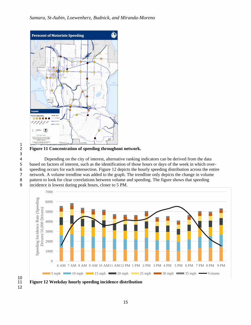
As in the case of conflicts, ranking criteria for hotspot identification could be derived from over-21 speeding events – which are defined based on speed limits for each particular approach when vehicles 22 enter-exit the intersection. Throughout the network, around 870,000 instances of driver exceeding the 23 speed limit were observed, indicating that approximately 10.8 % of motorized vehicles were speeding. 24 The number of road users speeding at each intersection is listed in Figure 11 and the top 5 intersections 25 with the most speeding incidence rate can be identified. 26

71.1%

24.8%

4.1%

Cyclist &

Through Vehicles

Cyclist & Left

Turning Vehicle

Cyclist &

Merging Vehicles

05

1015202530354045

Co

nfl

icts

/10

,00

0 R

oad

Use

rs

Time

All Commercial Residential


15

1 Figure 11 Concentration of speeding throughout network. 2 3

Depending on the city of interest, alternative ranking indicators can be derived from the data 4 based on factors of interest, such as the identification of those hours or days of the week in which over-5 speeding occurs for each intersection. Figure 12 depicts the hourly speeding distribution across the entire 6 network. A volume trendline was added to the graph. The trendline only depicts the change in volume 7 pattern to look for clear correlations between volume and speeding. The figure shows that speeding 8 incidence is lowest during peak hours, closer to 5 PM. 9

10 Figure 12 Weekday hourly speeding incidence distribution 11

12

0

1000

2000

3000

4000

5000

6000

7000

6 AM 7 AM 8 AM 9 AM 10 AM11 AM12 PM 1 PM 2 PM 3 PM 4 PM 5 PM 6 PM 7 PM 8 PM 9 PM

Sp

eed

ing I

nci

den

ce R

ate

(Sp

eed

ing

Dri

ver

s/1

0,0

00

Dri

ver

s)

5 mph 10 mph 15 mph 20 mph 25 mph 30 mph 35 mph Volume


16

Figures 13 a and b display the hourly variation of speeding incidence rates by land use and speed 1 limit. Speeding incidence rates appear to be lowest during the peak hours between 3 and 6 PM. Speeding 2 was more prevalent in residential areas, with 14% of vehicles speeding compared to commercial areas 3 where 10.6% of vehicles were observed speeding. In terms of speeding at locations with different speed 4 limits, speeding incidence rates did not appear to be more prevalent at either location. Looking at the 5 temporal variation, speeding incidence rates were slightly higher at locations with speed limits of 35 mph 6 in the morning; however, later in the afternoon, speeding incidence rates were slightly higher at locations 7 with speed limits of 30 mph. Additionally, vehicular speeding incidence was found to be higher 8 downtown with 15% of the vehicles speeding compared to the areas outside of downtown where 10.5% of 9 the vehicles were speeding. 10 11

12 a) Speeding incidence rates by land use b) Speeding incidence rates by speed limit 13 14 Figure 13 Weekday speeding incidence rates by different factors 15

16 Hotspot Identification 17

To create both the network-wide model for the conflict data, two surrogate safety measures were 18 analyzed, vehicle speed and PET. These two measures were considered as PET alone is insufficient to 19 estimate the injury risk of a potential collision. The modeling approach, as described in the 20 methodological section, involves fitting a multilevel regression model to the data with random and fixed 21 effects at the intersection level. Once alternative models are fitted, the model with the best combination of 22 variables is identified based on goodness-of-fit measures. Using the model outcomes, the expected 23 number of conflicts or rates are estimated after controlling for other variables. This approach is similar to 24 the classical regression approach using safety performance functions and Empirical Bayesian models with 25 observed crash data. 26

The outputs of the network-wide PET and Speed models are listed in Table 1. The model 27 indicated that the top 5 high-risk intersections were 116th Ave NE & Northup Wy, 124th Ave NE & NE 28 8th St, Richards Rd & 26th St, 145th PI SE & SE 16th St, and 130th Ave NE & Northup Wy. 29

With respect to the linear regression model used for the network-wide analysis, lower PETs and 30 higher vehicle speeds are less desirable (i.e. indicative of more high-risk situations). Higher traffic 31 volumes led to a reduction in speed and in PET severity. Speeds were lowest at locations with speed 32 limits of 30 mph followed by 40 mph and then 35 mph. PET values were lowest (indicating more critical 33 interactions) at locations with speed limits of 35 mph, followed by 30 mph and are highest at speed limits 34 of 40 mph. Both the speed and PET models indicated that motorcyclists were the most high-risk road user 35 as they increased the average speed by 1.15 mph and reduced PETs by 0.21 seconds. Through and 36

0

500

1000

1500

2000

2500

3000

3500

Sp

eed

ing I

nci

den

ce R

ate

(

Sp

eed

ing V

ehic

les/

10

,00

0

Veh

icle

s)

Total Commercial Residential

0

500

1000

1500

2000

2500

Sp

eed

ing I

nci

den

ce R

ate

(Sp

eed

ing V

ehic

les/

10

,00

0

Veh

icle

s)

Total 30 mph 35 mph


17

through interactions with PET >2s were observed to be the most prone to higher speeds but happened at 1 higher PETs (closer to 10 s) indicating they were not as critical of conflicts. 2 3 TABLE 1 PET and Speed Network-wide Model Outputs 4

Parameter Coef. Std.

Err. t P>t

95% Conf.

Interval

PE

T M

od

el

1-hour Volumes 0.002 0.0001 32.38 0.000 0.000 0.000

Peak

Hour

0 0 (base)

1 0.055 0.005 11.43 0.000 0.0453 0.064

Day of

Week

Weekday 0 (base)

Weekend -0.034 0.005 -6.68 0.000 -0.0442 -0.024

Speed

Limit

30 0 (base)

35 1.316 -0.037 33.6 0.000 1.244 1.389

40 0.805 0.032 25.13 0.000 0.742 0.867

Road

User

Type

Car -0.064 0.059 -1.14 0.225 -0.183 0.049

Bus 0.079 -0.056 5.34 0.000 0.0499 0.1079

Bicycle -0.143 0.0307 -4.65 0.000 -0.2027 -0.082

Motorcycle -0.207 0.04 -5.12 0.000 -0.286 -0.128

Pedestrian 0 (base)

Truck 0.028 0.0105 2.67 0.007 0.008 0.0490

Scenario

Through & Through 0 (base)

Through & Left Turn -0.661 0.006 -115.95 0.000 -0.672 -0.650

Left Turn & Through -0.780 0.006 -136.71 0.000 -0.791 -0.769

Left Turn & Left Turn 0 (base)

Sp

eed

Mo

del

1-hour Volumes 0.004 0 -22.61 0.000 -0.002 -0.002

Peak

Hour

0 0 (base)

1 -0.617 0.038 -16.83 0.000 -0.689 -0.545

Day of

Week

Weekday (base)

Weekend 0.714 0.039 18.22 0.000 0.637 0.791

Speed

Limit

30 0 (base)

35 10.876 0.283 38.37 0.000 10.32 11.431

40 -7.854 0.246 -31.99 0.000 -8.336 -7.37

Road

User

Type

Car -0.428 0.454 -0.94 0.346 -1.318 1.462

Bus -2.391 0.113 -21.1 0.000 -2.614 -2.169

Bicycle -5.63 0.235 -23.94 0.000 -6.091 -5.169

Motorcycle 1.849 0.309 5.97 0.000 1.241 2.456

Pedestrian 0 (base)

Truck -1.851 0.081 -22.96 0.000 -2.009 -1.693

Scenario

Through & Through 0 (base)

Through & Left Turn -

10.019 0.044 -229.13 0.000 -10.105 -9.933

Left Turn & Through -6.501 0.044 -148.61 0.000 -6.567 -6.415

Left Turn & Left Turn 0 (base)


18

In a similar manner, network-wide hotspot identification models were created based on speeding 1 data. To create the network-wide mode; for the violation data, the surrogate safety measure analyzed was 2 the speeding incidence rate. The output of the network-wide speeding model is listed in Table 2. The 3 model indicated that the top 5 intersection prone to speeding behavior are Bel-Red Rd & NE 30th St, 4 145th Pl SE & SE 16th St, 118th Ave SE & SE 8th St, 150th Ave Se & SE 38th St, and 140th Ave NE & 5 NE 20th St. 6

The explanatory variables (vehicle speeding rate, maximum speed, time of day, weekday vs. 7 weekend, user type, and road user type) were found to be statistically significant at 99% except for the 8 weekend at 94% significance. Vehicular speeding rates were found to cause an increase in speed by 0.23 9 mph for every 1% increase in speeding rate. Peak hours, between 3 PM and 6 PM, led to a small, but 10 statistically significant decrease in speed by 0.15 mph compared to non-peak hours. Motorcyclists were 11 found to be the fastest road users, with speeds 0.97 mph higher compared to vehicles, and the slowest 12 motorized road users were busses, with speeds 0.69 mph lower compared to vehicles. Through vehicle 13 movements were found to be the fastest. Right turning and left turning movements were found to have 14 lower speeds by 4.82 mph and 4.27 mph, respectively. Weekends caused only a very minor reduction in 15 vehicle speed. 16 17 TABLE 2 Speeding Network-wide Model Outputs 18

Parameter Coef. Std. Err. t P>t [95% Conf.

Interval]

Speeding Rate 0.371 0.001 1196.84 0 0.371 0.372

Maximum Speed 0.021 0.001 38.60 0 0.020 0.022

Peak Hour 0 0 (base)

1 -0.249 0.015 -16.40 0 -0.278 -0.219

RU Type

Car 0 (base)

Motorcycle 1.560 0.143 10.88 0 1.279 1.841

Bus -1.100 0.089 -12.42 0 -1.274 -0.927

Truck 0.441 0.056 7.83 0 0.331 0.552

Movement

Through 0 (base)

Right Turn -7.755 0.041 -189.66 0 -7.836 -7.675

Left Turn -6.869 0.046 -147.38 0 -6.960 -6.778

Day of Week Weekday 0 (base)

Weekend -0.028 0.015 -1.94 0.053 -0.0579 0.000

19 CONCLUSIONS 20

This work introduces a novel network screening approach based on connected cameras and using 21 an automated video-analytics road-safety platform. The different steps in the systematic proposed 22 approach are presented through an application environment using the City of Bellevue infrastructure. 23 These steps include: video footage streaming, video camera calibration, video processing using state-of-24 the-art computer vision algorithms, quality control, and analytics outcomes which include raw data and 25 ranking criteria automatically generated. Among those metrics that are used for ranking and identification 26 of hazardous locations one can mention: traffic volumes by mode as an exposure measure, speed 27 measures, near misses and violations (such as overspeeding). These metrics were generated and analyzed 28 for a network of 40 intersections throughout the City of Bellevue. 29

The most critical intersections based on each ranking criterion were identified. Following, the 30 road safety management process, those intersections could be considered for safety diagnosis in which 31 potential crash contributing factors and potential solutions are proposed. In addition to aggregate ranking 32


19

criteria such as the total number of critical conflicts or rates, disaggregate criteria with respect to 1 categories of interest can be easily generated for identifying salient contributing factors and prone 2 locations. For instance, if an interest to identify locations with a high concentration of left-turn-through 3 conflicts exists, vehicle-vehicle conflict rates could be determined according to different scenarios 4 (through vehicles with left turning vehicle, right turns, or other through vehicles). This can help identify 5 the most dangerous types of scenarios and the locations in which conflicts of this type are concentrated. In 6 a similar fashion, the identification of hotspots for vulnerable road users or hotspots with safety concerns 7 related to night time or weekdays could be done using the appropriate category of conflicts or speeding 8 events. 9

In this application, the majority of the critical conflicts observed were between two vehicles, and 10 particularly between through and left-turning vehicles. Pedestrian conflicts primarily involved right 11 turning vehicles, followed by conflicts involving through vehicles (potentially indicating red light 12 violations). Cyclists were found to be most at-risk despite their low volumes. Conflict rates were found to 13 be highest at 7 AM and lowest past 7 PM, and throughout the day were observed to be higher in 14 residential areas compared to commercial areas. Instances of speeding were more prevalent in residential 15 areas as opposed to commercial areas; however, speeding was more prevalent in the downtown 16 intersections as opposed to the non-downtown intersections. Speeding incidence rates were not affected 17 by the posted speed limit at an intersection. Weekday hourly speeds and speeding incidence rates were 18 constant with the exception of a decrease around peak hours. 19

A network-wide hotspot modeling was performed using regression techniques with conflict and 20 speeding data. The results of the statistical models showed that higher traffic volumes and peak hours 21 were related to decreased PETs and speeds. Other factors affecting these outcomes are type of road user, 22 land use type, etc. From the models and using expected values, ranking criteria were also derived based 23 on the estimated frequency or rates of events. Similar to the traditional approach, regression models were 24 used to derived safety performance functions that then can be used to identify contributing factors and 25 hotspots using a Bayesian approach. 26

The power of surrogate safety using connected cameras and video analytics is demonstrated using 27 a network-wide approach for network screening for the first step of the road safety management process. 28 This work may be extended in various forms for future work. Longer periods of observation or a larger 29 set of cameras may be considered with low computing costs, given that the automated process and 30 availability of the analytics platform solution and connected cameras. The use of regression analysis for 31 hotspot identification may be expanded to the use of full Bayesian approaches considering the state of the 32 literature on this topic. Many other different metrics and their combinations may be derived and used for 33 network screening such as different violations (jaywalking, red light running, double parking, etc.) 34 performance metrics that affect safety such as pedestrian waiting or crossing times. 35 36 ACKNOWLEDGMENTS 37

The authors of the paper would like to acknowledge the contributions made by the City of 38 Bellevue for making this project possible. The City’s high-tech network of support cameras and Safe 39 Systems approach towards Vision Zero were instrumental in this project. 40

REFERENCES

1. World Health Organization. Road Traffic Injuries. https://www.who.int/news-room/fact-

sheets/detail/road-traffic-injuries. Accessed Jul. 15, 2020.

2. Association for Safe International Road Travel. Road Safety Facts. https://www.asirt.org/safe-

travel/road-safety-facts/#:~:text=More than 38%2C000 people die,for people aged 1-54. Accessed

Jul. 15, 2020.

3. Vision Zero. Vision Zero Communities Map. https://visionzeronetwork.org/resources/vision-zero-

cities/.

4. AASHTO. The Highway Safety Manual, American Association of State Highway Transportation

Professionals, Washington, D.C. 2010.

5. Tingvall, C., and N. Haworth. Vision Zero-An Ethical Approach to Safety and Mobility. 1999.

6. Trentacoste, M. F. Surrogate Safety Measures From Traffic Simulation Models Final Report.

2003.

7. Wu, J., H. Xu, Y. Zheng, and Z. Z. Tian. A Novel Method of Vehicle-Pedestrian near-Crash

Identification with Roadside LiDAR Data. Accident Analysis and Prevention, Vol. 121, 2018, pp.

238–249. https://doi.org/10.1016/j.aap.2018.09.001.

8. Ismail, K. A. Application of Computer Vision Techniques for Automated Road Safety Analysis and

Traffic Data Collection. University of British Columbia, Vancouver, Canada, 2010.

9. Stipancic, J., L. Miranda-Moreno, N. Saunier, and A. Labbe. Network Screening for Large Urban

Road Networks: Using GPS Data and Surrogate Measures to Model Crash Frequency and

Severity. Accident Analysis and Prevention, Vol. 125, No. July 2018, 2019, pp. 290–301.

https://doi.org/10.1016/j.aap.2019.02.016.

10. Guo, F., S. G. Klauer, M. T. McGill, and T. a Dingus. Evaluating the Relationship Between Near-

Crashes and Crashes: Can Near-Crashes Serve as a Surrogate Safety Metric for Crashes? Contract

No. DOT HS, Vol. 811, No. October, 2010, p. 382.

11. Fu, T., L. Miranda-Moreno, and N. Saunier. A Novel Framework to Evaluate Pedestrian 11 Safety

at Non-Signalized Locations. Accident Analysis and Prevention, Vol. 111, 2017, pp. 23–33.

https://doi.org/10.1016/j.aap.2017.11.015.

12. Peesapati, L., M. Hunter, and M. Rodgers. Evaluation of Postencroachment Time as Surrogate for

Opposing Left-Turn Crashes. Transportation Research Record: Journal of the Transportation

Research Board, Vol. 2386, 2013, pp. 42–51. https://doi.org/https://doi.org/10.3141/2386-06.

13. Saunier, N., T. Sayed, and K. Ismail. Large-Scale Automated Analysis of Vehicle Interactions and

Collisions. Transportation Research Record, Vol. 2147, No. 1, 2010, pp. 42–50.

https://doi.org/10.3141/2147-06.

14. St-Aubin, P. Driver Behaviour and Road Safety Analysis Using Computer Vision and Applications

in Roundabout Safety. Ecole Polytechnique De Montreal, 2016.

15. Johnsson, C., A. Laureshyn, and T. De Ceunynck. In Search of Surrogate Safety Indicators for

Vulnerable Road Users: A Review of Surrogate Safety Indicators. Transport Reviews, Vol. 38,

No. 6, 2018, pp. 765–785. https://doi.org/10.1080/01441647.2018.1442888.

16. Breiland, C., D. Weissman, S. Saviskas, and D. Wasseman. Task 3A – Value Added Research


21

Findings. 2019.

17. Zangenehpour, S., L. Miranda-Moreno, C. Chung, J. Clark, and L. Ding. Apparatus and Method

for Detecting, Classifying and Tracking Road Users on Frames of Video Data, , 2020.

18. Hydén, C. The Development of a Method for Traffic Safety Evaluation: The Swedish Traffic

Conflicts Technique. Lund Institute of Technology, 1987.

19. Green, M. How Long Does It Take to Stop?" Methodological Analysis of Driver Perception-Brake

Times. Transportation Human Factors, Vol. 2, No. 4, 2010, pp. 195–216.

https://doi.org/10.1207/STHF0203_1.

video-based network-wide surrogate safety analysis to

Documents