victoria wahlbom hellström frida alenius

Investigation of Scale Adaptive Simulation (SAS) turbulence modelling for CFD-applications

Victoria Wahlbom Hellström

Frida Alenius

LIU-IEI-TEK-A--13/01672—SE

Master Thesis Department of Management and Engineering

Linköping University, Sweden

Linköping, June 2013

Master Thesis

LIU-IEI-TEK-A--13/01672—SE

Investigation of Scale Adaptive Simulation (SAS) turbulence modelling for CFD-applications

Victoria Wahlbom Hellström

Frida Alenius

Supervisor: Roland Gårdhagen

IEI, Linköping University

Jonas Lantz


Per Birkestad

FS Dynamics AB, Stockholm

Examiner: Matts Karlsson


Linköping, June 2013

iii

Abstract

Fluid dynamics simulations generally require large computational recourses in form of computer power and time. There are different methods for simulating fluid flows that are more or less demanding, but also more or less accurate. Two well known computational methods are the Reynolds Averaged Navier-Stokes (RANS) and Large Eddy Simulation (LES). RANS computes the time-averaged flow properties, while LES resolve the large structures (eddies) of the flow directly and model the small ones. Hybrid models are combinations of these two models which have been developed to improve the RANS solutions and shorten the simulation time compared to LES computations. One such model is the Scale Adaptive Simulation (SAS) model which uses the RANS model in steady flow regions, such as close to walls, and a LES like model in unsteady regions with large fluctuations.

This study was done for evaluating the SAS model compared to Unsteady RANS (URANS) and LES and their performance compared to measurements from an engineering point of view. This was done by running simulations on two different test cases, one external and one internal flow situation. The first one was flow around a wall-mounted cylinder and the second one was flow through an aorta with a coarctation in the descending aorta. The first test case was used to thoroughly evaluate the SAS model by running many simulations with URANS, SAS and LES with different element types, element sizes and flow parameters. The element types that have been analyzed are; tetrahedral, hexahedral and polyhedral. The results were compared with experiments done by Sumner et al. [7, 8, 9, 10]. The second test case was used for evaluating the SAS model even further on another flow situation. For this test case, only two SAS simulations were performed on two different grids; a structured hexahedral and an unstructured polyhedral. These results were compared with Magnetic Resonance Imaging (MRI) measurements obtained from Linköping University.

No conclusion of which one of the simulated cases gives the best overall agreement with experimental results could be concluded from the obtained results. The best prediction of the drag coefficient for the cylinder was obtained for the coarsest polyhedral mesh that was run with LES, with the disagreement 0.4 percent. The best prediction of the Strouhal number was obtained for a URANS simulation performed on the coarsest mesh with an improved grid close to the cylinder surface, generating �� less than one, with a disagreement of 3 percent compared to measurements. For the meshes used, it was found that the polyhedral mesh gave the best overall results and the tetrahedral mesh gave the worst results for the cylinder case. For the aorta case the SAS model produced velocity components that had acceptable agreement with the MRI-measurements, but gave very poor results for the turbulent kinetic energy. The main conclusion of this thesis was that the SAS model performed better than URANS, but took longer time to compute simulations than LES, which was the model that generated the best overall results.

iv

Abbreviations � m LES filter width � m2/s3 rate of dissipative turbulence � Pa ∙ s molecular dynamic viscosity �� Pa ∙ s dynamic turbulent viscosity � m2/s molecular kinematic viscosity �� m2/s kinematic turbulent viscosity � kg/m3 density of the fluid � 1/s turbulence frequency / specific dissipation rate - Aspect Ratio, = �/� � - drag coefficient, � = ��

��

CFD Computational Fluid Dynamics CFL Courant- Friedrichs-Lewy condition DES Detached Eddy Simulation � m diameter � Hz frequency � m height HTI High turbulence intensity � m2/s2 turbulent kinetic energy � m length LES Large Eddy Simulation LTI Low turbulence intensity �� m von Karman length-scale � Pa pressure RANS Reynolds Averaging Navier-Stokes � - Reynolds number, � = �� ⁄ , �= characteristic length=� SAS Scale Adaptive Simulation SGS SubGrid- Scales SST Shear Stress Transport �� - Strouhal number, �� = �� ⁄ � m/s velocity vector � = (�,�,�) � m/s velocity in x-direction � m/s mean velocity in x-direction �’ m/s fluctuating velocity in x-direction �� m/s free stream velocity � m/s velocity in y-direction � m/s velocity in z-direction WALE Wall- Adapting Local Eddy- Viscosity model

v

Table of contents

Abstract .................................................................................................................................................. iii

Abbreviations ......................................................................................................................................... iv

List of figures ....................................................................................................................................... viii

List of tables ........................................................................................................................................... xi

1. Introduction ..................................................................................................................................... 1

1.1 Aim .............................................................................................................................................. 1

1.2 Test cases ..................................................................................................................................... 2

1.2.1 Test case 1 –Cylinder ...................................................................................................... 2

1.2.2 Test case 2 – Aorta .......................................................................................................... 3

2. Theory ............................................................................................................................................. 6

2.1 Flow equations ........................................................................................................................ 6

2.2 Turbulence ............................................................................................................................... 8

2.2.1 Boundary layer .............................................................................................................. 10

2.3 RANS .................................................................................................................................... 12

2.3.1 k-ε .................................................................................................................................. 15

2.3.2 k-ω ................................................................................................................................. 16

2.3.3 SST ................................................................................................................................ 17

2.4 LES ........................................................................................................................................ 18

2.5 Hybrid models ....................................................................................................................... 21

2.5.1 SAS ................................................................................................................................ 22

2.6 Pressure-velocity coupling .................................................................................................... 23

3. Method........................................................................................................................................... 25

3.1 Case 1 – Cylinder .................................................................................................................. 25

3.1.1 Grids .............................................................................................................................. 27

3.1.2 Time step ....................................................................................................................... 30

3.1.3 Setup .............................................................................................................................. 31

3.1.4 Post processing .............................................................................................................. 32

3.2 Case 2 – Aorta ....................................................................................................................... 33

3.2.1 Grid ................................................................................................................................ 35

3.2.2 Time step ....................................................................................................................... 36

3.2.3 Setup .............................................................................................................................. 36

3.3 Division of work .................................................................................................................... 36

4. Results ........................................................................................................................................... 37

4.1 Cylinder ................................................................................................................................. 37

vi

4.1.1 Drag Coefficient ............................................................................................................ 37

4.1.2 Strouhal Number ........................................................................................................... 38

4.1.3 Stagnation point ............................................................................................................. 38

4.1.4 Top vortex ..................................................................................................................... 39

4.1.5 Q-criterion ..................................................................................................................... 40

4.1.6 Eddy Viscosity .............................................................................................................. 40

4.1.7 Velocity field ................................................................................................................. 45

4.1.8 Separation angle ............................................................................................................ 46

4.1.9 Time-averaged wake velocity profiles .......................................................................... 47

4.1.10 Computational requirements ......................................................................................... 52

4.1.11 Time statistics ................................................................................................................ 52

4.2 Aorta ...................................................................................................................................... 52

5. Discussion ..................................................................................................................................... 60

5.1 Test case 1 – cylinder ............................................................................................................ 60

5.1.1 Stagnation point and top vortex ......................................................................................... 60

5.1.2 Q-criterion and eddy viscosity ........................................................................................... 61

5.1.3 Lowering of � + ............................................................................................................... 61

5.1.4 Drag coefficient ................................................................................................................. 62

5.1.5 Strouhal number ................................................................................................................ 63

5.1.6 Cell refinement .................................................................................................................. 64

5.1.7 Change of turbulence intensity .......................................................................................... 64

5.1.8 Time requirements ............................................................................................................. 64

5.1.9 Method ............................................................................................................................... 65

5.2 Test case 2 – Aorta ................................................................................................................ 65

5.2.1 Results ............................................................................................................................... 65

5.2.2 Method ............................................................................................................................... 66

6. Conclusions ................................................................................................................................... 68

7. Further work .................................................................................................................................. 69

8. References ..................................................................................................................................... 70

Appendix A ........................................................................................................................................... 72

A1. Numerical setup test case 1 ........................................................................................................ 72

A2. Mesh information test case 1 ...................................................................................................... 72

A3. Numerical setup test case 2 ........................................................................................................ 73

A4. Mesh information test case 2 ...................................................................................................... 73

A5. Stagnation point locations .......................................................................................................... 73

A6. Top vortex locations ................................................................................................................... 74

vii

A8. Eddy viscosity RANS ................................................................................................................. 75

viii

List of figures

Figure 1.1: Schematic picture of the flow past a vertical cyliner of =9 with the vortices that appear in the flow field ............................................................................................................................... 3

Figure 1.2: Schematic picture of the main arteries leading form the aorta, showing the position of the ascending and decending aorta. ....................................................................................................... 4

Figure 2.1: Small fluid element from which the flow equations are derived. The mass flow rate across the faces in the x-direction are only included. The same principle is used in the y- and z-direction. ......................................................................................................................................................... 6

Figure 2.2: Surface forces acting on a small fluid element from which the momentum equations are derived. Only the forces in the x-direction are included. The same principle is used in the y- and z-directions. ..................................................................................................................................... 7

Figure 2.3: Transition from laminar to turbulent for a jet flow that arises in the aorta due to the coarctation. For the cylinder the procedure is the same. ................................................................. 9

Figure 2.4: The law of the wall formulation is shown in the figure. Red line indicates which law is used when. The blue and the green dotted lines indicate the extention of the linear relationship and log-law relationship, respectively. The red dotted lines represent sections where neighter of these relationships describe the behaviour of the fluid. ................................................................. 12

Figure 3.1: Geometry of test case 1 with its dimensions (D= 31.5 mm). U∞ was 20 m/s to simulate ReD 42,000. The origin of the coordinate system was positioned at the centre of the cylinder as shown in the figure. ....................................................................................................................... 26

Figure 3.2: The coarsest unstructured tetrahedral mesh (MO1), with the sizes as mesh number 1 in table 3.1. ........................................................................................................................................ 28

Figure 3.3: The coarsest structured hexahedral mesh (MS1) with the sizes as mesh number 1 in table 3.1. ................................................................................................................................................. 28

Figure 3.4: The coarsest unstructured tetrahedral mesh (MO1), top view, with the sizes as mesh number 1 in table 3.1. The blue box is the borders of the refinement box. ................................... 29

Figure 3.5: The coarsest structured hexahedral mesh (MS1), top view, with the sizes as mesh number 1 in table 3.1. .................................................................................................................................... 29

Figure 3.6: Definition of the separation angle. The oncoming flow comes from the left and the flow detaches from the cylinder at the separation point, with the separation angle �. .......................... 33

Figure 3.7: Simplified model of the aorta with a coarctation on which the computations were performed. The different boundary conditions and the monitor points from which data was collected are shown in the figure. The coordinate system was defined as seen in the figure. ....... 34

Figure 3.8: MRI-measurements of the mass flow rate for one phase-averaged pulse that was used as the inlet boundary condition at Asc inlet. ...................................................................................... 35

Figure 4.1: Drag coefficient for the different test simulations performed for test case 1, compared with experimental data (red line) from Sumner et al.[9]. ...................................................................... 37

Figure 4.2: Drag coefficient for the different test simulations in test case 1, compared with experimental data (red line). The bars show the mean value of the common denominator that is indicated at the bottom of the bar. The experimental data is from Sumner et al [9]. .................... 37

Figure 4.3: Strouhal number for the different test simulations in test case 1, compared with experimental data (red line) from Sumner et al.[9]. ...................................................................... 38

Figure 4.4: Strouhal numbers for the different test simulations in test case 1, compared with experimental data (red line). The bars show the mean value of the common denominator that is indicated at the bottom of the bar. The experimental data is from Sumner et al.[9]. .................... 38

Figure 4.5: The background figure shows time-averaged streamlines for MS1 using SAS as simulation method. x indicates the stagnation point that corresponds to the background picture and the black

ix

diamond indicates the experimental value. The other markers show the rest of the simulations. Each color indicates a simulation method and each marker indicates a mesh. The experimental data is from Sumner et al.[7]. ........................................................................................................ 39

Figure 4.6: Top vortex centres for the different simulation cases in test case 1. The background figure shows the time-averaged velocity streamlines for MO1 mesh using RANS as simulation method. The green triangle indicates the top vortex location corresponding to the background figure. The black diamond indicates the experimental value from Sumner et al. [7]. The other markers indicates the other simulated cases. Each color indicates a simulation method and marker indicates a mesh. ............................................................................................................................ 40

Figure 4.7: The Q-criterion on a xy-plane located at Z/D=5. The figures show how the Q-criterion varies between the different simulation methods for different mesh types. Here is the coarsest tethedral (MO1) and pollyhedral (MP1) meshes visualised. ......................................................... 41

Figure 4.8: The Q-criterion on a xy-plane located at Z/D=5. The figures show how the Q-criterion varies between the different simulation methods for different mesh types. Here is the coarsest hexahedral meshes (MS1) visualised with � +less than one (MS1 y+<1) included. ..................... 42

Figure 4.9: The Q-criterion on a xy-plane located at Z/D=5. The figures show how the Q-criterion varies between the different simulation methods for different mesh types. Here is the second coarsest hexahedral meshe (MS2) visualised for the three different simulation methods. ............ 43

Figure 4.10: The eddy visocity on a xy-plane located at Z/D=5 for the MS1 mesh using all the simulation methods and aditionally MS2 and MS3 for SAS. ........................................................ 44

Figure 4.11: The � -velocity component plotted on a xy-plane located at Y= 0D for the RANS, SAS and LES model for the MS1 case, where the �-velocity goes from -8 to 8 m/s. ........................... 46

Figure 4.12: The green bars show the drag coefficient (same as in figure 4.1). The yellow bars show the separation angle measured from the front of the cylinder (defined in figure 3.6). The experimental value for the drag coefficient is 0.80 and is comming from Sumner et al.[9]. ........ 47

Figure 4.13: Time-average velocity profiles at X/D=6 and X/D=10 for -3<Y/D<3 with RANS as simulation method for different meshes and cell sizes. The bar diagrams represent the deviationbetween the minimum value for the experimental data and the simulated values in percent. The experimental data is comming from Sumner et al.[8]. ............................................. 48

Figure 4.14: Time-averaged velocity profiles at X/D=6 and X/D=10 for -3<Y/D<3 with SAS as simulation method for different meshes and cell sizes. The bar diagrams represent the deviationbetween the minimum value for the experimental data and the simulated values in percent. The experimental data comes from Sumner et al.[8]. ...................................................... 48

Figure 4.15: Time-averaged velocity profiles at X/D=6 and X/D=10 for -3<Y/D<3 with SAS as simulation method for MS1 plotting the extra simulations with a lower � + and changed turbulence intensity. The bar diagrams represent the deviation between the minimum value for the experimental data and the simulated values in percent. The experimental data comes from Sumner et al.[8]. ............................................................................................................................ 49

Figure 4.16: Time-averaged velocity profiles at X/D=6 and X/D=10 for -3<Y/D<3 with LES as simulation method for different meshes and cell sizes. The bar diagrams represent the deviation between the minimum value for the experimental data and the simulated values in percent. The experimental data comes from Sumner et al.[8]. ........................................................................... 50

Figure 4.17: Time-average velocity profiles at X/D=6 and X/D=10 for -3<Y/D<3. Each pair has the same mesh and all three simulation models RANS, SAS and LES. The experimental data comes from Sumner et al.[8]. ................................................................................................................... 51

Figure 4.18: Time statistics of !, " for RANS, SAS and LES for MS1. ............................................ 52

x

Figure 4.19: The phase-averaged velocity components for a cardiac cycle for point b in the aorta (shown in figure 3.7), for the hexahedral and polyhedral mesh compared with the experimental data from MRI measurments obtained from Linköping University. ............................................. 53

Figure 4.20: The phase-averaged velocity components for a cardiac cycle for point c in the aorta (shown in figure 3.7), for the hexahedral and polyhedral mesh compared with the experimental data from MRI measurments obtained from Linköping University .............................................. 54

Figure 4.21: The phase-average velocity components for a cardiac cycle for point d in the aorta (shown in figure 3.7), for the hexahedral and polyhedral mesh compared with the experimental data from MRI measurments obtained from Linköping University. ............................................................. 55

Figure 4.22: The phase-averaged turbulent kinetic energy for a cardiac cycle for point a, b, c and d in the aorta (shown in figure 3.7) is seen for the hexahedral and polyhedral mesh compared with the experimental data from MRI-measurments obtained from Linköping University. ....................... 56

Figure 4.23: Enlarged pictures of the phase-averaged turbulent kinetic energy in figure 4.23 for point a, b, c and d in the aorta (shown in figure 3.7) for the hexahedral and polyhedral mesh compared with the experimental data from MRI-measurments obtained from Linköping University. ......... 57

Figure 4.24: The phase-average of the �-velocity for a cardiac cycle for point c in the aorta (shown in figure 3.7) for the hexahedral and polyhedral mesh compared with the experimental data from MRI measurments obtained from Linköping University. Further displayed is the time-average of the results over the whole phased-averaged pulse, 0 to 1 s, and a time-average from 0.1s to 0.5s. ....................................................................................................................................................... 58

Figure A.1: The eddy visocity on a xy-plane located at Z/D=5 for the RANS simulation method for all mesh types and sizes including the case with � +<1. ................................................................... 75

xi

List of tables Table 3.1: Mesh study parameters that were varied during the investigation for the different mesh

types. D=31.5mm. ......................................................................................................................... 30

Table 3.2 An overview of all performed simulations in test case 1. ...................................................... 30 Table 3.3: Used time steps for the different grid sizes. ......................................................................... 31

Table 3.4: Used setup for SIMPLEC for the three different simulation methods. ............................... 32 Table 4.1: Time requirement comparison for the different simulation methods that have been run on

the same cluster, same number of CPU’s and same mesh. ............................................................ 52 Table 4.2: The time-averaged results for the intervals 0 to1 s and 0.1 to 0.5 s and the difference

between the MRI and the two meshes simulated at point b (shown in figure 3.7) for all three velocity components. The difference between the MRI value and the simulated results are showing the magnitude of the difference. Negative values represent a under prediction of the result and a positive value represent a over prediction of the result. The MRI results were measured at Linköping Uviversity Hospital and provided by Linköping University. ................... 58

Table 4.3: The time-averaged results for the intervals 0 to1 s and 0.1 to 0.5 s and the difference between the MRI and the two meshes simulated at point c (shown in figure 3.7) for all three velocity components. The difference between the MRI value and the simulated results are showing the magnitude of the difference. Negative values represent a under prediction of the result and a positive value represent a over prediction of the result. The MRI results were measured at Linköping Uviversity Hospital and provided by Linköping University. ................... 59

Table 4.4 The time-averaged results for the intervals 0 to1 s and 0.1 to 0.5 s and the difference between the MRI and the two meshes simulated at point d (shown in figure 3.7) for all three velocity components. The difference between the MRI value and the simulated results are showing the magnitude of the difference. Negative values represent a under prediction of the result and a positive value represent a over prediction of the result. The MRI results were measured at Linköping Uviversity Hospital and provided by Linköping University. ....................................... 59

Table A.1: Used under-relaxation factors for the three different simulation models used in test case 1. For the pressure the ranges of the used under-relaxation factors for the different grids are presented. ....................................................................................................................................... 72

Table A.2: Number of elements and average � + on the cylinder for the different meshes and simulation cases for test case 1. ..................................................................................................... 72

Table A.3: Used under-relaxation factors for the simulations in test case 2. ......................................... 73 Table A.4: Number of elements and average � +on the arterial wall for test case 2. ........................... 73 Table A.5: Locations of the stagnation point corresponding to symbols in figure 4.5 and their

percentage difference compared to experimental data. ................................................................. 74 Table A.6: Locations of the top vortex corresponding to the symbols in figure 4.6.............................. 74

1

1. Introduction Computational Fluid Dynamics (CFD) calculations of turbulent flows are often time consuming and require large amount of computer power. Turbulent flows contain swirls that are strongly three dimensional which lead to complex flow situations that are difficult to compute, which makes the calculations time consuming. The improvement of computer power, the recent years, has opened the field of CFD-applications for a wider market than before. Nevertheless, the computations can still be very time consuming due to the complex dynamics in the fluid flow and cannot often be run on a single computer, it is often necessary to use some sort of computer cluster to manage the larger turbulent flow simulations.

CFD simulations are based on the Navier-Stokes equations, which are complex partial differential equations that describe the flow dynamics. Solving them, in their original form, is very time consuming and they are therefore simplified by the use of a simulation model. Different simulation models use different approximations in their computations, which yield different precision of the simulated results. Two of the most common simulation methods are the Reynolds Averaged Navier-Stokes (RANS) and the Large Eddy Simulation (LES) model. The RANS model is the most used model today since it generates reasonably accurate results and is not that time consuming compared to other simulation models. The LES model usually generates results with better precision than the RANS model, but on the other hand it is expensive to run since it contains fewer approximations which lead to heavier computations. It often requires a lot of computer power and disc space and has therefore mainly been used for research studies and not so much in the industry. Efforts have been made to develop methods that increase the accuracy compared to RANS and decrease the cost of the simulations compared to LES which has lead to the emerging of hybrid models, which are a combination of these two methods. The different hybrid models make the switch between RANS and LES in different ways and therefore predict the flow with various degrees of success. One of these hybrid models is the Scale Adaptive Simulation (SAS) model, which is the simulation model that was investigated in this report. The study was done for FS Dynamics in Stockholm, which is a consultancy firm for technical calculations in fluid dynamics (CFD) and solid mechanics (FEM). The fluid dynamics department perform the main part of their simulations using the RANS method, but also frequently uses LES when it is needed. Since LES is very expensive and in some cases RANS does not generate results that are accurate enough, FS Dynamics was interested in using some sort of hybrid model for their computations. The reason for looking at the SAS model was because this model sounded attractive to use for their computations, since the inventor says that it performs better results than RANS, that are more like LES [4, 5, 21]. A further mentioned advantage of this model was that it is not that sensitive for insufficient time and space resolution, which can be difficult to maintain in the entire domain, and is therefore a good engineering method for simulating fluid flows [5]. Furthermore, the inventor shows a very good agreement with experimental data for several flow situations, such as flow past a triangular cylinder, a car mirror and an airfoil [5, 21]. Therefore FS Dynamics wanted to get a deeper understanding of the simulation model and make an investigation that showed how well SAS performed for different flow situations, and also the resource demand compared to RANS and LES.

1.1 Aim The aim of this thesis work was to investigate the SAS model in terms of flow prediction and the needed computational resources compared with the RANS and LES model from FS Dynamics’ point of view. The research was done by simulating two test cases for evaluating the SAS model in comparison with RANS and LES. The aim of the first test case was to deeply investigate the SAS

2

model and compare it with the RANS and LES models, by understanding the theory behind each simulation model and how the mesh structure, element type and element size affect the computed results. The aim of the second test case was to evaluate the gained knowledge from the first test case and see how well the SAS model performs for another flow situation.

1.2 Test cases The analysis of the SAS model was performed by running simulations on two different test cases whose results were validated by comparing them with experimental data. The first test case was a vertical wall-mounted cylinder on a flat plate, test case 1, and the second one, test case 2, was flow through an aorta with a coarctation at the descending aorta. The first test case was chosen by FS Dynamics with the idea to have a simple geometry with a complex flow pattern so that the SAS model could be tested thoroughly. The second test case was chosen by both FS Dynamics and Linköping University. FS Dynamics also wanted to evaluate an internal flow problem and the university was interested in how well the SAS model performed computations of the flow in a aorta, since they mostly have done LES computations on that flow situation. Some RANS simulations have also been evaluated during their investigations but gave poor results [20].

1.2.1 Test case 1 –Cylinder Test case 1 was a vertical wall-mounted cylinder placed in a cross flow, which is a well researched flow case both experimentally and numerically. In the flow field around a cylinder different kind of vortices occur, which are seen in figure 1.1. On the free end at the top of the cylinder, a tip vortex forms due to the flow that separates from that surface of the cylinder. Upstream of the cylinder, adverse pressure gradients occur that makes the oncoming boundary layer flow on the floor to separate, which leads to the formation of a horseshoe vortex at the base of the cylinder [7]. The tip and horseshoe vortices bring on downwash and upwash flows, respectively, which makes the flow in the wake strongly three dimensional and therefore generates an increased complexity of the flow [12]. Along the height of the cylinder, a von Kármán vortex forms that develops due to the unsteady separation of the oncoming cross flow from which the shedding frequency is determined. In Sumner et al. [10], they found that for aspect ratio, = �/�, below three, no horseshoe vortex appears on the ground close to the cylinder root. Another interesting thing that has been found in the studies is that for between three and eight, the anti-symmetric von Kármán vortex disappears. Different studies have obtained different results, so it seems to be a critical span between three and eight for which the von Kármán vortex shedding is suppressed by the tip vortices. The von Kármán vortex is instead replaced by a symmetric vortex structure which does not create any vortex shedding [10, 11, 12]. The critical depends on the boundary layer thickness and the turbulence intensity of the oncoming flow, which is the explanation of the different results for the different experiments [10, 12]. For the flow condition of Sumner et al. [7, 8, 9, 10], which the simulations wanted to resemble and from which the experimental data was used for validation of the results, the critical for when the vortex shedding disappeared was between three and five [10]. A higher leads to more expensive computations because a larger region has to have a finer mesh which increases the number of elements in the mesh and also increases the complexity of the flow. The goal was to evaluate the SAS model thoroughly, so all vortices were wanted to be included in the flow field around the cylinder, for that reason nine was chosen as the first test case for the evaluation of the SAS simulation method.

The experiments used to validate the results obtained from the simulations were performed in a low-speed wind tunnel with an inlet velocity 20 m/s, which corresponds to a Reynolds number of 42,000

3

and an inlet turbulence intensity of 0.6 percent. Further details about the measurements could be found in the paper of Sumner et al. [7].

Figure 1.1: Schematic picture of the flow past a vertical cyliner of ��=9 with the vortices that appear in the flow field

1.2.2 Test case 2 – Aorta CFD simulations and medical studies have been done on flows through an aorta at Linköping University for several years and is a well known flow problem. Normally, in a healthy aorta the flow is laminar almost throughout the whole aorta. But if there is a narrowing in the aorta, the flow can become turbulent after the area reduction which can lead to a pressure drop and energy losses. This is not desirable in the human body since the pressure and energy lost is needed further downstream in the arterial tree. The heart must compensate for the loss of energy and do so by increasing the heart rate [15], which can give a negative impact on the heart muscle.

The aorta is the main artery in the body, whose purpose is to transport the blood from the heart to different parts of the body. The cardiac cycle begins with the heart ejecting blood into the aorta by a contraction of the left ventricle. The blood pressure increases which leads to a stretching of the arterial walls. This high blood pressure is maintained while the aortic valve is closed and the left ventricle is relaxed. During this time-lapse, the blood is transported through the body and leaves oxygen on its way through the body. When the right valve opens, the blood enters the right ventricle which pumps the blood to the lungs, where the blood is enrich with oxygen. The left valve opens and the oxygenated blood enters the left ventricle to get transported out to the body again when the left ventricle opens.

von Kármán vortices

Horseshoe vortices

Tip vortices

4

The aortic arch has at least three branching vessels, two of them supply the arms and one supplies the head with blood. The descending aorta, which goes down to the abdomen, supplies the rest of the body [15]. A schematic figure of the main arteries can be found in figure 1.2.

Figure 1.2: Schematic picture of the main arteries leading form the aorta, showing the position of the ascending and decending aorta.

The aorta investigated in this report has a coarctation in the descending aorta. A coarctation is a congenital defect which occurs in six to eight percent of all foetuses that are born with a congenital heart disease [18]. Children born with this type of defect often have other heart related issues. Symptoms can be hypertension in the upper part of the body, arms and head, and hypotension in the lower part of the body, as in the abdomen and legs, having difficulties with breathing or poor appetite. Usually an aortic coarctation is detected in routine controls at young ages, but it can also go undiscovered. There are usually three ways of treating a coarctation at the aorta; the first method is catheterization, which is less invasive than surgery. Furthermore, there are two options in catheterization; either you can use a balloon to stretch the narrowed part of the aorta and thereby making the coarctation larger or you can place a permanent stent in the narrowing that holds the aorta wall open. The second way is surgery, where the surgeon either removes the narrowed part all together or makes an incision in the narrowed part and then implements a covering over the hole to seal the aorta. The third way is to combine surgery and catheterization, which could be done if the veins that are leading to the aorta are too small for the insertion of the balloon [16, 17].

For research studies, the use of medical surgery is avoided nowadays and that is why CFD is a good method for making studies on this kind of diseases. The benefit is that one can try a new idea by running a simulation before any surgery have to be done, which is good for both the patient and the development of new remedies. By using Magnetic Resonance Imaging (MRI) measurements, the patient specific geometry and flow conditions of the aorta are implemented into a CFD software for predicting the flow field in the aorta. As mentioned before, these kinds of computations have been well researched at Linköping University where mostly LES-results have been validated against MRI-

Descending aorta

Ascending aorta

5

measurements performed at Linköping University Hospital. The obtained CFD results have been in good agreement with measurements and gives reliable results why this method is being used for continued medical studies for remedy of cardiovascular injuries [15].

The MRI results, such as the geometry of the aorta and the data used for validation, have been obtained from Linköping University directly. The measurements were phase-averaged results for several cardiac cycles with MRI resolution 25 x 25 pixels per cross-section and 40 frames per cardiac cycle [15]. Further details about the measurements can be found in the paper of Lantz [15].

6

2. Theory In this section is a thorough summary of the theoretical basis for all the CFD computations. In this study it has been important to understand the basic theory of how the computations are performed and what happens numerically when computing the simulations to get an understanding of the results. It is therefore good to give a short recapitulation from the origin to the final equations that are solved and yield the results of this thesis. The theory is based on Introduction to Computational Fluid Dynamics The Finite Volume Method [1]. Other references were also used and are indicated in the text.

2.1 Flow equations All fluid simulations are based on five partial differential equations; the Navier-Stokes equations, the continuity equation and the energy equation. The energy equation is excluded when incompressible simulations without heat transfer are performed since the density and the temperature are constant, which leads to that the energy equation is constant and gives no further information to the continuity and Navier-Stokes equations. In this thesis the flow simulations are assumed to be incompressible, so the equations will be presented with this assumption in mind.

The flow equations are derived by looking at a small fluid element with the sides #", #� and #$ (figure 2.1).

The continuity equation is derived by looking at the mass conservation of the element in figure 2.1. The rate of increase of mass in the element should be equal to the net rate of mass flow coming into the element. Flow that is directed into the element is positive because it increases the mass and negative when it decreases the mass of the volume. By writing down the mass balance of the element, moving all terms to the left hand side, divide by the volume, #"#�#$, and assume that the density is constant due to the incompressibility assumption one gets the continuity equation for an incompressible fluid:

!%�&�' = 0 (2.1) The momentum equations are derived in the same manner as the continuity equation by looking on a small fluid element, but by instead using Newton’s second law which says that the rate of change of momentum on a fluid particle equals the sum of forces acting on the particle. The fluid element is

��

��

��

&(,�,)' �� +

��

�1

2� �� −

��

�1

2�

x

y

z

Figure 2.1: Small fluid element from which the flow equations are derived. The mass flow rate across the faces in the x-direction are only included. The same principle is used in the y- and z-direction.

7

assumed to be so small that it could be treated as a particle, to make Newton’s law applicable. The forces acting on a fluid particle are surface and body forces. In figure 2.2 are the surface forces that are acting in the x-direction shown.

* are the viscous stresses and � is the static pressure acting on the element [13]. The momentum equation in the x-direction is obtained by setting the rate of increase of x-momentum equal to the sum of the forces acting on the element that are shown in figure 2.2 plus the body forces that are acting on the element,�. By repeating the same procedure in the y- and z-direction one gets the momentum equations in all three directions:

�� =+&−� + *'+" +

+*�+� ++*�+$ + �� (2.2)

�� =

+*�+" ++,−� + *��-+� +

+*��+$ + �� (2.3)

�� =+*�+" +

+*��+� ++&−� + *��'+$ + �� (2.4)

The viscous stresses in the momentum equations (equation (2.2-4)) can be expressed as:

* = 2� +�+" + .!%��*�� = 2� +�+� + .!%�� *�� = 2� +�+$ + .!%��*� = *� = � /+�+� +

+�+"0 *� = *� = � /+�+$ +

+�+"0*�� = *�� = � /+�+$ ++�+�0

(2.5)

&(,�,)' +�

�1

2� −

�

�1

2�

x

y

z

�� +��

�1

2�

�� +��

��1

2��

�� −��

��1

2��

�� +��

��1

2��

�� −��

��1

2��

�� −��

�1

2�

Figure 2.2: Surface forces acting on a small fluid element from which the momentum equations are derived. Only the forces in the x-direction are included. The same principle is used in the y- and z-directions.

8

where . is the second viscosity coefficient, which is zero for incompressible simulations. By inserting equation (2.5) into equation (2.2-4) and rearranging the terms one get the description of the motion of a Newtonian fluid in the x-, y- and z-direction by the incompressible Navier-Stokes equations:

� 1+�+� + !%�&��'2 = −+�+" + �!%�&345!�' + � (2.6)

�1+�+� + !%�&��'2 = −+�+� + �!%�&345!�' + �� (2.7)

�1+�+� + !%�&��'2 = −+�+$ + �!%�&345!�' + �� (2.8)

The fluid on which the computations are performed in test case 1 is air, which is a Newtonian fluid. In test case 2 is the fluid blood instead, which is normally a non-Newtonian fluid, but for blood vessels with large diameter and large shear rates, as in the aorta, it could be assumed to behave as a Newtonian fluid [15].

Another important equation that is used for fluid computations, is the transport equation that describes the transportation of a general scalar property 6, which could be temperature, turbulent kinetic energy, turbulence dissipation or vorticity, and looks like:

+&�6'+� + !%�&�6�' = !%�&7345!6' + � (2.9)

where 7 is the diffusion coefficient and � is a source term of the property 6. Equation (2.9) is used in

the RANS and SAS models, but with different properties 6. The different transport equations for the different solution methods will be described for each model further on in the report.

2.2 Turbulence

Flows could be divided into two different behaviours; laminar or turbulent. Laminar flow is a smooth and well ordered flow without any fluctuations, turbulent flow can be described as chaotic with irregular three dimensional structures which mix the fluid and blend it in an unsteady way. When the flow is considered to be turbulent it has passed a certain critical Reynolds number, ��, which is different for different flow cases since it depends on the wall roughness, heat transfer, turbulence intensity and pressure gradients. For pulsating flows, �� is higher than for steady flows since the acceleration of the fluid makes the flow structured for a longer period of time [15]. The region where the laminar flow changes into turbulent is called the transition region, which is located from the start of the turbulent flow formation to the location where the Reynolds number reaches the critical value �� and becomes fully turbulent. All this is visualized in figure 2.3. Due to the coarctation in the aorta, a pulsating jet stream is formed from the coarctation, which produces a formation of a small vortex. This vortex amplifies further downstream due to shearing of the fluid that occurs and produce stronger vortices that make the flow highly disturbed, which lead to a breakdown of the flow by producing swirls that lead to a transition to fully turbulent flow. For the flow around the cylinder, the transition to turbulent procedure is the same.

9

For free turbulent flows, as flows around bluff bodies where wakes appear, like in the cylinder case, two regions with different velocities develop, as seen in figure 2.4. In the wake, the velocity is low compared to the free stream velocity and downstream the cylinder, these two regions mix due to the transition to a turbulent flow that occurs where these two regions meet. The mixing of momentum between the low velocity in wake and the higher velocity in free stream, will increase the velocity in the wake and slow down the surrounding free stream flow which leads to the wake becoming wider with the increasing distance to the cylinder. Finally, when these two regions reach equailibrium and the wake ends.

In turbulent flows one find so called turbulent eddies. There is no definition of what an eddy is but simply explained; they are the spatial flow structures that fill the turbulent part of the flow. These eddies have different sizes which are determined with a representative length scale. The larger eddies are highly anisotropic and carry a large amount of energy, the small ones are instead almost isotropic due to the viscous effects that dampens the turbulence and smear out their directionality. When they start to lose their energy, the eddies become smaller and smaller, which is called the energy cascade.

U∞

Flow

Turbulent

Transition region

Vortex formation

Figure 2.4: Formation of turbulent flow around a cylinder.

Figure 2.3: Transition from laminar to turbulent for a jet flow that arises in the aorta due to the coarctation. For the cylinder the procedure is the same.

10

When the eddies reach their minimum, the kinetic energy that is left is transformed into heat, which is added to the surrounding fluid.

One method for describing turbulent flows is by using the Reynolds decomposition method; a property 8 with the time-average Φ and the fluctuation 8′, which characterizes the turbulence in the flow. The relationship between these three quantities is:

8(�, ") = Φ&�' + 8′&�, "' (2.10)

where Φ&�' is calculated as:

Φ&�' =1

∆� 9 8&�, "'!�∆�

�

(2.11)

where ∆� is the time interval of the measured velocities on which the time-average is calculated. The Reynolds decomposition could be used for properties such as temperature, velocity and pressure. It is mainly used in the Reynolds-Averaged Navier-Stokes (RANS) equations that will be described later in the report. [2]

2.2.1 Boundary layer Close to the surface, the flow is independent of the free stream flow and highly influenced by the viscous effects. Further away from the boundary, the free stream flow is almost uninfluenced by the viscous effects instead. The flow characteristics depend on the distance from the surface, �, the density �, the molecular viscosity of the fluid � and the wall shear stresses *�. The velocity, �, which is in the flow direction, could be described as:

� = �(�,�,�, *�) (2.12) where � is an arbitrary function. The flow near the surface can be divided into two parts, the inner region and the outer region. For the inner region, a formulation called the law of the wall is used, and for the outer region a formulation called law of the wake is used instead. The law of the wall is formulated as:

�� =��∗ = � /��∗�� 0 = �(��) (2.13)

To describe the flow near the surface are two dimensionless properties used, �� and ��, which are defined as:

�� =��∗ (2.14)

�� =�∗�� (2.15)

where �∗ is called the wall friction velocity and is defined as:

�∗ ≡ :*�� (2.16)

The inner region can be further divided into three parts, namely:

11

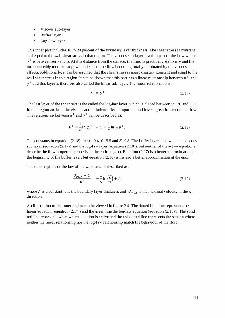
• Viscous sub-layer • Buffer layer

• Log -law layer

This inner part includes 10 to 20 percent of the boundary layer thickness. The shear stress is constant and equal to the wall shear stress in that region. The viscous sub-layer is a thin part of the flow where �� is between zero and 5. At this distance from the surface, the fluid is practically stationary and the turbulent eddy motions stop, which leads to the flow becoming totally dominated by the viscous effects. Additionally, it can be assumed that the shear stress is approximately constant and equal to the wall shear stress in this region. It can be shown that this part has a linear relationship between �� and �� and this layer is therefore also called the linear sub-layer. The linear relationship is:

�� = �� (2.17) The last layer of the inner part is the called the log-law layer, which is placed between �� 30 and 500. In this region are both the viscous and turbulent effects important and have a great impact on the flow. The relationship between �� and �� can be described as:

�� =1; ln(y�) + =

1; ln(<��) (2.18)

The constants in equation (2.18) are: ;=0.4, =5.5 and <=9.8. The buffer layer is between the viscous sub layer (equation (2.17)) and the log-law layer (equation (2.18)), but neither of these two equations describe the flow properties properly in the entire region. Equation (2.17) is a better approximation at the beginning of the buffer layer, but equation (2.18) is instead a better approximation at the end.

The outer regions or the law of the wake area is described as: �� − ��∗ = −1; ln =y

δ> + (2.19)

where is a constant, δ is the boundary layer thickness and �� is the maximal velocity in the x-direction. An illustration of the inner region can be viewed in figure 2.4. The dotted blue line represents the linear equation (equation (2.17)) and the green line the log-law equation (equation (2.18)). The solid red line represents when which equation is active and the red dotted line represents the section where neither the linear relationship nor the log-law relationship match the behaviour of the fluid.

12

Figure 2.4: The law of the wall formulation is shown in the figure. Red line indicates which law is used when. The blue and the green dotted lines indicate the extention of the linear relationship and log-law relationship, respectively. The red dotted lines represent sections where neighter of these relationships describe the behaviour of the fluid. �� is mainly used as a measure of how well resolved the solution is in near the wall region. Generally, a �� less than one deems a totally resolved boundary layer. If �� is larger than one, the boundary layer is not totally resolved and in those cases, so called wall functions are used to model the solution for the elements closest to the surface. To achieve a low ��, the grid has to be very fine, however finer grid often goes hand in hand with longer simulation times. Even though a low �� is desirable, different solution methods have different requirements and tolerances for high values on ��. Furthermore, areas of �� where the law of the wall does not describe the flow properly, as in the buffer layer and the outer layer, should be avoided when using traditional wall functions. Some softwares, such as Ansys Fluent’s �-equation based solvers use, as default, a wall treatment that is independent of ��, so special care of choosing �� is not needed to be taken into account [13].

2.3 RANS To solve the flow equations in their original form, as they are presented in equation (2.1) and equation (2.6-8), set high demands on the computations, which require high resolution both in time and space to capture the dynamic of the flow, which lead to very computationally heavy calculations. To get around this problem several simulation models have been developed, for example RANS, SAS and LES, that simplify the equations by modelling parts of the turbulent flow instead of computing all of it in the entire domain. Thereby the simulation time is shortened and is more or less dependent on how much of the turbulence is modelled and how much is resolved. The different models perform different simplifications, the RANS model models all structures and LES models only the small ones, which lead to differences in the results, simulation time, but also requirements of the time step and element size. The method that simplifies the flow more is not that time consuming as the one that computes the flow with fewer approximations, but can instead give a less good prediction of the flow. From an

13

engineering perspective, a model that is accurate and has low time consumption is favourable since time is money. As mentioned before, all models have more or less simplifications, these simplifications make the use of some algebraic equations necessary so the solution can be solved in an iterative way which will be described later in section 2.6.

The most used model, especially for engineering computations since it is the least expensive method, is the Reynolds Averaged Navier-Stokes (RANS) model. It is usually not that time consuming as other models, but not always that accurate. The main reason for why RANS has been the most used model is because it can run steady-state simulations. The solution of a RANS simulation will show how the turbulence affect the mean flow properties and not the instantaneous turbulent effects since it uses the simplification of performing calculations on the mean flow properties [2]. When one refers to the RANS equations for unsteady computations, it is the Unsteady Reynolds Averaged Navier-Stokes (URANS) equations that are meant. In the steady-state RANS equations, the time derivatives are zero in all the governing equations. In this study only transient simulations were performed, so when referring to RANS is it implicitly URANS.

The base for the RANS model is to rewrite the velocities and the pressure by use of the Reynolds decomposition (equation (2.10)) and then insert it into the Navier-Stokes equations and the continuity equation (equation (2.1), (2.6-8)). After that, a time-average of each of the four equations is computed, where the time-average part is calculated as in equation (2.11) and the time-average of the fluctuating part is calculated as:

8′? =1

∆� 9 8′&�'!� ≡ 0∆�

�

(2.20)

After some rewriting one gets the RANS equations for unsteady simulations:

!%�@ = 0 (2.21)

+�+� + !%�&�@' = −1�+A+" + �!%�,345!&�'-

+1� B+ /=−��′�CCCC>0+" +

+=&−��′�′CCCCC'>+� ++&−��′�′CCCCC'+$ D (2.22)

+E+� + !%�&E@' = −1�+A+� + �!%�,345!&E'-

+1� B+=&−��′�′CCCCC'>+" +

+ /=−��′�CCCC>0+� ++&−��′�′CCCCC'+$ D (2.23)

14

+F+� + !%�&F@'= −

1�+A+$ + �!%�,345!&F'-+

1� G+=&−��′�′CCCCC'>+" ++=&−��′�′CCCCC'>+� +

+ =−��′�CCCC>+$ H (2.24)

where �, E, F and A are time-averaged velocities and pressure, respectively. It can seem strange to use time-averages in transient equations, but the assumption that is used in the RANS equations is to use a much smaller time scale for the modelled fluctuations than for the resolved ones to make the results more transient-like. The time-averaging time scale used in equation (2.11) and (2.20) should be much smaller than the time step used in the simulations to give good results.

When the Reynolds decomposition (equation (2.10)) and the time-averaging is introduced into the Navier-Stokes equations, six additional terms are added in the RANS equations (2.22, 2.23 and 2.24), compared to the original Navier-Stokes equations (2.6-8). The normal and shear stresses in equation (2.25) and (2.26) are called the Reynolds stresses. The normal stresses are always non-zero.

* = −��′�CCCCCC*�� = −��′�CCCCCC*�� = −��′�CCCCCC (2.25) *� = *� = −��′�′CCCCCCC*� = *� = −��′�′CCCCCCC*�� = *�� = −��′�′CCCCCCC (2.26)

The specific Reynolds stress tensor can be written as:

*�� = −��′��′CCCCCCC (2.27)

where % and I are ", � or $. These stresses could not be computed directly since they are unknown, so they are modelled instead, by the use of a turbulence model that makes a prediction of the Reynolds stresses by use of the Boussinesq assumption that looks like:

−��′��′�CCCCCCC = �� J+��+"� ++��+"�K −

2

3��#�� = 2�� −

2

3��#�� (2.28)

where �� is the rates of deformation tensor, which is defined as:

�� =1

2J+��+"� +

+��+"�K (2.29)

By introducing the Boussinesq assumption, the six Reynolds stresses are approximated by the eddy viscosity, ��, which leads to a drastic simplification of the flow [2].

The models that will be described further on are the �-� and �-� models, and a combination of those two which is called the Shear Stress Transport (SST) model. These three turbulence models are so called two-equation models, meaning that besides the continuity and Navier-Stokes equations, they have two additional equations, so called transport equations that were described in equation (2.9). One of these additional transport equations, which is included in both RANS and SAS is the transport of turbulent kinetic energy �. The turbulent kinetic energy is defined by the modelled velocity fluctuations �′,�′ and �′ (same as in the Reynolds decomposition in equation (2.10)), which are the normal Reynolds stresses:

15

� =1

2�′��′�CCCCCCC =

1

2(�′�CCCC + �′�CCCC + �′�CCCCC) (2.30)

The transport equation for the kinetic energy can then be derived from the Navier-Stokes equations and looks like: +(��)+� + !%�&��@'

= !%� /−�′�′CCCCC+ 2��′L′��CCCCCCC− � 1

2�′�.�′��′�CCCCCCCCCCC0− 2�L′��. L′��CCCCCCCCC

− ��′��′�CCCCCCC.�� (2.31)

The second transport equation in the models transport different properties in the different models and will be described further on.

2.3.1 k-ε The �-� model is the most commonly used two-equation model, which originally was developed by Launder and Spalding in 1974 [1], since then many improvements have been added. It has one transport equation for the turbulent kinetic energy, �, and one for the rate of dissipation of turbulent kinetic energy, �, which is defined as:

� = 2�L′��. L′��CCCCCCCCCC (2.32)

As mentioned earlier, turbulent flow can be visualized as rotational structures by turbulent eddies, in addition to the fact that the eddies have different length scales, they also have different time scales. In an attempt to define the characteristics for these eddies they have been assigned a characteristic length ℓand the characteristic velocity M, which are used to define the turbulent viscosity ��. For the �-� model are they defined as:

M = √� (2.33)

ℓ =��/�� (2.34)

The turbulent viscosity, which also could be called the eddy viscosity, is computed for this turbulence model as: �� = ��Mℓ = � � �� (2.35)

where � is a dimensionless constant. The turbulent viscosity can be described as a regulator of the

turbulence in the flow in the RANS equations. High �� means that there is a lot of turbulence in the flow and that the fluid mixes well, whilst a low �� means low turbulence content and does not mix the fluid well.

In the definition of the turbulent viscosity is it assumed that it is isotropic, which is the same as that the components of the rate of deformation tensor are equal in all directions, which can lead to errors in complex flows and the use of another simulation models may be preferred.

The transport equation for � in the �-� model is derived from the exact transport equation for � (equation (2.31)) and is simplified by introducing the Boussinesq assumption (equation (2.28)) and

16

assuming that the turbulent diffusion transports � from locations where � is large to locations where � is small, since it wants to level out the differences in the flow to reach equilibrium. The transport equation for � is setup to look like the transport equation for �[2]. The two transport equations that are used in the �-� model look like: +(��)+� + !%�&��@' = !%� O��P� 345!�Q+ 2�� . �� − �� (2.36)

+(��)+� + !%�&��@' = !%� O��P� 345!�Q + �� 2�� . �� − �� (2.37)

where the constants in equation (2.36) and equation (2.37), for a standard �-� are [1]:

� = 0.09P� = 1.00P� = 1.30 �� = 1.44 �� = 1.92

�, ��, and �� are dimensionless modelling constants that have been determined by validating

experiments with simulated results. P� and P� are the Prandtl numbers for � and �, respectively, which gives information about the diffusivity of � and �, respectively. The terms in the transport equation (2.36), which are valid for all transport equations, are describing the rate of change, transport by convection, transport by diffusion, rate of production and rate of destruction of �, respectively. The same information is given from each term in equation (2.37) but for � instead. The transport equations for � and � (equation (2.36-37)) are then used as a coupling for solving the RANS equations (equation (2.21-24)).

The �-� model is very good at predicting confined flows and computing the flow in the free stream which covers many engineering applications, hence its popularity. On the other hand the �-� model do not give any good predictions of unconfined flows and with weak shear layers. Adverse pressure gradients are also problematic because the model has low dissipation which produces a too large length scale which leads to that it over-predicts the shear stresses in that regions [2].

2.3.2 k-ω The �-� model, often called the Wilcox-�-� and originated in 1988, named after its inventor, is another turbulence model that is used in RANS simulations. The difference between the �-� and the �-� model is that the second transport equation for � is replaced by a transport equation for the specific dissipation �, which is defined as:

� = � �⁄ (2.38) The characteristic velocity looks the same as in equation (2.33) for the �-� model, but the characteristic length is instead computed as:

ℓ =√�� (2.39)

which leads to the following eddy viscosity:

�� = �Mℓ =�� (2.40)

17

The transport equation for � is a little bit different due to the change from � to � and looks like: +(��)+� + !%�&��@' = !%� O/� +

��P�0345!&�'Q + A� − R∗�� (2.41)

where

A� = 2�� . �� −2

3�� +��+"� #�� (2.42)

The transport equation for � looks like: +(��)+� + !%�&��@'

= !%� O/� +��P�0 345!&�'Q+ S� J2�� . �� −

2

3��+��+"� #��K

− R�� (2.43)

The model constants are the following [1]:

P� = 2.0P� = 2.0S� = 0.553R� = 0.075R∗ = 0.09

In the same way as for the �-� model, the � and � equations are used as a coupling for solving the RANS equations (equation (2.21-24)). The Reynolds stresses are computed in the same way as for the �-� model, by use of the Boussinesq assumption (2.28) and are implemented into the RANS equations.

In the free stream flow, where � and � goes to zero, this model have some problems with the prediction of the flow. The reason for this is because equation (2.43) goes to infinity or becomes indeterminate for these values, which is solved by giving � a lowest possible value. The downside of this is that in flows where � is important, for example in external aerodynamic applications, the accuracy of the predictions are highly based on the guessed minimal value [2]. The advantage of this model is that the predictions of the near-wall regions are good because it includes the molecular viscosity in the transport equations for � and � (equation (2.41 and 2.43)) which is dominant in the boundary layer. In comparison with the �-� equations (equation (2.36-37)), only the turbulent viscosity is included and gives no information about the molecular viscosity. In the bulk flow where the flow is turbulent, the turbulent viscosity is dominant and therefore produces good results in the free stream flow.

2.3.3 SST The SST model (Shear Stress Transport), often also called the Menter SST �-� model, which has been invented by Florian Menter in 1992, is a combination of the �-� and the �-� model that have been described in section 2.3.1 and 2.3.2. The idea of this model is that the �-� model is good at predicting the flow in the free stream and the �-� model is good at predicting the wall shear stresses close to the boundaries. The advantage of the SST model is that it transforms the �-� equations into the �-� equations in the near-wall regions. The �-equation is the same as in the �-� model, namely: +(��)+� + !%�&��@' = !%� O/� +

��P�0345!&�'Q + A� − R∗�� (2.44)

18

The �-equation, equation (2.37), is transformed to a �-equation by replacing � by � = ��, which gives the following transport equation for �: +&��'+� + !%�&��@'

= !%� TJ� +��P�,�

K345!&�'U + S� J2�� . �� −2

3�� +��+"� #��K

− R�� + 2�P�,�

+�+"� +�+"�

(2.45)

where the model constants are [1]:

P� = 2.0P�,� = 2.0P�,� = 1.17S� = 0.44R� = 0.08R∗ = 0.09

The procedure for solving the RANS equations is the same as for the �-� and �-� model which was described earlier.

By comparing equation (2.43) with equation (2.45) there is an extra term on the right hand side (the last term in equation (2.45)), which has arisen due to the transformation from the �-equation to the �-equation.

To be able to switch from the �-� to �-�, the SST model uses so called blending functions. Both the standard �-� and the transformed �-� equations are multiplied by a blending function and then added together. A blending function is constructed in such a way that it is zero far away from walls, which activates the �-� model, and one close to the boundaries which activates the �-� model instead. It makes a smooth transition between the two models at the middle of the boundary layer. This approach makes the SST model robust and reduces the influence of numerical instabilities. Since this turbulence model is a combination of two models that are good at different things in different situations it makes the SST model applicable for many flow situations [13]. Furthermore a limitation of the eddy viscosity is implemented to make the model’s prediction of the flow better in flows with adverse pressure gradients and wakes. The eddy viscosity then looks like:

�� =5��V5"&5��, ��' (2.46)

where � = W2�� . ��, 5� is a constant and �� is a blending function.

A limitation of the production of turbulent kinetic energy is also used to avoid too high production of turbulence at locations with zero velocity and looks like:

A� = V%X J10R∗��, 2�� . �� −2

3�� +��+"� #��K (2.47)

2.4 LES As stated earlier, large and small eddies have different kinetic energies. When using a RANS model, all of the eddies are modelled with the same turbulence model, for example the �-� or the �-� model, for solving the whole flow, which can have large variations in the size and energy of the eddies that could be difficult to compute. Another approach could be used for solving the Navier-Stokes equations, namely the Large Eddy Simulation (LES) method. It separates the small scales from the

19

large, and resolves the large ones only. The smallest eddies are modelled with the assumption that they appear where shear stresses occur, such as close to walls or in wakes, that make them almost non-directional and therefore assumed to be isotropic and can be modelled with a satisfactory precision. The larger eddies appear in for example wakes, where the turbulence is high which make the eddies strongly three dimensional and anisotropic, and almost all of the Reynolds stresses are transported by them. Furthermore, they are strongly affected by the used boundary conditions and therefore need to be resolved [3]. By only resolving the large eddies, it is allowed to use a coarser grid compared to Direct Numerical Simulations (DNS) method where all eddies are resolved, but also a larger time-step could be used for resolving the flow field accurate enough.

LES uses a spatial filter to separate the large and small eddies, instead of using the time-averaging approach as in the RANS models. The filter is constructed in such a way, so that the eddies that are smaller than the filter size (cutoff width), �, are modelled and the larger ones are resolved. The information regarding the larger eddies is saved and the smaller eddies, so called subgrid scales (SGS),

are instead modelled by a SGS-model. In LES is the filtered function 6Y&(' defined as [13]:

6Y&(' = 9 Z,(, (′-6((′)!(′�

(2.48)

where � is the fluid domain, Z,(,(′- is the spatial filter function and 6((′) the unfiltered function.

Since ANSYS Fluent uses a finite-volume discretization, the filtering function looks like:

Z,(,(′- = [1 E� , " ′ ∈ �0, " ′\�ℎ�4�%L�] (2.49)

which produces the following filtered function 6Y&(': 6Y&(' =

1E9 6((′)!(′�

, " ′ ∈ � (2.50)

In three dimensional computations in Fluent the cutoff width is often taken to be the cubic root of the element sizes in each direction as:

� = W�"��$� (2.51)

The cutoff width is a limit of the resolution of the computations, since it determines the size of the smallest scales that will be resolved. Eddies smaller than the cutoff width will be modelled by the SGS-model and the larger ones will be resolved.

The filtering procedure leads to the fact that the variables in the LES equations are functions of both time and space. The LES equations are obtained by first using the filtering function, described by equation (2.50), on the velocities and the pressure, and afterwards inserting them into the Navier-Stokes equations (equations (2.1) and (2.6-8)). After some rewriting one get the governing equations for an LES computation:

!%�&�̂' = 0 (2.52) +&�_'+� + !%�&�_�̂' = −

1�+�_+" + �!%�,345!&�_'- − ,!%�&��̀' − !%�&�_�̂'- (2.53) +&�_'+� + !%�&�_�̂' = −1�+�_+� + �!%�,345!&�_'- − ,!%�&��̀' − !%�&�_�̂'- (2.54)

20

+&�̂'+� + !%�&�̂�̂' = −1�+�_+$ + �!%�,345!&�̂'- − ,!%�&��̀' − !%�&��̂'- (2.55)

The last parenthesis in equations (2.53-55) develops due to the filtering operation, similar to the Reynolds stresses that develop when deriving the RANS equations. These two terms in the x-direction (equation (2.53)) could be rewritten as:

!%�&��̀' − !%�&�_�̂' =+&��̀ − ��̂�_'+" +

+&��̀ − ��̂�_'+� ++&��̀ − ��̂�'+$ =

+*��+"� (2.56) *�� is the so called Sub-Grid-Scale (SGS) stress, which could be rewritten on the following form:

*�� = ��` − ��̂��̂ = ,��̂��̂a − ��̂��̂-bccccdcccce�

+ ,��̂��a + ��̂a -bccccdcccce�

+ ��abde�

(2.57)

The SGS stresses could be divided into three parts:

1. Leonard stresses �� 2. Cross-stresses �� 3. LES Reynolds stresses ��

The Leonard stresses are due to effects of the resolved scale, the cross stresses models the interaction between the resolved flow and the SGS eddies, and the LES stresses develop due to the interactions of the SGS eddies because of the convective momentum transfer. The SGS stresses are those that have to be modelled by a SGS turbulence model [1]. As in the RANS model, Fluent uses the Boussinesq assumption (equation (2.28)) to calculate the SGS turbulent stresses in equation (2.57) as [13]:

*�� −1

3*��#�� = −2�� ̅�� (2.58)

where �� is the SubGrid-Scale turbulent viscosity, which is defined in different ways depending on the SGS model. *�� is the isotropic part of the SGS stresses, which is not modelled, but added to the static pressure term. �̅�� is the rate-of-strain tensor for the resolved scale and is similar to the one in

equation (2.29):

�̅�� =1

2J+�C�+"� +

+�C�+"�K (2.59)

The SGS stresses defined in equation (2.57) can also be written in the following form:

*�� −1

3*��#��bcccdccce

�!��"��

+1

3*��#��bcdce

�#"��"$��

(2.60)

The deviatoric part of the SGS stress tensor can be modelled as:

*�� −1

3*��#�� = −2�� /�� −

1

3��#��0 (2.61)

To compute �� , a SGS model is used. In this thesis the Wall-Adaptive Local Eddy-Viscosity (WALE) model was used, which computes �� as [13]:

21

�� = �� ,��-�/�,�̅��̅��-%/� + ,��-%/& (2.62)

where �# is the mixing length for subgrid scales. �# and �� are defined as:

�# = V%X&;!, '∆' (2.63)

�� =1

2,3̅�� + 3̅�� - −

1

3#��3̅�� (2.64)

3̅�� =+�C�+"� (2.65)

where ; is the von Kárman constant, ! is the distance to the closest wall and � is the local grid scale and is calculated as in equation (2.51). The WALE constant ' is 0.325, which is a default setting in ANSYS Fluent [14]. The WALE model is preferable because it works well for flows in regions where transition from laminar to turbulent flow occurs. It produces a �� which is zero where pure shear occurs in laminar regions, which is physically correct since the roughness of the wall dampens out all turbulent fluctuations, which other models like the Lilly-Smagorinsky model does not do, without an introduction of a damping function [19]. This makes this model to perform well in transition regions.

It is important to use a spatial and time discretization scheme that is non-dissipative, like Central Differencing, since the SGS model produces a dissipation of the turbulence itself. If a dissipative discretization scheme, like Upwind is used, there would be too much dissipation in the solution that would dampen out too much of the turbulence in the flow [2].

The LES model works better for many flow cases for which the RANS model has problems, such as flows with large separation, transition regions but also flows around bluff-bodies, since large turbulent structures occur in the wake that are time dependent [2]. The disadvantage with LES is that it normally needs a finer mesh than RANS to compute accurate results, and also by resolving a larger part of the flow contributes to the extended computational time since a smaller time step is needed to make a good time resolution of the computations. Furthermore, it needs to be run for a longer time to get stable statistics from the computations. [2, 3, 13]

2.5 Hybrid models In some instances the RANS model is not accurate enough but LES is too expensive for many industrial engineering problems. Therefore hybrid models which include both RANS and LES qualities, have been developed to make the computations less expensive than for the LES model, but with better accuracy than the RANS model. These hybrids use the RANS model in flows where the eddies are small and could be computed with good accuracy by the RANS model. In the free stream flow, where the large eddies dominate the flow characteristics, the hybrid model will switch to LES mode instead. There are several different hybrid models that perform this switch of simulation models in different ways. One of these models is the Scale Adaptive Simulation (SAS) model, which switches from RANS to a LES-like solver depending on the length scales of the eddies and the element size. This model is the one that will be investigated thoroughly in this thesis work.

22

2.5.1 SAS The SAS model’s main purpose is to improve the RANS models ability to compute large scale motions in the free stream flow. In these turbulent areas, the SAS model has a LES-like behaviour with the advantage that it can return from LES mode to RANS mode again if the grid size or time step does not meet the requirements to run the simulation in LES mode. This makes the SAS simulation model much more robust compared to other hybrid models. The concept of the SAS model is to introduce the von Karman length-scale, ��, into the SST transport equation for � (equation 2.45) to detect unsteadiness in the flow. When unsteadiness is detected, the aim is to lower the eddy viscosity so that the fluctuations in the flow will not be dampened out and destroyed, but instead be resolved by the LES like part of the simulation model.

The SAS model that will be investigated is the SAS-SST model which could be explained as the RANS-SST model with LES features. As in the RANS-SST model, the SAS-SST model uses a transport equation for the turbulent kinetic energy, �, and one for the vorticity, �. In ANSYS Fluent the SAS-SST model is based on the Rotta’s �-� (SST) approach, which represents the large scales of the turbulence and the transport equations look like: +��+� +

++"� &��' = Z� − �g�� +++"� T/� +

��P�0 +�+"�U (2.66)

+��+� +++"� &��' = h�� Z� − �R�� + i�(� +

++"� T/� +��P�0 +�+"�U +

(1 − ��)2�P�,�

1� +�+"� +�+"� (2.67)

where Z� = −�� +��+"� (2.68)

P�,� = P� when the SST-model is in the �-� mode.These two transport equations are similar to the

transport equations for the RANS-SST model (equation (2.44-45)), but in the �-equation an extra source term is added, i�(�, for the turbulent frequency. It originates from the second derivative term in the Rotta’s transport equation which is a more exact transport equation of � and looks like [13]:

i�(� = V5" T�j�;�� / ��0� − ∙2��P) V5" J 1��

+�+"� +�+"� ,1�� +�+"� +�+"�K , 0U (2.69)

where j� = 3.51 , P) = 2/3, = 2 and � is the modelled turbulent length scale, which is defined as:

� = √�/ =g��/& ∙ �> (2.70)

The von Kármán length scale in three dimensions is defined as:

��,�� = ; �|�′′| (2.71)

where |�′′| is defined as [13]:

23

l�′′l = mnJ +��+"�+"�K�(�)

(2.72)

The model includes a direct control of the high wave number damping and is done by a lower constraint on the von Kármán length scale as:

�� = V5"o; �|�′′| , �: ;j�,R/g�- − h ∙ Δp (2.73)

The purpose of the i�(� -term is to increase the turbulent frequency � when the von Kármán length scale �� is low, which will lower the turbulent viscosity and counteracting the damping of the turbulence in the flow [2].

When the flow is steady, the SAS model performs computations in RANS mode which should lead to faster calculations since it does not require such a fine grid as LES. When the flow becomes unsteady, �� will decrease, which in turn leads to a decrease of the eddy viscosity in the flow. This is desirable since a high eddy viscosity will dampen out a large amount of the created turbulence which one wants to resolve. When the unsteadiness in the flow field is not high enough, the SAS model will not switch into the LES mode but instead stay in the RANS mode. This could be considered to be good since the worst thing that will happen is that the accuracy will be worse than expected. On the other hand, if it does not switch into LES mode, the turbulence will be dampened out and finally destroyed due to the high eddy viscosity that RANS produces and therefore stay in the RANS mode throughout the simulation. The main advantage of the SAS-SST model is that when it performs computations in the RANS mode the solution is independent of the element size and therefore the accuracy will not be affected when the unsteadiness is low [13,14].

2.6 Pressure-velocity coupling Each simulation model, as RANS, SAS and LES, has to use a pressure-velocity coupling to give information about the pressure to the flow equations to make it possible to compute the velocities in the flow equations. For compressible and heat transfer calculations, the energy equation is used together with the ideal gas law to compute the pressure, which is then used for solving the Navier-Stokes equations (equations (2.1, 2.6, 2.7 and 2.8)). For incompressible and isothermal computations, the density and the temperature are constant, so these equations do not give any information about the pressure that is used for solving the Navier-Stokes equations as mentioned before. For the incompressible computations, the pressure is computed in an iterative way instead of using the energy equation and the gas law or any other equations, by the use of for example the SIMPLEC (Semi-Implicit Method for Pressure-Linked Equations-Consistent) algorithm. It starts by an initial guess of the pressure �∗ that is used in the momentum equations to obtain the velocity components for the guessed pressure values �∗, �∗ and �∗. These guessed values will lead to an error, �′, between the correct pressure, �, due the pressure computed from the guessed value, �∗, and is computed as:

�� = � − �∗ (2.74)

The corrected pressure � is then inserted into the momentum equations from which the correct velocities �, � and � are computed. By repeating this procedure in the next iteration, but instead taking the difference between the pressure computed in the current iteration, �, and the pressure

24

computed in the iteration before, �∗, the error becomes smaller. This procedure is repeated until it reaches a chosen convergence criterion. To get away from divergence, which can be obtained by adding too much of the correction term ��, under-relaxation is used, so equation (2.74) will instead look like:

� = �∗ + h$�� (2.75)

where h$ is the under-relaxation factor for the pressure which is between zero and one to obtain

under-relaxation. A low h$ leads to more stable computations but usually needs more sub-iteration to

reach convergence. On the other hand, a high h$ could lead to divergence of the results, so an optimal

value has to be found for the current flow situation. For the velocity there is also under-relaxation used, which for the �-component looks like:

�*!' = h+�(*) + &1 − h+'�(*,�) (2.76)

where h+ is the under-relaxation term for the �-velocity, �(*) is the corrected velocity obtained in the

current iteration and �(*,�) is the corrected velocity obtained in the previous iteration. The SIMPLEC method is preferable because it often allows higher under-relaxation terms than for the SIMPLE method on which SIMPLEC is based. The difference between these two methods is that SIMPLEC omits terms that are less significant in the correction equation, which yields to faster calculations due to the higher under-relaxation factor [13, 14].

25

3. Method To determine the how accurate the SAS-model is, the two test cases that were described earlier were run on three and two different mesh structures, respectively. For the first test case, simulations with RANS, SAS and LES were performed, but for the second case only SAS simulations were performed. The simulation results were validated by comparing them with experimental measurements. The first test case was used to get a deeper understanding of the different simulation methods and their grid dependency. The different mesh structures that were analyzed for the first test case was; unstructured tetrahedral, structured hexahedral and unstructured polyhedral. For the second test case only the structured hexahedral and the unstructured polyhedral mesh types were analyzed. For the meshes in test case 1, different grid sizes for the elements in an area close to the cylinder were investigated to get a better understanding of how the results were affected by the element size. No further mesh dependence study was made, apart from the eight different tested meshes, as this is in accordance with normal simulation procedures in the industry. The findings from this study were then used for the other test case that was used for validation of the conclusions drawn from the first test case to see if they were applicable on another flow situation.

The investigation of the simulation models also covered their computational cost of the simulations. The time for calculating 100 iterations and the number of used CPU’s for each calculation was noted and compared with each other.

All simulations were made in ANSYS Fluent version 14.0. Post-processing was done in ANSYS Fluent v.14.5, ANSYS CFD Post v.14.5, Paraview v.3.98.0 and Matlab R2008a. These softwares were used since FS Dynamics use them for their computations and wanted to get results that were as similar as possible to their standard computations. Furthermore, ANSYS Fluent is often preferred because it has a good solver that is stable and robust.

The simulations were run at different computers and clusters, namely:

• Stockholm cluster, FS Dynamics • Gothenburg cluster, FS Dynamics • National Supercomputer Centre (NSC), Linköping University

• Local computers in Stockholm, FS Dynamics

The local computers were run either on a single computer or by connecting several local computers for generating a cluster.

3.1 Case 1 – Cylinder The first test case was a wall-mounted vertical cylinder in a wind tunnel test section (figure 3.1). The flow situation that was wanted to mimic was the measurements reported in the papers of Sumner et al. [7, 8, 9, 10]. The measurements were executed in a low-speed wind tunnel of flow past cylinders with different , from three to nine. nine was chosen as test case 1, because of the uncertainties of the vortices in the flow for lower as stated in section 1.2.1. The domain size and cylinder location was chosen to be the same as in the experiments and are shown in figure 3.1. In the experiments a tip wire was used at the beginning of the test section to increase the turbulence in the flow which was excluded in the simulations. Instead, the domain started at the location of the tip wire. The cylinder had a diameter of 31.5 mm, the free stream velocity, �∞, was 20 m/s that corresponded to a Reynolds number of 42,000. Because of the low free stream velocity, which corresponded to a Mach number of 0.06, which is below 0.1 that could be used as a rule of thumb for when the air could be treated as an

26

incompressible fluid, provided that no large pressure variations occur according to Fluent [14]. The used air density for the computations was 1.225 kg/m3 and the dynamic viscosity was 18.37∙10-6 Pa s, based on a temperature of 15 degrees and a pressure of 1 atm. For almost all simulations the turbulence intensity at the inlet was set to 0.6 percent, which was the measured free stream turbulence intensity in the experiments and the turbulent viscosity ratio was set to 10. There was an exception for two test cases named low respectively high turbulence intensity (LTI and HTI cases) where the turbulence intensity was set to 0.1 and 3 percent, and the turbulent viscosity ratio was set to 1 and 100 respectively. This was done for investigating the impact of the turbulence in the flow on the SAS model. The idea of using low turbulence intensity was to decrease the turbulence in the flow and thereby make the flow to separate earlier to get a higher drag coefficient. The idea of trying higher turbulence intensity was to force the SAS model to perform a larger part of the flow field in the LES mode. In addition to these two extra simulations, another three simulations were run with RANS, SAS and LES on the coarsest structured mesh where �� was lowered below one on the cylinder surface, which was done to investigate the �� dependency. For RANS and SAS this means an exclusion of using wall functions in the computations and in LES it leads to that smaller structures are resolved due to a decreased cutoff width.

The inlet wall of the domain (figure 3.1) was set to a velocity-inlet boundary condition in Fluent. To resemble the same flow conditions as in the experiments, a fully developed velocity profile was applied on the inlet surface and the profile had a specified �-velocity over the height (z-direction), which was read from a text file, and the �- and �-velocities were set to zero. The velocity profile with the free stream velocity 20 m/s (Reynolds number 42,000) was measured at the location of the cylinder, but with the cylinder removed. In the LES model, a spectral synthesizer was used on the inlet

D

H= 9.00D

17.75 D

22.22 D

62.20 D

35.90 D

28.90 D

�∞

y x

z

INLET

OUTLET

Figure 3.1: Geometry of test case 1 with its dimensions (D= 31.5 mm). U∞ was 20 m/s to simulate Re� 42,000. The origin of

the coordinate system was positioned at the centre of the cylinder as shown in the figure.

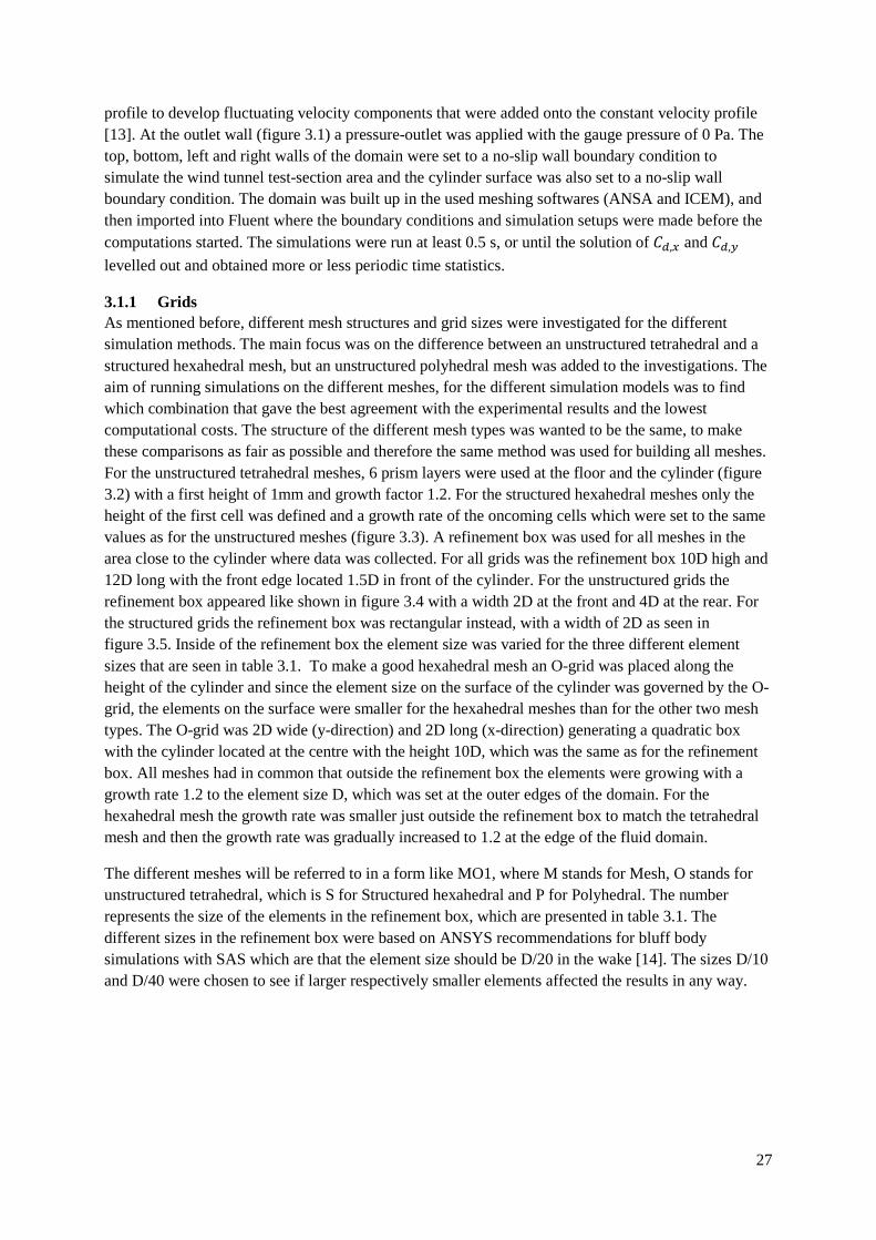
27

profile to develop fluctuating velocity components that were added onto the constant velocity profile [13]. At the outlet wall (figure 3.1) a pressure-outlet was applied with the gauge pressure of 0 Pa. The top, bottom, left and right walls of the domain were set to a no-slip wall boundary condition to simulate the wind tunnel test-section area and the cylinder surface was also set to a no-slip wall boundary condition. The domain was built up in the used meshing softwares (ANSA and ICEM), and then imported into Fluent where the boundary conditions and simulation setups were made before the computations started. The simulations were run at least 0.5 s, or until the solution of �, and �,�

levelled out and obtained more or less periodic time statistics.

3.1.1 Grids As mentioned before, different mesh structures and grid sizes were investigated for the different simulation methods. The main focus was on the difference between an unstructured tetrahedral and a structured hexahedral mesh, but an unstructured polyhedral mesh was added to the investigations. The aim of running simulations on the different meshes, for the different simulation models was to find which combination that gave the best agreement with the experimental results and the lowest computational costs. The structure of the different mesh types was wanted to be the same, to make these comparisons as fair as possible and therefore the same method was used for building all meshes. For the unstructured tetrahedral meshes, 6 prism layers were used at the floor and the cylinder (figure 3.2) with a first height of 1mm and growth factor 1.2. For the structured hexahedral meshes only the height of the first cell was defined and a growth rate of the oncoming cells which were set to the same values as for the unstructured meshes (figure 3.3). A refinement box was used for all meshes in the area close to the cylinder where data was collected. For all grids was the refinement box 10D high and 12D long with the front edge located 1.5D in front of the cylinder. For the unstructured grids the refinement box appeared like shown in figure 3.4 with a width 2D at the front and 4D at the rear. For the structured grids the refinement box was rectangular instead, with a width of 2D as seen in figure 3.5. Inside of the refinement box the element size was varied for the three different element sizes that are seen in table 3.1. To make a good hexahedral mesh an O-grid was placed along the height of the cylinder and since the element size on the surface of the cylinder was governed by the O-grid, the elements on the surface were smaller for the hexahedral meshes than for the other two mesh types. The O-grid was 2D wide (y-direction) and 2D long (x-direction) generating a quadratic box with the cylinder located at the centre with the height 10D, which was the same as for the refinement box. All meshes had in common that outside the refinement box the elements were growing with a growth rate 1.2 to the element size D, which was set at the outer edges of the domain. For the hexahedral mesh the growth rate was smaller just outside the refinement box to match the tetrahedral mesh and then the growth rate was gradually increased to 1.2 at the edge of the fluid domain.

The different meshes will be referred to in a form like MO1, where M stands for Mesh, O stands for unstructured tetrahedral, which is S for Structured hexahedral and P for Polyhedral. The number represents the size of the elements in the refinement box, which are presented in table 3.1. The different sizes in the refinement box were based on ANSYS recommendations for bluff body simulations with SAS which are that the element size should be D/20 in the wake [14]. The sizes D/10 and D/40 were chosen to see if larger respectively smaller elements affected the results in any way.

28

Figure 3.2: The coarsest unstructured tetrahedral mesh (MO1), with the sizes as mesh number 1 in table 3.1.

Figure 3.3: The coarsest structured hexahedral mesh (MS1) with the sizes as mesh number 1 in table 3.1.

29

Figure 3.4: The coarsest unstructured tetrahedral mesh (MO1), top view, with the sizes as mesh number 1 in table 3.1. The blue box is the borders of the refinement box.

Figure 3.5: The coarsest structured hexahedral mesh (MS1), top view, with the sizes as mesh number 1 in table 3.1.

30

Table 3.1: Mesh study parameters that were varied during the investigation for the different mesh types. D=31.5mm.

Mesh study Mesh Size

Cylinder surface Refinement box Free stream box

1 D/10 D/10 D

2 D/20 D/20 D

3 D/40 D/40 D

For the tetrahedral and polyhedral grids, only the two coarsest element sizes were investigated because the finest one would have given too large meshes to perform computations on that would not be practicable. The tetrahedral meshes were done in ANSA 13.2.3 and the hexahedral meshes were done in ICEM R14.5. The polyhedral mesh was done by transforming an unstructured tetrahedral mesh into a polyhedral mesh in Fluent.

All the meshes that were simulated and with which simulation model, can be seen in table 3.2. The number of cells and �� for the different meshes can be found in table A.2 in appendix.

Table 3.2 An overview of all performed simulations in test case 1.

Performed simulations test case 1 Mesh RANS SAS LES MO1 X X X MO2 X X - MS1 X X X MS2 X X X MS3 X X - MP1 X X X MP2 - X -

MS1 y+<1 X X X MS1 HTI - X - MS1 LTI - X -

3.1.2 Time step The when selecting the time step the aim was to achieve a Courant- Friedrichs- Lewy (CFL) number equal to or lower than one in the refinement box to capture the dynamics of the flow. The ��-number is defined as:

�� =�∆�∆" ≤ 1 (3.1)

where � is the velocity, ∆" is the grid size and ∆� is the time step. The CFL-number can be used as a guide line for determining the size of the time step for resolving the flow properties as good as they can be on that specific grid. A smaller time step than required give longer simulation times, but no improvement of the solution if the element size is not decreased. Based on the cell size inside the

31

refinement box and the free stream velocity, the time step was chosen and guided by equation (3.1). The ��-number was verified by running simulations with the used time step shown in table 3.3.

Table 3.3: Used time steps for the different grid sizes.

Time step Mesh Size [s]

1 1∙10-4

2 5∙10-5 3 2.5∙10-5

3.1.3 Setup The pressure-velocity coupling method used for all simulations was SIMPLEC, since it usually allows higher under-relaxation terms than the SIMPLE method which leads to faster simulations. The used setups for the different simulation methods are presented in table 3.4, which are recommendations from ANSYS for running simulations with each simulation methods [4, 13, 14]. For the gradient evaluation, Least Squares Cell Based (LSCB) was used because it gives a better accuracy on non-orthogonal meshes, as tetrahedral and polyhedral meshes [4, 13], and also for meshes with skewed cells. For the pressure equation in the LES simulations “Standard” discretization was used for the reason of convergence problems when using the “Second Order” discretizaion scheme. The standard discretization scheme in Fluent is a co-located scheme which computes the pressure at cell centres. The Second Order Upwind scheme computes the pressure at the cell centre by interpolating the pressure at the two cell faces upstream from that cell, which is more accurate than the co-located scheme [13]. The reason for not using an upwind scheme for SAS, and instead using a central differencing scheme is because one does not want a highly dissipative discretization scheme, because it dampens the unsteadiness in the flow which would lead to it never switching into LES mode. For LES, a central differencing scheme was used because when using SGS-models it is undesirable to get more dissipation than what the SGS-model produces itself, as described in section 2.4. Bounded Central Differencing (BCD) was used for SAS because it is recommended by ANSYS [14] due to the use of both RANS and LES-like computations. In the LES simulations BCD was used for the reason that the Central Differencing (CD) scheme can lead to unphysical wiggles in complex flows, why BCD is recommended since it is a little bit more dissipative than the CD scheme and therefore dampens these wiggles. The second order discretization scheme was used to get better accuracy since the flow was fairly complex and that the flow was not aligned with the mesh, especially in the wake of the cylinder, which can lead to a reduction of accuracy if a first order discretization scheme is used [14].

32

Table 3.4: Used setup for SIMPLEC for the three different simulation methods.

Pressure-velocity coupling RANS SAS LES Discretization method SIMPLEC SIMPLEC SIMPLEC Gradient LSCB LSCB LSCB

Pressure 2nd Order 2nd Order Standard

Momentum 2nd Order Upwind BCD BCD

Turbulent Kinetic Energy 2nd Order Upwind 2nd Order Upwind -

Specific Dissipation Rate 2nd Order Upwind 2nd Order Upwind -

Transient formulation 2nd OI BSOI BSOI

BSOI= Bounded Second Order Implicit 2nd OI= Second Order Implicit LSCB= Least Squares Cell Based BCD= Bounded Central Differencing

The under-relaxation factors that have been used can be found in table A.1 in appendix.

The convergence criterion was set to relative, which means that the ratio between the residual of the current iteration at a time step and the residual of the iteration at the beginning of that time step is less than the defined value [14]. When the ratio reaches the user-defined value that was set to 0.05, the solution is converged for that time step. The maximum number of sub iterations was set to 20 for all simulations.

Almost all simulations were initialized from an almost converged SAS solution for MS2. MO1 RANS, MS1 SAS and MS2 SAS were initialized from a steady-state solution.

3.1.4 Post processing The drag coefficient, �, for the simulations was computed as a time-average over the last 0.4 s of the simulated time statistics of � that is defined as:

� =��

12��

(3.2)

where �� is the sum of the forces that are acting on the cylinder and is the reference area that is = � ∙ �. The time statistics for the last 0.4 s for all simulations had levelled out and had reached a periodic solution that was appropriate to use for time-averaging.

The Strouhal number gives information about the oscillations in the flow, in this case the vortex shedding that is acting on the cylinder, and is defined as:

�� =�� (3.3)

where � is the shedding frequency and � is the characteristic length that is the diameter, �, in this case. The shedding frequency was obtained by making a Fast Fourier Transform (FFT) of the monitored velocity magnitude at a point located at x=3D, y=1.5D and z=5D, which was the same position where data has been taken from to compute the Fourier spectra in the experiments performed by Sumner et al. [9] that were used for comparison.

33

To determine the separation angle the time-averaged wall shear stress in the x-direction on the cylinder was monitored. The x-position where the wall shear stress switched from positive to negative was calculated along the height of the cylinder by using the average x-position from which the separation angle, �, was calculated. A schematic picture of how the separation angle was defined can be seen in figure 3.6.

Figure 3.6: Definition of the separation angle. The oncoming flow comes from the left and the flow detaches from the cylinder at the separation point, with the separation angle �.

3.2 Case 2 – Aorta The second test case was an aorta with a coarctation in the descending aorta. The geometry for the specific aorta was obtained from MRI-measurements made at Linköping University Hospital. A simplified and smoothed CAD-model of the aorta was obtained from Linköping University. Only two branching vessels were included in the model to make the meshing and computations easier and these simplifications should not have affected the results in a large scale according to Lantz [15]. The walls were assumed to be rigid walls that were impermeable and fixed in space. In reality, the arterial walls are flexible and moves during the cardiac cycle, but this assumption should not lead to any large errors in the results [15]. The fluid was assumed to be incompressible and behave as a Newtonian fluid. Blood behaves normally as a non-Newtonian fluid, but for large blood vessels, as the aorta, where the diameter is larger than 1 mm and the shear rates are larger than 100 s-1, which holds for this case, it could be assumed to behave as a Newtonian fluid [15]. This could be further explained by the use of the Casson and Carreau-Yashuda models, that are used for describing the relationship between the viscosity and shear tinning for non-Newtonian fluids. For large shear rates and large diameters, the non-Newtonian viscosity approaches the Newtonian viscosity, why this assumption could be used without any large errors for the blood flow in the aorta [15]. The used molecular viscosity and density for the blood was 0.0035 Pa s and 1060 kg/m3, respectively.

Furthermore, the three velocity components in x-, y- and z-direction and the turbulent kinetic energy for the flow in the patient specific aorta was obtained for the whole aorta from the MRI-measurements. The mass flow rates at the ascending aortic inlet (Asc) and the two branching vessels; brachiocephalic (BCA) and left common carotid arteries (LCCA), see figure 3.7, for one cardiac cycle was obtained and were used as boundary conditions at these locations in the model. Due to the cardiac cycle, which was described in section 1.2.2, the simulated flow through the aorta is pulsating and was simulated by using time dependent boundary conditions from MRI-measurements at the ascending aortic inlet (Asc), brachiocephalic artery (BCA) and left common carotid arteries (LCCA). At the ascending aortic (Asc) inlet, the mass flow rate looked like in figure 3.8. The simulations were performed for eight cardiac cycles with equal boundary conditions for one phase-averaged pulse. The reason for running several cardiac cycles was to get a good phase-average of the results since the velocities and the turbulent kinetic energy from the MRI-measurements were phase-averaged over several cycles. The first cycle was not included when calculating the phase-average, since the first cycle was visibly different than the next oncoming cycles due to the affect of the initial condition, so only seven cycles were evaluated. At the outlet of the aorta, the boundary condition was set to a pressure outlet with the

Separation point

θ Oncoming flow

34

gauge pressure 0 Pa. The turbulence intensity at the inlet was set to 10 percent which seemed to be reasonable since the patient had a narrowed heart valve which produced a turbulent flow entering the aorta.

Several monitor points were positioned out through the aorta, especially in the neighbourhood of the coarctation where the blood flow became turbulent and was of interest for validating the SAS model’s performance. The points that data were collected from are seen in figure 3.7, where the used coordinate system is visible.

Figure 3.7: Simplified model of the aorta with a coarctation on which the computations were performed. The different boundary conditions and the monitor points from which data was collected are shown in the figure. The coordinate system was defined as seen in the figure.

pressure outlet

a b c

d

Asc inlet

BCA outlet LCCA outlet

Coarctation

35

Figure 3.8: MRI-measurements of the mass flow rate for one phase-averaged pulse that was used as the inlet boundary condition at Asc inlet.

3.2.1 Grid For this test case, only a structured hexahedral and an unstructured polyhedral mesh were analyzed with approximately the same number of elements. The structured hexahedral mesh was built by getting a block structure from the university, to shorten the meshing time since the geometry of the aorta is complex and building a new block structure would have taken a long time to perform. That time it would have been taken to build the block structure was instead used for the analysis of the obtained results. An O-grid was placed inside the aorta and the first layer thickness was on average 0.2 mm with a growth rate of 1.1. The element size inside the coarctation was 0.2 x 0.2 x 0.2 mm3 and grew to the size 0.3 x 0.3 x 0.8 mm3 and 0.3 x 0.3 x 0.4 mm3 at the pressure-outlet and the Asc inlet, respectively.

The unstructured polyhedral mesh was done as in test case 1 by making a tetrahedral mesh and then converting it to a polyhedral in Fluent. The tetrahedral mesh was done by importing a stl-surface from ICEM into STAR CCM+ where a surface mesh was made. It was then imported into ANSA where the volume mesh was generated. The reason for doing this procedure was because there were problems when importing the stl-surface directly from ICEM to ANSA and it was desirable to use the same meshing program as in the first test case. The surface mesh was done by setting the element size for the entire surface to 0.5 mm except in the neighbourhood of the coarctation where a refinement box was done where the element size was set to 0.4 mm instead. The surface mesh obtained from STAR CCM+ had some problematic areas that were fixed in ANSA before the volume mesh was performed. The volume mesh contained 12 prism layers at the arterial walls with the first height 0.05 mm and growth rate 1.2. In the interior the growth rate was set to 1.04. The maximal skewness was set to 0.8. No mesh independence study was made for these meshes either. The foundation for the decision of the number of cells used in the mesh was based on �� and the settings that were included in the block structure obtained from the university that generated approximately the used number of elements. Further information about the meshes, like number of elements and ��, can be found in table A.4 in appendix.

36

3.2.2 Time step The time step was chosen in the same manner as for the cylinder test case. The ��-number that was defined in equation (3.1), was wanted to be smaller than one to get a well resolved flow. The used time step was 0.0001 s and was used for both meshes.

3.2.3 Setup The used numerical setup for the simulations was the same as for the SAS simulations performed for test case 1 (table 3.4). The under-relaxation factors could be found in appendix in table A.3.

3.3 Division of work Most of the work performed was shared by both participants with no clear division in responsibilities. The task highest in priority at a certain time was done by the participant that was available at that time. However, there were some parts where one participant had more responsibility than the other. Victoria had most contact with the supervisors at Linköping University by email and personally left cases to be simulated and picked up files with results of the simulations that were computed at Linköping University’s super computer. Furthermore, for the first test case the tetrahedral and polyhedral meshes and the post processing of the drag coefficient and the Strouhal number were performed by Victoria. For the second test case she made the polyhedral mesh which was based on a tetrahedral mesh and she was also responsible for the setup for the aorta simulations. For the first test case, Frida made the hexahedral meshes and the setup for the cylinder. Frida performed the post processing for the wake profiles and the separation angle of the cylinder. In the second test case the post processing of the velocity components and the turbulent kinetic energy was performed by her.

37

4. Results

4.1 Cylinder The different simulated cases have names that are based on the following shortenings:

• O = unstructured tetrahedral, S = structured hexahedral, P = unstructured polyhedral • 1 = D/10, 2 = D/20, 3 = D/40 element size in the refinement box • LTI = Low Turbulence Intensity (= 0.1 %), HTI = High Turbulence Intensity (= 3 %) and ��<1 is the mesh with � + less than one. The other meshes have �� between 23 and 32 (see

appendix A.2).

4.1.1 Drag Coefficient Figure 4.1 shows the time-averaged drag coefficient, �, in x-direction on the cylinder, for all the combinations available. The overall results show that the LES method is the best at predicting �, second best is the SAS method and last the RANS method. What is interesting is that when �� is lowered below one for MS1 for the RANS case, it gives a clear improvement of the results, but for SAS and LES the results became worse instead. In general the results became worse when the mesh was finer. The change of turbulence intensity has a small effect on �, but some small changes are seen compared to the standard MS1 cases. The overall effects of different aspects of the cases are shown in figure 4.2, where the mean value of a common denominator is taken.

Figure 4.1: Drag coefficient for the different test simulations performed for test case 1, compared with experimental data (red line) from Sumner et al.[9].

Figure 4.2: Drag coefficient for the different test simulations in test case 1, compared with experimental data (red line). The bars show the mean value of the common denominator that is indicated at the bottom of the bar. The experimental data is from Sumner et al [9].

38

4.1.2 Strouhal Number The Strouhal number is obtained by a Fourier transform of the signal of the velocity magnitude of the latest 0.4 s at a point placed at the location x=3D, y=1,5D and z=5D, which is behind the cylinder. As for �, the overall agreement with experimental data for the different simulation models are in the following order; RANS, SAS and last LES, where RANS is the worst and LES the best, as seen in figure 4.3 and figure 4.4. Here it is seen that the results are better for all the simulation models when �� is lower. When changing the turbulence intensity, the results are somewhat worse than for the initial settings. Figure 4.4 shows the mean values of the data in figure 4.3, different bars have different denominators.

Figure 4.3: Strouhal number for the different test simulations in test case 1, compared with experimental data (red line) from Sumner et al.[9].

Figure 4.4: Strouhal numbers for the different test simulations in test case 1, compared with experimental data (red line). The bars show the mean value of the common denominator that is indicated at the bottom of the bar. The experimental data is from Sumner et al.[9].

4.1.3 Stagnation point In figure 4.5, streamlines for the time-averaged velocity for mesh MS1 are shown when the SAS model is used. In that figure, the other simulated and the experimental results are plotted to get an easy

comparison of the results. x indicates the stagnation point that corresponds to the streamlines that belongs to the picture used as background. The other markers indicate the location of the stagnation point for the rest of the simulations. The stagnation points were determined manually in CFD Post. The black diamond indicates the location of the stagnation point obtained from experiments in Sumner et al. [7]. The different simulations differ in height and length, but they all have in common that the wake behind the cylinder is too short (x-direction).

39

Figure 4.5: The background figure shows time-averaged streamlines for MS1 using SAS as simulation method. x indicates the stagnation point that corresponds to the background picture and the black diamond indicates the experimental value. The other markers show the rest of the simulations. Each color indicates a simulation method and each marker indicates a mesh. The experimental data is from Sumner et al.[7].

Exact coordinates and percentage difference compared to experimental stagnation point could be found in table A.5 in appendix.

4.1.4 Top vortex In figure 4.6 are the time-averaged velocity streamlines for MO1 RANS presented at the top of the cylinder. As seen in the figure, a vortex is created at the top of the cylinder which’s centre location has been determined and is indicated with a green triangle, . The black diamond indicates the experimental value from Sumner et al. [7]. The other markers indicate the vortex centre location obtained for the other meshes and simulation models. The results differ in width and height, but one of the noticeable things is when �� is below one, there are two top vortices for the SAS and LES model which are not present in the experimental results.

40

Figure 4.6: Top vortex centres for the different simulation cases in test case 1. The background figure shows the time-averaged velocity streamlines for MO1 mesh using RANS as simulation method. The green triangle � indicates the top vortex location corresponding to the background figure. The black diamond indicates the experimental value from Sumner et al. [7]. The other markers indicates the other simulated cases. Each color indicates a simulation method and marker indicates a mesh.

Exact coordinates and percentage difference compared to experimental top vortex point could be found in table A.6 in appendix.

4.1.5 Q-criterion Figure 4.7, 4.8 and 4.9 show the Q-criterion for RANS, SAS and LES for the different meshes at a plane located in the xy-plane at z=5D. Figure 4.7 shows MO1 and MP1, figure 4.8 MS1 and MS1 ��<1 and figure 4.9 shows the MS2 mesh. These figures illustrate how the different simulation methods resolve the flow field around the cylinder. The Q-criterion is defined as i = q� − ��, where q represents rotation and � the strain and stress, as before. RANS have large rotating structures and the flow is not that influenced of strain and shear. When the simulation model is changed to SAS or LES, the strain has a larger impact on the flow and the dominating structures that are seen in the flow are therefore smaller. Two mesh sizes are presented for the hexahedral mesh and it is seen that the structures become smaller as the cell size decreases. Lowering �� in MS1 seems to have the effect that the wake becomes wider, but the size of the structures in the flow is the same. The results are quickly smeared out when the refinement box ends, which is seen by the fact that there are no longer any high or low values of the Q-criterion and that the appearance of the structures are just washed down by the flow. No data has been extracted from these regions where the mesh is coarser.

Figures 4.7, 4.8 and 4.9 are showing the instantaneous Q-criterion, so the positions of the structures should not be taken into account when comparing the different simulation cases.

4.1.6 Eddy Viscosity Figure 4.10 shows the eddy viscosity for cases MS1 RANS, SAS and LES, and aditionally the meshes MS2 and MS3 for SAS. For the LES case it is the sub grid scale eddy viscosity, �� , that is shown.

In appendix A8 the eddy viscosity for all the RANS simulations are shown in figure A.1, which show large differences between the different meshes and turbulence intensities.

41

Q-criterion

MO1 RANS MO1 SAS MO1 LES MP1 RANS MP1 SAS MP1 LES

Figure 4.7: The Q-criterion on a xy-plane located at Z/D=5. The figures show how the Q-criterion varies between the different simulation methods for different mesh types. Here is the coarsest tethedral (MO1) and pollyhedral (MP1) meshes visualised.

42

MS1 RANS MS1 SAS MS1 LES MS1 RANS MS1 SAS MS1 LES y+<1 y+<1 y+<1

Figure 4.8: The Q-criterion on a xy-plane located at Z/D=5. The figures show how the Q-criterion varies between the different simulation methods for different mesh types. Here is the coarsest hexahedral meshes (MS1) visualised with ��less than one (MS1 y+<1) included.

43

MS2 RANS MS2 SAS MS2 LES

Figure 4.9: The Q-criterion on a xy-plane located at Z/D=5. The figures show how the Q-criterion varies between the different simulation methods for different mesh types. Here is the second coarsest hexahedral meshe (MS2) visualised for the three different simulation methods.

44

Eddy viscosity

MS1 RANS MS1 SAS MS1 LES MS2 SAS MS3 SAS

Figure 4.10: The eddy visocity on a xy-plane located at Z/D=5 for the MS1 mesh using all the simulation methods and aditionally MS2 and MS3 for SAS.

45

4.1.7 Velocity field Figure 4.11 shows the MS1 mesh for RANS, SAS and LES model when the �-velocity is plotted on an xz-plane located at Y= 0D. The SAS model shows a behaviour more similar to the LES model than for the RANS model in the wake. The RANS model has not that detailed structures of the �-velocity as the SAS and LES model, nor any visible structures located close to the cylinder top. By comparing SAS with LES one sees that LES has even more detailed structures, which indicate a better resolution of the results. Furthermore, the RANS model has a lower magnitude of the fluctuations compared to SAS and LES, where LES has the strongest fluctuations.

46

Figure 4.11: The � -velocity component plotted on a xy-plane located at Y= 0D for the RANS, SAS and LES model for the MS1 case, where the �-velocity goes from -8 to 8 m/s.

4.1.8 Separation angle To see if there is some connection between the angle of separation (defined in figure 3.6) and the drag coefficient, these two variables is plotted in the same diagram and showed in figure 4.12. The green bars represent the drag coefficient, same as in figure 4.1, and the yellow bars represent the average separation angle over the height of the cylinder. The general tendency for these two variables seems to

47

be that when the separation angle decreases, the predicted drag coefficient increases, even though this is not true in some of the individual cases. The simulations with a low �� give a noticeable dip in separation angle, but no change on separation angle is seen when changing the turbulence intensity.

Figure 4.12: The green bars show the drag coefficient (same as in figure 4.1). The yellow bars show the separation angle measured from the front of the cylinder (defined in figure 3.6). The experimental value for the drag coefficient is 0.80 and is comming from Sumner et al.[9].

4.1.9 Time-averaged wake velocity profiles In figure 4.13, 4.14, 4.15 and 4.16 time-averaged velocity profiles located at x=6D and x=10D, -3D<y<3D z=4.5D, are shown for all simulation methods, mesh types, mesh sizes. The bar plots indicate the percentage difference between the minimal experimental value and the minimal simulated value. As seen in all these figures the velocity profiles are too narrow, independent of mesh type, size and simulation method. When using RANS, the width of the wake profile is better when �

� (figure 4.13) is below one. An improvement can also be seen in the SAS case at X/D=6 (figure 4.14). The same phenomenon as noticed before, that the meshes with smaller cells give worse predictions of the results than meshes with larger cells, is also observed in the velocity profiles.

Changing the turbulence intensity in the SAS case (figure 4.15) have different impacts for the two positions, X/D=6 and X/D=10. It has a larger impact at X/D=10 than for X/D=6, but the length of the velocity profile is increased for both cases and becomes closer to the experimental data. However for X/D=10 this is done at the cost of the width at the base of the velocity profile that becomes narrower instead.

48

Figure 4.13: Time-average velocity profiles at X/D=6 and X/D=10 for -3<Y/D<3 with RANS as simulation method for different meshes and cell sizes. The bar diagrams represent the deviationbetween the minimum value for the experimental data and the simulated values in percent. The experimental data is comming from Sumner et al.[8].

Figure 4.14: Time-averaged velocity profiles at X/D=6 and X/D=10 for -3<Y/D<3 with SAS as simulation method for different meshes and cell sizes. The bar diagrams represent the deviationbetween the minimum value for the experimental data and the simulated values in percent. The experimental data comes from Sumner et al.[8].

49

Figure 4.15: Time-averaged velocity profiles at X/D=6 and X/D=10 for -3<Y/D<3 with SAS as simulation method for MS1 plotting the extra simulations with a lower � + and changed turbulence intensity. The bar diagrams represent the deviation between the minimum value for the experimental data and the simulated values in percent. The experimental data comes from Sumner et al.[8].

50

Figure 4.16: Time-averaged velocity profiles at X/D=6 and X/D=10 for -3<Y/D<3 with LES as simulation method for different meshes and cell sizes. The bar diagrams represent the deviation between the minimum value for the experimental data and the simulated values in percent. The experimental data comes from Sumner et al.[8].

Instead of using simulation method as the common nominator, figure 4.17 uses mesh type and size instead. In figure 4.17, the time-averaged velocity profiles for MO1, MS1 and MP1 are displayed for RANS, SAS and LES. For all the three different mesh types the RANS method has the worst prediction, the SAS method is better and the best one to predict the velocity profiles is the LES method. All three mesh types are better at predicting the profile at X/D=10, noticeable is that when using a polyhedral mesh all the three different simulation methods give an improved prediction of the velocity profile compared with the hexahedral mesh. When using a hexahedral mesh the results are very similar for the SAS and LES simulation method.

51

Figure 4.17: Time-average velocity profiles at X/D=6 and X/D=10 for -3<Y/D<3. Each pair has the same mesh and all three simulation models RANS, SAS and LES. The experimental data comes from Sumner et al.[8].

52

4.1.10 Computational requirements The simulations were run on three different clusters and on a local computer with varying number of CPU’s so no good comparison of the time consumption for each simulation are available for all simulated cases. A comparison of the time requirement for the three different simulation models is only available for two meshes, namely MS1 ��<1 and MP1. MS1 ��<1 simulations were run on 22 CPU’s on FS Dynamics’ cluster in Gothenburg and the MP1 simulations were run on a local computer with 8 CPU’s in Stockholm. The time requirement for those simulations for each simulation model can be seen in table 4.1. Table 4.1: Time requirement comparison for the different simulation methods that have been run on the same cluster, same number of CPU’s and same mesh.

Time requirement

RANS SAS LES

Cluster Gothenburg – MS1 y+<1 (~3M cells)

minutes/100 iterations 41 53 26

Local computer Stockholm – MP1 (~1M cells)

minutes/100 iterations 37 48 31

4.1.11 Time statistics In figure 4.18 are the time statistics seen for RANS, SAS and LES for the mesh MS1. Large differences are seen for RANS compared with SAS and LES.

Figure 4.18: Time statistics of ��,� for RANS, SAS and LES for MS1.

4.2 Aorta The phase-average over the last seven cardiac cycles for the velocity components at point b, c and d (see figure 3.7), which are located after the coarctation, can be seen in figure 4.19, 4.20 and 4.21 for the hexahedral and polyhedral mesh. The turbulent kinetic energy is shown in figure 4.22 for points a (close to the ascending aortic inlet, see figure 3.7), b, c and d and an enlarged picture of the most interesting parts of the pulse in figure 4.23. To be able to compare the simulated results with each other and with the MRI results was the time-average of the phase-averaged pulses made for all

53

simulated results and the MRI results, in two intervals; the first interval is from 0.1 to 0.5 s and the second interval is from 0 to 1 s. An example for how the time-averaging looked like is shown in figure 4.24, which shows the �-velocity component at point c. The time-average values for the MRI and simulated results can be seen in table 4.2, 4.3 and 4.4. Negative values indicate an under-prediction and a positive value indicates an over-prediction of the experimental results.

Figure 4.19: The phase-averaged velocity components for a cardiac cycle for point b in the aorta (shown in figure 3.7), for the hexahedral and polyhedral mesh compared with the experimental data from MRI measurments obtained from Linköping University.

54

Figure 4.20: The phase-averaged velocity components for a cardiac cycle for point c in the aorta (shown in figure 3.7), for the hexahedral and polyhedral mesh compared with the experimental data from MRI measurments obtained from Linköping University

55

Figure 4.21: The phase-average velocity components for a cardiac cycle for point d in the aorta (shown in figure 3.7), for the hexahedral and polyhedral mesh compared with the experimental data from MRI measurments obtained from Linköping University.

56

Figure 4.22: The phase-averaged turbulent kinetic energy for a cardiac cycle for point a, b, c and d in the aorta (shown in figure 3.7) is seen for the hexahedral and polyhedral mesh compared with the experimental data from MRI-measurments obtained from Linköping University.

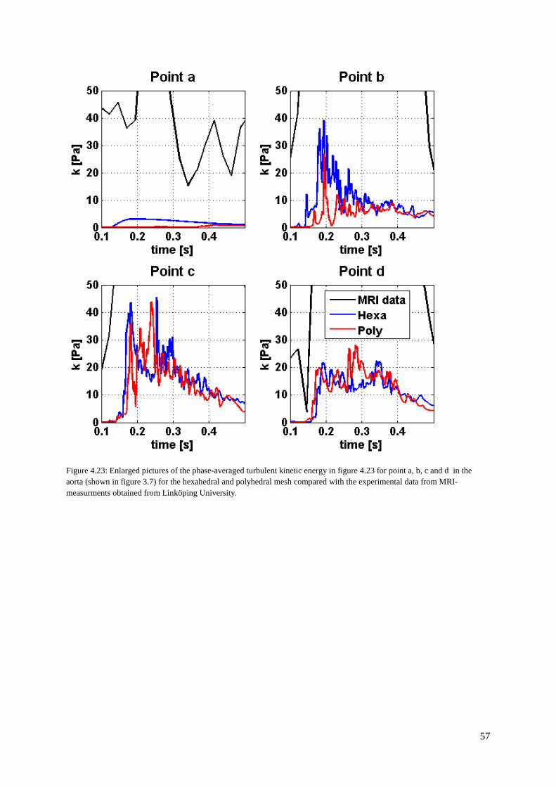
57

Figure 4.23: Enlarged pictures of the phase-averaged turbulent kinetic energy in figure 4.23 for point a, b, c and d in the aorta (shown in figure 3.7) for the hexahedral and polyhedral mesh compared with the experimental data from MRI-measurments obtained from Linköping University.

58

Figure 4.24: The phase-average of the �-velocity for a cardiac cycle for point c in the aorta (shown in figure 3.7) for the hexahedral and polyhedral mesh compared with the experimental data from MRI measurments obtained from Linköping University. Further displayed is the time-average of the results over the whole phased-averaged pulse, 0 to 1 s, and a time-average from 0.1s to 0.5s.

Table 4.2: The time-averaged results for the intervals 0 to1 s and 0.1 to 0.5 s and the difference between the MRI and the two meshes simulated at point b (shown in figure 3.7) for all three velocity components. The difference between the MRI value and the simulated results are showing the magnitude of the difference. Negative values represent a under prediction of the result and a positive value represent a over prediction of the result. The MRI results were measured at Linköping Uviversity Hospital and provided by Linköping University.

Point b �

[m/s] � diff [m/s]

� [m/s]

� diff [m/s]

� [m/s]

� diff [m/s]

� [m/s]

� diff [m/s]

0 - 1 s MRI -0.017 - 0.070 - 0.016 - 79.582 -

Hexa 0.014 0.032 0.134 0.064 -0.128 0.144 4.220 75.362

Poly 0.012 0.029 0.150 0.080 -0.123 0.139 2.417 77.165

0.1 - 0.5 s MRI 0.121 - 0.195 - -0.115 - 146.918 -

Hexa 0.062 0.058 0.328 0.134 0.328 0.443 9.109 137.809

Poly 0.056 0.065 0.372 0.177 -0.231 0.116 5.024 141.894

59

Table 4.3: The time-averaged results for the intervals 0 to1 s and 0.1 to 0.5 s and the difference between the MRI and the two meshes simulated at point c (shown in figure 3.7) for all three velocity components. The difference between the MRI value and the simulated results are showing the magnitude of the difference. Negative values represent a under prediction of the result and a positive value represent a over prediction of the result. The MRI results were measured at Linköping Uviversity Hospital and provided by Linköping University.

Point c �


� [m/s]

� diff [m/s]

� [m/s]

� diff [m/s]

� [m/s]

� diff [m/s]

0 - 1 s MRI 0.042 - -0.017 - 0.120 - 73.447 -

Hexa 0.038 0.004 -0.001 0.016 -0.110 0.230 6.476 66.971

Poly 0.028 0.014 -0.013 0.004 -0.083 0.204 5.611 67.836

0.1 - 0.5 s MRI 0.140 - -0.003 - 0.116 - 129.982 -

Hexa 0.148 0.008 -0.015 0.012 -0.015 0.131 14.421 115.561

Poly 0.121 0.018 -0.013 0.010 -0.157 0.273 12.825 117.158 Table 4.4 The time-averaged results for the intervals 0 to1 s and 0.1 to 0.5 s and the difference between the MRI and the two meshes simulated at point d (shown in figure 3.7) for all three velocity components. The difference between the MRI value and the simulated results are showing the magnitude of the difference. Negative values represent a under prediction of the result and a positive value represent a over prediction of the result. The MRI results were measured at Linköping Uviversity Hospital and provided by Linköping University.

Point d �


� [m/s]

� diff [m/s]

� [m/s]

� diff [m/s]

� [m/s]

� diff [m/s]

0 - 1 s MRI 0.009 - -0.022 - 0.088 - 63.386 -

Hexa 0.006 0.003 -0.015 0.007 -0.080 0.168 4.970 58.416

Poly 0.013 0.004 -0.011 0.011 -0.059 0.147 5.224 58.161

0.1 - 0.5 s MRI 0.090 - 0.004 - 0.105 - 117.258 -

Hexa 0.077 0.013 -0.056 0.060 -0.056 0.162 10.663 106.595

Poly 0.093 0.003 -0.037 0.041 -0.128 0.233 11.706 105.552

60

5. Discussion

5.1 Test case 1 – cylinder

5.1.1 Stagnation point and top vortex For the stagnation point, there seem to be a general pattern of how the simulated results group, at least in the z-direction with some small exceptions (figure 4.5). Generally speaking, the RANS solutions are located at the highest locations seen in the z-direction of the simulated results. The SAS model gives results that are located closer to the experimental value than for RANS, but the LES results are located on an even better z-location. One exception for this reasoning is the location of MS3 RANS, which gives the best agreement of the z-coordinate with a difference of 0.7 percent. However, this tendency does not hold when looking at the results in the x-direction, since there is no general detectable pattern at all. The best agreement in the x-direction is for MS2 LES with a difference of 0.2 percent. The best agreement when looking on the absolute value of the distance to the experimental value is for MS1 LES ��<1, with a deviation of 13 percent. There is a tendency that the results for the finer meshes are closer to the experimental result than the coarsest meshes for all simulation methods. One exception is for MS1 SAS, which lies in the neighbourhood of the results of the finer meshes.

The agreement with the experimental result of the stagnation point is not that good for any of the simulated cases. The expectation of changing the inlet turbulence intensities and running a mesh with lower �� was to see if the results could become better, but no large improvements were obtained of the stagnation point prediction. None of the obtained results over-predict the x-value of the stagnation point and all of them are under-predicting the measured location. Despite our efforts to make the result to better agree with the experimental value was this not achieved, at least from the stagnation point of view.

With some small exceptions, the top vortices lie, more or less, on the same height (z-direction) (figure 4.6) in line with the experimental result. The RANS results are close to each other and are fairly close to the experimental location of the vortex centre. All SAS results, except MS1 ��<1, are grouped at two locations; one just a short distance to the left of the experimental value and one further away to the left of the experimental result close to the cylinder surface. The LES results are spread out over the cylinder top. The overall best agreement the MS1 ��<1 RANS has, with the absolute difference of 10 percent. It has a very good agreement in the z-direction with a difference of only 0.01 percent.

Another interesting thing to notice for the lower�� cases for SAS and LES is that two vortices on the top of the cylinder are formed, instead of only one as for the other simulated cases and the experimental result. One possible explanation for this could be the fact that the front vortex is located closer to the front edge, leaving much space behind itself, which in turn leads to the generation of a second vortex.

There do not seem to be any correlation between the results for the stagnation point and the top vortices. In addition, no connection was found between the stagnation point or the top vortices with the other of the variables that have been studied like �� or Strouhal number for example. The stagnation point and the top vortices affect the flow, but they do not seem to be the most important factors for the overall predictions of the flow properties.

61

5.1.2 Q-criterion and eddy viscosity The figures of the Q-criterion (figure 4.7, 4.8 and 4.9) show clearly how well the different simulation methods resolve the turbulent eddies in the flow. The RANS solutions are very rough with large structures, which occur due to the time-averaging procedure that is introduced by the Reynolds decomposition in the flow equations. For SAS, the structures are finer than for RANS which indicates that the SAS model computes the turbulence in the flow better. The LES results have even smaller structures of the Q-criterion, which is because it resolves the large structures directly without any time-averaging assumption as in RANS. How small these large structures will be in the LES computations is limited by the grid size, which is very apparent when comparing MS1 LES with MS2 LES where the element size is halved.

As mentioned in section 2.5.1, the SAS model can have problems to switch to LES-mode when the turbulence in the flow is low. The results for the Q-criterion, eddy viscosity and the time statistics support that the SAS model has switched from RANS to a LES-like behaviour, since these figures for SAS are more LES-like, rather than RANS-like. From the Q-criterion it is seen that the size and intensity of the structures become more similar to those structures that are seen in the LES results. This is also supported by the eddy viscosity (figure 4.10) where the viscosity is decreased for SAS compared to the RANS model, but not as low as for LES, and by the flow field (figure 4.11) where the SAS model looks more like LES rather than RANS. Even though SAS appears to calculate more like LES rather than RANS, the solution is not equivalent to a LES solution. In figure 4.10 it is seen that as the cell size decreases, the eddy viscosity also decreases, which is an indication that the solution for MS2 and MS3 should be even more LES-like than for MS1 SAS.

An explanation for why the SAS model does not generate as good results as for the LES model could be found in the difference in their flow equations. In LES �� in the free stream depends on the cell size (equation 2.62-63), whilst in the SAS model it depends on the ratio between � and ��,� (equation 2.69-71), which makes the SAS model including more approximations than the LES model which in the end lead to worse predictions of the flow. The SAS model is still a RANS solver with some improvements that give better flow predictions than a regular RANS solver. It still only models the turbulence in the flow, it never resolves the turbulent eddies as the LES does, which still seems to be the best method for getting results with good precision.

5.1.3 Lowering of �� The RANS method shows a significant �� dependency (average ��

= 0.19) with a drastically improved drag coefficient, Strouhal number and top vortex position compared to the original MS1 (average ��

= 24). The lowering of �� also leads to a changed view of the Q-criterion and the eddy viscosity. For the Q-criterion, smaller structures are seen close to the cylinder wall and the rotating structures in the free stream flow become larger and more widely spread. Furthermore, an interesting thing is that the eddy viscosity is much higher for the case with low �� on RANS, than for the other RANS simulations (figure A.1 in appendix A8). For the other two models, SAS and LES, the lowered �� gives the same decrease in the separation angle and Strouhal number, as for RANS (figure 4.3 and 4.12), but a decrease in the drag coefficient (figure 4.1) which was instead increased for RANS. It is obvious that the wall functions, used in the RANS case, do not give good results. For this flow situation it would have been better to have used meshes with �� less than one for all the RANS simulations for getting better results. However, as mentioned earlier, the same improvement of the results were not obtained for the SAS and LES models. The SAS model seems to not be that dependent on the use of wall functions as the RANS model. The main focus of this study was on the SAS model why any further investigations, with �� less than one, were performed. The aim was to

62

perform simulations from an engineering perspective which means that meshes with well resolved boundary layers are often difficult to do.

A possible explanation for the lowered �� effect for the LES model is that LES is better at handling large eddies (structures). By introducing smaller elements, the size of the resolved structures becomes smaller close to the cylinder. By not refining the rest of the mesh the new gained information could get lost when it reaches the larger elements if the structures are smaller than the cells, which leads to no large improvement of the results. Keep in mind that the lower �� is not obtained on the cost of the rest of the mesh, the extra cells that arise due to the refinement close to the cylinder are added to the total number of cells in the mesh. In this case, the only structures that will get lost are the structures that are growing slower than the growth rate of the cells. Parts of the argument for LES can be used for the SAS case, by using smaller elements the SAS model could be forced to use the LES mode. The length scale that it uses for determining the switch between RANS and LES mode (equation 2.68) depends both on the turbulence in the flow and the grid size. The smaller elements on the cylinder surface could have trigged SAS to compute the flow in these regions with LES qualities which may not be favourable in this case since RANS is better at predicting the boundary layer when the wall functions are excluded. To avoid this loss of information in the results, we should have done a better mesh by instead using a smaller growth rate between these two mesh regions or refined the rest of the mesh too to ensure that all of the gained turbulent eddies were included further downstream.

5.1.4 Drag coefficient The best prediction of �� is for MP1 LES as seen in figure 4.1, with the percentage difference of 0.4, which is the only result that is over-predicting the experimental result. The RANS solution with ��<1 gives a large improvement of 64 percent compared to the MS1 case which has an average of��

= 24. The best �� for SAS is for the cases with increased turbulence intensity at the inlet, which differs with 9 percent compared to the experimental value.

The overall tendency, as seen in figure 4.2, is that �� is improved when changing from RANS to SAS, and further improved when changing to LES. Furthermore, the results become worse when the size of the elements in the wake is reduced for all the different mesh types and simulation methods (figure 4.2). The polyhedral elements give better results than the tetrahedral and hexahedral, where the tetrahedrals are the worst. It is not that surprising that the polyhedral meshes perform better results than the other two cell types, since the Fluent solver interpolates the value of the cell from the cell faces. The polyhedral elements are performing calculations on two more cell faces compared to a hexahedral and four compared to a tetrahedral element. By comparing the wake width (figure 4.13, 4.14, 4.15 and 4.16) and �� (figure 4.1) for each turbulence model, there seems to be a strong connection between these two parameters. The wider the wake the better prediction of ��. Some exceptions are present as for MO2 RANS that has one of the worst �� predictions, but the wake width prediction is in the middle of the other results. However, there is another difference in MO2, it over-predicts the length of the wake at X/D=6. The form of the MO2 wake profile is different than the others since it is narrow and long, whilst most of the other wakes have the same form as the experimental wake but narrower and shorter. The theory about the importance of the width of the wake that was discussed earlier is also supported by the fact that the wake becomes wider when changing simulation model to SAS and LES (figure 4.17). For the velocity profiles it is seen that at the location further away from the cylinder, the better the predictions becomes.

As mentioned earlier, the fact that there do not seem to be a coupling between the stagnation point and �� suggests that this is not the most important variable for predicting the drag coefficient. On the other hand, the width of the wake shows a stronger coupling with the drag, which leads to a conclusion that

63

the width of the wake is more important than the length of the wake for predicting ��. This idea is also supported by the results for the RANS case with low�� where the stagnation point lies in the middle of the other results, but the wake width is considerably wider than the other profiles at X=6D and X=10D and gives a good prediction of the drag coefficient.

The separation angle is a factor that in theory should contribute to the width of the wake and thereby the drag coefficient. In figure 4.12, which shows the separation angle, the trend is that the angle decreases when the simulation model is changed from RANS to SAS and further to LES. However, when �� is lowered, the separation angle decreases for all simulation models but the drag coefficient is only increased for the RANS case, which leads to the suggestion that an earlier separation from the cylinder surface does not affect �� in a large extent in this case.

5.1.5 Strouhal number The best agreement with the experimental Strouhal number the MS1with �� <1 for RANS and SAS has, with the percentage difference of 3 and 5 percent, respectively. The second best agreement has MP1 RANS with the difference of 11 percent.

When comparing the drag coefficient results (figure 4.1) with the Strouhal number results (figure 4.3), not exactly the same pattern is visible. For example, MS1 SAS gives better drag coefficient than MS1 SAS with low��, but the opposite is seen for the Strouhal number. The same thing is seen for MS1 with increased turbulence intensity compared with MS1, and MS3 RANS compared with MS2 RANS. By looking at the averaged results in figure 4.4 it is also seen, as for the drag coefficient in figure 4.2, that the polyhedral meshes give better results than the tetrahedral and hexahedral meshes that have almost the same agreement for both the drag coefficient and Strouhal number. For the Strouhal number MO1 and MO2 has the same agreement, but for the drag coefficient there is a remarkable difference.

By looking at the time statistics of �� in figure 4.18 one sees that there is a large difference between RANS and the SAS and LES statistics. RANS has not that large amplitude as SAS and LES and it also has a higher frequency, which is also seen in figure 4.3 with the Strouhal number, which is uniform over time. By instead comparing SAS and LES one sees that they have a similar behaviour and have almost the same frequency, which was also seen in figure 4.3 with the Strouhal numbers. The frequency of LES is more dominating since it has higher amplitude, which was also seen in figure 4.11. Another interesting thing to notice in this figure that has been mentioned before is that SAS has definitely switched into LES mode, since their statistics are more similar than for RANS, but they are not exactly the same. For the SAS solution, it looks like the dominating shedding frequency is dampened with increasing simulation time and becomes more like a RANS solution with a more uniform frequency and lower amplitude. A farfetched idea is that the turbulence is constantly dampened so that the turbulence in the flow becomes destroyed and thereby successively leads to a switch into RANS mode. It would have been interesting to run the simulations a longer time to see how the time statistics and overall results would have looked like after a longer simulation time. Would the SAS solution become a RANS solution after a while? In the reasoning of the switch into LES mode and that the solutions looks almost like LES, the results of the flow parameters are not that LES-like. This could be explained by the flow not being turbulent enough for getting so good results that could be possible with the SAS model. As mentioned before, if the flow is not turbulent enough it has problems with switching into LES mode. If the unsteadiness in the flow is not turbulent enough the switch is delayed because it takes a while before the SAS model gets trigged and turns into LES mode which affects the results negatively. It is mainly seen in the time-averaged results as the drag coefficient, Strouhal number, separation angle, velocity profile, top vortex and stagnation point, but

64

the Q-criterion, eddy viscosity and the velocity field are instantaneous pictures for the latest time steps in the solution where the SAS model have switched into the LES mode.

5.1.6 Cell refinement It has been discussed earlier that the results get worse with a finer mesh for almost all simulated cases. The meshes that satisfy the requirements that ANSYS postulates, which is a cell size of at least D/20 and 10-15 prismatic layers covering the boundary layer, are only the MS2 and MS3 meshes and are those that theoretically should give the best results. It is strange that the agreement with the experimental results became worse for those meshes compared to the coarser mesh MS1. It has been noticed that for the Strouhal number and the wake profiles, there is a smaller percentage difference between MS3 and MS2 than between MS1 and MS2. A possible explanation for this could be that the results are becoming less mesh dependent and are converging to the results that the simulation methods deem to be correct. If it is so, then it raises the question if it is the measurements or the simulation methods that are giving the incorrect results? Since the measurements not have been performed by ourselves and are not further described in the papers that we have taken the data from, we could not answer the question of how accurate the experimental results are. It is mentioned in the papers [7] that the approximated uncertainty of the mean velocity measurements was two percent, so the experimental results should not be that wrong. The viscosity and density used in the experiments were not stated in the articles, but they could be calculated from the Reynolds number that was stated in the articles. However the density and viscosity that were used was based on air for 1 atm, but the pressure where the measurements were performed was unknown. This should have had a very small affect on the results since the Reynolds number was the same as for the measurements. Wall roughness for the cylinder and the floor affects the boundary layer, which were also unknown and highly affects the results. Furthermore, as mentioned in the method section, no true mesh independency study was done for neither of the test cases, so the results might still be mesh dependent. This is indicated by the results of the meshes with different element sizes that differ from each other.

5.1.7 Change of turbulence intensity Two simulations were run with different turbulence intensities compared to the original turbulence intensity, which was made to see how dependent the SAS model is on the inlet turbulence intensity. To induce this, both the turbulence intensity and the viscosity ratio were changed to make two worst case scenarios. The result of that was that the drag coefficient and the wake profile predictions became better than for the original case, but the Strouhal number became worse for both cases. The case with lowered turbulence intensity follows the theory that the flow separates earlier when the turbulence is low and thereby increases the drag coefficient. On the other hand, the results for the increased turbulence intensity do not confirm the theory that the drag should decrease when the turbulence is increased. A possible explanation for this lies in the formulation of the SAS model which says that if the flow becomes turbulent, the SAS model should switch from RANS to LES mode. If so, a larger part of the flow field is computed with the LES mode than for the base case MS1, making the overall solution look more like the LES solution and therefore gives a better prediction of the drag coefficient.

5.1.8 Time requirements The simulations for MP1 and MS1 ��<1 have been run on the same cluster, number of cores, RAM-memory and time step, respectively. The comparison in table 4.1 shows unexpected results of the difference in computational time for the different simulation methods. It was expected that RANS would have the shortest time requirement and LES the longest, not the opposite. A theory for why the RANS computations were that slow could be that this simulation was complicated to compute by RANS. It have been noticed that the LES simulations needed less subiterations than RANS, which is probably the reason for the longer simulation times for RANS. This is just a speculation, since this

65

was only noticed and not monitored, no definite explanation can be said from that information. Another idea is the fact that RANS needs to compute two extra differential equations, the transport equations, which are not included in the LES computations and therefore is taking longer to compute the result than the LES model. In addition to this, the SAS model needs to compute the extra variable �� (equation 2.69), which could be the explanation for why the SAS model is even slower than the RANS model.

As seen from the time statistics in figure 4.18, the RANS solution becomes stable much faster than the SAS and LES solutions. The RANS solution could be said to be stabilized after 0.04 s whilst for SAS and LES the solution never reaches the same stable behaviour and was needed to be run for at least 0.5 s and maybe longer. So, in the long run, the RANS model is the simulation model that will lead to the shortest computational time to get good statistics.

5.1.9 Method The RANS-SST model was chosen for the reason that the only SAS model available in Fluent is the SAS-SST model. Other turbulence models than the SST model for RANS could have been analyzed to see if other models are better for this specific flow case, but since the main objective of this thesis was to evaluate the SAS model was this investigation excluded.

The determination of the time requirements for the different simulated cases could have been done in another way to get more appropriate comparisons of all simulated cases. First of all, the simulations would have been run on the same cluster and same number of CPU’s. On the other hand, if we would have done that we would not have run that many simulation cases within the time that was purposed for this thesis and the investigation would not have been that thorough. The second thing that could have been made different to get a better comparison of the time requirements would have been to monitor the required number of subiterations it took for each time step to converge. It would have been useful to get some statistics of that for getting a better understanding of the computations for each model and element type.

If the goal was to get as good agreement as possible with the experimental results all meshes would have been done with �� less than one, be mesh independent and satisfy ANSYS recommendations. The aim of this thesis was to perform simulations from an engineering perspective, why the meshes were made fairly coarse and no mesh independency study was done, so the three simulation methods were evaluated from that standpoint. With this in mind, it could be concluded that the SAS and LES results gives satisfactory results even with a coarse mesh. From our results, it could even be concluded that the results become better with a coarser mesh for all simulation methods. This conclusion is not correct from a theoretical point of view, but it is what our results are showing.

5.2 Test case 2 – Aorta

5.2.1 Results None of the phase-averaged results are that smooth as the MRI result (figure 4.19, 4.20, 4.21 and 4.22), but follows the characteristic of the pulse, especially the �- and -velocity. The reason for why the phase-averaged curves are not that smooth is probably because the simulations would have needed to be run for more cycles, than the eight cycles that were simulated. Due to the short amount of time left to deadline, when the simulations of the aorta began and the large time requirements for the simulations, it was not feasible to simulate additional pulses.

The results of the velocity components agree fairly well with the MRI-measurements as seen in figure 4.19, 4.20 and 4.21 and in table 4.2, 4.3 and 4.4 for each of the points in the aorta. They follow the

66

behaviour of the experimental results well and the magnitude is acceptably good with some small exceptions. When looking at the turbulent kinetic energy in figure 4.22 and 4.23 the results are very poor. The behaviour during the pulse is caught, but the magnitude is totally wrong and it under-predicts at all points. At point a, which is close to the main inlet, is close to zero for SAS, but the time-average of the MRI-result it is 33 Pa. This could be an indication of that the turbulence intensity set at the inlet was probably too low compared to the experiments. At the other points b, c and d, is also under-predicted, however at these points the flow has passed through an almost 90 degree bend, two branching vessels and the coarcatation, so the flow is very likely turbulent at these points which should have trigged the SAS model to switch into LES mode. Probably the flow is not unsteady enough for getting a fast switch into the LES mode for getting good results as explained before for the cylinder case.

If the inlet flow is time dependent, as in this case, the mean values (for example �, � and ) can be seen as the phase-average variables. In the aorta case that would mean that the phase-averaged velocities in figure 4.19, 4.20 and 4.21 are the time-averaged velocity components in the Reynolds decomposition (equation 2.10). Even if the fluctuations in the flow are miscalculated, the mean flow components could still be accurate if the magnitude of the fluctuations were wrong. This could be used for explaining, based on our results, why the velocities have a better agreement with the MRI-results than the turbulent kinetic energy, , which is based on the velocity fluctuations in the flow. The simulation model produces acceptable time-averaged results, but is weak at predicting the unsteadiness in the flow, which leads to the under-prediction of .

There is a question if the SAS model is performing the calculation in RANS or LES mode. As mentioned before, the flow after the coarcatation is turbulent and should be sufficiently turbulent for making the SAS model to switch to LES mode. The disadvantage with the SAS model is that it may not switch into LES mode at all or delays the switch, which was mentioned before, if the flow is not turbulent enough. The under-predicted could be an indication of that the SAS model have not turned into LES mode, where the fluctuations are allowed to become larger due to the fact that the eddy viscosity is lowered.

The flow is probably not turbulent enough to get good results with the SAS model due to the reasoning that it does not switch into LES mode that was discussed above. The same poor results have been obtained in other studies performed on the same aorta by Lantz et al. [20]. In their study, the SAS-SST model performed even worse prediction of than the RANS-SST model, which is very strange. If the SAS model does not switch into LES the results should be computed with RANS-SST and should give the same results as the standard RANS-SST model.

In the cylinder case, one of the conclusions was that the polyhedral mesh performed better results than the hexahedral mesh and that the results, with some exceptions, under-predicted the results. In the aorta case, by looking in table 4.2, 4.3 and 4.4, the number of cases the hexahedral respectively the polyhedral mesh performed better results are almost the same. The hexahedral mesh predicts the flow better than the polyhedral only once in total and the majority of the results are under-predicting the experimental result just as in the cylinder case.

5.2.2 Method The used turbulence intensity at the inlet was an approximated value. It would have been better to have used the turbulence intensity from the MRI-measurements at the inlet to make the simulations as correct as possible. This idea came up when the simulations were already running and there was not enough time left of this thesis for running new simulations. Either way, the SAS results would

67

probably have been unsatisfactory anyway which could be strengthened with the study performed by Lantz et al. [20] that was mentioned before. No mesh independency study was performed for this test case either, but a low �� and CFL number should have captured the dynamics of the flow well and should have given reasonably correct results.

It would have been interesting to investigate the aorta case more thoroughly than it has been done in this thesis. The expected time requirement for this test case was too short, since unexpected problems occurred when setting up the problem. To make the comparison of the results easier and better, the mesh was transformed into the same coordinate system as for the MRI-measurements, which was not that easy because they were totally different and therefore it took long time to make them correlated. Furthermore, the complex geometry of the aorta gave problems with the meshing, especially for the polyhedral mesh, since the block structure for the hexahedral mesh was already done when we got it from the university.

The mentioned transformation of the coordinate system was made in ANSA where the modelled aorta was translated and rotated so it visibly correlated with the original MRI-aorta scans. Since this was done manually there is a possibility that there are some deviations between the coordinate systems that can lead to a disagreement between the simulated results and the MRI results. Furthermore, the walls of the aorta were smoothed to make it possible to perform a mesh on which computations could be made. Additionally, some arteries that were present in the original geometry were removed from the simulation model for simplifying the calculations. Both actions affect the results, but should have not affected the results in a large extent. Another simplification that was made was the fact that the wall of the aorta was assumed to be rigid and that the flow was incompressible, which is not the case in a real aorta and could have an impact on the velocity and pressure calculations. The MRI-measurements have not that good resolution as mentioned in section 3.2. The diameter is covered with only 24 measurement points which could have an effect on the results for the turbulent kinetic energy since the fluctuations, the small eddies, maybe are not captured with a so coarse grid.

68

6. Conclusions From our results it could be concluded that the LES model, in many of our test cases, was the fastest model for computing the simulations and the SAS model was the slowest. The time it took for the time-statistics to reach a stable solution was approximately the same for these two models. The computations performed by the LES model gave the best overall results with a good agreement with experimental data. The second best agreement had the SAS results. So from the first test case it could be concluded that there do not seem to be any advantage of running the simulations with the SAS model compared to LES since it performs worse results and is more time consuming than both LES and RANS.

As discussed before, particularly in section 5.1.1, there were difficulties of discerning the connections between the top vortex and the wake behind the cylinder with the drag coefficient and Strouhal number, which was expected from the flow situation as described in the introduction. From our results it could be concluded that this flow situation has been more difficult to compute for all simulation methods since the overall obtained results are not as good as one would have expected for both RANS and LES.

As concluded in the discussion, the mesh type in the first test case that gave the best results was the polyhedral mesh. No conclusion of which element size is preferable for each simulation model is drawn, since the reason for why the results became worse with finer mesh is unknown.

From the results obtained for both the cylinder and aorta test case, it could be concluded that the SAS model is not suitable for flows with moderate Reynolds numbers since the switch to LES mode becomes delayed or does not switch at all which affect the results negatively.

69

7. Further work Since our study only contained two test cases, only one of them were deeply investigated, it would be appropriate to evaluate some other applications before any absolute decisions when the SAS model is applicable and when it is not, is made. The developer of the SAS model presents results [5] by SAS which have very good agreement with measurements and are comparable with LES results. Probably there are other flow cases for which the SAS model is suitable and performs good results and maybe is not that time consuming as for our test cases. These applications are needed to be found and documented since we have seen from our results that the precision can vary very much depending on flow situation and flow parameters. From FS Dynamics’s point of view, it would be interesting to see if it would be possible to run SAS simulations on coarser meshes and larger time steps, compared with what is necessary to use in LES computations with the hope of finding that the SAS model could be used on coarser meshes and larger time steps and thereby shorten the simulation time but still get better results than for RANS. Since the concept of hybrid models still is interesting for them, it would be interesting to evaluate other hybrid models on the same test cases to see how well they perform the same flow situation. Another suggestion of further work is to run simulations of the cylinder case with a higher Reynolds number and thereby see if the results would have been improved when the flow is more turbulent. Additionally, as suggested in the discussion, it would be interesting to run the MS1 SAS simulation a longer time to see if the computations transforms into RANS.

For the second test it would be interesting to simulate cases with RANS and LES and compare them with our SAS simulations, since LES results performed by Lantz et al. [15, 20] gave good agreement with the MRI-measurements. This could confirm whether the SAS model have switched from RANS to LES mode or not. Based on the suggestion of evaluation the SAS model on other flow simulations the aorta could be divided into two flow situations; a basic pipe flow and a jet flow, to lower the complexity. These two suggested test cases would be interesting to simulate and maybe find a better explanation for why the SAS model has difficulties with the flow in the aorta.

70

8. References [1] H. K. Versteeg, W. Malalasekera, An introduction to computational fluid dynamics the

finite volume method, second edition 2007, Ashford Colours Press Gosport Hants. [2] L. Davidson, Fluid mechanics, turbulent flow and turbulence modeling, Division of

fluid dynamics Chalmers University of Technology, 2012 [3] D. C. Wilcox, Turbulence modeling for CFD, second edition, California 1998 [4] F. R Menter, Best Practice: Scale- Resolving Simulations in ANSYS CFD, version 1.0,

2012, ANSYS Germany [5] F. Menter, Y. Egorov, The Scale- Adaptive Simulation Method for Unsteady Turbulent

Flow Predictions. Part 1: Theory and Model Description, Springer, Ansys Germany, 2009

[6] Scale-Adaptive Simulation Theory, Theory guide ANSYS CFX/ Fluent [7] N. Rostamy, D. Sumner, D. J. Bergstrom, J. D. Bugg, Local flow field of a surface-

mounted finite cylinder, Department of Mechanical Engineering, University of Saskatchewan, Elsevier Ltd., 2012

[8] M. S. Adaramola, O. G. Akinlade, D. Sumner, D. J. Bergstrom, A. J. Schenstead, Turbulent wake of a finite circular cylinder of small aspect ratio, Division of Environmental Engineering and Department of Mechanical Engineering, University of Saskatchewan, Elsevier Ltd., 2006

[9] D. Sumner, O. J. P. Dansereau, J. L Heseltine, Vortex shedding from a finite circular cylinder of small aspect ratio, Department of Mechanical Engineering, University of Saskatchewan, 2004

[10] D. Sumner, J. L. Heseltine, O. J. P. Dansereau, Wake structure of a finite circular

cylinder of small aspect ratio, Springer-Verlag, 2004 [11] T. Kawamura, M. Hiwada, T. Hibino, I. Mabuchi, M. Kumada, Flow around a Finite

Circular Cylinder on a Flat Plate, Bulletin of JSME, Vol. 27, No. 232, 1984 [12] H. F. Wang, Y. Zhou, J. Mi, Effects of aspect ratio on the drag of a wall-mounted

finite-length cylinder in subcritical and critical regimes, Springer-Verlag, 2012 [13] ANSYS FLUENT Theory Guide, ANSYS, Inc., Release 14.0, 2011

[14] ANSYS FLUENT User’s Guide, ANSYS, Inc., Release 14.0, 2011

[15] J. Lantz, On Aortic Blood Flow Simulations – Scale-Resolved Image Based CFD, Linköping University, 2013

71

[16] E. Bruckheimer, CA Cardoso Pedra, Stenting Optionsfor coarctation of the aorta, Schneider Children’s Medical center Israel, Instituto Dante Pazzanese de Cardiologia

[17] http://www.seattlechildrens.org/medical-conditions/heart-blood-conditions/coarctation-of-the-aorta/, 2013-04-04

[18] J. Bogaert, Clinical cardiac MRI, Springer 2012, New York

[19] F. Nicoud, F. Ducros, Subgrid-scale stress modelling based on the square of the velocity gradient tensor, CERFACS- Centre Européen de Recherche et de Formation Avancée en Calcul Scientifique, 1999

[20] J. Lantz, Tino Ebbers, Jan Engvall, Matts Karlsson, Numerical and Experimental Assessment of Turbulent Kinetic Energy in an Aortic Coarctation, Department of Management and Engineering, Department of Science and Technology, Department of Medical and Health Sciences, Linköping University, 2013

[21] F. Menter, Y. Egorov, R. Lechner, D. Cokljat, The Scale- Adaptive Simulation Method for Unsteady Turbulent Flow Predictions. Part 2: Application to Complex Flows, Ansys Germany and Ansys United Kingdom

72

Appendix A

A1. Numerical setup test case 1 Since it was the continuity equation that was the slowest equation to converge was the under-relaxation factor varied for the different simulation cases trying to get faster simulations. The other variables were the same for all simulations. In table A.1 are the ranges of the used under-relaxation factors for the different grids presented for the different simulation models.

Table A.1: Used under-relaxation factors for the three different simulation models used in test case 1. For the pressure the ranges of the used under-relaxation factors for the different grids are presented.

Under Relaxation Factors – test case 1

RANS SAS LES

Pressure 0.3 -0.7 0.6-1.0 0.8

Density 1.0 1.0 1.0

Body Forces 1.0 1.0 1.0

Momentum 0.7 0.8 0.8

Turbulent Kinetic Energy

0.8 0.8 -

Specific Dissipation Rate

0.8 0.8 -

Turbulent Viscosity 1.0 1.0 -

A2. Mesh information test case 1 In table A.2 is information about the different meshes presented in terms of number of elements and average �� on the cylinder surface.

Table A.2: Number of elements and average �� on the cylinder for the different meshes and simulation cases for test case 1.

Mesh information – test case 1

Number of elements

RANS ��

SAS ��

LES ��

MS1 2 744 576 24.49 28.01 29.46

MO1 5 636 310 31.93 31.03 29.04

MP1 1 024 413 30.16 31.94 29.06

MS2 7 933 400 23.61 23.76 -

MO2 40 242 797 33.50 32.63 -

MP2 7 078 994 30.63 30.63 -

MS3 25 837 037 23.15 23.36 -

MS1 y+<1 3 012 616 0.19 0.19 0.19 MS1_lowTurbInt 2 744 576 - 30.54 - MS1_highTurbInt 2 744 576 - 30.46 -

73

A3. Numerical setup test case 2 In table A.3 the under-relaxation factors that have been used for the two aorta simulations are presented.

Table A.3: Used under-relaxation factors for the simulations in test case 2.

Under-relaxation factors - test case 2 SAS

Pressure 0.6

Density 1.0

Body Forces 1.0

Momentum 0.9

Turbulent Kinetic Energy

0.9

Specific Dissipation Rate

0.8

Turbulent Viscosity 1.0

A4. Mesh information test case 2 In table A.4 information about the meshes used in test case 2 in terms of number of elements and average �� on the arterial wall are presented.

Table A.4: Number of elements and average ��on the arterial wall for test case 2.

Mesh information – test case 2

Hexahedral Polyhedral

Number of elements 2 870 950 2 458 114

�� 0.57 0.15

A5. Stagnation point locations In table A.5 are the stagnation point coordinates presented and their percentage difference compared to experimental values.

74

Table A.5: Locations of the stagnation point corresponding to symbols in figure 4.5 and their percentage difference compared to experimental data.

Stagnation point locations RANS SAS LES

X·D diff X

[%]

Z·D diff Z

[%]

X·D diff X

[%]

Z·D diff Z

[%]

X·D diff X

[%]

Z·D diff Z

[%] MO1 1.80 40 3.60 24 1.58 47 2.75 5 1.63 46 3.25 12 MO2 2.38 21 4.33 49 2.25 25 3.75 29 - - - - MS1 1.80 40 3.60 24 2.00 33 3.33 15 1.58 47 2.50 21 MS2 1.68 44 3.23 11 1.90 37 3.75 29 2.40 0.2 2.85 33 MS3 1.75 42 2.92 0.7 1.83 39 3.75 29 - - - - MP1 1.75 42 3.90 34 1.29 57 3.25 12 1.58 47 2.33 15 MP2 - - - - 2.17 28 2.75 5 - - - - MS1 y+<1

2.04 68 3.61 24 2.60 13 3.47 20 2.46 18 2.92 35

MS1 LTI

- - - 1.72 43 3.43 18 - - - -

MS1 HTI

- - 1.46 2.93 - -

A6. Top vortex locations In table A.6 are the top vortex coordinates for the different simulated cases in test case 1 with their percentage difference compared to experimental values.

Table A.6: Locations of the top vortex corresponding to the symbols in figure 4.6.

Top vortex locations RANS SAS LES

X·D diff X

[%]

Z·D diff Z

[%]

X·D diff X

[%]

Z·D diff Z

[%]

X·D diff X

[%]

Z·D diff Z [%]

MO1 -0.013 78 9.063 0.2 -0.132 120 9.051 0.3 -0.138 130 9.057 0.3

MO2 0.016 27 9.056 0.3 -0.108 80 9.040 0.4 - - - -

MS1 -0.041 32 9.042 0.4 -0.224 273 9.000 0.9 -0.011 82 9.026 0.6

MS2 -0.048 80 9.048 0.4 -0.102 70 9.040 0.4 -0.051 15 9.043 0.4

MS3 -0.041 32 9.048 0.4 -0.092 53 9.041 0.4 - - - -

MP1 -0.099 165 9.059 0.2 -0.135 125 9.049 0.3 -0.195 225 9.045 0.4

MP2 - - - - -0.260 333 9.016 0.7 - - - -

MS1 y+<1

-0.054 10 9.081 0.01 0.087 245 9.078 0.02 0.105 75 9.071 0.1

- - - - -0.358 497 9.052 0.3 -0.344 473 9.050 0.3

MS1 LTI

- - - - -0.233 288 9.004 0.8 - - - -

MS1 HTI

- - - - -0.231 285 9.006 0.8 - - - -

75

A8. Eddy viscosity RANS In figure A.1 is the eddy viscosity visualised for the different RANS simulations.

MO1 MO2 MP1 MS1 MS2 MS3 MS1 y+<1

Figure A.1: The eddy visocity on a xy-plane located at Z/D=5 for the RANS simulation method for all mesh types and sizes including the case with ��<1.

victoria wahlbom hellström frida alenius

Documents