Part C: Beam-Columns

BeamsBasic Formulation

The Temporal SolutionThe Spatial Solution

Rayleigh-Ritz AnalysisRayleigh’s QuotientThe Role of Initial ImperfectionsAn Alternative Approach

Higher ModesRotating Beams

Self-weightA hanging beamExperiments

Thermal Loading

Beam on an Elastic Foundation

Elastically Restrained Supports

Beams with Variable Cross-section

A beam with a constant axial force

In this section we develop the governing equation of motion for a thin,elastic, prismatic beam subject to a constant axial force:

EI, mP

x

w(x)

L

P

P

M + M

M

S

S + S∆

∆

∆

∆

w w1 2

0

R(x,t) x

F(x,t) x

Q(x,t) x∆

∆

x

x/2

(a) (b)

Beam schematic including an axial load.

It has mass per unit length m, constant flexural rigidity EI , and subjectto an axial load P . The length is L, the coordinate along the beam is x ,and the lateral (transverse) deflection is w(x , t).

The governing equation is

EI∂4w

∂x4+ P

∂2w

∂x2+m

∂2w

∂t2= F (x , t). (1)

This linear partial differential equation can be solved using standardmethods.We might expect the second-order ordinary differential equation in timeto have oscillatory solutions (given positive values of flexural rigidityetc.), however, we anticipate the dependence of the form of the temporalsolution will depend on the magnitude of the axial load.

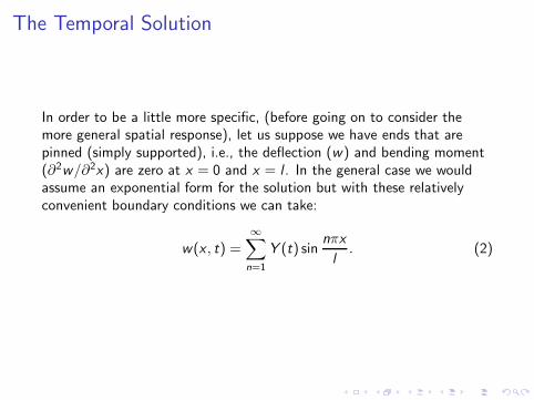
The Temporal Solution

In order to be a little more specific, (before going on to consider themore general spatial response), let us suppose we have ends that arepinned (simply supported), i.e., the deflection (w) and bending moment(∂2w/∂2x) are zero at x = 0 and x = l . In the general case we wouldassume an exponential form for the solution but with these relativelyconvenient boundary conditions we can take:

w(x , t) =∞∑

n=1

Y (t) sinnπx

l. (2)

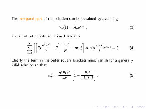
The temporal part of the solution can be obtained by assuming

Yn(t) = Aneiωnt , (3)

and substituting into equation 1 leads to

∞∑

n=1

[[

EIn2π2

l2− P

]

n2π2

l2−mω2

n

]

An sinnπx

le iωnt = 0. (4)

Clearly the term in the outer square brackets must vanish for a generallyvalid solution so that

ω2n =

n4EIπ4

ml4

[

1− Pl2

n2EIπ2

]

. (5)

If we define the following parameters:

Pcrn = n2EIπ2/l2 ω2n = n4EIπ4/ml4, (6)

equation 5 becomes

ωn = ±ωn

√

1− P/Pcrn , (7)

and we see that the nature of the solution depends crucially on thediscriminant. Making use of the Euler identities we shall consider fourrepresentative cases, where An and Bn are constants obtained from theinitial conditions.

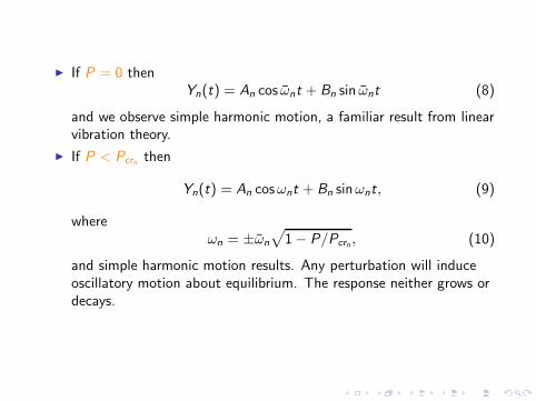
If P = 0 thenYn(t) = An cos ωnt + Bn sin ωnt (8)

and we observe simple harmonic motion, a familiar result from linearvibration theory.

If P < Pcrn then

Yn(t) = An cosωnt + Bn sinωnt, (9)

whereωn = ±ωn

√

1− P/Pcrn , (10)

and simple harmonic motion results. Any perturbation will induceoscillatory motion about equilibrium. The response neither grows ordecays.

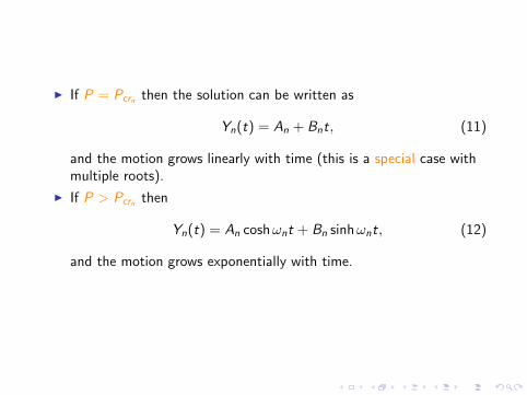
If P = Pcrn then the solution can be written as

Yn(t) = An + Bnt, (11)

and the motion grows linearly with time (this is a special case withmultiple roots).

If P > Pcrn then

Yn(t) = An coshωnt + Bn sinhωnt, (12)

and the motion grows exponentially with time.

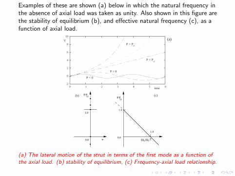
Examples of these are shown (a) below in which the natural frequency inthe absence of axial load was taken as unity. Also shown in this figure arethe stability of equilibrium (b), and effective natural frequency (c), as afunction of axial load.

-2

0

2

4

6

8

10

0 1 2 3 4 5 6

Y

time

P = 0

P < 0

P = Pcr

P > Pcr

(a)

P/P

0.0 w

1.0

0.0

1.0

P/Pcr

cr

(ω /ω )n 0

1.0

2

(b) (c)

(a) The lateral motion of the strut in terms of the first mode as a function ofthe axial load. (b) stability of equilibrium, (c) Frequency-axial load relationship.

Let’s focus attention on the lowest natural frequency and itscorresponding mode (n = 1). With no axial load (P = 0) we obtainω1 = ω1. However, as the axial load increases the natural frequencydecreases according to equation 7, i.e., we observe a linear relationshipbetween the magnitude of the axial load and the square of the naturalfrequency. Any non-zero initial conditions result in bounded motion, andwe may consider this to be a stable situation (at least in the sense ofLyapunov).

When P = Pcr1 , ω1 vanishes and the solution becomes real (the linearlyincreasing (constant velocity) solution, and any inevitable perturbationwill cause the system to become unstable. This type of instability is notoscillatory but rather monotonic since, locally, the deflections grow in onedirection (determined by the initial conditions). This type of behavior issometimes referred to as divergence. The higher modes (n > 1) willexhibit oscillations but the important practical information has beengained.

The Spatial Solution

For tensile axial loads the system does not suffer instability, and we shallsee that the lowest natural frequency increases with tensile force (insimilarity to the string).Returning to equation 1 and focusing on the free vibration problem withan external but constant axial load (F (x , t) = 0)) we can write a generalsolution to the spatial part of the solution by assumingw(x , t) = W (x) cosωt and we then have

EId4W (x)

dx4− P

d2W (x)

dx2−mω2W (x) = 0. (13)

Introducing the non-dimensional beam coordinate ζ = x/l then we canwrite a general solution to the above equation in the form

W (ζl) = c1 sinhMζ + c2 coshMζ + c3 sinNζ + c4 cosNζ, (14)

in which M and N are give by

M =√

Λ +√Λ2 +Ω2

N =√

−Λ +√Λ2 +Ω2

(15)

and using non-dimensionalized axial load and frequency:

Λ = Pl2/(2EI ) Ω2 = mω2l4/(EI ). (16)

We now apply the boundary conditions. We shall use clamped-pinned tomake things a little more interesting. At the left hand end we have thefully clamped conditions

W (0) = 0 dW (0)dx

= 0, (17)

and pinned, or simply supported, at the right hand end:

W (l) = 0 d2W (l)dx2

= 0. (18)

In fact, we assume that this support is a roller, i.e., it does not allowvertical displacement or resistance to bending moments. If the horizontaldisplacement is suppressed then membrane effects may induce additionalaxial loading - a feature to be explored in more detail later, and will proveto be an important consideration in the dynamic response ofaxially-loaded plates as well.

Plugging these boundary conditions into the general solution (equation14) and applying the condition for non-trivial solutions (i.e., setting thedeterminant equal to zero) leads to the characteristic equation

M coshM sinN − N sinhM cosN = 0. (19)

This equation can be solved numerically by assuming Λ and solving for Ωor vice versa.

The figure below shows the lowest root of this equation as the solid line(normalized with respect to the natural frequency in the absence of axialload, i.e., Λ = Λ/π2). Plotting the square of the natural frequency (partb) gives almost, but not quite, a straight line. Only tensile loads(normalized by the Euler load) are plotted in this figure.

0

5

1 0

1 5

1

Λ

Ω

(a)

2 3 4_

_

0

5

1 0

1 5

16

Λ

Ω2

(b)

12840

_

_

The relation between axial load and (a) frequency, (b) frequency squared for aclamped-pinned beam.

Also plotted in these figures (as a dashed line) is an upper bound basedon the expression

Ω =√

1 + γΛ, (20)

where γ = 0.978 for the clamped-pinned boundary conditions.

The corresponding mode shape comes from the smallest root of thecharacteristic equation given by equation 14 with the coefficients

c1 = 1, c2 = − tanhM , c3 = −M/N , c4 = (M/N) tanN , (21)

and is plotted in figure below with the modeshape normalized such thatits maximum amplitude is unity.

0 0 .2 0 .4 0 .6 0 .8 1x/L

( a ) (b )Lowest vibration mode Elastic buckling mode

0 0 .2 0 .4 0 .6 0 .8 1x/L

The mode shapes correponding to (a) the lowest natural frequency, and (b) theelastic critical load, for a clamped-pinned axially-loaded beam.

Although not apparent in the figure there are actually three curvesplotted. Superimposed on the zero-load case (a continuous curve) is themode shape when the beam is subject to a compressive load of one halfthe elastic critical load, which corresponds to U = −5.55 in the unitsused. Note that this has an almost negligible effect on the mode shapedespite the frequency dropping from Ω0 = 15.42 for the unloaded case toΩ = 10.42 (and indicated by a dotted line). Similarly a tensile force ofthis same magnitude causes the lowest natural frequency to increase toΩ = 19.09 but has only a minor influence on the mode shape (dashedline). In general, despite the relatively strong effect of an axial load onthe natural frequencies of thin beams (and strings), the effect on modeshapes is relatively minor. We shall see later that this is not necessarilythe case for plated structures. Equation 19 of course is a transcendentalequation and has an infinite number of roots. These correspond to highermodes and will be considered later.

Before leaving this section we briefly touch upon some simpleexperimental results.

A simple experimental set-up for a beam with clamped-pinned boundaryconditions in a displacement-controlled testing machine.

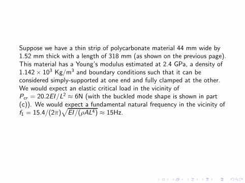
Suppose we have a thin strip of polycarbonate material 44 mm wide by1.52 mm thick with a length of 318 mm (as shown on the previous page).This material has a Young’s modulus estimated at 2.4 GPa, a density of1.142× 103 Kg/m3 and boundary conditions such that it can beconsidered simply-supported at one end and fully clamped at the other.We would expect an elastic critical load in the vicinity ofPcr = 20.2EI/L2 ≈ 6N (with the buckled mode shape is shown in part(c)). We would expect a fundamental natural frequency in the vicinity off1 = 15.4/(2π)

√

EI/(ρAL4) ≈ 15Hz.

Using these two values to normalize the measured (tensile) axial loadsand the measured fundamental frequencies we obtain the data pointsshown in the figure. Similar tests on struts of other lengths andthicknesses can also be suitably nondimensionalized and the resultsconfirm the almost linear (stiffening) effect of the (tensile) loads on thesquare of the natural frequencies. It should be mentioned here that in apractical testing situation there is likely to be a little membrane effect dueto finite amplitude oscillations as well as possible friction at the pinnedend. This is especially the case when the axial loading is compressive.

Energy-based approximate analyses

In using conventional beam theory in a previous section, we made thestandard assumption that the bending moment and curvature werelinearly related (through the flexural rigidity EI ). This allowed a relativelysimple analytic solution to be found. However, a number of approximatetechniques have been developed which are relatively easy to apply, can beused in somewhat more complicated situations including large deflections,e.g., in the post-buckled regime.

If we do not restrict ourselves to small deflections and curvatures it canbe shown that the curvature ψ is related to the lateral deflection via

ψ = w′′

(1 − w′2)−1/2, (22)

where the prime denotes differentiation with respect to the arc length x .It can be shown that this is roughly equivelent to the curvatureexpression more familiar from standard geometry. It can also be shown(based on inextensional beam theory) that the total strain energy storedin bending is

U =1

2EI

∫ L

0

ψ2dx . (23)

Placing ψ in the above expression and expanding, we obtain

U =1

2EI

∫ L

0

(

w′′2 + w

′′2w′2 + .....

)

dx . (24)

Similarly, we can relate the end-shortening to the lateral deflection:

ξ = L−∫ L

0

(1− w′2)1/2dx , (25)

which in turn leads to the potential energy of the load:

VP = −1

2P

∫ L

0

(

w′2 +

1

4w

′4 + .....

)

dx . (26)

Given a form for w these two expressions (24 and 26) can then be addedto the appropriate kinetic energy expression.

We assume a solution (buckling mode) of the form

w = Q(t) sinπx

L, (27)

which can then be used to evaluate the strain and end-shorteningenergies to give

V (Q) = U + Vp = 12EI

(

πL

)4 L2Q

2 + 12EI

(

πL

)6 L8Q

4 + ......

−P(

12

(

πL

)2 L2Q

2 + 12

(

πL

)4 3L32Q

4 + .....)

,

(28)

and a kinetic energy expression

T =1

2m

∫ L

0

w 2dx =1

2m

(

L

2

)

Q2. (29)

where terms including the first nonlinear potential energy contributionhave been retained. For example, if P is greater than the Euler criticalvalue then the potential energy takes the form of two minima separatedby a hill-top, i.e., a twin-well form of potential energy.

Non-trivial equilibrium paths (dV /dQ = 0) are now given by

Λ = 1 +π2

8

(

Q

L

)2

(30)

and again application of the general theory (i.e., ω2 = V11/T11) leads to

(dΛ/dω)p(dΛ/dω)f

= −2 (31)

A similar (but less accurate) analysis can be based on assumedpolynomial buckled and vibration mode shapes. For example, byassuming a simple parabola as the fundamental mode shape we wouldarrive at a natural frequency of 120 (as opposed to π4) and a critical loadof 12 (as opposed to π2). That these values are higher than the exactvalues is typical for Rayleigh-Ritz analysis and is a consequence of thesystem being effectively constrained to take the assumed mode whichtherefore artificially stiffens the structure leading to higher values.

A useful means of estimating the fundamental frequency of vibration canbe based on the fact that the frequency corresponds to a stationary valuein the neighborhood of a natural mode. Using an assumed mode it canbe shown that for an inexact eigenvector we get an eigenvalue that differsfrom the true value to the second order.So far we have focused on directly applied axial loads, but there are anumber of other ways in which induced axial loads occur. If the ends ofthe member are constrained in the axial direction then membrane effectscan occur for deflections which are not especially large.

The period of motion for a given set of initial conditions can be obtainedas a first integration. The energy contributions are

T =1

2m

∫ L

0

(w)2dx (32)

U =1

2EI

∫ L

0

(w ′′)2dx (33)

W =1

2P

∫ L

0

1

2(w ′)2dx , (34)

in which it can be shown that the induced axial load is given by

P = EI2Lr2

∫ L

0 (w′)2dx , (35)

where for a beam of cross sectional area A, and radius of gyration r wehave I = Ar2.

Suppose the ends are simply-supported (but not allowed to movein-plane), then the lowest mode for the linear problem is simply a halfsine wave w = Q(t) sin (πx/L). We are primarily interested in themaximum amplitude of motion Qm, then evaluating the energy terms andadding them we obtain the total energy constant

C =π4EI

mL4Q2

m +π4EI

8mL4r2Q4

m, (36)

which then can be used to obtain the phase trajectory as a function of theinitial conditions (i.e., maximum amplitude). This can be subjected toseparation of variables and integrated (numerically) to obtain the naturalperiod (and hence frequency) as a function of maximum amplitude.

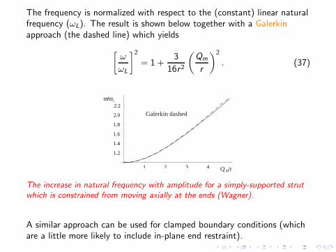
The frequency is normalized with respect to the (constant) linear naturalfrequency (ωL). The result is shown below together with a Galerkinapproach (the dashed line) which yields

[

ω

ωL

]2

= 1 +3

16r2

(

Qm

r

)2

. (37)

1 2 3 4

1.2

1.4

1.6

1.8

2.0

2.2ω/ω L

Q /r

Galerkin dashed

m

The increase in natural frequency with amplitude for a simply-supported strutwhich is constrained from moving axially at the ends (Wagner).

A similar approach can be used for clamped boundary conditions (whichare a little more likely to include in-plane end restraint).

In cases in which appreciable axial loading is present and especially inbuckling it is well established that small geometric imperfections mayhave a profound effect on behavior. In terms of the linear theory, considera simply-supported strut with an initial deflection (i.e., prior to theapplication of any load) of the form w0 = Q0 sin (πx/L. In this case thestatic response is given by

wtotal = w0 + w =

(

Q0

1− α

)

sin (πx/L), (38)

where α = P/PE and PE is the Euler load, and thus, the maximumlateral deflection (at the strut mid-point) is given by

Qmax =Q0

1− α=

Q0

1− PPE

, (39)

i.e., deflections grow unlimited when the elastic critical load for theunderlying geometrically perfect strut is approached.

In terms of the large deflection theory the local form of the potentialenergy in the vicinity of a bifurcation is perturbed to:

V =1

24V c1111Q

4 +1

2V

′c11Q

2λ+ V c1 ǫQ, (40)

where ǫ is a small parameter (which breaks the symmetry). In the case ofa slender strut this small parameter might relate to an initial curvature,axial load offset or small lateral load: they can be shown to have quitesimilar effects on subsequent behavior.

For the continuous strut (with a small initial deflected amplitude of Q0 -representing a half sine wave) the equilibrium paths are given by

Λ = 1 +π2

8

(

Q

L

)2

−(

Q0

L

)(

L

Q

)

, (41)

and the frequency expression is given by

Ω2 = 2(Λ− 1) + 3

(

Q0

L

)(

L

Q

)

, (42)

We see that these degenerate into the perfect case for Q0 = 0.

0

0.2

0.4

0.6

0.8

1

1.2

0 0.1 0.2 0.3

P

Q/L

Q /L=0.050

(a)

0

0.2

0.4

0.6

0.8

1

1.2

0 0.2 0.4 0.6 0.8 1

P

ω2

(b)

(a) Equilibrium paths for a slightly curved axially loaded strut, (b)corresponding frequency-load relation.

We see that since there is no distinct instability the natural frequencysimply reaches a minimum in the vicinity of the critical load for theunderlying perfect system (a super-critical pitchfork bifurcation). Thedifferent dashes in this figure represent levels of initial imperfectionincremented by 0.01 from 0 to 0.05.

In this section we conduct an alternative analysis of a simply supportedstrut. Here, we apply Hamilton’s principle followed by a single modeGalerkin procedure. Again axial load is included in the analysis andmoderately large deflections (corresponding to a degree of stretching) areallowed, i.e., we focus attention again on a system in which nodisplacement or rotation is allowed at the supports.

We state Hamilton’s principle in the form

∫ t2

t1

(δT − δU + δW )dt = 0 (43)

The strain energy consists of bending and stretching terms:

δU =

∫ L

0

[

Nxδ

(

∂u

∂x

)

+ Nx

∂w

∂xδ

(

∂w

∂x

)

+ EI

(

∂2w

∂x2

)

δ

(

∂2w

∂x2

)]

dx .

(44)The kinetic energy is given by

δT =

∫ L

0

m∂w

∂tδ

(

∂w

∂t

)

dx . (45)

and the work done by the external load

δW =

∫ L

0

[

Pδ

(

∂u

∂x

)

+ P∂w

∂xδ

(

∂w

∂x

)]

dx . (46)

Integrating by parts, applying the boundary conditions (pinned supportsat either end) leads to the equation of motion (in the lateral direction) of

mw + EI∂4w

∂x4− ∂

∂x

[

(Nx − P)∂w

∂x

]

= 0 (47)

where the second term consists of axial effects from both the externalapplied load, P , and large deflections, i.e., coupling between bending andstretching, Nx , where Nx is based on a truncation of the end shorteningand given by

Nx =EA

2L

∫ L

0

(

∂w

∂x

)2

dx , (48)

in which A is the cross-sectional area of the member.

The deflection w and distance along the beam x can be scaled in theusual way using

W = w/h ξ = x/L (49)

which enables equation 47 to be rewritten as

∂4W

∂ξ4− 12h

EL2

(

L

h

)4∂

∂ξ

[

(Nx − P)∂W

∂ξ

]

+12mh

E

(

L

h

)4∂2W

∂t2= 0. (50)

We now scale the in-plane loads and time using,

p = P

(

L2

EI

)

(51)

Nξ = Nx

(

L2

EIA

)

(52)

τ = t

√

EI

mL4(53)

leading to the final nondimensional equation of motion

∂2W

∂τ2+∂4W

∂ξ4− ∂

∂ξ

[

(Nξ − p)∂W

∂ξ

]

= 0. (54)

with the stretching-bending coupling from

Nξ = 6

∫ 1

0

(

∂W

∂ξ

)2

dξ. (55)

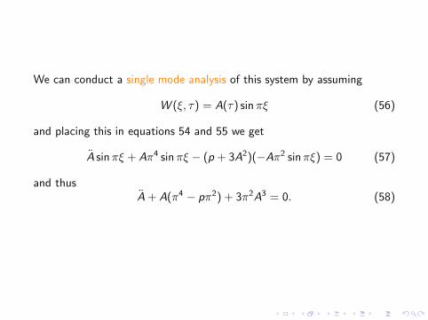
We can conduct a single mode analysis of this system by assuming

W (ξ, τ) = A(τ) sinπξ (56)

and placing this in equations 54 and 55 we get

A sinπξ + Aπ4 sinπξ − (p + 3A2)(−Aπ2 sinπξ) = 0 (57)

and thusA+ A(π4 − pπ2) + 3π2A3 = 0. (58)

This is a cubic (hardening) spring oscillator. Hence we expect to see thestiffening effect due to the immovable ends, even when the deflection isnot especially large. In the absence of axial load, and for small amplitudemotion (such that the cubic term is negligible), we simply have aharmonic oscillation with a frequency of

Ω2n = π4 (59)

which in dimensional terms is the familiar first mode (bending) frequency

ωn = π2

√

EI

mL4(60)

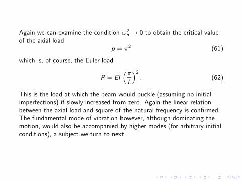
Again we can examine the condition ω2n → 0 to obtain the critical value

of the axial loadp = π2 (61)

which is, of course, the Euler load

P = EI(π

L

)2

. (62)

This is the load at which the beam would buckle (assuming no initialimperfections) if slowly increased from zero. Again the linear relationbetween the axial load and square of the natural frequency is confirmed.The fundamental mode of vibration however, although dominating themotion, would also be accompanied by higher modes (for arbitrary initialconditions), a subject we turn to next.

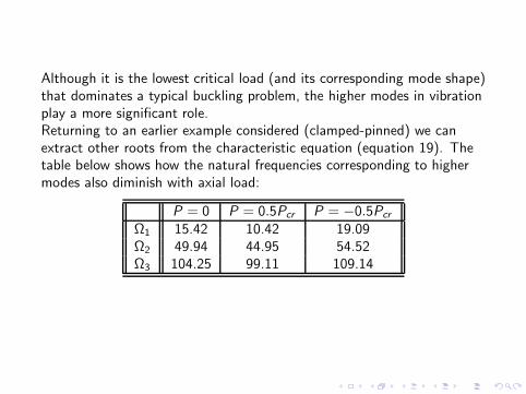
Although it is the lowest critical load (and its corresponding mode shape)that dominates a typical buckling problem, the higher modes in vibrationplay a more significant role.Returning to an earlier example considered (clamped-pinned) we canextract other roots from the characteristic equation (equation 19). Thetable below shows how the natural frequencies corresponding to highermodes also diminish with axial load:

P = 0 P = 0.5Pcr P = −0.5Pcr

Ω1 15.42 10.42 19.09Ω2 49.94 44.95 54.52Ω3 104.25 99.11 109.14

The figure below shows the corresponding mode shapes. Thus we seethat despite a relatively strong influence of axial load on naturalfrequencies, the effect on mode shape is minor (this will not necessarilyto the case for more complicated structures like plates and shells).

0 0.2 0 .4 0 .6 0 .8 1x/L

Second mode

Third mode

The second and third modes for a clamped-pinned strut. The inset shows thecurves in the presence of tensile and compressive axial forces

For the approximate analysis we return to the simply-supported case andadd a second term to the assumed shape:

W (ξ, τ) = A1(τ) sin πξ + A2(τ) sin 2πξ (63)

Using equation 63 to evaluate equations 54 and 55 now leads to the pairof equations

A1 + 3π2A1(A21 + A2

2) + A1(π4 − pπ2) = 0 (64)

A2 + 12π2A2(A21 + A2

2) + A2(16π4 − 4pπ2) = 0, (65)

If we further assume that deflections are small, then we get the secondlowest critical load (p = 4π2) and a second lowest mode of vibration(Ω = 4π4), both of which correspond to a full sine wave. That thelinearized equations are uncoupled is a consequence of the assumedmodes actually corresponding to the normal modes. For a generalstructure this will not typically be the case.

Consider a cantilever strut shown below.

L

m,EIw(x,t)

x

P

Schematic of a cantilevered strut.

In choosing the assumed buckling and vibration modes we wish to have afunction that resembles the true modes as closely as possible. Even for arelatively simple structure (like the cantilever under consideration) thesemodes can be quite complicated. However, it is natural to assume afunction which at least satisfies the geometric boundary conditions.

The cubic polynomial

w(x , t) = C (t)x2 + D(t)x3, (66)

satisfies the conditions of zero displacement and slope when x = 0. Weuse this to evaluate the strain energy in bending

U =1

2

∫ L

0

w ′′2dx = 2EIL(C 2 + 3CDL+ 3D2L2), (67)

the potential energy of the end load

VP = −P1

2

∫ L

0

w ′2dx = −PL3

30(20C 2 + 45CDL+ 27D2L2), (68)

and the kinetic energy

T =1

2m

∫ L

0

w 2dx =m

210(21C 2L5 + 35C DL6 + 15D2L7). (69)

Again, in the vicinity of equilibrium and for linear vibrations we expectthe total potential and kinetic energies to be quadratic functions of thegeneralized coordinates and velocities respectively, and thus

T =1

2Tij qi qj (70)

U + VP =1

2V Eij qiqj , (71)

where use is made of the dummy suffix notation, i.e., any suffix occurringmore than once in a product must be summed over all values.

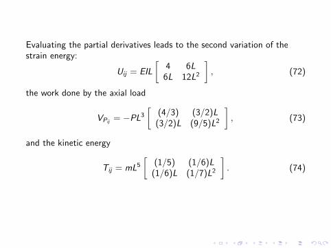
Evaluating the partial derivatives leads to the second variation of thestrain energy:

Uij = EIL

[

4 6L6L 12L2

]

, (72)

the work done by the axial load

VPij= −PL3

[

(4/3) (3/2)L(3/2)L (9/5)L2

]

, (73)

and the kinetic energy

Tij = mL5[

(1/5) (1/6)L(1/6)L (1/7)L2

]

. (74)

We note that these matrices would have been of infinite dimension anddiagonal if the exact mode shapes had been used. We next make use ofthe following definitions

Ω2 =mL4

EIω2, p =

PL2

EI, (75)

and using the characteristic determinantal equation

∣

∣Uij − VPij− ω2Tij

∣

∣ = 0 (76)

we obtain the characteristic equation

12− 5.2p − 0.97Ω2 + 0.05pΩ2 + 0.15p2 + 0.000794Ω4 = 0, (77)

from which we can readily extract the roots.

In the absence of an axial load (p = 0), we have a lowest root ofΩ2 = 12.6. This compares with an exact value of 12.36. By setting thenatural frequency to zero we obtain a lowest root of p = 2.49, whichcompares with the exact value of π2/4. The other roots correspond tothe higher of the two modes, although these are less accurate. It isinteresting to note that using a single generalized coordinate (e.g., withD = 0) leads to a critical load of p = 3 and a natural frequency ofΩ2 = 20.There are a number of ways in which the accuracy of approximatemethods can be improved.

Rotating Beams

An example of slender beams subject to tensile axial loads can be foundin rotor blades. Centrifugal forces due to high rates of rotation typicallylead to stiffening effects. Consider the rotating (cantilever) beam shownbelow.

L

Ω

X

W(X,t)

A rotating cantilever beam.

We can write the governing equation of motion in the usual form

∂2

∂x2

(

EI∂2w

∂x2

)

− ∂

∂x

(

P∂w

∂x

)

+m∂2w

∂t2= 0, (78)

but now the axial load P (in tension) is given by

P =

∫ L

x

mΩ2xdx . (79)

We see that this is similar to equation (13). Separating variables usingw = W (x)Y (t), setting the constant equal to λ2Ω2, we can writeequation (78) (for a uniform beam) in terms of two separated variables

EId4W

dx4− d

dx

(

PdW

dx

)

−mλ2Ω2W = 0, (80)

andd2Y

dt2+ λ2Ω2Y = 0, (81)

and scaling using w = W /L, x = x/L, and ψ = Ωt, we can then write

EId4w

dx4− L2

d

dx

(

Pdw

dx

)

−mλ2Ω2L4w = 0, (82)

andd2Y

dψ2+ λ2Y = 0. (83)

Boundary conditions appropriate for a cantilever beam are zero deflectionand slope at the hub (clamped) end and zero bending moment and shearforce at the free end. Equation (82) can be attacked in a variety of ways,but it is recognized that since the axial force is not a constant (equation79) in this case recourse to approximate solution techniques is required.We have already seen the general influence of tensile axial loads on thenatural frequencies of lateral vibrations. In applications to rotor blades(e.g., in helicopters and turbines) it is interesting to note that a commonconfiguration is to use a hinge at the root of the beam, and hence thesomewhat unusual boundary conditions of pinned-free are encountered.In this case the lowest mode is a rigid body rotation (a flapping motion).The cantilever is often termed a hingeless blade.

Here, we briefly mention a useful approach (related to Rayleigh-Ritz) dueto Southwell. He showed that a relation between the rotating andnon-rotating frequencies could be established as

ω2i = ω2

nr + αiΩ2, (84)

where ωnr is the natural frequency of the non-rotating blade and theSouthwell coefficient αi is given by

αi =

∫ 1

0 mx [∫ x

0 (dwi/dx)2dx ]dx

∫ 1

0mw 2

i dx, (85)

and where wi = wi(x) is an assumed mode shape, satisfying theboundary conditions. Although αi is not strictly constant, the modeshape changes very little with rotation speed.

For Ω → 0 we get the lowest bending mode, which for a pinned-freecantilever is 15.418

√

EI/(mL4), and for a clamped-free cantilever is

3.516√

EI/(mL4). As the rate of rotation gets large we observe anasymptotic relation ωi →

√αiΩ.

For exampleγ = c1γ1 + c2γ2, (86)

in whichγ1(x) = x , γ2(x) = 10x3/3− 10x4/3 + x5. (87)

It is shown that the two roots resulting from this analysis correspond tothe frequencies ω = Ω (flapping motion) and ω = 2.757Ω, and the(normalized) mode shapes plotted:

1Ω

3Ω

2Ω

Ω

ωi

First bending

mode

Rigid body

mode

Ω√

αi

ωnr

mode 1

mode 2

_x

(a) (b)

(a) A ’spoke’ diagram showing the relation between natural frequencies andrate of rotation, (b) The first two mode shapes of a pinned-free rotating beamusing an assumed solution (Bramwell).

Given this basic shape, use can be made of Southwell’s method (equation85), to show how the frequencies change with the speed of rotationaccording to part (a).

Here, we show the table below which summarizes the effect of rotationrate on the lowest three frequencies of clamped-free and pinned-freeuniform cantilevers in which η = Ω/

√

EI/mL4:

η Clamped-free Pinned-free

0 ω1 3.5160 0.000ω2 22.0345 15.4182ω3 61.6972 49.9649

1 ω1 3.6816 1.000ω2 22.1810 15.6242ω3 61.8418 50.1437

3 ω1 4.7973 3.000ω2 23.3203 17.1807ω3 62.9850 51.5498

A considerable amount of research has been conducted on modalinteraction in rotor blades due to elastic and inertial coupling. Clearly,the effects of fluid loading (including forward flight) is complicated, butsuffice it to say here that there are practical situations in which there iselastic coupling between flapping and lagging motion. Southwell’smethod can be applied and flap-lag dynamic interaction obtained. This isan important design consideration for helicopters and stability boundarieshave been developed to take into account the various parameters of theproblem. Given the periodic nature of rotating systems certain specialmathematical techniques can be employed including Floquet theory.

Turbomachinery tends to operate at extremely high rates of revolutionand their blades can experience considerable stiffening effects. Forexample, tip speeds can be close to Mach 1, i.e., a small turbine with aradius of a few centimeters might operate at 100,000 rpm, whereas alarge commercial jet engine might operate in the vicinity of 1,500 rpm.Use is made of Campbell diagrams (also known as waterfall plots andspectrograms) to keep the natural frequencies away from the harmonicsof the rotor speed. Circular plates are sometimes designed so that theirnatural frequencies can be tuned as a function of the rate of spinning.

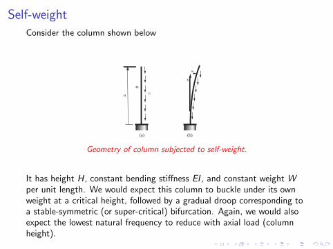
Self-weight

Consider the column shown below

X

w

HG

EI

(a) (b)

Geometry of column subjected to self-weight.

It has height H , constant bending stiffness EI , and constant weight Wper unit length. We would expect this column to buckle under its ownweight at a critical height, followed by a gradual droop corresponding toa stable-symmetric (or super-critical) bifurcation. Again, we would alsoexpect the lowest natural frequency to reduce with axial load (columnheight).

The equilibrium equation is

EIY ′′′′(X ) +W [(H − X )Y ′(X )]′

= 0. (88)

To put the analysis in nondimensional terms, define

a =

(

EI

W

)1/3

, x =X

a, y =

Y

a, h =

H

a. (89)

(The lengths are not nondimensionalized by H, since the height is theparameter of interest.) This leads to the following equation:

y ′′′′(x) + [(h − x)y ′(x)]′

= 0. (90)

The boundary conditions are y(0) = y ′(0) = y ′′(h) = y ′′′(h) = 0. Thecritical nondimensional height is hcr = 1.986.

Approximate values of the critical height can be obtained with the use ofthe Rayleigh-Ritz method as described earlier. The potential energy U isgiven by

U =1

2

∫ h

0

(y ′′)2dx − 1

2

∫ h

0

(h − x)(y ′)2dx . (91)

Making U stationary for the kinematically-admissible function

y(x) = Qxc (92)

where c > 1 leads to the approximate critical height hcr = 2.289 if c = 2,and the value hcr = 2.143 for the minimizing choice c = 1.747. If

y(x) = Q[1− cos(cx/h)], (93)

one obtains hcr = 2.025 for c = π/2 (corresponding to the bucklingmode for a cantilever with axial end load), and hcr = 2.003 for theoptimal value c = 1.829. Finally, the two-term approximation

y(x) = Q1x2 + Q2x

3 (94)

furnishes the excellent approximation hcr = 1.991.

For a circular cross section of radius R we can also use a Rayleigh-Ritzanalysis (based on a simple polynomial displacement function) to obtaincritical height for uniform pole:

hc = 1.26

(

E

ρR2

)1/3

, (95)

in which ρ is the specific weight. For a uniform taper (r = (h − x)R0/h)in which R0 is the radius at the base of the cantilever the coefficient inequation 95 changes to 2.17. It is interesting to note that a rule of taperappropriate for trees (r = ((h − x)/h)3/2R0) the coefficient becomes 2.60so we see a somewhat optimal design in nature (at least in terms ofvertical loading).

A Hanging Beam

A related problem to self-weight buckling is the behavior of long verticalpipes which are subject to axial loads which are not uniform and might,for example, be due to the combined effects of gravity and hydrostaticpressure. A practical example would be the behavior of drill strings in awell bore. Again various end conditions are possible but we shall focusattention on the specific case of a vertical beam, fully fixed at its top endand completely free at the bottom. Hydrostatic pressure is assumed tovary linearly with distance from the top, i.e., a submerged column, andthe effect of gravity is included in the following analysis. At the end ofthis section we will show that for very long and slender beams thebehavior tends towards that of the hanging chain encountered earlier.

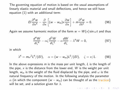
The governing equation of motion is based on the usual assumptions oflinearly elastic material and small deflections, and hence we still haveequation (1) with an additional term:

EI∂4w

∂x4− ∂

∂x

[

(w − wm)x∂w

∂x

]

+m∂2w

∂t2= 0. (96)

Again we assume harmonic motion of the form w = W (x) sinωt and thus

d4W

dζ4− αζ

d2W

dζ2− α

dW

dζ− λ4W = 0, (97)

in which

λ4 = mω2L4/(EI ), α = (w − wm)L3/(EI ), ζ = x/L. (98)

In the above expressions m is the mass per unit length, L is the length ofthe pipe, x is the distance from the lower end, W is the weight per unitlength, wm is the weight of the fluid displaced by the pipe, and ω is thenatural frequency of the motion. In the following analysis the parameterα (in which the component (w − wm) can be thought of as the traction)will be set, and a solution given for λ.

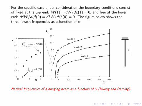
For the specific case under consideration the boundary conditions consistof fixed at the top end: W (1) = dW /dζ(1) = 0, and free at the lowerend: d2W /dζ2(0) = d3W /dζ3(0) = 0. The figure below shows thethree lowest frequencies as a function of α.

0

2

4

6

8

10

12

14

0 200 400 600 800 1000

λ i

α

mode 3

mode 1

mode 2g

λ1

α

λ12 = ω = 3.516

α = 0 1

α = −7.837 λ = 0

Natural frequencies of a hanging beam as a function of α (Huang and Dareing).

It can be shown that the lowest natural frequency (mode 1) drops to zerowhen the traction reaches a level of α = −7.8373, i.e., buckling occurs.In the case of a hanging beam with no hydrostatic pressure but under theaction of gravity alone we can effectively reduce the bending stiffness ofthe system by allowing α to go to very large values, i.e., very largetensions. This tends towards the behavior of a hanging chain, e.g., withα = 1000 we get a lowest natural frequency coefficient tends to 1.22.This compares with the changing chain value of 1.2026 which would havebeen even more closely matched if the upper support were pinned ratherthan fixed.

Experiments

A cantilever under the action of self-weight loading provides a relativelysimple context for experimental verification of some of the behaviordescribed in this section. Consider first a vertically-mounted (built-in endat the bottom), slender elastic rod, of axisymmetric (circular)cross-section, whose length can be increased such that (self-weight)buckling is induced. A cantilever test was conducted whilst the beam wasmounted in a horizontal configuration to determine the flexural rigidity,and this estimate suggested a critical elastic buckling length in thevicinity of 20 cm, based on 1.986(EI/W )1/3. The lateral deflection wasmeasured as a function of height and the results plotted in part (a) of thenext slide. The supercritical nature of the bifurcation is apparent. In part(b) of this figure the lowest natural frequency is also plotted as afunction of height. The minimum is achieved in the vicinity of the criticalheight: it does not drop to zero in practice because of the inevitablepresence of a geometric imperfection (in fact for this type ofaxisymmetric cross section there is no obvious preferred direction forpostbuckled deflection in the perfect case).

0

0.5

1.0

1.5

2.0

2.5

3.0

1.0 1.5 2.0 2.5

h

Lateral tip deflection / a

0 1 2 3 4 5Ω21.50

0

0.5

1.0

1.5

2.0

2.5

3.0

h (a) (b)

(a) Tip deflection and (b) fundamental frequency for a slender rod.

Also, frequencies become increasingly difficult to measure (for smallamplitude vibration) near the buckling length due to the increasing effectof damping. It can also be argued that the damping force has less affectbecause the velocities are decreasing. The postbuckled equilibria andfrequencies (which start to increase in the postbuckling range) can bestudied in the context of an elastica analysis.

Another method of illustrating the effect of gravity is to conduct tests ona double cantilever, i.e., a thin rod clamped at its center point andoriented in the vertical direction. As the rod becomes more slender, thedifference between the upright and downward natural frequenciesbecomes more apparent. A number of thin polycarbonate strips werefabricated such that a range of the nondimensional parameter α (seeequation 98) could be examined. The hub was clamped to anelectro-magnetic shaker and the system subject to a broadband, randomexcitation. A laser vibrometer was then used to acquire velocity datafrom discrete locations along both beams, and subsequent signalprocessing used to obtain frequency response data.

Consider a horizontal polycarbonate strip with cross-sectional dimensionsof 25.4× 4.67 mm, Young’s modulus E = 1.93 GPa, mass per unitlength m = 0.131 kg/m, and length L = 0.737 m.

0.0 20 40 60 80 1000.01

0.1

1

10

Mag

(m/s)/(m/s)

Frequency (Hz)

(a)(b)

A thin prismatic cantilever, (a) experimental configuration, (b) frequencyresponse.

Part (b) showing the superimposed frequency response extracted from 30evenly spaced locations along the entire length. The four lowestmeasured natural frequencies (in Hz) are 1.812, 11.34, 31.71 and 62.35,which compare with analytical values (based on equation 96) of 1.836,11.51, 32.22 and 63.13.

Now, if we take the same system and rotate it 90 degrees we get thefrequency separation (mode splitting) shown below:

0.0 20 40 60 80 1000.01

0.1

1

10

Mag

(m/s)/(m/s)

Frequency (Hz)

100

(a) (b)

0.8 1.2 1.6 2.0 2.4 2.8 3.20.01

0.1

1

10

Mag

(m/s)/(m/s)

100

Frequency (Hz)

Normalized frequency response spectrum for a cantilever in a gravitational field,|α| = 1.23 (a) lowest few frequencies, (b) blow-up of the lowest frequency.

Upon closer inspection each peak is revealed as two adjacent peaks. Forlarger values of α the up or down orientation has a greater effect. Forexample, when we reduce the thickness of the strip to 2.38 mm, and thelength to 0.66 m, while holding everything else constant, we then have|α| = 5.71, and the two peaks separate to approximately 1.65Hz and1.95Hz.

For the upright cantilever we have the result that buckling occurs whenα = −7.837, and the trivial equilibrium loses its stability. Thus, theresults just shown (for which |α| = 1.23) correspond to a cantileverwhose length is (1.23/7.837)1/3 = 55% of its buckling length.We show the results graphically below for both analytical andexperimental frequencies versus α. The lowest frequency, as expected,drops to zero when |α| = −7.837.

100

101

102

103

104

105

0

5

10

15

20

25

30

35

40

Ω2

α| | downward

upright

,

,

α = 0

The four lowest frequencies vs. |α|.

Thermal Loading

We briefly consider the situation in which the axially load is producedthrough a thermal gradient. We start by looking at a simply-supportedbeam which is not allowed to move axially at its ends (and thusgenerating axial forces). If the beam, with coefficient of linear thermalexpansion α is subject to a constant thermal load, the governingequation of motion becomes

mw + EIw IV + AE (αT )w II = 0, (99)

and thus we obtain a natural frequency which is a function of thetemperature change:

ω2 =(π

L

)4(

EI

m

)

[

1− (αT )

(

L

ρπ

)2]

(100)

where ρ =√

I/A is the radius of gyration.

In the absence of a temperature gradient we recover the naturalfrequency of a regular simply-supported beam. Again we have a naturalfrequency that drops to zero as the critical buckling temperature isapproached, but increases if the beam is cooled:

Tcr =(ρπ

L

)2 1

α(101)

Of course, this solution depends on the ends of the beam being preventedfrom moving, but we basically obtain Euler buckling. The issue ofthermal loading is a very complicated one especially for non-simplestructures and non-uniform heating.

Beam on an Elastic Foundation

P K, EI, m

L

A schematic of a thin elastic beam restrained by a linearly elastic foundation.

It is not uncommon for a beam to have some kind of continuous supportalong its length. We can think of this as an elastic foundation, andassume the foundation stiffness is linear. A practical example of thismight be the sleepers under a railroad track, where a significant axialloading effect is caused by thermal expansion. Referring to the schematicshown in the above figure, and again assuming the ends of the beam arepinned, we can extend the analysis from earlier.

The incorporation of a linear elastic foundation results in additional strainenergy stored in the foundation

UK =1

2K

∫ L

0

w 2dx (102)

=1

2K

∫ L

0

q2i sin2 iπx

Ldx (103)

=1

2Kq2i

L

2. (104)

Therefore, we obtain the natural frequencies

ω2i =

1

m

[

EI

(

iπ

L

)4

+ K − P

(

iπ

L

)2]

. (105)

Clearly we recover the results from earlier when we set K = 0, butdepending on the stiffness of the elastic foundation we see the possibilityof a frequency other than the first (corresponding to a half sine wave)dropping to zero first under the action of increasing P .

Introducing the following nondimensional parameters

Ω2 =ω2

EIm

(

πL

)4 , p =P

EI(

πL

)2 , k =K

EI(

πL

)4 , (106)

we obtain nondimensional equations for each mode

1 + k − p = Ω2 : i = 1,

16 + k − 4p = Ω2 : i = 2,

81 + k − 9p = Ω2 : i = 3, (107)

and so on. Without the elastic foundation we observe the familiarrelation between the axial load and the square of the natural frequency.However, the elastic foundation has an interesting effect on the criticalloads, e.g., we see that when k = 4 the lowest two buckling loads are thesame (p = 5). For 4 < k < 36, the critical value of p is 4 + (k/4) andthe corresponding mode has two half-sine waves. In general, if(n − 1)2n2 < k < n2(n + 1)2, the critical value of p is n2 + k/(n)2 andthe governing buckling mode has n half-sine modes.

Suppose we fix k = 12. The relationships in equations (107) are plottedbelow:

0

2

4

6

8

10

12

14

0 20 40 60 80 100

i = 1i = 2i = 3

p

Ω2

k = 12

The interaction of axial load and natural frequencies for a pinned beam restingon a foundation with stiffness k = 12.

For this specific foundation stiffness we have (in the absence of axialloads) frequencies Ω2

1 = 13,Ω22 = 28,Ω2

3 = 93. The lowest three bucklingloads (i.e., when the lowest natural frequency is zero) arep2 = 7, p3 = 10.33, p1 = 13. We see how these modes have changedorder.

Elastically Restrained Supports

It may happen that the actual boundary conditions do not correspondexactly to the classification of pinned, fixed, etc. In this case elasticsprings can be incorporated into the analysis such that when the torsionalstiffness is set equal to zero we obtain the pinned or simply-supportedcase, and when it is infinite we have the fully fixed boundary condition.This allows for a range of intermediate values that can be used to reflectvarying degrees of partial restraint.

Since the elastic end constraints only affect the boundary conditions westill have the familiar equation governing the small amplitude, harmonic,transverse vibrations of a beam given by

d4W

dx4+ p

d2W

dx2− Ω2W = 0, (108)

in which

W = w/L, x = x/L, p = PL2/EI , Ω2 = ρAω2L4/EI . (109)

Again, the solution is given by

W = C1 sinhαx + C2 coshαx + C3 sinβx + C4 cosβx , (110)

withα2 =

√

(p2/4) + Ω2 + p/2

β2 =√

(p2/4) + Ω2 − p/2.(111)

Note the similarity between equations (111) and (15), with the slightdifference due to the definition of nondimensional load used in equation(16) compared with equation (109).

However, with torsional end constraint the boundary conditions become

W (0) = W (1) = 0d2W /dx2 − σ1dW /dx = 0 at x = 0d2W /dx2 + σ2dW /dx = 0 at x = 1

(112)

whereσ1 = k1L/EI , σ2 = k2L/EI , (113)

and the k ’s are the spring stiffness at the left and right hand ends,respectively.

Application of the above conditions leads to the characteristic equation

[

(α2 + β2)2 + σ1σ2(α2 − β2)

]

sinhα sinβ − (114)

2σ1σ2αβ(coshα cosβ − 1)

+(σ1 + σ2)(α2 + β2)(α coshα sinβ − β sinhα cosβ) = 0. (115)

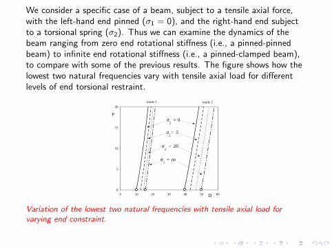
We consider a specific case of a beam, subject to a tensile axial force,with the left-hand end pinned (σ1 = 0), and the right-hand end subjectto a torsional spring (σ2). Thus we can examine the dynamics of thebeam ranging from zero end rotational stiffness (i.e., a pinned-pinnedbeam) to infinite end rotational stiffness (i.e., a pinned-clamped beam),to compare with some of the previous results. The figure shows how thelowest two natural frequencies vary with tensile axial load for differentlevels of end torsional restraint.

0

5

10

15

20

0 10 20 30 40 50 60

P

Ω

mode 1 mode 2

σ2 = 0

σ2 =

σ2 = 20

σ2= 5

oo

Variation of the lowest two natural frequencies with tensile axial load forvarying end constraint.

For zero axial load we observe the frequency coefficients Ω1 = π2 andΩ2 = 4π2 for the pinned-pinned case (i.e., σ2 = 0). The naturalfrequencies increase with tensile force as expected. For pinned-fixedboundary conditions (σ2 = ∞) we obtain the frequencies Ω1 = 15.4 andΩ2 = 50.0. These cases are indicated by the circles. Two intermediatecases are also shown: for σ2 = 5 and σ2 = 20. In those cases in which astructural component makes up one element of a larger structure, orframework, then the actual boundary conditions will typically depend onthe stiffness provided by adjacent members, and this will be the focuslater, when we consider frames.

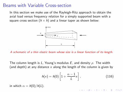
Beams with Variable Cross-section

In this section we make use of the Rayleigh-Ritz approach to obtain theaxial load versus frequency relation for a simply supported beam with asquare cross section (h × h) and a linear taper as shown below:

w(x)

x

L

P

A schematic of a thin elastic beam whose size is a linear function of its length.

The column length is L, Young’s modulus E , and density ρ. The width(and depth) at any distance x along the length of the column is given by

h(x) = h(0)

[

1 +α− 1

Lx

]

, (116)

in which α = h(0)/h(L).

From this, we can compute the area and second moment of area:

A(x) = A(0) [1 + x(α− 1)/L]2

I (x) = I (0) [1 + x(α− 1)/L]4,

(117)

where A(0) = h(0)2 and I (0) = h(0)4/12 are the area and secondmoment of area at the left hand (smaller) end. Given simply-supportedboundary conditions we can assume a half sine wave as the fundamentalmode (we know this is exact for a prismatic beam), i.e.,w(x) = C sinπx/L. The energy expressions for strain energy in bending,potential energy of the loading, and kinetic energy are given by

U =1

2

∫ L

0

EI (x)w ′′2dx (118)

VP =1

2

∫ L

0

Pw ′2dx (119)

T =1

2

∫ L

0

ρA(x)w 2dx . (120)

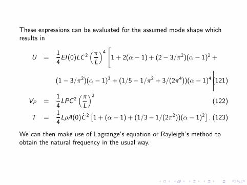
These expressions can be evaluated for the assumed mode shape whichresults in

U =1

4EI (0)LC 2

(π

L

)4[

1 + 2(α− 1) + (2− 3/π2)(α− 1)2 +

(1 − 3/π2)(α− 1)3 + (1/5− 1/π2 + 3/(2π4))(α − 1)4

]

(121)

VP =1

4LPC 2

(π

L

)2

(122)

T =1

4LρA(0)C 2

[

1 + (α− 1) + (1/3− 1/(2π2))(α − 1)2]

. (123)

We can then make use of Lagrange’s equation or Rayleigh’s method toobtain the natural frequency in the usual way.

We note that this result subsumes the case of a prismatic (constant crosssection) beam in which α = 1. However, in general we get

ω2 =

[

1 + 2(α− 1) + 1.696(α− 1)2 + 0.696(α− 1)3 + 0.317(α− 1)4 − p]

[1 + (α− 1)− 0.283(α− 1)2],

(124)where the natural frequency and axial load are nondimensionalizedaccording to

ω2 =ω2

EI (0)/m(πL)4

p =P

EI (0)(πL)2. (125)

For the prismatic beam (α = 1), we get the exact coefficients fromearlier.

The effect of a varying cross section is shown on the next page. Thelinearity of the p vs ω2 relation in part (a) is a consequence of thesingle-mode assumption. By increasing the value of α we are stiffeningthe beam, and hence both the critical load and natural frequencyincrease. For example for a beam whose cross-sectional dimension atx = L is twice that at x = 0, i.e., α = 2 results in a nondimensionalcritical load of approximately 5.47, and a natural frequency (squared) inthe absence of axial load of about 3.3.

0

0.2

0.4

0.6

0.8

1

0 0.5 1 1.5 2 2.5 3 3.5

p

ω2

α = 1

2 . 01 . 8

1 . 61 . 4

1 . 2

_

_ (a)

0

1

2

3

4

5

6

1 1.2 1.4 1.6 1.8 2α

Single-term RR

Six-term RR

Pcr(b)

0.5

1

1.5

2

2.5

3

3.5

4

1 1.2 1.4 1.6 1.8 2

ω2

α

_ (c)

“exact”

(a) The frequency-load relation for various tapered columns; (b) variation of thecritical load with taper (with a sample ’exact’ result for α = 2 superimposed),(c) variation of natural frequency with taper, when the axial load is zero.

The variable cross section does, of course, render the sine wave anapproximate mode shape. More terms in the Rayleigh-Ritz procedure canbe used. The result of using (a very accurate) six terms in just such anexpansion is also shown in the figure as an isolated data point, andspecifically for α = 2 in part (c). As the degree of taper increases thesingle-mode approximation breaks down.

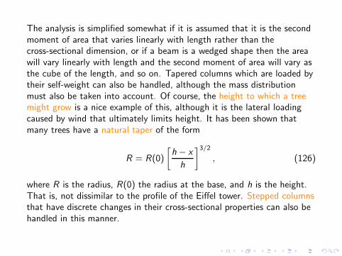
The analysis is simplified somewhat if it is assumed that it is the secondmoment of area that varies linearly with length rather than thecross-sectional dimension, or if a beam is a wedged shape then the areawill vary linearly with length and the second moment of area will vary asthe cube of the length, and so on. Tapered columns which are loaded bytheir self-weight can also be handled, although the mass distributionmust also be taken into account. Of course, the height to which a treemight grow is a nice example of this, although it is the lateral loadingcaused by wind that ultimately limits height. It has been shown thatmany trees have a natural taper of the form

R = R(0)

[

h − x

h

]3/2

, (126)

where R is the radius, R(0) the radius at the base, and h is the height.That is, not dissimilar to the profile of the Eiffel tower. Stepped columnsthat have discrete changes in their cross-sectional properties can also behandled in this manner.