vibration and acoustical properties of sandwich composite
TRANSCRIPT

VIBRATION AND ACOUSTICAL PROPERTIES OF SANDWICH COMPOSITE
MATERIALS
Except where reference is made to the work of others, the work described in this dissertation is my own or was done in collaboration with my advisory committee.
This dissertation does not include proprietary or classified information.
_________________ Zhuang Li
Certificate of approval:
___________________ __________________________ Subhash C. Sinha Malcolm J. Crocker, Chair Professor Distinguished University Professor Mechanical Engineering Mechanical Engineering ____________________ ___________________________ George T. Flowers A. Scottedward Hodel Professor Associate Professor Mechanical Engineering Electrical Engineering ___________________________ Stephen L. McFarland
Acting Dean Graduate School

VIBRATION AND ACOUSTICAL PROPERTIES OF SANDWICH COMPOSITE
MATERIALS
Zhuang Li
A Dissertation
Submitted to
the Graduate Faculty of
Auburn University
in Partial Fulfillment of the
Requirements for the
Degree of
Doctor of Philosophy
Auburn, Alabama May 11, 2006

iii
VIBRATION AND ACOUSTICAL PROPERTIES OF SANDWICH COMPOSITE
MATERIALS
Zhuang Li
Permission is granted to Auburn University to make copies of this dissertation at its discretion, upon request of individuals or institutions and at their expense.
The author reserves all publication rights.
______________________________ Signature of Author
______________________________ Date of Graduation

iv
VITA
Zhuang Li, son of Shouan Li and Shuxian Hao, was born on September 4, 1975, in
Shijiazhuang, Hebei Province, China. He graduated from the Middle School Attached to
Hebei Normal University in 1994. He entered Tianjin University, Tianjin, China in
September 1994, and graduated with two Bachelor of Engineering degrees in Precision
Instrument Engineering and Industrial Engineering in July 1998. He continued his study
in Tianjin University in September 1998, and obtained Master of Engineering degree in
Precision Instruments and Machinery in March 2001. He entered Graduate School,
Auburn University, in August 2001. He married to Yan Du, daughter of Xingrun Du and
Fengqin Liu, on December 25, 2002.

v
DISSERTATION ABSTRACT
VIBRATION AND ACOUSTICAL PROPERTIES OF SANDWICH COMPOSITE
MATERIALS
Zhuang Li
Doctor of Philosophy, May 11, 2006 (M.E., Tianjin University, 2001) (B.E., Tianjin University, 1998)
203 Typed Pages
Directed by Malcolm J. Crocker
In applications where the use of lightweight structures is important, the introduction
of a viscoelastic core layer, which has high inherent damping, between two face sheets,
can produce a sandwich structure with high damping. Composite sandwich structures
have several advantages, such as their high strength-to-weight ratio, excellent thermal
insulation, and good performance as water and vapor barriers. So in recent years, such
structures have become used increasingly in transportation vehicles. However their
fatigue, vibration and acoustic properties are known less. This is a problem since such
composite materials tend to be more brittle than metals because of the possibility of
delamination and fiber breakage. Structures excited into resonant vibration exhibit very
high amplitude displacements which are inversely proportional to their passive damping.
The transmission loss of such composite panels is also poor at coincidence. Their passive

vi
damping properties and attempts to improve their damping at the design stage are
important, because the damping properties affect their sound transmission loss, especially
in the critical frequency range, and also their vibration response to excitation.
The research objects in this dissertation are polyurethane foam-filled honeycomb
sandwich structures. The foam-filled honeycomb cores demonstrate advantages of
mechanical properties over pure honeycomb and pure foam cores. Previous work
including theoretical models, finite element models, and experimental techniques for
passive damping in composite sandwich structures was reviewed. The general dynamic
behavior of sandwich structures was discussed. The effects of thickness and delamination
on damping in sandwich structures were analyzed. Measurements on foam-filled
honeycomb sandwich beams with different configurations and thicknesses have been
performed and the results were compared with the theoretical predictions. A new modal
testing method using the Gabor analysis was proposed. A wavelet analysis-based noise
reduction technique is presented for frequency response function analysis. Sound
transmission through sandwich panels was studied using the statistical energy analysis
(SEA). Modal density, critical frequency, and the radiation efficiency of sandwich panels
were analyzed. The sound transmission properties of sandwich panels were simulated
using AutoSEA software. Finite element models were developed using ANSYS for the
analysis of the honeycomb cell size effects. The effects of cell size on both the Young’s
modulus and the shear modulus of the foam-filled honeycomb core were studied in this
research. Polyurethane foam may produce a negative Poisson’s ratio by the use of a
special microstructure design. The influence of Poisson’s ratio on the material properties
was also studied using a finite element model.

vii
ACKNOWLEDGMENTS
The Author would like to express his sincere appreciation and thanks to his advisor
Professor Malcolm J. Crocker for his guidance during the studies. All the committee
members provided considerable assistance for which I am grateful. My appreciation also
goes to my friends and colleagues at Auburn University. Last and not least, I want to
express my special thanks to my parents Shouan Li and Shuxian Hao, and my wife Yan
Du, for their support and love.

viii
Journal used: Journal of Sound and Vibration
Computer software used: Microsoft Word 2002

ix
TABLE OF CONTENTS
LIST OF TABLES . . . . . . . . xii
LIST OF FIGURES . . . . . . . . xiii
CHAPTER 1 INTRODUCTION. . . . . . . 1
1.1 Sandwich Composite Materials . . . . . 1
1.2 Motivation for Research . . . . . . 4
1.3 Organization of Dissertation . . . . . 6
CHAPTER 2 LITERATURE OVERVIEW . . . . . 12
2.1 Overview of Damping . . . . . . 12
2.1.1 Damping mechanisms . . . . . 13
2.1.2 Measures of damping . . . . . 15
2.1.3 Measurement methods . . . . . 16
2.2 Damping in Sandwich Structures . . . . . 17
2.2.1 Analytical models . . . . . 18
2.2.2 Damping and damage . . . . . 26
2.2.3 Finite element models . . . . . 27
2.2.4 Statistical energy analysis method . . . 29
CHAPTER 3 ANALYSIS OF DAMPING IN SANDWICH MATERIALS . 40
3.1 Equation of Motion . . . . . . 41
3.2 Effects of Thickness . . . . . . 46

x
3.3 Effects of Delamination . . . . . . 51
3.4 Damping Improvement using Multi-layer Sandwich Structures . 51
3.5 Experiments . . . . . . . 55
3.5.1 Experimental setup . . . . . 55
3.5.2 Experimental results . . . . . 56
3.5.3 Discussion . . . . . . 57
CHAPTER 4 DAMPING CALCULATION AND MODAL TESTING . 74
USING WAVELET AND GABOR ANALYSES
4.1 Wavelet and Gabor Analyses . . . . . 75
4.2 Modal Extraction using Wavelet Analysis . . . 79
4.3 Damping Calculation using Gabor Analysis . . . 82
4.3.1 Decouple modes using Gabor analysis . . . 83
4.3.1 Damping calculation . . . . . 85
4.3.2 Simulations . . . . . . 86
4.3.3 Comparison with FFT-based technique . . . 88
4.4 Modal Testing using Gabor Transform . . . . 89
4.5 Experiments . . . . . . . 92
4.5.1 Experimental setup . . . . . 92
4.5.2 Natural frequency and mode shape . . . 93
4.5.3 Damping ratio . . . . . . 93
CHAPTER 5 ANALYSIS OF SOUND TRANSMISSION THTROUGH . 110
SANDWICH PANELS
5.1 Review of the Sound Transmission Loss of Sandwich Panels . 111
xi
5.2 Prediction of Sound Transmission through . . . 115
Sandwich Panels using SEA
5.2.1 Modal density . . . . . . 119
5.2.2 Analysis of critical frequency . . . . 120
5.3 Experimental Results and Discussion . . . . 122
5.3.1 Transmission loss measurement using two-room method 122
5.3.2 Transmission loss measurement using sound intensity method124
5.3.3 Radiation efficiency . . . . . 125
5.3.4 Simulation using AutoSEA . . . . 126
5.3.5 Experimental and simulation results . . . 127
CHAPTER 6 ANALYSIS OF FOAM-FILLED HONEYCOMB . . 144
CORES USING FEM
6.1 Size Effect on the Young’s Modulus . . . . 145
6.2 Size Effect on the Shear Modulus . . . . . 148
6.3 Influence of Poisson’s Ratio . . . . . 150
6.4 More Considerations of Cell Size Effects . . . . 152
CHAPTER 7 CONCLUSIONS . . . . . . 164
REFERENCES . . . . . . . . 169
APPENDICES .. . . . . . . . 179
APPENDIX A MATLAB PROGRAMS FOR WAVENUMBER . 180
AND WAVE SPEED OF SANDWICH PANELS
APPENDIX B MATERIAL PROPERTIES OF SANDWICH PLATES 183
NOMENCLATURE . . . . . . . . 184

xii
LIST OF TABLES
Table 2.1. Formulas used to calculate the loss factor by different methods . 17
Table 3.1. Configurations of intact beams . . . . . 59
Table 3.2. Configurations of beams with delamication . . . 59
Table 4.1. Detected natural frequencies and damping ratios for simulated . 95
signals with different noise level
Table 4.2. Damping ratios of two-mode decay signal calculated using . 95
Gabor expansion
Table 4.3. Damping results calculated using the Gabor spectrogram method 96
Table 4.4. Comparison of the SNRs of the signals reconstructed using . 96
the FFT method and the Gabor expansion method
Table 4.5. Error analysis of the new modal testing method . . . 97
Table 4.6. Damping ratios calculated using the Gabor expansion method . 97
and the Gabor spectrogram method
Table 5.1. Geometry parameters of panels under study. . . . 130
Table 5.2. Reverberation times of the receiving room with different panels . 131
Table 6.1. Cell size effect on the Young’s modulus of foam-filled . . 153
honeycomb beams
Table 6.2. Influence of aspect ratio on the shear modulus calculation using FEM 154
Table 6.3. Cell size effect on the shear modulus of foam-filled honeycomb beams 155

xiii
LIST OF FIGURES
Figure 1.1. Corrugation process used in honeycomb manufacture . . 9
Figure 1.2. Fabrication of foam-filled honeycomb sandwich panels . . 10
Figure 1.3. (a) Polyurethane foam-filled paper honeycomb core . . 11
(b) Built-up sandwich beam with carbon fiber face sheets
Figure 2.1. The effect of the shear modulus on the total damping . . 33
in a sandwich structure
Figure 2.2. The effects of the shear and structural parameters . . 34
on the system loss factor
Figure 2.3. The frequency dependence of the damping in sandwich structures 35
Figure 2.4. The shear parameter effect on the total damping . . 36
in multi-layer sandwich beams
Figure 2.5. A sandwich beam with a spacer beneath the damping layer . 37
Figure 2.6. Variation of modal loss factor with the normalized shear modulus 38
Figure 2.7. Internal damping treatment . . . . . 39
Figure 3.1. A symmetric sandwich beam . . . . . 60
Figure 3.2. Dispersion relation for sandwich beams with a single . . 61
foam core and a foam-filled honeycomb core
Figure 3.3. The cross section of a five-layer sandwich beam . . . 62
Figure 3.4. A beam with 50.8 mm delaminations on both sides . . 63

xiv
Figure 3.5. Experimental setup for damping measurements . . . 64
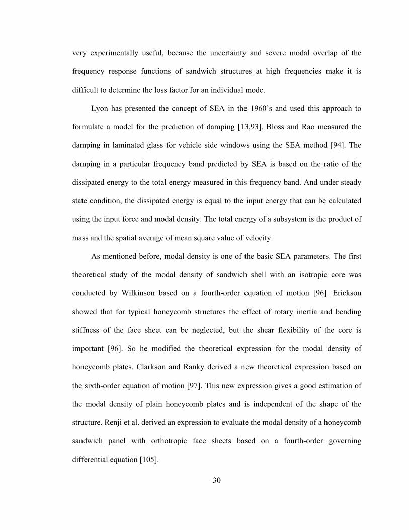
Figure 3.6. Receptance FRFs of beams A and B . . . . 65
Figure 3.7. Comparison of damping ratio in beams A and B . . . 66
Figure 3.8. Receptance FRFs of beams A and C . . . . 67
Figure 3.9. Comparison of damping ratio in beam A and beam C . . 68
Figure 3.10. Receptance FRFs of intact beam A and delaminated beam D . 69
Figure 3.11. Comparison of damping ratio of intact beam A . . 70
and delaminated beam D
Figure 3.12. Damping ratios of beams with delamination only on one side . 71
Figure 3.13. Damping ratios of beams with delaminations on both sides . 72
Figure 3.14. Young’s modulus of sandwich beams as a function of . . 73
delamination length
Figure 4.1 Sampling grids for wavelet transform and Gabor transform . 98
Figure 4.2. (a) An accelerance FRF measured from a sandwich beam . 99
(b) Outline coefficient from the lowpass filter branch of a five-
order standard DWT. (c) Detail coefficients from the high-pass
filter branch of a five-order standard DWT
Figure 4.3. (a) A simulated noisy accelerance FRF with natural frequency . 100
of 200 Hz and damping ratio of 2%. (b) Denoising result from
a five-order undecimated wavelet transform with the calculated
natural frequency of 199.79 Hz and damping ratio 1.99%
Figure 4.4. (a) A free vibration signal measured from an aluminum . . 101

xv
cantilever beam. (b) The wavelet scalogram. (c) The
original Gabor coefficients. (d) The Gabor spectrogram
Figure 4.5. (a) The original Gabor coefficients of signal shown in Fig 4.4 (a) 102
(b) (c) (d) The modified Gabor coefficients of three modes by
using three mask matrices
Figure 4.6. The decoupled modal responses using Gabor expansion . . 103
(a) the first mode, (b) the second mode, (c) the third
mode, and (d) spectra of the three reconstructed signals
Figure 4.7. Damping calculation simulation using the Gabor transform . 104
(a) A simulated free vibration signal, (b) the original Gabor
coefficients of this signal, (c) and (d) the reconstructed
modal responses, and (e) and (f) envelopes established
using the Hilbert transform and the best exponential fits
Figure 4.8. Damping calculation simulation using the Gabor spectrogram . 105
(a) A simulated free vibration signal, (b) the Gabor
spectrogram, (c) and (d) the two vibration modes calculated
using zoom Gabor spectrogram
Figure 4.9. The original complex FFT of a free vibration signal . . 106
containing three modes. (a) Real part, (b) imaginary part
Figure 4.10. Comparison of the envelopes of the displacement . . 107
components reconstructed using the FFT and Gabor expansion
methods. (a) First mode, (b) second mode, (c) third mode
Figure 4.11. Experimental setup for modal testing . . . . 108

xvi
Figure 4.12. Comparison of the theoretical and measured mode shapes . 109
Figure 5.1. Schematic of the power flow in three-coupled systems using SEA 116
Figure 5.2. Modal distribution of isotropic and anisotropic plates . . 132
Figure 5.3. Side views of the two reverberation rooms, and experimental . 133
setup for transmission loss measurements using intensity probe method
Figure 5.4. Comparison of sound transmission loss measurements of . 134
composite Plate A using two-room method and sound
intensity method
Figure 5.5. Sound transmission loss model using AutoSEA software . 135
Figure 5.6. Measured and simulated radiation efficiency of Panel E . . 136
Figure 5.7. Sound transmission loss of Panel E . . . . 137
Figure 5.8. Measured and simulated radiation efficiency of Panel A . . 138
Figure 5.9. Measured and simulated radiation efficiency of Panel B . . 139
Figure 5.10. Measured and simulated sound transmission loss of Panel A . 140
Figure 5.11. Measured and simulated transmission loss of Panel B . . 141
Figure 5.12. Comparison of sound transmission loss and sound transmission 142
class of plates in study
Figure 5.13. Comparison of sound transmission loss and sound transmission 143
class of Plate A and an aluminum plate having the same surface density
Figure 6.1. (a) A section of the honeycomb structure. . . . 156
(b) Beam element used to model the honeycomb cell wall
Figure 6.2. Cell size effect on the Young’s modulus of pure honeycomb structures 157

xvii
Figure 6.3. (a) A section of the honeycomb structure. . . . 158
(b) Beam element used to model the honeycomb cell wall
Figure 6.4. (a) Schematic of the shear modulus calculation. (b) Foam-filled 159
honeycomb finite element mesh and pure shear deformation
Figure 6.5. Honeycomb cell size effect on Young’s modulus and . . 160
shear modulus of foam-filled honeycomb structures
Figure 6.6. Microstructures giving negative Poisson’s ratios . . . 161
Figure 6.7. Influence of Poisson’s ratio on the Young’s modulus . . 162
of foam-filled honeycomb structures
Figure 6.8. Influence of Poisson’s ratio on the shear modulus of . . 163
foam-filled honeycomb structures

1
CHAPTER 1 INTRODUCTION
1.1 Sandwich Composite Materials
Attempts have been made to reduce vibration and its transmission through
structures and mechanical systems for many years. When an unacceptable noise or
vibration problem needs to be solved, it is necessary to understand it completely, for
example, the sources of the noise and vibration, the path along which the energy is
transmitted, its frequency contents, and other related aspects such as thermal insulation,
impact properties, cost, etc. Noise and vibration control methods fall into two categories,
active and passive.
Passive control involves modification of the mass, stiffness and (or) damping of the
system to make it less sensitive to the noise and vibration environments. In passive
control, some structural changes may be made (for example, de-tuning), or some
additional elements, such as double walls, spring isolators, and dampers, may be
introduced. All these elements simply respond to the sound pressures, deflections,
velocities or accelerations which are caused by the other structural components. They do
not require external assistance.
On the other hand, active control systems require an external source of power to
drive the active devices. Although active control systems may be more effective and

2
reliable than passive methods, especially at low frequencies, they are more expensive.
Active systems must be properly maintained, which also increases the cost.
In applications where the use of lightweight structures is important, the introduction
of a viscoelastic damping layer between two face sheets, can produce a sandwich
structure with high damping. Sandwich structures have the additional advantage that their
strength-to-weight ratios are generally superior to those of metals. The core also increases
the thickness of the structure, which leads to an increase in stiffness of the sandwich
structure. The increase in stiffness also reduces the modal density of the structure which
is proportional to 1/ stiffness . Therefore, the total RMS response will be lower with the
reduced number of modes because the total response depends on the number of modes
which are excited.
The ASTM (American Society for Testing and Materials) standards define a
sandwich structure as follows: “a laminar construction comprising a combination or
alternating dissimilar simple or composite materials assembled and intimately fixed in
relation to each other so as to use the properties of each to attain specific structural
advantages for the whole assembly.” (ASTM C 274-99)
Even though the extensive development of sandwich technology has occurred in
the last two or three decades, sandwich construction has been used for more than a
century. Fairbairn was reported to be the first person to describe the principle of
sandwich constructions way back in 1849. The Mosquito fighter-bomber, built by the De
Havilland Aircraft Company in England during World War Two, however, is regarded as
the first major application of sandwich panels. The excellent performance demonstrated
by this airplane instigated new research to improve techniques of fabricating sandwich

3
structures and developing new materials to act as facings and cores. The landing of the
Apollo space vehicle on the Moon in 1969 marked another significant achievement of
sandwich technology. The Apollo capsule was made from a sandwich structure of steel
face sheets and an aluminium honeycomb core which was lightweight and yet strong
enough to sustain the stresses of launch acceleration and landing deceleration [1-3].
Honeycomb cores, which were developed starting in the 1940’s primarily for
aerospace industry, have the greatest shear strength and stiffness-to-weight ratios, but
require special care to ensure adequate bonding of the face sheets to the core since
honoeycomb cores are hollow. The standard hexagonal honeycomb is the basic and most
common cellular honeycomb configuration, and is currently available in many metallic
and nonmetallic materials. Figure 1.1 illustrates the manufacture process, and the L-
(ribbon direction) and W- (transverse to the ribbon) directions of the hexagonal
honeycomb. In this process, adhesive is applied to the corrugated nodes, the corrugated
sheets are stacked into blocks, the node adhesive cured, and sheets are cut from these
blocks to the required core thickness. The honeycomb cores are suitable for both plane
and curved sandwich applications.
Relatively recent developments in high quality cellular foams have greatly
increased the use of sandwich structures. Although cellular foams do not offer such high
stiffness-to-weight ratios as honeycomb cores, they have other important features. For
example, a foam core is solid on a macroscopic level; so it is easier to bond it to the face
sheets. The viscoelasticity of some foam materials leads to higher vibration damping. In
addition, the closed cellular foams make the sandwich structure buoyant and resistant to
water penetration.

4
Nowadays, sandwich structures with different face sheet and core materials are
increasingly used in various applications. Sandwich structures have many advantages
including high stiffness-to-weight and strength-to-weight ratios, high damping capacities,
good thermal insulation properties, excellent water and vapour barrier performance, good
corrosion resistance, and low cost.
1.2 Motivation for Research
Although sandwich structures have significant advantages, they have some less
favorable properties. For example, their high stiffness-to-weight ratio reduces the critical
frequency of a sandwich panel. In addition, because sandwich panels are generally
orthotropic, the critical frequencies, unlike those of metals, are actually situated in a
frequency band instead of at one particular frequency. These features usually result in
poor sound transmission loss over a wider frequency range. Additionally, composite
materials tend to be more brittle than metals. Because of delamination, debonding and
fiber breakage, fatigue in composite materials is of more concern than in metals because
of the sudden catastrophic failure that can occur.
Knowledge of the passive damping of sandwich structures and attempts to improve
their damping at the design stage thus are important. Analytical models for the sound
transmission loss of panels also require knowledge of the damping of the face plates and
core materials which is contributed not only by the material, but also by the panel
boundaries and acoustic radiation. This dissertation concentrates on improving the
damping and sound transmission of sandwich structures.

5
Cores made of both honeycomb and solid viscoelastic materials have been studied
extensively [58,59,100,105-107]. The core used in this dissertation is made of paper
honeycomb filled with polyurethane (PUR) foam. As described before, honeycomb
material is expected to enhance the stiffness of the entire structure, while the foam
improves the damping. In this study, the material for the face sheet is a carbon fiber
reinforced composite. Figure 1.2 shows the manufacturing setup for such foam-filled
honeycomb sandwich plates. Face sheets and cores of different thicknesses are layered in
a vacuum bag according to the configuration design. These laminates are pre-treated with
an adhesive. A vacuum pump is used and results in atmosphere pressure applied to the
whole sample. If heating is required for adhesive curing, the sample with its vacuum bag
can be placed in an oven. Figure 1.3 illustrates a PUR foam-filled honeycomb core and a
built sandwich beam sample.
Jung and Aref have reported that sandwich structures with combined honeycomb-
foam cores have higher damping than those with individual honeycomb or solid
viscoelastic cores [4]. However, Jung and Aref used a static hysteretic damping model, in
which the damping ratio is independent of frequency. Their conclusion is obviously not
valid. In this dissertation the frequency dependence of damping in sandwich beams with
foam-filled honeycomb cores is analyzed, and the effects of thickness of the face sheets
and the core, and delamination on damping have been studied. Most of the earlier models
ignore the bending and extensional effects in the core. However, this assumption is only
valid for soft thin cores. In this dissertation both the bending and shear effects in the core
are considered. In the theoretical modal the shear stresses are continuous across the face
sheet-core interfaces.

6
Besides the analysis of the vibration properties of sandwich constructions as
structural elements, a study of their acoustical properties must also be taken into account
in the initial design stages of aircrafts, automobiles and ships. This is necessary so that
the weight saving advantages produced by composites are not compromised by high
noise transmission, which would require heavy add-on acoustical treatments in later
design stages. In many applications, it is important to know the sound transmission
characteristics of the sandwich panels used in order to minimize the sound transmission
from the engine into the cabin.
A structural element is generally expected to possess high stiffness (high Young’s
modulus). In addition, in order to raise the critical frequency out of the audible frequency
range, a sandwich panel is expected to have a low shear modulus so that shear waves,
rather than bending waves, are dominant at the frequencies of interest. A change of the
honeycomb cell size results in changes of both the Young’s modulus and the shear
modulus of the core. Finite element models were developed to study the size effect of
honeycomb cell.
Experiments were conducted to verify the analytical models presented in this
dissertation, and to qualitatively determine the vibration damping and sound transmission
characteristics. During the experiments, a new damping calculation method based on the
Gabor transform was developed. This method can also be used in modal analysis.
1.3 Organization of Dissertation
This dissertation contains the results of the present investigation into the objectives
already described. The research work was performed in the Sound and Vibration

7
Laboratory of the Department of Mechanical Engineering at Auburn University. The
results reported are divided into six major chapters.
A thorough review of the damping in sandwich structures is given in Chapter 2.
Previous work including theoretical models, finite element models, and experimental
techniques for passive damping in composite sandwich structures is reviewed in this
chapter. The general dynamic behavior of sandwich structures is discussed.
Chapter 3 analyzes the effects of thickness and delamination on damping in
sandwich structures. Measurements on foam-filled honeycomb sandwich beams with
different configurations and thicknesses have been performed and the results were
compared with the theoretical predictions. The stress-strain relationship and damping of a
five-layered sandwich structure are also studied.
Chapter 4 deals with a new modal testing method using the joint time-frequency
analysis. A wavelet analysis-based noise reduction technique is presented for frequency
response function analysis. Additionally, a new damping calculation method was
developed using the Gabor transform and Gabor spectrogram, and is presented in this
chapter.
Chapter 5 is devoted to the study of sound transmission through sandwich panels.
This chapter starts with a brief review of the previous research work on sound
transmission through sandwich panels. Modal density, critical frequency, and the
radiation efficiency of sandwich panels are analyzed. Simulations of the radiation
efficiency and the sound transmission loss were conducted using AutoSEA. Experimental
results are presented as well.

8
Chapter 6 covers the use of finite element models for the analysis of the honeycomb
cell size effect. The finite element models were developed using ANSYS. The effects of
cell size on both the Young’s modulus and the shear modulus of the foam-filled
honeycomb core were studied in this research. PUR foam may produce a negative
Poisson’s ratio by the use of a special microstructure design. The influence of Poisson’s
ratio on the material properties is also presented in this chapter.
The conclusions drawn from this research are given in chapter 7.

Figure 1.1. Corrugation process used in honeycomb manufacture.
9

Figure 1.2. Fabrication of foam-filled honeycomb sandwich panels.
10

11
(a)
(b)
Figure 1.3. (a) Polyurethane foam-filled paper honeycomb core. (b) Built-up sandwich
beam with carbon fiber face sheets.

12
CHAPTER 2 LITERATURE OVERVIEW
2.1 Overview of Damping
The three essential parameters that determine the dynamic responses of a structure
and its sound transmission characteristics are mass, stiffness and damping. Mass and
stiffness are associated with storage of energy. Damping results in the dissipation of
energy by a vibration system. For a linear system, if the forcing frequency is the same as
the natural frequency of the system, the response is very large and can easily cause
dangerous consequences. In the frequency domain, the response near the natural
frequency is “damping controlled”. Higher damping can help to reduce the amplitude at
resonance of structures. Increased damping also results in faster decay of free vibration,
reduced dynamic stresses, lower structural response to sound, and increased sound
transmission loss above the critical frequency.
There is much literature published on vibration damping. ASME published a
collection of papers on structural damping in 1959 [5]. Lazan’s book published in 1968
gave a very good review on damping research work, discussed different mechanisms and
forms of damping, and studied damping at both the microscopic and macroscopic levels
[6]. This book is also valuable as a handbook because it contains more than 50 pages of
data on damping properties of various materials, including metals, alloys, polymers,
composites, glass, stone, natural crystals, particle-type materials, and fluids. About 20

13
years later, Nashif, Jones and Henderson published another comprehensive book on
vibration damping [7]. Jones himself wrote a handbook especially on viscoelastic
damping 15 years later [8]. Sun and Lu’s book published in 1995 presents recent research
accomplishments on vibration damping in beams, plates, rings, and shells [9]. Finite
element models on damping treatment are also summarized in this book. There is also
other good literature available on vibration damping [10-12].
2.1.1 Damping mechanisms
There are many damping mechanisms that convert mechanical energy from a
vibratory system into heat and other energy forms. Basically damping mechanisms fall
into one of the two categories: external and internal.
External damping mechanisms
External damping mechanisms include acoustic radiation damping, Coulomb
friction damping, joint and boundary damping and so on. The dynamic response of a
structure couples with the surrounding fluid medium, such as air, water or other liquid, in
different ways, for example, by the creation of bending and shear waves. The damping
effects of a fluid medium depends on various factors, including the density of the
medium, the sound wave speed and the mass and stiffness characteristics of the structure
itself [7]. The sound radiation of panels has been studied by Lyon, Maidanik, Crocker,
Clarkson, Mead and other researchers [13-17]. For a solid homogenous panel, the
acoustic radiation damping is proportional to the so-called radiation efficiency. For
modes whose natural frequencies are higher than the critical frequency, the acoustic

14
radiation damping is high. At the critical frequency, because the bending wavelength is
the same as the wavelength of sound wave propagating in air, the radiation efficiency as
well as the acoustic damping is greatest. The acoustic radiation damping is generally
small for modes below the critical frequency.
It is worth noticing that some vibration problems benefit from, and others are hurt
by, an increase in the acoustic radiation damping [12]. For example, since the radiation
loss factor of a sandwich structure is normally much higher than its internal loss factor, if
it is excited in a diffuse sound field, then the time-averaged structural vibration levels are
almost independent of the acoustic damping. In addition, since the radiation loss factor is
proportional to the radiation efficiency, which affects the sound transmission loss, an
increase in the acoustic radiation damping leads to a reduction in the sound transmission
loss [15]. For a particular problem, the overall effects of damping and other factors on the
structural response and sound radiation must be considered.
If a structure is made of normal engineering materials, the material damping is
usually smaller than the joint damping. Joint fasteners can be comprised of bolts, rivets,
adhesive layers or line welds. This is minimal at a welded joint because the surrounding
material is virtually continuous. Adhesive bonding layers are thin and bonding materials
are rigid. Therefore, the damping of bonded structures tends to be lower than that of
structures with bolted and riveted joints [12].
Internal damping mechanisms
Internal damping, or material damping, refers to the conversion of vibrational
energy into heat within the volume of the material. Reference [7] tabulates some of the
most important mechanisms including magnetic effects, thermal effects, atomic
15
phenomena and so on. Any real material subjected to stress/strain cycles dissipates
energy. Generally the damping of viscoelastic materials is higher than that of
conventional metals.
High damping is not the only beneficial property for good noise and vibration
control. The additional effects of many other factors such as mass, stiffness, damage
tolerance and so on have to be considered as well. For example, for a joint whose
damping mechanism is Coulomb friction, the occurrence of maximum dry slip damping
may sometimes develop serious corrosion in the interface regions. High damping is
sometimes associated with low stiffness. So the trade-off between the requirements of
low vibration level and strength must be carefully considered during the design stage of
structures [12].
2.1.2 Measures of damping
Basically there are four measures of damping, the loss factor η, the quality factor Q,
the damping ratio ζ , and the imaginary part of the complex modulus. However, they are
related to each other. The loss factor or damping ratio is used in measurements:
φζπ
η tan2212
=′′′
=====EE
CC
QWD
c
. (2-1)
Here D and W are the dissipated and total powers in one cycle of vibration, C and Cc are
the damping coefficient and the critical damping, 'E and "E are the real and imaginary
parts of complex modulus.

16
2.1.3 Measurement methods
Many references present reviews of damping measurements [7,11,18-20].
Generally, there are three sorts of experimental methods. Table 2.1 lists formulas used to
calculate the loss factor with different methods.
Decay rate method
This method can be used to measure the damping of a single resonance mode or the
average of a group of modes in a frequency band. The structure is given an excitation by
a force in a given frequency band, the excitation is cut off, the output of the transducer is
passed through a band pass filter and then the envelope of the decay is observed. The
damping ratio can be calculated from the slope of the envelope of the log magnitude-time
plot.
Modal bandwidth method
With the frequency response function (log magnitude-time plot or Nyquist diagram),
the half-power point method is the most common form used to determine the damping.
This method applies only to the determination of the damping of a single mode.
Power balance method
As mentioned in the previous section, the SEA method is based on the relationship
between the input power and the dissipated power. So the loss factor can be determined
by measuring the input power and the total energy of a modal subsystem.

17
Table 2.1. Formulas used to calculate the loss factor by different methods.
2.2 Damping in Sandwich Structures
A sandwich structure consists of three elements: the face sheets, the core and the
adhesive interface layers. The great advantage of sandwich structures is that optimal
designs can be obtained for different applications by choosing different materials and
geometric configurations of the face sheets and cores. By inserting a lightweight core
between the two face sheets, the bending stiffness and strength are substantially increased
compared with a single layer homogenous structure, without the addition of much weight.
The viscoelastic core has a high inherent damping capacity. When the beam or plate
undergoes flexural vibration, the damped core is constrained to shear. This shearing
causes the flexural motion to be damped and energy to be dissipated. Additionally, the
normal-to-shear coupling between the core and face sheets reduces the sound
transmission. So in recent years, such structures have become used increasingly in
transportation vehicles and other applications. Rao has described the applications of
viscoelastic damping in automotive and aircraft structures [21]. Besides damping
Method Loss factor
Decay Rate Method fDR
3.27=η
Modal Bandwidth Method nf
ff 12 −=η
Power Balance Method 2in
tot
WfW
ηπ
= , where inW Fv= , 2totW M v=

18
treatments used in structures, sandwich glass has been used in automotive side and rear
windows to reduce noise. Nakra has published a series of reviews on vibration control
with viscoelastic materials [22-24]. Trovik has summarized the major uses of constrained
layer damping treatments up to 1980 [25]. A thorough review of work in fiber-reinforced
composite material damping research has been given by Chandra et al. [26].
2.2.1 Analytical models
When a damping layer is attached to a vibrating structure, it dissipates energy by
direct and shear strains. When a solid beam or plate is bending, the direct strain increases
linearly with distance from the neutral axis. So unconstrained damping layers which
dissipate energy mainly by direct strain are attached to the remote surfaces. On the other
hand, the shear stress is the largest at the neutral axis and zero on the free surfaces.
Therefore, constrained layers dissipate energy by shear stress. It has been shown that
shear damping in viscoelastic materials is higher than in typical structural materials. And
the constrained treatment has higher stiffness than unconstrained damping treatment. For
these reasons sandwich composite structures are widely used.
Since the late 1950’s many papers have been published on the vibration of
sandwich structures. The Ross-Ungar-Kerwin model is one of the first theories which
was developed for the damping in sandwich structures [28]-[31]. In Kerwin’s initial study
an analysis was presented for the bending wave propagation and damping in a simply
supported three-layer beam [28]. One of the limitations of this analysis is that the bending
stiffness of the top layer must be much smaller than that of the bottom layer. Ungar
generalized the earlier study and derived an expression for the total loss factor of

19
sandwich beams in terms of the shear and structural parameters [30]. Based on such an
expression, two important conclusions can be drawn. First, if the constraining layer is
thinner than the viscoelastic damping layer, then the system damping has a maximum
value when the shear parameter of the core has an optimal value in the intermediate range,
as shown in Fig. 2.1, where X and Y are the shear and structural parameters, and β is the
damping in the viscoelastic layer. Second, the loss factor has a maximum value when a
three-layer sandwich structure is symmetric about the neutral axis.
Ruzicka summarized earlier research on viscoelastic shear damping mechanisms
and presented structural damping design configurations, especially the so-called “cell-
insert” idea [32,33]. He stated that the loss factor is independent of stress level for pure
viscoelastic materials. He also analyzed the dynamic properties of viscoelastic-damped
structures using a lumped-parameter model which resulted in a number of conclusions
that agree with those obtained from the flexural wave analysis discussed in [28].
The limitations of Kerwin’s model have been avoided in Yu’s theory by using a
variational approach [34]. Yu took into account inertia effects due to transverse,
longitudinal and rotary motions, and considered the combined effects of three loss factors
associated with the shear and direct stresses of the core and the direct stress in the face
sheets. However, Yu only studied the flexural vibration of symmetric sandwich plates.
Sadasivia Rao and Nakra analyzed the damping in unsymmetric sandwich beams and
plates and also included the inertia effects of transverse, longitudinal and rotary motion
[35]. Inclusion of all the inertia effects in the flexural vibration analysis gives three
families of modes in bending, extension and thickness-shear.

20
In extending the work of Kerwin, DiTaranto derived a sixth-order linear
homogeneous differential equation for freely vibrating beams having arbitrary boundary
conditions [36]-[38]. In this model, modes are completely uncoupled, which greatly
simplifies the general forced vibration problem. However, the loss factor calculated using
this equation does not depend on the boundary conditions. This conclusion obviously
cannot be correct. Mead and Markus modified the theory and studied different boundary
conditions in terms of the transverse displacement [39,40]. Using the separable of
variables method, they derived the natural frequencies of sandwich beams and studied the
effects of the shear and structural parameters on damping. The relationship is similar to
the equation derived in [30]. Mead and Markus proved that the loss factor η is much less
sensitive to the change of the shear parameter when the structural parameter Y is large, as
shown in Fig. 2.2. They also showed that the maximum values of the damping are not
very sensitive to the boundary condition, while different boundary conditions shift the
frequency at which the maximum damping occurs.
In another study, Yan and Dowell initially included the effects of face sheet shear
deformation, and longitudinal and rotary inertia [45]. However, from the set of equations
obtained, the longitudinal and rotary terms are neglected by assuming the face sheets to
be very stiff in shear. This procedure results in a fourth-order partial differential equation.
Mead analyzed the damping in symmetric sandwich plates with one pair of opposite
edges simply-supported [41]. He also studied the effect of different boundary conditions
for the other edges and derived a sixth-order equation. Mead compared the difference
between the fourth-order model derived by Yan and Dowell and the sixth-order model
[42,44]. Based on Mead’s sandwich plate model, Cupial and Niziol included the shear

21
deformation of the face layers and rotary inertia and studied simply supported sandwich
plates [47]. The damping calculated using the shear deformation model is somewhat
lower than obtained from Mead’s model. Wang and Chen studied damping in annular
sandwich plates [48].
Since high damping is usually associated with relatively low stiffness and strength,
it is a good idea to increase the stiffness using multi-span sandwich structures. Mead
extended his previous work to periodically supported sandwich plates [43]. The basic
idea is that at a particular frequency, all the displacement and forces at a point in one
periodic element are identical to those at the corresponding point in the adjacent element,
apart from a phase difference which is determined using an iterative technique. The
frequency dependence of damping and the effects of support spacing and shear
parameters on damping were also studied. Rao and He also analyzed damping in multi-
span sandwich beams [49]. Rao and He derived two sixth-order differential equations to
govern the transverse and longitudinal motions for each span using Hamilton’s principle.
The effects of thickness of the face sheets and core, and location of the intermediate
support on the damping were studied for a two-span sandwich beam.
Rao derived a similar equation of motion using Hamilton’s principle [51]. He
presented an extensive study using computer programs to predict the loss factor and
natural frequencies for different boundary conditions in terms of the shear parameter. Rao
also analyzed flexural vibration of short unsymmetric sandwich beams including all the
higher order effects, such as rotary inertia, bending, extensional and shear effects in all
the layers [50]. He compared the loss factor and natural frequencies obtained using this
new model and earlier models. For a beam where the core is thicker than the face sheets,

22
all the models predict identical results, although Rao’s model includes the higher order
effects. This means, for thick core beams, the effects of rotary inertia, extension and shear
in all the layers are insignificant.
All the researchers introduced above, except Yu, have only considered the
contribution of the damping in the viscoelastic core to the total damping in the entire
structure by using the complex form of the shear modulus of the core. An advantage of
the use of the complex shear modulus is that the differential equations only contain the
even order terms. So they are easy to solve. These models are all based on the following
assumptions: (a) the viscoelastic layer undergoes only shear deformation and hence the
extensional energy of the core is neglected; (b) face sheets are elastic and isotropic and
shear energy contributed in them is neglected; and (c) in the facings plane sections
remain plane and normal to the deformed centerlines of the facings. In Reference [44]
Mead conducted a comprehensive study on a comparison of these models.
Instead of only considering the damping in the core, Ungar and Kerwin also
proposed the so-called modal strain energy (MSE) model in order to include the damping
capacities of all the elements. In this model the damping of the material can be
characterized by the ratio of the energy dissipated in each element to the energy stored in
the material [31]. Based on the MSE method, Johnson and Kienholz produced a method
to predict damping in structures with constrained viscoelastic layers by using finite
element analysis [84]. Hwang and Gibson studied damping in composite materials and
structures at both macromechanical and micromechanical levels using the MSE method
[52-55]. They studied the contribution of interlaminar stresses to damping as well [56].

23
The frequency dependence property of viscoelastic damping was first presented by
Lazan [57]. Ruzicka and Mead came to similar conclusions using lumped-parameter
models [32,12]. Mead also studied the influence of the boundary conditions on the
frequency dependence of the loss factor [40]. Nilsson used Hamilton’s principle to derive
a sixth-order differential equation which governs the bending of sandwich beams. He also
studied the dynamic properties of sandwich structures [58,59]. The behavior of a
sandwich structure in the low frequency region is determined by pure bending of the
entire structure. In the middle frequency region, the rotation and shear deformation of the
core become important. At high frequencies, the bending of the face sheets is dominant.
Therefore, if the damping in the core is higher than that in the face sheets, then the
overall damping has a maximum value in the middle frequency range. On the other hand,
if the damping in the core is less than that in the face sheets, then the total damping has a
minimum value in the middle frequency range. Figure 2.3 shows the calculated total loss
factors for three different cases, where the loss factor in the core η2 is set to be 2 % and
the loss factor in the face sheets η1 varies.
The theoretical models discussed so far can be categorized into two classes, fourth-
order models and sixth-order models. Models derived by Mindlin’s theory and
Timoshenko’s theory both lead to a fourth-order differential equation. Mead [42,44], Rao
[50] and Nilsson [59] all show that sixth-order models lead to more accurate results on
the dynamics and damping than fourth-order models. Nilsson states that due to the
frequency dependence of sandwich structure properties, solutions of the fourth-order
differential equation agree well with measurements at low frequency. However, as the
frequency increases, the calculated results disagree strongly with measurements.
24
Besides the three-layer sandwich structures, multi-layer sandwich structures are
also widely studied [60-67]. Grootenhuis showed that the four-layer and five-layer beams
have wider high damping range in terms of the damping layer shear modulus than three-
layer sandwich beams, as shown in Fig. 2.4, where E and G denote the Young’s modulus
and shear modulus, and h is thickness [62]. Asnani and Nakra studied the damping
characteristics of symmetric multi-layer beams with identical viscoelastic and elastic
layers alternatively arranged [64]. They provided three design criteria and analyzed the
effects of the shear parameter and layer thicknesses on the total damping. Alam and
Asnani extended the previous work to multilayer structures with orthotropic damping
layers where each damping layer is constrained between two elastic layers [65-67]. They
considered shear strain in all the layers. But their result does not satisfy continuity of the
shear stress across the interfaces. Bhimaraddi proposed a refined shear deformation
theory in which the shear stresses are continuous across the interfaces [68]. Rao and He
studied several different multilayer configurations using the numerical analysis [69]. Two
more fiber reinforced layers are added on the two free surfaces. The total damping can be
improved by changing the fiber orientation.
Among the multi-layer sandwich structures, special attention has been given to
spaced sandwich structures. In some sandwich panels, a spacer is inserted between the
base plate and the viscoelastic damping layer to magnify the shear strain and enhance the
damping. Since the viscoelastic damping layer is separated from the neutral axis of the
entire structure due to the spacer, the direct stress is increased. To make this
configuration effective, the shear stiffness of the spacer must be much greater than that of
the damping layer so that the shear stress in the damping layer also increases. Ross,
25
Ungar and Kerwin present this idea first in [29], as shown in Fig. 2.5. Nakra and
Grootenhuis derived the equations of motion using Hamilton’s principle [63]. The Two
face sheets are assumed to be perfectly elastic, and the damping layer and spacer are
viscoelastic. Compared with three layer sandwich beams and plates, multi-layer
structures have wider high damping range in terms of the core shear modulus [62,63].
Van Vuure et al. applied the modal strain energy method to model such structures and the
finite element method to calculate the loss factor in each layer [60]. They also studied the
effects of spacer position.
Since many complex structures have joints, the joint damping is also an interesting
phenomenon. Joint fasteners for sandwich composite structures can be bolts, rivets, or
adhesive layers. He and Rao analyzed the damping in adhesively bonded double-strap
joints [70]. The effects of the shear modulus of the damping layer and structural
parameters, such as the damping and constraining layer thicknesses, on the modal loss
factor are studied. If the viscoelastic damping layer is much softer than the constraining
layer, the total loss factor varies little with the shear modulus of the damping layer. In
Fig. 2.6 the normalized shear modulus is defined as the ratio of the core shear modulus to
the face sheet Young’s modulus.
In general, the damping of bonded structures tends to be lower than that of structures
with bolted and riveted joints [12]. Nanda and Behera conducted a theoretical analysis
and experiments for the damping in bolted laminated structures [71]. The damping in
such structures depends on many factors such as the diameter of the bolts, tightening
torque on the bolts, number of layers, and so on.

26
Marsh and Hale presented a different damping configuration, which consists of an
internal shear damping treatment [72]. Such structures are hollow with viscoelastic
damping materials bonded inside the structures. This is very similar to the “cell-insert”
concept presented by Ruzicka [32,33]. Marsh and Hale analyzed the effects of geometry
and mechanical parameters on the damping in such structures. Figure 2.7 illustrates the
internal damping treatment idea.
2.2.2 Damping and damage
Damage is another mechanism which causes increased damping. Prasad and
Carlsson analyzed debonding and crack growth in foam core sandwich beams using the
finite element method [73]. Experiments were carried out with cantilever beams and
shear specimens [74]. Luo and Hanagus studied the dynamics of delaminated beams by
using a piecewise-linear spring model to simulate the behavior of delaminated layers
[75]. Delamination introduces friction in the unbounded region of the interface. And the
damping increases with the size of the delamination. Meanwhile, increased damping
leads to lower natural frequencies. This effect is significant in the high frequency range
[76].
Delamination affects the stiffness of sandwich beams as well. For beams with
delamination, the bending stiffness is reduced substantially. If there is delamination on
both sides of the beam, the bending stiffness is reduced more than if there is delamination
only on one side. This conclusion is the same as that resulting from Frostig’s model
which is based on high-order elastic theory [77].

27
It is worth noticing that high damping is not the only criterion for noise and
vibration control. The overall effects of many factors such as mass, stiffness, damage
tolerance and so on have to be considered as well. High damping is usually associated
with relatively low stiffness. So the trade-off between the requirement for low vibration
levels and strength and stiffness must be analyzed during the design stage. Some criteria
for assessing the damping effectiveness can be found in [78].
2.2.3 Finite element models
The complex eigenvalue method and the direct frequency response method are two
conventional methods that can be used to evaluate damping. Lu et al. conducted a series
of research on vibration of damped sandwich structures using the direct frequency
response method [79-83]. However, these two conventional methods are both
computationally expensive. In recent years the modal strain energy method and the
Golla-Hughes-McTavish (GHM) method have come into more common use.
As discussed in the first section, the modal strain energy method was proposed by
Ungar and Kerwin and developed by Johnson using finite element analysis. Although this
is an approximate technique for the prediction of damping, the advantage is that only the
response of undamped normal modes needs to be calculated and the energy distributions
are of direct use to the designer in deciding where to locate damping layers [84]. Veley
and Rao studied the effect of the thicknesses of all the layers, and the amount and the
location of the damping treatment [85]. They claim that an increase in the constrained
layer thickness increases the loss factor. Although an increase in the viscoelastic layer
thickness increases the loss factor of the first mode, it decreases the loss factor of higher

28
modes. Zambrano et al. studied the accuracy of this method for the estimation of the
response of structures using viscoelastic dampers [86]. Plagianakos and Saravanos
presented a new finite element model for sandwich beams involving quadratic and cubic
terms for approximation of the in-plane displacement in each layer [87]. The damping is
calculated using the modal strain energy method. The effects of ply orientation, thickness
and boundary conditions on the damping are analyzed. Shorter used a one-dimensional
finite-element mesh to describe the low order cross-sectional deformation of laminates
and the modal strain energy method to calculate the damping [88]. This finite element
model showed that below a particular frequency only longitudinal, shear and bending
waves are observed, while at high frequencies additional propagating waves appear
which involve the out-of-phase flexural motion of the face sheets, which is called
symmetric motion or dilatational motion by other researchers [131,132,140].
The GHM method is a technique for deriving a viscoelastic finite element from the
commonly-used elastic finite element and for measurements of both frequency domain
and time domain material behavior [89]. Based on this model, Wang et al. analyzed the
vibration characteristics of sandwich plates incorporated with the Galerkin method and
conducted experiments with simply supported and clamped plates [90]. The GHM
method can successfully predict the frequency dependence of the complex shear modulus
in the core.
Chen et al. presented an order-reduction-iteration approach to predict the damping
in sandwich structures [91]. Such a method consists of two steps, the first-order
asymptotic solution of the nonlinear real eigenequation and the order-reduction-iteration
of the complex eigenequation.

29
Nayfeh analyzed five-layered sandwich beams using finite element implementation
of the modal strain energy model [92]. He studied different boundary conditions and
partially covered sandwich beams, the effects of the coupling factor, and ratio between
the stiffnesses of the face sheets and the core.
2.2.4 Statistical energy analysis method
Finite element models are generally only efficient for problems at low and middle
frequencies. Since the size of elements must be considerably smaller than the minimum
wavelength, the required number of elements increases dramatically with frequency
range of interest, as well as the geometry and complexity of structure. The statistical
energy analysis (SEA) or power balance method is attractive at high frequencies where a
deterministic analysis of all resonant modes of vibration is not practical. In SEA model, a
complex structure is virtually divided into coupled subsystems. Energy flows from one
subsystem to others. Based on the assumption of power balance of these subsystems, the
averaged behavior of the whole structure can be predicted. Because SEA calculates the
spatial and frequency averaged response, the SEA model for a complex structure could be
quite simple. Modal density, internal loss factor for each subsystem, and coupling loss
factors between the subsystems are the basic SEA parameters.
Since the SEA model is widely used in sound transmission research and damping is
related to the sound transmission properties, especially at the critical frequency, SEA is
also used in damping estimations. Although this method cannot be applied for
measurement of damping in an individual mode of vibration, it is very practical for the
estimation of damping in a particular frequency band. Actually this feature of SEA is
30
very experimentally useful, because the uncertainty and severe modal overlap of the
frequency response functions of sandwich structures at high frequencies make it is
difficult to determine the loss factor for an individual mode.
Lyon has presented the concept of SEA in the 1960’s and used this approach to
formulate a model for the prediction of damping [13,93]. Bloss and Rao measured the
damping in laminated glass for vehicle side windows using the SEA method [94]. The
damping in a particular frequency band predicted by SEA is based on the ratio of the
dissipated energy to the total energy measured in this frequency band. And under steady
state condition, the dissipated energy is equal to the input energy that can be calculated
using the input force and modal density. The total energy of a subsystem is the product of
mass and the spatial average of mean square value of velocity.
As mentioned before, modal density is one of the basic SEA parameters. The first
theoretical study of the modal density of sandwich shell with an isotropic core was
conducted by Wilkinson based on a fourth-order equation of motion [96]. Erickson
showed that for typical honeycomb structures the effect of rotary inertia and bending
stiffness of the face sheet can be neglected, but the shear flexibility of the core is
important [96]. So he modified the theoretical expression for the modal density of
honeycomb plates. Clarkson and Ranky derived a new theoretical expression based on
the sixth-order equation of motion [97]. This new expression gives a good estimation of
the modal density of plain honeycomb plates and is independent of the shape of the
structure. Renji et al. derived an expression to evaluate the modal density of a honeycomb
sandwich panel with orthotropic face sheets based on a fourth-order governing
differential equation [105].

31
As for experimental methods to determine the modal density of panels and beams,
Lyon and DeJong have described some basic approaches [93]. The mode count is a
straightforward method, which identifies and counts the number of resonance peaks from
the frequency response function. At high frequencies, severe modal overlap makes the
modes are indistinct. Clarkson and Pope developed an experimental technique to
determine the modal density of a lightly damped structure by measuring the spatial
average of the driving point mobility (i ) (i ) / (i )Y V Fω ω ω= , where V and F are the
Fourier transforms of the velocity and force signals [97,98]. Theoretically the real part of
the driving point mobility must be positive. Several papers were published later on to
improve this technique. Ranky and Clarkson demonstrated that the one-third octave
bands are too wide. A more suitable bandwidth is 100 Hz for metal plates, but 500 Hz for
honeycomb plates because the modal density of sandwich structures is relatively low
[99]. Because the measured velocity at the driving point include a non-propagating (near
field) component which is not related to the energy input, the velocity of the driving point
should not be included in the calculation of the spatial average velocity. Clarkson and
Ranky also studied the effect of discontinuities in honeycomb plates, such as circular cut-
outs, added mass and added stiffeners [100]. In order to solve the presence of negative
values in the real part of driving point mobility, Brown presented a three-channel
technique by measuring one more signal s(t) which is the original signal to drive the
power amplifier [101]. The driving point mobility is then calculated as
(i ) (i ) / (i )sv sfY G Gω ω ω= , where G is the cross-spectrum. Brown and Norton suggested a
method to correct the error in mobility calculation introduced by the added mass between
the transducer and the structure [102]. Keswick and Norton studied three different

32
excitation arrangement ways of an impedance head and used the spectral mass method to
correct the measured mobility [103]. Hakansson and Carlsson presented a similar
correction method using a dual-channel FFT analyzer with an unloaded impedance head
[104]. Applying Brown and Norton’s correction method, Renji measured the modal
density of foam-filled honeycomb sandwich panels using an improved input mobility
method by including both the real and imaginary parts [106]. Beyond a particular
frequency, the measured modal density decreases with frequency although the theoretical
results still increase. Renji explains this is because the vibration of the honeycomb cells
that occurs at high frequencies.
Based on the experimental techniques introduced above, the loss factors of
sandwich structures are then also measured [97,99,107]. It is important to notice that the
frequency average loss factor in a frequency band is not the arithmetic average of
individual modal loss factors.
If measurements are made in air, the measured loss factor is basically the total
effect of the internal and acoustic radiation loss factors. Since the coincidence frequency
of a sandwich structure is generally lower than thin metal plates due to both the bending
and shear waves propagating in it, the radiation loss factor could be very significant in the
frequency bands of interest. Clarkson and Brown have shown that the use of the loss
factor measured in air in SEA model can lead to large errors in the estimated response,
because for honeycomb sandwich plates, the acoustic damping is the major component of
the total damping [16,108].

33
Figure 2.1. The effect of the shear modulus on the total damping in a sandwich structure.

34
Figure 2.2. The effects of the shear and structural parameters on the system loss factor.

35
Figure 2.3. The frequency dependence of the damping in sandwich structures. Solid line,
η1 = 1.5 %, η2 = 2 %; dashed line, η1 = 3 %, η2 = 2 %; dotted line, η1 = 6 %, η2 = 2 %.

36
Figure 2.4. The shear parameter effect on the total damping in
multi-layer sandwich beams.
(a)
(b)

37
Figure 2.5. A sandwich beam with a spacer beneath the damping layer.

38
Figure 2.6. Variation of modal loss factor with the normalized shear modulus.

39
Figure 2.7. Internal damping treatment.

40
CHAPTER 3 ANALYSIS OF DAMPING IN SANDWICH MATERIALS
In the recent research, cores made of either honeycomb or solid viscoelastic
material have been studied [58,59,105-107]. The core in this particular study was made of
paper honeycomb filled with polyurethane (PUR) foam. The honeycomb material is
expected to enhance the stiffness of the entire structure, while the foam improves the
damping. Jung and Aref reported that sandwich structures with combined honeycomb-
foam cores have higher damping than those with individual honeycomb or solid
viscoelastic cores [4]. However, Jung and Aref used a static hysteretic damping model, so
damping ratios are independent of frequency. This conclusion is obviously not valid. In
this paper the frequency dependence of damping in sandwich beams with foam-filled
honeycomb cores is analyzed, and the effects of thickness of the face sheets and core, and
delamination on damping are studied. Most of the earlier models ignore the bending and
extensional effects in the core. However, this assumption is only valid for soft thin cores.
In this paper both the bending and shear effects are considered. And the shear stresses are
continuous across the face sheet-core interfaces.
The sixth-order equations of motion for sandwich beams are derived using
Hamilton’s principle. The wavenumber and speed of flexural wave propagating in
sandwich beams are thus studied. The effect of thickness and delamination on damping in
sandwich structures is analyzed. Measurements on honeycomb-foam sandwich beams

41
with different configurations and thicknesses have been performed and the results
compared with the theoretical predictions.
3.1 Equation of Motion
First of all, the bending stiffness of a symmetric sandwich beam can be expressed as
2 2 22 2 2 2
2 2 2
2 22 2
02
3 2 3
0
2 2
2 ,6 2 12
c c cf
c c cf
c cf
c
t t tt
f c ft t tt
t tt
f ct
f f f f c cf c
D Ez dA E z bdz E z bdz E z bdz
E z bdz E z bdz
E t E t d E tb D D D
− +
− − −
+
= = + +
= +
⎡ ⎤= ⋅ + + = + +⎢ ⎥
⎢ ⎥⎣ ⎦
∫ ∫ ∫ ∫
∫ ∫ (3-1)
where b is the width of the beam, tf and tc are the thicknesses of the face sheet and core,
Ef and Ec are the Young’s moduli of the face sheet and core, and cf ttd += . Df is the
bending stiffness of a face sheet about its own neutral axis, D0 is the stiffness of the face
sheets associated with bending about the neutral axis of the entire sandwich, and Dc is the
stiffness of the core. Figure 3.1 shows the beam dimensions and layer configuration.
Considering the shear deformation, the slope of the deflection curve us not equal to
the rotation of the beam cross section. According to Timoshenko’s beam model, the total
curvature due to both the bending and shear is
2
2
d w d ddx dx dx
β γ= + , (3-2)
where w is the total flexural displacement, β and γ are the bending and shear deformation.

42
Next, Hamilton Principle will be used to derive the equations of motion and natural
boundary conditions for sandwich beams.
The total kinetic energy due to translation and rotation has the form
2 2
0 0
1 ( , ) 1 ( , )( ) ( ) ( )2 2
L Lw x t x tT t m x dx J x dxt t
β∂ ∂⎛ ⎞ ⎛ ⎞= +⎜ ⎟ ⎜ ⎟∂ ∂⎝ ⎠ ⎝ ⎠∫ ∫ , (3-3)
where L is the total length of the beam, m(x) is mass per unit length, and J(x) is mass
moment of inertia per unit length. And for a symmetric sandwich beam, we have
( ) (2 )f f c cm x b t tρ ρ= + ,
and 3 2 32
2
2
( ) ( )12 2 12
cf
cf
t t
f f f f c c
t t
t t d tJ x z z dA bρ ρ ρρ
+
− −
⎛ ⎞= = + +⎜ ⎟⎜ ⎟
⎝ ⎠∫ .
The total potential energy contains three parts. The potential energy due to pure
bending of the entire beams, under the bending moment M(x,t), is
2
10 0
1 ( , ) 1 ( , )( , )2 2
L Lx t x tU M x t dx EI dxx x
β β∂ ∂⎡ ⎤= = ⎢ ⎥∂ ∂⎣ ⎦∫ ∫ . (3-4a)
The potential energy due to shear deformation in the core, under the shear force V(x,t), is
22
0 0
1 1( , ) ( , ) ' ( , )2 2
L L
cU V x t x t dx k Gbt x t dxγ γ= =∫ ∫ , (3-4b)
where k’ is the shear coefficient which is 5/6 for a beam with rectangular cross-section, G
is the shear modulus of the core. The third part of the potential energy is due to additional
bending deformation in the two face sheets caused by the shear deformation in the core
2
30
L
fU D dxxγ∂⎛ ⎞= ⎜ ⎟∂⎝ ⎠∫ . (3-4c)

43
Then the total potential energy of a sandwich beam can be obtained by combining the
three expressions above. By also including the external distributed load p(x) as shown in
Fig. 3.1, we have
2 2
2
0 0
1 2 ' ( ) ( )2
L L
f cW D D k Gbt dx p x w x dxx xβ β γ
⎡ ⎤∂ ∂⎛ ⎞ ⎛ ⎞= − + + +⎢ ⎥⎜ ⎟ ⎜ ⎟∂ ∂⎝ ⎠ ⎝ ⎠⎢ ⎥⎣ ⎦∫ ∫ . (3-5)
Applying Hamilton’s Principle, we let
( )2
1
0t
t
T W dtδ + =∫ . (3-6)
From Eq. (3-3) we have
2 2 2
1 1 1
2
1
0 0
2 2
2 20
.
t t tL L
t t t
t L
t
w wTdt m dxdt m dxdtt t t t
wm w J dxdtt t
β βδ δ δ
βδ δβ
∂ ∂ ∂ ∂⎛ ⎞ ⎛ ⎞= +⎜ ⎟ ⎜ ⎟∂ ∂ ∂ ∂⎝ ⎠ ⎝ ⎠
⎛ ⎞∂ ∂= − +⎜ ⎟∂ ∂⎝ ⎠
∫ ∫ ∫ ∫ ∫
∫ ∫ (3-7)
After some calculations, the variation of the second term in W is
2
1
2 2
1 1
2
1
2 2
2 20
3 4 2 3 3 4
3 4 2 3 3 40 0
2 2
2 0
2 ( ) ( )
2 2
2 2
t L
ft
Lt tL
f ft t
tL
f ft
wD w dxdtx x x x
w w wD w dxdt D w dtx x x x x x
w wD dt Dx x x
β δ δβ
β β βδ δβ δ
β βδβ
⎛ ⎞ ⎡ ⎤∂ ∂ ∂ ∂− − −⎜ ⎟ ⎢ ⎥∂ ∂ ∂ ∂⎝ ⎠ ⎣ ⎦
⎡ ⎤⎛ ⎞ ⎛ ⎞ ⎛ ⎞∂ ∂ ∂ ∂ ∂ ∂= − + − + −⎢ ⎥⎜ ⎟ ⎜ ⎟ ⎜ ⎟∂ ∂ ∂ ∂ ∂ ∂⎝ ⎠ ⎝ ⎠ ⎝ ⎠⎣ ⎦
⎛ ⎞∂ ∂ ∂ ∂+ − + −⎜ ⎟∂ ∂ ∂ ∂⎝ ⎠
∫ ∫
∫ ∫ ∫
∫2
1
20
( ) .Lt
t
w dtx x
δ⎛ ⎞ ∂⎜ ⎟ ∂⎝ ⎠
∫
(3-8)
Similarly, the variation of the third term in W is

44
2
1
2
1
2 2
1 1
0
0
2
20 0 0
0
' ( )
' ( ) ( )
' ' '
' '
t L
ct
t L
ct
Lt tL L
c c ct t
Lc c
wk Gdt w dxdtx x
w wk Gdt w w dxdtx x x x
w w wk Gdt w k Gdt w dx dt k Gdt dxdtx x x
k Gdt w k Gdt
β δ δβ
δ δβ β δ βδβ
δ δ δβ
βδ δ
∂ ∂⎛ ⎞ ⎡ ⎤− − −⎜ ⎟ ⎢ ⎥∂ ∂⎝ ⎠ ⎣ ⎦
∂ ∂ ∂ ∂⎡ ⎤= − − − +⎢ ⎥∂ ∂ ∂ ∂⎣ ⎦
⎛ ⎞∂ ∂ ∂= − − +⎜ ⎟⎜ ⎟∂ ∂ ∂⎝ ⎠
+ −
∫ ∫
∫ ∫
∫ ∫ ∫ ∫2 2
1 10 0
' .t tL L
ct t
w dx dt k Gdt dxdtxβ βδβ
⎛ ⎞∂−⎜ ⎟∂⎝ ⎠
∫ ∫ ∫ ∫
(3-9)
Then
2 2 2
1 1 1
2 2
1 1
0 0
2
20 0 0
(3 8) (3 9) ( )
(3 8) (3 9) ( ) .
t t tL L
t t t
Lt tL L
t t
Wdt D dxdt p x wdxdtx x
D D dx dt p x wdxdtx x
βδ δβ δ
β βδβ δβ δ
∂ ∂= − + − + − +
∂ ∂
⎛ ⎞∂ ∂= − − + − + − +⎜ ⎟⎜ ⎟∂ ∂⎝ ⎠
∫ ∫ ∫ ∫ ∫
∫ ∫ ∫ ∫ (3-10)
Substitute (3-7) and (3-10) into (3-6), we have
2
1
2
1
2 2 4 3
2 2 4 30
2 2 3 2
2 2 3 20
3 2
3 2
' 2
' 2
' 2
t L
c ft
t L
c ft
c f
w w ww m k Gdt D p dxdtt x x x x
w wJ D k Gdt D dxdtt x x x x
w ww k Gdt Dx x x
β βδ
β β βδβ β
βδ β
⎡ ⎤⎛ ⎞ ⎛ ⎞∂ ∂ ∂ ∂ ∂− + − − − +⎢ ⎥⎜ ⎟ ⎜ ⎟∂ ∂ ∂ ∂ ∂⎝ ⎠ ⎝ ⎠⎣ ⎦
⎡ ⎤⎛ ⎞∂ ∂ ∂ ∂ ∂⎛ ⎞+ − + + − − −⎢ ⎥⎜ ⎟⎜ ⎟∂ ∂ ∂ ∂ ∂⎝ ⎠ ⎝ ⎠⎣ ⎦
⎛ ⎞∂ ∂ ∂⎛ ⎞+ − − + −⎜⎜ ⎟∂ ∂ ∂⎝ ⎠ ⎝ ⎠
∫ ∫
∫ ∫2 2
1 1
2
1
2
20 0
2
20
2
2 0.
L Lt t
ft t
Lt
ft
wdt D D dtx x x
w wD dtx x x
β βδβ
βδ
⎡ ⎤ ⎡ ⎤⎛ ⎞∂ ∂ ∂+ − + −⎢ ⎥ ⎢ ⎥⎟ ⎜ ⎟∂ ∂ ∂⎝ ⎠⎣ ⎦ ⎣ ⎦
⎛ ⎞∂ ∂ ∂⎛ ⎞+ − =⎜ ⎟⎜ ⎟∂ ∂ ∂⎝ ⎠⎝ ⎠
∫ ∫
∫(3-11)
Therefore, we have the governing equations:
2 2 4 3
2 2 4 3' 2 0c fw w wm k Gdt D p
t x x x xβ β⎛ ⎞ ⎛ ⎞∂ ∂ ∂ ∂ ∂
− + − − − + =⎜ ⎟ ⎜ ⎟∂ ∂ ∂ ∂ ∂⎝ ⎠ ⎝ ⎠. (3-12)
2 2 3 2
2 2 3 2' 2 0c fw wJ D k Gdt D
t x x x xβ β ββ
⎛ ⎞∂ ∂ ∂ ∂ ∂⎛ ⎞− + + − − − =⎜ ⎟⎜ ⎟∂ ∂ ∂ ∂ ∂⎝ ⎠ ⎝ ⎠. (3-13)

45
Also, since wδ , δβ and wx
δ ∂⎛ ⎞⎜ ⎟∂⎝ ⎠
are arbitrary, the last three integrals in (3-11) must equal
to zero to get the natural boundary conditions. At x = 0, L, we have
Assume harmonic solutions ( )j t kxw Ae ω −= and ( )j t kxBe ωβ −= . Substitute them into Eqs. (3-
12) and (3-13), then
2 2 4 3
3 2 2 2
' 2 ( ' 2 )( ' 2 ) ' 2 0
c f c f
c f c f
m k Gbt k D k j k Gbt k D k w pj k Gbt k D k J Dk k Gbt D k
ωω β
⎛ ⎞− − + ⎧ ⎫ ⎧ ⎫=⎜ ⎟⎨ ⎬ ⎨ ⎬⎜ ⎟− + − − − ⎩ ⎭ ⎩ ⎭⎝ ⎠
. (3-17)
Since w and β can be arbitrary, the coefficient matrix must be singular. Therefore, by
setting the determinant of the coefficient matrix to zero, we have a sixth-order equation
for the wavenumber k and speed of wave in sandwich beam cb:
( )( )
6 2 4
2 2 2 2 4 2
2 ' 2
2 ' ( ' ) 0.
f f
f
D Dk k GAD D J k
mD mD k GAJ k mJ mk GA
ω
ω ω ω ω ω
+ −
− + + + − = (3-18)
2 2 6 6 4
2 4 2 6
( ' ) ( 2 ' )
( ' 2 ) 2 0.b f b
f b f
m J k GA c m D D k GAJ c
k GAD D J c D D
ω ω ω
ω ω ω
− − + +
+ − + = (3-19)
3 2
3 2' 2c fw wk Gdt Dx x x
ββ⎛ ⎞∂ ∂ ∂⎛ ⎞− = −⎜ ⎟⎜ ⎟∂ ∂ ∂⎝ ⎠ ⎝ ⎠
, or 0w = , (3-14)
2
22 fwD D
x x xβ β⎛ ⎞∂ ∂ ∂= −⎜ ⎟∂ ∂ ∂⎝ ⎠
, or 0β = , (3-15)
2
2
wx xβ∂ ∂=
∂ ∂, or 0w
x∂
=∂
, (3-16)

46
3.2 Effects of Thickness
In the Ross-Ungar-Kerwin model [7,11,30], the loss factor is given by the following
formula
22 )1)(1()2(1 XYXYYX
ββη
+++++= , (3-20)
where
2c
GbX Sk t
= , 2
1 t t b bE I E I SY d
+= ,
bbtt AEAES 11
+= , (3-21)
β is the loss factor of the viscoelastic material, and d is the distance between the neutral
axes of the two face sheets, as shown in Figure 3.1. E, I, A and k represent the Young’s
modulus, moment of inertia, cross-sectional area and wavenumber. X and Y are the shear
and structural parameters, respectively. Subscripts t and b denote the top and bottom face
sheets, and c denotes the core.
Substituting S in the expression for Y, we have
,1
)1(33rrrY
++
= b
t
tt
r = . (3-22)
Differentiating the loss factor with respect to the structural parameter Y gives
0])1)(1()2(1[
)1(21222
22
>+++++
+++=
∂∂
XYXYXXX
Y βββη , (3-23)
which is always positive. That means the loss factor is a monotonically increasing
function of the structural parameter Y.
Setting
0)1(
)(31
213 23
22
3 =⎥⎦
⎤⎢⎣
⎡++
−++
=r
rrrrr
drdY , (3-24)

47
we obtain 1±=r . So when 1=r , the loss factor has a maximum value. Then we can
define t b ft t t= = , where the subscript f stands for the face sheets. In this paper only
symmetric sandwich structures have been studied, as shown in Fig. 3.1.
Similarly, by taking the derivative of the loss factor η with respect to the shear
parameter X, an optimal value of the shear modulus G can be calculated to obtain
maximum damping. That means, in an intermediate range of core shear modulus value,
the beam or plate damping has its highest value.
The material for the face sheet is a carbon fiber reinforced composite. The Young’s
modulus of such a material aggregated with epoxy is 60 GPa, similar to that of aluminum.
So it is very stiff. Paper honeycombs are manufactured by processing paper with resin to
make it water resistant. This produces a low cost core, but one which has very good
mechanical properties. PUR foams have low thermal conductivity and diffusion
coefficients, giving them very good thermal insulation properties. Another advantage of
PUR foams is that they can be produced in finite size blocks as well as in-situ, thus
providing an integrated manufacturing process in conjunction with the manufacture of the
sandwich elements.
We will compare two cases in order to study the effect of the thicknesses of the face
sheets and core on the damping.
1. Since the core is stiff in shear but soft generally, its Young’s modulus is much
smaller than that of the face sheet. By assuming c fE E<< and 02 DDD f +≈ , the
normal stresses in the face sheets and the shear stresses in the core are
11 012
ff
f
MzED D
σ =+
, 1 11
1 012(2 )f f
cf
VE t dD D
τ =+
, (3-25)

48
where M and V are the bending moment and the shear force, respectively.
2. If we assume not only that c fE E<< but also that the face sheets are thin,
f ct t<< , then, 0DD ≈ . The normal stresses in the face sheet and the shear stresses in the
core become
22 2
ff
Mt d
σ = , 22
cVd
τ = , (3-26)
and the normal stresses in the core and the shear stresses in the face sheets are zero. So
the face sheets carry bending moments as tensile and compressive stresses and the core
carries transverse forces as shear stresses.
Comparing the two cases, by assuming they have the same core thickness tc,
bending moment M and shear force V, we have
1 11 1 222 3 2
1 1 1 12 21
12( )
2 6 3
f fc
f f f f fc
E t d d ddE t d E t t
d
ττ
= ⋅ = <+ +
, (3-27)
and
1 2 2 2 22 3 2 3
1 1 1 1 1 12
2 6 2 6
f f f f
f f f f f ff
MzE t d zt dE t d E t t d tM
σσ
= =+ +
.
Since
1 11 1max ( )
2f
f f
d tzσ σ
+= = ± ,
then
2
1
2 2 21 2 1 2 21 1 2 2
33 2 212 2
1 1 11
2 2max (2 )4 233
f c
c
f f f f c c ff f c f
fff f c ff
t t t t t t t t tt t t dt t t t t tt d
σσ
+ + ++= =
+ ++ .

49
Let 1
2
f
f
ta
t= , and
2
c
f
tbt
= , then
21
3 2 22
max 2 2 1, if 1.2474 23
f
f
a ab b b a ba a b ab
σσ
+ + += < < <
+ +. (3-28)
It is easy to prove that Equation (3-28) is a monotonically decreasing function of a and b.
Equations (3-27) and (3-28) show that the thinner the face sheets are, the larger is
the shear in the core and the normal stress in the face sheets. That means, if we increase
the thickness of the face sheets by a factor more than 1.247, the shear in the core is more
constrained. And the direct stress in the face sheets also becomes smaller because the
cross-sectional area is larger.
Consider the dynamic case. Vibration energy can propagate through a sandwich
structure mainly in the form of bending waves and shear waves. Since bending waves
create substantial transverse displacements, bending waves couple best with the
surrounding fluid and are mostly responsible for the sound radiation. However, as shown
before, the shear deformation in the core is significant in sandwich structures in
comparison with homogeneous materials. So shear waves must also be considered. In
Section 3.1 the speed of wave in sandwich beam was derived. Based on Eq. (3-19), Fig.
3.2 compares the variation of the bending wave speed in two sandwich beams with
different core materials. The MATLAB programs, which are used to calculate the speeds
of wave in sandwich structures with isotropic and orthotropic cores, can be found in the
appendices. Case (a) corresponds to a single foam core and case (b) a foam-filled
honeycomb core. The Young’s moduli of the foam core and the foam-filled honeycomb
core are 10.16 MPa and 36.4 MPa. In each plot, the curve Cp represents the speed of

50
wave propagation including the effects of shear deformation. The upper and lower
straight lines depict the pure bending wave speeds of the entire sandwich structure and of
the two face sheets only, respectively. Both the plots demonstrate that at low frequencies,
the wave speed of the sandwich structure is close to the pure bending wave speed in the
entire structure, while at high frequencies, it approaches the speed of the pure bending
wave only propagating in the face sheets. Comparing the two plots, it can be seen that,
for the sandwich beam with a single foam core, the shear deformation is only effective in
the middle frequency range. For a sandwich beam with a foam-filled honeycomb core,
however, the shear deformation is still effective in the high frequency range, because the
honeycomb increases the stiffness of the core.
Therefore, in the low frequency region the energy is dissipated by pure bending
( 0DD ≈ ). With increasing frequency, more energy is dissipated due to the increased
normal-to-shear coupling, in which the motion of the face sheets is mostly transformed
into the shear deformation and in-plane waves in the core. Because of the viscoelastic
property of the foam, the damping in the core is greater than that in the face sheets. Thus
the damping has an increasing trend with frequency.
At high frequencies, if the core is very soft compared with the face sheet, the
bending stiffness of the face sheets about their own neutral axes is dominant and the total
damping is determined by the face sheets ( fDD 2≈ ). That means that the damping
reaches a maximum and decreases again at high frequency [58]. However, for the
material studied, the honeycomb increases the stiffness of the core compared with a core
made only of foam. So the normal-to-shear coupling is still effective in the high
frequency range and thus the damping is increased substantially.

51
Therefore, with an increase in the face sheet thickness, the damping in the low and
high frequency ranges is lower, but it is still high in the middle frequency range. On the
other hand, if the thickness of the core is doubled, the damping is very much increased in
the middle and high frequency ranges.
3.3 Effects of Delamination
Damage is another mechanism which causes increased damping. Delamination
introduces friction in the unbounded region of the interface. And the damping increases
with the size of the delamination. Meanwhile, increased damping leads to lower natural
frequencies. This effect is significant in the high frequency range [76]. In reference [85] a
finite element program developed for a sandwich cantilever beam using NASTRAN
shows that the damping increases with increasing delamination. Our experimental results
presented in this paper are seen to be consistent with this prediction.
Delamination affects the stiffness of sandwich beams as well. The bending stiffness
expression, Eq. (3-1), is derived for undamaged sandwich beams. For beams with
delamination, the integral limits become smaller and the resulting bending stiffness is
reduced substantially. And if there is delamination on both sides of the beam, the bending
stiffness is reduced more than when there is delamination only on one side. This
prediction is the same as Frostig’s model based on high-order elastic theory [77].
3.4 Damping Improvement using Multi-layer Sandwich Structures
Inspired by the basic sandwich effect, an improved high passive-damping sandwich
structure is designed in this chapter. The new structure consists of five layers. Two new

52
viscoelastic layers are inserted between the core and the face sheets, as shown in Fig. 3.3.
The two new layers are expected to introduce more damping into the structure. Since the
Young’s modulus is changed along the z-axis, the bending stiffness of a five-layer beam
can be obtained by using five integrals. For a symmetric structure,
(3-29)
where Ec, Ev, Ef are the Young’s moduli of the core, the viscoelastic layer and the face
sheet, respectively, and b is the width of the beam. The subscripts c, v and f represent the
core, the viscoelastic layer and the face sheet. d1 is the distance between the center lines
of the two viscoelastic layers, cv ttd +=1 . d2 is the distance between the center lines of
the two face sheets, cvf tttd ++= 21 . Df and Dv are the bending stiffnesses of each face
sheet and the viscoelastic layer about their own neutral axes, Df0 and Dv0 are the
stiffnesses of the face sheets and the viscoelastic layers associated with bending about the
neutral axis of the entire sandwich, and Dc is the stiffness of the core.
Therefore, the normal stresses in these layers are:
,22
122266
222
00
321
22
33
2
0
22
2
22
2
2
2
2
22
2
22
2
22
2
22
2
22
cvfvf
ccvvffvvff
t
c
tt
tv
ttt
tt
f
ttt
tt
f
tt
tv
t
tc
t
tt
v
tt
ttt
f
DDDDD
tEdtEdtEtEtEb
bdzzEbdzzEbdzzE
bdzzEbdzzEbdzzEbdzzEbdzzEdAEzD
ccv
c
cvf
cv
cvf
cv
cv
v
c
c
c
c
v
cv
cv
cvf
++++=⎥⎥⎦
⎤
⎢⎢⎣
⎡++++⋅=
++=
+++==
∫∫∫
∫∫∫∫∫∫
+++
+
++
+
+
−
−
−−
−−
−−−

53
fvc
vcf
f ttt
ztt
DzME
++≤<+=22
,σ , (3-30a)
vccv
v tt
zt
DzME
+≤<=22
,σ , (3-30b)
2, cc
ct
zD
zME≤=σ . (3-30c)
Noticing that the shear force xdMVdx
= , by definition, the shear stress in the beam is
2 2 2
2 2 2 2 2 2 ( )f f ft t td d d
x x xxz
z z z
d V V Q zdM Ezdz dz Ezdzdx dx D D Dστ
+ + +
= = = =∫ ∫ ∫ , (3-31)
where Q(z) is the first moment of area. In the core, or 2ctz ≤ , the first moment of area is
22)
4(
2212
22
2
2
2
2 dtEdtEz
tEzdzEzdzEzdzEQ ffvvcc
ttt
tt
f
tt
tv
t
zcc
fvc
cv
cv
c
c
++−=++= ∫∫∫++
+
+
. (3-32)
Similarly, in the viscoelastic layers, for vcc t
tz
t+≤<
22, we have
2)
2)(
2(
22
2
2
2 dtEzt
tzt
tEzdzEzdzEQ ff
vc
vcv
ttt
tt
f
tt
zvv
fvc
cv
cv
+−+++=+= ∫∫++
+
+
, (3-33)
and in the face sheets, for fvcc tt
tzt
t++≤<+
22,
)2
)(2
(2
2
zttt
ztttE
zdzEQ fvc
fvcf
ttt
zff
fvc
−+++++== ∫++
. (3-34)
Substituting Eqs. (3-32) to (3-34) back into (3-31), then the shear stresses become
,2
x cc c
V tQ zD
τ = ≤ , (3-35.a)

54
,2 2
x c cv v
V t tQ z tD
τ = < ≤ + , (3-35.b)
,2 2
x c cf f v v f
V t tQ t z t tD
τ = + < ≤ + + . (3-35.c)
From Eq. (3-35) we can find that the maximum shear stress occurs at the neutral axis of
the entire beam, when z = 0,
221
0max
8 2 2f fx c c v v
c c z
E t dV E t E t dD
τ τ=
⎡ ⎤= = + +⎢ ⎥
⎣ ⎦ , (3-36)
and the shear stresses are continuous across the interfaces. On the interface between the
core and the viscoelastic layer, the shear stress is
21
2 2 2 2c cf fx v v
t tc vz z
E t dV E t dD
τ τ= =
⎡ ⎤= = +⎢ ⎥
⎣ ⎦, (3-37)
and on the interface between the viscoelastic layer and the face sheet,
2
2 2 2c cv v
f fxt tv fz t z t
E t dVD
τ τ= + = +
= = . (3-38)
On the free surface of the beam, fvc tt
tz ++=
2, from Eq. (3-35.c), the shear stress is
zero.
Comparing Eqs. (3-29), (3-30) and (3-35) and the results derived in Section 3.2, we
can see that the bending stiffness and the stresses in the five-layer structure are all greater
than those of the traditional three-layer sandwich structure. That implies that the insertion
of two thin but highly damped viscoelastic layers will improve the material properties
and the capability to dissipate energy.

55
3.5 Experiments
We studied three intact and six delaminated beams. Their configurations are listed in
Tables 3.1 and 3.2. All the other dimensions of the delaminated beams are the same:
length 609.6 mm, width 25.4 mm, core thickness 6.35 mm and face sheet thickness 0.33
mm. Figure 3.4 illustrates a beam with 50.8 mm delaminations on both sides.
3.5.1 Experimental setup
Figure 3.5 shows the experimental set up for the damping measurements on
sandwich composite beams. The beams were excited with white noise by a shaker
mounted at the middle of the beam. The density of the sandwich material is 278 kg/m3
and the mass of the beam A is 27.33 grams. For such a light structure a general purpose
accelerometer is not applicable, because the effect of mass loading is significant [109].
Therefore a Polytech laser vibrometer was employed to measure the beam response. The
frequency response functions measured by a B&K accelerometer type 4570 shows that
the resonance frequencies are 10% lower measured by the accelerometer than the laser
vibrometer. The B&K PULSE system was used to analyze the signals with the Dual FFT
mode and the damping ratio was determined directly.
At low frequencies, the coherence between the response and force is very poor for
lightweight structures, because the surrounding airflow affects the excitation-response
relationship. So it is difficult to obtain satisfactory measurements for the first mode. One
solution is to excite the structures and to measure the corresponding responses in
extremely narrow frequency bands. In practice both the 3.125 Hz band and the 1.63 Hz
band were used to excite the structures and make measurements using the zoom FFT

56
mode. Since the beams were excited in a very narrow band, in which the excitation
energy was concentrated, the airflow influence is negligible. In that way the coherence
between the force excitation and response was increased up to 0.977.
3.5.2 Experimental results
Figures 3.6 and 3.7 compare the receptance frequency response functions and
damping ratios of beams with single and double-layer face sheets. Double-layer face
sheets add 13% more mass to the beams. Figure 3.6 shows that the vibration properties
do not change very much. However, from Fig. 3.7 we can see that, as expected, the
damping in beam B is lower than that in beam A (see Table 3.1) in the low and high
frequency ranges, because the thicker face sheets constrain the deformation of the core in
beam B more than in beam A. However, in the middle frequency range, the damping ratio
reaches its maximum value.
Figures 3.8 and 3.9 compare the receptance frequency response functions and
damping ratio in beams A and C. The density of the core is 156 kg/m3. So a core which is
twice as thick adds 56% more mass to the beam. Then the natural frequencies shift
dramatically to lower frequencies. And the damping increases, especially in the middle
and high frequency ranges.
Figures 3.10 and 3.11 show the receptance frequency response functions and
damping ratio of the intact beam A and the delaminated beam D. From Fig. 3.11 we can
see that the effect of delamination is more obvious in the high frequency range. The
damping increases as the mode number increases.

57
Figures 3.12 and 3.13 show the damping ratios of the delaminated beams. With 5%
delamination, the damping of each mode increases evenly. With 10% delamination, the
damping ratio of the second mode is seen to be very high. With 20% delamination, both
the first and the second modes have very high damping. Beams with delaminations on
both sides have more damping than those with delamination only on one side.
The fundamental frequency of a cantilever beam is given by
41 25160.3
mLEIf
π= , (3-39)
where m is the mass per unit length and L is the length of the beam. Then the equivalent
Young’s modulus can be obtained by measuring the fundamental frequencies of the intact
and delaminated sandwich beams. Figure 3.14 shows the effect of delamination on the
equivalent Young’s modulus.
3.5.3 Discussion
As discussed before, the system loss factor η reaches a maximum value when the
shear modulus of the core has an optimal value in the intermediate range. In the Ross-
Ungar-Kerwin model, the shear parameter X is inversely proportional to the core
thickness tc. This means that only when the core thickness is also in an optimal range, can
the damping reach a maximum value. He and Rao reported the same prediction using a
numerical simulation [49]. However, the loss factor also depends on the total bending
stiffness which is also affected by the core thickness. Mead proved that the loss factor η
is much less sensitive to the change of the shear parameter X when the structural
parameter Y is large [12]. The shear parameter is then in a much wider range of the

58
optimum value for maximum η. In He and Rao’s study, the core is thinner than the face
sheets and 27Y = . However, for the beams studied in this paper, the face sheets are
much thinner than the cores. So the structural parameter is large as listed in Table 3.1.
In addition, Mead presented the relationship between the maximum loss factor ηmax
and the structural parameter Y:
( )max 22 2 (1 )(1 )Y
Y Yβη
β=
+ + + + . (3-40)
Taking the derivative of ηmax yields:
22
2max
2 2
1[2 2 (1 )(1 )] [1 ](1 )(1 )
[2 2 (1 )(1 )]
Y Y YYd A
dY BY Y
ββ β ββη
β
++ + + + − +
+ += =
+ + + +. (3-41)
The denominator B is always positive. The numerator A:
. (3-42)
So the derivative (3-41) is always positive. This means that the loss factor increases
monotonically with increasing value of Y, if other parameters are fixed. The theoretical
analysis given in Section 3.2 and the experimental results presented in this paper agree
with Mead’s prediction.
22 2
2 2
2
1[2 2 (1 )(1 ) 1 ]1
[2 2 (1 )(1 ) (1 )(1 )]
[2 (1 )(1 )] 0
A Y YY
Y Y
Y
ββ β β
β β β
β β
+> + + + − − +
+
= + + + − + +
= + + + >

59
Intact
beams
Length
(mm)
Width
(mm)
Core thickness
(mm)
Face sheet
thickness (mm)
Structural
parameter Y
Beam A 609.6 25.4 6.35 0.33 1229
Beam B 609.6 25.4 6.35 0.66 338
Beam C 609.6 25.4 12.7 0.33 4627
Table 3.1. Configurations of intact beams.
Delaminated beams Delamination length (mm)
(percentage of length) Delamination location
Beam D 12.7 (5%) One side
Beam E 12.7 (5%) Both sides
Beam F 25.4 (10%) One side
Beam G 25.4 (10%) Both sides
Beam H 50.8 (20%) One side
Beam I 50.8 (20%) Both sides
Table 3.2. Configurations of beams with delamication.

60
tf
tc
tf
y
z
b
0
Figure 3.1. A symmetric sandwich beam. (a) Side view, (b) cross section.
(b)
L
xd
p(x) z
(a)
60

61
Figure 3.2. Dispersion relation for sandwich beams with a single foam core (a) and a
foam-filled honeycomb core (b).
(a)
(b)
Ec = 10.16 MPa
Ec = 36.4 MPa

62
Figure 3.3. The cross section of a five-layer sandwich beam.
face sheetviscoelastic layer core
tf
tv
b
d1tc
tf
y
z
tv
0 d2

63
Figure 3.4. A beam with 50.8 mm delaminations on both sides.

64
Figure 3.5. Experimental setup for damping measurements.
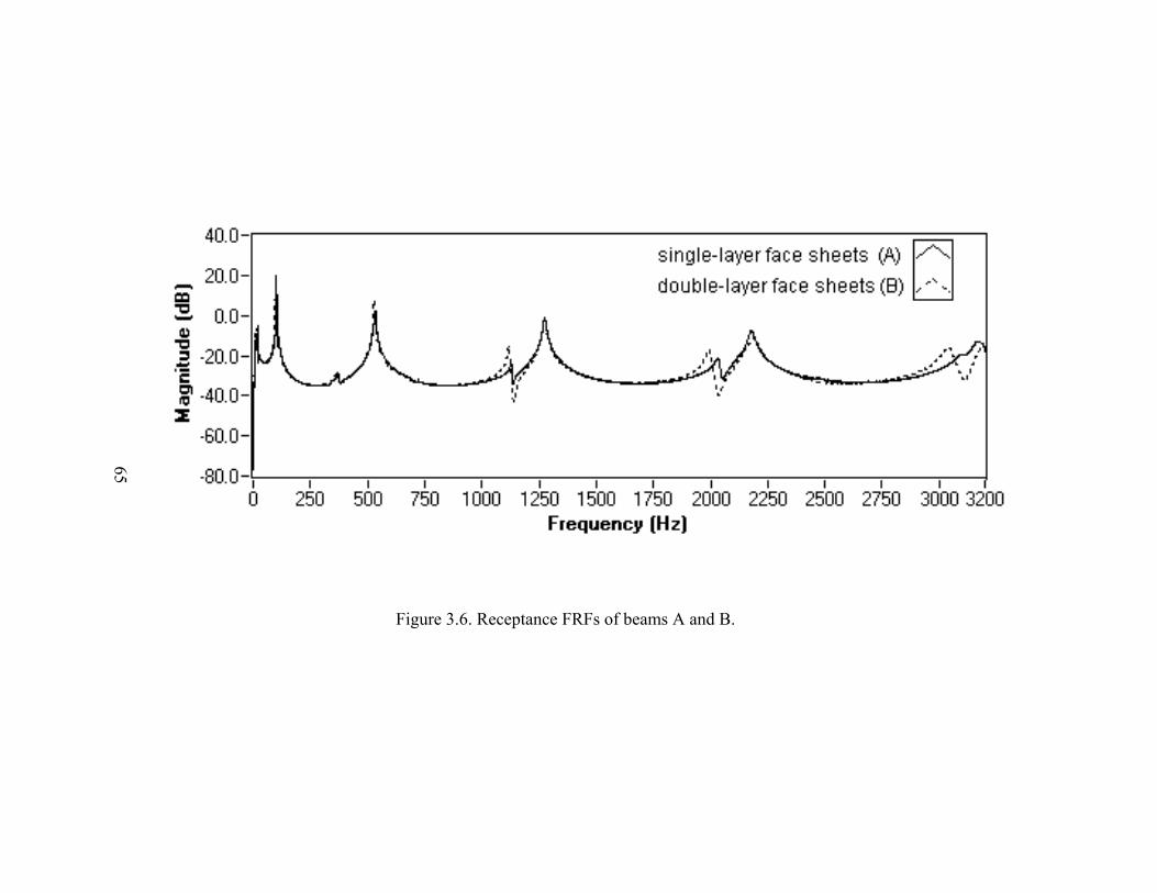
65
Figure 3.6. Receptance FRFs of beams A and B.
65

66
Figure 3.7. Comparison of damping ratio in beams A and B.
66

67
Figure 3.8. Receptance FRFs of beams A and C.
67

68
Figure 3.9. Comparison of damping ratio in beam A and beam C.
68

69
Figure 3.10. Receptance FRFs of intact beam A and delaminated beam D.
69

70
Figure 3.11. Comparison of damping ratio of intact beam A and delaminated beam D.
70

71
Figure 3.12. Damping ratios of beams with delamination only on one side.
71

72
Figure 3.13. Damping ratios of beams with delaminations on both sides.
72

73
Figure 3.14. Young’s modulus of sandwich beams as a function of delamination length.
73

74
CHAPTER 4 DAMPING CALCULATION AND MODAL TESTING USING
WAVELET AND GABOR ANALYSES
Three elementary parameters used in the modal analysis of a dynamic system are its
natural frequency, modal damping and magnitude. A considerable amount of attention
has been devoted to frequency response function (FRF) analysis [20,110,111]. However,
the conventional Fourier analysis approach is restricted to only one domain, because the
elementary functions used to decompose the signals exist from negative infinity to
positive infinity in the time domain. In other words, Fourier analysis cannot provide
information on how the frequency contents of a signal change with time. Therefore,
Fourier analysis is only useful for stationary signals. For non-stationary signals, time-
frequency representations are needed. Consider a simple case, the decay of free vibration.
The decaying vibration signal is non-stationary because its magnitude decreases
exponentially. So it can be viewed as a transient phenomenon. Although it is not difficult
to calculate the loss factor by the decay rate method for lightly damped systems, the
method only works for a single mode at resonance, and the result is very sensitive to
noise. Joint time-frequency analysis (JTAF) can be used instead to separate the modal
components contained in signals and to reduce noise. The modal parameters of each
mode separated thus can be extracted.
Joint time-frequency analysis algorithms fall into two categories: the linear JTFA
and the quadratic JTFA. In the linear JTFA, the short-time Fourier transform (STFT) and

75
the Gabor expansion, which can be regarded as the inverse of the STFT, are two
algorithms. If we consider the linear JTFA as the evolution of the conventional Fourier
transform, the quadratic JTFA is the counterpart of the standard power spectrum.
Quadratic algorithms include the Gabor spectrogram, Cohen’s Class and the adaptive
spectrogram [112-114]. The difference between linear and quadratic JTFA methods is
that the linear transform can be inverted to reconstruct the time signal. Thus, the linear
transform is suitable for signal processing, such as time-varying filtering. However, the
quadratic JTFA describes the energy distribution of the signal in the joint time-frequency
domain, which is useful for signal analysis. Since the phase information is lost in the
quadratic time-frequency representation, the time histories cannot be reconstructed. In
this paper both the linear and quadratic JTFA approaches are used for damping
calculations.
In this chapter the damping calculation and model testing methods using wavelet
and Gabor analyses are studied. This chapter starts with a brief introduction to the
wavelet and Gabor analyses. The modal extraction technique using the undecimated
wavelet-based denoising method in the FRF analysis is then presented in Section 4.2. In
order to decouple the components in a free vibration signal and then calculate the
damping and mode shapes, a new modal testing approach based in the Gabor expansion
was proposed in Sections 4.3 and 4.4.
4.1 Wavelet and Gabor Analyses
Wavelet and Gabor analyses are two sorts of JTFA. The continuous wavelet and
Gabor transforms of a time signal x(t) are defined as

76
∫+∞
∞−
−>==< dt
abttx
axbaCWT ba )()(1,),( *
, ψψ , (4-1)
dtebtgtxgxbCGT tjb
ωωω −+∞
∞−∫ −>==< )(*)(,),( , , (4-2)
where the elementary functions are
)(1, a
bta
ba−
= ψψ , (4-3)
tjb ebtgg ωω )(, −= , (4-4)
and * denotes the complex conjugate.
A comparison of Eqs. (4-1) and (4-2) shows that the wavelet transform and the
Gabor transform are similar except that the elementary functions are different. The
wavelet transform uses the dilated and translated version of the mother wavelet ψ(t) to
decompose the signal, while the Gabor transform uses the modulated and shifted copy of
g(t). Both ψa,b and gb,ω , however, are concentrated at a region of the time-frequency
plane. For example,
),(),( 00
ωω
ωω
tTFtbaCWT === , (4-5)
and
),(),( Ω=Ω== nmTTFnmTbCGT ω . (4-6)
From the two equations above, we can show that the bandwidth of the elementary
functions in the wavelet transform varies with its center frequency, while the bandwidth
of the elementary functions in the Gabor transform does not. This difference leads to the
fact that the time-frequency resolutions of these two transforms are different. According
to the Heisenberg Uncertainty Principle, we cannot obtain high time-resolution and high

77
frequency-resolution simultaneously. The wavelet transform has high time-resolution but
low frequency-resolution at high frequency, and high frequency-resolution but low time-
resolution at low frequency. However, the Gabor transform has a constant time-frequency
resolution once the analysis window is determined [113]. Figure 4.1 compares the
sampling grids of the wavelet transform and the Gabor transform. These features are
appropriate for different applications.
For example, a high-frequency signal lasts for a short time physically. Then it is
necessary to use a function with a high time-resolution to analyze the signal. On the other
hand, a low frequency signal lasts for a long time. Then an elementary function with a
low time-resolution is acceptable. However, this low frequency signal may have a narrow
bandwidth because of the time-scaling property of the Fourier transform. So we need an
elementary function with a high frequency-resolution. Wavelets satisfy such requirements.
For computer applications, numerical wavelet analysis (discrete wavelet transform,
or referred to as DWT) is implemented by filter banks [113,115].
On the other hand, the discrete Gabor transform for a given discrete time sequence
x[k] is computed from
2
, [ ] *[ ]j n k
Nm nC x k k mT e
π
γ−
= −∑ , (4-7)
where Cm,n is a matrix whose entries are called the Gabor coefficients, γ[k] is the analysis
window, and * denotes the complex conjugate. The parameters T and N represent the
discrete time sampling interval and the total number of frequency lines [113]. The
analysis function γ[k] is localized in the joint time-frequency domain. So the Gabor
coefficients will depict the local time-frequency properties of x[k].

78
Random noise is evenly distributed over the entire joint time-frequency domain
because it is not limited to a short time period or a narrow frequency band. On the
contrary, the joint time-frequency representation of a signal is always concentrated in a
relatively small region. After identifying the signal component, a mask can be applied to
filter the signal components and take the inverse transform in order to obtain the noise-
free waveform signal in the time domain.
After computing the Gabor coefficients by Eq. (4-7), a time-varying filter, which is
actually a two-dimensional binary mask function Mm,n, is used to modify the Gabor
coefficient as
, , ,ˆ
m n m n m nC M C= . (4-8)
The component of interest can then be extracted. As long as some requirements are
satisfied, the component in the time domain can be reconstructed as
21 1
,0 0
ˆˆ[ ] [ ]j nkM N
Nm n
m nx k C h k mT e
π− −
= =
= −∑∑ , (4-9)
where h[k] is called the synthesis function [113,116]. Qian had shown that if the
functions h[k] and γ[k] are identical, the Gabor coefficients of the reconstructed signal
ˆ[ ]x k will be optimally close to ,ˆ
m nC , in the sense of least square error. This process is
called orthogonal-like Gabor transformation [113]. In this procedure Eq. (4-7) is called
the Gabor transform (or analysis). And the inverse transform Eq. (4-9) is called the Gabor
expansion (or synthesis).
The Gabor transform is linear JTFA. The quadratic Gabor analysis is called Gabor
spectrogram. Based on the Gabor transform, the Gabor spectrogram is defined as

79
, ', ' , '' '
[ , ] [ , ]D m n m n h hm m n n D
GS i k C C WVD i k− + − ≤
= ∑ , (4-10)
where WVDh,h'[i,k] is the cross Wigner-Ville distribution of the frequency-modulated
Gaussian functions. The order of the Gabor spectrogram, D, controls the degree of
smoothing [114].
4.2 Modal Extraction using Wavelet Analysis
In the modal bandwidth method introduced in Chapter 2, in order to obtain high
coherence between the spectra of acceleration and force and to avoid frequency leakage,
zoom measurement with sufficient frequency resolution was used for each mode. The
maximum frequency resolution of the B&K PULSE system is 6400 lines. However,
because of the fact that the sandwich composite materials have a more complicated
performance than homogenous metals, vibration signals tend to be much noisier. Even
after 400 averages, the frequency response function was not smooth enough with such
high resolution. Figure 4.2 (a) shows a noisy acclerance FRF measured on a sandwich
beam at the resonance frequency of 135 Hz. Since the frequency response function is in
the frequency domain, the general filtering technique does not work. Fortunately, we can
calculate the convolution of the frequency response with a smooth function. Wavelet
analysis is suitable for noise reduction in this situation.
The model for a noisy signal can be expressed as
[ ] [ ] [ ], 0,..., 1x k s k n k k Lσ= + ⋅ = − , (4-11)
where k is the index of the data sample, and L is the length of the data. x[k] is the noisy
signal, s[k] is the true signal we want to recover, n[k] is assumed to be Gaussian white

80
noise, and σ is the noise level. With two-channel filter banks consisting of pairs of
lowpass and highpass filters, the signal is decomposed into low-frequency outline and
high-frequency detail as shown in Fig 4.2 (b) and (c). The small coefficients from the
highpass filter are dominated by noise n[k], while coefficients with high absolute values
carry more signal information s[k] [118]. Replacing the small, noisy coefficients by zero,
we can obtain the essential signal with less noise.
Donoho proposed the wavelet-thresholding denoising method based on the
traditional DWT, or decimation algorithm [119]. This method consists of three stages,
decomposition (referred to as analysis), thresholding detail coefficients, and signal
reconstruction (referred to as synthesis).
After the raw signal is decomposed by multi-resolution analysis (MRA) through
two-channel filter banks at some level, the soft threshold, defined as the fixed form
)log(2 Lt ⋅= , is performed to the detail coefficients from the highpass filter. The soft
thresholding method sets all the detail coefficients with absolute values lower than the
threshold to zero and then shrinks all the other detail coefficients towards zero. The soft
thresholding method has better mathematical properties than the hard thresholding
method. The advantages of the DWT are that the coefficients of the analysis and
synthesis filters do not change at each stage of MRA and the computation complexity
decreases continuously. However, because of decimation, or what is known as
downsampling, for each order, the time-resolution of the signal is much lower than the
raw data. It has to be reconstructed to restore the original time resolution. In Fig. 4.2, (a)
is the raw accelerance frequency response function signal, and (b) and (c) are the output
of the lowpass and highpass filters after the fifth-order MRA, respectively. The wavelet

81
used is biorthogonal with 5th order analysis (decomposition) filter and 3rd order synthesis
(reconstruction) filter, or the so-called bior3_5 wavelet. Because the analysis filter is built
by a fifth-order spline function, the analysis mother wavelet is very smooth. The x-axes
of the plots are the numbers of the data samples. The number of frequency lines of the
raw FRF is 6400. After the fifth-order MRA, the number of frequency lines of the data in
(b) and (c) become 200. That means the time-resolution is 25 = 32 times less than that of
the original signal. So the signal must be reconstructed using the output of each order of
the filter banks to get a smooth curve. It is important to note that the coefficients of the
synthesis filters, which construct the dual filter bank of the analysis filter bank, must
converge. Note that the synthesis using bio3_5 wavelet does not converge although its
analysis effect is very good.
Moreover, as the traditional DWT is translation-variant due to the decimation, the
signal reconstructed from the wavelet coefficients with the nonlinear soft threshold may
also include some distortion. If the maximum point is not at the decimated sample point,
it may be neglected after the thresholding.
An alternative is the so-called A’trous algorithm, or sometimes known as the
undecimated DWT. It uses the same filter banks scheme, but the decomposition is time-
invariant [117]. In other words, the resolution of the signal does not decrease after
decomposition. So it is not necessary to reconstruct the signal. Because of the same
reason, the convergence of the synthesis filters is not required. Another advantage of the
undecimated DWT is that the denoising result has a better balance between the
smoothness and accuracy than the traditional DWT. So the denoising based on the
undecimated wavelet transform is superior to the method using the standard DWT.

82
In order to test the accuracy of the undecimated DWT denoising method, the
following simulation was conducted. The forced response of a single DOF system is
governed by
2( ) 2 ( ) ( ) cosn nx t x t x t F tζω ω ω+ + = ,
where ζ is the damping ratio, ωn is the undamped natural angular frequency, and F is the
force magnitude. Since white noise is used to excite the structure, F is constant in the
frequency range we are interested in. The acceleration magnitude is then
22 2( )
21n n
FA ωω ζωω ω
=⎡ ⎤⎛ ⎞ ⎛ ⎞⎢ ⎥− +⎜ ⎟ ⎜ ⎟⎢ ⎥⎝ ⎠ ⎝ ⎠⎣ ⎦
. (4-12)
Figure 4.3 (a) illustrates a simulated noisy accelerance FRF, where 0.02ζ = ,
0.001F = , the natural frequency fn = 200 Hz, and the standard deviation of the Gaussian
white noise is 0.1. Figure 4.3 (b) shows the denoising result using a five-order
undecimated DWT. The filter coefficients are derived from the bio3_5 wavelet. It can be
seen that the FRF signal is greatly improved. Table 4.1 lists the detected natural
frequencies and damping ratios for different standard deviation levels of the Gaussian
white noise. The numbers in parentheses are relative errors.
4.3 Damping Calculation using Gabor Analysis
In some applications, information about the excitation force is not available.
Although the decay rate method can be used to evaluate the loss factor from a free
vibration signal, as mentioned at the beginning of this chapter, the decay rate method
only works for a single mode at resonance, and the result is very sensitive to noise.

83
Schwarz and Richardson use a curve fitting technique to estimate the modal parameters
from ambient response data [120]. Bonato et al. use Cohen’s class to estimate the modal
parameters from the non-stationary response to an unknown excitation [121]. However,
the algorithms in Cohen’s class, such as the Wigner-Ville Distribution, have cross-term
interferences in the time-frequency representation. References [122] and [123] present a
method for the determination of the logarithmic decrement of free vibration by using the
wavelet scalogram. However, as demonstrated before, the frequency-resolution of the
wavelet transform decreases with increasing frequency. If more than one mode exists in
the vibration decay signal, satisfactory resolution for all modes cannot be obtained. This
is an inherent characteristic of wavelet analysis. In the present research the modal
parameters are estimated using the Gabor expansion and the Gabor spectrogram.
4.3.1 Decouple modes using Gabor analysis
Figure 4.4 (a) illustrates a free vibration signal obtained from the free vibration of an
aluminum cantilever beam. This signal contains three modes at 34.5, 214.4 and 597.5 Hz.
Figure 4.4 (b) is the corresponding wavelet scalogram. As the frequency-resolution is less
in the high frequency range than that in the low frequency range, the vibration components
of the second and third modes are blurred in the scalogram. Even though Lardies has stated
that a modified Morlet wavelet can improve the frequency-resolution, it is indeed a
compromise because the time-resolution is decreased compared to the original Morlet
wavelet. Another problem is that the wavelet scalogram is quadratic, so it cannot be
inverted to reconstruct the time signals. Moreover, since Staszewski and Lardies calculated
the wavelet transform of analytic signals, the computation complexity is twice that of the

84
real signal itself. Finally, the instantaneous frequency components of a real signal and its
corresponding analytic signal may be very different, particularly in the low frequency range
[113].
Unlike the wavelet analysis, the Gabor analysis has a constant time-frequency
resolution once the analysis window is determined. Although such resolution may not be
optimum at a particular point on the time-frequency plane, the Gabor analysis has a
globally optimum time-frequency resolution compared with the wavelet transform, as
shown in Figure 4.4 (c) and (d). In addition, in the present research, in order to avoid the
problems caused by the analytic signal, instead the analytic signal is calculated after
signal reconstruction using the Gabor expansion.
By applying the procedure in Eqs. (4-7) through (4-9) to the Gabor coefficients
shown in Fig. 4.4 (c), the three modes can be reconstructed and the loss factor associated
with each mode thus can be obtained. Figure 4.5 (a) is the same original Gabor
coefficients shown in Fig. 4.4 (c) which is calculated using Eq. (4-7). Three modal
responses at 34.5 Hz, 214.4 Hz and 597.5 Hz can be seen clearly. The color intensity in
the Gabor coefficient plot represents the displacement magnitude which is displayed in
decibels. The noise is distributed in the entire time-frequency domain. By using three
time-varying filters, or actually three mask matrices, the three modal responses can be
decoupled as shown in Figs. 4.5 (b), (c) and (d). A 1024-point optimal Gaussian window
is used to serve as the analysis and synthesis functions in this calculation. The three
decoupled modes thus can be reconstructed using Eq. (4-9). Figure 4.6 illustrates the
reconstructed waveforms and their spectra. It is seen that the property of the signal is
improved significantly and the noise is dramatically reduced. Since each reconstructed

85
waveform becomes a single-mode signal, the natural frequency, magnitude, phase and
damping ratio can also be extracted easily.
Figure 4.4 (d) illustrates the Gabor spectrogram of the same signal shown in Fig.
4.4 (a). The energy distribution of the three modes is clearly seen in the spectrogram.
From this the natural frequencies, damping ratios and magnitude relationships between
these modes can be extracted. However, since the phase information is lost, time histories
cannot be reconstructed from the spectrogram.
4.3.1 Damping calculation
The free response of an underdamped single-degree-of-freedom (DOF) system due
to an impact excitation is given by
( ) cos( )ntdy t Ae tζω ω φ−= − , (4-13)
where ζ is the damping ratio, ωn is the undamped natural angular frequency and the
damped natural angular frequency ωd is
21d nω ω ζ= − . (4-14)
For a small value of damping coefficient ζ, d nω ω≈ . The damping ratio can be
calculated by obtaining the envelope. The traditional decay rate method in which the ratio
of successive peak amplitudes is measured is very sensitive to noise. Another approach to
obtain the envelope is to compute the analytic signal by using the Hilbert transform.
For a given real signal y(t), its analytic signal ( )ay t is
ya(t) = y(t)+jHy(t) , (4-15)

86
where the subscript a stands for analytic, and the Hilbert transform of y(t) is defined as
1 ( ) ( ) yH y t dtτ τ
π τ= −
−∫ . (4-16)
Using Parseval’s formula, we can show that the Fourier transform of Hy(t) is
( ) sgn( ) ( )H j Yω ω ω= − , (4-17)
where sgn(ω) is a sign function, and Y(ω) is the Fourier transform of y(t). So the Hilbert
transform can be easily realized by taking the fast Fourier transform (FFT) of y(t). Then
the magnitude of the vector ya(t) is the envelope of the signal y(t). The damping ratio ζ
associated with each mode can be evaluated by exponential curve fitting from
2e
fζ
πΠ
= − , (4-18)
where Πe is the power of the best exponential fit, and f is the natural frequency extracted
from the reconstructed signal.
4.3.2 Simulations
In order to ensure that the method introduced above result in accurate damping
values, the following simulation was carried out. Figure 4.7 (a) illustrates a simulated free
vibration signal obtained using Eq. (4-19):
0.01 2 200 0.008 2 350( ) sin(2 200 ) 0.85 sin(2 350 ) 0.6 ( )t ty t e t e t n tπ ππ π− ⋅ ⋅ − ⋅ ⋅= ⋅ + ⋅ + + . (4-19)
There are two damped sinusoids, 200 Hz and 350 Hz. Their damping ratios are
chosen to be 0.01 and 0.008, respectively. The noise level n(t) is 0.1. The sampling rate is
1000 Hz and the data length is 300 points. Figure 4.7 (b) shows the Gabor coefficients.

87
By using the Gabor analysis-based time-varying filters, the two simulated modes can be
separated and reconstructed, as shown in Figs. 4.7 (c) and (d). Figures 4.7 (e) and (f)
show the envelopes selected from the decay parts and the corresponding best exponential
fits. The results and the mean squared errors (MSE) are listed in Table 4.2. The numbers
in brackets are the relative errors.
If one is only interested in the damping, and reconstruction is not necessary, the
Gabor spectrogram can also be utilized. Figure 4.8 (a) illustrates the same signal
simulated by Eq. (4-19). Figure 4.8 (b) is the Gabor spectrogram calculated using Eq. (4-
10). The two modes, their frequencies, and the difference between their magnitudes and
damping can be distinguished in this figure. By setting the frequency zoom, we can easily
decouple the modes as shown in Figs. 4.8 (c) and (d).
If the ridges are extracted from the two 3-D plots, then the exponential decay curves
are recovered again. Reference [124] describes several algorithms for ridge detection. An
advanced wavelet application, the so-called ridgelet, has been developed in recent years
[125]. In this research, it is quite simple to recover the decaying vibration signals because
the ridges are concentrated at fixed frequencies.
Unlike the exponential envelope of the signal which can be reconstructed using the
Gabor expansion, the modulation term in Eq. (4-13) is squared because the Gabor
spectrogram calculated using Eq. (4-10) is quadratic. So the term should be divided once
more by two compared with Equation (4-18). Then the damping ratio is
4es
fζ
πΠ
= − , (4-20)
where Πes represents the exponential power of the ridge in the Gabor spectrogram. The

88
results are listed in Table 4.3. The numbers in brackets are the relative errors. On
comparing Tables 4.2 and 4.3, it can be seen that the error of the curve fitting obtained
with the Gabor spectrogram method is smaller than that obtained with the Gabor
expansion method.
4.3.3 Comparison with FFT-based technique
In above analysis, it is basically assumed that the system is linear. So the natural
frequencies are constant. In another words, the modal components can be decoupled
directly from the FFT. Then, what is the advantage of using the time-frequency
transform? In this section we shall compare the decoupling/reconstruction approaches
using the FFT and the Gabor expansion.
Figure 4.9 shows the real part and the imaginary part of the original FFT
coefficients of the signal given in Fig. 4.4 (a). Note that the FFT, Y(ω), is a complex
sequence. The first half of Y(ω) represents the “negative” frequencies and the second half
represents the positive frequencies.
According to the bandwidth of each component, analogous to the 2-D mask matrix
used in Eq. (4-8), a 1-D mask array can be applied to the complex FFT. The FFT
coefficients in the passband are preserved and all of the other coefficients outside of the
band are set to be zero. Now that the original FFT contains both positive and “negative”
frequency components, there are two passbands in the mask array. So the mask array
actually contains two symmetric rectangular windows. Then the time signal of a
particular component can be reconstructed using the inverse FFT of the modified FFT
coefficients. Figure 4.10 compares the envelopes of the three response modes

89
reconstructed using the FFT method and the Gabor expansion method. It can be seen that
the envelopes computed using the FFT method are noisier than their counterparts
computed using the Gabor expansion method. When the magnitude of each free vibration
mode is decreasing exponentially with time, the signal-to-noise ratio is lower. So the
bandwidth of the signal is relatively decreasing in the time domain. However, the
bandwidth of the 1-D mask array used in the FFT method is constant once the passband is
determined. On the other hand, the bandwidth of the 2-D mask matrix used in the Gabor
expansion method can vary according to the change in magnitude of the signal so that the
bandwidth of the time-varying filter is optimal in the time-frequency space.
The signal-to-noise-ratio (SNR) is defined in terms of the mean-square values as
22
10 1022
[ ] SNR 10log 20log [ ]
sE s kE n k n
= = , (4-21)
where s and n represent the exact free vibration signal and noise in the reconstructed
signal, E • is the expected value, and 2
• denotes the 2-norm of a vector defined by
22 k
k
x x= ∑ . Table 4.4 compares the SNRs of the reconstructed displacement
components using the FFT and the Gabor expansion methods.
4.4 Modal Testing using Gabor Transform
As mentioned at the beginning of this chapter, natural frequency, modal damping
and magnitude are three elementary parameters in the modal analysis. A new modal
testing method based on the Gabor analysis was developed for free vibration signals
without excitation information. Two damping calculation methods have been presented in

90
the previous section. The natural frequency and mode shape calculations are introduced
next.
The natural frequency of each reconstructed signal can be calculated easily using
the FFT. Figure 4.6 (d) shows the spectra of the three reconstructed modes. The natural
frequencies correspond to the three peaks in the spectra.
For an N-degree-of-freedom (DOF) damped system, the general equations of
motion written in matrix form are
[ ] [ ] [ ] ( )M y C y K y f t+ + = , (4-22)
where [M], [C] and [K] are the mass, damping and stiffness matrices, and f(t) is the
force vector. For a passive system, the N N× matrices [M], [C] and [K] are symmetric
and positive definite. Then the mode shapes are identical to the mode shapes for the
undamped system [126].
For an undamped system, the natural frequencies are the eigenvalues of the matrix
1[ ] [ ]M K− , and the mode shape corresponding to one natural frequency is the eigenvalue
which satisfies
1 2[ ] [ ] i i iM K y yω− = , (4-23)
where ωi is the i-th natural frequency, and the mode shape yi is an N-dimensional
column vector
[ ]1 2 , , , Ti i i iNy y y y= . (4-24)
Here the subscripts 1 through N indicate the grid points which are evenly distributed on
the N-DOFs structure.

91
The absolute values of these elements are the magnitudes of the vibration at the N
grid points. The signs indicate the phase differences. The same sign for two elements
means that the vibration at these two points is in phase. Different signs mean that the two
points are vibrating 180° out-of-phase. Although the actual values of the vector elements
are arbitrary, the ratios between them are unique. Therefore, even without the information
of excitation, the mode shapes can be obtained by simply measuring the magnitudes and
phase angles of the responses at the grid points. We can choose one of the grid points as
the reference point and compare the magnitudes and phase angles measured at other
points to those measured at the reference point for all the modes of interest.
After the modes in a vibration signal measured at a point are decoupled and
reconstructed, the magnitude and the phase angle for each mode can be obtained using
the FFT. Fourier transformation is a complex process, resulting in both magnitude and
phase information.
Let ( ) ntp t Ae ςω−= and ( ) cos( )dq t tω φ= − . Then Eq. (4-13) becomes
( ) ( ) ( )y t p t q t= ⋅ . The single-sided spectrum of the pure cosine function q(t) is
( ) 2 ( )jdQ e φω π δ ω−= . The Fourier transform of p(t) is
( ) ( )
00 0
( ) n n nt j t j tj t
n n
A AP Ae e dt A e dt ej j
ςω ςω ω ςω ωωωω ςω ω ςω
∞ ∞∞− − + − +−= = = − =
+ +∫ ∫ . (4-25)
Using the convolution property of the Fourier transform,
2 2
2
2 2( ) ( ) ( ) ( )( ) ( )
2 [( cos sin ) ( cos sin )]( )
( )
j j
n dd n n d
n d d nd
j
Ae AeY P Q jj
A j
Y e
φ φπ πω ω ω ςω ωω ςω ςω ω
π ςω φ ω φ ω φ ςω φω
ω
− −
Φ
= ∗ = = ⋅ −+ +
= − − +
= ⋅
. (4-26)

92
It is easy to show that the calculated magnitude ( )Y ω and phase angle Φ of a
single-mode free vibration at its natural frequency ωn is
2
2( )n
AY πωω
= , and 90 φΦ = − . (4-27)
Then the mode shape can be obtained by the magnitude ratios and phase differences
which are
1 11 ( ), 2, ,
( )i ii
im im im
y YA m Ny A Y
ωω
= = = (4-28)
and
1 1 , 2, .i im i im m Nφ φ− = Φ −Φ = (4-29)
4.5 Experiments
4.5.1 Experimental setup
A three-DOF model of an aluminum cantilever beam was studied experimentally as
shown in Fig. 4-11. For a cantilever beam, the first three natural frequencies are
2 2 2 21,2,3 (1.194 , 2.988 ,5 ) / 8lf c Lπ κ= ⋅ ⋅ , (4-30)
where L is the length of the cantilever beam, κ is the radius of gyration and cl is the
longitudinal wave speed. The thickness of the cantilever beam is t = 6.43 mm. So
3/ 12 1.86 10tκ −= = × m. And the wave speed in aluminum is 5055 m/s. The theoretical
natural frequencies are listed in Table 4.5.
A heavy steel block and two clamps were used to fix the beam at the left end. The

93
free end, point #1 was selected as the reference point. Two Polytech laser vibrometers
were employed to measure the beam responses. Since the reference point and one of the
other points must be measured simultaneously, one laser vibrometer was fixed at point 1,
and the other one was used to measure the responses at the other two points. A National
Instruments PCMCIA 6036E card was used for data acquisition and analysis programs
were developed in LabVIEW. The sampling rate was 1500 Hz. Totally 20 measurements
were carried out at points #2 and #3, ten measurements at each point. Each data file also
contains the free response acquired at the reference point.
4.5.2 Natural frequency and mode shape
Figure 4.4 shows one of the typical measurements. Based on the Gabor transform
procedure in Eqs. (4-7) to (4-9), the modes which were overlapping in one free vibration
signal were separated and reconstructed. Then the natural frequency, magnitude and
phase angle associated with each mode were extracted using the FFT. Consequently, the
magnitude ratios and phase differences at different grid points are determined using Eqs.
(4-28) and (4-29). Table 4.5 lists the theoretical and calculated values. The measured
natural frequencies are less than the theoretical values due to the non-ideal boundary
conditions. However, the magnitude ratios and phase differences are quite accurate.
Figure 4.12 compares the theoretical and measured mode shapes for the three modes.
4.5.3 Damping ratio
In the 20 measurement data files there are altogether 40 time histories. Both the
Gabor expansion method and the Gabor spectrogram method were used to calculate the

94
damping ratios. Table 4.6 presents the averages. The numbers in the brackets are the
corresponding standard deviations. The standard deviation of the damping of the third
mode is the highest because it is relatively difficult to excite the higher mode into free
vibration. Since the vibration magnitude of the third mode is the smallest, the signal-to-
noise ratio of the third mode is the lowest.

95
STD of n[i] 0.05 0.1 0.2 0.3 0.4
detected fn 199.84
(0.08%)
199.80
(0.1%)
199.78
(0.11%)
199.76
(0.12%)
199.75
(0.125%)
detected ζ 1.994
(0.3%)
1.989
(0.55%)
1.976
(1.2%)
1.960
(2%)
1.942
(2.9%)
Table 4.1. Detected natural frequencies and damping ratios for simulated signals with
different noise level.
Mode Damping ratio Calculated damping ratio
MSE of exponential curve fitting
first 0.01 0.009998 (0.020%) 41046.2 −×
second 0.008 0.00797 (0.375%) 41014.1 −×
Table 4.2. Damping ratios of two-mode decay signal calculated using Gabor expansion.

96
Mode Damping ratio Calculated damping ratio
MSE of exponential curve fitting
first 0.01 0.0101 (1.00%) 91000.3 −×
second 0.008 0.00797 (0.375%) 101045.6 −×
Table 4.3. Damping results calculated using the Gabor spectrogram method.
Mode FFT method Gabor Expansion method
first 17.8 dB 22.4 dB
second 13.8 dB 20.3 dB
third 12.6 dB 12.8 dB
Table 4.4. Comparison of the SNRs of the signals reconstructed using the FFT
method and the Gabor expansion method

97
Theoretical Value Calculated Value
Frequency (Hz) 35.788 34.610 (-3.3%)
A11/A12 1.792 1.780 (-0.70%)
A11/A13 5.968 5.746 (-3.69%)
11 12φ φ− 0° 0.09°
Fundamental
Mode
11 13φ φ− 0° 0.17°
Frequency (Hz) 224.398 214.164 (-4.56%)
A21/A22 2.175 2.390 (9.98%)
A21/A23 1.577 1.583 (0.34%)
21 22φ φ− 180° 178.92° Second Mode
21 23φ φ− 180° 181.27°
Frequency (Hz) 628.265 597.569 (-4.89%)
A31/A32 1.365 1.383 (1.36%)
A31/A33 1.385 1.366 (-1.37%)
31 32φ φ− 180° 182.49° Third Mode
31 33φ φ− 0° 3.86°
Table 4.5. Error analysis of the new modal testing method.
Mode Gabor expansion method Gabor spectrogram method
Fundamental 0.373% ( 42.9 10−× ) 0.367% ( 41.3 10−× )
Second 0.108% ( 52.3 10−× ) 0.109% ( 52.7 10−× )
Third 0.085% ( 48.6 10−× ) 0.085% ( 46.8 10−× )
Table 4.6. Damping ratios calculated using the Gabor expansion method and the Gabor
spectrogram method.

98
(a)
(b)
Figure 4.1. Sampling grids for (a) wavelet transform and (b) Gabor transform.
Bet
ter t
ime
reso
lutio
n
Bet
ter f
requ
ency
reso
lutio
n
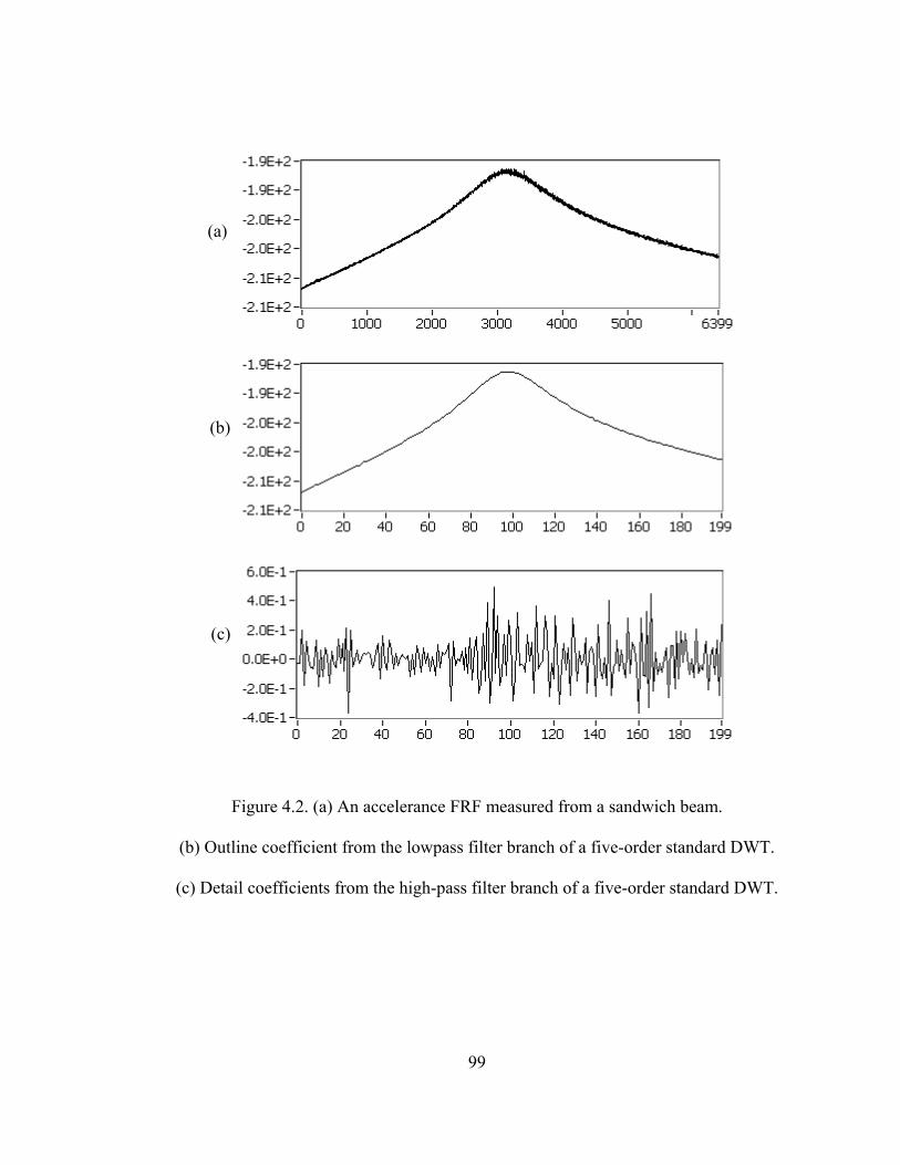
99
Figure 4.2. (a) An accelerance FRF measured from a sandwich beam.
(b) Outline coefficient from the lowpass filter branch of a five-order standard DWT.
(c) Detail coefficients from the high-pass filter branch of a five-order standard DWT.
(a)
(b)
(c)

100
Figure 4.3. (a) A simulated noisy accelerance FRF with natural frequency of 200 Hz and
damping ratio of 2%. (b) Denoising result from a five-order undecimated wavelet
transform with the calculated natural frequency of 199.79 Hz and damping ratio 1.99%.
(a)
(b)

101
Figure 4.4. (a) A free vibration signal measured from an aluminum cantilever beam. (b) The wavelet scalogram.
(c) The original Gabor coefficients. (d) The Gabor spectrogram.
101
(a) (b)
(c) (d)

102
Figure 4.5. (a) The original Gabor coefficients of signal shown in Fig 4.4 (a).
(b) (c) (d) The modified Gabor coefficients of three modes by using three mask matrices.
(a)
(b)
(c)
(d)

103
Figure 4.6. The decoupled modal responses using Gabor expansion.
(a) The first mode, (b) the second mode, (c) the third mode, and
(d) spectra of the three reconstructed signals.
(a)
(b)
(c)
(d)
104
Figure 4.7. Damping calculation simulation using the Gabor transform.
(a) A simulated free vibration signal, (b) the original Gabor coefficients of this signal,
(c) and (d) the reconstructed modal responses, and
(e) and (f) envelopes established using the Hilbert transform and the best exponential fits.
(a) (b)
(c) (d)
(e) (f)

105
Figure 4.8. Damping calculation simulation using the Gabor spectrogram.
(a) A simulated free vibration signal, (b) the Gabor spectrogram,
(c) and (d) the two vibration modes calculated using zoom Gabor spectrogram.
(b)
(a) (c)
(d)

106
Figure 4.9. The original complex FFT of a free vibration signal containing three modes.
(a) Real part, (b) imaginary part.

107
Figure 4.10. Comparison of the envelopes of the displacement components
reconstructed using the FFT and Gabor expansion methods.
(a) First mode, (b) second mode, (c) third mode.

108
Figure 4.11. Experimental setup for modal testing.
108

109
Figure 4.12. Comparison of the theoretical and measured mode shapes.
109

110
CHAPTER 5 ANALYSIS OF SOUND TRANSMISSION THTROUGH
SANDWICH PANELS
Sound transmission loss (TL), or referred to as the sound reduction index, of a panel
is the difference between the incident sound power level and the transmitted sound power
level for a specified frequency or frequency band. This number indicates the noise
insulation capability of the panel. The sound transmission loss is often an important
consideration in the analysis and design of partitions or panels separating adjoining
spaces in industry, housing and various types of vehicles. It can be described in terms of
the panel impedance Z [127]. For a homogeneous thin panel, if the stiffness and the
damping are neglected at low frequencies, the panel impedance depends purely on its
surface density. In this case, i sZ ωρ= , where ρs is the mass per unit area of the panel. In
such a simple case, the sound transmission loss is determined by “mass law” which says
that the TL increases by 6 dB per octave [128]. However, for a real panel, the TL depends
not only on the surface density, but on its bending stiffness, damping loss factor and the
orientation of the incident sound waves as well. Due to the coincidence effect, when the
free flexural wave speed of the panel Cp, which increases with frequency, approaches the
speed of sound in air, the impedance of the panel to incident sound wave ceases to be
mass-like and the TL becomes much less than that given by mass law. The frequency at
which the coincidence effect begins to occur is called the critical coincidence frequency

111
(often known as simply as the critical frequency). For an isotropic homogeneous panel,
the critical frequency is given by
2
2cl
cfcπκ
= , (5-1)
where c is the sound wave speed in air, κ is the radius of gyration of the panel, and cl is
the speed of longitudinal wave propagating in the panel. Note that / 12tκ = for a
rectangular cross-section panel with thickness t, and /lc E ρ= for a homogeneous
material. An intuitive solution is to raise the critical frequency of the panel out of the
audio frequency range. However, from Eq. (5-1) we can see this means either reducing
the thickness of the panel or reducing the stiffness to density ratio. Unfortunately, in
practice, most of the panels must also serve as structural partitions. From an engineering
point of view, a reduction in the stiffness to density ratio may degrade the performance of
the whole structure in other respects. So improving the sound transmission loss without
compromising the stiffness to density ratio is an interesting problem.
This chapter will start with a brief literature review of the sound transmission of
sandwich structures. A theoretical prediction of the TL of a three-layer sandwich
structure is performed using statistical energy analysis (SEA). Some optimization
considerations are presented as well. Experimental results are discussed at the end of the
chapter.
5.1 Review of the Sound Transmission Loss of Sandwich Panels
Research on the sound transmission loss of sandwich structures can be traced back
to 1959. Kurtze and Watters undertook a very early design study of sandwich plates and

112
analyzed their acoustical behavior [129]. By inserting a soft core between two thin face
sheets, the shear waves, which are not dispersion waves, are introduced in a wide middle
frequency range. If the shear wave speed is less than the speed of sound in air, the critical
frequency is then shifted to higher frequencies, which avoids locating the critical
frequency in the range of interest. They derived the impedance of a sandwich plate and
the speed of transverse wave propagation through the structure using a circuit analogy.
They also designed a periodic wall structure in which bridges are used to connect the
face-sheets of the composite. Their experimental results agree with the theoretical
estimation of the anti-symmetric motion. However, since they assumed that the core
material is incompressible, their model cannot predict the symmetric thickness motion
which was studied subsequently by other researchers.
Ford, Lord and Walker assumed instead the polyurethane foam core as
compressible material, and they studied both the anti-symmetric (or flexural) and
symmetric (or dilatational) modes of vibration [130]. However, as pointed out later by
Smolenski and Krokosky, the energy expression used in [130] is incorrect. Smolenski and
Krokosky corrected the energy expression and investigated the influence of the core
material properties on the critical frequency due to the dilatation mode [131]. They also
measured the TL of two panels with different configurations and explained the
discrepancies between the predicted and experimental results.
Dym, Lang and their colleagues conducted a series of researches on the sound
transmission of sandwich plates [132-136]. Dym and Lang derived five equations of
motion for sandwich panels with identical face sheets in [133]. The five equations are
decoupled into two sets which represent the symmetric and anti-symmetric vibration

113
modes. They also calculated the impedance for both the symmetric and anti-symmetric
cases, thus obtaining the TL as well. Note that an error in [132] was corrected later in
[134]. Lang and Dym presented optimal TL properties for sandwich panels using indirect
and direct methods [133]. They reported that an increase in the stiffness of the core would
eliminate the coincidence effect caused by the symmetric vibration mode. However, the
anti-symmetric coincidence effect would still occur at a low frequency. Dym and Lang
later expanded their theoretical model to include infinite sandwich panels with unequal
isotropic face sheets and an elastic orthotropic core [135]. They assumed the presence of
damping in both the face sheets and the core.
Ordubadi and Lyon studied the effect of orthotropy on the sound transmission
through plywood panels [137]. By assuming that the bending stiffness and phase wave
speed change gradually from the stiff direction to the soft direction of the orthotropic
panels, they presented an analytical expression for the TL of such panels.
Narayanan and Shanbhag used Mead’s [41] equations of motion of viscoelastically
damped sandwich panels to study the sound transmission characteristics [139]. Their
parametric study shows that the transmission loss is more sensitive to the variation of the
core shear parameter than to the change of other parameters. However, since Mead’s
model only considered flexural vibration modes, Narayanan and Shanbhag’s analysis did
not include the dilatational modes. They only calculated the TL at some particular angles
of incidence rather than integrating the results to obtain the field incident representation.
Moore and Lyon developed analytical models for sandwich panels with isotropic
and orthotropic cores [140]. They considered both the flexural and dilatational modes.
This analysis describes the propagation of shear and dilatational waves within the

114
sandwich panel cores and their interaction with face-sheets in the transmission of sound
through the panels. For dilatational modes, coincidence occurs near the conventional
double wall resonance frequency, which is determined by the stiffness of the core and the
mass of the face sheets. They further developed a design approach which lowers the
double wall resonance frequency to below the frequency band of interest, and shifts the
critical frequency to higher frequencies.
Wang, Sokolinsky, Rajaram and Nutt derived expressions to predict the TL in
infinitely wide sandwich panels using two models, (1) the consistent high-order
approach, and (2) the two-parameter foundation model [141]. In both the models, the TL
is calculated using a decoupled equation which represent the symmetric and anti-
symmetric motions. They compared their numerical prediction with experimental results.
The consistent high-order approach is more accurate, while the two-parameter foundation
model is more convenient.
The TL of multi-layer panels has also been analyzed by some other researchers.
Guyander and Lesueur studied the equation of motion, the modal density and the TL of
viscoelastic and orthotropic multi-layer plates [142-144]. They used both plane wave and
reverberation sound excitations to study the TL. Panneton and Atalla developed a three-
dimensional finite element model to predict the TL through a multi-layer system made of
elastic, acoustic and porous-elastic media [145]. The three-dimensional Biot theory was
used to model the porous-elastic medium. However, at low frequencies (lower than 100
Hz, and sometimes even 200 Hz), the predicted behavior is completely incorrect. For
higher frequencies, the model is only useful for unbonded plates. Kurra and Arditi used
the ASTM and ISO standards to measure the sound transmission loss of multi-layered

115
plates [146,147]. Uris and Estelles studied the sound transmission of multi-layered
sandwich plates using different configurations of polyurethane and polystyrene layers
[148]. They found that multi-layered sandwich plates possess better sound transmission
loss, and the coincidence effect is not as obvious as with three-layer sandwich plates.
These observations are actually because multi-layered plates are much thicker and the
surface densities help to increase the sound transmission loss.
5.2 Prediction of Sound Transmission through Sandwich Panels using SEA
As discussed in Chapter 2, SEA method was first developed by Lyon and others in
the 1960’s. Crocker and Price used SEA to predict the sound transmission loss of
isotropic single-layered panels [15]. The same theoretical model is used for the sandwich
panels.
The subsystems and energy flow relationship are illustrated schematically in Fig.
5.1. The subscripts represent the subsystem number. The source room and the receiving
room are the first and third subsystems, and the panel under study is the second
subsystem. Here the two rooms are assumed to be reverberant. This means that the sound
pressure level measured in each room is the same at any position in that particular. 1inW is
the power input from loudspeakers in the source room, diW is the power dissipated in the
i-th subsystem, and ijW is the power flow from the i-th to the j-th subsystem.

116
Figure 5.1. Schematic of the power flow in three-coupled systems using SEA.
If only the source room is excited using loudspeakers and there is no other power
input to the other subsystems, the power balance equations can be expressed as:
1 1 12 13
12 2 23
3 13 23
,,.
in d
d
d
W W W WW W WW W W
⎫= + +⎪= + ⎬⎪= + ⎭
(5-2)
The power dissipated in a system in a specified frequency band is related to the
energy stored in the system, iE , through the internal loss factor iη , namely,
di i iW Eωη= , (5-3)
where ω is the center frequency of the frequency band. The power flow between
subsystems i and j is
( ),jiij ij i
i j
EEW nn n
ωη= − (5-4)
loudspeaker input power
inW1
dW1
12W 23W
13W
dW2dW3
1E 2E 3E

117
where ni and nj are the modal densities of subsystems i and j, and ηij is the coupling loss
factor from subsystem i to subsystem j. The equation i
j
ji
ij
nn
=ηη
must be satisfied.
Applying Eq.s (5-4) to (5-2) gives the power balance of the partition in a frequency
band with the center frequency ω:
1 212 21 2 2 2 2 23
1 2
( )E EW n E En n
ωη ωη ωη= − = + . (5-5)
Note that generally 3 3 1 1/ /E n E n<< , so the 3 3/E n term is neglected in Eq. (5-5). Here the
coupling loss factors η23 and η23 are related to the sound radiation efficiency σrad:
22 rad
21 23 rads
c ππ ρ ση η η
ρ ω= = = . (5-6)
The subscript 2π means that 2radπσ represents the one-sided radiation efficiency. Since the
source room sound field is assumed to be reverberant, the energy stored in it is expressed
by the pressure p1, and volume V1:
21
211 / cVpE ρ>=< . (5-7)
The mechanical energy stored in the panel is expressed by its velocity and mass:
ps AvE ρ>=< 22 , (5-8)
where ρs and Ap are the surface density and area of the panel.
Combining the results above, the averaged squared velocity of the panel is obtained
2 22 rad2 1 1
2 21 rad 22 s p
n V pvn A c
π
π
ηη η ρ ρ
< >< >= ⋅ ⋅ ⋅
+. (5-9)
Thus the power radiated by the resonant modes into the receiving room is
2 223 radpW cA vπρ σ= < > . (5-10)

118
Similarly, 13 13 1W Eωη= . The coupling loss factor η13 due to non-resonant random
incidence mass-law transmission is obtained from [15]
10 13 RI 101
10 log TL 10log4
pA cV
ηω
⎛ ⎞= − + ⎜ ⎟
⎝ ⎠, (5-11)
2 2RI 10 10TL 10log 10log ln(1 )a a⎡ ⎤= − +⎣ ⎦ , (5-12)
where / 2sa cωρ ρ= , and TLRI is called the random incidence transmission loss.
Substituting (5-12) in (5-11), η13 can be derived as
2 3 2 2
13 3 2 2 21
ln 14
p s
s
A cV c
ρ ω ρηω ρ ρ
⎡ ⎤= +⎢ ⎥
⎣ ⎦. (5-13)
2 2 21
13 2 2 2ln 1( ) 4
p s
s
p A cW
cρ ω ρ
ωρ ρ⎡ ⎤
⇒ = +⎢ ⎥⎣ ⎦
. (5-14)
In the source room, the sound power incident on the dividing partition of area pA is:
21
inc 4 ppW A
cρ< >
= . (5-15)
Below the critical frequency, the sound transmission loss of a finite panel is more
controlled by the contribution of those modes that have their resonance frequencies
outside the frequency band of the excitation signal than by those with resonance
frequencies within that band. So taking into account both the forced and resonant penal
motions, the transmission coefficient can be approximated by
inc2 2 2
223 13 rad2 1rad2 2 2 2
1 rad 2
/ 41
ln 12 ( ) 4
p
p s
s s
A cWA cW W n V
n c c
ππ
π
ρρτ η ω ρσ
η η ρ ωρ ρ
= =+ ⎡ ⎤
⋅ ⋅ ⋅ + +⎢ ⎥+ ⎣ ⎦
. (5-16)
Then, the sound transmission loss TL can be calculated by

119
TL 10log(1/ )τ= . (5-17)
For a given panel and enclosure, Ap, ρs, V1, n1, and ρc are constants. So, in order to
optimize the sound transmission loss, we narrow the problem down to some properties of
the sandwich panel: the modal density n2, the internal loss factor η2, and the radiation
efficiency 2radπσ .
5.2.1 Modal density
The modal density is defined as the number of vibration modes of a system in a unit
frequency interval. It can be derived from the wavenumber space as shown in Fig. 5.2.
For a given frequency ω, the wavenumber of an isotropic plate, 2 2x yk k k= + , forms a
quarter of a circle. If all the boundaries are simply-supported, for a plate with side lengths
a and b, the modal count N(ω) and modal density n(ω) are
2
24( )4
pk A
N k
a b
π
ω π π π= =
⋅,
2( )( )4
pAdN dknd dωωω π ω
⇒ = = ⋅ . (5-18)
Most of the researchers simplified the equation of motions of a sandwich panel to fourth-
order, although they deal with sandwich beams using sixth-order equations [59,100,105].
However, as shown in Chapter 3, the equation of motion of sandwich panels should be
sixth-order. In this chapter the equation derived by Mead is used [41]:
6 4 2 6 2 2( ) (1 ) 0f f s sD w g D Y w w g wρ ω ρ ω ν∇ − + ∇ − ∇ + − = . (5-19)

120
Here w is the transverse displacement of the sandwich panel, Df is the bending stiffness
of one face sheet about its own neutral axis, as defined in Chapter 3, ρs is the surface
density of the sandwich panel, and ν is the Poisson ratio of the panel. For symmetric
sandwich panels, the two parameters are 2 / 2f fY d E t= , and 2 / f f cg G E t t= . By
assuming simple harmonic solution, the wavenumber k can be obtained by the use of the
bi-cubic equation:
2 226 4 2 2
21 3 (1 ) 0s s
f f f
gdk g k kt D D
ρ ω ρ ω ν⎛ ⎞
+ + − − − =⎜ ⎟⎜ ⎟⎝ ⎠
. (5-20)
Then the modal density can be calculated using Eq. (5-18) by solving for k2 from Eq. (5-
20). Note that although Eq. (5-18) is derived from simply-supported panels, the shape and
the boundary conditions do not affect the result much. However, as shown in Fig. 5.2 (b),
if the panel is not isotropic, the wavenumber k does not form a quarter of a circle. In this
case, the value of k solved using Eq. (5-20) is angle dependent, because both Ef and G
change with angle. Then modal count must then be modified as
/ 22
20
( ) ( , )2
pAN k d
π
ω ω φ φπ
= ∫ . (5-21)
5.2.2 Analysis of critical frequency
As discussed before, the critical frequency is the frequency at which the speed of
flexural waves in the panel is the same as the speed of sound wave in air. By setting
2 / pk f Cπ= , and 343 m/spC = , and substituting these in Eq. (5-20), the critical
frequency of a sandwich panel can be found as
21 42 2cf B B C
π= + + , (5-22)

121
where
4 22
2
(343) 1 3 (343)s
f f
dB gD t
ρ ⎛ ⎞= − +⎜ ⎟⎜ ⎟
⎝ ⎠, (5-23)
62(343) (1 )s
f
gCD
ρ ν= − . (5-24)
Next we will simplify the expressions for B and C to study the relationship between
the critical frequency and other parameters. If the core is thick enough compared to the
face sheet, then we have c f cd t t t= + ≈ . Substituting this and the expression of parameter
g into Eq.s (5-23) and (5-24), then,
2 2 24
3 3
4 2
3 3
2 ( 3 ) (343)12 (343)
12 (343) 6 (343) ,
fs
f f f f c
s
f f f f
G t dB
E t E t t
GE t E t
ρ
ρ
⋅ + ⋅×= −
× ×≈ −
(5-25)
62
2 4
24 (343) (1 )s
f f c
GCE t t
ρ ν× ⋅ ⋅= −
⋅ ⋅. (5-26)
Since the surface density ρs increases with an increase in the core thickness, it can
be seen, from Eqs. (5-25) and (5-26), that both B and C increase, if other parameters do
not change. Consequently, the critical frequency increases with an increase in the core
thickness. However, this conclusion is only valid in some range, because it is drawn from
Eq. (5-20) which is derived for a thin panel. Intuitively, the critical frequency should
decrease with an increase in the thickness.
Other cases are relatively more complicated. For example, a change in the face
sheet thickness leads to changes in the surface density and shear modulus of the entire
panel. The Young’s and shear moduli, however, generally change simultaneously, but not

122
necessarily in the same direction. So for different sandwich panels, it is not easy to
predict the trend of the change in the critical frequency. In most the cases, the critical
frequency needs to be evaluated quantitatively based on the material properties and
geometry of the sandwich panel under study. However, one can use Eq. (5-22) as a guide
to select appropriate materials so that the critical frequency can be removed from the
frequency range in which human hearing is most sensitive.
5.3 Experimental Results and Discussion
5.3.1 Transmission loss measurement using two-room method
As described in the previous section, the two-room method was used to determined
the sound transmission loss in the Sound and Vibration Laboratory at Auburn University.
The two-room suite consists of two reverberation rooms. The panels under investigation
were mounted in the window in the walls between the two rooms, as shown in Fig. 5.3.
The volumes of the source room and receiving room are 51.15 m3 and 51.51 m3,
respectively. The area of the panels under test is 0.36 m2. In order to reduce
environmental noise, each room has two walls made of wood with fiberglass filled in
between them. The two rooms are also separated from each other using fiberglass, and
mounted on air bags to reduce the flanking transmission between them. The inner walls
of both rooms are made with materials with low absorption coefficients so that the rooms
have long reverberation times and the sound fields therein can be assumed to be diffuse.
However, since each sound field is not completely diffuse, the sound absorption in each
should be taken into account. By assuming that the panel under test is the only path that

123
the sound travels through, the sound transmission loss measured using the two-room
method is given by
2 21 2
2 2
TL 10log NR 10log24 ln10 24 ln10
p R p Rp p
A cT A cTL L
V V= − + = + , (5-27)
where Lp1 and Lp2 are the sound pressure levels measured in the two rooms, and TR1 and
V2 are the reverberation time and volume of the receiving room [149].
Table 5.1 lists the properties of the panels in study. Two homogenous aluminum
panels were pre-tested in order to make sure the measurement procedure was correct
because the sound transmission properties of aluminum panels are already known.
First of all, the reverberation times in the receiving room were measured for each
panel using B&K PULSE system. Table 5.2 shows the reverberation times measured for
one-third octave frequency bands from 80 Hz to 8 kHz.
Then a steady white noise is generated using two loudspeakers and an air jet nozzle
in the source room. The air jet nozzle was used to increase the noise level in the high
frequency region. The sound pressure levels in two rooms were measured using two
B&K microphones, type 4188, whose optimized frequency response range is from 8 Hz
to 12.5 kHz. For each panel listed in Table 5.1, the measurements of the sound pressure
levels in both the source and receiving rooms (Lp1 and Lp2) were repeated eight times by
putting the two microphones at eight randomly selected positions. The spatial averages
were calculated to obtain the noise reduction (NR). Note that the background noise in the
receiving room was also measured and subtracted from Lp2. The sound transmission loss
was then calculated using Eq. (5-20).

124
5.3.2 Transmission loss measurement using sound intensity method
The sound intensity measurement technique using the cross-spectrum of two
microphones was presented by Fahy, and Waser and Crocker [150,151]. This technique
was then used in the sound transmission loss measurement by Crocker and other
researchers [151,152]. The experimental setup is shown in Fig. 5.3 (b). In this technique,
the receiving room is changed from a reverberation room to an anechoic room. The
anechoic room can be constructed using wedges or fiberglass rolls with very high sound
absorption capability so that the sound field can be assumed to be essentially a free field.
An intensity probe is used to measure the sound intensity in the anechoic room, LI2. Then
the sound transmission loss is the difference in the sound intensity levels incident the on
the panel and transmitted by it into anechoic room:
2
1 2 2TL4
iI I I
pL L L
cρ= − = − , (5.28)
where 2ip is the spatial average of the incident sound pressure square.
Compared to the two-room method, the sound intensity method is less time
consuming, and it is not necessary to measure the reverberation times in the receiving
room. However, a disadvantage of the sound intensity method is the frequency limitations.
The low frequency limit is due to the phase mismatch between the two microphones. The
high frequency limit is caused by the finite distance approximation error [151]. The
intensity probe used in the Sound and Vibration Laboratory is a B&K type 3548, which
has two ½ inch microphones, and its optimal frequency range is from 125 Hz to 5 kHz
when a 12 mm spacer is used.

125
Figure 5.4 compares the sound transmission loss of Panel A using the two-room
method and the sound intensity method. The two results are in good agreement. The
maximum difference is about 2 dB. Because the sound field in the anechoic room is not
an ideal free field, the measured sound intensity level, LI2, also contains some reflected
sound. This makes the measured transmitted sound intensity level somewhat less than the
true value, especially for frequency bands higher than the critical frequency.
So considering the frequency range limit of the sound intensity method, the
conventional two-room method was used to measure the sound transmission loss.
5.3.3 Radiation efficiency
As discussed before, the radiation efficiency of a panel is an important parameter
needed in the prediction of its sound transmission loss using SEA. The radiation
efficiency can be obtained experimentally by measuring the radiation resistance Rrad. The
radiation resistance is defined as the ratio of the sound power radiated to the space
averaged mean-square value of the panel’s normal velocity: 2rad rad s,t
/R W v= . With the
two-room method measurement setup, the panel was excited by a shaker using write
noise. One microphone was located in each room to measure the sound radiated from the
panel under the external excitation. An accelerometer was used to measure the panel
response. For each panel, the sound pressure levels in the two rooms and the acceleration
responses were measured at eight randomly selected positions, and averages were made.
The two-sided radiation resistance of the panel is given by
24 3 31 1rad 2
1 3
13.8 ,a R R
S VS VRS c T T
π ωρ
⎡ ⎤= +⎢ ⎥
⎣ ⎦ (5-29)
126
where S1, S3, Sa are the power spectral density functions of the signals obtained from the
two microphones and the accelerometer, V1 and V3 are the volumes of the source room
and the receiving room, respectively, and TR1 and TR3 are the reverberation times of the
two rooms [15]. The radiation efficiency is then expressed as
42 radrad 2 p
RA c
ππσ
ρ= . (5-30)
5.3.4 Simulation using AutoSEA
AutoSEA is an interactive vibro-acoustics simulation tool based on the SEA
method. In order to calculate the sound transmission loss and the radiation efficiency of a
panel, two virtual rooms and a panel must be created in AutoSEA, as shown in Fig. 5.5.
The two virtual rooms were assumed each to have a diffuse sound field, and to have the
identical volumes as do the two real rooms in the Sound and Vibration Laboratory. A
random sound source was used to simulate the white noise generation in the source room.
The panel under investigation has clamped boundary conditions. For an isotropic
aluminum panel, the material and geometric properties, such as mass density, Young’s
modulus, Poisson’s ratio, thickness, area and perimeter must be defined. To create a
sandwich panel in AutoSEA, the material properties of the face sheets and the core are
required separately. The face sheets of a sandwich panel must only be isotropic while the
core can be orthotropic. The material properties assumed for the face sheets and the core
are listed in Appendix B.
The internal loss factor in AutoSEA can be frequency dependent. The loss factors
for all of the one-third octave bands, which are called the damping spectra, were

127
predefined and input to the software based on the measured damping loss factors. Note
that the sound transmission loss depends on the internal damping, while the radiation
efficiency does not.
5.3.5 Experimental and simulation results
In order to verify the experimental method, measurements on two aluminum panels
were carried out first, because the radiation and sound transmission properties of
isotropic materials have been well established. Figures 5.6 and 5.7 compare the measured
radiation efficiency and sound transmission loss of Panel E, with the results simulated
using AutoSEA software in which the internal loss factor was set to 1%. It can be seen
that the measured results agree quite well with the results simulated using AutoSEA.
Both the measured and the simulated results show the critical frequency at 4000 Hz
which is the same as the one calculated using Eq. (5-1). Below the critical frequency, the
radiation efficiency increases with frequency. At the critical frequency, it reaches a
maximum value. Above the critical frequency, the radiation efficiency decreases to a
plateau level. The discrepancies between the measured and the simulated results in the
low frequency region are mainly because the area of the panel is not large enough. Since
the modal density of a homogenous aluminum panel is constant, there are not enough
modes at low frequencies to make a good statistical frequency average of the sound
transmission loss.
Figures 5.8 and 5.9 show the measured and simulated radiation efficiency of Panels
A and B. The predictions using AutoSEA are quite close to the measured results.
However, it should be noted that for frequencies higher than the critical frequency, the

128
radiation efficiency does not decrease to a plateau value. Sandwich and isotropic panels
thus appear to have a different behavior.
Figures 5.10 and 5.11 illustrate the measured and simulated sound transmission loss
of Panels A and B. For Panel A, two cases with different values of damping were
evaluated with AutoSEA. The first damping spectrum used the measured loss factors as
shown in Chapter 3. In this case, the internal loss factor increases with frequency. In the
other case, the loss factor was assumed to be constant, 2%, in all the frequency bands. By
comparing the two simulated cases with the measured result, it can be seen that the
simulated result with measured frequency-dependent damping is closer to the measured
result. This means that for the sound transmission loss prediction using SEA, the
frequency-dependent damping is more suitable.
The first natural frequency of Panel A mounted in the window is about 170 Hz. At
frequencies below the first natural frequency, the behavior of the panel is stiffness
controlled. This explains the dip in the sound transmission loss curve in the 160 Hz band
in Fig.11. Since the face sheets in Panel B are twice thick as those in Panel A, the first
natural frequency is higher. It can be seen in Fig.12 that the dip in the sound transmission
loss is in the 200 Hz band.
The measured sound transmission loss results of all the panels used in the study are
shown in Fig. 5.13. In order to quantify and compare the overall sound transmission loss
properties of these panels, their sound transmission classes (STC) were calculated using
the procedure defined in ASTM standard E413-87. These sound transmission class values
are listed in the legend of Fig. 5.13. It is seen that the sound transmission loss values of
all the four sandwich panels are smaller than those of the two aluminum panels. This

129
implies that the surface mass density still dominates the overall transmission loss
behaviors of these panels. The foam-filled honeycomb sandwich design does not
demonstrate any advantage of sound transmission over heavier metal counterpart,
although the sandwich structures have higher damping. That means such a foam-filled
honeycomb sandwich design must be modified if it is to obtain higher sound transmission
loss.
For further comparison, another aluminum panel with a similar surface mass
density to the studied sandwich panels was simulated in AutoSEA. The thickness of this
aluminum panel was set to 1 mm. Its surface density is 2.7 kg/m3 which is very close to
the surface density values of Panels A, B and C. Figure 5.14 compares the calculated TL
of such an aluminum panel with the measured TL of Panel A. Since the simulated
aluminum panel is thinner than Panels E and F, its critical frequency increases to 12.5
kHz. The STC values also show that the overall TL of the aluminum panel is higher than
the sandwich panels studied.

130
Panel Core thickness (mm)
Face sheet thickness (mm)
Density (kg/m3)
Surface density (kg/m2)
A 6.35 0.33 327.75 2.41
B 6.35 0.66 336.97 2.57
C 12.7 0.66 190.96 2.50
D 25.4 0.66 130.25 3.28
E 3.175 mm thick homogeneous aluminum 8.57
F 6.35 mm thick homogeneous aluminum 17.15
Table 5.1. Geometry parameters of panels under study.

131
Center frequency (Hz) Panel A Panel B Panel C Panel D Panel E Panel F
80 0.380 0.375 0.421 0.377 0.370 0.370 100 0.632 0.544 0.557 0.506 0.574 0.675 125 0.493 0.395 0.352 0.360 0.405 0.374 160 0.636 0.659 0.699 0.634 0.634 0.610 200 0.578 0.740 0.736 0.698 0.740 0.643 250 0.903 0.818 0.856 0.860 0.865 0.887 315 1.048 1.086 1.034 1.043 1.079 1.110 400 1.240 1.162 1.155 1.111 1.196 1.190 500 1.264 1.254 1.309 1.345 1.293 1.329 630 1.316 1.407 1.324 1.344 1.362 1.349 800 1.411 1.449 1.473 1.430 1.420 1.376 1000 1.326 1.364 1.368 1.338 1.309 1.335 1250 1.238 1.248 1.224 1.247 1.203 1.235 1600 1.132 1.157 1.121 1.146 1.144 1.136 2000 1.028 1.036 1.016 1.016 1.033 0.983 2500 0.947 0.916 0.947 0.937 0.912 0.960 3150 0.846 0.809 0.865 0.830 0.846 0.861 4000 0.778 0.759 0.780 0.747 0.764 0.782 5000 0.698 0.688 0.690 0.713 0.702 0.709 6300 0.633 0.639 0.629 0.652 0.629 0.632 8000 0.556 0.545 0.555 0.538 0.526 0.541
Table 5.2. Reverberation times of the receiving room with different panels.
131

132
kx
ky
kx
ky
k
k
π/a
π/b
(a)
(b)
Figure 5.2. Modal distribution of (a) isotropic and (b) anisotropic plates.

133
(a)
(b)
Figure 5.3. Side views of (a) the two reverberation rooms, and (b) experimental setup for
transmission loss measurements using sound intensity method.
Panel
Air Bags
Source Room Receiving Room
Fiberglass

134
0
5
10
15
20
25
0 500 1000 1500 2000 2500 3000 3500
Frequency (Hz)
Tran
smis
sion
Los
s (d
B)
intensity probe methodtwo-room method
Figure 5.4. Comparison of sound transmission loss measurements of composite Panel A
using two-room method and sound intensity method.
134

135
Figure 5.5. Sound transmission loss model using AutoSEA software.
Source room Receiving room
Plate under investigation
Sound source
135

136
-35
-30
-25
-20
-15
-10
-5
0
5
10
80 125 200 315 500 800 1250 2000 3150 5000 8000
Frequency (Hz)
Rad
iatio
n ef
ficie
ncy
(dB
)
measured resultAutoSEA result
Figure 5.6. The measured and simulated radiation efficiency of Panel E.
Rad
iatio
n ef
ficie
ncy
10lo
g(σ)
136

137
0
5
10
15
20
25
30
35
40
45
50
100 1000 10000
Frequency (Hz)
Tran
smis
son
Loss
(dB
)
measured result
AutoSEA with loss factor 1%
mass law
Figure 5.7. Sound transmission loss of Panel E.
fc = 4000 Hz
137

138
-20
-15
-10
-5
0
5
10
15
80 125 200 315 500 800 1250 2000 3150 5000 8000Frequency (Hz)
Rad
iatio
n ef
ficie
ncy
(dB
) measured resultAutoSEA result
Figure 5.8. Measured and simulated radiation efficiency of Panel A.
Rad
iatio
n ef
ficie
ncy
10lo
g(σ)
138

139
-20
-15
-10
-5
0
5
10
15
80 125 200 315 500 800 1250 2000 3150 5000 8000
Frequency (Hz)
Rad
iatio
n ef
ficie
ncy
(dB
) measured resultAutoSEA result
Figure 5.9. Measured and simulated radiation efficiency of Panel B.
Rad
iatio
n ef
ficie
ncy
10lo
g(σ)
139

140
0
5
10
15
20
25
30
80 125 200 315 500 800 1250 2000 3150 5000 8000Frequency (Hz)
Tran
smis
sion
loss
(dB
)
measured result
AutoSEA (with measured damping values)
AutoSEA (2% constant loss factor)
Figure 5.10. The measured and simulated sound transmission loss of Panel A.
140

141
0
5
10
15
20
25
30
80 125 200 315 500 800 1250 2000 3150 5000 8000
Frequency (Hz)
Tran
smis
sion
loss
(dB
)
measured resultAutoSEA result
Figure 5.11. Measured and simulated transmission loss of Panel B.
141

142
.
Figure 5.12. Comparison of sound transmission loss and sound transmission class of panels studied.
0
5
10
15
20
25
30
35
40
45
50
125 200 315 500 800 1250 2000 3150 5000
Frequency (Hz)
Tran
smis
sion
Los
s (d
B)
Panel A (STC = 14 dB)Panel B (STC = 15 dB)Panel C (STC = 15 dB)Panel D (STC = 17 dB)Panel E (STC = 25 dB)Panel F (STC = 26 dB)
142

143
0
5
10
15
20
25
30
35
40
80 160 315 630 1250 2500 5000 10000 20000
Frequency (Hz)
Tran
smis
sion
loss
(dB
)measured Panel A (STC = 14 dB)
1mm aluminum (STC = 20 dB)
Figure 5.13. Comparison of sound transmission loss and sound transmission class of Panel A
with an aluminum panel having the same surface density.
143

144
CHAPTER 6 ANALYSIS OF FOAM-FILLED HONEYCOMB
CORES USING FEM
As we study the dynamics of foam-filled honeycomb sandwich structures, an
important issue associated with the material properties is the honeycomb cell size effect.
Onck et al. analyzed the size effect of pure hexagonal honeycombs on the Young’s and
shear moduli in terms of the ratio α, of the honeycomb width, b, to the cell size, D, as
shown in Fig. 6.1 [153,154]. They reported that as the integer value of α increases, or the
honeycomb cell size decreases relative to the specimen size, the Young’s modulus
increases to a plateau level which is called the bulk Young’s modulus of the honeycomb.
This is due to the increased constraint of the cell walls at the free surface and the
decreasing area fraction of the open-cell walls. However, for non-integer values of α, the
Young’s modulus drops as α increases from one integer to the next. As shown in Fig. 6.1,
the longitudinal cell walls of a honeycomb carry most of the uniaxial load. As α varies
from one integer to the next, the number of longitudinal cell walls in the width direction
does not change, but the cross-sectional area increases. This results in the Young’s
modulus drop when α varies from one integer to the next. Figure 6.2 shows the change in
the Young’s modulus with respect to α [153].
As discussed in the previous chapters, the sandwich structures with foam-filled
honeycomb cores show some advantages compared with pure honeycomb cores. By
filling foam in the honeycomb cells, not only the longitudinal cell walls but also the foam

145
can carry the uniaxial load. So the foam is expected to reduce the discontinuity of the
Young’s modulus observed with pure honeycomb cores.
Onck et al. only derived the theoretical expressions for the honeycomb beam of one
cell wide, α = 1, which is the simplest case [153]. Compared to the use of the finite
element method, the theoretical derivation for honeycomb beams with higher values of α
will be much more difficult. So Onck et al. used the finite element software ABAQUS to
study those more complicated cases.
Similar finite element models were developed to analyze the material properties of
foam-filled honeycombs using ANSYS, and are presented in this chapter. Sections 6.1
and 6.2 describe the modeling procedure and present results of the effect of cell size on
the Young’s modulus and shear modulus. Composite materials may have a negative value
of Poisson’s ratio. The influence of Poisson’s ratio is studied in Section 6.3. The
relationship between the cell size and other properties is discussed as well.
6.1 Size Effect on the Young’s Modulus
Gibson and Ashby stated that the Young’s moduli of a honeycomb in the L- and W-
directions are the same if the cell size is sufficiently small [155]. That means that there
are a large number of honeycomb cells in both the L- and W-directions. In this case the
bulk Young’s modulus Ebulk in both the L- and W-directions of a honeycomb is
3
bulk4
3wE tE
l⎛ ⎞= ⎜ ⎟⎝ ⎠
, (6-1)
where Ew is the Young’s modulus of the honeycomb cell wall, and t and l are the
thickness and length of the cell wall as shown in Fig. 6.3. Figure 6.3 illustrates a section
of a honeycomb and the beam model of the cell wall. D is the cell size which is the

146
distance from two parallel cell walls, 3D l= , and d is the thickness of the whole
honeycomb.
If there is only one cell in the W-direction, or α = 1, then the compression modulus
in the L-direction becomes
3* 2
3wE tE
l⎛ ⎞= ⎜ ⎟⎝ ⎠
, (6-2)
which is one half of the result calculated using Eq. (6-1).
A finite element model was developed using ANSYS to study the Young’s modulus
of the foam-filled honeycombs. The basic idea is to build a beam as shown in Fig 6.1 and
calculate the deflection δ under a uniaxial pressure P. Then the Young’s modulus can be
obtained. All the foam-filled honeycombs have the same width, b = 30 mm, and thickness,
0.25 inch 6.35 mmd = = . As the cell size is varied, the number of cells in the width
direction varies accordingly. The bottom end of the beam is assumed clamped. Since the
foam is much softer than the honeycomb wall, a single force applied on the top of the
beam may cause stress concentration. Instead, the uniaxial load is simulated by imposing
a uniform pressure of 10,000 Pa on the top.
Since the model is assumed to be a plane stress problem, the whole beam is
simplified using a 2-D model. The honeycomb cell walls are modeled using beam
elements (BEAM3), as shown in Fig. 6.3 (b). The cross-sectional area, area moment of
inertia and cell wall thickness are input as “Real Constants” to the database. The foam in
honeycomb cells is modeled using triangular elements (PLANE2) with the same
thickness as the whole foam-filled honeycomb beam. Note that the cell wall thickness, t,
and the foam-filled honeycomb beam thickness, d, are different.

147
The honeycomb walls are assumed to be isotropic with the Young’s modulus
109.5 GPawE = , Poisson’s ratio 0.35wν = , and density 533 kg/m3. These values are
provided by honeycomb manufacturer, Hexcel Corporation. According to these values,
the bulk Young’s modulus of a pure honeycomb structure is bulk 120 MPaE = .
Polyurethane foam is assumed to be orthotropic in the x-y plane, but isotropic in the
thickness direction. Polyurethane foams are categorized into several quality grades. The
material properties used in Chapter 6 are those of Grade 120 Polyurethane foam tested in
[155]. They are foam 22 MPaE = , and foam 13.3 MPaG = . Poisson’s ratio is set to be 0.4.
Before running the foam-filled honeycomb finite element models, a pre-test was
conducted for a pure honeycomb beam with α = 1. The calculated compression modulus
is 61 MPa, which is the same as the result calculated using Eq. (6-2). This result verifies
that the finite element model is feasible.
The calculated Young’s moduli of foam-filled honeycomb beams with different cell
sizes are listed in Table 6.1. Note that for different cell sizes, the cell thickness-to-length
ratio is set to be constant, t/l = 0.078, which is the same ratio used in [153]. The cell wall
constants and volume ratios are also listed in Table 6.1. From reference [155], for
hexagonal honeycombs, the ratio of the volume of honeycomb walls to the volume of the
entire structure is
honeycomb
total
23
V tV l
= . (6-3)
When t/l = 0.078, Vhoneycomb/Vtotal = 9%.
From Table 6.1 some conclusions can be drawn: (1) The most significant effect of
the honeycomb cell size is that the Young’s modulus increases as the cell size decreases

148
(α increases). This is because the honeycomb cells become denser as structural elements
so that the constraint increases at the boundary. This trend is the same as that predicted in
reference [153]. However, unlike the non-integer α cases, because of foam filled in
honeycombs, there are no non-load-carrying honeycomb cell walls when α is non-integer.
So as α varies from one integer to the next, the Young’s modulus still increases instead.
(2) The Young’s modulus of foam-filled honeycombs is greater than those of the
corresponding pure honeycombs and pure foam, and even greater than the simple
summation of the Young’s moduli of the pure honeycomb and foam. (3) As the cell size
is decreased, the volume percentage of honeycomb also decreases to the theoretical value
of 9% calculated using Eq. (6-3). Considering that polyurethane foam is less costly than
honeycombs, these conclusions indicate that even though the volume of the honeycomb
cells decreases, the cell size decrement will lead to cheaper and stiffer structures.
6.2 Size Effect on the Shear Modulus
Gibson and Ashby give the bulk shear modulus of pure honeycombs with a
sufficiently large number of cells in the width direction as follows [155]
3
bulk 3wE tG
l⎛ ⎞= ⎜ ⎟⎝ ⎠
. (6-4)
For the honeycomb materials investigated in this chapter, bulk 30 MPaG = . After foam is
filled in the honeycomb cells, the constraints at the boundary become larger compared
with the pure honeycomb structures. So the bulk shear modulus of a foam-filled
honeycomb structure is higher than the value calculated using Eq. (6-4). However, the
relationship between the honeycomb cell size and the shear modulus is not obvious.

149
Smaller cell size leads to dense honeycomb frame, which seems to increases the
constraints at the boundaries. On the other hand, since the thickness of the honeycomb
cell wall also decreases when the cell size becomes smaller, it is hard to predict
analytically how the constraints at the boundary actually change with the cell size. So a
finite element model was developed in ANSYS to study the effect of cell size on the
shear modulus of the foam-filled honeycomb structures.
In order to simulate pure shear deformation, the translation in the y-direction of
both the upper and lower edges is restricted, as shown in Fig. 6.4 (a), so that these two
edges can only slide in the x-direction. The shear forces are simulated using a series of
forces of the same magnitude applied along the two edges with uniform distribution. The
shear deformation angle should be measured on the centerline. For all samples with
different cell size simulated in ANSYS, the total shear force is the same, 8 N. This means
although the force distribution along the boundary becomes denser when the cell size is
increased, the magnitude of each distributed force element is decreased, so that the
summation of the shear force is always equal to 8 N.
Note that in order to obtain accurate results, one dimension, for example the x-
direction in Fig. 6.4 (a) of the specimen, must be longer than the other dimension. The
aspect ratio should be around 4. This value is obtained from some trail-and-error
calculations for aluminum samples modeled using triangular elements and isotropic
material properties with the Young’s modulus (70 GPa) and Poisson’s ratio (0.3). The
theoretical shear modulus value is then 26.9 GPa. Table 6.2 lists the calculated shear
moduli for different aspect ratios using the finite element model, and relative error
compared with the theoretical value of 26.9 GPa.

150
The same beam and triangle elements used in the previous section were used to
model the honeycomb cell walls and foam in ANSYS to study the cell effect on the shear
modulus. Figure 6.4 (b) illustrates the deformed element mesh under pure shear forces.
Table 6.3 lists the calculated shear moduli of foam-filled honeycombs with different cell
sizes. It can be concluded that after foam is filled in the honeycomb cells, the shear
modulus of the structure becomes larger than that of a pure honeycomb calculated using
Eq. (6-4). As the cell size is decreased, the shear modulus also decreases, which is
opposite to the change in the Young’s modulus. This means as the cell size is decreased,
although the honeycomb frame becomes denser, the cell walls become thinner, which
decrease the constraints at the boundary, and therefore decreases the shear modulus of the
whole foam-filled honeycomb structure.
Figure 6.5 presents a plot of the results listed in Tables 6.1 and 6.3 in terms of α. It
can be seen that as the cell size is decreased, both the Young’s modulus and the shear
modulus converge to plateau values which are the bulk Young’s modulus and shear
modulus.
6.3 Influence of Poisson’s Ratio
Poisson’s ratio values of conventional materials are generally positive with a
theoretical upper limit of 0.5 [157]. However, the development of composite materials
has made negative Poisson’s ratio values possible. Although hexagonal honeycombs
always have positive Poisson’s ratios, honeycombs of different shapes and foams can
possess negative Poisson’s ratios. Figure 6.6 shows three foam microstructures which
have negative values of Poisson’s ratio from [155]. Figure 6.6 (a) shows an inverted

151
shape, which can be produced from conventional foams in a variety of ways. Figure 6.6
(b) shows solid cylinders or spheres attached to each other by thin elastic strips or wires.
When the structure is stretched in the direction of the arrows, the ligaments unwrap from
the cylinders or spheres, causing them to rotate. Therefore the structure expands in other
directions. The structure shown in Fig 6.6(c) is an example of a family of open tensile
networks of nodes, linked by simple tensile springs, and constrained by hinged
inextensible rods or threads. When the material is stretched axially, such constraints force
a lateral expansion.
For simplification, the foam modeled in this section is assumed to be isotropic.
Since ( )2 1
EGν
=+
, a negative Poisson’s ratio will increase the shear modulus if the
Young’s modulus does not change. In addition, under longitudinal compression, the foam
elements with negative Poisson’s ratio do not expand, but also become compressed, in
the transverse direction. This phenomenon also increases the compression modulus in the
longitudinal direction.
Figures 6.7 and 6.8 show the influence of Poisson’s ratio on the Young’s modulus
and the shear modulus of foam-filled honeycombs. Both the Young’s modulus and the
shear modulus decrease as the Poisson’s ratio increases from -0.8 to 0.4. From the
discussion in the previous two sections, we know that the size effects are not significant,
when the cell size is small enough relative to the sample size, because both the Young’s
modulus and the shear modulus converge to the bulk values. However, Figs. 6.7 and 6.8
imply that the material properties can be dramatically modified by changing the Poisson’s
ratio of the foam. For example, the Young’s modulus of the foam-filled honeycomb with

152
cell size of 4 mm increases from 149.65 MPa to 346.85 MPa (2.3 times stiffer) with a
change of Poisson’s ratio from 0.4 to -0.8.
6.4 More Considerations of Cell Size Effects
So far we have seen that the material properties of foam-filled honeycombs can be
changed considerably by varying the honeycomb cell size and the Poisson’s ratio of the
polyurethane foam. These effects are quite useful in the design stage. One can obtain the
optimal design according to meet the application goal. However, it should be stated that
these effects may be contrary to those needed for different functions of sandwich
structures. For example, we always expect high stiffness since the sandwich elements
work as structural parts in most engineering applications. On the other hand, as discussed
in Chapter 5, sandwich structures are expected to be soft in shear so that the shear wave
speed is less than the speed of sound in air. Merely decreasing the honeycomb cell size
satisfies both the requirements. Smaller cell sizes also lead to lighter structures.
However, foam with negative Poisson’s ratio will increase both the Young’s
modulus and the shear modulus. An increased Young’s modulus will also increase the
critical frequency. If the critical frequency is in the high frequency range, one may be
able to increase the critical frequency out of the frequency band of interest by increasing
the Young’s modulus. Unfortunately, as shown in Fig. 5.6, the critical frequency of
asandwich plate is usually in low frequency range. So an increase of stiffness will shift
the critical frequency towards the frequency band of interest.
Therefore, a trade-off between the overall stiffness and the sound transmission
properties should be considered in the design stage.

153
Cell size (mm)
α Cell wall
length (mm)
Cell wall thickness (mm)
Cross-sectional area (m2)
Moment of inertia (m4)
Young’s modulus
(MPa)
Volume ratio Vhoneycomb/Vtotal (%)
30 1 17.32 1.35 8.57e-6 1.30e-12 93.20 10.99
20 1.5 11.55 0.90 5.72e-6 3.86e-13 113.09 10.10
15 2 8.66 0.68 4.32e-6 1.66e-13 124.69 9.91
12 2.5 6.93 0.54 3.43e-6 8.33e-14 130.56 9.65
10 3 5.77 0.45 2.86e-6 4.82e-14 136.48 9.55
7.5 4 4.33 0.34 2.15e-6 2.04e-14 140.58 9.42
6 5 3.46 0.27 1.72e-6 1.04e-14 144.78 9.33
5 6 2.89 0.23 1.43e-6 6.03e-15 146.15 9.29
4 7.5 2.31 0.18 1.14e-7 3.09e-15 149.03 9.23
Table 6.1. Cell size effect on the Young’s modulus of foam-filled honeycomb beams.
153

154
Aspect ratio Calculated shear modulus (GPa) Relative error (%)
1 17.9 -33.50
2 23.76 -11.75
3 25.3 -5.95
4 26.6 -1.11
5 25.4 -5.58
6 25.5 -5.20
Table 6.2. Influence of aspect ratio on the shear modulus calculation using FEM.

155
Cell size (mm) Length (m) Aspect ratio Shear deformation (m) Shear modulus (MPa)
30 0.13856 4.62 0.29113e-5 93.7
15 0.12124 4.83 0.92062e-5 52.9
10 0.11547 3.85 1.54958e-5 47.2
7.5 0.11258 3.75 1.07763e-5 45.3
6 0.110828 3.69 1.38337e-5 44.2
5 0.12701 4.23 1.67838e-5 43.8
3 0.117776 3.93 1.43748e-5 42.6
Table 6.3. Cell size effect on the shear modulus of foam-filled honeycomb beams.
155

156
Figure 6.1. (a) A section of the honeycomb structure. (b) Beam element used to model
the honeycomb cell wall.
x (W)
δ
y (L)
pb = αD

157
Figure 6.2. Cell size effect on the Young’s modulus of pure honeycomb structures.

158
t
d
l(b)
d
l (a)
Dx
yz
Figure 6.3. (a) A section of the honeycomb structure.
(b) Beam element used to model the honeycomb cell wall.

159
Figure 6.4. (a) Schematic of the shear modulus calculation.
(b) Foam-filled honeycomb finite element mesh and pure shear deformation.
x
yγ
F
F b = αD
(a)
(b)
159

160
60
70
80
90
100
110
120
130
140
150
160
1 2 3 4 5 6 7 8 9 10
number of honeycomb cells, α
Youn
g's
mod
ulus
(MPa
)
30
40
50
60
70
80
90
100
Shea
r mod
ulus
(MPa
)
Young's modulusshear modulus
Figure 6.5. Honeycomb cell size effect on Young’s modulus and shear modulus of foam-filled honeycomb structures.
160

161
Figure 6.6. Microstructures giving negative Poisson’s ratios [155]. (a) Inverted “reentrant” cell shape.
(b) Solid cylinders or spheres attached to each other by elastic strips.
(c) Nodes, connected by tensile springs, and constrained by hinged inextensible rods.
(a) (b) (c)
161

162
0
50
100
150
200
250
300
350
400
-0.8 -0.7 -0.6 -0.5 -0.4 -0.3 -0.2 -0.1 0 0.1 0.2 0.3 0.4
Poisson ratio
Youn
g's
mod
ulus
of f
oam
-fille
d ho
neyc
omb
(MPa
)
cell size 4 mmcell size 5mmcell size 6mmcell size 7.5 mmcell size 10 mmcell size 15 mmcell size 30 mm
Figure 6.7. Influence of Poisson’s ratio on the Young’s modulus of foam-filled honeycomb structures.
cell size increases
162

163
0
20
40
60
80
100
120
140
-0.8 -0.7 -0.6 -0.5 -0.4 -0.3 -0.2 -0.1 0 0.1 0.2 0.3 0.4
Poisson Ratio
shea
r mod
ulus
of f
oam
-fille
d ho
neyc
omb
(MPa
)
cell size 3 mmcell size 5 mmcell size 6 mmcell size 7.5 mmcell size 10 mmcell size 15 mmcell size 30 mm
Figure 6.8. Influence of Poisson’s ratio on the shear modulus of foam-filled honeycomb structures.
cell size increases
163

164
CHAPTER 7 CONCLUSIONS
The research objects in this dissertation are sandwich beams and plates with the
core made of paper honeycomb filled with polyurethane foam. The honeycomb material
is expected to increase the stiffness of the entire structure, and the foam improves the
damping. In this research, the static strain-stress relationship was studied, and the
equations of motion were derived using Hamilton’s principle. The expressions of the
wavenumber and speed of flexural wave in sandwich beams and plates were obtained.
Based on both statics and dynamics studies, the frequency dependence of damping was
analyzed for foam-filled honeycomb sandwich beams, in which the face sheets are much
thinner than the core, or the structural parameter is large. It was found that if the face
sheet thickness is increased, the damping in the low and high frequency ranges is
decreased, but it remains high in the middle frequency range. If the thickness of the core
is increased, the damping is increased in the middle and high frequency ranges.
Delamination introduces more friction in a composite beam structure and thus makes the
damping increase. However, delamination also reduces the stiffness as well as the natural
frequencies of sandwich structures. Experiments on beams with different configurations
and with delamination were carried out. The experimental results are consistent with the
analytical predictions.
A wavelet analysis-based noise reduction technique was used for damping
calculations using frequency response function analysis. Unlike the traditional digital

165
wavelet transform, the undecimated wavelet transform is time-invariant, and does not
depend on the denoising-threshold selection which may lead to quite different results if
the traditional digital wavelet transform is used. The results obtained from simulated
signals show quite high accuracy.
A new damping calculation method was developed using the Gabor transform and
Gabor spectrogram. This method was developed for free vibration signals. Since the
amplitude of free vibration signal decreases exponentially, the signal is not stationary.
Both linear and quadratic Gabor analyses can decompose the signal onto the joint time-
frequency domain, and have a globally optimal time-frequency resolution compared to
the wavelet analysis. By using the Gabor transform and expansion (linear Gabor
analysis), the time signal can be reconstructed after a noise reduction process in the time-
frequency domain. The complex analytic signal of the reconstructed time signal is then
constructed using the Hilbert transform. Then the damping ratio can be calculated based
on the best exponential fit of the analytic signal’s envelope. The Gabor spectrogram
method cannot be used to reconstruct the time signal, but it can be used to calculate the
damping ratio using ridge detection techniques.
The linear Gabor transform and expansion procedure can also be applied to modal
testing without force information. For an N-DOF system, in general a vibration signal
contains the dynamic deflection of N modes if these modes are all properly excited. The
Gabor transform and expansion can be used to decouple and reconstruct these modes to
effectively make them into single-mode signals. Then the natural frequency, modal
damping, vibration magnitude and phase can be extracted for each mode. The mode
shape can also be obtained by comparing the magnitudes and phase angles at different

166
grid points. Compared to the FFT-based decoupling/reconstruction, the Gabor expansion
method benefits from higher SNR. The measurements were made on a cantilever beam.
Without any information on the excitation, the modal parameters can be obtained very
well using the Gabor expansion approach.
The analysis of the sound transmission loss of foam-filled honeycomb sandwich
panels was carried out. A theoretical model was developed using the statistical energy
analysis (SEA) method. For a given sandwich panel, the sound transmission loss depends
on its internal damping, modal density and radiation efficiency. The internal damping can
be estimated using the method presented in Chapter 3. The modal density can be obtained
by calculating the wavenumber using a bi-cubic function. A parameter study was made
for the sound transmission loss. It can be concluded that an increase in the core thickness
will increase the critical frequency. Two measurement methods, the two-room method,
and the sound intensity method, were compared. The sound intensity method is less
complicated than the two-room method, but restricted in an optimal frequency band
which is narrower than that in the two-room method. Measurements on six different
panels, including two isotropic aluminum panels and four sandwich panels, were carried
out using the two-room method. Simulations of the radiation efficiency and sound
transmission loss were conducted using AutoSEA software. The measured results agree
with quite well with the results simulated using AutoSEA. It was found that the radiation
efficiency of the foam-filled honeycomb sandwich panels does not decrease at
frequencies beyond the critical frequency. The surface densities of the sandwich panels
are much smaller than those of the aluminum panels. The measured results show that the
overall sound transmission loss values of sandwich panels are smaller than those of the

167
aluminum panels. This implies that the surface density still dominates the overall
transmission loss behavior of these panels. The foam-filled honeycomb sandwich design
does not show any sound reduction advantage over their heavier metal counterparts,
although the sandwich structures have higher damping capacity. That means such a foam-
filled honeycomb sandwich design must be modified to obtain higher sound transmission
loss properties. The measured transmission loss curves also show that the critical
frequency increases as the core thickness is increased, if other parameters do not change,
which agrees with the theoretical prediction.
The honeycomb cell size effects on the Young’s modulus and the shear modulus of
the foam-filled honeycomb structures were studied using finite element models
developed in ANSYS. As the cell size is decreased, the honeycomb cells become denser,
and the honeycomb frame is more resistant to external loads, although the volume ratio is
smaller. This effect increases the Young’s modulus. Reference [153] studied the cell size
effect of pure honeycomb structures, and reported the same trend for integer values of α,
the number of cells in the width direction, while for non-integer values of α, the Young’s
modulus was found to decrease as α is increased from one integer to the next. However,
for foam-filled honeycomb structures, the Young’s modulus does not decrease as non-
integer values of α increase from one integer to the next. For pure honeycomb structures,
only longitudinal cell walls carry the external loads. When non-integer values of α are
increased from one integer to the next, the number of longitudinal cell walls in the width
direction does not increase, but the cross-section area increases. On the contrary, for the
foam-filled honeycomb structures, the longitudinal honeycomb cell walls, as well as the
foam, carry the external loads. Even when non-integer value of α is increased, the foam

168
in those open cells still can carry external loads. The shear modulus, on the other hand,
decreases as the cell size is decreased. This is because the cell walls become thinner,
which decreases the constraints at the boundary.
Hexagonal honeycomb structures always have positive Poisson’s ratio. However,
polyurethane foam can possess a negative value of Poisson’s ratio. By filling honeycomb
cores with foam having a negative value of Poisson’s ratio, both the Young’s modulus
and the shear modulus increase dramatically. It is worth noticing that the effects of cell
size and Poisson’s ratio may have opposite effects and can be used to achieve different
functional purposes with sandwich structures. A trade-off between the overall stiffness
and the sound transmission properties may be made in the design stage.
This research work has approved that the foam-filled honeycomb sandwich design
does not show any advantage of sound reduction advantaged over their heavier metal
counterparts, although the sandwich structures have higher damping capacity. So an
important future work is to improve the sound transmission properties of sandwich
structures using different design or different material elements, such as braided material
and nano-material.

169
REFERENCES
[1] D. Zenkert, An Introduction to Sandwich Construction. EMAS publishing, London (1997)
[2] D. Zenkert, The Handbook of Sandwich Construction. EMAS publishing, London (1997)
[3] J. M. Davies, Lightweight Sandwich Construction. Blackwell Science, Condon (2001)
[4] W. J Jung, A. J. Aref, “A Combined Honeycomb and Solid Viscoelastic Material for Structural Damping Application”, Mechanics and Materials. 53(8), 831-844 (2003)
[5] J. E. Ruzicka, Structural Damping. ASME, New Jersey (1959)
[6] B. J. Lazan, Damping of Materials and Members in Structural Mechanics. Pergamon Press, London (1968)
[7] A. D. Nashif, D. I. G. Jones, J. P. Henderson, Vibration Damping. John Wiley & Sons, Inc., New York (1985)
[8] D. I. G. Jones, Handbook of Viscoelastic Vibration Damping. John Wiley & Sons, Inc., New York (2001)
[9] C. T Sun, Y. P. Lu, Vibration Damping of Structural Elements. Prentice Hall PTR, Englewood Cliffs, NJ (1995)
[10] C. F. Beards, Structural Vibration Analysis: Modeling, Analysis, and Damping of Vibrating Structures. Halsted Press, Chichester (1983)
[11] E. E. Ungar, “Structural Damping”, Chapter 12 in Noise and Vibration Control Engineering: Principles and Applications, Leo. L. Beranek (Editor). John Wiley & Sons, Inc. (1992)
[12] D. J. Mead, Passive Vibration Control. John Wiley & Sons, New York (1999)
[13] R. H. Lyon, G. Maidanik, “Power Flow between Linearly Coupled Oscillators”, Journal of the Acoustical Society of America. 34(5), 623-639 (1962)
[14] G. Maidanik, “Response of Ribbed Panels to Reverberant Acoustic Fields”, Journal of the Acoustical Society of America. 34(6), 809-826 (1962)
[15] M. J. Crocker, A. J. Price, “Sound Transmission using Statistical Energy Analysis”, Journal of Sound and Vibration. 9(3), 469-486 (1969)
[16] B. L. Clarkson, K. T. Brown, “Acoustic Radiation Damping”, ASME Journal of Vibration, Acoustics, Stress and Reliability in Design. 107, 357-360 (1985)

170
[17] D. J. Mead, “Plates with Regular Stiffening in Acoustic Media; Vibration and Radiation”, Journal of the Acoustical Society of America. 88(1), 391-401 (1990)
[18] S. Gade & H. Herlufsen, Damping measurement. Bruel and Kjaer Technical Review (1994)
[19] M. J. Crocker, Encyclopedia of Acoustics Vol II. John Wiley & Sons, Inc., New York (1997)
[20] D. J. Ewins, Modal Testing: Theory, Practice and Application. Research Studies Press LTD, Baldock, England (2000)
[21] M. D. Rao, “Recent applications of viscoelastic damping for noise control in automobiles and commercial airplanes”, Journal of Sound and Vibration. 262(3) 457–474 (2003)
[22] B. C. Nakra, “Vibration Control with Viscoelastic Materials”, Shock and Vibration Digest. 8(6), 3-12 (1976)
[23] B. C. Nakra, “Vibration Control with Viscoelastic Materials - II”, Shock and Vibration Digest. 13(1), 17-20 (1981)
[24] B. C. Nakra, “Vibration Control with Viscoelastic Materials - III”, Shock and Vibration Digest. 16(5), 17-22 (1984)
[25] P. J. Torvik, “The Analysis and Design of Constrained Layer Damping Treatments”, Damping Applications for Vibration Control. AMD-Vol 38, ASME, Chicago, IL (1980)
[26] R. Chandra, S. P. Singh, K. Gupta, “Damping Studies in Fiber-Reinforced Composites - A Review”, Composite Structures. 46, 41-51 (1999)
[27] H. G. Alalen, Analysis and Design of Structural Sandwich Panels. Pergamon Press, London (1969)
[28] E. M. Kerwin, “Damping of Flexural Waves by a Constrained Viscelastic Layer”, Journal of the Acoustical Society of America. 31(7), 952-962 (1959)
[29] D. Ross, E. E. Ungar, E. M. Kerwin, “Damping of plate flexural vibrations by means of viscoelastic laminate”, Structural Damping. 49-88, ASME, New Jersey (1959)
[30] E. E. Ungar, “Loss Factors of Viscoelasticlly Damped beam Structures”, Journal of the Acoustical Society of America. 34(8), 1082-1089 (1962)
[31] E. E. Ungar and E. M. Kerwin, “Loss Factors of Viscoelastic System in Terms of Energy Concepts”, Journal of the Acoustical Society of America. 34(7), 954-957 (1962)
[32] J. E. Ruzicha, “ Damping Structural Resonances using Viscoelastic-Damping Mechanisms, Part I Design Configurations”, ASME Journal of Engineering for Industry. 83, 403-413 (1961)
[33] J. E. Ruzicha, “ Damping Structural Resonances using Viscoelastic-Damping Mechanisms, Part II Experimental Results”, ASME Journal of Engineering for Industry. 83, 414-424 (1961)

171
[34] Y. Y. Yu, “Damping of Flexural Vibrations of Sandwich Plates”, Journal of the Aerospace Sciences. 29, 790-803 (1962)
[35] Y.V.K. Sadasivia Rao, B.C.Nakra, “Vibrations of Unsymmetrical Sandwich Beams and Plates with Viscoelastic Cores”, Journal of Sound and Vibration. 34(3), 309-326 (1974)
[36] R. A. DiTaranto, “Theory of Vibratory Bending for Elastic and Viscoelastic Layered Finite-Length Beams”, ASME Journal of Applied Mechanics. 32, 881-886 (1965)
[37] R. A. DiTaranto, W. Blasingame, “Effect of End Constraints on the Damping of Laminated Beams”, Journal of the Acoustical Society of America. 39(2), 405-407 (1966)
[38] R. A. DiTaranto, W. Blasingame, “Composite Damping of Vibrating Sandwich Beams”, ASME Journal of Engineering for Industry. 89, 633-638 (1967)
[39] D. J. Mead, S. Markus, “The Forced Vibration of a Three-Layer, Damped Sandwich Beam with Arbitrary Boundary Conditions”, Journal of Sound and Vibrations. 10(2), 163-175 (1969)
[40] D. J. Mead, S. Markus, “Loss Factors and Resonant Frequencies of Encastré Damped Sandwich Beam”, Journal of Sound and Vibrations. 12(1), 99-112 (1970)
[41] D. J. Mead, “The Damping Properties of Elastically Supported Sandwich Plates”, Journal of Sound and Vibrations, 24(3), 275-295 (1972)
[42] D. J. Mead, “Governing Equations for Vibrating Constrained-Layer Damping Sandwich Plates and Beams”, ASME Journal of Applied Mechanics. 40, 639-640 (1973)
[43] D. J. Mead, “Loss Factors and Resonant Frequencies of Periodic Damped Sandwich Plates”, ASME Journal of Engineering for Industry. 98, 75-80 (1976)
[44] D. J. Mead, “A Comparison of Some Equations for the Flexural Vibration of Damped Sandwich Beams”, Journal of Sound and Vibrations. 83(3), 363-377 (1982)
[45] M. J. Yan, E. H. Dowell, “Governing Equations for Vibrating Constrained-Layer Damping Sandwich Plates and Beams”, ASME Journal of Applied Mechanics. 39, 1041-1046 (1972)
[46]M. J. Yan, E. H. Dowell, “Elastic Sandwich Beam or Plate Equations Equivalent to Classical Theory”, ASME Journal of Applied Mechanics. 41, 526-527 (1974)
[47] P. Cupial and J. Niziol, “Vibration and Damping Analysis of a Three-Layered Composite Plate with a Viscoelastic Mid-Layer”, Journal of Sound and Vibrations. 183(1), 99-114 (1995)
[48] Horng-Jou Wang, Lien-Wen Chen, “Vibration and damping analysis of a three-layered composite annular plate with a viscoelastic mid-layer”, Composite Structures. 58, 563-570 (2002)
[49] S. He, M. D. Rao, “Vibration and Damping Analysis of Multi-Span Sandwich Beams with Arbitrary Boundary Conditions”, Journal of Sound and Vibration. 164(1) 125-142 (1993)

172
[50] D. K. Rao, “Vibration of Short Sandwich Beams”, Journal of Sound and Vibration. 52(2), 253-263 (1977)
[51] D. K. Rao, “Frequency and Loss Factors of Sandwich Beams under Various Boundary Conditions”, Journal of Mechanical Engineering Science. 20(5), 271-282 (1978)
[52] S. J. Hwang, R. F. Gibson, “The Use of Strain energy-Based Finite Element Techniques in the Analysis of Various Aspects of Damping of Composite Material and Structures”, J. Composite Materials. 26(17), 2585-2605 (1992)
[53] S. J. Hwang, R. F. Gibson, “The effects of Three-Dimensional States of Stress on Damping of Laminated Composites”, Composites Science and Technology. 41, 379-393 (1991)
[54] S. J. Hwang, R. F. Gibson, J. Singh, “Decomposition of Coupling effects on Damping of Laminated Composites under Flexural Vibration”, Composites Science and Technology. 43, 159-169 (1992)
[55] R. F. Gibson, Principles of Composite Mechanics. McGraw-Hill, New York (1994)
[56] S. J. Hwang, R. F. Gibson, “Contribution of Interlaminar Stresses to Damping in Thick Laminated Composites under Uniaxial Extension”, Composite Structures. 20, 29-35 (1992)
[57] B. J. Lazan, “Energy Dissipation Mechanisms in Structures, with Particular Reference to Material Damping”, Structural Damping. 1-34, ASME, New Jersey (1959)
[58] A. C. Nilsson, “Wave propagation in and sound transmission through sandwich plates”, Journal of Sound and Vibration. 138(1), 73-94 (1990)
[59] E. Nilsson, A. C. Nilsson, “Prediction and measurement of some dynamic properties of sandwich structures with honeycomb and foam cores”, Journal of Sound and Vibration. 251(3), 409-430 (2002)
[60] A. W. van Vuure, I. Verpoest, F. K. Ko, “Sandwich-Fabric Panels as Spacers in a Constrained Layer Structural Damping Application”, Composites Part B: Engineering. 32, 11-19 (2001)
[61] J. A. Agbasiere, P. Groothenhuis, “Flexural Vibration of Symmetrical Multi-Layer Beams with Viscoelastic Damping”, Journal of Engineering Science. 10(3), 269-281 (1968)
[62] P. Groothenhuis, “The Control of Vibrations with Viscoelastic Materials”, Journal of Sound and Vibration. 11(4), 421-433 (1970)
[63] B. C. Nakra, P. Groothenhuis, “Structural Damping Using a Four-Layer Sandwich”, ASME Journal of Engineering for Industry. 94, 81-86 (1972)
[64] N. T. Asnani, B. C. Nakra, “Vibration Damping Characteristics of Multilayered Beams with Constrained Viscoelastic Layers”, ASME Journal of Engineering for Industry. 98, 895-901 (1976)
173
[65] N. Alam, N. T. Asnani, “Vibration and Damping Analysis of Multilayered Rectangular Plates with Constrained Viscoelastic Layers”, Journal of Sound and Vibration. 97(4), 597-614 (1984)
[66] N. Alam, N. T. Asnani, “Vibration and Damping Analysis of Fibre einforced Composite Material Plates”, Journal of Composite Materials. 20, 2-18 (1986)
[67] N. Alam, N. T. Asnani, “Refined Vibration and Damping Analysis of Multilayered Rectangular Plates”, Journal of Sound and Vibration. 119(2), 347-362 (1987)
[68] A. Bhmaradi, “Sandwich Beam Theory and the Analysis of Constrained Layer Damping”, Journal of Sound and Vibration. 179(4), 591-602 (1995)
[69] M. D. Rao, S. He, “Dynamic Analysis and Design of Laminated Composite Beams with Multiple Damping Layers”, AIAA Journal. 31(4), 736-745 (1993)
[70] S. He, M. D. Rao, “Longitudinal Vibration and Damping Analysis of Adhesively Bonded Double Strap Joints”, ASME Journal of Vibration and Acoustics. 114, 330-337 (1992)
[71] B. K. Nanda, A. K. Behera, “Damping in Layered and Jointed Structure”, International Journal of Acoustics and Vibration. 5(2), 89-95 (2000)
[72] E. R. Marsh, L. C. Hale, “Damping of Flexural Waves with Imbedded Viscoelastic Materials”, ASME Journal of Vibration and Acoustics. 120, 188-193 (1998)
[73] S. Prasad, L. A. Carlsson, “Debonding and Crack Kinking in Foam Core Sandwich Beams – I. Analysis of Fracture Specimens”, Engineering Fracture Mechanics. 47(6), 813-824 (1994)
[74] S. Prasad, L. A. Carlsson, “Debonding and Crack Kinking in Foam Core Sandwich Beams – II. Experimental Investigation”, Engineering Fracture Mechanics. 47(6), 825-841 (1994)
[75] H. Luo, S. Hanagud, “Dynamics of Delaminated Beams”, International journal of Solid and Structures. 37(10), 1501-1519 (2000)
[76] H.Y. Kim, W. Hwang, “Effect of Debonding on Natural Frequencies and Frequency response Functions of Honeycomb Sandwich Beams”, Composite Structures. 55, 51-62 (2002)
[77] Y. Frostig, “Behavior of delaminated sandwich beam with transversely flexible core –– high order theory”, Composite Structures. 20(1), 1-16 (1992)
[78] D. J. Mead, “Criteria for Comparing the Effectiveness of Damping Treatments” Noise Control. 7, 27-38 (1961)
[79] Y. P. Lu, B. E. Douglas, “On the Forced Vibrations of Three-Layer Damped Sandwich Beams”, Journal of Sound and Vibration. 32(4), 513-516 (1974)
[80] Y. P. Lu, J. W. Killian, G. C. Everstine, “Vibrations of Three Layered Damped Sandwich Plate Composites”, Journal of Sound and Vibration. 64(1), 63-71 (1979)
[81] Y. P. Lu, G. C. Everstine, “More One Finite Element Modeling of Damped Composite Systems”, Journal of Sound and Vibration. 69(2), 199-205 (1980)

174
[82] J. W. Killian, Y. P. Lu, “A Finite Element Modeling Approximation for Damping Material Used in Constrained Damped Structures”, Journal of Sound and Vibration. 97(2), 352-354 (1984)
[83] Y. P. Lu, J. C. Clemens, A. J. Roscoe, “Vibrations of Composite Plate Structures Consisting of a Constrained-Layer Damping Sandwich with Viscoelastic Core”, Journal of Sound and Vibration. 153(3), 552-558 (1992)
[84] C. D. Johnson, D. A. Kienholz, “Finite element prediction of damping in structures with constrained viscoelastic layers”, AIAA Journal. 20(9), 1284-1290 (1981)
[85] D. E. Veley, S. S. Rao, “Two-dimensional finite element modeling of constrained layer damping”, Smart structures and Materials 1994: Passive Damping, C. D. Johnson (Editor), Proc. SPIE 2193. 276-283 (1994)
[86] A. Zambrano, J. A. Inaudi, J. M. Kelly, “Accuracy of the Modal Strain Energy Method”, Smart structures and Materials 1994: Passive Damping, C. D. Johnson (Editor), Proc. SPIE 2193. 284-295 (1994)
[87] T. S. Plagianakos, D. A. Saravanos, “High-Order Layerwise Mechanics and Finite Element for the Damped Dynamic Characteristics of Sandwich Composite Beams”, International journal of Solid and Structures. 41(24-25), 6853-6871 (2004)
[88] P. J. Shorter, “Wave propagation and damping in linear viscoelastic laminates”, Journal of the Acoustical Society of America. 115(5), 1917-1925 (2004)
[89] D. J. McTavish, P. C. Hughes, Finite element modeling of linear viscoelastic structures: the GHM method. Proceedings of 33rd AIAA/ASME/ASCE/AHS/AHS Structures, Structural Dynamics and Materials Conference, Paper No. AIAA-92-2380-CP. (1992)
[90] G. Wang, S. Veeramani, N. M. Wereley, Analysis of sandwich plates with isotropic face plates and a viscoelastic core. ASME Journal of Vibration and Acoustics. 122, 305-312 (2000)
[91] X. Chen, H. L. Chen, X. L. Hu, “Damping Prediction of Sandwich Structures by Order-Reduction-Iteration Approach”, Journal of Sound and Vibration. 222(5), 803-812 (1999)
[92] S. A. Nayfeh, “Damping of flexural vibration in the plane of lamination of elastic–viscoelastic sandwich beams”, Journal of Sound and Vibration. 276(3-5), 689-711 (2004)
[93] R. H. Lyon, R. G. DeJong, Theory and Applications of Statistical Energy Analysis. RH Lyon Corp, Massachusetts (1998)
[94] B. Bloss, M. D. Rao, “Measurements of Damping in Structures by the Power Input Method”, Experimental Techniques. 26(3), 30-33 (2002)
[95] J.P.D. Wilkinson, “Modal Densities of Certain Shallow Structural Elements”, Journal of the Acoustical Society of America. 43(2), 245-251 (1968)
[96] L.L Erickson, “Modal Densities of Sandwich Panels: Theory and Experiment”, The Shock and Vibration Bulletin. 39(3), 1-16 (1969)

175
[97] B. L. Clarkson, R J Pope, “Experimental determination of modal densities and loss factors of flat plates and cylinders”, Journal of Sound and Vibration. 77(4), 535-549 (1981)
[98] B. L. Clarkson, “The derivation of modal densities from point impedances”, Journal of Sound and Vibration. 77(4), 583-584, (1981)
[99] M. F. Ranky, B. L. Clarkson, “Frequency averaged loss factors of plates and shells”, Journal of Sound and Vibration. 89(3), 309-323 (1983)
[100] B. L. Clarkson, M. F. Ranky, “Modal density of honeycomb plates”, Journal of Sound and Vibration. 91(1), 103-118 (1983)
[101] K. T. Brown, “Measurement of modal density: an improved technique for use on lightly damped structures”, Journal of Sound and Vibration. 96(1), 127-132 (1984)
[102] K. T. Brown, M. P. Norton,” Some comments on the experimental determination of modal densities and loss factors for statistical energy analysis applications”, Journal of Sound and Vibration. 102(4), 588-594 (1985)
[103] P.R. Keswick, M. P. Norton, “A Comparison of Modal Density Measurement Techniques”, Applied Acoustics. 20 (2), 137-153 (1987)
[104] B. Hakansson, P. Carlsson, “Bias Errors in Mechanical Impedance Data Obtained with Impedance Head”, Journal of Sound and Vibration. 113(1), 173-183 (1987)
[105] K. Renji, P. S. Nair and S. Narayanan, “Modal density of composite honeycomb sandwich panels” Journal of Sound and Vibration. 195 (5), 687-699 (1996)
[106] K.Renji, “Experimental modal densities of honeycomb sandwich panels at high frequencies”, Journal of Sound and Vibration. 237(1), 67-79 (2000)
[107] K. Renji, S. Narayan, “Loss factors of composite honeycomb sandwich panels”, Journal of Sound and Vibration. 250(4), 745-761 (2002)
[108] M. P. Norton, Fundamentals of Noise and Vibration Analysis for Engineers. Cambridge University Press, New York (1989)
[109] M. Serrige and T. R. Licht, Piezoelectric Accelerometers and Vibration Preamplifiers Handbook. Bruel & Kjaer, Naerum, Denmark (1987)
[110] D. Rormenti, M. Richardson, “Parameter estimation from frequency response measurements using rational fraction polynomials,” 20th International Modal Analysis Conference. (2002)
[111] M. Richardson, B. Schwarz, “Modal parameter estimation from operating data,” in Sound and Vibration Magazine. 37(1), 28-36 (2003)
[112] L. Cohen, Time-Frequency Analysis. Prentice Hall PTR, Englewood Cliffs (1995)
[113] S. Qian, Introduction to Time-Frequency and Wavelet Transforms. Prentice Hall PTR, Upper Saddle River (2002)
[114] National Instruments, Signal Processing Toolset User Manual. (2001)

176
[115] G. Strang, T. Nguyen, Wavelets and Filter Banks. Wellesley-Cambridge Press, Cambridge (1995)
[116] H. Shao, W. Jin, S. Qian, “Order tracking by discrete Gabor expansion”, in IEEE Transactions on Instrumentation and Measurement. 52(3), 754-761 (2003)
[117] M. J. Shensa, “The Discrete Wavelet Transform: Wedding the A Trous and Mallat Algorithms”, IEEE Trans on Signal Processing. 40(10), 2464-2482 (1992)
[118] M. Jansen 2001 Noise Reduction by Wavelet Thresholding. Springer, New York (2001)
[119] D. Donoho, “De-Noising by Soft-Thresholding”, IEEE Transactions on Information Theory. 41(3), 613-627 (1995)
[120] B. Schwarz, M. Richardson, “Modal parameter estimation from ambient response data,” 19thInternational Modal Analysis Conference. (2001)
[121] P. Bonato, R. Ceravolo, A. De Stefano, “Use of cross-time-frequency estimators for structural identification in non-stationary conditions and under unknown excitation,” Journal of Sound and Vibration. 237(5), 775-791 (2003)
[122] W. J. Staszewski, “Identification of damping in MDOF systems using time-scale decomposition,” Journal of Sound and Vibration. 203(2), 283-305 (1997)
[123] J. Lardies, S. Gouttebroze, “Identification of modal parameters using the wavelet transform,” Mechanical Sciences. 44, 2263-2283 (2002)
[124] R. Carmona, W. Hwang, B. Toeersani, Practical Time-Frequency Analysis: Gabor and Wavelet Transforms with an Implementation in S. Academic Press, San Diego (1998)
[125] G. V. Welland, Beyond Wavelets. Academic Press, San Diego (2003)
[126] T. K. Caughey, “Classical normal modes in damped linear dynamic systems,” Journal of Applied Mechanics. 27, 69-271 (1960)
[127] L. L. Beranek, I. L. Ver, “Noise and vibration control engineering-principles and applications”. John Wiley&Sons, Inc. (1992)
[128] M. J. Crocker, F. M. Kessler, Noise and noise control Vol. II. CRC Press, Cleveland (1982)
[129] G. Kurtze, B.G. Watters, “New Wall Design for High Transmission Loss or High Damping”, Journal of the Acoustical Society of America. 31(6), 739-748 (1959)
[130] R. D. Ford, P. Lord, A. W. Walker, “Sound Transmission though Sandwich Constructions”, Journal of Sound and Vibration. 5(1), 9-21 (1967)
[131] C.P. Smolenski, E. M. Krokosky, “ Dilatational-Mode Sound Transmission in Sandwich Panels”, Journal of the Acoustical Society of America. 54(6), 1449-1457 (1973)
[132] C. L. Dym, M. A. Lang, “Transmission of Sound though Sandwich Panels”, Journal of the Acoustical Society of America. 56(5), 1523-1532 (1974)

177
[133] M. A. Lang, C. L. Dym, “Optimal Acoustic Design of Sandwich Panels”, Journal of the Acoustical Society of America. 57(6), 1481-1487 (1975)
[134] C. L. Dym, C. S. Ventres, M. A. Lang, “Transmission of Sound though Sandwich Panels: A Reconsideration”, Journal of the Acoustical Society of America. 59(2), 364-367 (1976)
[135] C. L. Dym, D. C. Lang, “Transmission Loss of Damped Asymmetric Sandwich Panels with Orthotropic Cores”, Journal of Sound and Vibration. 88(3), 299-319 (1983)
[136] S. E. Markris, C. L. Dym, J. M. Smith, “Transmission Loss Optimization in Acoustic Sandwich Panels”, Journal of the Acoustical Society of America. 79(6), 1833-1843 (1986)
[137] A. Ordubadi, R. H. Lyon, “Effect of Orthotropy on the Sound Transmission through Plywood Panels”, Journal of the Acoustical Society of America. 65(1), 133-139 (1979)
[138] S. Narayanan, R. L. Shanbhag, “Sound Transmission though Elastically Supported Sandwich Panels into a Rectangular Enclosure”, Journal of Sound and Vibration. 77(2), 251-270 (1981)
[139] S. Narayanan, R. L. Shanbhag, “Sound Transmission though a Damped Sandwich Panels”, Journal of Sound and Vibration. 80(3), 315-327 (1982)
[140] J. A. Moore, R. H. Lyon, “Sound Transmission Loss Characteristics of Sandwich Panel Constructions”, Journal of the Acoustical Society of America. 89(2), 777-791 (1991)
[141] T. Wang, V. Sokilinsky, S. Rajaram, S. R. Nutt, “Assessment of Sandwich Models for the Prediction of Sound Transmission Loss in Unidirectional Sandwich Panels”, Applied Acoustics. 66(3), 245-262 (2005)
[142] J. L. Guyader, C. Lesueur, “Acoustic Transmission through Orthotropic Multilayered Plates, Part I: Plate Vibration Modes”, Journal of Sound and Vibration. 58(1), 51-68 (1978)
[143] J. L. Guyader, C. Lesueur, “Acoustic Transmission through Orthotropic Multilayered Plates, Part II: Transmission Loss”, Journal of Sound and Vibration. 58(1), 69-86 (1978)
[144] J. L. Guyader, C. Lesueur, “Transmission of Reverberant Sound through Orthotropic, Viscoelastic Multilayered Plates”, Journal of Sound and Vibration. 70(3), 319-332 (1980)
[145] R. Panneton, N, Atalla, “ Numerical Prediction of Sound Transmission through Finite Multilayer Systems with Poroelastic Materials”, Journal of the Acoustical Society of America. 100(1), 346-354 (1996)
[146] S. Kurra, D. Arditi, “ Determination of Sound Transmission Loss of Multilayered Elements, Part1: Prediction and Measured Results”, Acta Acustics. 87(5), 582-591 (2001)
178
[147] S. Kurra, D. Arditi, “ Determination of Sound Transmission Loss of Multilayered Elements, Part2: An experimental Study”, Acta Acustics. 87(5), 592-603 (2001)
[148] A. Uris, H. Estelles, “Experimental Sound Transmission Improvement in Multi-layered Sandwich Partitions”, Journal of Noise Control Engineering. 50(5), 157-159 (2002)
[149] M. J. Crocker, The Response of Structures to Acoustic Excitation and the Transmission of Sound and Vibration. Doctoral Thesis, University of Liverpool (1969)
[150] F. J. Fay, “Measurement of Acoustic Intensity using the Cross-Spectral Density of Two Microphone Signals”, Journal of the Acoustical Society of America. 62(4), 1057-1059 (1977)
[151] M. P. Waser, M. J. Crocker, “Introduction to the Two-Microphone Cross-Spectral Method of Determining Sound Intensity”, Noise Control Engineering. 22, 76-85 (1984)
[152] A. Cops, M. Minten, “Comparative Study Between the Sound Intensity Method and the Conventional Two-Room Method to Calculate the Sound Transmission Loss of Wall Constructions”, Noise Control Engineering. 22, 104-111 (1984)
[153] P.R. Onck, E.W. Andrews, L.J. Gibson, “Size Effects in Ductile Cellular Solids. Part I: Modeling”, International Journal of Mechanical Sciences. 43(3), 681-699 (2001)
[154] E.W. Andrews, G. Gioux, P. Onck, L.J. Gibson, “Size Effects in Ductile Cellular Solids. Part II: Experimental Results”, International Journal of Mechanical Sciences. 43(3), 701-713 (2001)
[155] L.J. Gibson, M. F. Ashby, Cellular Solids. Cambridge University Press, Cambridge, United Kingdom (1997)
[155] M. S. Thompson, I. D. McCarthy, L. Lidgren, L. Ryd, “Compressive and Shear Properties of Commercially Available Polyurethane Foams”, Journal of Biomechanical Engineering. 125(5), 732-734 (2003)
[156] J. M. Gere, S. P. Timoshenko, Mechanics of Materials. PWS Publishing Company, Boston (1997)

179
APPENDICES

180
APPENDIX A
MATLAB PROGRAMS FOR WAVENUMBER AND WAVE SPEED OF
SANDWICH PANELS
A1 Sandwich Panel with Isotropic Core
E1 = 2.5e10; rho1 = 2250.; v1 = 0.3; t1 = 3.3e-4; G2 = 5.06e7; rho2 = 155.; v2 = 0.2; E2 = G2*2*(1+v2); t2 = 6.35e-3; S2 = G2*t2; Bc = E1/(1-v1^2)*(t1^3+3*t1*(t1+t2)^2)/6+E2*t2^3/(1-v2^2)/12; M1 = rho1*t1; M2 = rho2*t2; Mc = 2*M1+M2; B1 = E1*t1^3/12/(1-v1^2); % Frequency-dependant wavenumber in the plate "k" for i=1:500 f(i)=10+100*(i-1); %from 100Hz to 10000Hz w(i)=2*pi*f(i); i syms kp; eq1=2*Bc*B1*kp^6+Bc*S2*kp^4-w(i)^2*Mc*(Bc+2*B1)*kp^2-w(i)^2*Mc*S2; kp=solve(eq1,'kp'); k(i)=real(double(kp(1))); end % wave speed in the sandwich plate cp = w./k; ca = 343; cs = sqrt(S2/Mc); cb_composite = sqrt(w)*sqrt(sqrt(Bc/Mc)); cb_skin_halfcore = sqrt(w)*sqrt(sqrt(2*B1/Mc)); % Critical frequency P = 2*Bc*B1; Q = Bc*S2*ca^2-Mc*(Bc+2*B1)*ca^4; R = -Mc*S2*ca^6; fc = 1/(2*pi)*sqrt((-Q+sqrt(Q^2-4*P*R))/(2*P))

181
figure; loglog(f,cp,f,ca,f,cs,f,cb_composite,f,cb_skin_halfcore); ylabel ('speed of wave propagation (m/s)'); xlabel ('Frequency (Hz)'); A2 Sandwich Panel with Orthotropic Core
E1 = 2.5e10; rho1 = 2250.; v1 = 0.3; t1 = 6.35e-3; E11 = 5e6; E22 = E11; E33 = 1.08e8; E12 = 4e5; E13 = E12; E23 = E12; E44 = 5e7; E55 = 2.3e7; E66 = 2.3e5; rho2 = 155; t2 = 73.5e-3; % Angle varying material properties C = [4e6 4e5 4e5 0 0 0;4e5 3.7e8 4e5 0 0 0;4e5 4e5 4e6 0 0 0;0 0 0 5e7 0 0;0 0 0 0 2.3e7 0;0 0 0 0 0 2.3e5]; theta = 0; m = cos(theta); n = sin(theta); T1 = [m^2 n^2 0 0 0 2*m*n;n^2 m^2 0 0 0 -2*m*n;0 0 1 0 0 0;0 0 0 m -n 0;0 0 0 n m 0;-m*n m*n 0 0 0 m^2-n^2]; T2 = [m^2 n^2 0 0 0 m*n;n^2 m^2 0 0 0 -m*n;0 0 1 0 0 0;0 0 0 m -n 0;0 0 0 n m 0;0 0 0 0 0 m^2-n^2]; C1 = inv(T1)*C*T2; S = inv(C1); E2 = 1/S(2,2); v2 = -S(1,2)*E2; G2 = 1/S(4,4); S2 = G2*t2; Bc = E1/(1-v1^2)*(t1^3+3*t1*(t1+t2)^2)/6+E2*t2^3/(1-v2^2)/12; M1 = rho1*t1; M2 = rho2*t2; Mc = 2*M1+M2; B1 = E1*t1^3/12/(1-v1^2); % Frequency dependant wavenumber in the plate "k" for i = 1:100 f(i) = 100+100*(i-1); %from 100Hz to 10000Hz w(i) = 2*pi*f(i); % syms kp; eq1 = 2*Bc*B1*kp^6+Bc*S2*kp^4-w(i)^2*Mc*(Bc+2*B1)*kp^2-w(i)^2*Mc*S2; kp = solve(eq1,'kp'); k(i) = real(double(kp(1))); end

182
% Various wave speed in the sandwich plate cp = w./k; ca = 343; cs = sqrt(S2/Mc); cb_composite = sqrt(w)*sqrt(sqrt(Bc/Mc)); cb_skin_halfcore = sqrt(w)*sqrt(sqrt(2*B1/Mc)); % Critical frequency P = 2*Bc*B1; Q = Bc*S2*ca^2-Mc*(Bc+2*B1)*ca^4; R = -Mc*S2*ca^6; fc = 1/(2*pi)*sqrt((-Q+sqrt(Q^2-4*P*R))/(2*P)); figure; loglog(f,cp,f,ca,f,cs,f,cb_composite,f,cb_skin_halfcore); ylabel ('speed of wave propagation (m/s)'); xlabel ('Frequency (Hz)');

183
APPENDIX B
MATERIAL PROPERTIES OF SANDWICH PLATES
Face sheet (isothotropic): ρ = 2250 kg/m3 E = 25 GPa ν = 0.2 G = 10.4 GPa Core (orthotropic): ρ = 155 kg/m3 E11 = E22 = 34 MPa
E33 = 108 MPa ν12 = ν23 = ν31 = 0.2 G12 = 2 MPa G23 = 41 MPa G31 = 63 MPa

184
NOMENCLATUE
A beam cross-sectional area, amplitude
Ap plate area
C damping coefficient, Gabor coefficient
Cc critical damping coefficient
Cp speed of wave in plate
C modified Gabor coefficient
D bending stiffness, honeycomb cell size, order of the Gabor spectrogram
E Young’s modulus, expected value
F force
H the Hilbert transform
G shear modulus, cross-spectrum
I moment of inertia of area
J mass moment of inertia per unit length
K stiffness
L beam length, data sample length
LI sound intensity level
Lp sound pressure level
M mass, bending moment, mask function
N total number of frequency lines, modal count
Q quality factor, first moment of area
Rrad radiation resistance
S power spectral density
T kinetic energy, discrete time sampling interval
TR reverberation time
U potential energy
V shear force, volume

185
W energy, power
WVD Wigner-Ville distribution
X shear parameter
Y structural parameter
Z impedance
a plate side length, scaling factor
b beam width, plate side length, translation factor
c wave speed
d distance between the neutral axis of the top and bottom face sheets
f frequency, force
g elementary frequency of the Gabor transform, shear parameter
h synthesis function
k wavenumber, discrete data sample index
k’ shear coefficient
l honeycomb cell wall length
m mass per unit length, integer
n modal density, integer, noise in signal
p pressure
r ratio of top face sheet thickness to bottom face sheet thickness
s real signal
t thickness
v velocity
w flexural displacement
x, y coordinates, time signal
x reconstructed time signal
z coordinate in the thickness direction of a beam or a plate
Π power of the best exponential fit
Φ phase angle
Ω discrete frequency interval

186
α number of honeycomb cells in the width direction of a beam
β bending deformation, loss factor in the core
γ shear deformation, analysis function
ζ damping ratio
η loss factor
κ radius of gyration
ν Poisson’s ratio
ρ density
ρs surface density
σ normal stress
σrad radiation efficiency
τ shear stress, time delay in convolution and the Hilbert transform
φ phase angle
ψ mother wavelet function
ω angular frequency