VIABLE HIGHER DERIVATIVE THEORIES

A THESIS SUBMITTED TOTHE GRADUATE SCHOOL OF NATURAL AND APPLIED SCIENCES

OFMIDDLE EAST TECHNICAL UNIVERSITY

BY

SENER OZONDER

IN PARTIAL FULFILLMENT OF THE REQUIREMENTSFOR

THE DEGREE OF MASTER OF SCIENCEIN

PHYSICS

JUNE 2007

Approval of the Graduate School of Natural and Applied Sciences.

Prof. Dr. Canan OzgenDirector

I certify that this thesis satisfies all the requirements as a thesis for the degreeof Master of Science.

Prof. Dr. Sinan BilikmenHead of Department

This is to certify that we have read this thesis and that in our opinion it is fullyadequate, in scope and quality, as a thesis for the degree of Master of Science.

Assoc. Prof. Dr. Bayram TekinSupervisor

Examining Committee Members

Prof. Dr. Ayse Kalkanlı Karasu (METU,PHYS)

Assoc. Prof. Dr. Bayram Tekin (METU,PHYS)

Prof. Dr. Atalay Karasu (METU,PHYS)

Assoc. Prof. Dr. Bahtiyar Ozgur Sarıoglu (METU,PHYS)

Prof. Dr. Abdullah Vercin (Ankara Uni.,PHYS)

I hereby declare that all information in this document has been obtainedand presented in accordance with academic rules and ethical conduct. Ialso declare that, as required by these rules and conduct, I have fullycited and referenced all material and results that are not original to thiswork.

Name, Last Name: Sener Ozonder

Signature :

iii

ABSTRACT

VIABLE HIGHER DERIVATIVE THEORIES

Ozonder, Sener

M.S., Department of Physics

Supervisor : Assoc. Prof. Dr. Bayram Tekin

June 2007, 34 pages

In this thesis, higher derivative theories are investigated. Ostrogradskian instabil-

ity of higher derivative theories is examined both at the classical and quantum levels.

It is shown that avoiding the instability in nondegenerate higher derivative theories is

impossible. Moreover, the degenerate model of relativistic particle with a curvature

term is studied as a viable higher derivative theory.

Most of the work we present here is not original. We give a review of the literature

and compile various detached works that already exist.

Keywords: Higher Derivative, Ostrogradski, Instability, Nonlocality

iv

OZ

ELVERISLI YUKSEK TUREVLI KURAMLAR

Ozonder, Sener

Yuksek Lisans, Fizik Bolumu

Tez Yoneticisi : Doc. Dr. Bayram Tekin

Haziran 2007, 34 sayfa

Bu tezde, yuksek turevli kuramlar arastırıldı. Yuksek turevli teorilerdeki Os-

trogradski kararsızlıgı klasik ve kuantum duzeyinde incelendi. Dejenere olmayan

yuksek turevli kuramlarda kararsızlıgın kacınılmaz oldugu gosterildi. Ayrıca dejenere

olan egrilik terimli relativistik parcacık modeli elverisli yuksek turevli kuram olarak

calısıldı.

Burada sundugumuz calısmanın buyuk bir kısmı ozgun degildir. Literaturun bir

incelemesini yapmakta ve dagınık durumda olan halihazırdaki cesitli calısmaları der-

lemekteyiz.

Anahtar Kelimeler: Yuksek Turevli, Ostrogradski, Kararsızlık, Yerelsizlik

v

To my family

vi

ACKNOWLEDGMENTS

I am deeply indebted to my supervisor Assoc. Prof. Dr. Bayram Tekin for his

invaluable comments, patience and continuous support during this work.

I also thank R.P. Woodard and A.V. Smilga for giving me some further clarification

of their earlier works.

vii

TABLE OF CONTENTS

ABSTRACT . . . . . . . . . . . . . . . . . . . . . . . . . . . . . . . . . . . . . iv

OZ . . . . . . . . . . . . . . . . . . . . . . . . . . . . . . . . . . . . . . . . . . . v

DEDICATION . . . . . . . . . . . . . . . . . . . . . . . . . . . . . . . . . . . . vi

ACKNOWLEDGMENTS . . . . . . . . . . . . . . . . . . . . . . . . . . . . . . vii

TABLE OF CONTENTS . . . . . . . . . . . . . . . . . . . . . . . . . . . . . . viii

LIST OF FIGURES . . . . . . . . . . . . . . . . . . . . . . . . . . . . . . . . . ix

CHAPTER

1 INTRODUCTION . . . . . . . . . . . . . . . . . . . . . . . . . . . . . 1

2 THE FORMALISM . . . . . . . . . . . . . . . . . . . . . . . . . . . . 3

2.1 Canonical Formulation of Lower Derivative Theories . . . . . . 3

2.2 Canonical Formulation of Higher Derivative Theories . . . . . 4

2.3 An Example: Higher Derivative Harmonic Oscillator . . . . . 9

2.4 Quantization of Higher Derivative Harmonic Oscillator . . . . 11

3 PROBLEMS . . . . . . . . . . . . . . . . . . . . . . . . . . . . . . . . 13

3.1 Nature of the Instability . . . . . . . . . . . . . . . . . . . . . 14

3.2 Indefinite Metric Stratagem . . . . . . . . . . . . . . . . . . . 19

3.3 Perturbative Approach . . . . . . . . . . . . . . . . . . . . . . 20

4 VIABLE HIGHER DERIVATIVE THEORIES . . . . . . . . . . . . . 23

4.1 Relativistic Particle with “Curvature” and “Torsion” . . . . . 24

4.2 Nonlocal Theories . . . . . . . . . . . . . . . . . . . . . . . . . 28

5 CONCLUSION . . . . . . . . . . . . . . . . . . . . . . . . . . . . . . . 31

REFERENCES . . . . . . . . . . . . . . . . . . . . . . . . . . . . . . . . . . . . 33

viii

LIST OF FIGURES

FIGURES

Figure 3.1 Instability due to an unbounded potential. Runaway solutions herecause instability and the instability is associated with the value of the dy-namical variable, but not the energy. However, the Ostrogradskian insta-bility is directly related to the lack of a positive valued Hamiltonian. . . . 15

Figure 3.2 Vacuum decay in the higher derivative Yukawa theory. Scatteringand pair annihilation/creation processes in usual theories turn out to be avacuum decay process in higher derivative theories. In the usual Yukawatheory, two scalar particles are annihilated and two fermions are created (a).In the higher derivative generalization of the Yukawa theory, positive andnegative energy scalar particles exist in the spectrum. The second diagramdepicts the decay of the vacuum to two fermions and two negative energyscalar particles while conserving the total energy (b). . . . . . . . . . . . . 17

Figure 3.3 Numerical solutions of the higher derivative φ4 theory. Space homo-geneous (i.e. ∇2ψ1 = ∇2ψ2 = 0) numerical solutions of the equations (3.8)and (3.9) with the set of initial conditions ψ1(0) = 0.1, ψ1(0) = 0, ψ2(0) =0, ψ2(0) = 0 show that both of the positive energy field ψ1 and negative en-ergy field ψ2 increase exponentially without bound. The small difference inthe values of the two graphs is due to the mass difference (i.e. mψ1 6= mψ2)of the two fields. These two graphs show how Ostrogradskian instabilitytakes place at the classical level. . . . . . . . . . . . . . . . . . . . . . . . . 18

ix

CHAPTER 1

INTRODUCTION

Since Newton, all fundamental theories in physics have been based on the equations of

motion which do not include terms which are more than second time derivatives of the

dynamical variables. In the Lagrangian formalism, this means that the Lagrangian

can only be a function of the dynamical variable and its first time derivative, and

accordingly, the phase space of the theory has 2N dimensions per canonical coordinate

for N particles. The Lagrangian surely may include higher derivative terms if they

can be written as a total time derivative of some function, which does not modify the

equations of motion.

On the other hand, higher derivative terms have long been introduced in an at-

tempt to modify the fundamental theories to render them free of some theoretical

complications or make them compatible with phenomenology.

A very old higher derivative equation is the Abraham-Lorentz equation of motion

for a point-like electron which is losing energy through radiation during acceleration.

Later, higher derivative theories appeared in the context of generalized classical elec-

trodynamics due to Fokker, Bopp, Podolsky, Feynman and also as a generalized meson

field theory due to Green [1]. Euler-Heisenberg [2] and Born-Infeld [3] also worked

on higher curvature electrodynamics where Maxwell’s theory is modified with various

powers of the field strength. These theories give finite self-energy for point particles.

Even in gravity, higher curvature theories were proposed immediately after Ein-

stein’s field equations by Weyl and Eddington [4].

One of the motivations for generalized field equations was the regularization in

order to tame divergences arising from the assumption of taking the electron as a

point-like particle and this motivation endured also in the pre-renormalization era of

the quantum field theory. Effective quantum field theories endowed with higher deriva-

1

tive terms were employed to obtain finite results. However, after the successful results

of propagator cutoffs (Pauli-Villars) and renormalization techniques in quantum field

theory such as quantum electrodynamics, the interest in these effective theories de-

creased.

In fact, adding higher derivative terms to the Lagrangian and adding regulator cut-

offs to propagators are essentially the same thing. This is easily seen when the equation

of motion is written in the convolution form [5]. Higher differentiation comes out as

a convolution of the field with a “low pass filter” which integrates out high energy

oscillations. In quantum field theory, this procedure cures the ultraviolet divergence

problem caused by interactions in very short distances.

The field of “higher order variational problems” is occupied not only by physicists,

but also by mathematicians and engineers 1. The sort of above-mentioned smoothing

functions are also used in a different context: In image processing, introducing higher

derivative terms to the “energy functional” brings about noise removal and also blur-

ring effect on the sharp sides of the patterns (see [6]). This is basically what happens

in regularized quantum field theory; that is, point-like particles are no longer that

much “sharp”, but smeared or averaged out over spacetime to the extend determined

by the cutoff term.

Since late 90’s, there has also been an increasing interest in higher derivative dy-

namical models without paying attention to the underlying canonical structure [7].

Having been coined as “generalized dynamics” or “jerky mechanics”, these models at-

tract attention in realistic areas of physics as diverse as fluid mechanics and acoustics.

In this thesis, we investigate higher derivative theories and in particular search for

the viable ones that are free of instabilities. In Chapter 2, the canonical formalism

of higher derivative theories is constructed. In Chapter 3, the problems of higher

derivative theories are explicitly shown and the suggestions to tackle these problems

are examined. In Chapter 4, the viability conditions for higher derivative theories are

provided and the model of relativistic particle with a curvature term is presented as a

viable higher derivative theory. It is also shown that some higher derivative nonlocal

Lagrangians may be free of problems.

1 Isoperimetrical systems is the name of the systems of differential equations which occur in higherorder derivative variational problems.

2

CHAPTER 2

THE FORMALISM

The canonical formalism for Lagrangians which depend on more than one time deriva-

tive was first constructed by Ostrogradski [8]. The construction of the Hamiltonian for

a usual Lagrangian will be reviewed first; Ostrogradski’s construction of the Hamilto-

nian for a higher derivative Lagrangian and its field theoretical generalization will be

presented later.

2.1 Canonical Formulation of Lower Derivative Theories

For the sake of simplicity, let us consider a one dimensional time-independent system

whose action is given by

S [q] =∫

dtL(q, q) (2.1)

whose variation yields the Euler-Lagrange equation

∂L

∂q− d

dt

∂L

∂q= 0 . (2.2)

Unless otherwise stated, we shall assume that the Lagrangian is nondegenerate. This

means that the expression p = ∂L∂q depends on q so that we can invert it to solve q

in terms of q and the conjugate momentum p. The generalization of this condition

reads: if the determinant of the matrix Mab = ∂2L∂qa∂qb , called the “Hessian”, is nonzero

(i.e. the matrix M is nonsingular), we say that the theory is nondegenerate (or

nonsingular) [9]. Constructing the Hamiltonization for of the singular and nonsingu-

lar theories is different.

Since we need two pieces of initial value data, the phase space is 2-dimensional and

consequently there should be two canonical coordinates, Q and P . These can simply

be defined as

Q ≡ q and P ≡ ∂L

∂q. (2.3)

3

Due to nondegeneracy, the phase space transformation (2.3) can be inverted to solve

q in terms of Q and P . That is, there exists a function v(Q,P ) such that

∂L

∂q

∣∣∣∣∣ q=Qq=v

= P . (2.4)

The canonical Hamiltonian is obtained by a Legendre transformation

H(Q,P ) ≡ P q − L , (2.5)

= Pv(Q,P )− L(Q, v(Q,P )

). (2.6)

The canonical evolution equations follow:

Q ≡ ∂H

∂P= v + P

∂v

∂P− ∂L

∂q

∂v

∂P= v , (2.7)

P ≡ −∂H

∂Q= −P

∂v

∂Q+

∂L

∂Q+

∂L

∂q

∂v

∂Q=

∂L

∂Q. (2.8)

It is clear that (2.7) makes the inverse phase space transformation (2.4), and (2.8)

gives the Euler-Lagrange equation (2.2). This proves that the Hamiltonian generates

time evolution. If the Lagrangian is independent of time explicitly, this means that

H is the conserved quantity, i.e., the energy.

2.2 Canonical Formulation of Higher Derivative Theories

Now consider a system whose action is given by [10, 11, 12]

S [q] =∫

dtL(q, q, . . . , q(N)). (2.9)

where q(n) means dnqdtn . The variation of the action (q(t) → q(t) + δ(t)) yields

δS [q] =∫

dt

[∂L

∂qδq +

∂L

∂qδq +

∂L

∂qδq + · · ·+ ∂L

∂q(N)δq(N)

]. (2.10)

Using integrations by parts, we convert the terms of the form

∂L

∂q(n)δq(n) (2.11)

into terms proportional to δq and eliminating the surface terms (using the assumption

that δq vanishes there), we find the generalized Euler-Lagrange equation

N∑

j=0

(− d

dt

)j ∂L

∂q(j)= 0 , (2.12)

4

which contains the term q(2N). Hence the canonical phase space must contain N

coordinates and N conjugate momenta. These are given by Ostrogradski as

Qi ≡( d

dt

)i−1q , (2.13)

Pi ≡N∑

j=i

(− d

dt

)j−i ∂L

∂q(j), i = 1, 2, . . . , N . (2.14)

If the nondegeneracy condition is satisfied, the action’s dependence on q(N) cannot

be eliminated by partial integrations. Due to nondegeneracy, we can solve q(N) in

terms of PN , q and the first N − 1 derivatives of q. That is, there exists a function

A(Q1, . . . , QN , PN ) such that

∂L

∂q(N)

∣∣∣∣∣ q(i−1)=Qi

q(N)=A

= PN . (2.15)

Accordingly, Ostrogradski’s Hamiltonian takes the form

H ≡N∑

i=1

Piq(i) − L , (2.16)

= P1Q2 + P2Q3 + · · ·+ PN−1QN + PNA− L(Q1, . . . , QN ,A

). (2.17)

As the previous case, the evolution equations

Qi ≡ ∂H

∂Piand Pi ≡ − ∂H

∂Qi, i = 1, 2, . . . , N (2.18)

again generate the canonical transformations and give the Euler-Lagrange equation:

Qi gives the canonical definition (2.13) for Qi+1; Pi+1 gives the canonical definition

(2.14) for Pi; and P1 gives the equation of motion (2.12) (similar to (2.8)). So there

is no doubt that Ostrogradski’s Hamiltonian generates time evolution. When the

Lagrangian is independent of time explicitly, this implies that H is the conserved

quantity, i.e. the energy.

It is seen that the Hamiltonian (2.17) is not always positive valued. This follows

from the fact that H is linear in P1, P2, . . . PN−1 and it might be bounded only for

PN (see (2.51)). So Ostrogradski’s result is that higher derivative theories, for which

higher derivative terms (more than first time derivative in the action) cannot be

eliminated by partial integration, are unstable due to the linear dependence of the

Hamiltonian to the conjugate momenta. That is to say, one can increase or decrease

the energy without any bound by moving in different directions in the 2N -dimensional

phase space.

5

In the literature, this result is widely expressed as “the Hamiltonian is not bounded

from below”. However to be more exact, the phrase “the Hamiltonian is not bounded

from below and above” must be used [13] because a Hamiltonian not bounded from

below but from above would be as valuable as the positive valued Hamiltonians. In a

theory where the energy is bounded from above, we can change the sign of the L and

H and get the energy bounded from below. This is possible because the sign of H is

not preferred, in contrast to classical mechanics where the kinetic energy should be

positive valued and the sign of H is determined. If both positive and negative energy

states exist in the theory, changing the sign of the L and H does not change this

situation. The fact that energy can take both positive and negative values without

any bound is the source of the difficulty in higher derivative theories.

Since no special form for the Lagrangian is assumed in getting (2.17), the gen-

erality of this result should be emphasized: The energy is not positive valued for

nondegenerate higher derivative theories. The result cannot be changed by any kind

of interaction terms or by adjusting the parameters. (The degenerate case will be

discussed in Chapter 4).

The same Hamiltonian can also be obtained by means of the Lagrange multiplier

method which was developed by Dirac in the early 1950’s [14] and was applied to the

higher derivative systems in the 1980’s [15]. Hamiltonization of the Pais-Uhlenbeck

oscillator

L =12

q2 − (ω2

1 + ω22)q

2 + ω21ω

22q

2

(2.19)

with Dirac constraints was carried out [16] and it was shown that the result exactly

matches the Ostrogradskian Hamiltonian.

Generalization of the above formalism to higher spatial dimensions is trivial. In

this case, we have a copy of above formulas for each spatial dimension. The spatial

higher dimensional action is given by

S =∫

dtL(xα, xα, . . . , xα (N)) (2.20)

where xα (n) means dnxα

dtn and the index α is to count the spatial dimensions, i.e., α =

1, 2, . . . , m for m spatial dimensions. The Euler-Lagrangian equation in m dimensions

isN∑

j=0

(− d

dt

)j ∂L

∂xα (j)= 0 , α = 1, 2, . . . ,m (2.21)

6

The Ostrogradskian canonical coordinates and conjugate momenta are

Qαi ≡

( d

dt

)i−1xα , (2.22)

Pαi ≡

N∑

j=i

(− d

dt

)j−i ∂L

∂xα (j), i = 1, 2, . . . , N , α = 1, 2, . . . , m. (2.23)

If the nondegeneracy condition is satisfied, there should be a functionAα(Qα1 , . . . , Qα

N , PαN )

such that∂L

∂xα (N)

∣∣∣∣∣xα (i−1)=Qαi

xα (N)=Aα

= PαN . (2.24)

Thus, higher spatial dimensional Ostrogradskian Hamiltonian follows

H ≡m∑

α=1

N∑

i=1

Pαi xα (i) − L , (2.25)

=m∑

α=1

(Pα1 Qα

2 + · · ·+ PαN−1Q

αN + Pα

NAα)− L(Qα

1 , . . . , QαN ,Aα

). (2.26)

where the evolution equations are

Qαi ≡

∂H

∂Pαi

and Pαi ≡ − ∂H

∂Qαi

, i = 1, 2, . . . , N , α = 1, 2, . . . , m (2.27)

Now let us construct the canonical formalism of the higher derivative field theories

(see for example [17]). Consider the action in D dimensions

S =∫

dDx L(φ, ∂µφ, ∂µνφ, ∂µναφ, . . .) , (2.28)

where φ is a real scalar field. Variation with respect to φ leads to terms of the form

∂L∂(∂µν...βφ)

∂µν...βδφ . (2.29)

Using integrations by parts, we convert these into terms proportional to δφ and elim-

inate the surface terms. As a result, the generalized Euler-Lagrange equations for a

real scalar field follows

∂L∂φ

− ∂µ∂L

∂(∂µφ)+ ∂µν

∂L∂(∂µνφ)

− ∂µνα∂L

∂(∂µναφ)+ · · · = 0 . (2.30)

The conserved energy-momentum tensor Tαµ can be derived by means of the Noether’s

theorem.

δL = ∂α

(∂L

∂(∂αφ)− ∂β

∂L∂(∂α∂βφ)

+ · · ·)

δφ

+

(∂L

∂(∂α∂βφ)− ∂γ

∂L∂(∂α∂β∂γφ)

+ · · ·)

δ∂βφ

+

(∂L

∂(∂α∂β∂γφ)− · · ·

)δ∂β∂γφ + · · ·

. (2.31)

7

For a constant infinitesimal translation δxµ = εµ,

δL = εµ ∂µL , δφ = εµ ∂µφ , δ∂αφ = εµ ∂µ∂αφ , . . . (2.32)

are substituted into (2.31). Hence the result is

∂αTαµ = 0 (2.33)

where

Tαµ =

(∂L

∂(∂αφ)− ∂β

∂L∂(∂α∂βφ)

+ ∂β∂γ∂L

∂(∂α∂β∂γφ)− · · ·

)∂µφ

+

(∂L

∂(∂α∂βφ)− ∂γ

∂L∂(∂α∂β∂γφ)

+ · · ·)

∂β∂µφ

+

(∂L

∂(∂α∂β∂γφ)− · · ·

)∂β∂γ∂µφ + · · · − ηαµL . (2.34)

Therefore the energy-momentum vector and the Hamiltonian are defined as

Pµ =∫

dD−1x T 0µ , (2.35)

H =∫

dD−1x T 00 , (2.36)

where both integrals are spatial. If we have a complex field and the Lagrangian is

phase invariant, by using δφ = iεφ and δφ∗ = −iεφ∗, we find from (2.31)

jα = iε

(∂L

∂(∂αφ)− ∂β

∂L∂(∂α∂βφ)

+ · · ·)

φ

+

(∂L

∂(∂α∂βφ)− ∂γ

∂L∂(∂α∂β∂γφ)

+ · · ·)

∂βφ + · · · − c.c.

. (2.37)

As an example, let us consider the Lagrangian

L =12( φ)( φ)− 1

2µ2φ2 , (2.38)

where = ∂µ∂µ. The equation of motion reads

( 2 − µ2)φ = 0 . (2.39)

The energy-momentum tensor and the Hamiltonian density are given by

Tµν = ( φ)∂µ∂νφ− ∂µ( φ)∂νφ− ηµνL , (2.40)

T 00 ≡ φ φ− φ φ +12( φ) φ +

12µ2φ2 . (2.41)

8

2.3 An Example: Higher Derivative Harmonic Oscillator

Second derivative generalization of the harmonic oscillator [11] is considered here as

an example of higher derivative theories which was examined by Pais and Uhlenbeck

in detail long time ago [18].

L = − gm

2ω2q2 +

m

2q2 − mω2

2q2 . (2.42)

Here m is the particle mass, ω is the frequency and g is a small positive real number

that can be thought of as a coupling constant. The Euler-Lagrange equation for second

order Lagrangians∂L

∂q− d

dt

∂L

∂q+

d2

dt2∂L

∂q= 0 (2.43)

gives the equation of motion

m( g

ω2q(4) + q + ω2q

)= 0 , (2.44)

for which the general solution is

q(t) = A+ cos(k+t) + B+ sin(k+t) + A− cos(k−t) + B− sin(k−t) . (2.45)

Here the two frequencies are

k± ≡ ω

√1∓√1− 4g

2g, (2.46)

where 0 < g < 1/4. In the limit g → 0, we obtain k+ = ω (i.e. usual harmonic

oscillator) while k− diverges. The solution of (2.44) is no more pure oscillations if g

is equal or greater than 1/4. For example, the case g = 1/4 corresponds to the equal

frequency case (ω1 = ω2 = ω) of the Pais-Uhlenbeck oscillator (2.19) for which the

solution includes terms like sin(ωt), cos(ωt), t sin(ωt) and t cos(ωt). It is obvious that

this kind of solution is not stable since the last two terms have a runaway character.

Here k+ and k− modes denote positive and negative energy excitations accordingly.

For q(n)0 = dn

dtn q(t)∣∣∣t=0

, the constants in (2.45) are given by

A+ =k2−q0+q0

k2−−k2+

, B+ =k2−q0+q

(3)0

k+(k2−−k2+)

, (2.47)

A− =k2

+q0+q0

k2+−k2−

, B− =k2

+q0+q(3)0

k−(k2+−k2−)

. (2.48)

9

The conjugate momenta are

P1 = mq +gm

ω2q(3) ⇔ q(3) =

ω2P1−mω2Q2

gm, (2.49)

P2 = −gm

ω2q ⇔ q = −ω2P2

gm. (2.50)

where Q2 = q from (2.13).

The Hamiltonian can be written as

H = P1Q2 − ω2

2gmP 2

2 −m

2Q2

2 +mω2

2Q2

1 , (2.51)

=gm

ω2qq(3) − gm

2ω2q2 +

m

2q2 +

mω2

2q2 , (2.52)

=m

2√

1− 4g k2+(A2

++B2+)− m

2√

1− 4g k2−(A2

−+B2−) . (2.53)

By using the Noether’s theorem, we can also check that H is really the conserved

quantity corresponding to the energy. Since there is a time translation symmetry in

the theory (see 2.42), i.e., the action is invariant under the transformation t → t′ =

t + δt, there should be an associated conserved quantity which is the energy. The

differentiation of L = L(q, q, q) gives

dL

dt=

∂L

∂qq +

∂L

∂qq +

∂L

∂qq(3) +

∂L

∂t(2.54)

where the last term vanishes since the Lagrangian (2.42) does not depend on time

explicitly. Substituting the equation of motion (2.43) for the ∂L∂q term in (2.54) yields

dL

dt=

(d

dt

∂L

∂q

)q −

(d2

dt2∂L

∂q

)q +

∂L

∂qq +

∂L

∂qq(3) . (2.55)

This can be rewritten as a total derivative

d

dt

(q∂L

∂q+ q

∂L

∂q− q

d

dt

∂L

∂q− L

)= 0 . (2.56)

Using ∂L∂q = mq and ∂L

∂q = −gmω2 q , it is seen that the expression in the parentheses in

(2.56) is equal to H defined in (2.52). So the energy due to Noether’s theorem exactly

matches the energy derived by means of Ostrogradski’s method.

From (2.53), it is seen that the “+” modes carry positive energy whereas the “−”

modes carry negative energy. Moreover, it is seen from (2.53) that the associated mass

for positive and negative energy modes are different since k− and k+ are different1.

This model was examined as the “different frequency case” of the higher derivative

harmonic oscillator by Pais and Uhlenbeck [18].1 This becomes more transparent when the Lagrangian is written as a “difference” of two usual

harmonic oscillators (see (3.7))

10

2.4 Quantization of Higher Derivative Harmonic Oscillator

Let us denote the “empty” state wavefunction (“vacuum” in quantum field theory)

by Ω(Q1, Q2), which is the minimum excitation for both negative and positive energy

states. We define the positive energy lowering operator as a, positive energy raising

operator as a†, negative energy lowering operator as b and negative energy raising

operator as b†.

In order to find the empty state function, one should solve

a |Ω〉 = 0 , (2.57)

b |Ω〉 = 0 . (2.58)

The solution (2.45) can be expressed in terms of complex exponentials so that the

raising and lowering operators can easily be extracted for quantization

q(t) =12(A++iB+)e−ik+t +

12(A+−iB+)eik+t

+12(A−+iB−)e−ik−t +

12(A−−iB−)eik−t . (2.59)

Now the ladder operators will be constructed explicitly by means of A+, A−, B+, B−,

which were just constants in the classical analysis. Since the k+ mode carries positive

energy, the lowering operator for positive energy excitations must be proportional to

the e−ik+t term and one can easily conclude from (2.59) that

a ∝ A+ + iB+ , (2.60)

∝ mk+

2

(1+

√1−4g

)Q1 + iP1 − k+P2 − im

2

(1−√

1−4g)Q2 , (2.61)

Here first (2.47) is substituted for A+ and B+, and then q = Q1, q = Q2, (2.49) and

(2.50) are used.

Since the k− mode carries negative energy, its lowering operator must be propor-

tional to the e+ik−t term

b ∝ A− − iB− , (2.62)

∝ mk−2

(1−√

1−4g)Q1 − iP1 − k−P2 +

im

2

(1+

√1−4g

)Q2 . (2.63)

Substituting Pi = −i ∂∂Qi

, the two coupled equations follow from (2.57) and (2.58)[mk+

2

(1+

√1−4g

)Q1 +

∂

∂Q1+ ik+

∂

∂Q2− im

2

(1−√

1−4g)Q2

]|Ω〉 = 0, (2.64)

[mk−

2

(1−√

1−4g)Q1 − ∂

∂Q1+ ik−

∂

∂Q2+

im

2

(1+

√1−4g

)Q2

]|Ω〉 = 0, (2.65)

11

for which the unique solution is

Ω(Q1, Q2) = N exp

[− m

√1−4g

2(k++k−)

(k+k−Q2

1 + Q22

)− i√

gmQ1Q2

]. (2.66)

To have a sensible quantum theory, one must have normalizable wave functions

〈Ω|Ω〉 < ∞ , (2.67)

which is satisfied in this case since the non-oscillating part of Ω(Q1, Q2) is decaying.

Consequently, any normalized state can be built from the empty state wave func-

tion Ω(Q1, Q2) by acting with the desired number of a† and b† operators

|N+, N−〉 ≡ (a†)N+

√N+!

(b†)N−√

N−!|Ω〉 , (2.68)

where N+ and N− denote the positive and negative energy states, respectively. The

commutation relations are

[a, a†] = 1 = [b, b†] , (2.69)

and the Hamiltonian is given by

H|N+, N−〉 = (N+ k+ −N− k−) |N+, N−〉 . (2.70)

The spectrum of the field theoretical version of this model involves negative energy

particle and anti-particle pairs in addition to the positive energy particle and anti-

particle pairs of the “usual” second order Klein-Gordon equation. The doubling of the

spectrum is a consequence of the fact that we started with a fourth derivative order

equation of motion (2.44).

Since N+ and N− can take arbitrary values, namely, arbitrary number of positive

and negative energy excitations can take place, the Hamiltonian of quantized nonde-

generate higher derivative model is unbounded. In the sense of the unboundedness

of energy, the similarity of this result to the classical analysis is indeed natural since

the underlying canonical structure for both classical and quantum theory is the same.

The degenerate case will be examined in Chapter 4.

12

CHAPTER 3

PROBLEMS

In the previous chapter, we showed that the Hamiltonian of a higher derivative theory

is not positive valued. This makes interacting higher derivative theories necessarily

unstable. The analysis of the higher derivative harmonic oscillator in the previous

chapter was classical. People sometimes think that quantization might cure the prob-

lem of instability driven by an unbounded Hamiltonian. However, unlike the case of

the Hydrogen atom, instability stays alive after quantization.

Ostrogradskian instability appears in interacting higher derivative quantum field

theories such that the vacuum abruptly decays into some collection of positive and

negative energy particles “for free”, viz., without violating the conservation of energy.

Because of this, it is believed that nondegenerate higher derivative theories cannot be

realistic models of the nature [10, 11].

Now let us recall the positive and negative “frequency” parts in the free field

expansion of the solution of the Klein-Gordon equation. In that case, “positive fre-

quency part” (which corresponds to the creation of negative energy particles) can be

interpreted as the annihilation of positive energy particles to get rid of the negative

energy problem. However, in the case of higher derivative harmonic oscillator, the

Hamiltonian appears as the difference of energies of two harmonic oscillators (2.70),

and therefore, according to the number of positive and negative excitations, it may

take any positive or negative value. The result is irrelevant to the previous anti-

particle interpretation this time, because here we consider not positive and negative

frequencies, but truly positive and negative energies.

13

3.1 Nature of the Instability

During the earlier times of higher derivative theories, the issue of instability was not

given much attention and the efforts were mainly concentrated on some stratagems to

make energy positive valued, however all these efforts yielded null results nevertheless.

It is essential to make a stability analysis from the very first as the instability of

a theory makes it usually, if not always1, useless. As a matter of fact, for a “free”

(no interaction) higher derivative theory, where the terms in the Lagrangian are at

most quadratic (see (2.42)), there is no consideration of instability if the solutions

are oscillations and if there is no external driving force, friction, etc. Recalling the

example of the higher derivative oscillator, the system oscillates with two different

frequencies, k+ and k−, with two oscillating solutions for each (2.59). Positive and

negative energy “modes” or “particles” will live on in their own land since it’s a linear

theory without self or external interactions. However, we do not count non-interacting

higher derivative quantum field theories as “viable” because there is no use of them

in modeling our universe.

Unfortunately, the phrase “Hamiltonian is not bounded from below” led most of

the people in the field to mix it up with the phrase “potential is not bounded below”

and consequently incorrect conclusions claiming even free higher derivative theories to

be unstable ensued. This is also the reason why we intentionally avoided pronouncing

the phrase “Hamiltonian is not bounded from below” as usual in the literature, but

we preferred “Hamiltonian is not positive valued” instead throughout the previous

parts. Incorrect claims originating from this misunderstanding were debunked by

Elizer and Woodard [10, 11] several times and this issue deserves further attention

to get a better understanding of Ostrogradskian instability which higher derivative

theories suffer from.

Consider first the wrong harmonic oscillator Lagrangian [20],

L =12mq2 +

12kq2 , (3.1)

where the potential is not bounded from below (Fig. 3.1) and the Hamiltonian is

constant. The solution to this system is,

q(t) = Ae−ωt + Beωt , ω =

√k

m. (3.2)

1 Unstable higher derivative theories are sometimes employed as a mechanism, for example, toexplain the D-brane decay in gravity coupled p-adic string theory. (see [5, 19])

14

Φ

VHΦL

Figure 3.1: Instability due to an unbounded potential. Runaway solutions here causeinstability and the instability is associated with the value of the dynamical variable,but not the energy. However, the Ostrogradskian instability is directly related to thelack of a positive valued Hamiltonian.

Obviously the solution has a runaway character due to the exponentials and the

instability is associated with the value of the dynamical variable which gets higher

and higher (or decays) by time. This is also the reason why the lowest order self-

interacting term of scalar field theory is φ4, but not φ3.

However, the instability due to unbounded potentials is not the same as the Os-

trogradskian instability which appears in higher derivative theories. Recall that our

higher derivative oscillator (2.59) does not suffer from runaways; i.e., the solution

itself is stable. In higher derivative models the instability is due to the interaction

which causes the excitation of both positive and negative energy degrees of freedom in

the same time while conserving the total energy. So the problem in interacting higher

derivative theories is that the dynamical variable becomes arbitrarily highly excited.2

This means that the positive energy solution can be excited arbitrarily by exciting the

negative energy solution. This is allowed because the total energy is conserved.

To fix the ideas associated with the Ostrogradskian instability in quantum field

theory, it is useful to examine the case of the Hydrogen atom. Consider a Hydrogen

atom in which electron-photon interactions are turned off for a moment (we do not

bother how the Hydrogen atom could form in that case). Then the Schrodinger

equation for the Coulomb potential will give the stationary states of Hydrogen atom.

If there is no interaction between electron and photon fields, any excited state will

2 Smilga [21] claimed that it is possible to attain a stable higher derivative theory by adjusting theparameters in front of the higher derivative terms in the interaction part of the Lagrangian. However,according to our numerical calculations done in Mathematica, it seems that the solutions sooner orlater hit the singularity.

15

keep staying excited as all the states are stationary solutions and there is no leakage

of wave function to other states. However, when the interactions are turned on,

the photon field will perturb those states and therefore the previous solutions given

by the Schrodinger equation will not be stationary states anymore. Putting aside the

misleading idea “the system wants to decrease its energy”, the interaction will mix the

stationary states and generate transitions between them [22]. As coined spontaneous

emission, the wave function of the excited electron will leak to lower energy states

and finally the electron will go down to the ground state by emitting photons. Once

the photon is emitted, there is no way for the electron to go back to an excited state,

because the energy will have already been delivered to the photon field (excitations by

absorption of photons from the environment is irrelevant to what is mentioned here).

Now if we consider the interacting nondegenerate higher derivative quantum field

theory, similar to the case of the Hydrogen atom, there is always some finite possibility

that the vacuum decays into a collection of positive and negative energy particles

while conserving the energy. The vacuum decay diagrams are determined by the

interaction terms. The diagrams depicting scatterings in the lower derivative theory

mostly will turn to vacuum decay diagrams with four external outgoing legs in the

higher derivative generalization of the lower derivative theory.

Here it’s natural to ask whether the decay of vacuum might entail much longer

time, for example, longer than the age of the universe. However, the vacuum can

decay to the particles with arbitrarily high energies provided that the total energy of

the particles sum to zero. Owing to this freedom it can be concluded that the vacuum

evaporates into positive and negative energy particles instantaneously [11]. Further,

the vacuum decay does not occur once in contrast to the particle decays.

As an example, consider a higher derivative “Yukawa” theory where the La-

grangian is given by,

L = LDirac + LDouble Klein−Gordon − gψψφ , (3.3)

where

LDouble Klein−Gordon = −12φ

(−m2

1

) (−m2

2

)φ . (3.4)

From the previous discussions, it’s obvious that the φ field carries both negative and

positive energy particles. Hence, the electron-positron pair creation diagram turn to

the vacuum decay diagram in this model (Fig. 3.2). Note also that the Dirac part

16

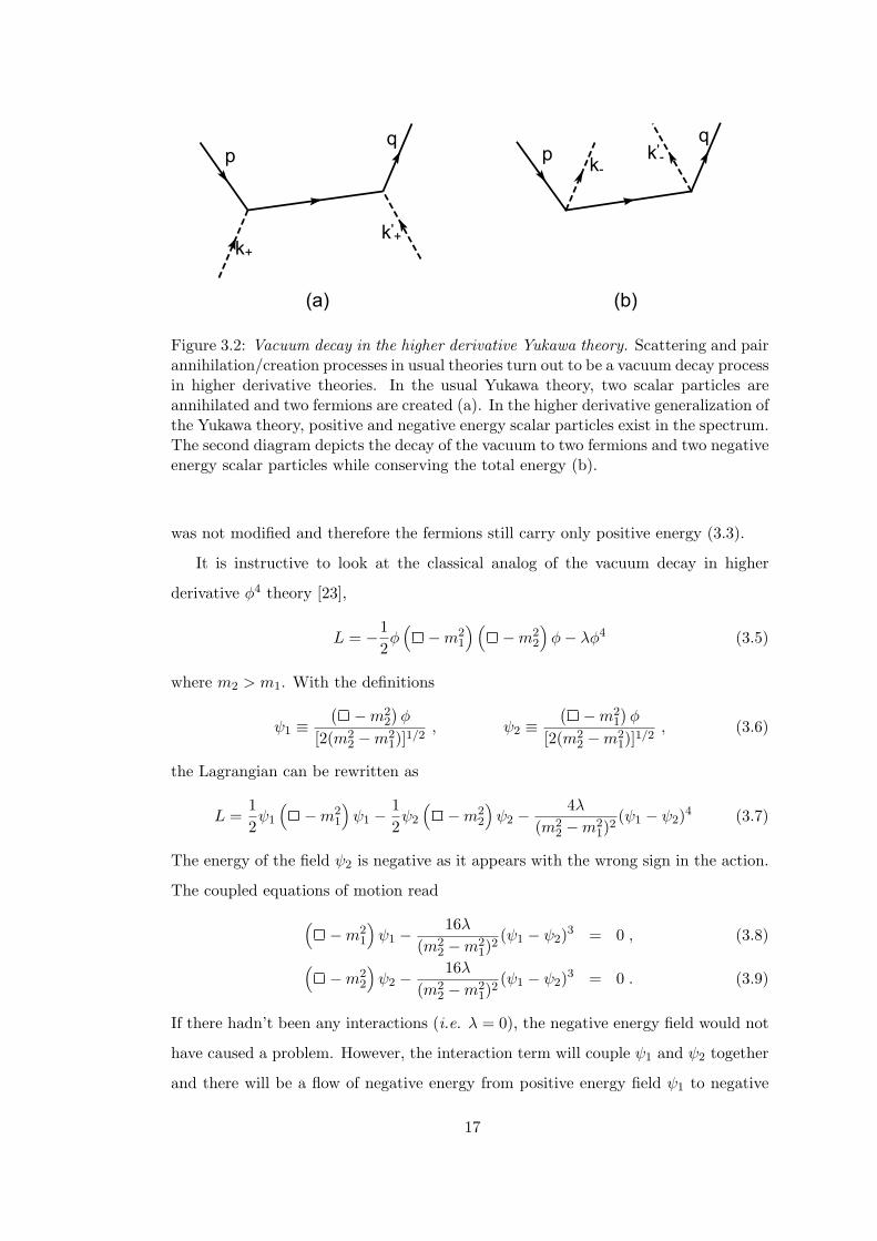
Figure 3.2: Vacuum decay in the higher derivative Yukawa theory. Scattering and pairannihilation/creation processes in usual theories turn out to be a vacuum decay processin higher derivative theories. In the usual Yukawa theory, two scalar particles areannihilated and two fermions are created (a). In the higher derivative generalization ofthe Yukawa theory, positive and negative energy scalar particles exist in the spectrum.The second diagram depicts the decay of the vacuum to two fermions and two negativeenergy scalar particles while conserving the total energy (b).

was not modified and therefore the fermions still carry only positive energy (3.3).

It is instructive to look at the classical analog of the vacuum decay in higher

derivative φ4 theory [23],

L = −12φ

(−m2

1

) (−m2

2

)φ− λφ4 (3.5)

where m2 > m1. With the definitions

ψ1 ≡( −m2

2

)φ

[2(m22 −m2

1)]1/2, ψ2 ≡

( −m21

)φ

[2(m22 −m2

1)]1/2, (3.6)

the Lagrangian can be rewritten as

L =12ψ1

(−m2

1

)ψ1 − 1

2ψ2

(−m2

2

)ψ2 − 4λ

(m22 −m2

1)2(ψ1 − ψ2)4 (3.7)

The energy of the field ψ2 is negative as it appears with the wrong sign in the action.

The coupled equations of motion read

(−m2

1

)ψ1 − 16λ

(m22 −m2

1)2(ψ1 − ψ2)3 = 0 , (3.8)

(−m2

2

)ψ2 − 16λ

(m22 −m2

1)2(ψ1 − ψ2)3 = 0 . (3.9)

If there hadn’t been any interactions (i.e. λ = 0), the negative energy field would not

have caused a problem. However, the interaction term will couple ψ1 and ψ2 together

and there will be a flow of negative energy from positive energy field ψ1 to negative

17

0.5 1 1.5 2 t0.5

11.5

22.53

Ψ1@tD

0.5 1 1.5 2 t0.0250.050.075

0.10.1250.150.175

Ψ2@tD

Figure 3.3: Numerical solutions of the higher derivative φ4 theory. Space homogeneous(i.e. ∇2ψ1 = ∇2ψ2 = 0) numerical solutions of the equations (3.8) and (3.9) with theset of initial conditions ψ1(0) = 0.1, ψ1(0) = 0, ψ2(0) = 0, ψ2(0) = 0 show that bothof the positive energy field ψ1 and negative energy field ψ2 increase exponentiallywithout bound. The small difference in the values of the two graphs is due to themass difference (i.e. mψ1 6= mψ2) of the two fields. These two graphs show howOstrogradskian instability takes place at the classical level.

energy field ψ2 by conserving the total energy. So the arbitrary excitation of the

fields means that the theory is not stable. This can be easily seen through numerical

solutions of equations (3.8) and (3.9) (Fig. 3.3).

A similar analysis of instability in interacting higher derivative systems was given

by Nesterenko. In [24] a damping term γ dqdt is added to the equation of motion of

the Pais-Uhlenbeck oscillator (see 2.42). Then it is shown that this damping term

contributes a decaying part to the positive mode oscillations whereas it contributes

an exponentially growing part to the negative mode oscillations. In another words,

the damping term behaves like a sink for the positive mode solutions while it behaves

like a source for the negative mode solutions. This result stems from the fact that

Hamiltonian is unbounded.

This negative energy problem is manifest in quantum theory through ghost states.

We can calculate the free field propagator for the Lagrangian (3.5),

G(p) =1

(m22 −m2

1)

(1

(p2 + m21)− 1

(p2 + m22)

). (3.10)

Due to the minus sign in (3.10), we immediately recognize that one of the particles in

the spectrum, m1 or m2, is a ghost. An important note is in order: This ghost is not

the same kind of the Faddeev-Popov ghosts which cancel with unphysical components

of the original fields; on the contrary, the ghost here exists on its own and it cannot

be cancelled or excluded from the theory in any way [25].

Another point is that in the equal mass (or equal frequency) limit, (3.10) diverges

18

and the Hamiltonian is no more diagonalizable, but “Jordan diagonalizable”, which

is similar to

1 1

0 1

. (3.11)

This Jordan matrix has only one eigenvector ∝

1

0

. Even though there are some

n× n Jordon diagonalizable matrices which have n eigenvectors, for a higher deriva-

tive theory which employes the Jordon matrix (3.11), an immediate criticism follows

stating that it is not possible to make a measurement in this theory where the Hamil-

tonian is Jordan diagonalized because there is not enough number of base vector to

span the whole Hilbert space.

3.2 Indefinite Metric Stratagem

In the previous chapter, we showed that half of the degrees of freedom contributes

negative energy to the Hamiltonian and quantization does not stabilize higher deriva-

tive theories (2.70). On the other hand, some people try to quantize the theory in a

different way.

It’s thought that one can treat the negative energy lowering operator as a positive

energy raising operator. So in contrast to the formalism given in (2.57, 2.58), they

[16] use

a |Ω〉 = 0 , (3.12)

b† |Ω〉 = 0 , (3.13)

with the usual commutation relations

[a, a†] = 1 = [b, b†] . (3.14)

Hence positive N+ and negative N− energy states can be produced from vacuum by

|N+〉 = a† |Ω〉 , (3.15)

|N−〉 = b |Ω〉 . (3.16)

Using the commutation relations (3.14), we find⟨N+|N+

⟩=

⟨Ω|Ω

⟩, (3.17)

⟨N−|N−

⟩= −

⟨Ω|Ω

⟩. (3.18)

19

Here the norm of the negative energy particles is negative. Furthermore, the reason

why we didn’t put 1 instead of⟨Ω|Ω

⟩will be seen below. It’s claimed that this

formalism is advantageous as it makes the energy positive valued. To examine this

claim, we can look at the vacuum expectation value of H from (2.70)

⟨Ω|H|Ω

⟩= k+

⟨Ω|a†a|Ω

⟩− k−

⟨Ω|b†b|Ω

⟩, (3.19)

= k+

⟨Ω|(aa† − 1)|Ω

⟩− k−

⟨Ω|b†b|Ω

⟩, (3.20)

= k+

⟨N+|N+

⟩− k+

⟨Ω|Ω

⟩− k−

⟨N−|N−

⟩, (3.21)

= k+

⟨Ω|Ω

⟩− k+

⟨Ω|Ω

⟩+ k−

⟨Ω|Ω

⟩. (3.22)

Here the energy seems to be positive valued. So this formalism renders positive norm

negative energy states into negative norm positive energy states. To preserve unitarity

of the S-matrix and to be able to make probabilistic interpretation, negative norm

states should be excluded from the physical sector. For this, a new definition of norm

in Hilbert space was proposed by means of an indefinite metric, but to date no one

was able to solve the problem in a consistent way.

Besides, there is another problem with this formalism which is at least as important

as the unitarity. If we solve (3.12) and (3.13) for the empty state wave function, we

get

Ω(Q1, Q2) = N exp

[− m

√1−4g

2(k−−k+)

(k+k−Q2

1 −Q22

)+ i√

gmQ1Q2

]. (3.23)

Unfortunately the wave function does not fulfill the normalizability condition (2.67)

this time. This means that we’re no longer doing quantum mechanics and we are not

able to obtain finite results from this theory. So it seems that there is no use of this

formalism.

3.3 Perturbative Approach

Higher derivative terms increase the dimension of the phase space and the number

of solutions irrespective of how they appear in the Lagrangian and this result is not

altered when higher derivatives are present only in the interaction part with small

coupling constants.

If higher derivative terms are gathered in the interaction part, then one can solve

20

the equations perturbatively by the ansatz [10, 26],

qpert(t) =∞∑

n=0

gnqn(t) . (3.24)

As an example, let us consider the Lagrangian [10]

L = −mg(1− g)2ω2

q2 +m

2q2 − mω2

2q2 (3.25)

for 0 < g < 1. Note that here the constant term in front of q2 is different from the

one in (2.42) for further convenience. The Euler-Lagrange equation for (3.25) reads

g(1− g)ω2

q(4) + q + ω2q = 0 . (3.26)

The solution is the same with (2.45), but the frequencies here are found as

k+ =ω√

1− gand k− =

ω√g

(3.27)

If we substitute the ansatz (3.24) into (3.26) and separate the terms with respect to

powers of g, we get the following system of equations

q0(t) + ω2q0(t) = 0 , (3.28)

q1(t) + ω2q1(t) = − 1ω2

q(4)0 (t) , (3.29)

... (3.30)

qn(t) + ω2qn(t) = − 1ω2

(q(4)(n−1) − q

(4)(n−2)

). (3.31)

This system of equations can be written in a more compact form

qk(t) = −ω2k∑

l=0

ql(t) . (3.32)

This is achieved by differentiating each equation and substituting it into the next

equation so that the fourth derivative terms on the right-hand side of the equations

are removed. If we multiply both sides of (3.32) by gk and sum over k, we obtain∞∑

k=0

gkqk(t) = −ω2∞∑

k=0

gkk∑

l=0

ql(t) . (3.33)

The left-hand side of (3.33) is qpert(t) from (3.24). Interchanging the order of summa-

tions on the right-hand side yields

qpert(t) = −ω2∞∑

l=0

ql(t)∞∑

k=l

gk (3.34)

= −ω2∞∑

l=0

ql(t)gl

1− g(3.35)

= − ω2

1− gqpert(t) . (3.36)

21

Hence we obtained qpert(t) by means of the perturbative ansatz and the Euler-Lagrange

equation without any reference to initial conditions.

Now notice that the term ω2

1−g in (3.36) is nothing but k2+. So we can conclude that

the perturbation theory does not follow from the original theory since it respects the

solutions with positive energy but discards the ones with negative energy. However,

there is a nonperturbative amplitude for the system to decay to the higher excitations

(i.e. Ostrogradskian instability). This eventually makes perturbation theory useless.

22

CHAPTER 4

VIABLE HIGHER DERIVATIVE THEORIES

In the previous chapter, it was shown that all nondegenerate higher derivative theories

suffer from Ostrogradskian instability irrespective of the form of the Lagrangian. On

the other hand, if the assumption of nondegeneracy, which is central for Ostrogradski’s

canonical formulation, is relinquished, then it may be possible to get a stable higher

derivative theory.

If the system is degenerate, this means that one cannot solve q(N) in terms of PN ,

q and the first N − 1 derivatives of q (see 2.4 and 2.15) and therefore the Hamiltonian

cannot be obtained by simply Legendre transforming the Lagrangian. Degeneracy

implies the presence of a continuous symmetry (or symmetries). This continuous

symmetry can be used to eliminate a dynamical variable by gauge fixing and this

yields constraints.

A simple rule to check the stability of a degenerate higher derivative theory was

given by Woodard [11]:

“If the number of gauge constraints is less than the number of unstabledirections in the canonical phase space then there is no chance for avoidingthe problem [of Ostrogradskian instability].”

The number of unstable directions increases with higher derivative terms, but any

continuous symmetry results fixed number of constraints. So constraints may stabilize

only the theories which contain some fixed number of higher derivative terms. For

example, the model of relativistic particle with a second derivative curvature term is

stable whereas it is not so if a third derivative torsion term is included.

23

4.1 Relativistic Particle with “Curvature” and “Torsion”

Relativistic particle with a higher derivative curvature term which was worked out by

Plyushchay [27] is the only hitherto known theory free of Ostrogradskian instability. In

order to see that the third order additional torsion term produces tachyonic (negative

mass) states, here we will make the calculations for the action of relativistic particle

with both curvature and torsion terms and then we will show that tachyonic states in

the mass spectrum disappear provided that the torsion term is excluded.

The second derivative curvature term in the Lagrangian is sometimes called “rigid-

ity” and also studied in the context of string theory. Polyakov [28] introduced a second

derivative term to the original Nambu-Goto action in order to give strings some kind

of rigidity so as to prevent the “creasing” (or “crumpling”) effect. In addition, rigidity

is introduced with higher derivative terms both in the theory of cosmic strings and

the theory of flexural vibrations of beams and rods in mechanical engineering [29].

The action of the relativistic particle of mass m with additional curvature and

torsion terms is given by [30]

S = −m

∫ds− α

∫k(s) ds− β

∫κ(s) ds , (4.1)

where ds2 = gµνdxµdxν ; k(s) =[(

d2xµ

ds2

)2]1/2

and κ(s) =[(

d3xµ

ds3

)2]1/2

are curvature

and torsion of the world curve of the particle, respectively, m is a constant in mass

dimensions, and α and β are dimensionless constants.

For the parametrization xµ = xµ(τ), we use

d

ds−→ dτ

ds

d

dτand ds2 =

(dxµ

dτ

)2dτ2 = x2dτ2 , (4.2)

to rewrite the action (4.1) in the form

S = −m

∫dτ√

x2 − α

∫dτ

((xx)2 − x2x2)1/2

x2− β

∫dτ

√x2 d

(xx)2 − x2x2, (4.3)

where

x ≡ dx

dτ, d = det(dρσ), dρσ = x(ρ) µx(σ)

µ , x(ρ) ≡ dρx

dτρ, ρ, σ = 1, 2, 3. (4.4)

As a digression, we may look at the nonrelativistic limit of the model of relativistic

particle with a curvature term. Here we will include the constant of speed of light c

in the action in contrast to (4.3) so as to make the limiting procedure more evident.

S = −mc

∫dτ√

x2 − αc

∫dτ

((xx)2 − x2x2)1/2

x2, (4.5)

24

Without loss of generality, we can take x0(τ) = cτ , x0(τ) = c, x0(τ) = 0 where the

“overdot” denotes the differentiation with respect to τ as defined in (4.2). The non-

relativistic limit of the first part of the action (4.5) is well known. The nonrelativistic

limit occurs when ~x2

c2¿ 1.

−mc√

x2 = −mc

√x0x0 − ~x~x = −mc

√c2 − ~x

2(4.6)

= −mc2

√

1− ~x2

c2= −mc2(1− 1

2~x

2

c2) = −mc2 +

12m~x

2. (4.7)

Obviously the first term has no effect on the equation of motion as it is just a constant

and the second term is the kinetic energy of a point particle.

As for the curvature term in (4.5), the nonrelativistic limit of it is as follows:

−αc((xx)2 − x2x2)1/2

x2= −αc

((x0x0 − ~x~x)2 − (x0x0 − ~x~x)(x0x0 − ~x~x))1/2

x0x0 − ~x~x(4.8)

= −αc((~x~x)2 − (c2 − ~x~x)(−~x~x))1/2

c2 − ~x~x(4.9)

= −αc

((~x~x)2

(c2 − ~x2)2

+~x

2

(c2 − ~x2)

)1/2

(4.10)

= −αc

((~x~x)2

1c4

1

(1− ~x2

c2)2

+ ~x2 1c2

1

(1− ~x2

c2)

)1/2

(4.11)

= −α

((~x~x)2

1c2

(1 + 2

~x2

c2

)+ ~x

2(1 +

~x2

c2

))1/2

(4.12)

= −α

(~x

2((~x~x)2

~x2c2

+ 1))1/2

= −α |~x| . (4.13)

In the step (4.12) we used the assumption(1 + ~x

2

c2

)≈

(1 + 2 ~x

2

c2

)≈ 1 and in the last

step we adopted (~x~x)2

~x2c2¿ 1. Thus the nonrelativistic limit of the curvature term gives

the magnitude of the acceleration of a point-like particle. Here notice that the result

in (4.13) is not a total derivative and it contributes higher derivative terms to the

equation of motion.

Going back to the main discussion of the relativistic model (4.3), the canonical

variables are defined according to (2.14)

q1 = x, q2 = x, q3 = x , (4.14)

p1 =∂L

∂x+

d

dτ

∂L

∂x+

d2

dτ2

∂L

∂x(3), (4.15)

p2 =∂L

∂x− d

dτ

∂L

∂x(3), (4.16)

25

p3 =∂L

∂x(3), (4.17)

where p3 is given explicitely by

pµ3 = β

√x2

(xx)2 − x2x2

√d

3∑

ρ=1

d3ρx(ρ)µ . (4.18)

Here dρσ is the matrix inverse to dρσ so that dρσ dσγ = δγρ .

Notice that the power of x(3) is one in the term√

d, whereas it is minus one in

the summation part. So the right-hand side of (4.18) is homogeneous of degree zero

and one cannot solve for x(3). This means that our model is singular and therefore

some constraints should be used for the Hamiltonization. The associated continuous

symmetry is invariance under reparametrizations

τ −→ f(τ) and xµ(τ) −→ x′µ(τ) ≡ xµ(f−1(τ)) (4.19)

It is easy to check that the action (4.3) is invariant under this reparametrization.

From (4.18) we can deduce three primary constraints:

(1)

φ 1 = p23 + β2(q2

2/g) = 0 , (4.20)(1)

φ 2 = p3q2 = 0 , (4.21)(1)

φ 3 = p3q3 = 0 , (4.22)

where g = (q2q3)2 − q22q

23 and the overscript “(1)” denotes that the constraint is “pri-

mary”. According to Dirac’s classification, primary constraints are the ones derived

directly from the conjugate momentum.

En route to quantization, we first examine the invariant Casimir operators in the

model. The angular momentum is given by

Mµν =3∑

α=1

(qαµpαν − qανpαµ) . (4.23)

Since our theory is invariant under the Poincare group of transformations, we consider

the following Casimir operators of the Poincare group:

C1 = p21 = p1µpµ

1 , (4.24)

C2 = W = −wµwµ =12MµνM

µνp21 − (Mµσpµ

1 )2 , (4.25)

where wµ = (1/2)εµνρσMνρpσ1 is the Pauli-Lubanski pseudovector. Here the mass cor-

responds to the Casimir operator (4.24) whereas the spin corresponds to the Casimir

operator (4.25).

26

If we go to the rest frame where pµ1 = (p0

1 = M, ~p1 = 0), then we have,

W = (p01)

2M12M12 = M2 C(SO(2))

2, (4.26)

where C(SO(2)) is the squared Casimir operator of the SO(2) group which is equal

to 2j2 [31] 1. The representations of the group of rotations on the plane SO(2) are

integers, half-odd-integers, and continuous values for spin j. The eigenvalues of the

Casimir operator W are

W = M2j2, M2 > 0, j ≥ 0 . (4.27)

The state vectors |ψ〉 are eigenvectors of the operators (4.24) and (4.25)

p21 |ψ〉 = M2 |ψ〉 , (4.28)

W |ψ〉 = M2j2 |ψ〉 . (4.29)

Here the constraint(1)

φ 1 (4.20) will give the wave equation. But we first fix the gauge

(recall the reparametrization invariance (4.19)) by q2q3 = 0 and subsequently the

constraint (4.20) becomes(1)

φ 1 = (p23q

23 − β2). Note that this is indeed the proper time

gauge, x0(τ) = τ , considering (4.14). So the wave function is given by

(1)

φ 1 |ψ〉 = (p23q

23 − β2) |ψ〉 . (4.30)

The left-hand side of (4.30) can be expressed in terms of the Casimir operators p21 and

W . According to the calculation done in the appendix of [30], we have

1− χ =W − (α

√m2 − p2

1 + |β|m√χ)2

β2p21

χ

1 + χ, (4.31)

where χ = β2/(p23q

23). So (4.30) becomes

(1− χ) |ψ〉 = 0 , (4.32)

which is equivalent to

[W − (α

√m2 − p2

1 + |β|m)2]|ψ〉 = 0 . (4.33)

1 We concluded this result in the rest frame but in fact the result is frame independent, becausethe subgroup of the Poincare group that leaves pµ invariant has the same structure in all frames. Thissubgroup is called the little group and in this case it’s a rotation group. So the representations of therotation group give the representations of the Lorentz group for a timelike state [32].

27

Substituting the operators (4.28) and (4.29) into (4.33) yields

M2j2 = (α√

m2 −M2 + |β|m)2 . (4.34)

To obtain the mass spectrum, we solve (4.34) for the ratio M2/m2

M2

m2=

α2(j2 + α2) + β2(j2 − α2)± 2 |β|√j2α2(j2 + α2 − β2)(j2 + α2)2

. (4.35)

Obviously tachyonic solutions are allowed in the spectrum. For example, if j = 0 then

(4.35) becomesM2

m2= 1− β2

α2, (4.36)

where tachyonic states appear if |β| > |α|.However, if we set β = 0 in (4.34); i.e., kill the torsion term in the action (4.1),

we end up with a positive valued mass spectrum of a relativistic particle with second

order curvature termM2

m2=

11 + j2/α2

. (4.37)

It’s also shown in [33] that the torsion term leads to tachyonic solutions. Thus the

only hitherto known higher derivative theory free of tachyons is the relativistic particle

with a curvature term.

4.2 Nonlocal Theories

Nonlocality is the case where objects or fields in different points of the spacetime inter-

act directly with each other without any mediator between them. Nonlocality appears

in diverse areas of physics such as quantum field theory, string theory, noncommuta-

tive geometry, regularization techniques and even cosmology (see references in [11]).

The point is that if a nonlocal theory can be represented as the limit of a sequence of

higher derivative theories, then the Ostrogradskian instability is unavoidable. String

theory for which such a representation is possible and nonlocal actions in which terms

such as q(t) and q(t+ τ) appear 2 hold this instability [10, 12]. Higher derivative limit

of a nonlocal theory can be reached if the action is analytic in derivatives.

As an illustration, consider the analytic higher derivative Lagrangian

L =12q2 − 1

2ω2q exp

(− g

ω2

d2

dt2

)q , (4.38)

2 These kind of equations are studied also by mathematicians under the name of delay differentialequations.

28

where g is real and (4.38) becomes the usual harmonic oscillator for g = 0. The

associated Euler-Lagrange equation is,

q = −ω2 exp

(− g

ω2

d2

dt2

)q . (4.39)

After imposing a solution of the form

q(t) = eiκωt , (4.40)

we obtain the equation

κ2 = e gκ2. (4.41)

Setting κ2 = a + ib yields

a + ib = egaeigb . (4.42)

Taking the square of both sides of (4.42) and solving for b yields

b = ±(e2ga − a2)1/2 . (4.43)

Substituting (4.43) into (4.42), for positive values of b we obtain

a = ega cos[g

(e2ga − a2

)1/2]

. (4.44)

For a large and positive, (4.43) and (4.44) become

b ≈ ega , (4.45)

a ≈ ega cos (gega) . (4.46)

The left-hand side of (4.46) is order of a whereas ega term exists in the right-hand

side. Hence the value of the cosine function should be very close to zero for (4.46) to

be valid. Since zeros of the cosine function are at (2N+1)2 π for N integer, we conclude

gega ∼ (2N + 1)2

π , (4.47)

b ∼ 1g

(2N + 1)2

π . (4.48)

Consequently we end up with

κ2 ∼ 1g

ln[1g

12(2N + 1)π

]± i

1g

12(2N + 1)π . (4.49)

There are infinitely many solutions due to the exponential term in the Lagrangian

(4.38), which is actually nothing but an infinite sequence of higher derivatives in

29

disguise. The energy will obviously be unbounded if we consider the Hamiltonian

which depends on infinite number of canonical momenta linearly.

There are runaway solutions in addition to the oscillations as the square root of κ2

has real and imaginary parts; nevertheless, these runaway solutions are not necessarily

associated with the Ostrogradskian instability 3.

On the other hand, if there is a nonanalytic dependence upon the derivative op-

erator, the theory may survive [10]. One example to it is

L[q] =12q2 − 1

2ω2q2 +

12g2ω2q

(ω2

d2/dt2 + ω2

)q , (4.50)

which the Lagrangian depends upon inverse differential operators.

Owing to the poles at d/dt = ±iω, higher derivative limit is not applicable. This

kind of nonlocality is obtained by integrating out one or more dynamical variables

and it does not change the stability or instability of the original theory. This sort

of nonlocality was named derived nonlocality [10]. The Lagrangian (4.50) is actually

derived from

L′[q, x] =12q2 − 1

2ω2q2 +

12x2 − 1

2ω2x2 − gω2xq . (4.51)

To derive (4.50) from (4.51) one first obtains the equation of motion for x

[d2

dt2+ ω2

]x = −gω2q =⇒ x = −gω2 1

d2/dt2 + ω2q . (4.52)

In (4.51), we can make the substitution x2 → −xd2xdt2

+ ddt(x

dxdt ) and can ignore the

ddt(x

dxdt ) term as it is a total derivative and does not contribute to the equataion of

motion. Hence, (4.51) can be written in the form

L′[q, x] =12q2 − 1

2ω2q2 − 1

2x

[d2

dt2+ ω2

]x− gω2xq . (4.53)

So it can be readily checked that substitution of (4.52) into (4.53) gives (4.50). Obvi-

ously there is neither negative energy solutions nor runaways since the original theory

is nothing but two coupled harmonic oscillators.

Therefore, if a nonanalytic dependence of the Lagrangian upon derivative operators

is present, we may have a viable higher derivative theory.

3 Recall that in section 3.1 we distinguished the Ostrogradskian instability and the instabilitycaused by unbounded potentials. The Ostrogradskian instability is associated with the runawaysolutions which take place if interactions are allowed. However, runaways due to unbounded potentialsmay appear in usual lower derivative theories even without any interaction.

30

CHAPTER 5

CONCLUSION

In this work, it is shown that all nondegenerate higher derivative theories suffer from

Ostrogradskian instability. There is no way to circumvent this problem since the

Hamiltonian of higher derivative theories is not positive valued and this result is

independent of the form of the Lagrangian.

In contrast to the case of the Hydrogen atom, quantization here does not remove

the instability. This is indeed expected because the emergence of Ostrogradskian in-

stability is due to the interaction between positive and negative energy modes (or

particles). The Ostrogradskian instability is manifest both at the classical and quan-

tum levels and it causes the solutions to become arbitrarily highly excited.

To date no one has been able to find a way to get rid of the negative energy

problem. It should be emphasized that we mean “truly” negative energy, not negative

frequency. It was also seen that quantizing a higher derivative theory in a somewhat

different way by reinterpreting the negative energy ladder operators seems to produce

a positive valued energy, however, negative norm states spring up this time. Also the

wave functions are not normalizable in this “wrongly” quantized theory.

When a higher derivative field theory is considered, we encounter the problem

of ghost particles with negative energies. Thus the decay of the vacuum into some

collection of positive and negative energy particles is allowed as the total energy is

conserved. We can conclude that scattering and pair annihilation/creation processes

in usual lower derivative theories turn to the vacuum decay process in higher derivative

theories. Hence, an unstable vacuum makes these theories useless.

The spectrum of higher derivative models include both positive and negative en-

ergy modes (or particles). However, the perturbative approach discards the negative

energy modes and therefore it becomes useless since there is always a nonperturbative

31

amplitude for the system to decay.

As for the degenerate case, the model of the relativistic particle with a higher

derivative curvature term is free of the Ostrogradskian instability. A simple rule

applies to check the stability of degenerate theories: The number of gauge constraints

should be more than the number of unstable directions in the canonical phase space.

Since the number of constraints due to a continuous symmetry is fixed, adding

more higher derivative terms increase the dimension of the phase space and also the

instable directions on it. We showed that third order derivate torsion term spoils the

stability of the model of the relativistic particle with a curvature term and in the

presence of a torsion term, we find negative energy tachyons in the spectrum.

Besides, an example is given for the derived higher derivative theories which are

obtained by integrating out one or more dynamical variables from the Lagrangian.

We have not touched the higher curvature gravity theories in this thesis, however,

studies in this area are still going on. For example, it is proposed that higher curvature

terms may mimic dark energy. The question of the stability of higher derivative

theories on anti-de Sitter spacetime seems to be an open problem.

32

REFERENCES

[1] A. D. Fokker, Z. Phys. 58, 386 (1929) ; F. Bopp, Ann. Physik 38, 345 (1940); B.Podolsky and P. Schwed, Rev. Mod. Phys. 20, 40, (1948); J. A. Wheeler and R.P. Feynman, Rev. Mod. Phys. 17, 157 (1945); 21, 425, (1949); A. E. S. Green,Phys. Rev. 73, 26 (1948).

[2] H. Euler, B. Kockel, Naturwissenschaften 23, 246 (1935); H. Euler, Ann. Phys.26, 398 (1936); W. Heisenberg, H. Euler, Z. Phys. 98, 714 (1936); J. Schwinger,Phys. Rev. 82, 664 (1951).

[3] M. Born, L. Infeld, Proc. Roy. Soc. A 144, 425, (1934).

[4] H. Weyl, Raum-Zeit-Materie, (1921), 4th ed. (Springer-Verlag, Berlin) [Englishtranslation Space-Time-Matter (Dover, New York), Chap IV; A. Eddington, TheMathematical Theory of Relativity, (1924), 2nd ed. (Cambridge University Press,London), Chap. IV]; K. S. Stelle, Gen. Rel. Grav. 9, 353 (1978).

[5] N. Moeller, B. Zwiebach, JHEP 0210 (2002) 034, hep-th/0207107.

[6] Stephan Didas, Higher Order Variational Methods for Noise Removal in Signaland Images, PhD Thesis, Saarland University, (October 2004).

[7] S. J. Linz, Am. J. Phys. 65 (6), (1997); S. J. Linz, Am. J. Phys. 66 (12), (1998);R. Eichhorn, S. J. Linz and P. Hanggi, Phys. Rev. E 58, 7151, (1998); J. C.Sprott, Am. J. Phys. 65 (6), (1997); H. P. W. Gottlieb, Am. J. Phys. 66 (10),(1998).

[8] M. Ostrogradski, Mem. Ac. St. Petersbourg VI 4, 385 (1850); E. T. Whittaker,Analytical Dynamics (1937), (Cambridge University Press, London, 1937), 4thedition, p.265.

[9] D. M. Gitman, I. V. Tyutin, Quantization of Fields with Constraints, (Springer-Verlag, Berlin, 1990).

[10] D. A. Elizer, R. P. Woodard, Nucl. Phys. B 325, 389 (1989).

[11] R. P. Woodard, Avoiding Dark Energy with 1/R Modifications of Gravity, astro-ph/0601672.

[12] R. P. Woodard, Phys. Rev. A 62, 052105 (2000).

[13] H.-J. Schmidt, Phys. Rev. D 49, 6354 (1994).

[14] P. A. M. Dirac, Can. J. Math. 2, 129 (1950); 3, 129 (1951); Lectures on QuantumMechanics (Yeshiva University, New York, 1964).

[15] D. M. Gitman, S. L. Lyakhovich, I. V. Tyutin, Soviet Phys. Journ. 26, 730 (1983).

33

[16] P. D. Mannheim, Phys. Rev. A 71, 042110 (2005), hep-th/0408104; Solution tothe Ghost Problem in Fourth Order Derivative Theories, hep-th/0608154

[17] C. G. Bollini, J. J. Giambiagi, Rev. Bras. Fis. 17, 14 (1987).

[18] A. Pais, G. E. Uhlenbeck, Phys. Rev. 79, 145 (1950).

[19] I. Ya. Aref’eva, L. V. Joukovskaya, JHEP 0510 (2005) 087, hep-th/0504200.

[20] S. Coleman, “Acausality” in Subnuclear Phenomena, ed. A. Zichichi, New York(1970).

[21] A. V. Smilga, Nucl. Phys. B 706, 598 (2005); Phys. Lett. B 632, 433 (2006).

[22] W. Greiner, Quantum Mechanics: Special Chapters, (Springer-Verlag, Berlin,1998).

[23] S. W. Hawking, T. Hertog, Phys. Rev. D 65, 103515 (2002).

[24] V. V. Nesterenko, Phys. Rev. D 75, 087703 (2007).

[25] D. A. Johnston, Nucl. Phys. B 297, 721 (1987).

[26] X. Jaen, J. Llosa, A. Molina, Phys. Rev. D 34, 2302 (1986).

[27] M. S. Plyushchay, Int. J. Mod. Phys. A 4, 3851 (1989).

[28] A. Polyakov, Nucl Phys. B 268, 406 (1986); G. German, Mod. Phys. Lett. A 6,1815 (1991).

[29] A. M. Chervyakov, V. V. Nesterenko, Phys. Rev. D 48, 5811 (1993).

[30] V. V. Nesterenko, J. Math. Phys. 32, 3315 (1991).

[31] A. O. Barut, R. Raczka, Theory of Group Representations and Applications,(Polish Scientific Publishers, Warszawa, 1977).

[32] L. H. Ryder, Quantum Field Theory, (Cambridge University Press, 1996), 2nded., p. 62.

[33] M. S. Plyushchay, Nucl. Phys. B 389, 181 (1993).

34