VI Wall-Bounded Turbulence

(A) The Navier-Stokes Equation in Bounded Domains

Before we can discuss turbulence in the presence of walls, we must first review some background

material on the solution of the Navier-Stokes equations in bounded domains. For an excellent

general discussion, we recommend

R. Teman, Navier-Stokes Equations: Theory and Numerical Analysis (North-Holland,

Amsterdam, 1984)

This subject might seem to be rather cut and dried but there are — amazingly — still many

confusions and controversies being discussed in the literature! There seems to be a great deal of

misunderstanding, in particular, of the proper boundary conditions for pressure and vorticity.

For example, the recent paper

D. Rempfer, “On the boundary conditions for incompressible Navier-Stokes prob-

lems,” Applied Mechanics Reviews 59 107-125 (2006)

extensively reviews the literature and points out many papers that still debate the “correct”

b.c. for pressure and vorticity! In fact, this should not be a matter of controversy, as there

are rigorous mathematical resolutions of those issues in the literature. There are open issues

about certain numerical schemes for solving the incompressible Navier-Stokes equation, which

we shall discuss briefly, but for the continuum equations the issues seem to be fully resolved.

Let us first discuss the appropriate boundary condition on the velocity u. It may seem “obvious”

that this should be the stick boundary condition (or no-slip b.c.)

u|!! = 0

on a motionless boundary !!, or, more generally,

u(x, t) = uB(x, t), (x, t) ! !!(t)

1

if the boundary is moving with velocity uB(x, t) at point (x, t). As a matter of fact, this issue

was long debated in the scientific community, going back to D. Bernouli and L. Euler in the

18th century. For an interesting historical discussion, see:

“Note on the Conditions at the Surface of Contact of a Fluid with a Solid Body,”

in Modern Developments in Fluid Dynamics, composed by the Fluid Motion Panel

of the Aeronautical Research Committee and Others, ed. S. Goldstein (Clarendon

Press, Oxford, 1938), reprinted by Dover, 1965; vol. II, pp. 676-680.

Many workers in the 18th and 19th century believed that there was a slip at the wall, so that the

fluid velocity at the wall and the velocity of the wall itself would disagree, perhaps substantially.

Navier proposed on the basis of a molecular argument that the slip velocity at the wall, "us,

should satisfy

"us = #s!u!n (")

for an appropriate length-scale #s. Experiments carried out in the 19th century by Stokes,

Whetham, Couette and others, however, showed no evidence of slip. Maxwell in 1879 used

kinetic theory to argue that for a solid-gas interface

#s#= #mf

where #mf is the mean-free length and thus |"us| $| u| (except possibly in a very rare gas,

or Knudsen gas). We now know that Maxwell’s conclusion is correct and that for macroscopic

fluid systems, slips at boundaries are generally very small. This is verified not only by many

experiments, but also by much recent theoretical and numerical work. For gases see

S. Shen et al., “A kinetic-theory based first-order slip boundary condition for gas

flow,” Phys. Fluids 19 086101 (2007)

and for more general fluids

C. Denniston and M. O. Robbins, “General continuum boundary conditions for

miscible binary fluids from molecular dynamics simulations,” J. Chem. Phys. 125

2

214102 (2006)

In the case of simple liquids, Navier’s law is a good approximation with #s#= #c, the correlation

length in the liquid. Thus, for macroscopic fluid flows, we see that slip velocities are generally

quite small and can be set = 0.

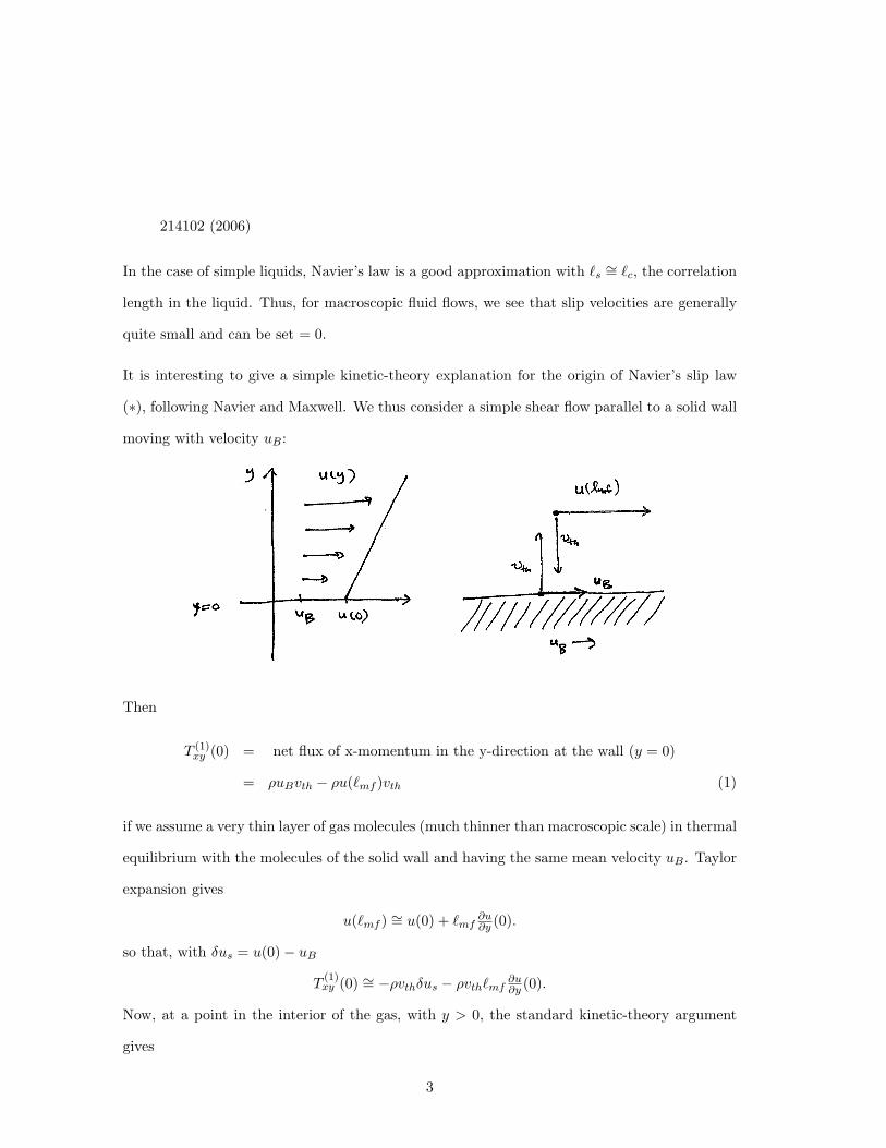
It is interesting to give a simple kinetic-theory explanation for the origin of Navier’s slip law

("), following Navier and Maxwell. We thus consider a simple shear flow parallel to a solid wall

moving with velocity uB:

Then

T (1)xy (0) = net flux of x-momentum in the y-direction at the wall (y = 0)

= $uBvth % $u(#mf )vth (1)

if we assume a very thin layer of gas molecules (much thinner than macroscopic scale) in thermal

equilibrium with the molecules of the solid wall and having the same mean velocity uB. Taylor

expansion gives

u(#mf ) #= u(0) + #mf!u!y (0).

so that, with "us = u(0)% uB

T (1)xy (0) #= %$vth"us % $vth#mf

!u!y (0).

Now, at a point in the interior of the gas, with y > 0, the standard kinetic-theory argument

gives

3

T (1)xy (y) = $u(y % #mf )vth % $u(y + #mf )vth

#= %2$#mfvth!u

!y(y)

= %%!u

!y(y) (2)

with shear viscosity % #= %2$#mfvth.

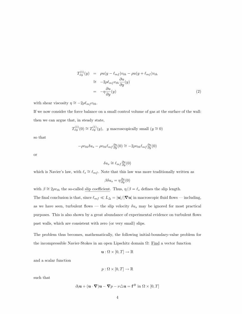
If we now consider the force balance on a small control volume of gas at the surface of the wall:

then we can argue that, in steady state,

T (1)xy (0) #= T (1)

xy (y), y macroscopically small (y #= 0)

so that

%$vth"us % $vth#mf!u!y (0) #= %2$vth#mf

!u!y (0)

or

"us#= #mf

!u!y (0)

which is Navier’s law, with #s#= #mf . Note that this law was more traditionally written as

&"us = % !u!y (0)

with & #= 2$vth the so-called slip coe"cient. Thus, %/& = #s defines the slip length.

The final conclusion is that, since #mf $ L" = |u|/|!u| in macroscopic fluid flows — including,

as we have seen, turbulent flows — the slip velocity "us may be ignored for most practical

purposes. This is also shown by a great abundance of experimental evidence on turbulent flows

past walls, which are consistent with zero (or very small) slips.

The problem thus becomes, mathematically, the following initial-boundary-value problem for

the incompressible Navier-Stokes in an open Lipschitz domain !: Find a vector function

u : !& [0, T ] ' R

and a scalar function

p : !& [0, T ] ' R

such that

!tu + (u · !)u%!p% '(u = fB in !& [0, T ]

4

! · u = 0 in !& [0, T ]

u(x, 0) = u0(x) in !

u(x, t) = 0 in !!& [0, T ]

The body-force fB and initial condition u0 are given as functions on ! & [0, T ] and on !,

respectively. We consider here the problem with stationary boundaries and stick velocities

(u = 0) in the boundary !!. The problem with moving boundaries and non-zero velocities on

the boundary can be handled by similar methods. For example, see

R. Salvi, “The exterior non-stationary problem for the Navier-Stokes equations in

regions with moving boundaries,” J. Math. Soc. Jap. 42 495-509 (1990)

The standard mathematical theory of Leray weak solutions of the problem with stationary

boundaries and stick conditions is in terms of the Hilbert space

H = {u ! L2(!, Rd),! · u = 0,u · n|!! = 0}

with n the outward-pointing unit normal on !!. This set of fields has finite energy, are in-

compressible (in distribution sense) and satisfy the condition of no-flow through the boundary.

Another important space, of greater smoothness, is

V = {u ! H1(!, Rd),! · u = 0,u|!! = 0}

which satisfy also!! |!u|2 ddx < +), incompressibility, and the full stick conditions u = 0 at

the boundary !!. The dual space

V ! * H"1(!, Rd)

is a space of divergence-free distributions that also plays a role in the Leray theory.

By projecting the Navier-Stokes equation onto the space H, one obtains the Leray weak form:

dudt + B(u,u) + 'Au = fB (")

Au + %P(u

B(u,u) = P ((u · !)u)

where P is the Helmholtz-Leray projection from L2(!, Rd) onto H, given by a Helmholtz

decomposition theorem (see e.g. Theorem I. 1.5 in Temam, 1984). For simplicity we have

5

assumed that fB = P fB, that is, that ! · fB = 0 and that fB · n = 0 on !!. It is known that

A : V ' V !

and, for dimension d , 4,

B : V & V ' V !.

Thus, the equation (") makes sense in the space V !, interpreted weakly, that is, we seek

u ! L2(0, T ;V ), dudt ! L1(0, T ;V !)

such that

-dudt + B(u,u) + 'Au% fB,!. = 0

for all ! ! V, with also

u(0) = u0.

Here it is assumed that fB ! L2(0, T ;V !) and u0 ! H.

The main theorem of the subject is that at least one solution exists to the above problem, with,

furthermore,

u ! L#(0, T ;H)

and u weakly continuous from [0, T ] into H, i.e. t /' (u(t),!) is a continuous function for all

! ! H. For example, see Theorem III. 3.1 of Temam (1984). It is noteworthy here that the

initial conditions u0 need not satisfy the full stick boundary conditions, but only the condition

of no-flow through the boundary. Nevertheless, at any positive time t > 0, the solution u(t) ! V

and thus satisfies the stick conditions. This shows that, in general, there will be a discontinuity

in the solution u(t) at the initial instant t = 0 at the boundary !!, with

n& u 0= 0 at t = 0 on !!

and

u = 0 at t > 0 on !!.

It is only for specially-prepared initial data that the Navier-Stokes solution can be smooth up

to t = 0. For a full discussion of these issues, we refer to

R. Temam, “Behavior at time t = 0 of the solutions of semi-linear evolution equa-

6

tions,” J. Di#. Eq. 43 73-92 (1982)

and, for a recent pedagogical discussion,

R. Temam, “Suitable initial conditions,” J. Comp. Phys. 218 443-450 (2006).

These papers discuss not only the incompressible Navier-Stokes equation but also other similar

parabolic problems, such as the linear heat equation. In general, compatibility conditions are

required on the initial data, in order to guarantee a given degree of smoothness up to time

t = 0. The first compatibility condition on u0 is that, in addition to u0 ! H, also

u0 ! H1(!, Rd) and u0 = 0 on !!

which is equivalent to requiring that

u0 ! V .

This condition is necessary and su"cient to have a strongly continuous solution, u ! C(0, T ;V ).

To give even more smoothness, the next-order condition or so-called second compatibility

condition is that

dudt

"""t=0

! V ,

or equivalently that

B(u0,u0) + 'Au0 % fB0 ! V .

In order to express this condition more transparently, we shall use the definition of Leray

projection in terms of the Helmholtz decomposition to write

B(u0,u0) + 'Au0 = (u0 · !)u0 % '(u0 %!p0 (()

where p0 is the solution of the Newmann problem#$%

$&

(p0 = !uoi!xj

!uoj

!xi

!p0!n = n · ('(u0)

(")

We have assumed, for simplicity, that fB0 ! V and already satisfies the stick condition at !!.

Because of the choise of p0, both sides of (() are divergence-free and have zero normal component

at the boundary !!. Thus, the second compatibility condition that B(u0,u0) + 'Au0 ! V

7

reduces to the condition that also the tangential component must vanish at the boundary, i.e.

that

n& [(u0 · !)u0 % '(u0 %!p0] = 0 on !!

or, since u0 = 0 on !!,

n& ['(u0 + !p0] = 0 on !!.

This is the simplest, most explicit form of the second compatibility condition for the Navier-

Stokes equation.

The above discussion implicitly answers the question about the proper boundary conditions for

pressure in the Navier-Stokes equation. We may apply the above arguments to any time t > 0,

with u(t) then playing the role of the initial condition u0. The introduction of the pressure by

the Leray projector implies that we may take p to solve the Neumann problem#$%

$&

(p0 = !ui!xj

!uo!xi

!p!n = n · ('(u)

(N)

However, if the Navier-Stokes solution is smooth in the region !& [t, T ], then the 2nd compat-

ibility condition implies that also

n& ['(u + !p] = 0 on !! (T ).

From this we can see that p satisfies also a suitable Dirichlet problem obtained by integrating

the above equation around the boundary. In general, the solution of these two elliptic problems

for p — the Neumann problem and the Dirichlet problem — would not have to coincide, for

an arbitrarily selected u and p. However, here (u, p) are in a special relationship, as a smooth

solution of the Navier-Stokes equation. In this case, compatibility requires that the Neumann

and Dirichlet pressures are exactly the same!

We emphasize that these facts have nothing to do with the possible occurence of singularities

in finite time for the 3D Navier-Stokes equation. Smooth solutions of the type considered

(up to the boundary and the initial time t) are guaranteed to exist in 2D and in 3D at low

Reynolds numbers. Even in 3D at high Reynolds number, the singularities — if any exist — are

8

confined to a zero-measure set, at most 1-dimensional in spacetime. Away from this singular

set, the Navier-Stokes solution is smooth up to the boundary !! of the domain and at each

positive time t > 0. The data u(t) has been “prepared” by the prior evolution so that all the

compatibility conditions are automatically satisfied at time t > 0, including the condition (T )

on the tangential pressure gradient at the boundary. As we shall see next, this condition has,

in fact, an important physical significance, as it is directly related to the generation of vorticity

at the boundary.

Vorticity dynamics in domains with boundaries

Given a solution of the Navier-Stokes equation (u, p), we know that the curl " = ! & u will

satisfy the Helmholtz vorticity equation

(!t + u · !)" = (" · !)u + '(" + !& fB

or

!t" = !& (u& " % '!& " + fB)

which may be written in conservation form as

!t)i + !j$ji = 0

with

$ij = ui)j % uj)i + '(!"i!xj

% !"j

!xi) + *ijkfB

k .

If we integrate the vorticity conservation law over the flow domain, then we obtain by the

divergence theorem

ddt

!! )id3x =

!!! $ijnjdA

where n is the outward-pointing unit normal. This suggests that we can interpret

#i + $ijnj

as a local vorticity source density at the wall. Because of the antisymmetry of $ij , we see that

n · # = 0

consistent with our earlier conclusion that, for stick b.c., n·" = 0. If we assume that n&fB = 0,

then we can simplify the above expression as

9

+i = '(!"i!xj

% !"j

!xi)nj

using both n · u = 0 and n · " = 0, or

# = %n& '(!& ").

It is sometimes preferable to use instead the inward - pointing unit normal n! = %n, so that

instead

# = n! & '(!& ").

The above argument is not entirely satisfactory, since we obtained only an integral formula

ddt

!! )id3x =

!!! +idA

and this does not permit an unambiguous identification of # as a local vorticity source. A better

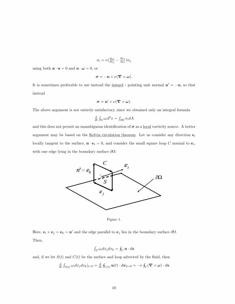
argument may be based on the Kelvin circulation theorem. Let us consider any direction ei

locally tangent to the surface, n · ei = 0, and consider the small square loop C normal to ei,

with one edge lying in the boundary surface !!:

Figure 1.

Here, ei & ej = ek = n! and the edge parallel to ej lies in the boundary surface !!.

Then,!S )idxjdxk =

'C u · dx

and, if we let S(t) and C(t) be the surface and loop advected by the fluid, then

ddt

!S(t) )idxjdxk|t=0 = d

dt

'C(t) u(t) · dx|t=0 = %'

'C(!& ") · dx

10

We see that the bottom segment parallel to ej is stationary in the surface (because of the stick

conditions) and that it contributes a term

%'!C$!!(!& ")jdxj

to the time-derivative of the flux!S )idA. We therefore identify

+i = %'(!& ")j

or, for any direction,

# = n! & '(!& ")

in agreement with our earlier finding. The above argument also reveals the precise meaning

of the “vorticity source density” #. If one considers any loop C with part of its length in

the boundary !!, then the contribution of the boundary segment to the time-derivative of the

vorticity flux through C is given by!C$!! # · (t& n!)ds

where t is the unit tangent vector along the curve C, for a specified orientation. With this

convention the flux is measured in the direction to the righthand side of the curve C as one

moves along it, i.e. || to t& n!.

The expression that we have derived for the “vorticity source density”

# = n! & '(!& ")

is the same as that obtained by

F. A. Lyman, “Vorticity production at a solid boundary,” Appl. Mech. Rev. 43

157-158 (1990)

These seems, however, to be some controversy about this result! It has been argued by

J. Z. Wu and J. M. Wu, “Interaction between a solid surface and a viscous com-

pressible flow field,” J. Fluid Mech. 254 183-211 (1993); “Vorticity dynamics on

boundaries,” Adv. in Appl. Mech. 32 119-275 (1996)

that Lyman’s prescription (and ours!) is incorrect and they suggest instead that

11

#Wu = ' !"!n = '(n · !)"

with outward-pointing normal n. However, this prescription seems to us based on fallacious

arguments, whereas our derivation from the Kelvin Theorem is particularly straightforward.

We note furthermore that # ought to lie parallel to vorticity vectors generated within the

boundary surface and thus satisfy n&# = 0. While Lyman’s prescription satisfies this condition,

n& #Wu 0= 0 in general!

Further insight and simplification can be obtained if one uses the Navier-Stokes momentum

balance

Dtu = %!p% '!& "

which can be solved to give

%'!& " = !p + Dtu

and thus

# = %n& '(!& ") = n& (!p + Dtu)

This form of the vorticity source density was first derived by

M. J. Lighthill, “Introduction: Boundary Layer Theory” in Laminar Boundary The-

ory, L. Rosenhead, ed. (Oxford University Press, Oxford, 1963), pp.46-113.

B. R. Morton, “The generation and decay of vorticity,” Geophys. Astrophys. Fluid

Dyn. 28 277-308 (1984)

who obtained the terms from the tangential pressure gradient and the tangential boundary

acceleration, respectively. Note that the above derivation was based on precisely the 2nd

compatibility relation (T ) for the Navier-Stokes solution, generalized to the case of a moving

boundary. This result reveals that the 2nd compatibility condition has a very fundamental

significance related to the generation of vorticity at a boundary. The term identified by Morton,

n& (Dtu), contributes only if the boundary is accelerating, either continuously or impulsively.

If we restrict our attention to uniformly moving ( or stationary) boundaries, then we recover

the original Lighthill (1963) result

12

# = n& (!p) = %n! & (!p).

This formula has several remarkable implications. First, one can see that the generation of

vorticity is essentially inviscid and does not vanish in the limit as ' ' 0. Second, the generated

vortex lines on the surface !! ought to tend to be parallel to the isobars, or lines of constant

pressure p. E.g. the following plot from the paper

J.-G. Liu, J. Liu, and R. L. Pego, “Stable and accurate pressure approximation for

unsteady incompressible flow,” J. Comp. Phys. 229 3428–3453 (2010)

shows vortex lines and pressure contours at the wall for a driven cavity flow:0 0.2 0.4 0.6 0.8 10

0.2

0.4

0.6

0.8

1 !5 !5

!5

!4

!4

!4

!3

!3

!3

!3

!2

!2

!2

!2

!2

!2

!2!2

!1

!1

!1

!1!1

!0.5

!0.5

!0.5

!0.5

!0.5

!0.5

0

0

0

0

0

0 0

0.5

0.5

0.5

0.5

0.5

0.5

0.5

1

1

1

1

1

1

1

1

1

2

2

2

2

2

2

2

23

3

3

3

3

33

0 0.2 0.4 0.6 0.8 10

0.2

0.4

0.6

0.8

1

!0.002

00.02

0.020.02

0.05

0.05

0.05

0.05

0.07

0.07

0.07

0.07

0.07

0.09

0.09

0.09

0.09

0.11

0.110.11

0.110.120.17

0 0.2 0.4 0.6 0.8 10

0.2

0.4

0.6

0.8

1!5 !5

!5

!4

!4

!4

!3

!3!3

!3

!2

!2

!2

!2

!2

!2

!2!2!1

!1

!1 !1

!1

!0.5

!0.5

!0.5

!0.5

!0.5

!05

0

0

0

00

0 0

0.5

0.5

0.5

0.5

0.5

0.5 0.5

1

1

1

11

1

1

1

1

2

2

2

2

2

22

2

23

3

3

3

3

3

3

0 0.2 0.4 0.6 0.8 10

0.2

0.4

0.6

0.8

1

!0.002 0

0.02

0.02

0.02

0.05

0.05

0.05

0.05

0.07

0.07

0.07

0.07

0.07

0.09

0.09

0.09 0.09

0.11

0.11

0.11

0.11 0.12

Fig. 8. Driven cavity, m ! 1=1000. P1/P1 with 8192 P1 elements (dof = 4225) for each variable. hmin ! 0:00594, hmax ! 0:0397;Dt ! 0:006; T ! 50. Top: (3,2)SC scheme. Bottom: (3,2) PA scheme. From left to right: vorticity contour plots, pressure contour plots.

0 0.5 1 1.5 2 2.5 3!0.5

0

0.5

S

X0 0.5 1 1.5 2 2.5 3

!0.5

0

0.5

S

X

Fig. 9. Backward-facing step. m ! 1=100. P1/P1 with 6640 P1 elements (dof = 3487) for each variable. hmin ! 0:00783; hmax ! 0:116, Dt ! 0:006; T ! 20.X=S ! 2:84. Left: (3,2) SC scheme. Right: (3,2) PA scheme.

0 1 2 3 4 5 6 7 8 9 10!0.5

0

0.5

X3

X1 X2

S

0 1 2 3 4 5 6 7 8 9 10!0.5

0

0.5

S

X3

X1 X2

Fig. 10. Backward-facing step. m ! 1=600. 1700 P2 elements (dof = 3925) for each variable. hmin ! 0:0186; hmax ! 0:334, Dt ! 0:003; T ! 120. Top: (3,2) SCscheme, X1=S ! 8:86; X2=S ! 15:5; X3=S ! 9:9. Bottom: (3,2) PA scheme, X1=S ! 8:86; X2=S ! 15:55, X3=S ! 9:9.

3446 J.-G. Liu et al. / Journal of Computational Physics 229 (2010) 3428–3453

Although the vortex source vector # is instantaneously tangent to the pressure isolines, the

vorticity vector " is a dynamical quantity which includes contributions both from the instan-

taneous source and from the evolution of past values.

For a review of these issues with many references to the literature, see

J. Z. Wu & J. M. Wu, “Boundary vorticity dynamics since Lighthill’s 1963 article:

review and development,” Theoret. Comput. Fluid Dyn. 10 459-474 (1998).

Of course, these authors defend the prescription #Wu!!!

A final remark is that the Constantin-Iyer stochastic formulation of incompressible Navier-

Stokes has been recently generalized to domains with boundaries, in

13

P. Constantin & G. Iyer, “A stochastic-Lagrangian approach to the Navier-Stokes

equations in domains with boundary,” Ann. Appl. Probab. 21 1466–1492 (2011)

and yields some new insight into the generation of vorticity at walls. The major di#erence

is that now stochastic Lagrangian trajectories moving backward in time can hit the domain

boundary !D before reaching the initial time t0 = 0, as illustrated here:

1470 P. CONSTANTIN AND G. IYER

3. The formulation for domains with boundary. In this section we describehow (2.3)–(2.5) can be reformulated in the presence of boundaries. We begin bydescribing the difficulty in using the techniques from [11] described in Section 2.

Let D ! Rd be a domain with Lipschitz boundary. Even if we insist u = 0 onthe boundary of D, we note that the noise in (2.3) is independent of space andthus, insensitive to the presence of the boundary. Consequently, some trajectoriesof the stochastic flow X will leave the domain D and for any t > 0, the map Xt

will (surely) not be spatially invertible. This renders (2.7) meaningless.In the absence of spatial boundaries, equation (2.7) dictates that !(x, t) is de-

termined by averaging the initial data over all trajectories of X which reach x attime t . In the presence of boundaries, one must additionally average the boundaryvalue of all trajectories reaching (x, t), starting on "D at any intermediate time(Figure 1). As we will see later, this means the analogue of (2.7) in the presenceof spatial boundaries is a spatially discontinuous process. This renders (2.6) mean-ingless, giving a second obstruction to using the methods of [11] in the presenceof boundaries.

While the method of random characteristics has the above inherent difficulties inthe presence of spatial boundaries, equation (2.8) is exactly the Kolmogorov Back-ward equation ([31], Section 8.1). In this case, an expected value representation inthe presence of boundaries is well known. More generally, the Feynman–Kac ([31],Section 8.2) formula, at least for linear equations with a potential term, has beensuccessfully used in this situation. A certain version of this method (Section 3.1),without making the usual time reversal substitution, is essentially the same as themethod of random characteristics. It is this version that will yield the natural gen-eralization of (2.3)–(2.5) in domains with boundary (Theorem 3.1). Before turningto the Navier–Stokes equations, we provide a brief discussion on the relation be-tween the Feynman–Kac formula and the method of random characteristics.

3.1. The Feynman–Kac formula and the method of random characteristics.Both the Feynman–Kac formula and the method of random characteristics have

FIG. 1. Three sample realizations of A without boundaries (left) and with boundaries (right).

In the case without boundaries, the Constantin-Iyer representation can be stated as

u(x, t) = P!xA0t (x) · u0

(A0

t (x))

(CI)

where the stochastic trajectories solve

dAst = u(As

t , s)ds +1

2' dW(s), s < t; Att = x,

the overline () is average over the Brownian motions, and P is the Leray projection. Integrating

the variable x in (CI) over a loop C yields the stochastic Kelvin theorem previously discussed.

In the presence of a boundary this formula is modified as follows:

u(x, t) = P!xA#t(x)t (x) · w

(A#t(x)

t (x), ,t(x))

(CI")

where ,t(x) is the backward exit time, or the time at which the stochastic trajectory leaving x

at time t reaches the space-time boundary. The space-time boundary value w is

w = u0 on D & {0},

14

the same as before, while

w = !- on !D & [0, t],

for a scalar function which solves the equation

!t- + (u · !)-% '(- +12|u|2 % p = c(t), -(0) = c0.

It is interesting that any spatial constants c(t) and c0 can be employed in this equation, and also

any boundary conditions for - on !D. Any such choice yields the same pressure gradient !p

and, substituted into (CL"), yields the Navier-Stokes solution with “stick” or zero-Dirichlet

boundary conditions (u = 0) at the wall! This representation is a generalization to incom-

pressible Navier-Stokes equation in a bounded domain of the Kuzmin-Oseledets formulation of

incompressible Euler equation. See

G. A. Kuzmin, “Ideal incompressible hydrodynamics in terms of the vortex momen-

tum density,” Phys. Lett. A 96 88–90 (1983)

V. I. Oseledets, “On a new way of writing the Navier-Stokes equation. The Hamil-

tonian formalism,” Commun. Moscow Math. Soc (1988); Russ. Math. Surveys 44

210–211 (1988).

In this formalism, the field p(x, t) defined by (CI") without the Leray projection P is termed

the “vortex momentum density” and u = p%!- = Pp.

Some remarks on numerical boundary conditions

Although the issue of boundary conditions for the continuum Navier-Stokes equation seems

settled, many interesting and important issues remain for numerical solution methods. For

example, see the article of Rempfer (2006) and Liu, Liu & Pego (201) for references to the

literature. Some common methods, such as the projection method, do not approximate the

pressure well near the wall in a boundary layer. See

R. Temam, “Remark on the pressure boundary condition for the projection method,”

Theoret. Comput. Fluid Dyn. 3 181-184 (1991)

15

There are also important issues about the boundary conditions for the Helmholtz equation in

the vorticity formulation of the Navier-Stokes equation. For this, see

J.-Z. Wu, H.-Y. Ma and M. D. Zhou, Vorticity and Vortex Dynamics (Springer,

Berlin, 2006), Section 4.5 “Vorticity-Based Formulation of Viscous Flows Problem”

J. -Z. Wu et al. “Dynamic vorticity condition: theoretical analysis and numerical

implementation,” Int. J. Num. Math. Fluids 19 905-938 (1994)

The di"culty is that the proper physical boundary conditions are the stick conditions on the

velocity:

u|!! = 0

and the velocity is nonlocally related to the vorticity ". Given the vorticity satisfying !·" = 0,

one must solve the problem

!& u = ", ! · u = 0, u|!! = 0

to determine u. This corresponds to the elliptic Poisson problem %(u = !&" with Dirichlet

b.c. The boundary conditions for " are inherently nonlocal and global and, without some

approximation, cannot be formulated as standard local conditions.

Finally, we remark that the Constantin-Iyer stochastic representation of the viscous Helmholtz

equation

!t" + (u · !)" = (" · !)u + '("

can be easily generalized to domains with boundaries, by taking

"(x, t) = (!A#t(x)t (x))%"1"(A#t(x)

t (x), ,t(x))

where the function " is defined simply to coincide with " = !&u on the space-time boundary

(D&{t = 0})2(!D&{t > 0}). This representation thus has the same practical problem as does

the standard PDE formulation of constructing the proper boundary values on the vorticity to

correspond to stick conditions on the velocity.

16