vhdl implementation of cordic algorithm for wireless …19532/fulltext01.pdf · vhdl implementation...
TRANSCRIPT

VHDL implementation of CORDIC algorithmfor wireless LAN
Master thesis performed in Electronics Systems by
Anastasia Lashko,
Oleg Zakaznov
LiTH−ISY−EX−3515−2004
Linköping, 2004

VHDL implementation of CORDIC algorithmfor wireless LAN
Master thesis in Electronics Systems
at Linköping Institute of Technology
by
Anastasia Lashko,Oleg Zakaznov
LiTH−ISY−EX−3515−2004
Supervisor: Kent Palmkvist
Examiner: Kent Palmkvist
Linköping, 20th of February, 2004

Avdelning, InstitutionDivision, Department
Institutionen för systemteknik581 83 LINKÖPING
DatumDate2003−02−20
SpråkLanguage
RapporttypReport category
ISBN
Svenska/SwedishX Engelska/English
LicentiatavhandlingX Examensarbete
ISRN LITH−ISY−EX−3515−2004
C−uppsatsD−uppsats
Serietitel och serienummerTitle of series, numbering
ISSN
Övrig rapport____
URL för elektronisk versionhttp://www.ep.liu.se/exjobb/isy/2004/3515/
TitelTitle
VHDL Implementation of CORDIC Algorithm for Wireless LAN
Författare Author
Anastasia Lashko, Oleg Zakaznov
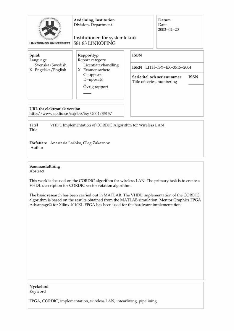
SammanfattningAbstract
This work is focused on the CORDIC algorithm for wireless LAN. The primary task is to create aVHDL description for CORDIC vector rotation algorithm.
The basic research has been carried out in MATLAB. The VHDL implementation of the CORDICalgorithm is based on the results obtained from the MATLAB simulation. Mentor Graphics FPGAAdvantage© for Xilinx 4010XL FPGA has been used for the hardware implementation.
NyckelordKeyword
FPGA, CORDIC, implementation, wireless LAN, intearliving, pipelining


Abstract
This work is focused on the CORDIC algorithm for wireless
LAN. The primary task is to create a VHDL description for
CORDIC vector rotation algorithm.
The basic research has been carried out in MATLAB. The
VHDL implementation of the CORDIC algorithm is based
on the results obtained from the MATLAB simulation.
Mentor Graphics FPGA Advantage© for Xilinx 4010XL
FPGA has been used for the hardware implementation.
− i −

− ii −
Acknowledgments
This thesis has been written in Electronics Systems division,
department of Electrical Engineering, Linköpings Universitet in the
contents of the international master program in SoCware − Integrated
Systems for Communication and Media.
We would like to give thanks to all ISY department staff,
especially, our supervisor Kent Palmkvist for his useful advices and
continuous attention to us.
We also thank all our neighbors, especially Deborah Capello for
her help during all the time we were writing our thesis.
Special thanks our friend Fedor Merkelov for giving many
advices in VHDL language and MATLAB.
− iii −

− iv −

Table of Contents
1 Introduction.........................................................................................1
1.1 About CORDIC..............................................................................1
1.2 Wireless LAN.................................................................................1
1.3 Background....................................................................................2
2 WLAN basics.......................................................................................3
2.1 Modulation.....................................................................................3
2.2 OFDM system model......................................................................4
2.3 Maximum likelihood synchronization.............................................6
2.3.1 Correlation properties of r(·)...................................................6
2.3.2 The likelihood function............................................................7
2.3.3 Simultaneous estimation..........................................................8
2.3.4 Synchronization.......................................................................9
2.4 Correcting sample frequency error................................................10
3 Algorithm...........................................................................................13
3.1 Modes of the CORDIC algorithm.................................................13
3.2 Arithmetics...................................................................................15
3.3 Another method to implement CORDIC algorithm.......................17
4 Solution..............................................................................................19
4.1 MATLAB program.......................................................................19
4.2 VHDL program............................................................................24
4.2.1 Interleaving...........................................................................25
Input control block .....................................................................27
Arithmetic blocks, CORDIC.......................................................28
Output control block...................................................................28
4.2.2 Pipelining..............................................................................29
Input control block......................................................................29
− v −

Arithmetic blocks.......................................................................30
Output control block...................................................................30
4.3 FPGA implementation..................................................................31
5 Conclusion..........................................................................................33
5.1 Future work..................................................................................33
References.............................................................................................35
Abbreviations........................................................................................37
Appendix A MATLAB program..........................................................39
Appendix B Wave diagrams................................................................41
− vi −
Index of figuresFigure 1. QAM constellation......................................................................................3
Figure 2. OFDM system model...................................................................................5
Figure 3. Structure of OFDM signal with cyclically extended frames.........................6
Figure 4. Block diagram of timing and frequency synchronization algorithms...........9
Figure 5. Signals that generate the estimates...............................................................9
Figure 6. Receiver structure for correcting sample frequency error...........................10
Figure 7. The rotation and vectoring modes of the CORDIC algorithm....................13
Figure 8. Block diagram of CORDIC algorithm.......................................................15
Figure 9. Calculations of vector angle.......................................................................20
Figure 10. Angle absolute values..............................................................................21
Figure 11. Accuracy calculation................................................................................22
Figure 12. Main block of VHDL program................................................................24
Figure 13. Structure diagram of interleaved VHDL block........................................25
Figure 14. Input control block..................................................................................27
Figure 15. CORDIC block........................................................................................28
Figure 16. Output control block................................................................................28
Figure 17. Structure diagram of pipelined VHDL architecture..................................29
Figure 18. Input control block..................................................................................29
Figure 19. Arithmetic blocks for pipelined version...................................................30
Figure 20. Output control block................................................................................30
Index of TablesTable 1. CORDIC accuracy and minimal number of steps........................................23
Table 2. Angle calculation........................................................................................26
Table 3. Signal structure...........................................................................................26
Table 4. FPGA utilization.........................................................................................31
− vii −

− viii −

1 Introduction 1
1 Introduction
1.1 About CORDICAll trigonometric functions can be computed using vector rotation. The
CORDIC (COordinate Rotation DIgital Computer) algorithm was developed by
Volder [6] in 1959. It rotates the vector, step−by−step, with a given angle.
Additional theoretical work has been done by Walther [7] in 1971. The main
principle of CORDIC are calculations based on shift−registers and adders
instead of multiplications, what saves much hardware resources.
CORDIC is used for polar to rectangular and rectangular to polar
conversions and also for calculation of trigonometric functions, vector
magnitude and in some transformations, like discrete Fourier transform (DFT)
or discrete cosine transform (DCT).
In particular case, the CORDIC algorithm is used in wireless LAN
(WLAN) by receivers.
1.2 Wireless LAN
Wireless LAN is specified with IEEE 802.11 standard. It was accepted in
1999 and led to organization of local networks development. WLAN is a
flexible data communications system implemented to extend or substitute for, a
wired LAN. Radio frequency (RF) technology is used by a wireless LAN to
transmit and receive data over the air, minimizing the need for wired
connections. A WLAN enables data connectivity and user mobility [8].

2 1 Introduction
1.3 Background
The main purpose of current work is to make the necessary research and
implement the CORDIC algorithm for wireless LAN. This algorithm calculates
the angle of a received vector in a signal constellation by means of the
arctangent function, and it is used in receivers to find frequency offset and phase
shift.
The work is targeted to research the number of bits of the input vector and
angle signals and specify the number of steps for a recursive CORDIC
algorithm. The research and intermediate results are made in the MATLAB 6.5
environment, and the final program has been implemented in the VHDL
language for FPGA.

2 WLAN basics 3
2 WLAN basics
This chapter describes the basic theoretical aspects, regarded to current
work, which show how the angle calculation is used by a receiver.
2.1 Modulation
Modulation is the process of transforming the carrier into waveforms
suitable for transmission across channel, according to parameters of modulated
signal [2].
The most useful type of modulation for OFDM (orthogonal frequency
division multiplexing) is quadrature amplitude modulation (QAM). It is shown
on Figure 1. QAM changes phase and amplitude of the carrier, and it is a
combination of amplitude shift keying (ASK) and phase shift keying (PSK).
Figure 1. QAM constellation
2
4
6
2 4 6−2−4−6
−2
−4
−6
QPSK
16−QAM
64−QAM
I
Q

4 2 WLAN basics
Equation 1 shows how amplitude and phase are combined in QAM, represented
in so−called IQ−form [1]:
s t =I k cos ωc t BQk sin ωc t =Ak cos ωc t+φk , (1)where
Ak= I k2+Qk
2 − amplitude,
φk=tanB1 Qk
I k
− phase.
In this work 64−QAM has been used.
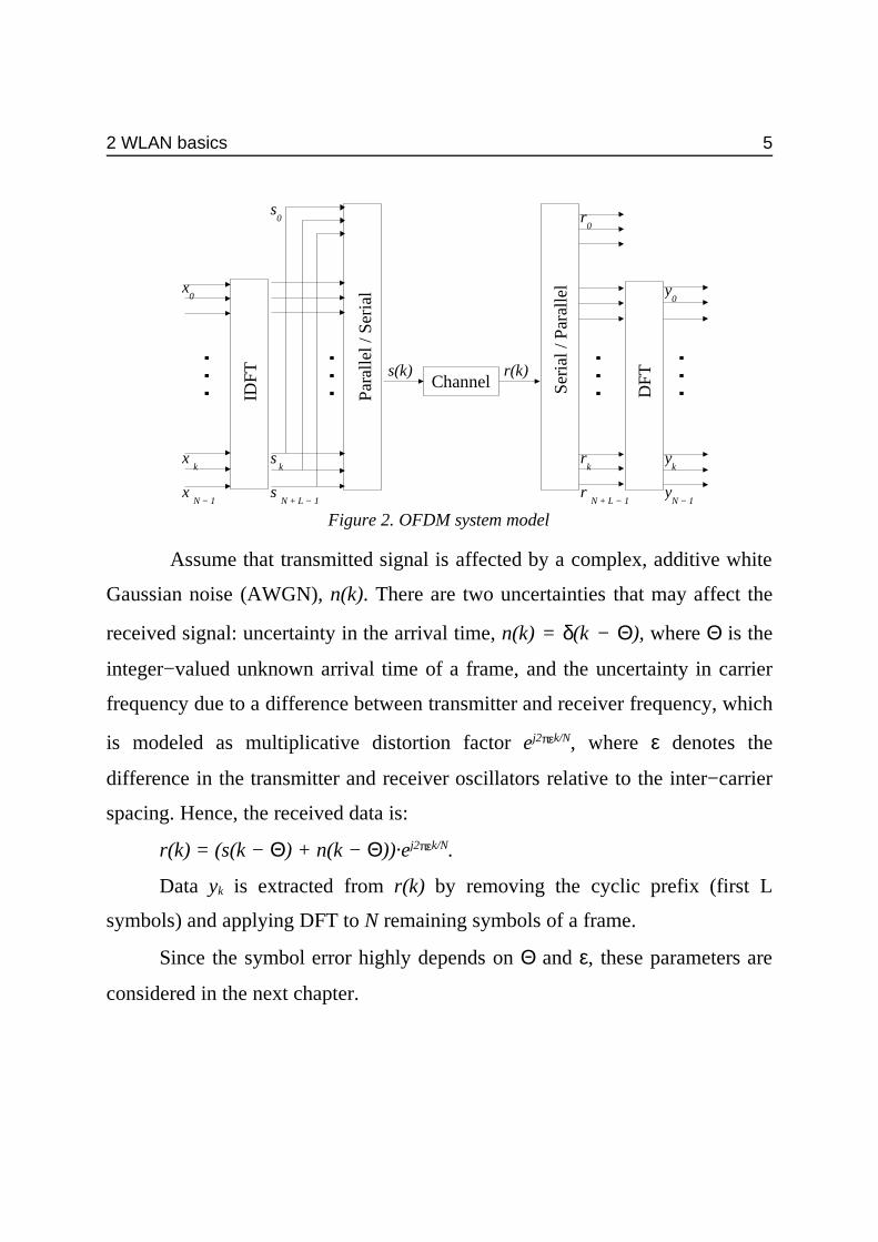
2.2 OFDM system modelConsider the transmission of a signal through a wireless channel.
Assume that OFDM modulation is used. It could be amplitude modulation as
well as PSK. The signal in a channel is normally represented as a sequence of
complex numbers, xk, from the signal constellation, which is modulated with N
subcarriers by an inverse DFT. It is divided in frames. Each OFDM frame
consist of N+L samples (see Figure 2), where last L samples are copy of first L
samples (cyclic prefix). The transmission is performed over a discrete−time
channel [3].
2 WLAN basics 5
Figure 2. OFDM system model
Assume that transmitted signal is affected by a complex, additive white
Gaussian noise (AWGN), n(k). There are two uncertainties that may affect the
received signal: uncertainty in the arrival time, n(k) = δ(k − Θ), where Θ is the
integer−valued unknown arrival time of a frame, and the uncertainty in carrier
frequency due to a difference between transmitter and receiver frequency, which
is modeled as multiplicative distortion factor ej2πεk/N, where ε denotes the
difference in the transmitter and receiver oscillators relative to the inter−carrier
spacing. Hence, the received data is:
r(k) = (s(k − Θ) + n(k − Θ))·ej2πεk/N.
Data yk is extracted from r(k) by removing the cyclic prefix (first L
symbols) and applying DFT to N remaining symbols of a frame.
Since the symbol error highly depends on Θ and ε, these parameters are
considered in the next chapter.
Channel
IDF
T
DF
T
Ser
ial /
Par
alle
l
Par
alle
l / S
eria
lx0
x N − 1
x k
s0
s k
s N + L − 1
s(k) r(k)
r0
rk
r N + L − 1
y0
yk
yN − 1
. . .
. . .
. . .
. . .
6 2 WLAN basics
2.3 Maximum likelihood synchronization
This paragraph illustrates the main theoretical aspects regarded to the
synchronization in WLANs. More formally this material is shown in [3].
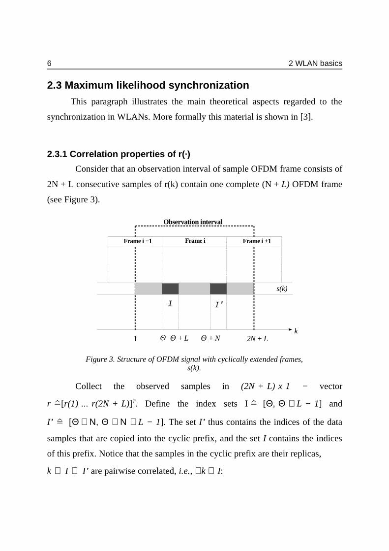
2.3.1 Correlation properties of r(·)
Consider that an observation interval of sample OFDM frame consists of
2N + L consecutive samples of r(k) contain one complete (N + L) OFDM frame
(see Figure 3).
Collect the observed samples in (2N + L) x 1 − vector
r «�[r(1) ... r(2N + L)]T. Define the index sets I « [Θ, Θ + L − 1] and
I’ « [Θ + Ν, Θ + Ν + L − 1]. The set I’ thus contains the indices of the data
samples that are copied into the cyclic prefix, and the set I contains the indices
of this prefix. Notice that the samples in the cyclic prefix are their replicas,
k ∈ I ∪ I’ are pairwise correlated, i.e., ∀k ∈ I:
Figure 3. Structure of OFDM signal with cyclically extended frames,s(k).
I I'
k2N + L
s(k)
1 Θ
Frame i
Observation interval
Frame i −1 Frame i +1
Θ + L Θ + N

2 WLAN basics 7
E r k r k+m =σ s
2+σn2 m=0
σ s2⋅eℑ2 ρε m=N
0 othervise
where σ s2«E s k 2 and σn
2«E n k 2 , while the remaining samples
k ∉ Ι ∪ Ι’ are mutually uncorrelated.
2.3.2 The likelihood function
The log−likelihood function for Θ and ε is the logarithm of the
probability density function of observing the 2N + L samples in r given the
arrival time Θ and the carrier frequency offset ε:
Λ Θ ,ε =log f r|Θ ,ε . (2)
The ML (maximum likelihood) estimate Θ̂ , ε̂ is the maximizing
argument of this function. If the condition (Θ, ε) is dropped for notational
clarity, (2) can be written as:Λ Θ ,ε =
= log ∏k∈I
f r k ,r k+N ∏k∉I ∪I’
f r k =
= log ∏k∈I
f r k ,r k+N
f r k f r k+N∏
k
f r k
(3)
where f(·) denotes the probability density function of its respective arguments.
The last factor in (3) is independent of Θ and may be dropped. Then, (3)
becomes:
Λ Θ ,ε = ∑k=Θ
Θ+LB1
2 ℜ e j2Πε r k r∗ k+N Bρ r k 2+ r k+N 2 , (4)
where ρ«σ s
2
σ s2+σn
2 is the magnitude of the correlation coefficient between
r(k) and r(k + N).
,

8 2 WLAN basics
2.3.3 Simultaneous estimation
The maximization of the log−likelihood function, can be performed in
two steps:
maxΘ ,ε
Λ Θ ,ε =maxΘ
maxε
Λ Θ ,ε =maxΘ
Λ Θ , ε̂ Θ
To find the maximum with respect to the frequency offset ε, we set the
derivate of the log−likelihood function (4) to zero and obtain
tan ε̂ Θ =B
ℑ ∑k=Θ
Θ+LB1
r k r∗ k+N
ℜ ∑k=Θ
Θ+LB1
r k r∗ k+N
.
By substitution of the ML−estimate ε̂ Θ the log−likelihood function
for Θ ,Λ Θ , ε̂ Θ can be calculated, and the maximum with respect to Θ can
be found. The simultaneous ML−estimation of Θ and ε becomes:
Θ̂=arg maxΘ
λ Θ , ε̂=B 1
2πγ Θ |Θ=Θ̂ ’ (5)
where
λ Θ =2 ∑k=Θ
Θ+LB1
r k r∗ k+N Bρ ∑k=Θ
Θ+LB1
r k 2+ r k+N 2 ,
γ Θ =r ∑k=Θ
Θ+LB1
r k r∗ k+N .

2 WLAN basics 9
2.3.4 Synchronization.
A synchronizing algorithm based on the estimators in (5) can now be
designed. Figure 4 shows the estimators in a block diagram. Figure 5 shows two
essential signals that are generated if a received signal consisting of several
OFDM frames is processed continuously by this estimator.
Figure 4. Block diagram of timing and frequency synchronization algorithms
ρ•2
ρ•2
zN
(•)∗
2•
r B 1
2π
⊕ ⊕
⊗
movingsum
movingsum
argmax
r(k)
−
+
λ(θ)
γ(θ) ε̂
Θ̂
Figure 5. Signals that generate the estimates
10 2 WLAN basics
The estimation methods can be improved if the parameters Θ and ε can
be considered constant over several OFDM frames. If the observation interval
contains M completed OFDM frames the log−likelihood function of Θ and ε
given this observation interval becomes
Λ Θ ,ε = 1
M∑m=0
M B1
Λm Θ ,ε ,
where Λm Θ ,ε is the log−likelihood function of Θ and ε given that
only frame m is observed. Thus, to obtain the log−likelihood function, the log−
likelihood functions of the individual frames must be averaged.
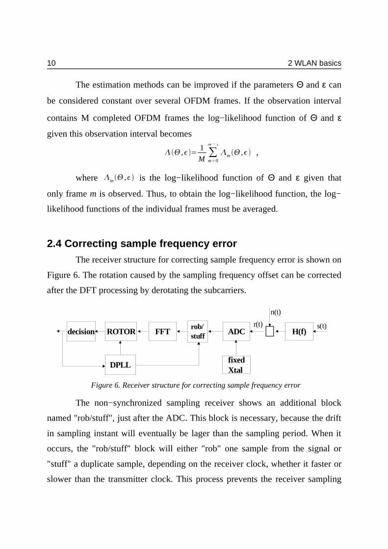
2.4 Correcting sample frequency errorThe receiver structure for correcting sample frequency error is shown on
Figure 6. The rotation caused by the sampling frequency offset can be corrected
after the DFT processing by derotating the subcarriers.
Figure 6. Receiver structure for correcting sample frequency error
The non−synchronized sampling receiver shows an additional block
named "rob/stuff", just after the ADC. This block is necessary, because the drift
in sampling instant will eventually be lager than the sampling period. When it
occurs, the "rob/stuff" block will either "rob" one sample from the signal or
"stuff" a duplicate sample, depending on the receiver clock, whether it faster or
slower than the transmitter clock. This process prevents the receiver sampling
decision H(f)
fixedXtal
ROTOR FFT ADCrob/stuff
DPLL
⊕r(t)
n(t)
s(t)

2 WLAN basics 11
instant from drifting so much that the symbol timing would be incorrect. The
"ROTOR" block performs the required phase corrections with the information
provided by the Digital Phase−Locked Loop (DPLL) that estimates the sampling
frequency error [2].

12

3 Algorithm 13
3 Algorithm
CORDIC is based on the common rotation equations:x’=x⋅cosφBy⋅sinφ=cosφ⋅ xBy⋅tanφy’=y⋅cosφ+x⋅sinφ=cosφ⋅ y+x⋅tanφ
(6)
If tan φ = ±2−i, multiplication in (6) can be performed by a simple shift
operation. This allows the vector to be rotated by desired angle in a sequence of
smaller rotations by angle φι = ± tan−1 (2−i):
xi+1 = ki [xi − yi · di · 2−i]
yi+1 = ki [yi + xi · di · 2−i],
where k i=cos tanB1 2Bi =1 ⁄ 1+2B2i , d i=±1 .
3.1 Modes of the CORDIC algorithm
CORDIC rotator works in two modes: rotation and vectoring (Figure 7)
[5].
Figure 7. The rotation (X’, Y’) and vectoring(X, Y) modes of the CORDIC algorithm
Y’
Y
R
X’ X
θα

14 3 Algorithm
In the first mode it rotates the input vector by specified angle. The angle
accumulator is initialized with the desired rotation angle. For this mode,
CORDIC equations are:
xi+1 = xi − yi * di* 2−i
yi+1 = yi + xi * di* 2−i
zi+1 = zi − di * tan−1( 2−i),
where d i=B1, z i<0
1, otherwise
This gives the following result:
xn = An· [x0 cosz0 − y0 sinz0]
yn = An· [y0 cosz0 − x0 sinz0]
zn = 0,
where An = ∏n
1+2B2i
.
In the vectoring mode input vector is being rotated to the x axis while
recording the angle required to make that rotation. The result of the vectoring
operation is a rotation angle and the scaled magnitude of original vector. The
CORDIC equations in this mode are:
xi+1 = xi − yi * di* 2−i
yi+1 = yi + xi * di* 2−i
zi+1 = zi − di * tan−1( 2−i),
where d i=B1, y i<0
1, otherwise(7)
Then:
xn = An20
20 yx +
yn = 0

3 Algorithm 15
zn = z0 + tan−1 (0
0x
y)
An = ∏ −+n
i221
The CORDIC algorithm in every mode is limited between 2
π− and 2π .
This limitation is caused by the first rotation angle φ0 = tan−1(20).
3.2 ArithmeticsFigure 8 represents the block diagram of conventional CORDIC
algorithm [10], based on ripple carry adders or subtractors.
Figure 8. Block diagram of CORDIC algorithm
A/S
±
A/S
±
A/S
±
A/S
±
A/S
±
A/S
±
X0
Y0
Xn
Yn
σ̄0
σ̄1
σ̄nB1
σ0
σ1
σnB1
X1 Y1X
12B1
Y1 2B1
XnB1
2n+1YnB1
2n+1XnB1
YnB1
16 3 Algorithm
An adder/subtractor (A/S), depending on a selection input, performs an
addition or a subtraction. This input indicates whether an operand is negative.
The basic cell of A/S is decomposed by two functions with 4 bits input each.
One of them is for calculating the output and another to transmit the carry.
According to this an N−bit A/S can fit in (2N+1)/2 CLBs (configurable logic
block). The additional half CLB is required for introducing the least significant
bit (LSB) one in case of the substraction. The critical path here is indicated by
the ripple carry propagation and the routing delay of the A/S wire. This net has a
fan−out of 2N in this case. It decreases the performance of the circuit and it is
the main disadvantage of conventional CORDIC implementations. As the
solution to this, redundant arithmetic could be used to increase the speed of the
CORDIC. Implementation avoids the carry propagation from the LSB to the
most significant bit (MSB), due to its carry−free property.
Redundant arithmetic is good to accelerate those operations, which have
a long propagation delay. On the other hand redundant arithmetic also has some
disadvantages. For example, it is impossible to detect the sign of a redundant
number without checking all the digits which expects a propagation from the
MSB to the LSB. Another problem, that the redundant arithmetic uses digit set
{−1,0,1}, and needs more hardware resources to execute simple tasks, than the
conventional one which uses digit set {−1,1}.
According to results of the research, the redundant arithmetic is more
accurate, but it needs much more hardware than the conventional arithmetic and
for this reason conventional arithmetic has been used in this work.
3 Algorithm 17
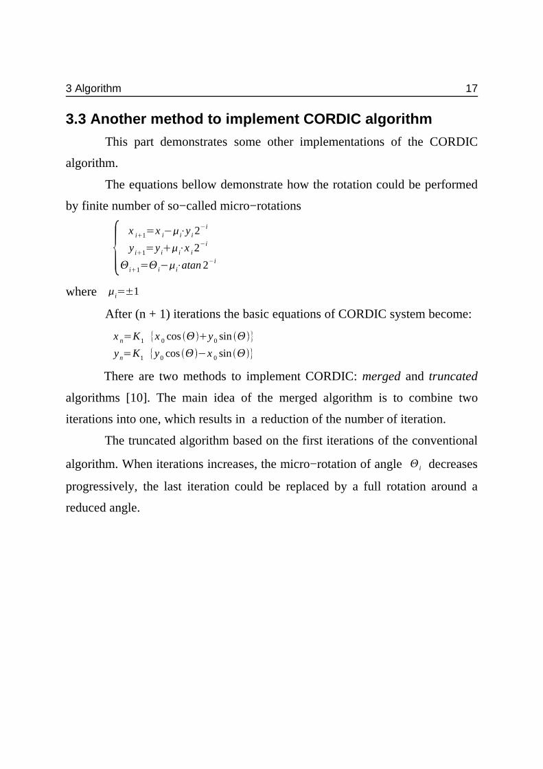
3.3 Another method to implement CORDIC algorithm
This part demonstrates some other implementations of the CORDIC
algorithm.
The equations bellow demonstrate how the rotation could be performed
by finite number of so−called micro−rotations
x i+1=x iBµi⋅y i 2Bi
y i+1=y i+µi⋅x i 2Bi
Θi+1=ΘiBµi⋅atan 2Bi
where µi=±1
After (n + 1) iterations the basic equations of CORDIC system become:
x n=K1 x 0 cos Θ +y0 sin Θ
yn=K1 y0 cos Θ Bx 0 sin Θ
There are two methods to implement CORDIC: merged and truncated
algorithms [10]. The main idea of the merged algorithm is to combine two
iterations into one, which results in a reduction of the number of iteration.
The truncated algorithm based on the first iterations of the conventional
algorithm. When iterations increases, the micro−rotation of angle Θi decreases
progressively, the last iteration could be replaced by a full rotation around a
reduced angle.

18

4 Solution 19
4 SolutionThe work has been started with the research in MATLAB. There are two
versions of VHDL program, based on MATLAB research.
4.1 MATLAB programIt is good approach to start to research the CORDIC algorithm in the
MATLAB environment.
MATLAB has been chosen for this purpose because:
: It provides very good arithmetic methods, functions, and graphical interface,
that will decrease the time of programming.
: The MATLAB language allows to create both small draft applications and
big complicated programs.
: Models are easy to debug.
It works in many different operating systems as Windows, UNIX
(Solaris) and Mac OS.
The main use of the MATLAB program is to debug the CORDIC
algorithm and to understand how accurate the angle value should be.
20 4 Solution
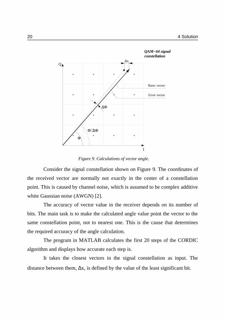
Consider the signal constellation shown on Figure 9. The coordinates of
the received vector are normally not exactly in the center of a constellation
point. This is caused by channel noise, which is assumed to be complex additive
white Gaussian noise (AWGN) [2].
The accuracy of vector value in the receiver depends on its number of
bits. The main task is to make the calculated angle value point the vector to the
same constellation point, not to nearest one. This is the cause that determines
the required accuracy of the angle calculation.
The program in MATLAB calculates the first 20 steps of the CORDIC
algorithm and displays how accurate each step is.
It takes the closest vectors in the signal constellation as input. The
distance between them, ∆x, is defined by the value of the least significant bit.
Figure 9. Calculations of vector angle.
Basic vector
Error vector
QAM−64 signalconstellation
Φ
Φ+∆Φ
∆Φ
∆x
I
Q

4 Solution 21
For example, if it equals to 2−2, then the distance between these two
vectors is 0.25, and the accuracy, ∆Φ, should be less than 0.02.
The program looks onto the CORDIC arctangent values on each step,
and interpolates them to an exponent using a built−in MATLAB function. Then,
depending on this interpolation and inaccuracy values, it finds the minimal
number of steps necessary to calculate the angle.
The text of program is given in Appendix A.
As a result, program plots two graphics: the angle values at each step,
and the accuracy of those values, as is shown on Figures 10 and 11.
Figure 10. Angle absolute values

22 4 Solution
Figure 11 shows CORDIC algorithm calculated in 2 ways:
� when factor d in (7) belongs to conventional arithmetic, i.e., d ∈ (−1; 1);
� when d belongs to set (−1; 0; 1) from the redundant arithmetic.
As it can be seen from this Figure, the redundant arithmetic does not
have much gain against conventional arithmetic, but it takes more hardware
resources to decide whether to perform rotation on each step or not. Hence the
redundant arithmetic is not a good approach, and for this reason the
conventional one is selected to write the program.
This program has been used to research accuracy and minimal number
of CORDIC steps. From geometry point of view, input vectors must be
maximally remote from the center of signal constellation to obtain maximum
Figure 11. Accuracy calculation

4 Solution 23
accuracy value. This gives minimal value of ∆Φ (see Figure 9). The result is
shown in Table 1.
Table 1. CORDIC accuracy and minimal number of steps
Vectorwidth*, (bit) Range* Vector accuracy Angle accuracy, (rad) Nmin
4 [−8; 7] 20 = 1 0.07677189 ≥ 2−4 5
5 [−8; 7.5] 2−1 = 0,5 0.03934975 ≥ 2−5 6
6 [−8; 7.75] 2−2 = 0,25 0.01985645 ≥ 2−6 7
7 [−8; 7.875] 2−3 = 0.125 0.00996644 ≥ 2−7 8
8 [−8; 7.9375] 2−4 = 0.0625 0.00499195 ≥ 2−8 9
9 [−8; 7.96875] 2−5 = 0.03125 0.00249801 ≥ 2−9 10
10 [−8; 7.984375] 2−6 = 0.015625 0.00124951 ≥ 2−10 11
11 [−8; 7.9921875] 2−7 = 0.0078125 0.00062488 ≥ 2−11 12
12 [−8; 7.99609375] 2−8 = 0.00390625 0.00031247 ≥ 2−12 13*effective width, same for real and imaginary parts
According to a given specification the input vector has 12 bit length and
therefore its accuracy is 2−8. Hence, the angle accuracy is 2−12 and the number of
steps required for calculations is 13. Due to the probability theory, the received
vector is normally close to the center of constellation point and not close to a
boundary between points. This means that so high accuracy is not actually
needed for calculations and the number of steps can be reduced.
From the theoretical point of view, IEEE 802.11a standard has data bit
rate of 20MSamples/s and FPGA has the clock frequency of 100 MHz that gives
the sample periods of 5 clock cycles. Then, the effective number of steps must
be 5·k, where k has a natural value.
From research in MATLAB it has been found that 5 CORDIC steps are
not enough to obtain accurate results, but 10 steps give higher accuracy. Even
higher accuracy could be given by 15 CORDIC steps, but it is actually not
proved. Hence, the number of steps required to get the necessary angle accuracy
should be equal to 10. This allows for an input vector of 9 bit for both real and

24 4 Solution
imaginary parts and output 12 bits (3 bit per integer part and 9 bits per fractional
part).
There is also a tradeoff to specify bit width for the internal vector signals
because the vectoring mode CORDIC angle rotation uses the sign of the
imaginary part to specify the direction of the rotation, and it must be correct in
all steps. Since the imaginary part gets closer and closer to ’0’, it must have
enough round bits. The practical tests in the VHDL testbench show that 15 to 16
bits are enough.
4.2 VHDL program
There are two realizations of the VHDL program in Mentor Graphics
FPGA Advantage© tool for Xilinx 4010XL FPGA. Since the found number of
steps in MATLAB is equal to 10, one VHDL program uses interleaving of
processing blocks and other uses pipelining.
The main block is the same for both programs, and it is shown on Figure
12. It inputs a complex vector. The signal start indicates that values on input are
ready, and the program should output angle value.
This block consists of two control units and two arithmetic blocks.
Figure 12. Main block of VHDL program.
clk
rst
start
in_real
in_img
angleCORDICmain
4 Solution 25
Consider each program separately.
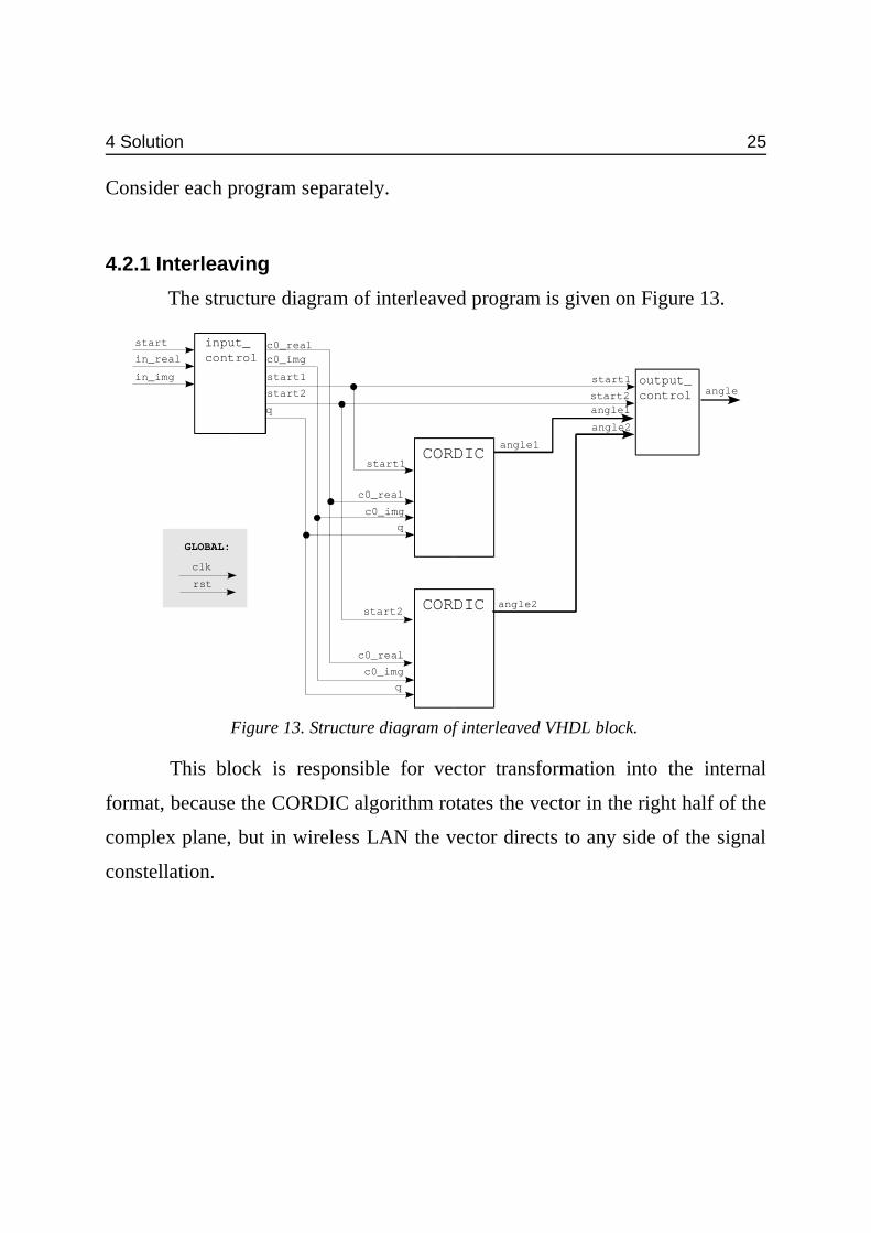
4.2.1 Interleaving
The structure diagram of interleaved program is given on Figure 13.
This block is responsible for vector transformation into the internal
format, because the CORDIC algorithm rotates the vector in the right half of the
complex plane, but in wireless LAN the vector directs to any side of the signal
constellation.
Figure 13. Structure diagram of interleaved VHDL block.
start1
start2
start
clk
rst
angle1
angle2
angle
input_control
output_control
CORDIC
CORDIC
c0_imgc0_real
start1
start2angle1
angle2
in_real
in_img
GLOBAL:
q
start1
start2
q
q
c0_img
c0_img
c0_real
c0_real
26 4 Solution
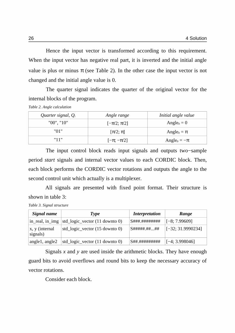
Hence the input vector is transformed according to this requirement.
When the input vector has negative real part, it is inverted and the initial angle
value is plus or minus π (see Table 2). In the other case the input vector is not
changed and the initial angle value is 0.
The quarter signal indicates the quarter of the original vector for the
internal blocks of the program.
Table 2. Angle calculation
Quarter signal, Qi Angle range Initial angle value
"00", "10" [−π/2; π/2] Angle0 = 0
"01" [π/2; π] Angle0 = π
"11" [−π; −π/2] Angle0 = −π
The input control block reads input signals and outputs two−sample
period start signals and internal vector values to each CORDIC block. Then,
each block performs the CORDIC vector rotations and outputs the angle to the
second control unit which actually is a multiplexer.
All signals are presented with fixed point format. Their structure is
shown in table 3:
Table 3. Signal structure
Signal name Type Interpretation Range
in_real, in_img std_logic_vector (11 downto 0) S###.######## [−8; 7.99609]
x, y (internalsignals)
std_logic_vector (15 downto 0) S#####.##...## [−32; 31.9990234]
angle1, angle2 std_logic_vector (11 downto 0) S##.######### [−4; 3.998046]
Signals x and y are used inside the arithmetic blocks. They have enough
guard bits to avoid overflows and round bits to keep the necessary accuracy of
vector rotations.
Consider each block.
4 Solution 27
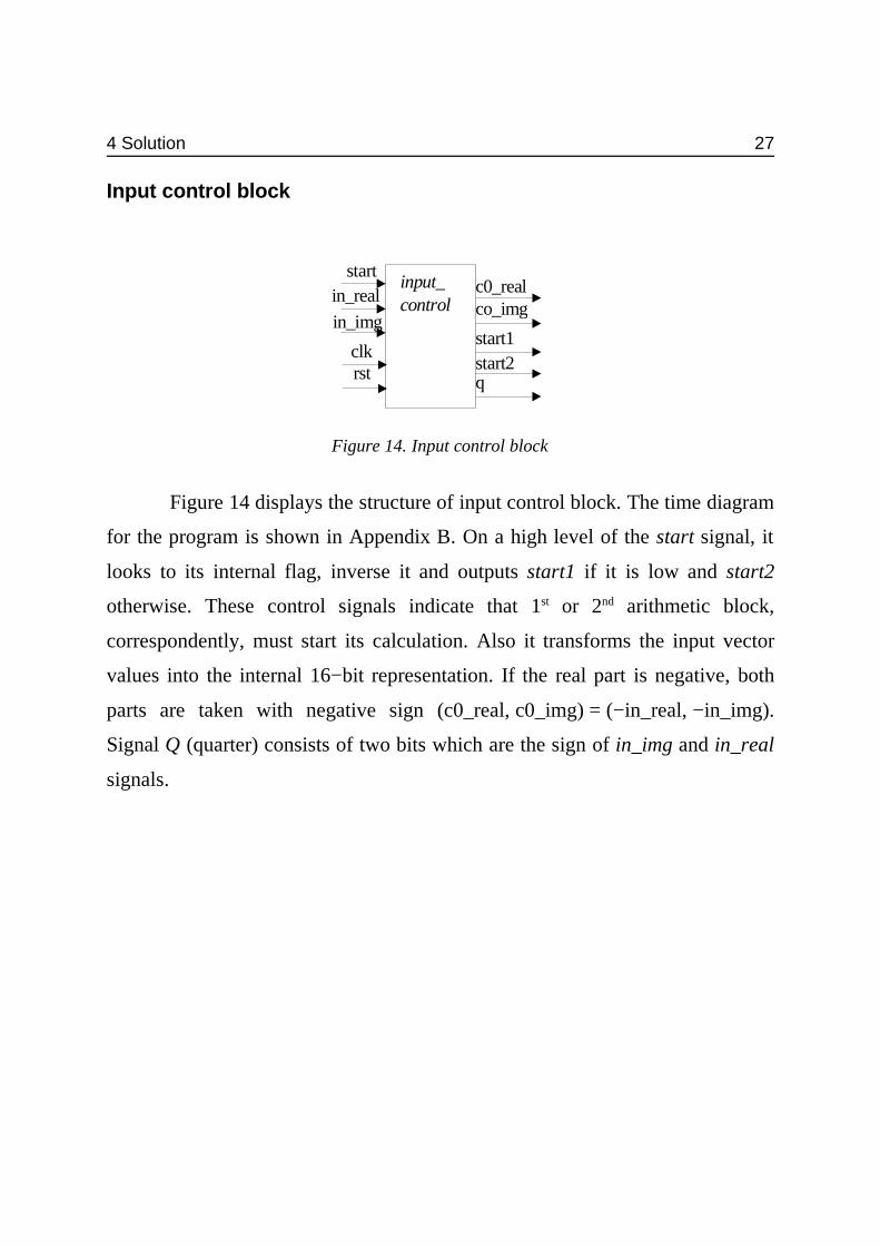
Input control block
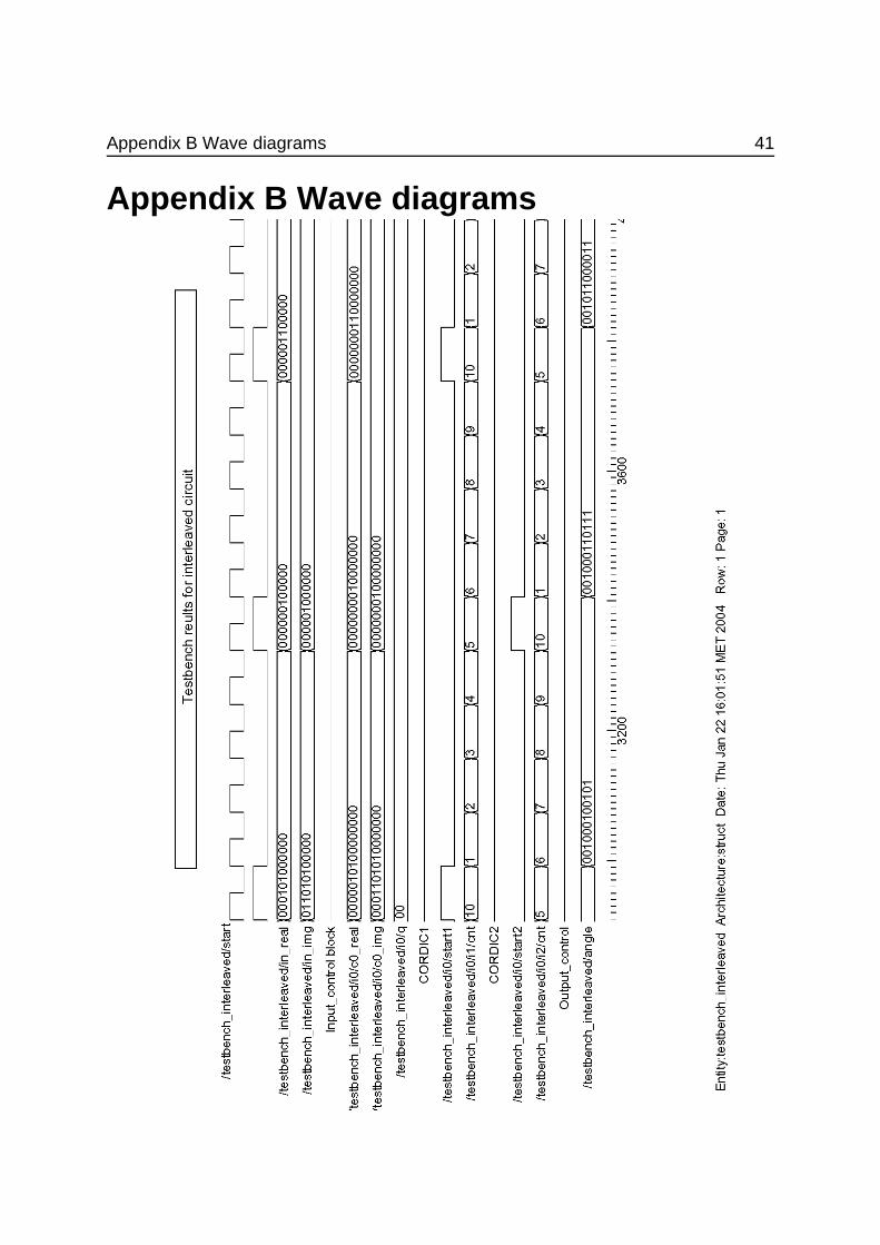
Figure 14 displays the structure of input control block. The time diagram
for the program is shown in Appendix B. On a high level of the start signal, it
looks to its internal flag, inverse it and outputs start1 if it is low and start2
otherwise. These control signals indicate that 1st or 2nd arithmetic block,
correspondently, must start its calculation. Also it transforms the input vector
values into the internal 16−bit representation. If the real part is negative, both
parts are taken with negative sign (c0_real, c0_img) = (−in_real, −in_img).
Signal Q (quarter) consists of two bits which are the sign of in_img and in_real
signals.
Figure 14. Input control block
input_control
clkrst
start
start1start2
in_real
in_img
c0_realco_img
q
28 4 Solution
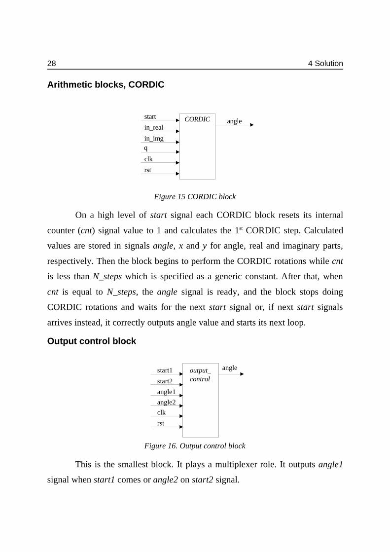
Arithmetic blocks, CORDIC
On a high level of start signal each CORDIC block resets its internal
counter (cnt) signal value to 1 and calculates the 1st CORDIC step. Calculated
values are stored in signals angle, x and y for angle, real and imaginary parts,
respectively. Then the block begins to perform the CORDIC rotations while cnt
is less than N_steps which is specified as a generic constant. After that, when
cnt is equal to N_steps, the angle signal is ready, and the block stops doing
CORDIC rotations and waits for the next start signal or, if next start signals
arrives instead, it correctly outputs angle value and starts its next loop.
Output control block
This is the smallest block. It plays a multiplexer role. It outputs angle1
signal when start1 comes or angle2 on start2 signal.
Figure 15 CORDIC block
CORDIC
clk
rst
startangle
in_real
in_imgq
Figure 16. Output control block
output_control
clk
rst
start1 angle
start2
angle1
angle2

4 Solution 29
4.2.2 Pipelining
This program is similar to program described above, but it divides the
CORDIC block into two parts, CORDIC1 and CORDIC2, with 5−clock cycle
per sample period each. The structural diagram is shown on Figure 17.
Input control block
This block is similar to input control block for interleaving version. It
transforms in_real and in_img signals into the internal format and outputs the q
signal in the same way. It also outputs pipelined start1 signal for all blocks
which indicates that a new sample period has begun.
Figure 17. Structure diagram of pipelined VHDL architecture
in_real
in_img
start
c0_real
c0_img
q : (1:0)
start1start1
start1
c1_real
c1_img
angle1
angle_in angle
output_control
CORDIC2CORDIC1input_control
clk
rst
GLOBAL:
Figure 18. Input control block.
in_real
in_imgstart
input_control
clkrst
c0_real
c0_img
q : (1:0)
start1
30 4 Solution
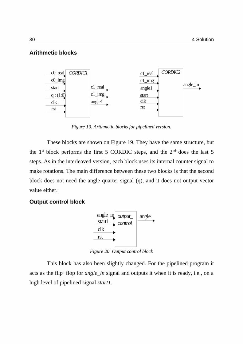
Arithmetic blocks
These blocks are shown on Figure 19. They have the same structure, but
the 1st block performs the first 5 CORDIC steps, and the 2nd does the last 5
steps. As in the interleaved version, each block uses its internal counter signal to
make rotations. The main difference between these two blocks is that the second
block does not need the angle quarter signal (q), and it does not output vector
value either.
Output control block
This block has also been slightly changed. For the pipelined program it
acts as the flip−flop for angle_in signal and outputs it when it is ready, i.e., on a
high level of pipelined signal start1.
Figure 19. Arithmetic blocks for pipelined version.
clkrst
clkrst
c0_real
c0_img
start
q : (1:0) start
c1_real
c1_img
angle1
CORDIC2CORDIC1
c1_real
c1_img
angle1
angle_in
Figure 20. Output control block
start1angle_in angleoutput_
controlclkrst

4 Solution 31
4.3 FPGA implementation
Both programs have been implemented in Leonardo tool for FPGA
4010xLPC84. Table 4 demonstrates that they have used about 50% of available
resources.
Table 4. FPGA utilization
Resource Interleaving Pipelining
Used Available Utilization Used Available Utilization
IOs 39 61 63.93% 39 61 63.93%
FG FunctionGenerators
447 800 55.88% 407 800 50.50%
H FunctionGenerators
198 400 49.50% 143 400 35.75%
CLB flip−flops 140 800 17.50% 136 800 17.12%
Theoretically interleaving of two blocks requires almost twice more area
than pipelining. This is proved by Table 4 despite of optimization of all blocks.
Hence, the pipelining is more preferable than interleaving, but if the arithmetic
block is complex and cannot be split into smaller blocks, the interleaving is the
only way to solve the task with all timing constraints.

32

5 Conclusion 33
5 Conclusion
In this work regarded to CORDIC implementation in VHDL there has
been done a specific research on angle calculation in wireless LAN receiver
block. As a result of this research there has been found vector and angle widths
necessary and sufficient for an implementation and the number of CORDIC
steps for calculating an arctangent function.
Then two programs have been written on VHDL language: one for an
interleaving and the other for a pipelining realizations, and there is found that a
pipelining implementation is better than an interleaving because it saves
hardware. Both programs have been implemented for FPGA 4010xLPC84 for
further implementation.
5.1 Future workDuring this work the program was implemented for the existing version
of FPGA with clock frequency of 12MHz that does not give the required sample
rate of 20 MSamples/sec. Therefore this program must be implemented to a new
version of FPGA with 100 MHz clock cycle to obtain the necessary sample rate.

34
References 35
References
[1] Nee R., Prasad R.: "OFDM for Wireless Multimedia Communications",
Boston: Artech House, 2000.
[2] Terry J., Heiskala J.: "OFDM Wireless LANs: A Theoretical and Practical
Guide", Indianapolis, Ind.: Sams, 2002.
[3] Sandell M., van de Beek J.−J., Börjesson P.: "Timing and Frequency
Synchronization in OFDM Systems Using the Cyclic Prefix", pp 16−19, Essen,
Germany, Desember 1995.
[4] Andraka R.: "A Survey of CORDIC Algorithms for FPGA Based
Computers", 1998
[5] Valls, J.; Kuhlmann, M.; Parhi, K.K.: "Efficient Mapping of CORDIC
Algorithms on FPGA", Signal Processing Systems, 2000. IEEE Workshop, pp
336−343 , 11−13 Oct. 2000.
[6] Volder J.E.: "The CORDIC Trigonometric Computing Technique", IRE
Trans. Electronic Computers, vol. EC−8, pp 330−334, 1959.
[7] Walter J.S. "A Unified Algorithm for Elementary Functions", Proc. Spring.
Joint Comput. Conference, vol. 38, pp 379−385, Jul. 1992.
[8] http://www.wirelesslan.tk/
[9] Hemkumar N.D.: "A Systolic VLSI Architecture for Complex SVD",
Houston, Texas, 1991.
[10] Kharrat, M.W.; Loulou, M.; Masmoudi, N.; Kamoun, L.: "A new method
to implement CORDIC algorithm", Electronics, Circuits and Systems, 2001.
ICECS 2001. The 8th IEEE International Conference on , vol 2, pp 715 − 718
Sept. 2001
[11] Armstrong, J.R., Gray F.G.: "VHDL Design Representation and Synthesis"
2nd edition, Upper Saddle River, N.J.: Prentice Hall PTR, 2000

36
Abbreviations 37
AbbreviationsADC − analog−digital convertor
A/S − adder/subtractor
ASK − amplitude shift keying
CORDIC − COordinate Rotation DIgital Computer
CLB − configurable logic block
DFT − discrete Fourier transform
DPLL − digital phase−locked loop
LSB − least significant bit
MSB − most significant bit
OFDM − orthogonal frequency−division multiplexing
QAM − quadrature amplitude modulation
PSK − phase shift keying
RF − radio frequency
VHDL − Very high speed integrated circuit Hardware Description Language
WLAN − Wireless Local Area Network

38
Appendix A MATLAB program 39
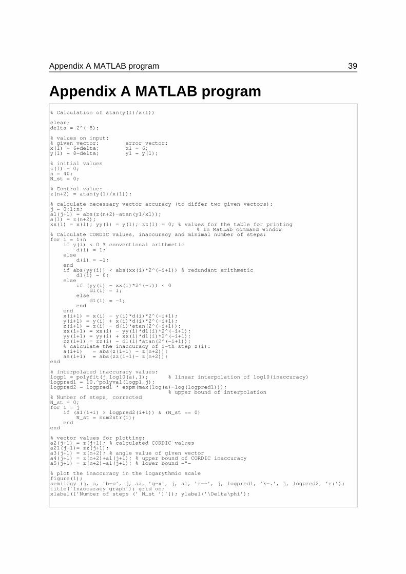
Appendix A MATLAB program% Calculation of atan(y(1)/x(1))
clear;delta = 2^(−8);
% values on input:% given vector: error vector:x(1) = 6+delta; x1 = 6;y(1) = 8−delta; y1 = y(1);
% initial valuesz(1) = 0;n = 40;N_st = 0;
% Control value:z(n+2) = atan(y(1)/x(1));
% calculate necessary vector accuracy (to differ two given vectors):j = 0:1:n;a1(j+1) = abs(z(n+2)−atan(y1/x1));a(1) = z(n+2);xx(1) = x(1); yy(1) = y(1); zz(1) = 0; % values for the table for printing
% in MatLab command window% Calculate CORDIC values, inaccuracy and minimal number of steps:for i = 1:n if y(i) < 0 % conventional arithmetic d(i) = 1; else d(i) = −1; end if abs(yy(i)) < abs(xx(i)*2^(−i+1)) % redundant arithmetic d1(i) = 0; else if (yy(i) − xx(i)*2^(−i)) < 0 d1(i) = 1; else d1(i) = −1; end end x(i+1) = x(i) − y(i)*d(i)*2^(−i+1); y(i+1) = y(i) + x(i)*d(i)*2^(−i+1); z(i+1) = z(i) − d(i)*atan(2^(−i+1)); xx(i+1) = xx(i) − yy(i)*d1(i)*2^(−i+1); yy(i+1) = yy(i) + xx(i)*d1(i)*2^(−i+1); zz(i+1) = zz(i) − d1(i)*atan(2^(−i+1)); % calculate the inaccuracy of i−th step z(i): a(i+1) = abs(z(i+1) − z(n+2)); aa(i+1) = abs(zz(i+1)− z(n+2));end
% interpolated inaccuracy values:logp1 = polyfit(j,log10(a),1); % linear interpolation of log10(inaccuracy)logpred1 = 10.^polyval(logp1,j);logpred2 = logpred1 * expm(max(log(a)−log(logpred1))); % upper bound of interpolation% Number of steps, correctedN_st = 0;for i = j if (a1(i+1) > logpred2(i+1)) & (N_st == 0) N_st = num2str(i); endend
% vector values for plotting:a2(j+1) = z(j+1); % calculated CORDIC valuesa21(j+1)= zz(j+1);a3(j+1) = z(n+2); % angle value of given vectora4(j+1) = z(n+2)+a1(j+1); % upper bound of CORDIC inaccuracya5(j+1) = z(n+2)−a1(j+1); % lower bound −"−
% plot the inaccuracy in the logarythmic scalefigure(1);semilogy (j, a, ’b−o’, j, aa, ’g−x’, j, a1, ’r−−’, j, logpred1, ’k−.’, j, logpred2, ’r:’);title(’Inaccuracy graph’); grid on;xlabel([’Number of steps (’ N_st ’)’]); ylabel(’\Delta\phi’);

40 Appendix A MATLAB program
% plot the CORDIC angle valuesfigure(2); plot(j, a2, ’b−’, j, a21, ’g−’, j, a3, ’g−.’, j, a4, ’r:’, j, a5, ’r:’);title(’Arctangent calculations’); grid on;xlabel([’Number of steps (’ N_st ’)’]); ylabel(’\phi’);
Appendix B Wave diagrams 41
Appendix B Wave diagrams

42
På svenska
Detta dokument hålls tillgängligt på Internet – eller dess framtida ersättare –under en längre tid från publiceringsdatum under förutsättning att inga extra−ordinära omständigheter uppstår.
Tillgång till dokumentet innebär tillstånd för var och en att läsa, ladda ner,skriva ut enstaka kopior för enskilt bruk och att använda det oförändrat förickekommersiell forskning och för undervisning. Överföring av upphovsrättenvid en senare tidpunkt kan inte upphäva detta tillstånd. All annan användning avdokumentet kräver upphovsmannens medgivande. För att garantera äktheten,säkerheten och tillgängligheten finns det lösningar av teknisk och administrativart.
Upphovsmannens ideella rätt innefattar rätt att bli nämnd som upphovsman iden omfattning som god sed kräver vid användning av dokumentet på ovanbeskrivna sätt samt skydd mot att dokumentet ändras eller presenteras i sådanform eller i sådant sammanhang som är kränkande för upphovsmannens litteräraeller konstnärliga anseende eller egenart.
För ytterligare information om Linköping University Electronic Press seförlagets hemsida http://www.ep.liu.se/
In English
The publishers will keep this document online on the Internet − or its possiblereplacement − for a considerable time from the date of publication barringexceptional circumstances.
The online availability of the document implies a permanent permission foranyone to read, to download, to print out single copies for your own use and touse it unchanged for any non−commercial research and educational purpose.Subsequent transfers of copyright cannot revoke this permission. All other usesof the document are conditional on the consent of the copyright owner. Thepublisher has taken technical and administrative measures to assure authenticity,security and accessibility.
According to intellectual property law the author has the right to bementioned when his/her work is accessed as described above and to be protectedagainst infringement.
For additional information about the Linköping University Electronic Pressand its procedures for publication and for assurance of document integrity,please refer to its WWW home page: http://www.ep.liu.se/
© Anastasia Lashko, Oleg Zakaznov