Vertical Integration and Firm Productivity

Hongyi LI Yi LU Zhigang TAO∗

This version: August 2016

Abstract

This paper uses three cross-industry datasets from China and other devel-

oping countries to study the effect of vertical integration on firm productivity.

Our findings suggest that vertical integration has a negative impact on pro-

ductivity, in contrast to recent studies based on U.S. firms. We argue that

in settings with poor corporate governance, vertical integration reduces firm

productivity because it enables inefficient rent-seeking by insiders.

Keywords: Vertical Integration; Firm Productivity; Rent-Seeking; Corporate

Governance; Panel Estimation

JEL Codes: L22, D23, L25

∗Li: UNSW, hongyi@unsw.edu.au. Lu: National University of Singapore, ecsluyi@nus.edu.sg.Tao: The University of Hong Kong, ztao@hku.hk. We thank the coeditor and two anonymous refereesfor their suggestions and criticisms; Oliver Hart for his comments on an earlier version of this paper;and Adam Solomon and Lianming Zhu for excellent research assistance.

1

1 Introduction

This paper examines the impact of vertical integration on firm productivity. To do

so, we analyze two different cross-industry datasets of Chinese manufacturing firms

and another dataset of firms in developing countries, drawn from various surveys

conducted between 1998 and 2006.

We find that firm productivity, as measured by labour productivity, decreases with

vertical integration in each of our datasets. Our results are in contrast to recent em-

pirical findings, largely based on U.S. data (e.g., Hortacsu and Syverson, 2007; Forbes

and Lederman, 2010) that vertical integration improves firm efficiency. We propose

a simple explanation for this negative relationship: in developing-country settings

characterized by poor legal protections for firms’ investors, vertical integration may

serve as an inefficient means for parties in control to extract private benefits.

A number of problems arise when estimating the causal impact of vertical in-

tegration. One concern is the endogeneity problem, whereby omitted-variable bias

arises because firms’ vertical integration decisions are nonrandom. In particular,

such nonrandomness may arise because firms condition their integration decisions

on unobserved factors. A special case of the endogeneity problem is what Gibbons

(2005) aptly labels the ‘Coase-meets-Heckman’ problem: if integration is compara-

tively advantageous at high-difficulty transactions (which are likely to produce inef-

ficient outcomes relative to the first-best), and if transaction difficulty is unobserved,

then simple correlations will naively produce a negative relationship between vertical

integration and firm productivity.

A second concern is the mismeasurement problem: the extent of vertical integra-

tion may be mismeasured in conventional (indirect) measures for vertical integration.

For example, the value-added ratio is used extensively in the literature as a measure

of vertical integration, but may be sensitive to the stage of the production process in

2

which a given firm specializes.1 Mismeasurement of vertical integration may lead to

estimation biases even when the integration decisions are randomly determined (i.e.,

even in the absence of endogeneity problems). For example, when both the integra-

tion decision and the mismeasurement of vertical integration are uncorrelated with

unobserved firm characteristics, estimates of the effect of vertical integration may be

biased towards zero.

For each of our three datasets, the mismeasurement problem and the endogeneity

problem may emerge in various forms. We tailor our approach accordingly. Section

2 analyzes our first dataset, the Survey of Chinese Enterprises (SCE). The SCE is

a cross-section of Chinese manufacturing firms based on a 2003 World Bank survey.

It contains a direct measure of vertical integration: the percentage of parts that are

produced in-house. This measure allows us to avoid the mismeasurement problem,

which may arise with indirect measures of vertical integration. Further, to mitigate

the endogeneity problem, we use the degree of local purchase (a proxy for the extent

of site-specificity) as an instrument for vertical integration.

Section 3 analyzes our second dataset, the Annual Survey of Industrial Firms

(ASIF). The ASIF is a panel of Chinese industrial firms based on comprehensive

annual surveys between 1998 and 2005. We rely on the value-added ratio as a measure

of vertical integration. To control for the mismeasurement problem introduced by our

use of the value-added ratio, we perform our analysis with a detailed set of 4-digit

industry dummies, and then with firm dummies. Further, the panel analysis allows

us to control for unobserved persistent firm-level heterogeneity, and thus mitigates

the endogeneity problem.

Section 4 analyzes our third dataset, the Private Enterprise Survey of Productiv-

ity and the Investment Climate (PESPIC). The PESPIC is a cross-sectional dataset

1For example, the value-added ratio may be lower for firms specializing in later stages of theproduction process (Holmes 1999).

3

with some time-series elements. It consists of firms in six developing countries (

Brazil, Ecuador, Oman, the Philippines, South Africa and Zambia), and is based on

World Bank surveys conducted from 2002 to 2006. In particular the PESPIC contains

firm-level survey information about changes in a direct measure of the integration of

major production activities as well as changes in firm productivity. We control for

unobserved firm-level heterogeneity by performing first-difference estimation, thus

mitigating the endogeneity problem. The PESPIC’s direct measure of vertical inte-

gration alleviates the mismeasurement problem in our analysis.

Our results do not constitute a “smoking gun” for causality. We summarize the

limitations of each of the three datasets in Section 4.2. That said, our overall analysis

paints a picture of a significant negative relationship between vertical integration and

firm productivity that is robust to various specifications and measures of vertical

integration, and holds in a variety of cross-industry developing-country contexts. In

particular, the ASIF and PESPIC datasets allow for tight empirical identification of

within-firm variation in vertical integration, which is relatively rare in such cross-

industry studies. Taken as a whole, our results provide suggestive evidence of a

general negative relationship from vertical integration to firm productivity in the

developing-country context.

In light of our empirical results, in Section 5, we develop a simple, stylized model

where vertical integration increases firm insiders’ ability to extract private benefits,

and thus strengthens their incentives to engage in expropriatory activities. Conse-

quently, in poor legal environments where insiders can easily expropriate, vertical

integration has a negative effect on firm productivity. The model thus provides a po-

tential causal mechanism to explain why vertical integration may be associated with

lower productivity.

On the other hand, when corporate governance is strong and expropriation is

4

difficult, our model predicts that vertical integration improves insiders’ incentives to

take productive actions, and thus has a positive effect on productivity. This model

allows us to reconcile existing findings of a positive relationship between vertical

integration and firm productivity in the U.S. (where investors’ legal protections are

strong) with our findings of a negative relationship in China and other developing

economics (where investors’ protections are relatively weak).

This paper is part of a developing literature that studies the relationship between

vertical integration and organizational outcomes.2 In particular, and in contrast to

our results, a number of papers find a positive relationship between vertical integration

and organizational productivity. We discuss these papers briefly, but first we note

a key distinction between these papers and our analysis: these papers mostly study

U.S. firms (and other developed-country settings), whereas we study China and other

developing countries. We argue in Section 5 that differences in corporate governance

between developing and developed countries may explain the differences between their

results and ours.

Gil (2009) exploits a natural experiment in the Spanish movie industry to show

that vertically integrated distributers make more efficient decisions about movie run

length. Forbes and Lederman (2010), studying U.S. airlines, find that vertical inte-

gration increases operational efficiency. David, Rawley, and Polsky (2013), studying

U.S. health organizations, show that integrated organizations exhibit less task misal-

location and produce better health outcomes relative to unintegrated entities. Besides

the distinction between developed- and developing-country settings, these papers fo-

cus on a single industry, whereas our data allow us to draw broader conclusions about

2A number of other papers study the impact of vertical integration on market outcomes. Chipty(2001) argues that vertical integration results in market foreclosure in the cable television industry,and that such foreclosure actually improves consumer welfare. Gil (2015) shows empirically thatvertical disintegration results in higher prices for movie tickets, and attributes this change to adouble marginalization effect.

5

the integration-productivity relationship across manufacturing firms.3

Atalay, Hortacsu, and Syverson (2014) systematically document differences be-

tween integrated and non-integrated U.S. manufacturing plants.4 Perhaps most inter-

estingly, they find that vertical integration is associated with higher firm productivity,

but argue that this relationship is due to a selection effect (more productive firms hap-

pen to be larger, and larger firms tend to be more vertically integrated), rather than

a causal effect of vertical integration.5 Atalay, Hortacsu, and Syverson (2014) also

find that vertical ownership structures do not imply substantial production linkages

(i.e. in-house shipments) from upstream divisions to downstream divisions, thus chal-

lenging conventional notions about vertical integration. We skirt this issue by instead

using the proportion of in-house production as a measure of vertical integration.

2 Survey of Chinese Enterprises

The Survey of Chinese Enterprises (SCE) was conducted by the World Bank in

cooperation with the Enterprise Survey Organization of China in early 2003. The

SCE consists of two questionaires. The first is directed at senior management, and

focuses on enterprise-level information such as market conditions, innovation, mar-

keting, supplier and labour relations, international trade, finances and taxes, and top

management. The second is directed at the senior accountant and personnel man-

ager, and focuses on ownership, various financial measures, and labour and training.

A total of 18 Chinese cities were chosen, and 100 or 150 firms from each city were

3More broadly, limited by data availability, existing studies of the integration-productivity rela-tionship are generally industry-specific (e.g., Levin, 1981; Mullainathan and Scharfstein, 2001).

4See Hortacsu and Syverson (2007) for a related analysis of cement manufacturing plants in theU.S..

5They write, “ these disparities [between vertically integrated plants and non-integrated ones] ...primarily reflect persistent differences in plants that are started by or brought into firms with verticalstructures. In other words, while there are some modest changes in plants’ type measures uponintegration, most of the cross sectional differences reflect selection on pre-existing heterogeneity.”

6

randomly sampled from the 9 manufacturing industries and 5 service industries.6 In

total, 2,400 firms were surveyed. We focus on the sub-sample of 1,566 manufacturing

firms, for which our instrumental variable for vertical integration (discussed below)

can be calculated.

The SCE dataset contains a survey question explicitly designed to measure the

degree of vertical integration: “what is the percentage of parts used by the firm that

are produced in-house (measured by the value of parts)?” Our measure of vertical

integration, Self-Made Input Percentage, is based on the response to this question.

As a direct measure of vertical integration, Self-Made Input Percentage mitigates the

mismeasurement problem, which may arise with the conventional alternatives.7 How-

ever, this measure is self-reported and subjective: managers at different companies

may have a different understanding of what constitutes an input, or how to enumer-

ate parts. In fact, Self-Made Input Percentage is reported to be 100% for some firms

and zero for others, resulting in substantial variation: the variable has a mean value

of 0.339 and a standard deviation of 0.401. Consequently, industry dummies are in-

cluded in the regression analysis to reduce subjectivity: amongst firms in the same

industry, managers have a (more or less) common understanding of what constitutes

parts used in their production activities.8

6The 18 cities are: 1) Benxi, Changchun, Dalian and Haerbin in the Northeast; 2) Hangzhou,Jiangmen, Shenzhen and Wenzhou in the Coastal area; 3) Changsha, Nanchang, Wuhan andZhengzhou in Central China; 4) Chongqing, Guiyang, Kunming and Nanning in the Southwest; 5)Lanzhou and Xi’an in the Northwest. The 14 industries are: 1) manufacturing: garment and leatherproducts, electronic equipment, electronic parts making, household electronics, auto and auto parts,food processing, chemical products and medicine, biotech products and Chinese medicine, and met-allurgical products; and 2) services: transportation services, information technology, accounting andnon-banking financial services, advertising and marketing, and business services.

7We consulted with the designer of the SCE, who explained that the rationale for includinga survey question on the degree of vertical integration was precisely because of the well-knownproblems associated with the conventional measure of vertical integration.

8The actual survey was carried out by the Enterprise Survey Organization of China’s NationalBureau of Statistics – an authoritative and experienced survey organization. Further, as far as weare aware, the survey participants did not raise any issues about potential ambiguity of the questionon vertical integration.

7

2.1 Dependent Variable

In all three datasets, we focus on labour productivity as a simple, standard measure

of firm productivity. Following Hortacsu and Syverson (2007), we measure labour

productivity as the logarithm of output per worker (denoted by Labour Productivity).

Table 1 presents summary statistics. The mean and standard deviation of Labour

Productivity are 4.322 and 1.562, respectively, for the SCE.9

2.2 Results

Benchmark Results: OLS To investigate the relationship between vertical in-

tegration and firm productivity in the cross-sectional SCE dataset, we estimate the

following equation:

Yf = α + β · V If +X ′fic ξ + εf (1)

where f , i, c denote firm, industry and city, respectively; Yf is firm f ’s productivity;

V If is firm f ’s degree of vertical integration (specifically, Self-Made Input Percent-

age, constructed on the basis of firm f ’s reply to the survey question “what is the

percentage of parts used by the firm that are produced in-house (measured by the

value of parts)?”); X ′fic is a vector of control variables including firm characteristics,10

CEO characteristics,11 city dummies and industry dummies; and εf is the error term.

9While both the SCE and the ASIF cover Chinese manufacturing firms, mean productivity inthe ASIF is higher than that in the SCE, presumably because the ASIF covers non-state-ownedenterprises above a certain sales threshold.

10Variables related to firm characteristics include: Firm Size (measured as the logarithm of firmemployment), Firm Age (measured as the logarithm of years of establishment), Percentage of PrivateOwnership (measured as the percentage of equity owned by parties other than government agencies)and Capital Intensity (measured as the logarithm of assets per worker).

11The CEO characteristics include measures of human capital – Education (years of schooling),Years of Being CEO (years as CEO) and Deputy CEO Previously (an indicator of whether theCEO had been the deputy CEO of the same firm before becoming CEO); and measures of politicalcapital – Government Cadre Previously (an indicator of whether the CEO had previously been agovernment official), Communist Party Member (an indicator of whether the CEO is a member of

8

Standard errors are clustered at the industry-city level to correct for potential het-

eroskadasticity.

The OLS regression results for various specifications of equation (1) are reported in

Table 2. For all specifications, the estimated coefficients of Self-Made Input Percent-

age are consistently negative and statistically significant: a higher degree of vertical

integration is associated with lower firm productivity. Taking the most conservative

estimate, a one-standard-deviation increase in the degree of vertical integration leads

to a 2.2% decrease in firm productivity at the mean level.

Note that the regressions produce reasonable estimates for the effects of control

variables. For example, younger firms and those with higher capital intensity have

higher productivity, consistent with findings in the literature. Firms with a higher

percentage of private ownership also have higher productivity. This is consistent

with the observation that state-owned enterprises in China are charged with multiple

mandates: they are required to focus not only on profit maximization, but also on

maintaining social stability, the latter of which involves excessive hiring and results

in lower productivity (Bai, Li, Tao, and Wang, 2000). The coefficient on Firm Size is

positive and significant in all specifications, suggesting the presence of economies of

scale. This is consistent with evidence of local protectionism within China (Young,

2000; Bai, Du, Tao, and Tong, 2004), which results in production at a sub-optimal

scale. Finally, government appointments have a negative impact on firm productivity.

This result is consistent with the view that government appointments of CEOs in

China are based on political considerations rather than managerial talent.

IV Estimates Our cross-sectional analysis does not control for unobserved firm-

level heterogeneity, and thus is susceptible to the endogeneity problem: as discussed in

the Chinese Communist Party) and Government Appointment (an indicator of whether the CEOwas appointed by the government).

9

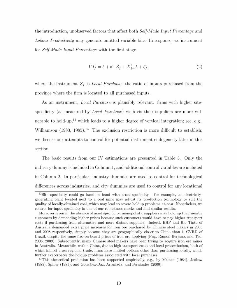
the introduction, unobserved factors that affect both Self-Made Input Percentage and

Labour Productivity may generate omitted-variable bias. In response, we instrument

for Self-Made Input Percentage with the first stage

V If = δ + θ · Zf +X ′ficλ+ ζf , (2)

where the instrument Zf is Local Purchase: the ratio of inputs purchased from the

province where the firm is located to all purchased inputs.

As an instrument, Local Purchase is plausibly relevant: firms with higher site-

specificity (as measured by Local Purchase) vis-a-vis their suppliers are more vul-

nerable to hold-up,12 which leads to a higher degree of vertical integration; see, e.g.,

Williamson (1983, 1985).13 The exclusion restriction is more difficult to establish;

we discuss our attempts to control for potential instrument endogeneity later in this

section.

The basic results from our IV estimations are presented in Table 3. Only the

industry dummy is included in Column 1, and additional control variables are included

in Column 2. In particular, industry dummies are used to control for technological

differences across industries, and city dummies are used to control for any locational

12Site specificity could go hand in hand with asset specificity. For example, an electricity-generating plant located next to a coal mine may adjust its production technology to suit thequality of locally-obtained coal, which may lead to severe holdup problems ex-post. Nonetheless, wecontrol for input specificity in one of our robustness checks and find similar results.

Moreover, even in the absence of asset specificity, monopolistic suppliers may hold up their nearbycustomers by demanding higher prices because such customers would have to pay higher transportcosts if purchasing from alternative and more distant suppliers. Indeed, BHP and Rio Tinto ofAustralia demanded extra price increases for iron ore purchased by Chinese steel makers in 2005and 2008 respectively, simply because they are geographically closer to China than is CVRD ofBrazil, despite the same free-on-board prices of iron ore applying (Png, Ramon-Berjano, and Tao,2006, 2009). Subsequently, many Chinese steel makers have been trying to acquire iron ore minesin Australia. Meanwhile, within China, due to high transport costs and local protectionism, both ofwhich inhibit cross-regional trade, firms have limited options other than purchasing locally, whichfurther exacerbates the holdup problems associated with local purchases.

13This theoretical prediction has been supported empirically, e.g., by Masten (1984), Joskow(1985), Spiller (1985), and Gonzalez-Daz, Arrunada, and Fernandez (2000).

10

advantages that may simultaneously affect local purchases, vertical integration and

firm productivity. In both columns, the IV estimate of Self-Made Input Percentage

is negative and statistically significant. In fact, the IV estimates are substantially

larger than the OLS estimates. One possibility is that the self-reported degree of

vertical integration involves some measurement errors, which biases the OLS estimates

downward (towards zero).

Instrument Relevance As shown in Panel B, Local Purchase is found to be pos-

itive and statistically significant. The Anderson canonical correlation LR statistic

and the Cragg-Donald Wald statistic (reported in Panel C) further confirm that our

instrument is relevant. The F-test of excluded instrument is statistically significant

at the 5% level, but has a value of around 5, which is below the critical value of 10

– a value suggested by Staiger and Stock (1997) as the “safety zone” for a strong

instrument. This raises possible concerns of a weak instrument for our analysis. In

response, we conduct two additional tests: the Anderson-Rubin Wald test and the

Stock-Wright LM S-statistic, which offer reliable statistical inferences under a weak

instrument setting (Anderson and Rubin, 1949; Stock and Wright, 2000). Both tests

produce statistically significant results (also reported in Panel C), implying that our

main results are robust to the presence of a weak instrument.

Instrument Exogeneity Our instrument, Local Purchase, may have causal effects

on Labour Productivity besides the vertical integration channel. Here, we identify

and control for four potential channels. First, when a firm sources more of its parts

and components locally, it may incur lower transportation costs, which subsequently

leads to higher firm productivity. Second, the shorter distance to suppliers under

local sourcing implies lower inventory requirements, leading to higher productivity.

Third, locally purchased inputs may be made to firms’ unique specifications, which

11

adds more value to their final products. Fourth, local purchases could reduce delays

in delivery and consequently minimize lost sales.

From the SCE dataset, we construct four variables corresponding to each of these

four possible alternative channels: Transportation Cost (measured by transportation

costs divided by sales), Inventory (measured by inventory stocks of final goods over

sales), Input Specificity (measured by the percentage of a firm’s inputs made to the

firm’s unique specifications) and Delivery Loss (measured by the percentage of sales

lost due to delivery delays in the previous year). We include linear and quadratic

terms for each of these channel variables. As shown in Columns 1 – 5 of Table 4,

our main results regarding the impact of vertical integration on firm productivity

remain robust to these additional controls for potential alternative channels in the IV

estimation.

Beyond these direct causal effects, the endogeneity problem still persists to some

extent: Local Purchase is itself a management choice, and thus may be correlated

with unobserved factors that also affect firm productivity.14 Such omitted-variable

bias cannot be completely excluded in our analysis, and thus constitutes a limitation

of the SCE results.

Further Robustness Checks As robustness checks, we repeat our analysis for

three subsamples. Our finding that vertical integration and firm productivity are

negatively related continues to hold in each of these subsamples.

First, to check whether our results are driven by outliers, we exclude the top and

bottom 1% of observations by firm productivity and repeat the analysis using both

OLS and IV regression methods. These results are shown in columns 1 and 2 of Table

5.

14For example, firms that are beholden to local politicians may buy more local inputs and alsoengage in excessive hiring of local workers, leading to a negative correlation between Local Purchaseand Labour Productivity. We thank an anonymous referee for highlighting this point.

12

Second, for firms with many businesses, the degree of vertical integration could

vary from one business to another. Thus, our measure of vertical integration may

reflect the average degree of vertical integration across various businesses, which may

bias our estimates of the impact of vertical integration on firm productivity. To

address this concern, we restrict attention to the subsample of firms with focused

businesses (defined as firms whose main business accounts for more than 50% of total

sales); these results are reported in Columns 3 and 4 of Table 5.

Third, China’s state-owned enterprises, as legacies of its central planning system,

are burdened with social responsibility mandates, and thus tend to be vertically

integrated and inefficient. To check that our results are not driven by state-owned

enterprises, we focus on the subsample of private firms; these results are reported in

Columns 5 and 6 of Table 5.

3 Annual Survey of Industrial Firms

The Annual Survey of Industrial Firms (ASIF) was conducted by the National Bureau

of Statistics of China during the 1998–2005 period. This is the most comprehensive

firm-level dataset in China; it covers all state-owned and non-state-owned industrial

enterprises with annual sales of at least five million Renminbi.15 The number of

firms varies from over 140,000 in the late 1990s to over 243,000 in 2005. This panel

dataset allows us to exploit within-firm time-series variation in the degree of vertical

integration. Consequently, we control for the endogeneity problem by eliminating

unobserved permanent firm heterogeneity from our regressions.

The ASIF consists of standard accounting information on firms’ operations and

performance. Our analysis of the ASIF dataset thus relies on the conventional, albeit

objective, measure of vertical integration: Value-Added Ratio. This variable has a

15As of July 2016, the exchange rate was approximately 1 Renminbi to 0.15 U.S. dollars.

13

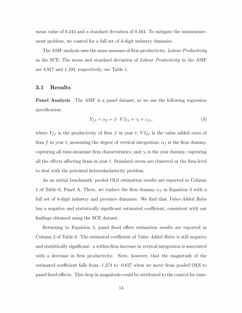
mean value of 0.244 and a standard deviation of 0.164. To mitigate the mismeasure-

ment problem, we control for a full set of 4-digit industry dummies.

The ASIF analysis uses the same measure of firm productivity, Labour Productivity

as the SCE. The mean and standard deviation of Labour Productivity in the ASIF

are 4.917 and 1.193, respectively; see Table 1.

3.1 Results

Panel Analysis The ASIF is a panel dataset, so we use the following regression

specification:

Yf,t = αf + β · V If,t + γt + εf,t, (3)

where Yf,t is the productivity of firm f in year t; V If,t is the value added ratio of

firm f in year t, measuring the degree of vertical integration; αf is the firm dummy,

capturing all time-invariant firm characteristics; and γt is the year dummy, capturing

all the effects affecting firms in year t. Standard errors are clustered at the firm-level

to deal with the potential heteroskadasticity problem.

As an initial benchmark, pooled OLS estimation results are reported in Column

1 of Table 6, Panel A. There, we replace the firm dummy αf in Equation 3 with a

full set of 4-digit industry and province dummies. We find that Value-Added Ratio

has a negative and statistically significant estimated coefficient, consistent with our

findings obtained using the SCE dataset.

Returning to Equation 3, panel fixed effect estimation results are reported in

Column 2 of Table 6. The estimated coefficient of Value Added Ratio is still negative

and statistically significant: a within-firm increase in vertical integration is associated

with a decrease in firm productivity. Note, however, that the magnitude of the

estimated coefficient falls from -1.274 to -0.627 when we move from pooled OLS to

panel fixed-effects. This drop in magnitude could be attributed to the control for time-

14

invariant firm-level unobserved characteristics (e.g., the level of transaction difficulty)

being correlated with both the degree of vertical integration and firm productivity. It

is also possible that some of the variation in the degree of vertical integration occurs

across firms rather than within firms, and thus that the within-firm variation exploited

by our panel fixed-effect estimation has a muted impact on firm productivity.

While we have controlled for all permanent firm-level unobservables through the

panel fixed-effect estimation, the endogeneity problem may persist due to time-varying

omitted-variable bias. Proxying for time-varying omitted variables using the lagged

dependent variable (Wooldridge, 2002), we estimate the following equation:

Yf,t = αf + β · V If,t + δ · Yf,t−1 + γt + εf,t. (4)

The estimation results are reported in Column 3 of Table 6. After controlling for

time-varying unobservables, the impact of vertical integration on firm productivity

remains negative and statistically significant.

Further, with the inclusion of the lagged dependent variable in the panel estima-

tion, dynamic estimation bias – whereby the lagged dependent variable is correlated

with the error term – may arise, leading to biased estimates. To address this con-

cern, we conduct a panel instrumental-variable estimation, as in Anderson and Hsiao

(1982). Specifically, in the First-Difference transformation of equation (4), we instru-

ment ∆V If,t and ∆Yf,t−1 with V If,t−1 and Yf,t−2, respectively. The Anderson-Hsiao

IV estimation results are reported in Column 4 of Table 6. Our main finding that

vertical integration has a negative impact on firm productivity continues to hold here.

Delayed Effects of Vertical integration Our analysis so far focuses on the con-

temporaneous effects of vertical integration on firm productivity. However, the effects

of vertical integration may be delayed, either because new processes associated with

15

integration and disintegration may take time to learn, or because post-integration

investments may take time to be implemented. To investigate the possibility of any

delayed effects, we further add one-year-lagged values (Panel B) and two-year-lagged

values (Panel C) of the vertical integration measure, Value Added Ratio, to our specifi-

cation. We find that the lagged effects are small relative to contemporaneous effects,

with signs that change across specifications. Further, in these specifications, our

estimates of contemporaneous effects barely change in significance and magnitude.

Overall, the estimates for contemporaneous effects seem more robust and economi-

cally more significant than the estimates for delayed effects. Our tentative interpre-

tation of these findings is that the effects of changes in vertical integration on firm

productivity are relatively contemporaneous, and are largely realized within one year.

Robustness Checks We conduct a number of robustness checks on both the panel

fixed-effect and Anderson-Hsiao IV estimation results. Our finding that vertical inte-

gration and firm productivity are negatively related continues to hold in each alter-

native specification.

To address the concern that firm entry and exit during the sample period may

drive our findings, we restrict our analysis to a balanced panel, comprising firms

present for the whole sample period (Columns 1-2 of Table 7).

Mirroring the robustness checks from the SCE analysis, we exclude the top and

bottom 1% of observations for firm productivity to check whether our results are

mainly driven by outlying observations (Columns 3-4 of Table 7). And, we exclude

state-owned enterprises by restricting our analysis to the sub-sample of private firms

(Columns 5-6 of Table 7).

Finally, to control for the endogeneity problem arising from within-industry firm

heterogeneity in technological capability (which could affect firm productivity and

ownership structure), we include Capital Intensity (measured as the logarithm of

16

assets per worker) as an additional control (Columns 7-8 of Table 7).

4 Private Enterprise Survey of Productivity and

the Investment Climate

The Private Enterprise Survey of Productivity and the Investment Climate (PESPIC)

is a standardized cross-sectional firm-level dataset based on World Bank Enterprise

Surveys (WBESs) conducted by the World Bank’s Enterprise Analysis Unit in 68

developing economies during the 2002–2006 period.16 The PESPIC’s structure is

similar to that of the SCE. The first part is a general questionaire directed at senior

management, focusing on firm structure and performance, sales and suppliers, in-

vestment and infrastructure, government relations, innovation, and labour relations.

The second part is directed at the senior accountant, and focuses on various financial

measures.

The PESPIC is cross-sectional – each firm in the dataset is surveyed only once,

sometime between 2002–2006 – but has some time-series aspects. The survey reports

many relevant time-varying firm-level variables (such as sales and employment) for

each of the previous three full fiscal years, which we label as t − 1, t − 2, and t − 3.

In particular, our dependent variable, Change in Labour Productivity, is constructed

as the change in the firm’s labour productivity over that period: that is, ∆Yf,t =

Yf,t−1 − Yf,t−3.

Importantly, the PESPIC contains a survey question designed to directly measure

changes in the degree of vertical integration: “Has your company brought in-house

major production activities in the last three years?” The reply to this survey question

is used to construct a dummy variable, Change in Vertical Integration (∆V If,t), which

16More information about the dataset can be found at http://www.enterprisesurveys.org/

17

equals 1 if the firm answers yes and 0 otherwise.

The PESPIC thus allows us to exploit within-firm variation in the degree of vertical

integration and avoid the endogeneity problem that might arise from permanent firm-

level heterogeneity. As with the SCE, the PESPIC’s measure of vertical integration

is direct and less prone to the mismeasurement problem. Further, by focusing only

on “major production activities”, the PESPIC measure is arguably less prone to

subjective interpretation by managers than the corresponding SCE measure.

As the PESPIC was compiled from a series of WBESs employing different ques-

tionnaire designs and survey methodologies in different countries, information about

the change in the sourcing strategy adopted for major production activities is avail-

able in only 6 countries (i.e., Brazil, Ecuador, Oman, the Philippines, South Africa

and Zambia). After deleting observations missing valid information about vertical in-

tegration choices, we have a final sample of 3,958 firms in these 6 developing countries.

The mean value of Change in Vertical Integration is 0.097 and the standard deviation

is 0.296. The mean and standard deviation of Change in Labour Productivity are

0.154 and 0.799, respectively; see Table 1.

4.1 PESPIC: Results

First-Difference Estimation The key independent variable in our analysis of the

cross-country PESPIC dataset is Change in Vertical Integration, which provides a

source of within-firm variation in vertical integration. We estimate the following

First-Difference equation:

∆Yf,t = α + β ·∆V If,t +X′

f,t−3γ + ∆εf,t, (5)

18

in which ∆Yf,t is the change in firm productivity, ∆V If,t is the change in the degree

of vertical integration for major production activities,17 and X′

f,t−3 is a vector of firm-

level variables (Initial Firm Size and Initial Sales Change, reflecting firm size and

year-on-year sales growth for the year t − 3). Standard errors are clustered at the

firm-level.

First-Difference estimates of equation (5) are reported in Column 1 of Table 8.

The coefficient of the Change in Vertical Integration is negative and statistically

significant, suggesting that bringing major production activities in-house leads to a

decrease in firm productivity.

While First-Difference estimation allows us to effectively control for all permanent

firm-level characteristics, the endogeneity problem could still arise from unobserved

within-firm time-varying factors. To control for such factors, we include several mea-

sures of important operational changes in the past three years as robustness checks.

The PESPIC dataset contains the following questions: (1) “Has your company

introduced any new technology that has substantially changed the way that the main

product is produced in the last three years?”; (2) “Has your company agreed any

new joint venture with a foreign partner in the last three years?”; (3) “Has your

company obtained any new licensing agreement in the last three years?”; and (4)

“Has your company developed any major new product line in the last three years?”.

Accordingly, we construct four control variables – Introduction of New Technology,

Introduction of New Joint Venture, Introduction of New Licensing Agreement, and

17Some mismatch in the time periods for ∆V If,t and ∆Yf,t may potentially arise due to ambiguityin the survey question about ∆V If,t. Specifically, the survey was conducted at some point duringfiscal year t, so – depending on the respondent’s interpretation – responses to the question (“Has yourcompany brought in-house major production activities in the last three years?”) may account forproduction changes during part of year t (up until when the survey took place). On the other hand,∆Yf,t only captures changes in productivity until the end of year t− 1; the survey does not includeinformation about productivity changes in year t. In other words, a version of the mismeasurementproblem may arise if ∆V If,t incorporates noise, in the form of “future” year-t changes in verticalintegration that should not cause ∆Yf,t.

19

Introduction of New Major Product Line – each of which takes the value of 1 if the

firm replies affirmatively to the respective question and 0 otherwise. In addition,

we construct a variable related to the change in capital intensity (i.e., measured as

the change in logarithm of assets per worker) to control for possible within-industry

heterogeneity in technology.

We include these five additional control variables in the model in a stepwise man-

ner in Columns 2-6 of Table 8. Our regressor of interest, Change in Vertical Inte-

gration, continues to produce a negative and statistically significant impact on firm

productivity, implying the robustness of our findings in Column 1 to possible time-

varying characteristics.

Robustness Checks Mirroring our robustness checks of the SCE and the ASIF, we

repeat our first-difference estimations for the following subsamples. First, we exclude

the top and bottom 1% of observations for firm productivity to check whether our

results are mainly driven by outlying observations (Column 1 of Table 9). Second,

we exclude state-owned enterprises by restricting our analysis to the sub-sample of

private firms (Column 2 of Table 9). Our main finding remains robust to these

robustness checks.

4.2 Comparing Datasets: Econometric Tradeoffs

Regarding the mismeasurement problem: the SCE and PESPIC analyses control for

the mismeasurement problem by including direct (but potentially subjective) mea-

sures of vertical integration. However, as we discuss in footnote 17, the mismeasure-

ment problem may arise in the PESPIC from a different source: ambiguity about

the time period over which the independent variable, Change in Vertical Integration,

is reported. The ASIF analysis relies on Value Added as a measure of vertical inte-

20

gration, which is susceptible to the mismeasurement problem; this issue is partially

alleviated by our inclusion of a detailed set of 4-digit industry dummies (and, in some

specifications, firm dummies).

Regarding the endogeneity problem: for the cross-sectional analysis of the SCE,

we are concerned with firm-level heterogeneity. We utilize Local Purchase as an

instrument for vertical integration, and control for a large set of variables including

industry dummies, city dummies and CEO and firm characteristics. In particular, we

attempt to identify and control for potential channels through which Local Purchase

may have causal effects on Labour Productivity. Nonetheless, we cannot completely

exclude the possibility that omitted-variable bias (either permanent or time-varying)

affects our IV results. The ASIF and PESPIC datasets allow us to conduct panel

analyses that control for permanent firm-level heterogeneity, but cannot completely

eliminate potential firm-specific time-varying shocks that may drive both vertical

integration decisions and firm productivity.

5 A Simple Model: Vertical Integration, Rent-

Seeking, and Firm Performance

This section presents a simple and very stylised model of vertical integration. In

the model, integration corresponds to firm insiders (e.g. firm management) retaining

key decision-rights that determine the outcome of production, whereas outsourcing

corresponds to the partial transfer of decision rights to outside suppliers.

As a quick preview: the key source of inefficiency in the model is that integration

gives insiders more control over the production process, and thus enables their rent-

seeking activities. Outsourcing, by reducing insider control, reduces incentives for

such rent-seeking because the returns to rent-seeking have to be shared between in-

21

siders and suppliers. The dark side of outsourcing is that it also suppresses managerial

incentives for productive but costly actions.

Our model assumes that rent-seeking benefits accrue to the insider, and that

ex-post bargaining over the implementation of actions is efficient. We relax these

assumptions in the Appendix, and show that our qualitative results continue to hold.

There is a single insider (who we may think of as an entrenched CEO, or the

firm’s majority shareholder), and a unit mass of infinitesimally-weighted tasks to be

managed. Each task is assigned a manager, and requires some task-specific assets.

Mass m ∈ (0, 1) of tasks are integrated: the insider manages the task, and the firm

owns the task-specific assets. The remaining 1−m tasks are outsourced: an outside

supplier manages the task, and owns the task-specific assets. Outside suppliers are

specialized, so each supplier can manage a maximum of one (infinitesimal) task for

the firm. Each task θ produces net revenue πθ, which we specify later and takes into

account action costs and / or transfers to the supplier. Firm revenue equals net task

revenue integrated over all tasks:

Π =

∫ 1

0

πθdθ. (6)

The insider receives fraction b ∈ (0, 1) of total revenue Π,18 as well as some private

benefits to be specified later. Revenue πθ and private benefits are not contractible,

so formal incentive contracts cannot be offered to outside suppliers.19

For each task θ, there are two costly, noncontractible actions chosen by the task’s

18Think of the remaining share of revenue as going to passive shareholders who have no say infirm decision-making.

19We may allow for a verifiable, noisy signal of firm revenue y = Π + ε to be available. However,because each task is infinitesimal, firm revenue would be uncorrelated with revenue from each task,and thus incentive contracts for suppliers based on firm revenue would be ineffective. The premiseis that because there are many suppliers who each make only a small contribution to firm revenue,incentive provision based on firm revenue becomes prohibitively costly, especially in the presence ofcontracting frictions such as supplier risk-aversion.

22

manager: a productive action pθ ≥ 0 that increases firm revenue, and a rent-seeking

action rθ ≥ 0 that produces private benefits for the insider at the expense of firm

revenue. These actions have to be implemented, and implementation requires the

cooperation of the insider; the underlying premise is that insourcing of task θ corre-

sponds to the insider having sole control over θ, whereas outsourcing corresponds to

joint control by insider and supplier. Specifically, if actions pθ and rθ are successfully

implemented, then gross task revenue is pθ−rθ while the insider receives rθ in private

benefits from that task. If implementation fails, then gross task revenue and private

benefits equal zero.

The cost of these actions cθ = 12p2θ + 1

2αr2θ is incurred by the owner of the task-

specific assets: the firm for integrated tasks, and the supplier for outsourced tasks.

Parameter α represents the ease of expropriation: higher α represents weaker legal

protections which allow the player performing the task to expropriate from the firm

more easily.

The overall timing of the model is as follows:

1. For each outsourced task θ, the insider makes the outside supplier a participation

offer κθ ∈ R. If the supplier accepts, then he receives κθ from the firm;20

otherwise the task is not performed, and the supplier receives an outside option

payoff normalized to zero.

2a. For each task θ, the manager (the insider under integration, the supplier under

outsourcing) chooses costly actions pθ and rθ, and cost cθ is sunk.

2b. For each outsourced task θ, the insider bargains with the supplier over (i)

whether to implement the action, and (ii) a transfer µθ ∈ R from firm to

20If κθ < 0, then the payment is from the supplier to the firm.

23

supplier.21 Assume efficient Nash bargaining, so the insider and supplier share

the bargaining surplus equally.

Notice that the manager’s costly, noncontractible actions are taken ex-ante, with

ex-post efficient bargaining over implementation of these actions. In interpreting the

model, we are agnostic about the time span over which these noncontractible actions

are made and implemented: they may be long-term investments (e.g., human capital

investments) or short-term choices (e.g., choosing the quality of raw materials pur-

chased). Further, the efficient ex-post bargaining step is not crucial to our results:

in the Appendix, we consider an alternative assumption where the non-contractible

actions are taken ex-post (with no subsequent bargaining), and show that our qual-

itative findings remain unchanged. This alternative assumption may better capture

settings where decisions are implemented rapidly and thus have relatively contempo-

raneous effects on output.22

To recap, we summarize some key quantities. Net task revenue accounts for action

costs under integration, and transfers to the supplier under outsourcing:

πθ =

pθ − rθ − cθ under integration,

pθ − rθ − (κθ + µθ) under outsourcing.

(7)

The insider’s payoff u consists of her share of firm revenue, plus private benefits:

u = bΠ +

∫ 1

0

rθ dθ =

∫ 1

0

(bπθ + rθ) dθ.

21Our results remain qualitatively unchanged if we assume that payments are made “under-the-table”, between insider and supplier; such a change simply corresponds to a shift in relative bar-gaining power between the two parties.

22One interpretation of our finding in Section 3 – that the effects of vertical integration arerelatively contemporaneous – is that, at least in some settings, the relevant noncontractible actionsare short-run in nature.

24

Each outsourcing supplier’s payoff vθ is his net transfer, less action costs:

vθ = κθ + µθ − cθ.

Total surplus is gross revenue, plus private benefits, less action costs cθ:

surplus =

∫ 1

0

[pθ −

(1

2p2θ +

1

2αr2θ

)]dθ.

Note that the first-best (surplus maximization) is achieved when pθ ≡ 1 and rθ ≡ 0.

5.1 Integration versus Outsourcing

We start with a convenient observation which allows for a straightforward comparison

between integration and outsourcing. An asterisk denotes equilibrium outcomes; for

example, c∗θ denotes the equilibrium level of cθ.

Lemma 1. In equilibrium, under both integration and outsourcing, net task revenue

equals gross task revenue less action cost cθ:

π∗θ = (p∗θ − r∗θ)−(

1

2p∗2θ +

1

2αr∗2θ

). (8)

Proof. In the case of integration, (8) is simply a restatement of (7). In the case of

outsourcing, note that in step 1, the insider maximizes his payoff for task θ by mini-

mizing the payment κθ. The insider thus holds the supplier to his zero outside option

in equilibrium, so that the supplier is indifferent between accepting and rejecting the

step 1 offer: v∗θ = κ∗θ + µ∗θ − c∗θ = 0. (In words, the equilibrium net transfer κ∗θ + µ∗θ to

the supplier equals the equilibrium action cost c∗θ.) Substituting this expression into

(7), we get (8).

The next two lemmas calculate the equilibrium actions under integration and

25

outsourcing. Denote equilibrium outcomes under integration (resp. outsourcing)

with a subscript I (resp. S); for example, net task revenue for an integrated task is

denoted as π∗I .

Lemma 2. Suppose task θ is integrated. Then the insider chooses p∗I = 1 and r∗I =

α 1−bb

for that task. Net task revenue is π∗I = 12− α 1−b2

2b2.

Proof. Under integration, the insider chooses pθ and rθ to maximize his payoff b(pθ−

rθ − 12p2θ − 1

2αr2θ) + rθ, i.e. p∗I = 1 and r∗I = α(1−b)

b. Net revenue for the task is thus

p∗I − r∗I − 12p∗2I − 1

2αr∗2I = 1

2− α 1−b2

2b2.

Under integration, the insider appropriately internalizes the costs and benefits of

the productive action, and chooses the first-best productive action p∗θ = 1. On the

other hand, because she appropriates all benefits from rent-seeking but only bears

fraction b < 1 of the costs, she engages in inefficient rent-seeking. This rent-seeking

action, and the resultant inefficiency, is increasing in the ease of expropriation α.

Lemma 3. Suppose task θ is outsourced. Then the supplier for that task chooses

p∗S = b1+b

and r∗S = α 1−b1+b

. Net revenue from the task is π∗S = b1+b

2+b2+2b− α 1−b

1+b3+b2+2b

.

Proof. The insider’s disagreement payoff is −bκθ, while the supplier’s disagreement

payoff is κθ − 12p2θ − 1

2αr2θ . On the other hand, given a bargaining payment µθ (paid

by the firm) to the supplier, the insider’s payoff (following implementation) is b(pθ −

rθ − µθ − κθ) + rθ, while the supplier’s payoff becomes κθ + µθ − 12p2θ − 1

2αr2θ . The

two parties Nash bargain to an equal-surplus outcome: bpθ + (1 − b)rθ − bµθ = µθ.

Solving for the bargaining payment, µθ = bpθ+(1−b)rθ1+b

; so the supplier’s net payoff is

κθ + bpθ+(1−b)rθ1+b

− 12p2θ − 1

2αr2θ . To maximize this payoff, the supplier chooses actions

p∗S = b1+b

and r∗S = α 1−b1+b

. Net revenue from task θ is thus π∗S = p∗S−r∗S− 12p∗2S − 1

2αr∗2S =

b1+b

2+b2+2b− α 1−b

1+b3+b2+2b

.

26

Compared to the insider’s choices under integration, the (supplier’s) productive

and rent-seeking actions under outsourcing are each diminished by a factor b1+b

.23

Under outsourcing, the supplier has to share the returns from his productive and rent-

seeking actions with the insider; thus his incentives for both actions are suppressed

relative to the insider’s incentives under integration, where the insider keeps the “full”

returns from his actions.

The tradeoff between integration and outsourcing is thus as follows: integration

increases productive actions (p∗I > p∗S), but also results in more costly rent-seeking

(r∗I > r∗S). An increase in the ease of expropriation α increases the extent of rent-

seeking, and consequently makes outsourcing more profitable relative to integration.

Proposition 1. Firm revenue Π is increasing in the extent of integration m if

α <b2

(1− b)(1 + 3b), (9)

and decreasing in m otherwise.

Proof. From Lemmas 2 and 3, integrated tasks contribute π∗I = 12− α 1−b2

2b2of revenue

per unit mass, whereas outsourced tasks contribute π∗S = b1+b

2+b2+2b− α 1−b

1+b3+b2+2b

of rev-

enue per unit mass. Mass m of tasks are integrated and mass 1−m are outsourced,

so firm revenue is Π = mπ∗I + (1 − m)π∗S = π∗S + m (π∗I − π∗S). Consequently, Π is

increasing in m if and only if π∗I − π∗S > 0. Using the expressions for π∗I and π∗S

from Lemmas 2 and 3, some manipulations reveal that this is the case if and only if

α < b2

(1−b)(1+3b).

Thus integration is more profitable than outsourcing if and only if the ease of

23Note that if transfers were paid by the manager (rather than the firm) to the supplier, then thesupplier’s incentives would instead by diminished by a factor 1

2 . This assumption corresponds to asetting where ex-post renegotiation takes place under-the-table, with bribes paid by the insider tothe supplier. The results do not change qualitatively in this alternative setting.

27

expropriation α is small.24

In other words: the effect of an increase in the degree of firm integration on revenue

depends on the quality of the legal environment. In good (bad) legal environments

where expropriation is difficult (easy), an increase in firm integration results in an

increase (decrease) in firm revenue and total surplus. In particular, the case of high α

matches our setting of China and other developing countries, where legal protections

are relatively weak and expropriation is easy. In that case, Proposition 1 predicts

that firm productivity (as measured by revenue) is decreasing in the degree of vertical

integration. This matches our empirical findings.

5.2 Managerial Ability and the Integration Decision

So far, we have exogenously specified the degree of integration m.25 We now allow the

insider to choose m at the start of the game (i.e., before step 1). To introduce variation

in the integration decision across firms, suppose that insiders differ in managerial

ability: more capable insiders can easily handle more tasks via integration without

relying on suppliers. To model the difficulty of managing integration, suppose that

the insider incurs a private cost of integration C(m) = m2

2η, where η ≥ 0 captures the

manager’s ability.

Proposition 2. The equilibrium degree of integration m∗ is increasing in managerial

ability η and in the ease of expropriation α. Further, firm revenue Π is increasing

24Similarly, we may show that total surplus (revenue plus managerial and supplier payoffs) isincreasing in the degree of integration if and only if α is small, i.e., expropriation is difficult. Each

task θ produces surplus pθ − p2θ/2 − r2θ/(2α). In particular, integrated tasks produce 12 −

(1−b)2α2b2

of surplus per unit mass, and outsourced tasks produce b(2+b)2(1+b)2 −

α(1−b)22(1+b)2 of surplus per unit mass.

Consequently, total surplus is m(

12 −

(1−b)2α2b2

)+ (1−m)

(b(2+b)2(1+b)2 −

α(1−b)22(1+b)2

), which is increasing in

m if and only if α < b2

(1+2b)(1−b)2 .25We also assume that the insider’s share of revenue b ∈ (0, 1) is exogenously specified. In fact,

firm revenue Π would be maximized at the upper bound b = 1, in which case the insider is a residualclaimant. We adopt the premise that b is limited by exogenous factors such as wealth constraintson the insider’s shareholdings.

28

in η (and thus with m∗) if α < b2

(1−b)(1+3b), and is decreasing in η (and thus with m∗)

otherwise.

Proof. The insider’s payoff if mass m of tasks are integrated is m(bπ∗I + r∗I ) + (1 −

m)(bπ∗S+r∗S)−m2

2η, which we may rewrite as bπ∗S+r∗S+m (b(π∗I − π∗S) + (r∗I − r∗S))−m2

2η;

so the insider optimally chooses m∗ = min{1, η (b(π∗I − π∗S) + (r∗I − r∗S))}. Note that

m∗ is increasing in managerial ability η (strictly so if m∗ ∈ (0, 1)). Further, some

manipulations reveal that

b(π∗I − π∗S) + (r∗I − r∗S) =b

2(1 + b)2+ α

3(1− b)2(1 + b)2

(10)

is increasing in the ease of expropriation α; thus, so is m∗. Now, because the cost m2

2η

is privately borne by the insider, the expression for equilibrium firm revenue remains

unchanged from Section 5.1: Π∗ = m∗π∗I + (1 −m∗)π∗S. The result of Proposition 2

thus follows from Proposition 1.

Proposition 2 states that more capable insiders can handle more integrated tasks

without relying on suppliers, and thus choose a greater degree of integration for the

firms they manage. The effect on firm productivity of this increased integration

depends on whether the insider invests more in productive or rent-seeking activities.

In particular, in poor legal environments (high α), high-ability managers actually

decrease firm-level productivity, because they apply their capabilities towards rent-

seeking rather than productive activities. (But their ability only affects m here. There

may be counter-acting forces.)

Proposition 2 predicts that revenue increases with integration m if and only if

expropriation is easy: α < b2

(1−b)(1+3b). The threshold for α is identical to that of

Proposition 1, which considers the effect of an exogenous shift in m on firm revenue.

This is because the integration cost – being privately incurred by the insider – affects

29

firm revenue only via the choice of m, and is otherwise orthogonal to the production

function (7). In the Appendix, we consider a simple variation of the model where

managerial ability directly affects the revenue from integrated tasks, and show that

our predictions remain qualitatively unchanged.

Further, Proposition 2 highlights two countervailing forces that may drive equilib-

rium integration decisions in developing countries. Poor corporate governance (high

α) produces more integration, because insiders integrate more tasks to take advan-

tage of easier rent-seeking. On the other hand, a relative dearth of managerial talent

(low η) in developing economies may result in less integration. Consequently, taking

both forces into account, the effect on equilibrium integration m∗ of moving from a

developed-country to a developing-country setting is ambiguous.

6 Conclusion

This paper investigates the impact of vertical integration on firm productivity using

firm-level data from China and other developing countries. Mismeasurement and

endogeneity problems pose challenges in this line of research. Our approach is to

analyze, separately, three different datasets that address the mismeasurement and

endogeneity problems in different ways. Throughout our analysis, we consistently

find that the degree of vertical integration has a negative and statistically significant

impact on firm productivity. This consistency, as well as the cross-industry nature

of our samples, suggests that our findings may be quite broadly applicable to the

developing-country context.

Our results contrast with recent empirical findings (largely based on U.S. firms)

that vertical integration is positively correlated with firm productivity. We propose

that the differences between their results and ours are driven by differences in the

ease of rent-seeking in developed versus developing countries. In particular, weak

30

legal environments complement integrated firm structures in enabling rent-seeking

by firm insiders, so the costs of integration outweigh the benefits of integration in

developing countries where legal protections are weak.

31

7 Appendix: Model Extensions and Robustness

This appendix considers three variants of the basic model. It shows that our basic re-

sults remain qualitatively robust to these modifications. In particular, the basic force

animating the model remains the same. Integration provides stronger incentives than

outsourcing for both productive and rent-seeking actions, because integration gives

sole control to the decision-maker (insider), whereas outsourcing forces the decision-

maker (supplier) to share control with the insider. Consequently, task revenue is

higher under integration than outsourcing if and only if the ease of expropriation α

is low.

To simplify the expressions, assume without loss that given degree of integration

m, tasks θ ∈ [0,m) are integrated and tasks θ ∈ [m, 1] are outsourced.

Manager-Specific Private Benefits Section 5 assumes that regardless of the

integration decision, all private benefits from rent-seeking activities accrue to the

insider. This seems natural, as an entrenched insider would likely have more avenues

than outside suppliers to enjoy the fruits of rent-seeking activities, such as managerial

perks or expense accounts. That said, we consider below the alternative assumption

that private benefits always accrue to the manager of the task (i.e., by the insider

under integration, and by the supplier under outsourcing); so that suppliers’ and

insider’s payoffs become

vθ = rθ + κθ + µθ − cθ,

u = bΠ +

∫ m

0

rθ dθ.

This change affects the outcome of ex-post bargaining and thus the supplier’s incen-

tives to invest under outsourcing. However, p∗I and r∗I remain unchanged.

32

Proposition 3. With manager-specific private benefits: under outsourcing, p∗S = b1+b

and r∗S = 0. Consequently, p∗I > p∗S and r∗I > r∗S. Further, firm revenue Π is increasing

in m if and only if α < b2

(1−b)(1+b)3 .

Proof. The insider’s disagreement payoff is −bκθ, while the supplier’s disagreement

payoff is κθ − 12p2θ − 1

2αr2θ . On the other hand, given a bargaining payment µθ (paid

by the firm) to the supplier, the insider’s payoff (following implementation) is b(pθ −

rθ − µθ − κθ), while the supplier’s payoff becomes rθ + κθ + µθ − 12p2θ − 1

2αr2θ . The

two parties Nash bargain to an equal-surplus outcome: bpθ − brθ − bµθ = rθ + µθ.

Solving for the bargaining payment, µθ = bpθ−(1+b)rθ1+b

; so the supplier’s net payoff is

κθ + bpθ1+b− 1

2p2θ − 1

2αr2θ . To maximize this payoff, the supplier chooses p∗S = b

1+band

r∗S = 0. Net revenue from task θ is thus π∗S = p∗S− r∗S− 12p∗2S − 1

2αr∗2S = b

1+b2+b2+2b

. Using

this and the fact from Lemma 2 that π∗I = 12− α 1−b2

2b2, some further manipulations

show that firm revenue Π = π∗S + m (π∗I − π∗S) is increasing in m if and only if α <

b2

(1−b)(1+b)3 .

Ex-Post Decision-Making Section 5 assumes that the costly actions pθ, rθ are ex-

ante investments, and that ex-post bargaining over implementation of those actions

takes place for outsourced tasks. An alternative modelling approach is to posit that

efficient bargaining over implementation does not take place. Specifically, assume

that in step 2b, no transfers are allowed and the insider simply decides whether to

implement the actions pθ and rθ. If not, then the outcome is zero task revenue and

private benefits.

In this setting, we may think of steps 2a and 2b as an ex-post adaptation stage,

with joint control over decision-making by insider and supplier. One interpretation

may be that the time window for steps 2a and 2b is short, so that renegotiation is

infeasible. Thus it may better capture the premise of short-run decision-making than

does the setting of Section 5.

33

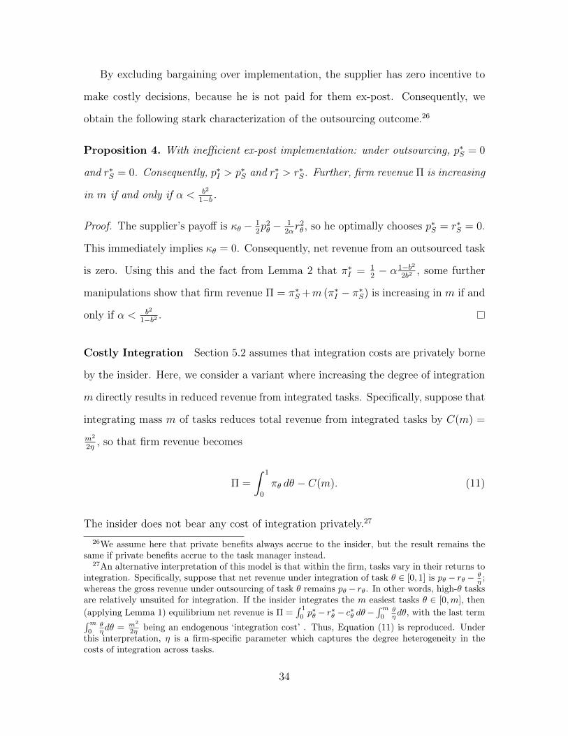
By excluding bargaining over implementation, the supplier has zero incentive to

make costly decisions, because he is not paid for them ex-post. Consequently, we

obtain the following stark characterization of the outsourcing outcome.26

Proposition 4. With inefficient ex-post implementation: under outsourcing, p∗S = 0

and r∗S = 0. Consequently, p∗I > p∗S and r∗I > r∗S. Further, firm revenue Π is increasing

in m if and only if α < b2

1−b .

Proof. The supplier’s payoff is κθ − 12p2θ − 1

2αr2θ , so he optimally chooses p∗S = r∗S = 0.

This immediately implies κθ = 0. Consequently, net revenue from an outsourced task

is zero. Using this and the fact from Lemma 2 that π∗I = 12− α 1−b2

2b2, some further

manipulations show that firm revenue Π = π∗S +m (π∗I − π∗S) is increasing in m if and

only if α < b2

1−b2 .

Costly Integration Section 5.2 assumes that integration costs are privately borne

by the insider. Here, we consider a variant where increasing the degree of integration

m directly results in reduced revenue from integrated tasks. Specifically, suppose that

integrating mass m of tasks reduces total revenue from integrated tasks by C(m) =

m2

2η, so that firm revenue becomes

Π =

∫ 1

0

πθ dθ − C(m). (11)

The insider does not bear any cost of integration privately.27

26We assume here that private benefits always accrue to the insider, but the result remains thesame if private benefits accrue to the task manager instead.

27An alternative interpretation of this model is that within the firm, tasks vary in their returns tointegration. Specifically, suppose that net revenue under integration of task θ ∈ [0, 1] is pθ − rθ − θ

η ;whereas the gross revenue under outsourcing of task θ remains pθ − rθ. In other words, high-θ tasksare relatively unsuited for integration. If the insider integrates the m easiest tasks θ ∈ [0,m], then

(applying Lemma 1) equilibrium net revenue is Π =∫ 1

0p∗θ − r∗θ − c∗θ dθ−

∫m0

θηdθ, with the last term∫m

0θηdθ = m2

2η being an endogenous ‘integration cost’ . Thus, Equation (11) is reproduced. Underthis interpretation, η is a firm-specific parameter which captures the degree heterogeneity in thecosts of integration across tasks.

34

The main point of this variant is that the comparative statics from Proposition

2 continue to hold qualitatively: higher-ability managers integrate more tasks, and

firm revenue increases (decreases) with the degree of integration m for low (high) α.

Proposition 5. Under costly integration, the equilibrium degree of integration m∗ is

increasing in managerial ability η and in the ease of expropriation α. Further, firm

revenue π is increasing in η (and thus with m∗) if α < b2

3(1+b), and is decreasing in η

(and thus with m∗) otherwise.

Proof. First, note that in this setting, the expressions for equilibrium task revenue, π∗I

and π∗S, remain unchanged from the basic model. Given m, firm revenue is Π = mπI+

(1−m)πS−m2

2η, and the insider’s payoff is m(bπ∗I +r∗I )+(1−m)(bπ∗S+r∗S)−bm2

2η, which

we may rewrite as bπ∗S +r∗S +m (bπ∗ + r∗)− bm2

2ηwhere π∗ = π∗I −π∗S and r∗ = r∗I −r∗S.

The insider optimally chooses m∗ = η(π∗ + r∗

b

). From Equation (10), π∗+ r∗

b> 0, so

m∗ is increasing in η. Thus, firm revenue is π∗S + m∗ π∗ − m∗2

2η= π∗S + η

2

(π∗2 − r∗2

b2

).

Again, π∗ + r∗

b> 0, so firm revenue is increasing in η iff π∗ − r∗

b= b

2(1+b)2− α 3(1+b)

2b(1+b)2

is positive; i.e., iff α < b2

3(1+b).

35

References

Anderson, T. W., and C. Hsiao (1982): “Formulation and estimation of dynamicmodels using panel data,” Journal of Econometrics, 18(1), 47–82.

Anderson, T. W., and H. Rubin (1949): “Estimation of the Parameters of aSingle Equation in a Complete System of Stochastic Equations,” The Annals ofMathematical Statistics, 20(1), 46–63.

Atalay, E., A. Hortacsu, and C. Syverson (2014): “Vertical Integration andInput Flows,” The American Economic Review, 104(4), 1120–1148.

Bai, C.-E., Y. Du, Z. Tao, and S. Y. Tong (2004): “Local protectionism andregional specialization: evidence from China’s industries,” Journal of InternationalEconomics, 63(2), 397–417.

Bai, C.-E., D. D. Li, Z. Tao, and Y. Wang (2000): “A Multitask Theory ofState Enterprise Reform,” Journal of Comparative Economics, 28(4), 716–738.

Chipty, T. (2001): “Vertical Integration, Market Foreclosure, and Consumer Wel-fare in the Cable Television Industry,” The American Economic Review, 91(3),428–453.

David, G., E. Rawley, and D. Polsky (2013): “Integration and Task Allocation:Evidence from Patient Care,” Journal of Economics & Management Strategy, 22(3),617–639.

Forbes, S. J., and M. Lederman (2010): “Does vertical integration affect firmperformance? Evidence from the airline industry,” The RAND Journal of Eco-nomics, 41(4), 765–790.

Gibbons, R. (2005): “Four formal(izable) theories of the firm?,” Journal of Eco-nomic Behavior & Organization, 58(2), 200–245.

Gil, R. (2009): “Revenue Sharing Distortions and Vertical Integration in the MovieIndustry,” Journal of Law, Economics, and Organization, 25(2), 579–610.

(2015): “Does Vertical Integration Decrease Prices? Evidence from theParamount Antitrust Case of 1948,” American Economic Journal: Economic Pol-icy, 7(2), 162–191.

Gonzalez-Daz, M., B. Arrunada, and A. Fernandez (2000): “Causes of sub-contracting: evidence from panel data on construction firms,” Journal of EconomicBehavior & Organization, 42(2), 167–187.

Holmes, T. J. (1999): “Localization of Industry and Vertical Disintegration,” TheReview of Economics and Statistics, 81(2), 314–325.

36

Hortacsu, A., and C. Syverson (2007): “Cementing Relationships: VerticalIntegration, Foreclosure, Productivity, and Prices,” Journal of Political Economy,115(2), 250–301.

Joskow, P. L. (1985): “Vertical Integration and Long-Term Contracts: The Caseof Coal-Burning Electric Generating Plants,” Journal of Law, Economics, and Or-ganization, 1(1), 33–80.

Levin, R. C. (1981): “Vertical integration and profitability in the oil industry,”Journal of Economic Behavior & Organization, 2(3), 215–235.

Masten, S. E. (1984): “The Organization of Production: Evidence from theAerospace Industry,” The Journal of Law and Economics, 27(2), 403.

Mullainathan, S., and D. Scharfstein (2001): “Do Firm Boundaries Matter?,”The American Economic Review, 91(2), 195–199.

Png, I., C. Ramon-Berjano, and Z. Tao (2006): “BHP: Negotiating Iron OrePrices With China,” Asia Case Research Centre, The University of Hong Kong,06(315C).

(2009): “Rio Tinto: Takeover Fears and Price Negotiations with China,”Asia Case Research Centre, The University of Hong Kong, 09(415C).

Spiller, P. T. (1985): “On Vertical Mergers,” Journal of Law, Economics, andOrganization, 1(2), 285–312.

Staiger, D., and J. H. Stock (1997): “Instrumental Variables Regression withWeak Instruments,” Econometrica, 65(3), 557.

Stock, J. H., and J. H. Wright (2000): “GMM with Weak Identification,”Econometrica, 68(5), 1055–1096.

Williamson, O. E. (1983): “Credible Commitments: Using Hostages to SupportExchange,” The American Economic Review, 73(4), 519–540.

(1985): The Economic Institutions of Capitalism. New York : Free Press ;London : Collier Macmillan Publishers.

Wooldridge, J. M. (2002): Econometric analysis of cross section and panel data.Cambridge, Mass. : MIT Press.

Young, A. (2000): “The Razor’s Edge: Distortions and Incremental Reform in thePeople’s Republic of China,” The Quarterly Journal of Economics, 115(4), 1091–1135.

37

Table 1: Summary Statistics Variable Obs Mean Std.Dev. Min Max SCEDatasetLabourProductivity 1557 4.322 1.562 -3.989 11.893Vertical Integration 1459 0.339 0.401 0.000 1.000 ASIFDatasetLabourProductivity 1115452 4.917 1.193 -8.120 13.017Vertical Integration 1016918 0.244 0.164 0.000 1.000 PESPICDatasetChangeinLabourProductivity 6212 0.154 0.799 -8.177 13.080ChangeinVertical Integration 31107 0.097 0.296 0.000 1.000

Table 2: Analysis of the SCE Dataset, OLS Benchmark

1 2 3 4 Dependent Variable Labour Productivity Self-Made Input Percentage -0.307*** -0.278*** -0.298*** -0.237*** [0.100] [0.079] [0.079] [0.086] Firm Characteristics Firm Size 0.200*** 0.181*** 0.110*** [0.037] [0.038] [0.036] Firm Age -0.526*** -0.458*** -0.413*** [0.062] [0.069] [0.066] Percentage of Private Ownership 0.442*** 0.253* 0.268** [0.130] [0.132] [0.122] Capital Intensity 0.383*** 0.384*** 0.347*** [0.037] [0.034] [0.036] CEO Characteristics Human Capital Education 0.041*** 0.040** [0.016] [0.016] Years of Being CEO 0.018** 0.007 [0.007] [0.007] Deputy CEO Previously -0.004 -0.008 [0.070] [0.068] Political Capital Government Cadre Previously 0.019 0.090 [0.222] [0.231] Communist Party Member -0.192** -0.096 [0.082] [0.077] Government Appointment -0.348*** -0.317*** [0.088] [0.092] Industry Dummy Yes Yes Yes Yes City Dummy Yes No. of Observation 1,451 1,431 1,410 1,410

Robust standard errors, clustered at industry-city level, are reported in the bracket. *, **, and *** represent significance at 10%, 5%, and 1% level, respectively.

Table 3: Analysis of the SCE Dataset, IV Estimates

1 2 Panel A, Second Stage: Dependent Variable is Labour Productivity

Self-Made Input Percentage -13.290** [6.360] -5.182* [2.803] Firm Characteristics Firm Size 0.180*** [0.063] Firm Age -0.291** [0.127] Percentage of Private Ownership 0.371 [0.234] Capital Intensity 0.323*** [0.054]

CEO Characteristics: Human Capital Education 0.061** [0.030] Years of Being CEO 0.033* [0.020] Deputy CEO Previously 0.096 [0.146]

CEO Characteristics: Political Capital Government Cadre Previously -0.451 [0.448] Communist Party Membership -0.24 [0.180] Government Appointment -0.408** [0.173] Industry Dummy Yes Yes City Dummy Yes

Panel B, First Stage: Dependent Variable is Self-Made Input Percentage Local Purchase 0.066** [0.030] 0.067** [0.029] Firm Characteristics Firm Size 0.016* [0.009] Firm Age 0.021 [0.018] Percentage of Private Ownership 0.019 [0.033] Capital Intensity -0.003 [0.008]

CEO Characteristics: Human Capital Education 0.005 [0.005] Years of Being CEO 0.005** [0.003] Deputy CEO Previously 0.025 [0.025]

CEO Characteristics: Political Capital Government Cadre Previously -0.105* [0.059] Communist Party Membership -0.029 [0.030] Government Appointment -0.022 [0.025] Industry Dummy Yes Yes City Dummy Yes

Panel C, Various First-Stage Statistical Tests Relevance Test Anderson Canonical Correlation LR Statistic [4.96]** [4.57]** Cragg-Donald Wald Statistic [4.83]** [4.48]** Weak Instrument Test F Test of Excluded Instrument [4.95]** [5.25]** Anderson-Rubin Wald Test [43.67]*** [9.13]*** Stock-Wright LM S Statistic [23.07]*** [8.05]***

Number of Observations 1,445 1,404 Note: Robust standard errors, clustered at industry-city level, are presented in the bracket. *, **, *** represent significance at 10%, 5%, 1% level respectively.

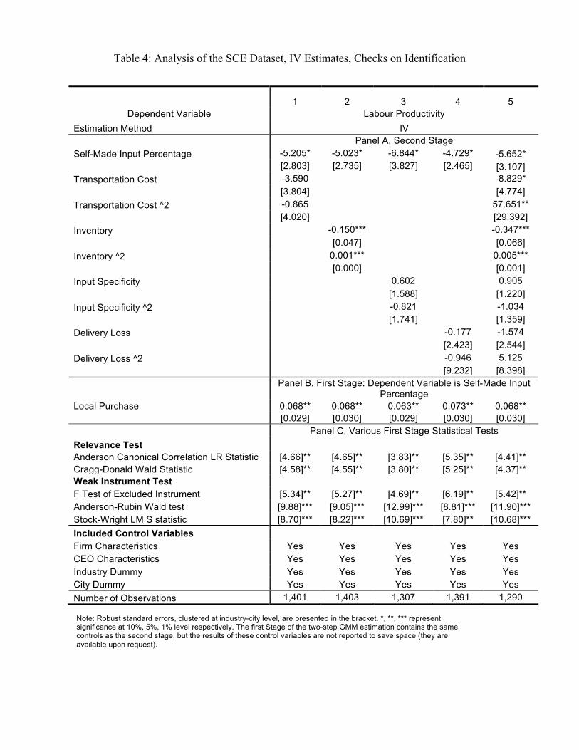
Table 4: Analysis of the SCE Dataset, IV Estimates, Checks on Identification

Note: Robust standard errors, clustered at industry-city level, are presented in the bracket. *, **, *** represent significance at 10%, 5%, 1% level respectively. The first Stage of the two-step GMM estimation contains the same controls as the second stage, but the results of these control variables are not reported to save space (they are available upon request).

1 2 3 4 5 Dependent Variable Labour Productivity

Estimation Method IV Panel A, Second Stage Self-Made Input Percentage -5.205* -5.023* -6.844* -4.729* -5.652* [2.803] [2.735] [3.827] [2.465] [3.107] Transportation Cost -3.590 -8.829* [3.804] [4.774] Transportation Cost ^2 -0.865 57.651** [4.020] [29.392] Inventory -0.150*** -0.347*** [0.047] [0.066] Inventory ^2 0.001*** 0.005*** [0.000] [0.001] Input Specificity 0.602 0.905 [1.588] [1.220] Input Specificity ^2 -0.821 -1.034 [1.741] [1.359] Delivery Loss -0.177 -1.574 [2.423] [2.544] Delivery Loss ^2 -0.946 5.125 [9.232] [8.398]

Panel B, First Stage: Dependent Variable is Self-Made Input

Percentage Local Purchase 0.068** 0.068** 0.063** 0.073** 0.068** [0.029] [0.030] [0.029] [0.030] [0.030] Panel C, Various First Stage Statistical Tests Relevance Test Anderson Canonical Correlation LR Statistic [4.66]** [4.65]** [3.83]** [5.35]** [4.41]** Cragg-Donald Wald Statistic [4.58]** [4.55]** [3.80]** [5.25]** [4.37]** Weak Instrument Test F Test of Excluded Instrument [5.34]** [5.27]** [4.69]** [6.19]** [5.42]** Anderson-Rubin Wald test [9.88]*** [9.05]*** [12.99]*** [8.81]*** [11.90]*** Stock-Wright LM S statistic [8.70]*** [8.22]*** [10.69]*** [7.80]** [10.68]*** Included Control Variables Firm Characteristics Yes Yes Yes Yes Yes CEO Characteristics Yes Yes Yes Yes Yes Industry Dummy Yes Yes Yes Yes Yes City Dummy Yes Yes Yes Yes Yes Number of Observations 1,401 1,403 1,307 1,391 1,290

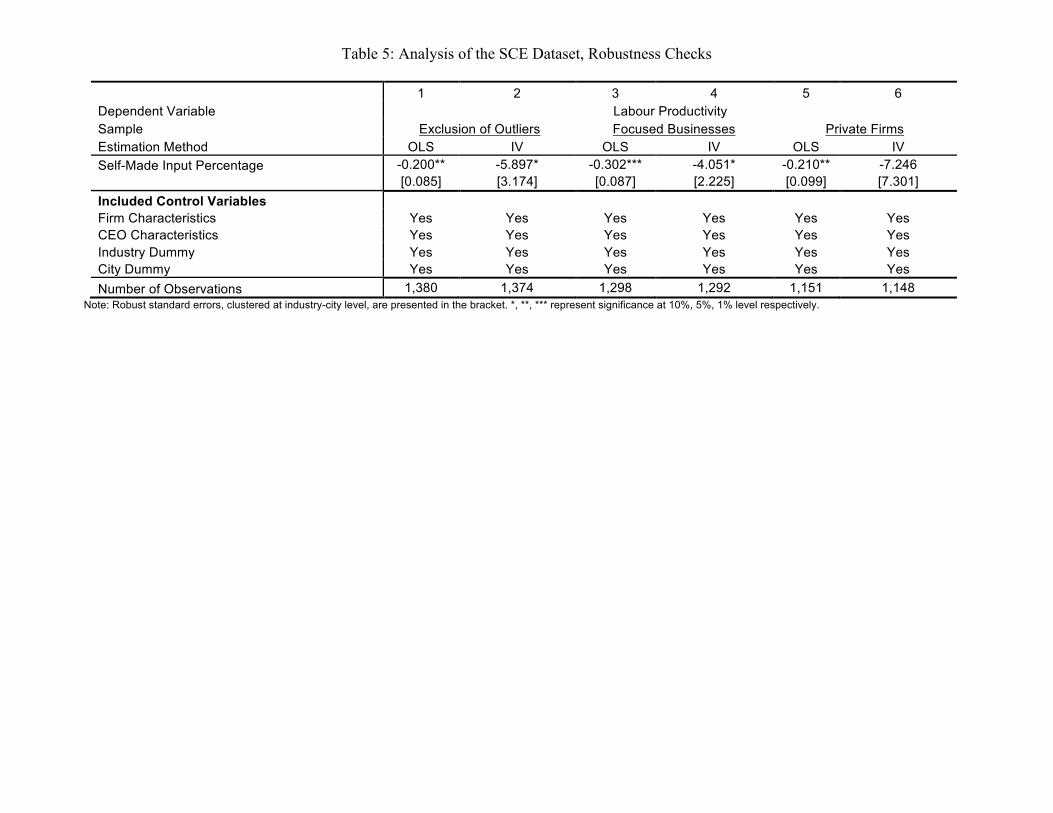
Table 5: Analysis of the SCE Dataset, Robustness Checks

1 2 3 4 5 6 Dependent Variable Labour Productivity Sample Exclusion of Outliers Focused Businesses Private Firms Estimation Method OLS IV OLS IV OLS IV Self-Made Input Percentage -0.200** -5.897* -0.302*** -4.051* -0.210** -7.246 [0.085] [3.174] [0.087] [2.225] [0.099] [7.301] Included Control Variables Firm Characteristics Yes Yes Yes Yes Yes Yes CEO Characteristics Yes Yes Yes Yes Yes Yes Industry Dummy Yes Yes Yes Yes Yes Yes City Dummy Yes Yes Yes Yes Yes Yes Number of Observations 1,380 1,374 1,298 1,292 1,151 1,148

Note: Robust standard errors, clustered at industry-city level, are presented in the bracket. *, **, *** represent significance at 10%, 5%, 1% level respectively.

Table 6: Analysis of the ASIF Dataset, Main Results

1 2 3 4 Dependent Variable Labour Productivity

Estimation Pooled OLS Panel Fixed-Effect Panel Fixed-Effect Anderson-Hsiao IV Panel A: Contemporary Effects Value Added Ratio -1.274*** -0.627*** -0.552*** -0.470*** [0.011] [0.008] [0.009] [0.015] Lagged Labour Productivity 0.176*** 0.286*** [0.003] [0.007] Number of Observations 943,257 943,257 634,141 398,380 Panel B: One-Year Lagged Effects Value Added Ratio -1.061*** -0.549*** -0.523*** -0.369*** [0.012] [0.010] [0.010] [0.018] Lagged (1y) Value Added Ratio -0.494*** -0.108*** -0.013* 0.104*** [0.010] [0.008] [0.008] [0.010] Lagged Labour Productivity 0.172*** 0.318*** [0.003] [0.008] Number of Observations 614,697 614,697 567,524 360,405 Panel C: Two-Year Lagged Effects Value Added Ratio -0.982*** -0.520*** -0.501*** -0.352*** [0.016] [0.013] [0.012] [0.029] Lagged (1y) Value Added Ratio -0.404*** -0.102*** -0.030*** 0.117*** [0.014] [0.011] [0.010] [0.017] Lagged (2y) Value Added Ratio -0.349*** -0.041*** -0.031*** 0.004 [0.014] [0.010] [0.009] [0.011] Lagged Labour Productivity 0.150*** 0.399*** [0.005] [0.013] Number of Observations 362,045 362,045 360,795 223,174 Year Dummy Yes Yes Yes Yes Industry Dummy Yes Province Dummy Yes Firm Dummy Yes Yes Yes

Note: Robust standard errors, clustered at firm level, are presented in the bracket. *, **, *** represent significance at 10%, 5%, 1% level respectively.

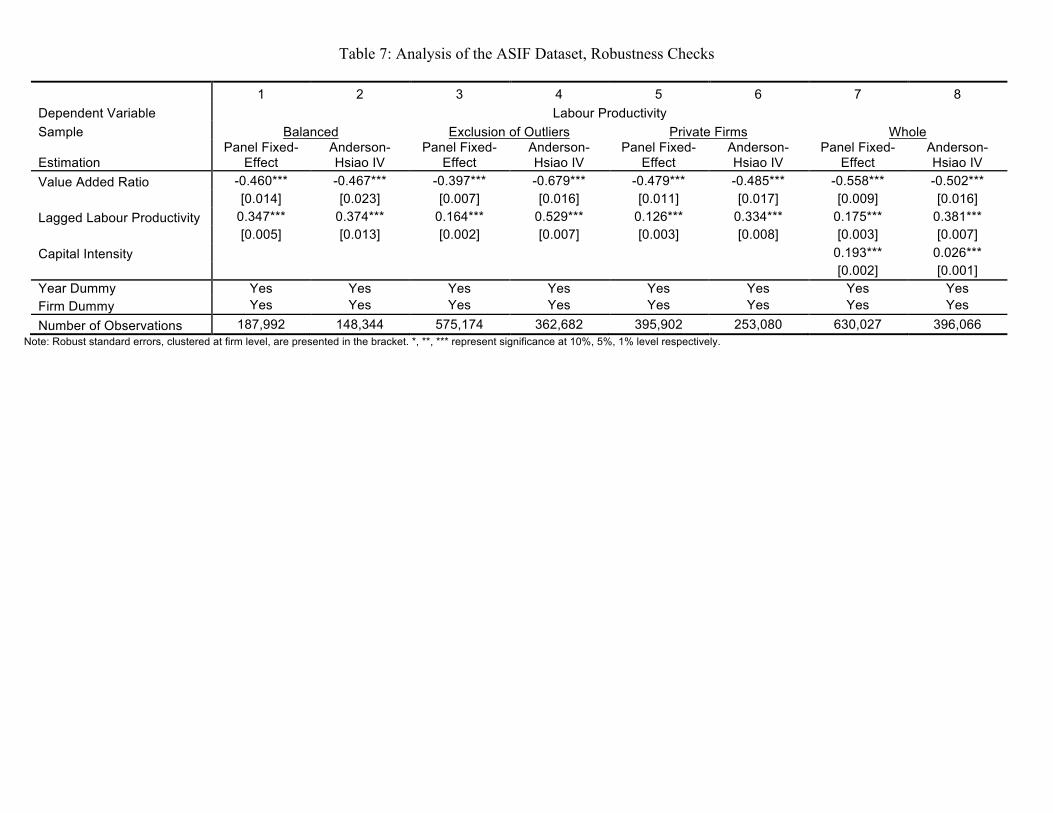
Table 7: Analysis of the ASIF Dataset, Robustness Checks

1 2 3 4 5 6 7 8 Dependent Variable Labour Productivity Sample Balanced Exclusion of Outliers Private Firms Whole

Estimation Panel Fixed-

Effect Anderson-Hsiao IV

Panel Fixed-Effect

Anderson-Hsiao IV

Panel Fixed-Effect

Anderson-Hsiao IV

Panel Fixed-Effect

Anderson-Hsiao IV

Value Added Ratio -0.460*** -0.467*** -0.397*** -0.679*** -0.479*** -0.485*** -0.558*** -0.502*** [0.014] [0.023] [0.007] [0.016] [0.011] [0.017] [0.009] [0.016] Lagged Labour Productivity 0.347*** 0.374*** 0.164*** 0.529*** 0.126*** 0.334*** 0.175*** 0.381*** [0.005] [0.013] [0.002] [0.007] [0.003] [0.008] [0.003] [0.007] Capital Intensity 0.193*** 0.026*** [0.002] [0.001] Year Dummy Yes Yes Yes Yes Yes Yes Yes Yes Firm Dummy Yes Yes Yes Yes Yes Yes Yes Yes Number of Observations 187,992 148,344 575,174 362,682 395,902 253,080 630,027 396,066

Note: Robust standard errors, clustered at firm level, are presented in the bracket. *, **, *** represent significance at 10%, 5%, 1% level respectively.

Table 8: Analysis of the PESPIC Dataset, Main Results

1 2 3 4 5 6 Dependent Variable Change in Labour Productivity Change in Vertical Integration -0.091** -0.095** -0.095** -0.095** -0.092** -0.076** [0.036] [0.037] [0.037] [0.037] [0.036] [0.037] Initial Firm Size 0.085*** 0.084*** 0.084*** 0.085*** 0.085*** 0.076*** [0.026] [0.026] [0.026] [0.026] [0.026] [0.025] Initial Sales Change 0.027*** 0.026*** 0.027*** 0.027*** 0.027*** 0.017** [0.008] [0.008] [0.009] [0.009] [0.009] [0.008] Introduction of New Technology 0.018 0.019 0.018 0.022 0.005 [0.028] [0.028] [0.028] [0.029] [0.029] Introduction of New Joint Venture -0.024 -0.029 -0.027 0.014 [0.058] [0.064] [0.064] [0.056] Introduction of New Licensing Agreement 0.016 0.018 -0.003 [0.054] [0.054] [0.052] Introduction of New Major Product Line -0.018 -0.002 [0.027] [0.026] Change in Capital Intensity 0.258*** [0.045] Number of Observations 2,672 2,671 2,670 2,670 2,670 2,583

Note: Robust standard errors, clustered at firm level, are presented in the bracket. *, **, *** represent significance at 10%, 5%, 1% level respectively.

Table 9: Analysis of the PESPIC Dataset, Robustness Checks

1 2 Dependent Variable Change in Labour Productivity Sample Exclusion of Outlying Observations Private Firms Change in Vertical Integration -0.057*** -0.090** [0.021] [0.036] Initial Firm Size 0.084*** 0.085*** [0.022] [0.026] Initial Sales Change 0.035*** 0.026*** [0.006] [0.008] Number of Observations 2,637 2,658

Note: Robust standard errors, clustered at firm level, are presented in the bracket. *, **, *** represent significance at 10%, 5%, 1% level respectively.