Verifying Ray Tracing Based CoMP–MIMOPredictions with Channel Sounding Measurements

Richard Fritzsche1, Jens Voigt2, Carsten Jandura1, and Gerhard P. Fettweis1

1Dresden University of Technology, Vodafone Chair for Mobile Commnications Sytems, Dresden, Germany2Actix GmbH, Dresden, Germany, jens.voigt@actix.com

{richard.fritzsche, carsten.jandura, fettweis}@ifn.et.tu-dresden.de

Abstract— Multiple-Input Multiple–Output (MIMO) technol-ogy is ready for deployment in commercial cellular networksin the very near future. Thus, the need of incorporating thistechnology into radio network planning and optimization risesdramatically for network operators. The main question to an-swer is how accurate MIMO channel models reflect the realMIMO channel. In this contribution we verify a detailed raytracing channel simulator with channel sounding measurementsin the 2.53 GHz range by comparing simulated and measuredeigenvalue characteristics for various Single–User (SU) downlinkscenarios in a Coordinated Multi–Point (CoMP) environment.From our comparison we can conclude that carefully performedGeometrical Optics based ray tracing simulations are an ade-quate prediction model to reflect main characteristics of SU–MIMO channels even in a CoMP scenario.

I. INTRODUCTION

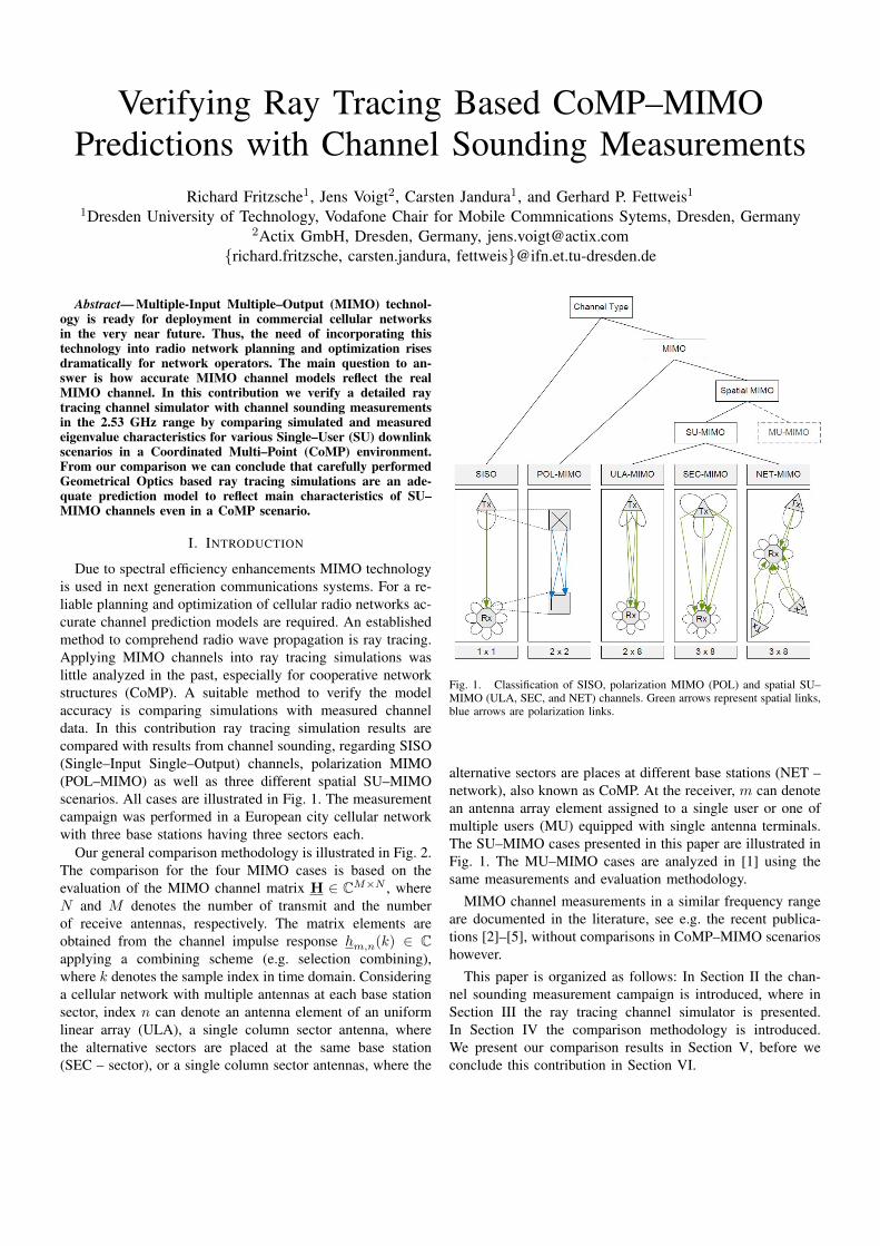
Due to spectral efficiency enhancements MIMO technologyis used in next generation communications systems. For a re-liable planning and optimization of cellular radio networks ac-curate channel prediction models are required. An establishedmethod to comprehend radio wave propagation is ray tracing.Applying MIMO channels into ray tracing simulations waslittle analyzed in the past, especially for cooperative networkstructures (CoMP). A suitable method to verify the modelaccuracy is comparing simulations with measured channeldata. In this contribution ray tracing simulation results arecompared with results from channel sounding, regarding SISO(Single–Input Single–Output) channels, polarization MIMO(POL–MIMO) as well as three different spatial SU–MIMOscenarios. All cases are illustrated in Fig. 1. The measurementcampaign was performed in a European city cellular networkwith three base stations having three sectors each.

Our general comparison methodology is illustrated in Fig. 2.The comparison for the four MIMO cases is based on theevaluation of the MIMO channel matrix H ∈ CM×N , whereN and M denotes the number of transmit and the numberof receive antennas, respectively. The matrix elements areobtained from the channel impulse response hm,n(k) ∈ Capplying a combining scheme (e.g. selection combining),where k denotes the sample index in time domain. Consideringa cellular network with multiple antennas at each base stationsector, index n can denote an antenna element of an uniformlinear array (ULA), a single column sector antenna, wherethe alternative sectors are placed at the same base station(SEC – sector), or a single column sector antennas, where the

Fig. 1. Classification of SISO, polarization MIMO (POL) and spatial SU–MIMO (ULA, SEC, and NET) channels. Green arrows represent spatial links,blue arrows are polarization links.

alternative sectors are places at different base stations (NET –network), also known as CoMP. At the receiver, m can denotean antenna array element assigned to a single user or one ofmultiple users (MU) equipped with single antenna terminals.The SU–MIMO cases presented in this paper are illustrated inFig. 1. The MU–MIMO cases are analyzed in [1] using thesame measurements and evaluation methodology.

MIMO channel measurements in a similar frequency rangeare documented in the literature, see e.g. the recent publica-tions [2]–[5], without comparisons in CoMP–MIMO scenarioshowever.

This paper is organized as follows: In Section II the chan-nel sounding measurement campaign is introduced, where inSection III the ray tracing channel simulator is presented.In Section IV the comparison methodology is introduced.We present our comparison results in Section V, before weconclude this contribution in Section VI.

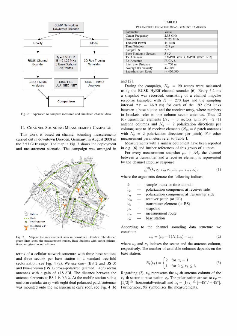
Fig. 2. Approach to compare measured and simulated channel data.

II. CHANNEL SOUNDING MEASUREMENT CAMPAIGN

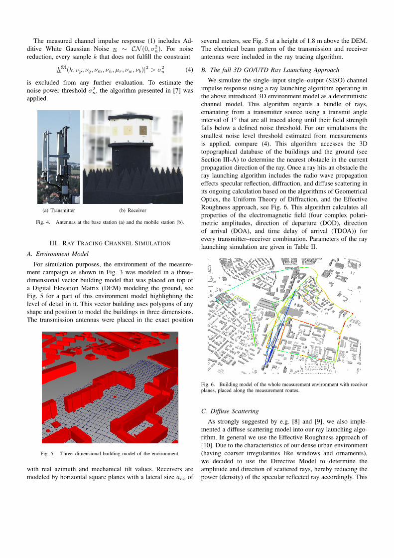
This work is based on channel sounding measurementscarried out in downtown Dresden, Germany, in August 2008 inthe 2.53 GHz range. The map in Fig. 3 shows the deploymentand measurement scenario. The campaign was arranged in

Fig. 3. Map of the measurement area in downtown Dresden. The dashedgreen lines show the measurement routes. Base Stations with sector orienta-tions are given as red ellipses.

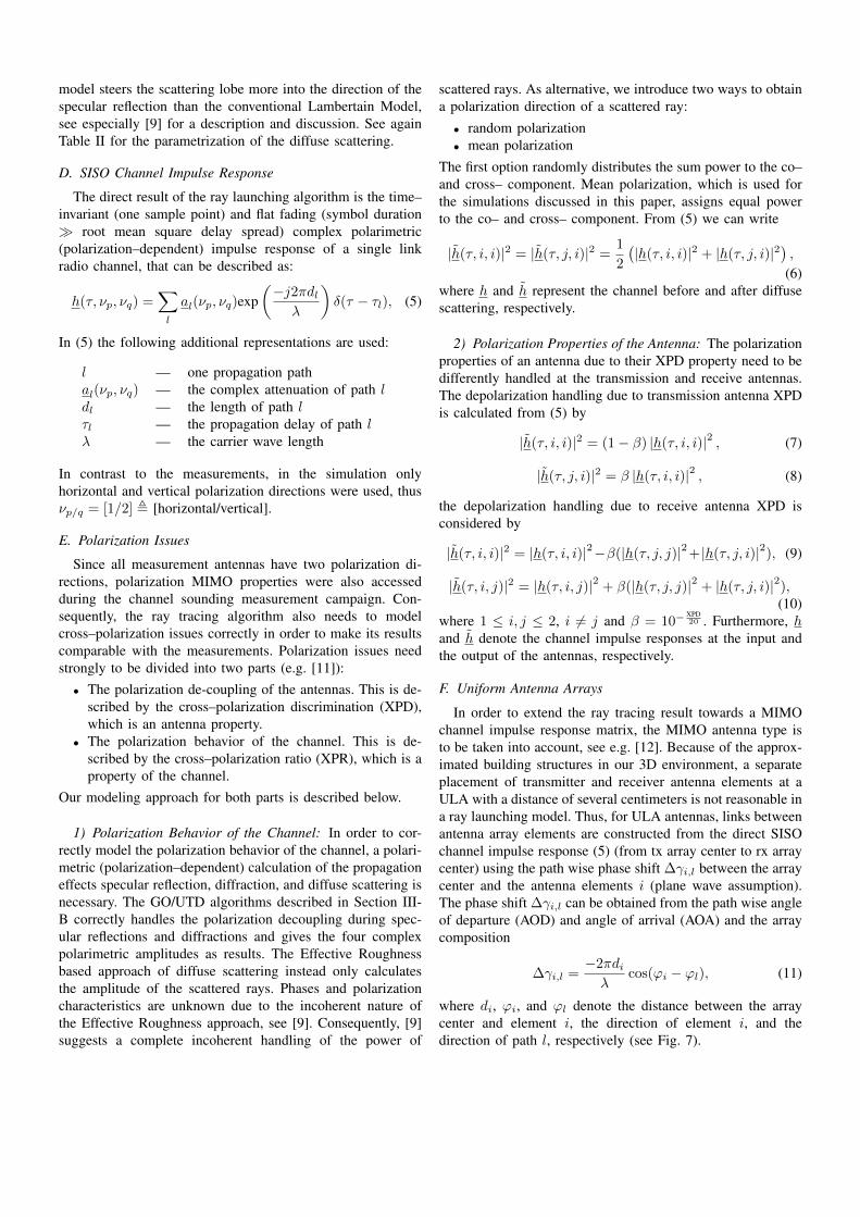
terms of a cellular network structure with three base stationsand three sectors per base station in a standard tree-foldsectorization, see Fig. 4 (a). We use one– (BS 2 and BS 3)and two–column (BS 1) cross–polarized (slanted ±45◦) sectorantennas with a gain of +18 dBi. The distance between theantenna elements at BS 1 is 0.6 λ. At the mobile station side auniform circular array with eight dual polarized patch antennaswas mounted onto the measurement car’s roof, see Fig. 4 (b)

TABLE IPARAMETERS FROM THE MEASUREMENT CAMPAIGN

Parameter ValueCenter Frequency 2.53 GHzBandwidth 21.25 MHzTransmit Power 44 dBmTime Window 12.8 µsSamples K 273Base Stations / Sectors 3 / 3Tx Antennas XX-POL (BS1), X-POL (BS2, BS3)Rx Antennas PUCA 8Inter Site Distance ≈ 750 mAverage Rx Velocity 4.2 m/sSnapshots per Route ≈ 450.000

and [2].During the campaign, Nw = 29 routes were measured

using the RUSK HyEff channel sounder [6]. Every 5.2 msa snapshot was recorded, consisting of a channel impulseresponse (sampled with K = 273 taps and the samplinginterval ∆τ = 46.9 ns) for each of the 192 (96) linksbetween a base station and the receiver array, where numbersin brackets refer to one–column sector antennas. Thus 12(6) transmitter elements (Ns = 3 sectors with Nt =2 (1)antenna columns and Nq = 2 polarization directions percolumn) sent to 16 receiver elements (Nm = 8 patch antennaswith Np = 2 polarization directions per patch). For othermeasurement parameters refer to Table I.

Measurements with a similar equipment have been reportedin e.g. [6] and further references of this group of authors.

For every measurement snapshot µr ∈ Mr the channelbetween a transmitter and a receiver element is representedby the channel impulse response

hM(k, νp, νq, νm, νn, µr, νw, νb), (1)

where the arguments denote the following indices:

k — sample index in time domainνp — polarization component at receiver sideνq — polarization component at transmitter sideνm — receiver patch (at UE)νn — transmitter element (at BS)µr — snapshotνw — measurement routeνb — base station

According to the channel sounding data structure weconstitute

νn = (νs − 1)Nt(νb) + νt, (2)

where νs and νt indexes the sector and the antenna column,respectively. The number of available columns depends on thebase station:

Nt(νb) =

{2 for νb = 1

1 for 2 ≤ νb ≤ 3(3)

Regarding (2), νn represents the νt-th antenna column of theνs-th sector at base station νb. The polarization are set to νp =[1/2] , [horizontal/vertical] and νq = [1/2] , [−45◦/+ 45◦].Furthermore, M symbolizes the measurements.

The measured channel impulse response (1) includes Ad-ditive White Gaussian Noise n ∼ CN (0, σ2

n). For noisereduction, every sample k that does not fulfill the constraint

|hM(k, νp, νq, νm, νn, µr, νw, νb)|2 > σ2n (4)

is excluded from any further evaluation. To estimate thenoise power threshold σ2

n, the algorithm presented in [7] wasapplied.

(a) Transmitter (b) Receiver

Fig. 4. Antennas at the base station (a) and the mobile station (b).

III. RAY TRACING CHANNEL SIMULATION

A. Environment Model

For simulation purposes, the environment of the measure-ment campaign as shown in Fig. 3 was modeled in a three–dimensional vector building model that was placed on top ofa Digital Elevation Matrix (DEM) modeling the ground, seeFig. 5 for a part of this environment model highlighting thelevel of detail in it. This vector building uses polygons of anyshape and position to model the buildings in three dimensions.The transmission antennas were placed in the exact position

Fig. 5. Three–dimensional building model of the environment.

with real azimuth and mechanical tilt values. Receivers aremodeled by horizontal square planes with a lateral size arx of

several meters, see Fig. 5 at a height of 1.8 m above the DEM.The electrical beam pattern of the transmission and receiverantennas were included in the ray tracing algorithm.

B. The full 3D GO/UTD Ray Launching Approach

We simulate the single–input single–output (SISO) channelimpulse response using a ray launching algorithm operating inthe above introduced 3D environment model as a deterministicchannel model. This algorithm regards a bundle of rays,emanating from a transmitter source using a transmit angleinterval of 1◦ that are all traced along until their field strengthfalls below a defined noise threshold. For our simulations thesmallest noise level threshold estimated from measurementsis applied, compare (4). This algorithm accesses the 3Dtopographical database of the buildings and the ground (seeSection III-A) to determine the nearest obstacle in the currentpropagation direction of the ray. Once a ray hits an obstacle theray launching algorithm includes the radio wave propagationeffects specular reflection, diffraction, and diffuse scattering inits ongoing calculation based on the algorithms of GeometricalOptics, the Uniform Theory of Diffraction, and the EffectiveRoughness approach, see Fig. 6. This algorithm calculates allproperties of the electromagnetic field (four complex polari-metric amplitudes, direction of departure (DOD), directionof arrival (DOA), and time delay of arrival (TDOA)) forevery transmitter–receiver combination. Parameters of the raylaunching simulation are given in Table II.

Fig. 6. Building model of the whole measurement environment with receiverplanes, placed along the measurement routes.

C. Diffuse Scattering

As strongly suggested by e.g. [8] and [9], we also imple-mented a diffuse scattering model into our ray launching algo-rithm. In general we use the Effective Roughness approach of[10]. Due to the characteristics of our dense urban environment(having coarser irregularities like windows and ornaments),we decided to use the Directive Model to determine theamplitude and direction of scattered rays, hereby reducing thepower (density) of the specular reflected ray accordingly. This

model steers the scattering lobe more into the direction of thespecular reflection than the conventional Lambertain Model,see especially [9] for a description and discussion. See againTable II for the parametrization of the diffuse scattering.

D. SISO Channel Impulse Response

The direct result of the ray launching algorithm is the time–invariant (one sample point) and flat fading (symbol duration� root mean square delay spread) complex polarimetric(polarization–dependent) impulse response of a single linkradio channel, that can be described as:

h(τ, νp, νq) =∑l

al(νp, νq)exp(−j2πdlλ

)δ(τ − τl), (5)

In (5) the following additional representations are used:

l — one propagation pathal(νp, νq) — the complex attenuation of path ldl — the length of path lτl — the propagation delay of path lλ — the carrier wave length

In contrast to the measurements, in the simulation onlyhorizontal and vertical polarization directions were used, thusνp/q = [1/2] , [horizontal/vertical].

E. Polarization Issues

Since all measurement antennas have two polarization di-rections, polarization MIMO properties were also accessedduring the channel sounding measurement campaign. Con-sequently, the ray tracing algorithm also needs to modelcross–polarization issues correctly in order to make its resultscomparable with the measurements. Polarization issues needstrongly to be divided into two parts (e.g. [11]):• The polarization de-coupling of the antennas. This is de-

scribed by the cross–polarization discrimination (XPD),which is an antenna property.

• The polarization behavior of the channel. This is de-scribed by the cross–polarization ratio (XPR), which is aproperty of the channel.

Our modeling approach for both parts is described below.

1) Polarization Behavior of the Channel: In order to cor-rectly model the polarization behavior of the channel, a polari-metric (polarization–dependent) calculation of the propagationeffects specular reflection, diffraction, and diffuse scattering isnecessary. The GO/UTD algorithms described in Section III-B correctly handles the polarization decoupling during spec-ular reflections and diffractions and gives the four complexpolarimetric amplitudes as results. The Effective Roughnessbased approach of diffuse scattering instead only calculatesthe amplitude of the scattered rays. Phases and polarizationcharacteristics are unknown due to the incoherent nature ofthe Effective Roughness approach, see [9]. Consequently, [9]suggests a complete incoherent handling of the power of

scattered rays. As alternative, we introduce two ways to obtaina polarization direction of a scattered ray:• random polarization• mean polarization

The first option randomly distributes the sum power to the co–and cross– component. Mean polarization, which is used forthe simulations discussed in this paper, assigns equal powerto the co– and cross– component. From (5) we can write

|h(τ, i, i)|2 = |h(τ, j, i)|2 =1

2

(|h(τ, i, i)|2 + |h(τ, j, i)|2

),

(6)where h and h represent the channel before and after diffusescattering, respectively.

2) Polarization Properties of the Antenna: The polarizationproperties of an antenna due to their XPD property need to bedifferently handled at the transmission and receive antennas.The depolarization handling due to transmission antenna XPDis calculated from (5) by

|h(τ, i, i)|2 = (1− β) |h(τ, i, i)|2 , (7)

|h(τ, j, i)|2 = β |h(τ, i, i)|2 , (8)

the depolarization handling due to receive antenna XPD isconsidered by

|h(τ, i, i)|2 = |h(τ, i, i)|2−β(|h(τ, j, j)|2 +|h(τ, j, i)|2), (9)

|h(τ, i, j)|2 = |h(τ, i, j)|2 + β(|h(τ, j, j)|2 + |h(τ, j, i)|2),(10)

where 1 ≤ i, j ≤ 2, i 6= j and β = 10−XPD20 . Furthermore, h

and h denote the channel impulse responses at the input andthe output of the antennas, respectively.

F. Uniform Antenna Arrays

In order to extend the ray tracing result towards a MIMOchannel impulse response matrix, the MIMO antenna type isto be taken into account, see e.g. [12]. Because of the approx-imated building structures in our 3D environment, a separateplacement of transmitter and receiver antenna elements at aULA with a distance of several centimeters is not reasonable ina ray launching model. Thus, for ULA antennas, links betweenantenna array elements are constructed from the direct SISOchannel impulse response (5) (from tx array center to rx arraycenter) using the path wise phase shift ∆γi,l between the arraycenter and the antenna elements i (plane wave assumption).The phase shift ∆γi,l can be obtained from the path wise angleof departure (AOD) and angle of arrival (AOA) and the arraycomposition

∆γi,l =−2πdiλ

cos(ϕi − ϕl), (11)

where di, ϕi, and ϕl denote the distance between the arraycenter and element i, the direction of element i, and thedirection of path l, respectively (see Fig. 7).

Fig. 7. Calculation of the path wise phase shift at the array element i.

From (12) a generic channel impulse response consideringa uniform array at transmitter and receiver can be written as:

h(τ, νp, νq, νm, νn) =∑l

al(νp, νq)δ (τ − τl) · ...

ψνm,l · e(−j 2πdl

λ +∆γrxνm,l+∆γtxνt,l),

(12)

where the transmitter elements are indexed by

νn = (νs − 1)Nt(νb) + νt, (13)

according to the notation from Section II.Note that we model magnitude variations between array

elements at the receiver, e.g. due to fading effects, withthe random variable ψνm,l ∼ N (1, σ2

a), where σ2a denotes

the variance of the magnitude of a in order to lower thecorrelations between the ULA antenna elements further thanthe phase shift of the plane wave model. Notice that ψνm,l isonly considered in the ULA scenario. Otherwise we constituteψνm,l = 1.

Furthermore, we sample the channel impulse response ob-tained from (12) to

h(k, νp, νq, νm, νn) =

∫ k∆τ

(k−1)∆τ

h(τ, νp, νq, νm, νn)dτ. (14)

For the discussions in Section IV the channel impulse responseis written depending on the receiver plane νr, the measurementroute νw and the base station νb, compare to (1)

hS(k, νp, νq, νm, νn, νr, νw, νb), (15)

where S represents the simulation.

TABLE IIPARAMETERS FOR THE RAY LAUNCHING ALGORITHM

Parameter ValueCenter Frequency 2.53 GHzRelative Permittivity, real part 4.0Effective Roughness [8], [9] 0.3Scattering Directivity [8], [9] 4.0Transmit Angle Interval 1◦

Max. Number of Reflections per Ray ∞Max. Number of Diffractions per Ray 2

IV. COMPARISON METHODOLOGY

In this section we describe the mathematical approachto map the ray tracing simulation results and the channelsounding measurements to each other in order to be able tocompare them.

A. Position Mapping

As mentioned in Section III a receiver plane in the raytracing simulation has a lateral size of arx = 10 m. Duringthe channel sounding measurements, the car’s speed was about4.2 m/s (see Table I), while a snapshot was taken every 5.2 ms.This leads to about 450 measurement snapshots per simulatedreceiver plane. Based on geographical snapshot information(xµr , yµr , zµr ) a set M(νr) including the indices of allsnapshots lying inside the receiver plane νr is introduced

M(νr) = {µr|xζ(νr−1)+1 ≤ xµr ≤ dx(νr − 1)arx,

yζ(νr−1)+1 ≤ yµr ≤ dy(νr − 1)arx},(16)

where the instantaneous route direction is formulated as

dx(νr) = sgn(xζ(νr) − xζ(νr−1)+1), (17)

dy(νr) = sgn(yζ(νr) − yζ(νr−1)+1). (18)

The function ζ maps the last element of M(νr) to νr

ζ(νr) =

0 for νr = 0

maxµr∈M(νr)

µr for 1 ≤ νr ≤ Nr (19)

The mapping procedure is illustrated in Fig. 8. By calculatingM(1) the first snapshots of a route are mapped to the firstreceiver. The final receiver position is got from the averageof the related snapshot positions. The procedure is applieduntil all snapshots of a route are mapped to receivers. At the

Fig. 8. Illustration of the mapping function ζ.

simulation a receiver νr collects each wave front hitting itsplane. FromM(νr) we want to find the snapshot that receivedthe most dominant of these wave fronts. Hence, we select thesnapshot with the highest power. Based on (1) and (15) aselection function can be written as follows:

µr(νr) = argmaxµr∈M(νr)

∑νm

∑νn

pM(νm, νn, µr) (20)

with

pM/S(νm, νn, µr) =∑k

∑νp

∑νq

|hM/S(k, νp, νq, νm, νn, µr)|2,

(21)where we disclaim to explicitly note the arguments νw and νb.

B. SISO Channel Property Analysis

We compare the pathloss between the ray tracing simulationand the channel sounding measurements as the main SISOchannel property. For this comparison the antenna element νmof the receiver array νr with the highest receive power duringthe measurements is chosen:

νm(νr) = argmax1≤νm≤Nm

∑νn

pM(νm, νn, µr(νr)). (22)

The pathloss is calculated out of the measurement results byselecting the patch νm at the receiver and the antenna elementνn(νs, νb) at the transmitter, where we appoint νt = 1 (selectsalways the first column of a two column sector antenna) from(21):

LM(νr) = 10 log10

(pM(νm, νn, µr(νr))

). (23)

The pathloss from simulation results is obtained again from(21) by

LS(νr) = 10 log10

(pS(νm, νn, νr)

). (24)

C. MIMO Channel Property Analysis

The quality of the MIMO channel can be described by theMIMO channel capacity. For an equal power distribution forall antenna elements at the transmitter side the capacity in theWhite Gaussian Noise channel can be calculated by

C =

rH∑i=1

log2

(1 +

σ2S

σ2N

λi

), (25)

where rH is the rank of H and λi are the eigenvalues ofH HH . The ratio of signal power σ2

S to noise power σ2N is

called Signal–to–Noise–Ratio (SNR). To obtain independencefrom SNR only the distribution of the normalized eigenvaluesare considered for the following analysis, compare e.g. [13]. Inthis contribution MIMO systems with a maximum rank rH ≤3 are used. Because in this case the smallest eigenvalue isusually negligible in reality, we assume that the considerationof the two strongest eigenvalues is sufficient. As a reasonablestatistic to describe the MIMO channel structure we introducethe eigenvalue ratio:

reig = 10 log10

maxj=1,...,rH |j 6=i

(λj)

maxi=1,...,rH

(λi)

, (26)

where the second best eigenvalue is divided by the besteigenvalue. We now give the formulas to calculate the elementsof the channel impulse response matrices for the simulationand measurement case for all four MIMO setups (compareFig. 1) that we used for our comparison:• polarization MIMO (POL–MIMO),• spatial MIMO with a ULA at transmitter (ULA–MIMO),• cooperation of different sectors at the same site (SEC–

MIMO),• cooperation of sectors at different sites (NET–MIMO).

Then, a respective channel matrix is constructed for everysetup and used to calculate the eigenvalues and their ratio

for later comparison. Thereby the channel impulse responseof a link has to be reduced to a single channel coefficient. Weconsidered selection combining (selection of the sample withthe highest power).

1) POL–MIMO: The elements of the polarization MIMOchannel impulse response matrix HPOL ∈ C2×2 for themeasurements are obtained from (1) by

hPOL,Mi,j (k, νr, νw, νb) = hM(k, i, j, νm, νn, µr(νr), νw, νb).

(27)Since the measurement transmit antennas use different polar-ization directions than the respective antennas in the simulationcase, the ±45◦ polarization at measurement transmit antennasis shifted back to horizontal/vertical polarization (like thetransmit antennas at the simulation) using the rotation matrix

T =1√2

[1 1−1 1

](28)

and calculating

HPOL,M = HPOL,M

T. (29)

The elements of the polarization MIMO channel impulseresponse matrix for the simulation are obtained from (15) by

hPOL,Si,j (k, νr, νw, νb) = hS(k, i, j, νm, νn, νr, νw, νb). (30)

2) Spatial MIMO: For the three spatial MIMO cases areduced channel impulse response is used, where one polar-ization component is selected at the transmitter (νq = 1) andthe both resulting polarization components at the receiver areadded. From the matrix elements of (29) and from (30) weget

hM/S

(k, νm, νn, νr, νw, νb) =∑i

hPOL,M/Si,1 (k, νm, νn, νr, νw, νb),

(31)

taking νm and νn into account.

a) ULA–MIMO: Based on (31) the coefficients of thechannel impulse response matrix for the ULA case HULA ∈C8×2 are selected by

hULA,Mi,j (k, νr, νw, νs) = h

M(k, i, νn(j, νs), µr(νr), νw, 1)

(32)from measurement results and by

hULA,Si,j (k, νr, νw, νs) = h

S(k, i, νn(j, νs), νr, νw, 1) (33)

from simulation results. Because BS 1 is the only base stationusing two–column sector antennas, it is the only one used forULA analysis.

b) SEC–MIMO: The elements of the channel impulseresponse matrix for SEC–MIMO HSEC ∈ C8×3 are obtainedby

hSEC,Mi,j (k, νr, νw, νb) = h

M(k, i, νn(νb, j), µr(νr), νw, νb)

(34)

from measurement results and by

hSEC,Si,j (k, νr, νw, νb) = h

S(k, i, νn(νb, j), νr, νw, νb) (35)

from simulation results, both from (31). We obtain the selectedtransmitter elements by

νn(νb, j) = (j − 1)Nt(νb) + 1. (36)

Remember, as mentioned in Section II, Nt = 2 for BS 1 andNt = 1 for BS 2 and BS 3. In the case of SEC–MIMO onlyone column of the two–column antennas at BS 1 is used foranalysis.

c) NET–MIMO: The elements of the channel impulseresponse matrix for NET–MIMO HNET ∈ C8×3 are obtainedby

hNET,Mi,j (k, νr, νw, νs, νb) =

hM

(k, i, νn(νs, νb, j), µr(νr), νw, νb) (37)

for the measured channel and by

hNET,Si,j (k, νr, νw, νs, νb) = h

S(k, i, νn(νs, νb, j), νr, νw, νb)

(38)for the simulated channel, both again from (31). The transmit-ter elements are taken from

νn(νs, νb, j) = (νs − 1)Nt(νb) + 1. (39)

Obviously not every combination of sectors and base stationsis reasonable. Hence, preselections of sectors that cover thesame area were done.

V. RESULTS

A. SISO Analysis

The cumulative distribution function (CDF) of the simulatedpathloss (24) is compared to the CDF of the measured pathloss(23) on the left side of Fig. 9. The point-by-point deviation be-tween simulation and measurement results (∆L = LS−LM)is shown on the right side of Fig. 9. The results indicate thatfor 75% of the analyzed receiver positions in our environmentthe pathloss deviation between simulation and measurement isless than 10 dB. The average value of the difference is 0.11 dB.

B. MIMO Analysis

1) Polarization MIMO: For POL–MIMO the channel im-pulse response matrices are given in (30) for simulationdata and in (27) for measurement data. The result of theeigenvalue difference is shown in Fig. 10. The separationof the results into line–of–sight (LoS) and non–line–of–sight(NLoS) situations illustrates a better fitting for NLoS scenar-ios. The difference for LoS is considerably smaller when theXPD properties of the transmission and receive antennas arecorrectly handled in the ray tracing simulation, see Section III-E.2. Enabling the diffuse scattering option in the ray tracingsimulation results in negligible differences in the eigenvalueratio deviation for POL–MIMO only, compare Fig. 11.

Fig. 9. Comparison of the pathloss and its deviations between measurementsand simulation.

Fig. 10. Comparison of the eigenvalue ratio for measurements and simulationfor POL–MIMO.

Fig. 11. Eigenvalue ratio deviation for POL–MIMO with and without DiffuseScattering option in the simulation.

2) Spatial MIMO: For the three different spatial MIMO se-tups ULA–MIMO, SEC–MIMO, and NET–MIMO the channelimpulse matrices for simulation and measurements are givenin (32) to (38). As can clearly be seen from Fig. 12, for

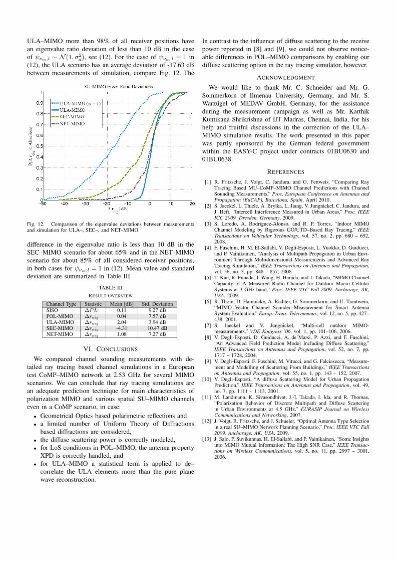
ULA–MIMO more than 98% of all receiver positions havean eigenvalue ratio deviation of less than 10 dB in the caseof ψνm,l ∼ N (1, σ2

a), see (12). For the case of ψνm,l = 1 in(12), the ULA scenario has an average deviation of -17.63 dBbetween measurements of simulation, compare Fig. 12. The

Fig. 12. Comparison of the eigenvalue deviations between measurementsand simulation for ULA–, SEC–, and NET–MIMO.

difference in the eigenvalue ratio is less than 10 dB in theSEC–MIMO scenario for about 65% and in the NET–MIMOscenario for about 85% of all considered receiver positions,in both cases for ψνm,l = 1 in (12). Mean value and standarddeviation are summarized in Table III.

TABLE IIIRESULT OVERVIEW

Channel Type Statistic Mean [dB] Std. DeviationSISO ∆PL 0.11 9.27 dBPOL-MIMO ∆reig 0.04 7.57 dBULA-MIMO ∆reig 2.04 3.94 dBSEC-MIMO ∆reig -4.31 10.47 dBNET-MIMO ∆reig 1.08 7.27 dB

VI. CONCLUSIONS

We compared channel sounding measurements with de-tailed ray tracing based channel simulations in a Europeantest CoMP–MIMO network at 2.53 GHz for several MIMOscenarios. We can conclude that ray tracing simulations arean adequate prediction technique for main characteristics ofpolarization MIMO and various spatial SU–MIMO channelseven in a CoMP scenario, in case:• Geometrical Optics based polarimetric reflections and• a limited number of Uniform Theory of Diffractions

based diffractions are considered,• the diffuse scattering power is correctly modeled,• for LoS conditions in POL–MIMO, the antenna property

XPD is correctly handled, and• for ULA–MIMO a statistical term is applied to de–

correlate the ULA elements more than the pure planewave reconstruction.

In contrast to the influence of diffuse scattering to the receivepower reported in [8] and [9], we could not observe notice-able differences in POL–MIMO comparisons by enabling ourdiffuse scattering option in the ray tracing simulator, however.

ACKNOWLEDGMENT

We would like to thank Mr. C. Schneider and Mr. G.Sommerkorn of Ilmenau University, Germany, and Mr. S.Warzugel of MEDAV GmbH, Germany, for the assistanceduring the measurement campaign as well as Mr. KarthikKuntikana Shrikrishna of IIT Madras, Chennai, India, for hishelp and fruitful discussions in the correction of the ULA–MIMO simulation results. The work presented in this paperwas partly sponsored by the German federal governmentwithin the EASY-C project under contracts 01BU0630 and01BU0638.

REFERENCES

[1] R. Fritzsche, J. Voigt, C. Jandura, and G. Fettweis, “Comparing RayTracing Based MU–CoMP–MIMO Channel Predictions with ChannelSounding Measurements,” Proc. European Conference on Antennas andPropagation (EuCAP), Barcelona, Spain, April 2010.

[2] S. Jaeckel, L. Thiele, A. Brylka, L. Jiang, V. Jungnickel, C. Jandura, andJ. Heft, “Intercell Interference Measured in Urban Areas,” Proc. IEEEICC 2009, Dresden, Germany, 2009.

[3] S. Loredo, A. Rodriguez-Alonso, and R. P. Torres, “Indoor MIMOChannel Modeling by Rigorous GO/UTD–Based Ray Tracing,” IEEETransactions on Vehicular Technology, vol. 57, no. 2, pp. 680 – 692,2008.

[4] F. Fuschini, H. M. El-Sallabi, V. Degli-Esposti, L. Vuokko, D. Guiducci,and P. Vainikainen, “Analysis of Multipath Propagation in Urban Envi-ronment Through Multidimensional Measurements and Advanced RayTracing Simulation,” IEEE Transactions on Antennas and Propagation,vol. 56, no. 3, pp. 848 – 857, 2008.

[5] T. Kan, R. Funada, J. Wang, H. Harada, and J. Takada, “MIMO ChannelCapacity of A Measured Radio Channel for Outdoor Macro CellularSystems at 3 GHz-band,” Proc. IEEE VTC Fall 2009, Anchorage, AK,USA, 2009.

[6] R. Thom, D. Hampicke, A. Richter, G. Sommerkorn, and U. Trautwein,“MIMO Vector Channel Sounder Measurement for Smart AntennaSystem Evaluation,” Europ. Trans. Telecommun., vol. 12, no. 5, pp. 427–438, 2001.

[7] S. Jaeckel and V. Jungnickel, “Multi-cell outdoor MIMO-measurements,” VDE Kongress ’06, vol. 1, pp. 101–106, 2006.

[8] V. Degli-Esposti, D. Guiducci, A. de’Marsi, P. Azzi, and F. Fuschini,“An Advanced Field Prediction Model Including Diffuse Scattering,”IEEE Transactions on Antennas and Propagation, vol. 52, no. 7, pp.1717 – 1728, 2004.

[9] V. Degli-Esposti, F. Fuschini, M. Vitucci, and G. Falciasecca, “Measure-ment and Modelling of Scattering From Buildings,” IEEE Transactionson Antennas and Propagation, vol. 55, no. 1, pp. 143 – 152, 2007.

[10] V. Degli-Esposti, “A diffuse Scattering Model for Urban PropagationPrediction,” IEEE Transactions on Antennas and Propagation, vol. 49,no. 7, pp. 1111 – 1113, 2001.

[11] M. Landmann, K. Sivasondhivat, J.-I. Takada, I. Ida, and R. Thomae,“Polarization Behavior of Discrete Multipath and Diffuse Scatteringin Urban Environments at 4.5 GHz,” EURASIP Journal on WirelessCommunications and Networking, 2007.

[12] J. Voigt, R. Fritzsche, and J. Schueler, “Optimal Antenna Type Selectionin a real SU–MIMO Network Planning Scenario,” Proc. IEEE VTC Fall2009, Anchorage, AK, USA, 2009.

[13] J. Salo, P. Suvikunnas, H. El-Sallabi, and P. Vainikainen, “Some Insightsinto MIMO Mutual Information: The High SNR Case,” IEEE Transac-tions on Wireless Communications, vol. 5, no. 11, pp. 2997 – 3001,2006.