' ·~,

WEATHER BUREAU Western Region

Salt Lake City, Utah

October 1967

Verification of Operational Probability of Precipitation Forecasts, April 1966- March 1967 W. W. DICKEY

S Technical Memorandum WBTM WR-25

U.S. DEPARTMENT OF1COMMERCE I ENVIRONMENTAL SCIENCE SERVICES ADMINISTRATION

WESTERN REGION TECHNICAL MEMORANDA

The Technical Mer.~orand.ml series provides a'! Informal mediiAII For the doC~A~~entatlon and q~.~ick dissemination of results not appropriate, or not yet ready1 For formal publication In the standard journals. The series Is used to report on work in pr~ress, to descr.ibe technical procedures and practices, or to report to a limited audience. These Tec~nlcal Memoranda will report on investigations devoted primarily to Regional and local problems of interest mainly to Western Region personnel, and hence will not be widely distributed.

These MeMOranda are available from the Western Region Headquarters at the following addressa Weather Bureau Western Region Headquarters, Attention sso, p, o. Box 11188, Federal Building, Salt Lake City, Utah Slflll.

The Western Re2ion subseries of Essa Technical Heaoranda, beginning with No. 21!1 are available also from the Clearinehouse For Federal Scientific and Technical Infonnation, u. s. Department of Co111111erce, Sills Building, Port Royal Re·ae, Springfield, Virginia 22151. Price $3.00.

Western Region T~hnical Hemorandat

No. I No. 2 No. 3 No. 4 No. 5 Nth 6 No. 7 No· 8 ttJ, 9 No. 10 No.ll No. 12

No. 13

No. llf

No. 15

No. 16 No. 17

No. 18 No. 19

No· 20

NO. 21

No. 22 No. 23

Some Notes on Probability Forecastine. Edward o. Diemer. (Out of Print.) September 1965. Climatological Precipitation Probabilities. Compih·d by Lucienne Hiller. December 1965. Western Region Pre- and Post-FP-3 Program. Edward o. Dieeer. Herch 1966. Use of Meteorological Satellite Data. March 1966. station Descriptions of'Local Effects on Synoptic Weather Patterns. Philip Williams. April 1966. Improvet~ent of Forecast Wordl"i and Fonnat. c. L. Glem. May 1966. Final Report on Precipitation Probabillty·Test PrograMs• Edward o. DieMer. May 1966. Interpretine the RAREP. Herbert p. Benner. May 1966. (Revised January 1967) A Collection of Papers Related to the 1966 NHC Prl•itive-Equation MOdel. June 1966. Sonic BOOIII· Loren Crow (6th Weather Wi"i, USAF, P•phlet). June 1966. Some Electr leal Processes 11'1 the Atmosphere. J., La·th1111. June 1966·. A Comparison of Foe Incidence at MISSQUia, Hontlil"'a, with Surroundi"i Locations. Richard A. Dightman. Aueust 1966. A Collection of Technical Attaclloents on the 1966 l'f1C Pri•itive-Equation Model. Leonard w. Snellman. Aueust 1966. Applications of Net Radio~eter Measurements to Short-Range Fog and Stratvs Forecasting at Los An§leles. Frederick U.as. Septeraber 1966. The Use of the Mean as an EstiMate of "N0111'1al" Precipitation In an Arid Region. Paul c. Kangieser. November 1966. Some Nbtes on Acclimatization In Han. Edited by Leonard w. Snell•an· NoveMber 1966. A Digitalized Summary of Radar Echoes Within 100 Hiles of Sacramento, California. J. A. Youngberg and L. B. Overaas. Deceaber 1966. Limitations of Selected Heteoroloeical Data. Dece.ber 1966. A Grid Method For· Estl•ating Precipitation Amounts by Using the WSR-57 Radar. R. Graneer. Dece~tber 1966. Transmitting Radar Echo Locations to Local Fire Control Agencies for Lightning tire Detection. Robert R. Peterson. "arch 1967. An Objective Aid for Forecasting the End of East Winds in the Columbia Gorge. D. John Coparanls. Apr 11 1967. Derivation of Radar Horizons In MOuntainous Terrain. Roger G. Pappas. April 1967. "K" Chart Application to Thunderstorm Forecasts Over the Western United States. Richard E. Hallb Idee. May 1967.

A western Indian symbol For rain. It also symbolizes man's dependence on veather ahd env I ronnent In the West.

U. S. DEPARTMENT OF COMMERCE ENVIRONMENTAL SCIENCE SERVICES ADMINISTRATION

WEATHER BUREAU

Weather Bureau Technical Memorandum WR-25

VERIFICATION OF OPERATIONAL PROBABILITY OF PRECIPITATION FORECASTS, APRIL 1966 -MARCH 1967

Woodrow W. Dickey Scientific Services Division

Western Region Headquarters,.Sa1t Lake City, Utah

WESTERN REGION TECHNICAL MEMORANDUM NO. 25

SALT LAKE CITY, UTAH OCTOBER 1967

TABLE OF CONTENTS

List of Figures

List of Table

I. Introduction

II. Definition of Scores

III. Verification Results

IV. Improvement Over Climatology

V. Reliability Scores

VI. Concluding Remarks

VII. References

ii

iii

iv

1

1

2

4

5

5

6

6

Figure 1

Figure 2

Figure 3

Figure 4

Figure 5

Figure 6

Figure 7

Figure 8

Fig:ure 9

LIST OF FIGURES

Relationship between percent frequency of occur­rence of precipitation and average climatological Brier scores, April 1966- March 1967.

Relationship between percent frequency of occur­rence of precipitation and Average Abbreviated Brier score of.the forecasts for the first period, "Today", Apri1.1966- March 1967.

Relationship between percent frequency of occur­rence of precipitation and Average Abbreviated Brier score of the forecasts for the second period, "Tonight", April 1966- March 1967.

Relationship between percent frequency of occur­rence of precipitation and Average Abbreviated Brier score of the forecasts for the third period, "Tomorrow", April 1966- March 1967.

Relationship between percent frequency of occur­rence of precipitation and Average Abbreviated Brier score of the forecasts for all three periods combined, April 1966- March 1967~

Areal distribution of percent frequency of occur­rence of precipitation, April 1966 -March 1967.

Areal distribution of the Average Abbreviated Brier scores for all three periods combined, April 1966- March 1967.

Percent frequency of occurrence of precipitation versus improvement over climatology.

Graph of cumulative percent frequency distribution of I-Scores, April 1966- March 1967.

Figure 10 - Relationship between percent frequency of prec1p1-tation and average deviation of forecast probabili­ties from observed percent occurrence in each forecast probability category for the first period, "Today".

iii

LIST OF FIGURES (Continued)

Figure 11 - Relationship between percent frequency of precipita­tion and average deviation of forecast probabilities from observed percent occurrence in each forecast probability category for the second period, "Tonight".

Figure 12 - Relationship between percent frequency of precipita­tion and average deviation of forecast probabilities from observed percent occurrence in each forecast probability category for the third period, "Tomorrow".

Table 1

LIST OF TABLE

Probability of precipitation verification scores for individual stations for April 1966 through March 1967.

iv

VERIFICATION OF OPERATIONAL PROBABILITY OF PRECIPITATION FORECASTS, APRIL 1966 -MARCH 1967

I. INTRODUCTION

This memorandum summarizes the verification of a portion of the proba­bility-of-precipitation forecasts issued to the public during the first full year, April 1966- March 1967, of such forecasts in the Western Region. The forecasts verified are those issued in the early morning between about lOOOZ and 1200Z for the periods "Today" (1200-0000Z); "Tonight" (OOOOZ-1200Z); and "Tomorrow" (1200-0000Z).

The scores presented in this report are for the entire 12 months of forecasts and for each station as a whole except as noted. These statistics, therefore, give an overall picture of how probability fore­casting is going, but give no information on the variations of the scores with season nor on the performance of individual forecasters. The desirability of each forecaster accumulating his own forecasts, computing his own Brier score, and constructing his own reliability table or graph cannot be stressed too strongly. Following these suggested procedures will enable each forecaster to discover his own biases and limitations, improve his own forecasts, and thus raise the level of performance of the station and the Region.

II. DEFINITIONS OF SCORES

The scores and quantities presented in the tables and figures have the following definitions:

Observed Precipitation (%) - This is the percentage occurrence of precipitation for the entire 12 months, April 1966- March 1967. (The number of precipitation periods divided by the total number of periods times 100.)

Bf -Abbreviated Brier Score [1] for the forecasts. Values of this score in Table 1 are the averages of the twleve monthly values. The term Abbreviated Brier Score is used since these scores are based only on the forecast probability of precipitation, and are therefore equal to only one-half of the full Brier Score (referred to as "P-Score" in monthly machine printouts).

Be - Abbreviated Climatological Brier Score. Values of this score in Table 1 are the ave~ages of the twleve monthly values. They are not computed from the yearly climatological and observed percentage values.

I (%)-Percent improvement of Bf over Be, i.e.,

I (%) = Bc-Bf B

c {100)

Average Deviation - This is a simple measure of reliability of the forecasts. It is· the average deviation of the forecast probabilities from the observed percent of precipitation occurrences in · each of the probability categories. The devia­tion i~ each fotecas.t category is weighted by the number of fore.casts .. in each category and the sum ·• divided by the total number of forecasts.. The low val,ues of deviations result from the larger number of' cases in the .10% or less catego.ries and therefore are not representative o.f devia.tions for the higher probability .categories.

III. VERIFICATION RESULTS

In Table 1, in the order given above, are listed the above defined quantities for each station. The stations are listed by Forecast Center for greater ease of comparison with other stations in the same general area, and with stations which have received guidance from the same source. To further facilitate these• comparisons· and to make comparisons more meaningful, a number of graphs and charts have been prepared.

Brier .Scores: Figure 1 shows the r·elationship between the observed, frequency of occurrence of precipitation and the average climatologi­cal Brier Scores. The separate scores for each forecast period for each station have been plotted on this graph. The increase in Be is almost entirely dependent upon the observed frequency. The deviations from a, perfect quadradic relationship are accounted for by the devia­tion of the observed frequency of precipitation from the long-term climatic frequency, which normally is not large. The equation for Be is:

B c

2 = (C-R) + R (1-R)

where C is the long-term climatological frequency of precipitation and R is the observed ratio of precipitation occurrences to the total num­ber of forecasts (the observed percent frequency). The dashed curve in Figure 1 was drawn "by eye"; and since the scatter is.so small, it gives a reliable relationship between Be and observed frequency of precipitation' for the period April 1966 throu~h March 1967.

-2-

Figure 2 shows the relationship between the observed frequency of precipitation and the Brier scores for the forecasts for the first period, "Today". While a definite relationship exists (the greater the frequency of occurrence, in general the larger the Brier score), there is considerable scatter reflecting the variation of skill among stations. The solid line has been drawn "by eye" to represent the average or expected Brier score for a given observed frequency of occurrence of precipitation. Station personnel can get at least a qualitative idea of their standing in relation to other stations in the Region by determining whether its Bf score falls above (worse than average) or below (better than average) the solid line. The dashed line is the climatological relationship taken from Figure 1, for comparison.

For example, if station indicated hy A and B on Figure 2 are compared, they both have a Bf score of 0.11; but station A is well below average and station B is above the Regional forecast average. Table 1 can be used to locate specific stations on this and subsequent figures.

Similar relationships are shown in Figure 3 for the second period (Tonight); in Figure 4 for the third period (Tomorrow); and in Figure 5 for all three periods combined. Note that the relationship between Bf and the observed precipitation frequency approaches the climatologi­cal relationship as the forecast period is extended further into the future.

To further illustrate the relationships between the Brier score and the observed frequency of precipitation, the geographical distributions of the observed frequencies and the forecast Brier scores for all three periods combined are shown in Figures 6 and 7, respectively. The iso­lines on these charts have been smoothed to fit the plotted values with no attempt to take into account topographic features. The similarity between the patterns of the isolines is quite apparent.

This apparent dependence of the Brier score upon the observed frequency of precipitation is not inherent in the scoring system itself; skillful forecasts will result in a low Brier score regardless of the frequency of occurrence of precipitation. It results from the rather universal inability to adequately forecast precipitation. It suggests that in the range of climatic frequencies of precipitation observed in the United States (generally less than 50%), there is a mean expected proba­bility forecast error associated with precipitation events which is considerably larger than the mean expected probability forecast error associated with no-precipitation events. Hence, the error accumulates with each precipitation event leading to an increased Brier score with increasing frequency of precipitation. This being the case, a much fairer and more meaningful comparison between stations is the deviation from some mean curve as those drawn on Figures 2 - 5, rather than a comparison of the raw Brier scores.

-3-

IV. IMPROVEMENT OVER CLIMATOLOGY

The I-Score, percent improvement over climatology, is also ~n attempt to "equalize" or "normalize" the Brier sc0re so that scores from different climatic regimes can be compared with some meaning. This score has draw­backs which are discussed by Hughes in weather Bureau Technical Note 20-CR-3. However, at least in the Western Region, this score does not appear to be dependent upon the observed frequency of occurrence and is the best score thus far devised for comparing forecasts from different climatic regimes. Figure 8 shows that the I'-Scores for the 12 nion:tl:is summarized here have no significant relationship to the Cibsetved fre­quency of precipitation.

At the top of Figure 9are shown the frequency distributions of the I­Scores for "Today"; "Tonight", "Tomorrow" andall periods combined. Note the marked .. decrease in 'mean percent improvement from "Today" to "Tonight" .

In the lower portion of Figure 9 is shown the Cumulative Percent Fre­quency distributions of the I-'-Scores. These curves are convenient for determini~g the decile or quartile into which a pa:ttiCulc:ir score falls. For example, in the lower right portion of Figure 9 are the ranges of the I~Scores for the quartiles. A station cart determine its relative standing in the Region on this particular 12-month verification sample either from the curves or from the Table.

For example, San Francisco with I-Scores of 44%, 38% and '22% for the respective three forecast periods (obtained from Table I) is averagei fo;r the first period with 50% of the 43 stations in the program better and the other 50% worse than San Francisco. For the second and third forecast periods only 8% of. the stations (3) are better than Sari Fran­cisco.

Other statistics of interest can be taken from the curves in Figure 9, such as:,

Statistic

Percent of Stations worse than climatology

50% of stations showed improvement over climat equal to or greater than:

10% of stations showed improvement over c1imat equal to or greater than:

Today Tonight

0% 0%

44% 18%

66% 36%

Tomorrow

10%

8%

22%

All Periods Combined

0%*

15%

40%

*All stations are better than climatology when the average I of the three periods is considered.

-4-

V. RELIABILITY SCORES

The weighted average deviation of the forecast probabilities from the observed percentage occurrence of precipitation in each fore­cast probability category is a simple and easily visualized measure of the reliability of the forecasts. Since the squares of these deviations form a part of the Abbreviated Brier Score, one would expect that the average deviation from perfect reliability is also related to the observed frequency of precipitation. That this is so can be seen in Figures 10, 11 and 12. Here again, as in Figures 2 - 5, lines of best fit have been drawn "by eye" to represent the average or expected average deviation as a function of the observed percentage. Since the simple difference between the forecast pro­bability and the observed percent frequency of occurrence has been used here, rather than the square of the deviation which is involved in the computation of the Brier score, a linear relationship has been assumed on these graphs. Station personnel can determine, at least qualitatively, their relative standing among their peers by noting whether their average deviation is below (better than average) or above (worse than average) the line. A better and more detailed look at the reliability of the forecasts is obtained from a Relia­bility Graph in which the forecast probabilities are plotted versus the observed percentage of occurrence in each probability category, and it is recommended that each station staff construct such graphs from the tables at the bottom of the monthly computer printouts of the local verification program. Such reliability graphs for the Region as a whole based on these 12 months of verification data were presented in [2].

VI. CONCLUDING REMARKS

The scores and graphs presented in this report and in Technical Attachment No. 67-28 indicate that considerable success was achieved during the first 12 months of "public" probability forecasting in attaching meaningful probabilities to the precipitation forecasts. There is, of course, much room for improvement, especially in the second and third forecast periods. Improvement in the reliability of the forecast can be achieved through preparing and studying verification data for each forecaster's forecasts. Construction of reliability graphs to discover individual biases and limitations is recommended. Reliability, however, is only a small part of the Brier score. By far the greater portion of the Brier score results from lack of resolution in the forecasts (see [1]). Improvement in reso­lution (the ability to attach high probabilities to rain situations, and low probabilities to no-rain situations), unlike improvement in reliability, cannot be accomplished from study O:f verification results, no matter how long the record. Improved resolution in forecasts requires:

-5-

(1) more detailed and careful study of each forecast situation,

(2) 'better Circulation progs, and

(3) more detailed knowledge of the r'elationships between the occurrence of precipitation in a local area and circulation patterns and parameters.

! '

Only the field forecaster on· the ,;firing line" can accomp'l:l.sh the first of these; NMC continuously strives 'to accomplish the second; and the Techniques Development Labor'atory, Technical Proc'edur'es Branch, WRH Scientific Services Division and the field 'fbrecasters are attempting to contribute to the third.

VII. REFERENCES

[1] Western Region Technical Attachment No. 67-23, Jurie 20, 1967.

[2] Western Region Technical Attachment No. 67-28, Augustl, 1967.

* * * * * * *

.,. ,'

' ·'

-6-

-LIJ a: 0 u (/)

~ LLJ

.25

.20 ----.---­• ....... _. ----- . ~--/ . ~ ........ ""': .. / .......... .

/ . ~ .15 m

"' .. ,/ .. •••

..J <( u (!)

0 ..J 0 ~ :E -..J u -

'10

,. . . ;· .. / ..

.~ , ~· .. , ..,.

~ • . OOL-------~------~------~~----~~----~~----~

0 10 20 30 40 50

. OBSERVED FREQUENCY OF PRECfPfTATION (%)

Scores from All Three Ferlods

FIGURE 1 - Relationship between percent frequency ot occurrence of precipita­tion and average climatological Brier scores, April 1966 -March 1967, for the three forecast periods "Today", "Tonight", and "Tomorrow". The dots represent values for 43 Western Region sta­tions in the program. (3 dots for each station.)

-7-

.25

-(/) 1- .20 (/) c::t u liJ ~ 0 LL. LL. • 15 0

liJ ~ 0

~ a:: l&J a:: m -

• (0

I

/ /

I I A•

/

I • ' II • II

• I •

aJ .05 ./i;(• ~ /le. • •• ·

I

/ /

/

• •

• • •

/ /

/

•

•

/ /

•

-

•

•B

•

- --- ----

..

•

.oo~L~.~~-+~~--~~--~~~~~~~--~~~~~----~~------~ o · ro 20 · 30 so ~OBSERVED ~~EQUENCY OF

Period First

FIGURE 2 - Relat;ion$hip b~tweE?n percen:t frequency bf occurrence df precip±t'8:'­tion and A~erage Abbreviated Bri~r, score of. the foreca'sts for the first peri'od·, .';Toda,y", April 1966 .- March 1967. Th.e solid curve

. was drawn "b~ ~ye'~ _as'-an estimat.e o;E the "best fit" curve. The dashed li.ne is. th~ clim~.tological c_urve taken: hom Figure 1. The average' 'improvement over climatology is the vertical distance between the two curves. Dots "A" and "B" refer to examples dis­cussed in Section III of text.

-8-

.25

-(/) .... (/) .20 -- -----<t --_.. u /

"" / ~ ./

./ 0 / • LL

.151_ / • LL / • 0 / liJ / • a: /e 0 ./. u

/ ... (/)

Ct: . ro j•• . • • UJ -Ct:

/~ m -,~.

I •I '- . I

I • • • I

.o 0 10 20 30 40 50 60

OBSERVED FREQUENCY OF PRECIPrTATrON (%).

Second Period

FIGURE 3 - Relationship between percent frequency of occurrence of precipita­tion and Average Abbreviated Brier score of the forecasts for the second period, "Tonight", April 1966- March 1967. The solid curve was drawn "by eye" as an estimate of the "best fit" curve. The dashed line is the climatological curve taken from Figure 1. The average improvement over climatologv is the vertical distance between the two curves.

-9-

-(/) .... (/)

<t u w Q:

~ LL.. 0

1.1.1 Ct: 0 u (/)

0: LLI -0: CQ -

.25

.15

.10

/ . / / .

·y·~

/ /

/

~(;/·: . /. / .

I ••

•/~/ '••• ...

-- -- -------......... -- ~-------

// .-------/

/­...... / ,·.

•

•

\_,

, __ '···'

'.,

•. : '>

.,., -~---'

.._ .05 I /• /, .

.~;:· rl

CD

/ i .

(,:

10 20 30 40 50 60 . ,' ... ,··· r: · .. ·t . . ··.·' ..

OBSERVED·FREQUENeY·;OF-PRECIPfTATION (%)

Third Period , . , , : , .. . ;; . ,I .. 1., -~ ·: i .1 ·:: ·" .. , ' . ' ' , • : ; • I

FIGURE '4 - R~1ati~n~h~P 'be~ve17-q I?¢rcen~ f~egu,~ncy .qf occ,ur'l:'enc.~ ,Qf precipita­tion and:JAverage Abblj~viat~c:l;Brier. sc;ore of tQ.e forecai3tS for the thir( pe~~oci ~ ; ·;~TplllprrC?Yf,';: rAPril ~9()6 .. :-:"Mar,c;h- 19,67.. 1'h~ solid

,. ,,_, l1 ' . 'c~;r;ve We!;~ dri3;W1f. '~b¥ C-~Y1;: r fl.9 qn. ~stil\la;te qf thj: ','best ftt II curve. · -'I'h7 ·A"':s.hed li-qe is. t,he, 1 ~fimat;9;J,~g~c;_a~.- ~ur;e t;CJ:ken -from Figure 1.

The average improvement over c11m?t,o+qgy .~s the ver,t;ic;a1 distance between the two curves.

-10-

.25f--­l

I i

·~ .20~ ~ i

---------Ul I /

/ /

~ I LL.. .15 f-.- /

/ /

LL.. 0 w a:: 0 u V)

a:: lU -0: CD -

.10

/ /

/ /

•••• / . I ••

I • • le •

I • II.!..

• • •

•

• •

~ .05 ;•• ..

I • I •

/!/ ·7· I•

.oo~~~~--~,o-------2~0-------30~----~40=-----~50~----~so OBSERVED FREQUENCY OF PRECIPITATION (%)

All Periods Combined

FIGURE 5 - Relationship between percent frequency of occurrence of precipita­tion and Average Abbreviated Brier score of the forecasts for all three periods combined, April 1966- March 1967. The solid curve was drawn "by eye" as an estimate of the "best fit" curve. The dashed line is the climatological curve taken from Figure 1. The average improvement over climatology is the vertical distance between the two curves.

-11-

I

~12

~ ... : '

'(0 ; •!;

•It'

FIGURE 6 - Areal distribution of percent frequency of occurrence of precipita­tion, April 1966- March 1967, for all three forecast periods com­bined. Isolines are smoothed to.fit plotted values with no attempt to take topography into account.

-12-

FIGURE 7 -Areal distribution of the Average Abbreviated Brier scores, April 1966- March 1967, for all three forecast periods combined.

-13-

'',< ·r .• ·

·,,J \

~·50 -.···.·. >-,(!) Q

•

_J: o' . 1-' .:s:40_ z -__. 0

rk

"" ~30 t-z liJ ~ LLJ >20 0 0: a.. :t --~I.() 0 0 en I -

0 - •• :

•

•

•

•• •• • .. •

• ••

•

I I ..

•

• •

• • • ••

• • • • • • •

• • • •

• e• • ',· .·,

-IOL-~--~~------~~~----~--~~~--------~------~ o 10 20 30 r:;.~):: .40 so

FIGURE 8

OBSERVED FR-EQUENCY tOFt PRECIPITATION (%) ;·>. ,:- ' :r ;

, All · Perloq~ C~:'tnblned \ ··r~ ..,_, , ~

-';The percent fr'equency ()'f: occ;.\,lr!,.ence ?'f precipitation versus the 'improvement over ··c.limatqlogy for all! three forecast periods d·pnib'f~ed •\, The ext.reme- scatter of ~he plotted points indicates nd,signifiC.a"Qt relationship between·these two quantities •

. -14-

r:Ll ::::>

~ z r:Ll > H C!)

~ A'

Cl.l

~ 0 u Cl.l I

H

::c E-t H ;?;

Cl.l z 0 H E-t < E-t Cl.l

~'« 0

E-t z r:Ll u p::: r:Ll P-1

FREQUENCY DISTRIBUTIONS OF I-SCORES (43 STATIONS)

All Periods I-Score(%) Today Tonight Tomorrow Combined

LD 0 0 4 0 0-9 1 11 21 8

10-19 1 14 12 12 20-29 7 11 6 10 30-39 10 4 0 9 40-49 7 3 0 2 50-59 11 0 0 2 60-69 3 0 0 0 70-79 3 0 0 0 Mean 42 18 8 22

Cumulative Percent Frequency Distributions of I-Scores

I

80 \ Range of I-Scores \ I I Quartile Tda Tngt Tmw I

70 I

\ 1 >54 >25· >15 \

60 I 2 44-54 18-25 8-15 - I \ 3 33-43 10-17 3-7 \

50 4 <33 <10 <3 I

I Median 44 18 8 \ •

\ \

\ 30 \~

\J '~ ,..,

20 , ..... - \<;) ,~

• 10 ' -' ' ' ' 0 ' I I

0 10 20 30 40 50 60 70 80 90 100

I - Score. %

FIGURE 9 - Graph of Cumulative Percent Frequency Distribution of I-Scores, April 1966- March 1967.

-15-

All Prds

>32

22-32

13-21

<13

22

10

9

z7 0

~6 -> "" 0

lLJ (!)

5-

~4-e liJ > <[3

• •

••• •7'

••••••••

• • • •

'· :

• •

•

• •

•

•

•

•

,··:,

•

' ~, .

0~----~'----~~--~~----~~~--~~--~ 0 10 20 30 .40 50

OBSERVED FREQU,ENCY OF PRECfPITATION (%)

.-Today '.:'

FIGURE 10 - Relationship between percent fr~cf~E?ncy of occl,l~rence of precipk tation and average deviatibn"'of f()reca~t probabilities from. '' . observe'Cj.:)percent fr,equeric:Y:'of occurrei:U!e ir{ each forecast probii­bility category for first period, "Today", .f\Pr~l 1966 - March 1967. The solid line is a "by eye" estfmat'e 'of the straight line of best fit to the plotted points.

-16-)""

12 • II -

lO

9 • • •

ii8 • • • • -z 7 • ••• • 0 • • -~ 6 > • • • •• lLI 0

5 • "' • • • • •• (!) <t a: 4 •••••• lLI ·; ~

3 • /" • •

2 •

o~------~--------~--------~--------~--------~--------0 10 20 - 30

OBSERVED FREQUENCY OF

Tonight

40 50 PRECIPITATION (%)

FIGURE 11 - Relationship between percent frequency of occurrence of precl.pl.­tation and average deviation of forecast probabilities from observed percent frequency of occurrence in each forecast proba-· bility category for the second period, "Tonight", April 1966 -March 1967. The solid line is a "by eye" estimate of the straight line of best fit to the plotted points.

-17-

• 12

II •I _; • 10

9 ••• ls ••• • • • z 0 7 • • • • • - ••• 1-c -> 6 • • • • • ~

e • • • &IJ - • ••• ' • (D c a: 4 LIJ

~ 3

2

OL-------4-------~--~--~~-----7~----~~------0 10 20 30 ' 40 50

OBSERVED ·FREQUENCY OF .PRECIPITATION <-~

Tomorrow FIGURE 12 - Relat-ionship between percent ·frequency' of occurrence ·of prec~p~­

tation and average deviation· of· forecast prbbabilities from observed percent freqUency of bccufrencei' in each forecast proba­bility category for ·~he third period; "Tomorrow",·~ April 1966 -March 1967 • The solid line is a "by eye" estimate 'of the straight line of b'est fit tb :the plottetl po.ints. .

-18-

I f-' \.0 I

Obs. Tod~y

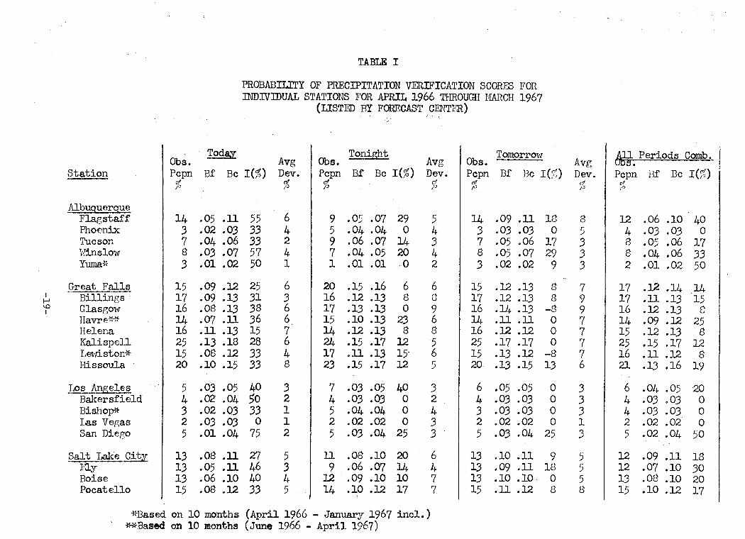
TABLE I

PROBABILITY OF PRECIPITATION VERIFICATION SCORES FOR INDIVIDUAL STATIONS FOR APRIL 1966 THROUGH HARCH 1967

(LISTED BY FORECAST CllJTER)

Avg Obs. Avg 0 TomorrO't'l

ibs. --Station I Pcpn Bf Be I(%) Dev.

I Tonight

Pcpn Bf Be I(%) Dev. Pcpn Bf Be I(:n of o! a! d o! ij /0 p /a I"

I Albuguergue

Flagstaff 14 .05 .11 55 6 9 .05 .07 29 5 14 .09 .11 18 Phoenix 3 .02 .03 33 4 5 .04 .04 0 4 3 .03 .03 0 Tucson 7 .04 .06 33 2 9 .06 .07 14 3 7 .05 .06 17 1·rinslow 8 .03 .07 57 4 7 .04 .05 20 4 8 .05 .07 29 Yuma* 3 .01 .02 50 1 1 .01 .01 .o 2 3 .02 .02 9

great Falls 15 .09 .12 25 6 20 .15 .16 6 6 15 .12 .13 8 Billings· 17 .09 .13 31 3 16 .12 .13 8 n 17 .12 .13 8 u

Glase;o11 16 .08 .13 38 6 17 .13 .lJ 0 9 16 .14 .13 -8 Havre-!:-~ 14 .07 .11 36 6 15 .10 .13 23 6 14 .11 .11 0 Helena 16 .11 .13 15 7 14 .12 .13 8 8 16 .12 .12 0 Kalispell 25 .13 .18 28 6 24 .15 .17 12 5 25 .17 .17 0 Lm·r.i.ston* 15 .08 .12 33 4 17 .11 .13 15 6 15 .13 .12 -8 Hissoula 20 .10 .15 33 8 23 .15 .17 12 5 20 .13 .15 13

Los Angeles 5 .03 .05 40 3 7 .03 .05 40 3 6 .05 .05 0 Bakersfield 4 • 02' .04 50 2 4 .03 .03 0 2 4 .03 .03 0 BishoP* 3 .02 .03 33 1 5 .04 .04 0 4 3 .03 .03 0 Las Vegas 2 . 03 .03 0 1 2 .02 .02 0 3 2 .02 .02 0 San Diego 5 .01 .04 75 2 5 .03 .04 25 3 5 .03 .04 25

palt Lake City 13 .08 .11 27 5 11 .08 .10 20 6 13 .10 .11 9 Ely 13 .05 .11 46 3 9 .06 .07 14 4 13 .09 .11 18 Boise 13 .06 .10 40 4 12 .09 .10 10 7 13 .10 .10 0 Pocatello 15 .08 .12 33 5 14 .10 .12 17 7 15 .11 .12 8

-ll-Based on 10 months (April 1966 - January 1967 incl. ) **Based on 10 months (June 1966 - April 1967)

Avg ~ Periods Comb.

Dev. Pcpn Bf De I(%) c1 of jJ iJ

8 12 .06 .10 40 5 4 .03 .03 0 3 8 .05 .06 17 3 8 .04 .06 33 3 2 .01 .02 50

7 17 .12 .14 14 9 17 .11 .13 15 9 16 .12 .13 8 7 14 .09 .12 25 7 15 .12 .13 ,..,.

0

7 25 .15 .17 12 7 16 .11 .12 8 6 21 .13 .16 19

3 6 .04 .05 20 3 4 .03 .03 0 '2 4 .03 .03 0 --' 1 2 .02 .02 0 '2 5 .02 .04 50 --'

5 12 .09 .11 18 r :::> 12 .07 .10 30 5 13 .08 .10 20 8 15 .10 .12 17

I N ·a

I

Station

San Francis~o Eureka

.. Fresno : R,ed. Bl1ltf ·Reno

Sacramento Santa Haria Stockton

·I·Jinnemucca

Seattle Astoria Eugene Hedford Olympia Pendleton Portland Salem Spokane Halla \·Jal.la * I·Jenatchee * Yal~

TABLE~ I (CONT:INUED)

PROBABILITY OF :PRECIPTIATION VERIFICATION SCORES' :FOR INDIVIDUAL STATIONS FOR APRTI. 1966 TiffiOUGH HARCH. 1967

. (LISTED. BY, FORECAST CENTER)

· Today

Obs. Avg Pcpn Bf Be I(%) Dev.

crf . • ••. cf ;o· "JO

ll .05 .09 44 21 .05 .13 62

7 /02 .06 67 10 .02 .·09 78

6 ~04 .05 20 10 .04 .08 50 10 ~02 .07 71

8 .04 ~07 43 10 .'04 ~08 50

33 .i4 :19 2i 48 .ll .20 55 25 .07 ~16 56 is .en ~14 50 34 .09 ~i9 53 16 .08 .13 39 31 .09 .18 50 32 .ll .19 42 20 .12 .15 20 ..

. 18 .05 .• 13 62 8 .04 .08 50 9 .03 .07 57

4 4 2 2 4 2 3 2 4

6 8 6 5 5 6 7 8 8• 5 7 4

Tonight

Obs. Avg Pcpn Bf Be I(%) Dev.

of . % ;o

10 .05 .08 38 21 .10 .14 29

6 .04 .o6 33 ll .07 .09 22 ··a .o6 ~07 14 10 •• 05 ~·oa 38

7 :o4 .o? 43 9 .()4 .07 43

11 .07 .09 22

32 46 23 18 35 15 27 29 16 19

. 9 I 9

~i6 ~19 16 .17 .2o 15 .10 :15 33 ~ll .14 21 .16 :19 16 .11 .12 8 .15 .18 17 .14 .17 18 .10 .12 . 8 ~10 .14 29 :o6 ·.os 25 .07 .08 13 \

4 6 4 7 4 4 4 3 5

8 12

5 7 7 5 9 9 8 5 7 7

Tomorrow

Obs. Avg Pcpn Bf Be I(;,~) Dev.

o1 ~ ;o rJ

ll .• 07 .09 22 21 .11 .14 21

7 .05 .:06 17 10 .08 .09 11 6 .05 .06 17

10 .06 .07 14 10 .06 .07 14

8 .06 .06 0 10 .07 .08 13

33 48 25 18 34 16 31 32 20~

. 18 I a I 9

.18 .19 5

.19 .20 5

.12 .15 20

.13 .14 7

.15 .20 25

.13 .12 -8

.17 .17 0

.19 .18 -6

.13 .15 13 ;],2 .l3' 8 .08 .09 11 .07 .07 0

5 8 5 7 6 5 6 5 5

8 ll 6 6 5 8 8

13 7 9 7 5

i~Based on 10 months (April 1966·::~::J~in~ :--196'7~incL) · •. · .. ··" ,; ...... ' .. · . • .. •. c_ ... ·.},J .. ··:.· •: ..

. l: '~~!.__,_.,.

. All Periods Comb. ~=~:.,..;:;::=;..;::.::.....=.=::..::.

Obs. Pcpn Bf . Be I(%)

d f'J

ll .06 .09 J3 21 .09 .. 14 36 . 7 :04 -~06 33 10 .06 .• 09 33 7 .05 :o6 17

10 • 05 .:os 38 .. 9 .04 ."07 43

8 .05 .07 29 10 .06 .08 25

33 .16 .19 16 47 .16 .20 20 24 .10 .15 33 18 .10 .14 29 34 .14 .19 26 16 .ll .12 8 30 .14 .18 22 31 .15 .18 17 19 .12 .14 14 18 .09 ~13 -<j1

8 .06 .08 25 9 .06 .07 14

Western Region Technical Memoranda: (Continued)

No. 24 Historical and Climatological Study of Grinnell Glacier, Montana. Richard A. Dightman. July 1967.