UNIVERSITY OF OSLODepartment of Informatics

Verification ofNetworkSimulatorsThe good, the bad andthe ugly

Master thesis

Mats Rosbach

21st November 2012

Verification of Network Simulators

Mats Rosbach

21st November 2012

ii

Contents

1 Introduction 11.1 Background and motivation . . . . . . . . . . . . . . . . . . . 11.2 Problem definition . . . . . . . . . . . . . . . . . . . . . . . . 21.3 Contributions . . . . . . . . . . . . . . . . . . . . . . . . . . . 31.4 Outline . . . . . . . . . . . . . . . . . . . . . . . . . . . . . . . 3

2 Background 52.1 Evaluation of systems . . . . . . . . . . . . . . . . . . . . . . 52.2 Network simulators . . . . . . . . . . . . . . . . . . . . . . . . 6

2.2.1 Simulation models . . . . . . . . . . . . . . . . . . . . 62.2.2 What characterizes a network simulator? . . . . . . . 62.2.3 Discrete Event Simulators . . . . . . . . . . . . . . . . 72.2.4 The use of network simulators . . . . . . . . . . . . . 8

2.3 Network emulators . . . . . . . . . . . . . . . . . . . . . . . . 92.4 Transmission Control Protocol . . . . . . . . . . . . . . . . . . 10

2.4.1 Selective acknowledgements . . . . . . . . . . . . . . 122.4.2 Nagle’s algorithm . . . . . . . . . . . . . . . . . . . . . 132.4.3 TCP Congestion control . . . . . . . . . . . . . . . . . 132.4.4 NewReno . . . . . . . . . . . . . . . . . . . . . . . . . 162.4.5 BIC and CUBIC . . . . . . . . . . . . . . . . . . . . . . 17

2.5 Queue management . . . . . . . . . . . . . . . . . . . . . . . 192.6 Traffic generation . . . . . . . . . . . . . . . . . . . . . . . . . 20

2.6.1 Tmix - A tool to generate trace-driven traffic . . . . . 212.7 The TCP evaluation suite . . . . . . . . . . . . . . . . . . . . . 23

2.7.1 Basic scenarios . . . . . . . . . . . . . . . . . . . . . . 242.7.2 The delay-throughput tradeoff scenario . . . . . . . . 282.7.3 Other scenarios . . . . . . . . . . . . . . . . . . . . . . 292.7.4 The state of the suite . . . . . . . . . . . . . . . . . . . 29

3 The TCP evaluation suite implementation 333.1 ns-2 . . . . . . . . . . . . . . . . . . . . . . . . . . . . . . . . . 33

3.1.1 Introduction . . . . . . . . . . . . . . . . . . . . . . . . 333.1.2 The evaluation suite implementation . . . . . . . . . 34

3.2 ns-3 . . . . . . . . . . . . . . . . . . . . . . . . . . . . . . . . . 363.2.1 Introduction . . . . . . . . . . . . . . . . . . . . . . . . 363.2.2 Tmix for ns-3 . . . . . . . . . . . . . . . . . . . . . . . 393.2.3 The evaluation suite implementation . . . . . . . . . 40

iii

3.3 OMNeT++ . . . . . . . . . . . . . . . . . . . . . . . . . . . . . 463.3.1 Introduction . . . . . . . . . . . . . . . . . . . . . . . . 473.3.2 Tmix for OMNeT++ . . . . . . . . . . . . . . . . . . . 513.3.3 The evaluation suite implementation . . . . . . . . . 61

4 Simulation results 674.1 Introduction . . . . . . . . . . . . . . . . . . . . . . . . . . . . 674.2 The expected results . . . . . . . . . . . . . . . . . . . . . . . 684.3 ns-2 results . . . . . . . . . . . . . . . . . . . . . . . . . . . . . 694.4 ns-3 results . . . . . . . . . . . . . . . . . . . . . . . . . . . . . 754.5 OMNeT++ results . . . . . . . . . . . . . . . . . . . . . . . . . 794.6 Comparison . . . . . . . . . . . . . . . . . . . . . . . . . . . . 864.7 Discussion . . . . . . . . . . . . . . . . . . . . . . . . . . . . . 87

4.7.1 Tmix . . . . . . . . . . . . . . . . . . . . . . . . . . . . 89

5 Conclusion 915.1 Future work . . . . . . . . . . . . . . . . . . . . . . . . . . . . 93

A ns-3 README 95A.1 Prerequisites and installation . . . . . . . . . . . . . . . . . . 95A.2 Usage . . . . . . . . . . . . . . . . . . . . . . . . . . . . . . . . 95

B OMNeT++ README 97B.1 Prerequisites . . . . . . . . . . . . . . . . . . . . . . . . . . . . 97B.2 How to run the evaluation suite in OMNeT++ . . . . . . . . 97

C Contents of CD-ROM 99

iv

List of Figures

2.1 Simple tcp example . . . . . . . . . . . . . . . . . . . . . . . . 112.2 TCP’s basic slow-start and congestion avoidance algorithm . 152.3 TCP Reno with fast retransmit and fast recovery . . . . . . . 162.4 BIC and its three phases . . . . . . . . . . . . . . . . . . . . . 182.5 CUBIC’s growth function . . . . . . . . . . . . . . . . . . . . 192.6 Typical HTTP session . . . . . . . . . . . . . . . . . . . . . . . 212.7 Simplified BitTorrent session . . . . . . . . . . . . . . . . . . 222.8 Simple dumbbell topology with standard delays . . . . . . . 252.9 Congestion collapse . . . . . . . . . . . . . . . . . . . . . . . . 31

3.1 TCP/IP stack in OMNeT++ . . . . . . . . . . . . . . . . . . . 483.2 Basic overview of tmix components . . . . . . . . . . . . . . 523.3 A DelayRouter and its submodules . . . . . . . . . . . . . . . 563.4 Callee map before optimization for tmix OMNeT++ . . . . . 583.5 Improved callee map for tmix OMNeT++ . . . . . . . . . . . 593.6 Final callee map for tmix OMNeT++ . . . . . . . . . . . . . . 593.7 Dumbbell topology shown in OMNeT++ . . . . . . . . . . . 63

4.1 ns-2 - delay-throughput tradeoff scenario - Throughput . . . 734.2 ns-2 - delay-throughput tradeoff scenario - Queueing delay . 734.3 ns-2 - delay-throughput tradeoff scenario - Drop rate . . . . 744.4 ns-3 - delay-throughput tradeoff scenario - Throughput . . . 774.5 ns-3 - delay-throughput tradeoff scenario - Queueing delay . 784.6 ns-3 - delay-throughput tradeoff scenario - Drop rate . . . . 784.7 OMNeT++ - delay-throughput tradeoff scenario - Throughput 854.8 OMNeT++ - delay-throughput tradeoff scenario - Queueing

delay . . . . . . . . . . . . . . . . . . . . . . . . . . . . . . . . 854.9 OMNeT++ - delay-throughput tradeoff scenario - Drop rate 86

v

vi

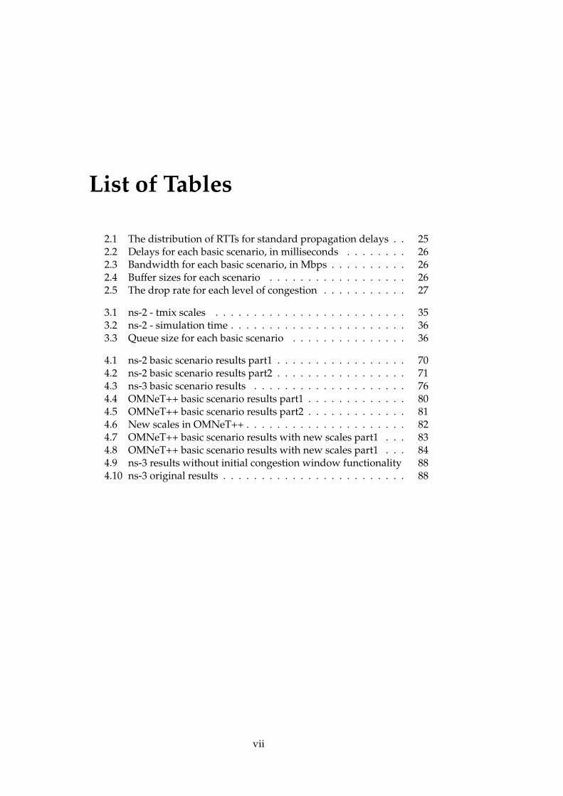
List of Tables

2.1 The distribution of RTTs for standard propagation delays . . 252.2 Delays for each basic scenario, in milliseconds . . . . . . . . 262.3 Bandwidth for each basic scenario, in Mbps . . . . . . . . . . 262.4 Buffer sizes for each scenario . . . . . . . . . . . . . . . . . . 262.5 The drop rate for each level of congestion . . . . . . . . . . . 27

3.1 ns-2 - tmix scales . . . . . . . . . . . . . . . . . . . . . . . . . 353.2 ns-2 - simulation time . . . . . . . . . . . . . . . . . . . . . . . 363.3 Queue size for each basic scenario . . . . . . . . . . . . . . . 36

4.1 ns-2 basic scenario results part1 . . . . . . . . . . . . . . . . . 704.2 ns-2 basic scenario results part2 . . . . . . . . . . . . . . . . . 714.3 ns-3 basic scenario results . . . . . . . . . . . . . . . . . . . . 764.4 OMNeT++ basic scenario results part1 . . . . . . . . . . . . . 804.5 OMNeT++ basic scenario results part2 . . . . . . . . . . . . . 814.6 New scales in OMNeT++ . . . . . . . . . . . . . . . . . . . . . 824.7 OMNeT++ basic scenario results with new scales part1 . . . 834.8 OMNeT++ basic scenario results with new scales part1 . . . 844.9 ns-3 results without initial congestion window functionality 884.10 ns-3 original results . . . . . . . . . . . . . . . . . . . . . . . . 88

vii

viii

Acknowledgements

I would like to thank my supervisors, Andreas Petlund and Michael Welzl,for helping me with my thesis, answering question and providing valuablefeedback. Thanks to the guys at the lab for keeping me company on ourjourneys to the coffee machine. And finally, thank you Kathinka, my dear,for kicking me out of bed in the morning... and for the moral support.

ix

x

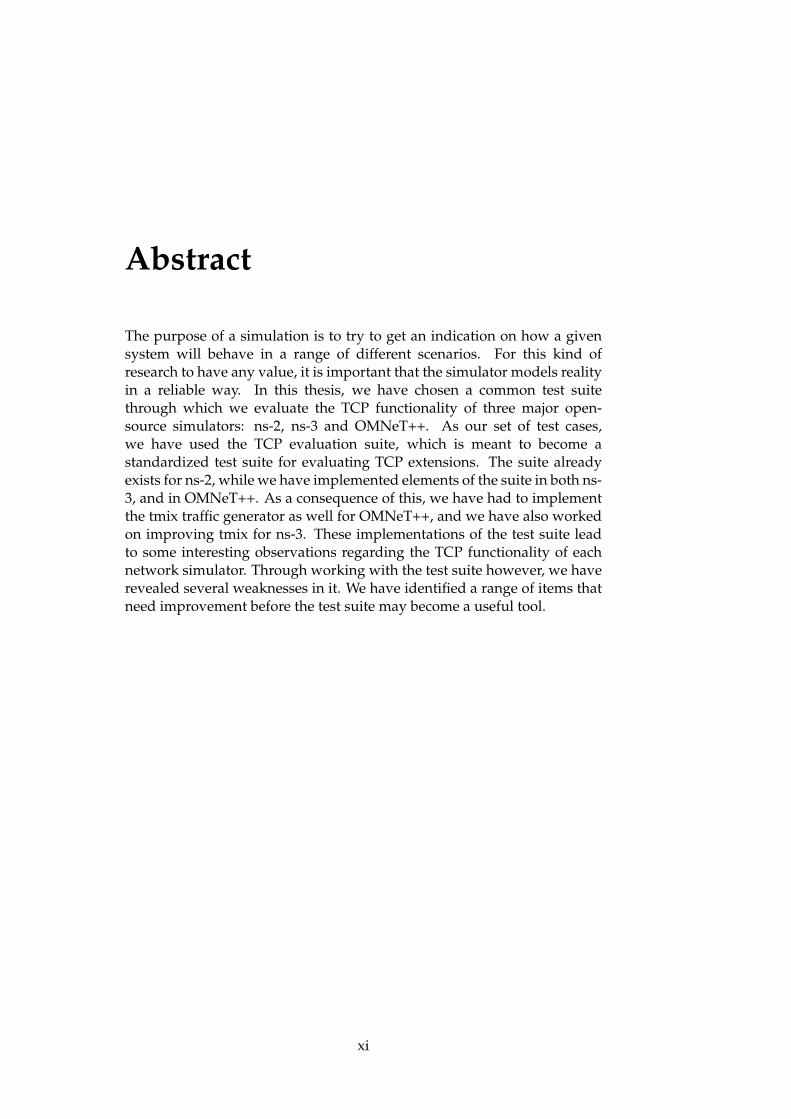
Abstract

The purpose of a simulation is to try to get an indication on how a givensystem will behave in a range of different scenarios. For this kind ofresearch to have any value, it is important that the simulator models realityin a reliable way. In this thesis, we have chosen a common test suitethrough which we evaluate the TCP functionality of three major open-source simulators: ns-2, ns-3 and OMNeT++. As our set of test cases,we have used the TCP evaluation suite, which is meant to become astandardized test suite for evaluating TCP extensions. The suite alreadyexists for ns-2, while we have implemented elements of the suite in both ns-3, and in OMNeT++. As a consequence of this, we have had to implementthe tmix traffic generator as well for OMNeT++, and we have also workedon improving tmix for ns-3. These implementations of the test suite leadto some interesting observations regarding the TCP functionality of eachnetwork simulator. Through working with the test suite however, we haverevealed several weaknesses in it. We have identified a range of items thatneed improvement before the test suite may become a useful tool.

xi

xii

Chapter 1

Introduction

1.1 Background and motivation

Network researchers must test Internet protocols under a variety ofdifferent network scenarios to determine whether they are robust andreliable. In some cases it is possible to build wide-area testbeds to performsuch testing, but in many cases testing the protocol through a real worldimplementation is impossible. This is due to the complexity and difficultiesin building, maintaining and configuring real world tests or testbeds. Analternative way of performing such testing is through the use of a networksimulator.

The purpose of a simulation is to try to get an indication on how theprotocol in question will behave in the real world. For this kind of researchto have any value, it is important that the network simulator acts as it issupposed to do, i.e., like a real network. A network simulator, opposedto a real network, runs only as software. This means that every part ofthe network must be modelled and implemented by a developer. This,for instance, includes models of the physical equipment, such as cables orwireless signals, models of networking protocols, such as TCP and IP, orapplication-layer protocols, such as HTTP and FTP. Every detail from thereal world cannot possibly be included in the simulation, and the problemis to decide which details are significant, and which are not. Choosingthe correct abstraction level suitable for the simulation is one of the keychallenges for the simulator developer. As an example of abstraction,consider the question on how time should be handled. Time as we knowit in the real world is continuous, which means that there is no smallestamount of time that we can measure. If we measure nanoseconds forinstance, there is always the possibility of measuring a smaller amountof time, namely picoseconds. In digital computers however, a smallestamount of time must be defined. When choosing an abstraction level,the scenario to be investigated must be considered. In network researchwe often measure delays in milliseconds or microseconds, so the simulatorwill obviously have to support measurements in microseconds. Hardware,such as central processing units (CPUs), works with much smaller amountsof time. The developer of a network simulator will at some point have

1

to make a decision and choose an appropriate abstraction level. This is atradeoff between simulator performance, realism and simplicity.

Simulating real networks, and especially complex networks like theInternet, is difficult. Floyd and Paxson [21] concludes their discussionon simulating the Internet by saying that "In many respects, simulatingthe Internet is fundamentally harder than simulation in other domains. In theInternet, due to scale, heterogeneity and dynamics, it can be difficult to evaluatethe results from a single simulation or set of simulations. Researchers need totake great care in interpreting simulations results and drawing conclusions fromthem". This quote brings us to another potential problem with networksimulators: actually using the simulator. A network simulator is a complexsystem that can be quite overwhelming to use. There are a lot of details thatthe researcher has to take into consideration while designing his simulationscenario. First of all there is the question of whether the scenario resemblesa real world scenario. How realistic is the model? Then there is the problemof actually verifying that the model has been implemented as intended inthe network simulator.

When publishing networking research papers, criticism is often basedon the community’s esteem of the simulator that was used. To the bestof our knowledge, a systematic comparison of different simulators withreference to real life Internet tests has not been performed. In this workwe aim to create test scenarios that can be used to compare and evaluatenetwork simulators and analyse the results.

1.2 Problem definition

Network simulators are complex systems, and we have to limit this thesisto parts of the topic. We have chosen to focus our work on TCP and itscongestion control algorithms. This means that we have chosen a set of testcases that specifically highlight the fundamental principles of TCP.

We have chosen a common set of test cases, which is implementedand evaluated in three open-source network simulators: ns-2, ns-3 andOMNeT++. We wanted to test commercial simulators as well, likeOPNET [11] and EstiNet [3], but were unable to acquire them for ourexperimentation.1

As our set of test cases, we have chosen the TCP evaluation suite, whichwas originally the outcome of a round-table meeting, summarized by Floydet al. [17], but has further been developed by David Hayes. The TCPevaluation suite describes a common set of test cases meant to be used byresearchers to quickly get a basic evaluation of proposed TCP extensions.This evaluation suite seemed to have a reasonable set of test cases, and as a

1OPNET has a university program in which researchers and students may apply for alicense of the simulator at discount prices. As stated on their web page however, one has to"Agree that the software shall not be used for any comparative studies with competing simulationpackages" before applying for this license. This made it difficult for us to apply for such alicense. We did not receive any reply from EstiNet when we contacted them about a licensefor our experiments.

2

side-effect, the implementation of the suite could be useful to the researchcommunity as well.

We have investigated three basic TCP variants: Tahoe, Reno, andNewReno. It would have been interesting to run newer variants as well(such as CUBIC), but due to limitations in the TCP functionality of ns-3and OMNeT++, we have been unable to do so. The three variants are runthrough the TCP evaluation suite in each simulator to try to see whethereach of them behaves in the way one would expect them to, but also tosee how the three network simulators compare to each other. This thesiswill investigate whether the differences between simulators are small, orwhether the tested simulators deviate enough that the results may bequestioned.

1.3 Contributions

There is no doubt that the network research community could benefit fromhaving a standardized set of test cases, to be used as an initial evaluationof new TCP extensions. As part of this thesis, we have developed elementsof the TCP evaluation suite in both OMNeT++ and ns-3 (the ns-2 versionof the suite is already available online). As a consequence of this, we havealso needed to implement the tmix traffic generator for OMNeT++, andhave worked on improving tmix for ns-3.

Through the TCP evaluation suite implementation, we have evaluatedthe TCP functionality of the three network simulators. We have come to theconclusion that ns-2 has by far the richest TCP functionality of the three.ns-3 and OMNeT++ only have very basic TCP algorithms built-in: Tahoe,Reno and NewReno, as well as TCP without congestion control. In additionto this, both simulators are in the process of integrating the NetworkSimulation Cradle, which makes it possible to run real-world protocolstacks in a simulated environment. This would be a great enhancementto the TCP functionality of both of them.

The suite is still a work in progress, and will need to undergo majorchanges before it can be standardized and used as a tool to evaluate TCPextensions. We have evaluated the current state of the suite against threemajor open-source simulators. Through this evaluation, we have workedwith the tmix traffic generator, which we argue has several flaws in itsdesign that should be looked into. We have, as far as we know, been thefirst to try the TCP evaluation suite in practice, and our experience is thatit is not at all ready yet.

1.4 Outline

The thesis is organized as follows. In chapter 2 we present backgroundinformation relevant to our work. This includes general information aboutnetwork simulators and emulators, TCP and congestion control, the TCPevaluation suite and tmix. In chapter 3 we present the evaluation suite

3

implementation in ns-2, ns-3, and OMNeT++ respectively. In chapter 4 wepresent our results, and we conclude the thesis in chapter 5.

4

Chapter 2

Background

This chapter contains background information necessary to understandthis thesis. It will briefly summarize how systems can be evaluated, withfocus on network simulators, it will draft the functionality of TCP and someof its variants. A common TCP evaluation suite has been proposed, and isdescribed in this chapter, as well as a discussion on traffic generation ingeneral.

2.1 Evaluation of systems

In general there are three different techniques to evaluate the performanceof a system or a network; analytical modelling, simulation, or measure-ments [35]. All of these have their strengths and weaknesses. Each of theevaluation techniques is weak on their own, but a combination of them allshould give thorough evaluation of the system.

Analytical modelling is a highly theoretical technique where a systemis analysed by investigating mathematical models or formal proofs. Thestrength of such a technique is that it can be performed very early inthe development process, before any time and money has been spent onactually implementing the system. It is a technique that evaluates theidea and the design of a system, and may give a basic indication on howwell the system will perform, without going into specifics. The downsideof analytical modelling is that it is largely based on simplifications andassumptions, as the actual system is not involved in the evaluation. Thisgives analytical modelling a low accuracy.

Simulations are closer to reality than analytical modelling, but stillabstract away details. Simulations can be performed throughout the entiredevelopment process. They can early on give a good indication on howwell the system will perform, but also be used in later stages of the processto find flaws in the design. Another strength of simulation, is that it is easyto perform large-scale tests that otherwise would be difficult to implementin a test-bed, or in the actual system itself.

Another technique of performing system evaluation is to take measure-ments of the actual system. Investigating the real system requires at leastparts of the system be implemented. Testing on the real system will of

5

course give very accurate results, but at the cost of having to implement itbefore being able to evaluate it. Finding flaws in the design at this pointis costly. The system does not have to be implemented fully, setting up asmall-scale test-bed, or developing a prototype of the system is also pos-sible, but this requires a lot of work as well.



2.2 Network simulators

2.2.1 Simulation models

A model is an object that strives to imitate something from the real world.This model cannot entirely recreate the real world object, and will haveto abstract away some of its details. There are several types of simulationmodels out there. We will explain some of the major differences using afew basic attributes. Simulation models vary on whether they are dynamicor static. They may be deterministic or stochastic, and they may be discreteor continuous. These terms are important when describing models.

A dynamic model is a model that depends on time, in which statevariables change over time. This could for instance be a model of acomputer network that runs over several hours, where the state of eachcomponent varies depending on the traffic generated. A static model onthe other hand, concerns itself with only snapshots of the system.

A deterministic model is a model in which the outcome can bedetermined by a set of input values. This means that if a simulation usinga deterministic model is run several times using the same input values, theresult will always be the same. In stochastic models on the other hand,randomness is present.

In discrete models, the state variables only change at a countableamount of times. Discrete models define the smallest unit of timesupported, and events may only happen at these discrete times. This isopposed to continuous models, where state variables can change whenever,and the number of times in which events may happen is infinite.

2.2.2 What characterizes a network simulator?

A network simulator, as opposed to a real network, runs only as software.A network simulator must therefore consist of software that representseverything in a real network. This includes software for the physicalequipment, like cables and wireless signals. It includes software thatrepresents the connection points or the endpoints in the network, forinstance a web server or a router. Depending on the network to besimulated, a protocol stack must be in place, for instance when simulatingthe Internet, network protocols such as IP, TCP and UDP must be in place.And lastly, some application (as well as a user using the application) isnecessary to generate traffic on the network.

As already mentioned, simulations are based on different types ofmodels. What attributes do we find in network simulators? It is possible

6

for network simulators to be either dynamic or static. A very common typeof network simulator, a Discrete Event Simulator (DES), is a good exampleof dynamic simulator. These are simulators where events are scheduleddynamically as time passes. On the other hand, we have Monte Carlosimulations, which are static. This is a type of simulation that relies onrepeated sampling to compute the result. Monte Carlo simulations are usedto iteratively evaluate a model by using sets of random numbers as inputs.These types of simulations are often used when the model is complexand involves a lot of uncertain parameters. The model may be run manythousands of times with different random inputs, where the final resultof the entire simulation typically is a statistical analysis of all the resultscombined. Monte Carlo simulation is especially useful for simulatingphenomena with significant uncertainty in inputs, and for systems of highcomplexity. Computer networks however are usually well understood (atleast compared to some mathematical and physical sciences where MonteCarlo simulations are usually used), and should not require an iterativemethod such as Monte Carlo to get representative results.

Computer simulations are in general discrete. The real world iscontinuous, as there are no rules that determine a smallest measure of timein which every event must occur. Mathematical models may be continuous.For instance, consider the function f(x). The value of f(x) depends entirelyon x, and as there are no limitations on the values of x, the range of valuesfor f(x) is infinite. This is something that is difficult to achieve in computersimulations, and is only possible in analogue computers. When usingdigital computers, it is possible to achieve something close to a continuoussimulation by making each time step really small, but it theory it willalways be a discrete simulation. There is always the question of how muchaccuracy is really needed, and continuous time is something that networksimulators abstract away from. For instance, in OMNeT++ it is possible todetermine time down to a precision of 10−18 seconds. The question is: dowe really need more?

As most network simulators are DESs, according to Wehrle et al. [35],we will only go into detail about DESs.

2.2.3 Discrete Event Simulators

DESs are described in [35], which includes most network simulators outthere. A DES consists of a number of events that occur at discretetimes during the run of the simulation. Discrete in this case means thatthe simulator is defined for a finite or countable set of values, i.e., notcontinuous, which means that there is defined a smallest measure of timein which an event can occur. Two consecutive events cannot occur closertogether in time than the smallest measure of time dictates, althoughseveral events may occur at the same time. Below is a list of a few importantterms in DESs:

• An entity is an object of interest in the system to be modelled. Forinstance, in a network simulation, an entity could be a node or a link

7

between two nodes.

• A model is an object in the simulator that imitates an entity from thereal world. As an example we can use the model of a laptop. Mostnetwork simulators abstract away from most details of this laptop.In ns-3 for instance, all laptops, desktop computers, servers, routers,switches etc. in the network are simply called nodes. There is noinformation about the hardware of a node in ns-3 as a result of theabstraction level the designers chose when developing ns-3.

• Attributes describe certain aspects of an entity. A network channelmay have attributes such as bandwidth and latency, while a trafficgenerator may have attributes such as inter-arrival time and averagebit rate.

• A system consists of a set of entities and the relationships betweenthem. This set of entities might include nodes, a wireless channelconnecting the nodes, and models of a user that generates trafficthrough an HTTP application.

• A discrete system is a system where the states in the system onlychange at discrete points in time. The change of a state is triggeredby some event in the system. One such change might be dequeuing apacket for transmission over a communication channel. This changesthe state of the system as the packet is no longer located in thetransmission queue, but is now located on the channel betweennodes. Another event might be receiving a packet.

A simulation is a large model that is consisting of several sub-models thateach represents real-world entities, a collection of abstractions in otherwords. In addition to the simulation model, a simulation also includes away of generating input. The input is inserted into the simulator, which inturn makes the model act upon the input, thus generating output.

2.2.4 The use of network simulators

A network simulator imitates a specific environment as described inthe previous section. This environment contains abstractions from thereal world, abstractions for host machines, routers, wireless connections,fibre cables, user patterns and so on. Network simulators are typicallyused by researchers, engineers and developers to design various kinds ofnetworks, simulate and then analyse various parameters on the networkperformance.

In network education, there is need for practical hands-on skillsalongside the theory that students learn through a course. However,a dedicated network laboratory is expensive and is both difficult andexpensive to maintain. A better alternative is to use a network simulatorto give the students some kind of practical experience working withnetworks. Some network simulators, like ns-2, are designed for researchand may be too complex and difficult to use for educational purposes [32].

8

Other network simulators are designed in a way that makes them moresuitable for education. One example of such a simulator is Packet Tracer,which is an integral part of the Cisco Network Academy Program [25].Network simulators used in commercial development is outside the scopeof this thesis; however the benefits of using network simulators in researchshould also apply to development of commercial software.

2.3 Network emulators

An emulator is a piece of hardware or software that aims to duplicate (oremulate) the functions of a specific system. The emulator can be usedas a replacement for systems. The focus of an emulator is to reproducethe external behaviour of the original system as closely as possible. Thismeans that the emulator has to accept the same type of input that theoriginal system does, and also that it has to produce the same output. Inother words; the emulator has to perform the same function as the originalsystem. Note that the emulator can implement this functionality howeverit wishes to, as long as it looks as if it functions in the same way that theoriginal system does. Below are a couple of examples on how emulatorsmight be used.

Emulation is a common strategy to help tackle obsolescence. The newversions of Windows are a good example of how this works. When anew version of Windows is shipped, there are functions from previousWindows versions that are left obsolete. The obvious problem is howolder applications that rely on obsolete functions are supposed to continueworking as intended. The most intuitive way of handling this is to actuallyupdate the application, but this is not always possible as many olderapplications are not maintained any more. Another way of handling thisis to run the application on an emulator that emulates an older version ofWindows. In Windows there is the possibility of running an application incompatibility mode [37], which emulates the older Windows version. To theapplications, it seems like it is running on the older version of Window.

Another example is the Oracle VM VirtualBox [28], which emulates anentire computer. This can be used to run several operating systems onone machine, without having to actually install them on the real machine.It is useful for testing possibly malicious software, without running therisk of destroying anything useful on the computer. The operating systeminstalled on the virtual machine will think that it is in fact installed on a realmachine, because the emulator duplicates the functionality of a machine.

While the two previous examples were emulators, they were notnetwork emulators. Netem is an example of a network emulator. Netememulates certain properties of a wide area network. This includes havingthe possibility of modifying properties like delay, loss, duplication andre-ordering of packets. Netem appears to be an actual network to othersystems. Netem implements send and receive functions that other systemsmay use in the same way that it might in a real network. Being able to"control" the network in this way is useful when testing and verifying new

9

applications and protocols.

2.4 Transmission Control Protocol

In the TCP/IP reference model [34], the transport layer is the secondhighest layer and communicates directly with the application on both thesending and receiving side. In general the basic function of the transportlayer is to accept data from above, split it into smaller units if need be,and pass these units to the network layer. At the receiving end, thetransport layer will accept data from the network layer and deliver themto the receiving application. In the classic OSI model, the transport layeronly concerns itself with end-to-end communication, which means it is notinvolved in intermediate jumps on the route between sender and receiver.This is a simplification of the real world, as there are several protocols thatbreak the layering of the OSI model. For instance, the Address ResolutionProtocol (ARP) is a protocol that converts network layer addresses into linklayer addresses, thus operating in both the link layer, and the networklayer. Although the OSI model is highly simplified, it still gives a basicindication on what each type of protocol is supposed to do. The transportlayer offers the application a set of services. The type of service offeredhowever, depends on the transport layer protocol used. The three mostcommonly used transport layer protocols used in the Internet are: theTransmission Control Protocol (TCP) [31], the User Datagram Protocol(UDP) [30], and the Stream Control Transmission Protocol (SCTP) [33]. Thissection will describe the basics of TCP.

When the transport layer protocol hands over a segment to the networklayer, there is no guarantee that the segment is ever delivered to thereceiving end of the communication. TCP was specifically designed toprovide a reliable end-to-end byte stream over an unreliable network (suchas the Internet). The protocol offers simple send and receive functionsto the application. These send/receive functions guarantee that all dataare delivered in order and error-free. TCP is used in common applicationlayer protocols such as HTTP (web), SSH (secure data communication) andSMTP (e-mail). The protocol has several features to provide its services inthe best way possible:

• Reliable end-to-end communication - TCP ensures that every segment isdelivered to the receiving endpoint. Before handing a segment to thenetwork layer, a sequence number is assigned to the segment. WhenTCP receives a segment, it can use the sequence number to determinewhether a segment has been lost, or whether a segment has beenreceived out of order. The protocol replies with acknowledgements(ACKs) to tell the sender that a segment has been successfullyreceived, and that the sender now can forget about this segment. Byusing sequence numbers in this way, the receiving end can detectsegments that disappear on its route to the receiver. It will alsodetect whether any segments arrive out of order, and can reorder thesegments before delivering them to the application.

10

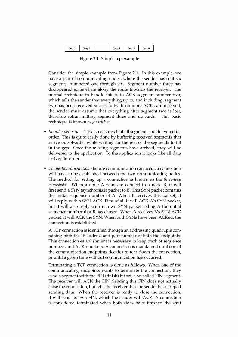
Figure 2.1: Simple tcp example

Consider the simple example from Figure 2.1. In this example, wehave a pair of communicating nodes, where the sender has sent sixsegments, numbered one through six. Segment number three hasdisappeared somewhere along the route towards the receiver. Thenormal technique to handle this is to ACK segment number two,which tells the sender that everything up to, and including, segmenttwo has been received successfully. If no more ACKs are received,the sender must assume that everything after segment two is lost,therefore retransmitting segment three and upwards. This basictechnique is known as go-back-n.

• In-order delivery - TCP also ensures that all segments are delivered in-order. This is quite easily done by buffering received segments thatarrive out-of-order while waiting for the rest of the segments to fillin the gap. Once the missing segments have arrived, they will bedelivered to the application. To the application it looks like all dataarrived in-order.

• Connection-orientation - before communication can occur, a connectionwill have to be established between the two communicating nodes.The method for setting up a connection is known as the three-wayhandshake. When a node A wants to connect to a node B, it willfirst send a SYN (synchronize) packet to B. This SYN packet containsthe initial sequence number of A. When B receives this packet, itwill reply with a SYN-ACK. First of all it will ACK A’s SYN packet,but it will also reply with its own SYN packet telling A the initialsequence number that B has chosen. When A receives B’s SYN-ACKpacket, it will ACK the SYN. When both SYNs have been ACKed, theconnection is established.

A TCP connection is identified through an addressing quadruple con-taining both the IP address and port number of both the endpoints.This connection establishment is necessary to keep track of sequencenumbers and ACK numbers. A connection is maintained until one ofthe communication endpoints decides to tear down the connection,or until a given time without communication has occurred.

Terminating a TCP connection is done as follows. When one of thecommunicating endpoints wants to terminate the connection, theysend a segment with the FIN (finish) bit set, a so-called FIN segment.The receiver will ACK the FIN. Sending this FIN does not actuallyclose the connection, but tells the receiver that the sender has stoppedsending data. When the receiver is ready to close the connection,it will send its own FIN, which the sender will ACK. A connectionis considered terminated when both sides have finished the shut

11

down procedure. A termination is not a three-way handshake likeconnection establishment, but rather a pair of two-way handshakes.Problems occur when packets are lost. For instance, consider thescenario where there are two nodes A and B. Node A has sent itsFIN and received an ACK on its FIN. Eventually B wants to close itsconnection as well. B sends its FIN, but never receives an ACK fromA. B does not know whether A received the FIN or not, and may retrysending the FIN. If A receives the FIN and replies with an ACK, howdoes A know whether B received the ACK or not? This problem hasbeen proved to be unsolvable. A work-around in TCP is that bothendpoints starts a timer when sending the FIN, and will close theconnection when the timer timeouts if they have not heard from theother end.

• Flow control - TCP uses a flow control protocol to ensure that thesender does not overflow the receiver with more data than it canhandle. This is necessary in scenarios where machines with diversenetwork speeds communicate, for instance when a PC sends datato a smartphone. In each TCP segment, the receiver specifies howmuch data it is willing to accept. The sender can only send up to thespecified amount of data before it must wait for ACKs.

• Congestion control - a mechanism to avoid the network becomingcongested. Congestion occurs when there is so much traffic on thenetwork that it exceeds the capacity of the links in the network.This forces the routers to drop frames, which in turn will beretransmitted by TCP when the drop is eventually noticed. Theretransmitted segments lead to more traffic, thus congesting thenetwork even more, which again leads to more retransmissions. Aftera while, performance collapses completely and almost no segmentsare delivered. It is in everyone’s interest that traffic is kept at sucha level that congestion does not occur. TCP’s congestion controlmechanism lowers the sending rate whenever congestion is detected,as indicated by the missing ACKs.

2.4.1 Selective acknowledgements

A simple technique to handle retransmissions has already been mentioned,namely go-back-n. The obvious drawback of go-back-n is that everysegment after a lost segment is retransmitted, regardless of whether theywere successfully received or not. An improvement over this is the use ofselective acknowledgements (SACK). Again, consider the simple examplein Figure 2.1. In this example, segment three has been lost. Another way tohandle the retransmission in this case, is to send a SACK back to the sender,with information on which segment has been dropped. Upon the receptionof this SACK, the sender now knows that only segment three has been lost,and can therefore retransmit only the lost segment.

SACK is more complex than go-back-n, and leads to much more over-head when drop rate is high, but to retransmit only the dropped segments,

12

rather than retransmitting the dropped segment and the succeeding seg-ments, can definitely be useful. Note that SACK is not a TCP variant onits own, but an alternative way of handling retransmissions that every TCPvariant may use.

2.4.2 Nagle’s algorithm

Nagle’s algorithm [26] is an algorithm that improves the efficiency of TCPby reducing the number of packets that needs to be sent. The algorithmis named after John Nagle. He describes what he calls the "small packetproblem". This is a scenario where TCP transmits a lot of small packets, forinstance single characters originating from a keyboard. The problem withthis is that for every single character that is to be sent, a full TCP/IP headeris added on top. This means that for each byte the application wants tosend, a 41 byte packet will be sent. This is obviously a problem in terms ofefficiency. The algorithm is simple: If there is unconfirmed data in the pipe,buffer data while waiting for an acknowledgement. If the buffer reaches thesize of a MSS, then send the segment right away. If there is no unconfirmeddata in the pipe, send the data right away. This solves the small packetproblem.

2.4.3 TCP Congestion control

Congestion control is one of the important features of TCP, as alreadymentioned briefly. This section will go through TCP’s congestion control inmore detail. There are several variants of TCP. Many of the earlier variantsare no longer being used because newer and better algorithms have beendeveloped, but there are still a number of variants out there. There is noanswer to which algorithm is the best one, as each variant has strengthsand weaknesses. Which variant to use depends on what attributes oneis interested in. For instance, some variants focus entirely on gettingthe highest possible throughput, some variants focus on fairness betweenflows, and some variants focus on getting as low a delay as possible. Wewill describe some of the earlier variants first, and describe TCP congestioncontrol as it has been improved over the years.

Tahoe

TCP Tahoe is one of the earliest TCP variants, and is quite basic comparedto the variants that we have today. Tahoe uses three algorithms to performcongestion control: slow start, congestion avoidance and fast retransmit.

Both the slow start, and the congestion avoidance algorithms, must beused by a TCP sender to control the amount of unacknowledged data thesender can have in transit. The sender keeps track of this by implementinga congestion window that specifies how much outstanding data he canhave at a given time, either in number of segments, or in number of bytes.If no congestion is detected in the network, the congestion window may

13

be increased. However, if congestion is detected, the congestion windowmust be decreased.

At the beginning of a transmission, the sender does not know theproperties of the network. It will slowly start probing the network todetermine the available capacity. Initially, the congestion window will betwo to four times the sender’s maximum segment size (MSS), which meansthat during the first transmission the sender can send two to four full-sizedsegments. When an ACK arrives, the sender may increase his congestionwindow by the size of one maximum segment. This means in theory thatthe congestion window doubles in size for every round-trip time (RTT)of the network. This exponential increase in window size continues untilthe slow start threshold, ssthresh, is reached. Initially, ssthresh should beset arbitrarily high so that the sender can quickly reach the limit of thenetwork, rather than some arbitrary host limit by setting ssthresh too low.ssthresh is later adjusted when congestion occurs. Whenever the congestionwindow is smaller than ssthresh, the slow start algorithm is used, andwhenever the congestion window is larger than ssthresh, the congestionavoidance algorithm is used.

During congestion avoidance, the congestion window is increasedby roughly one full-sized segment per RTT. This linear increase in thecongestion window continues until congestion has been detected. Whencongestion is detected, the sender must decrease ssthresh to half of thecurrent congestion window before entering a new slow start phase, wherethe congestion window is set to the initial congestion window size.

The basic slow start and congestion avoidance algorithm is shown inFigure 2.2. In this figure we can see the congestion window starting at 1024bytes at the first transmission (which means we have a maximum segmentsize of 512 bytes). For every transmission this congestion window doubles(increases exponentially) until it reaches the initial ssthresh, which is at32KB. After ssthresh has been reached, the congestion window increases by1024 bytes per transmission. After roughly 13 transmissions in this figure,a time-out occurs, which means that a segment probably is lost. This leadsto ssthresh being lowered to half of the current congestion window, beforestarting a new slow start phase.

When a receiver receives an out-of-order segment, the receiver shouldimmediately send a duplicate ACK message to the sender. From thereceiver’s point of view, an out-of-order segment can be caused by severalnetwork problems. The segment may arrive out-of-order because an earliersegment has been lost. It may arrive out-of-order because the order hasbeen mixed up in the network, and finally a segment may arrive out-of-order because either a segment or an ACK has been replicated by thenetwork. When a segment arrives out-of-order because an earlier segmenthas been lost, the chances are that several out-of-order segments will arriveat the same time. If for instance the sender has sent 10 segments at once,and segment number 4 has been lost, the receiver will receive the 3 firstsegments, then the last 6 segments roughly at the same time. This causesthe receiver to send several duplicate ACK messages at the same time, onefor each of 6 last segments. Therefore, upon the reception of 3 duplicate

14

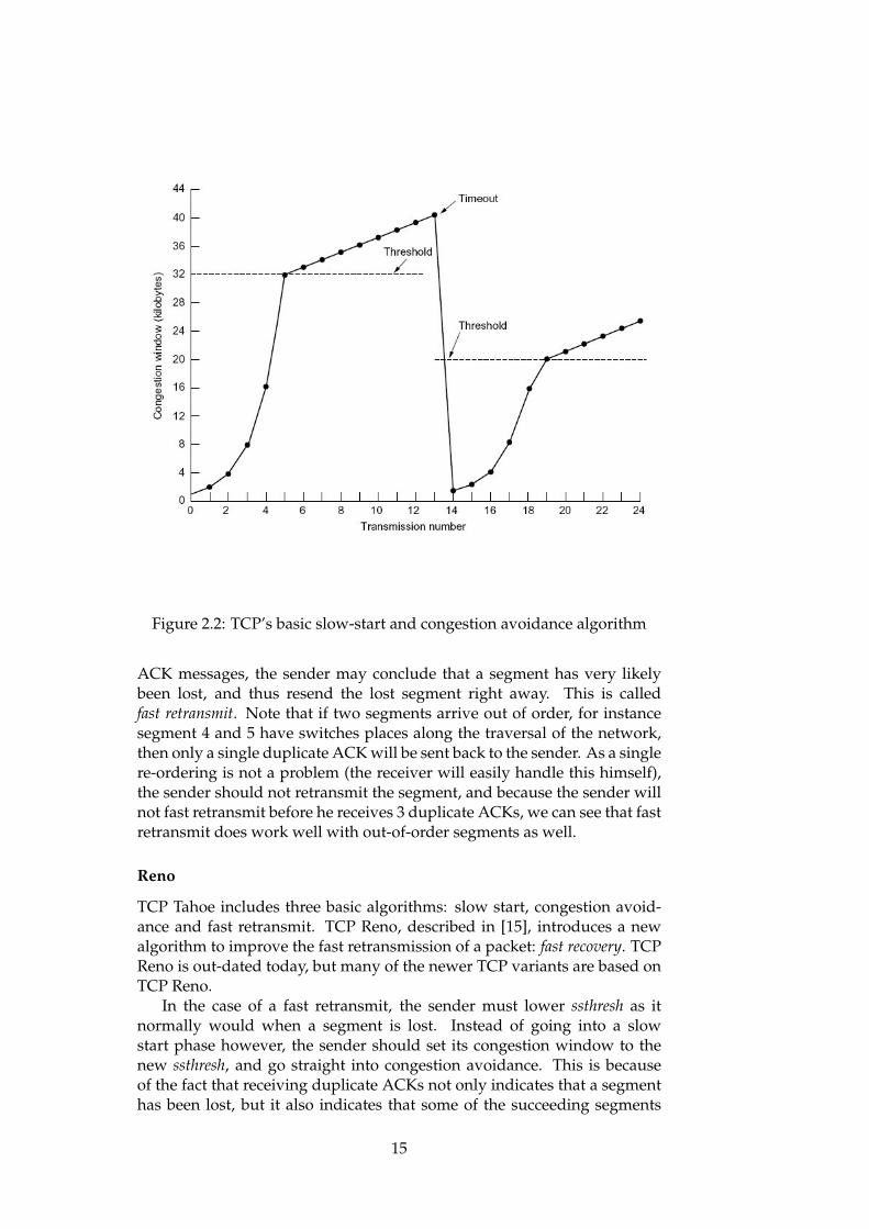
Figure 2.2: TCP’s basic slow-start and congestion avoidance algorithm

ACK messages, the sender may conclude that a segment has very likelybeen lost, and thus resend the lost segment right away. This is calledfast retransmit. Note that if two segments arrive out of order, for instancesegment 4 and 5 have switches places along the traversal of the network,then only a single duplicate ACK will be sent back to the sender. As a singlere-ordering is not a problem (the receiver will easily handle this himself),the sender should not retransmit the segment, and because the sender willnot fast retransmit before he receives 3 duplicate ACKs, we can see that fastretransmit does work well with out-of-order segments as well.

Reno

TCP Tahoe includes three basic algorithms: slow start, congestion avoid-ance and fast retransmit. TCP Reno, described in [15], introduces a newalgorithm to improve the fast retransmission of a packet: fast recovery. TCPReno is out-dated today, but many of the newer TCP variants are based onTCP Reno.

In the case of a fast retransmit, the sender must lower ssthresh as itnormally would when a segment is lost. Instead of going into a slowstart phase however, the sender should set its congestion window to thenew ssthresh, and go straight into congestion avoidance. This is becauseof the fact that receiving duplicate ACKs not only indicates that a segmenthas been lost, but it also indicates that some of the succeeding segments

15

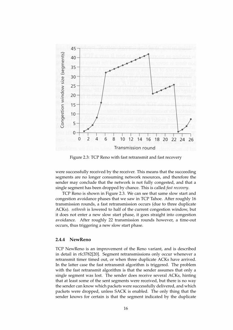
Figure 2.3: TCP Reno with fast retransmit and fast recovery

were successfully received by the receiver. This means that the succeedingsegments are no longer consuming network resources, and therefore thesender may conclude that the network is not fully congested, and that asingle segment has been dropped by chance. This is called fast recovery.

TCP Reno is shown in Figure 2.3. We can see that same slow start andcongestion avoidance phases that we saw in TCP Tahoe. After roughly 16transmission rounds, a fast retransmission occurs (due to three duplicateACKs). ssthresh is lowered to half of the current congestion window, butit does not enter a new slow start phase, it goes straight into congestionavoidance. After roughly 22 transmission rounds however, a time-outoccurs, thus triggering a new slow start phase.

2.4.4 NewReno

TCP NewReno is an improvement of the Reno variant, and is describedin detail in rfc3782[20]. Segment retransmissions only occur whenever aretransmit timer timed out, or when three duplicate ACKs have arrived.In the latter case the fast retransmit algorithm is triggered. The problemwith the fast retransmit algorithm is that the sender assumes that only asingle segment was lost. The sender does receive several ACKs, hintingthat at least some of the sent segments were received, but there is no waythe sender can know which packets were successfully delivered, and whichpackets were dropped, unless SACK is enabled. The only thing that thesender knows for certain is that the segment indicated by the duplicate

16

ACKs is lost. When several segments from the same window are lost, Renois not very effective, because it will take a full RTT before the retransmittedsegment is ACKed, and therefore it will also take a full RTT for each lostsegment to discover new lost segments. Another problem is that ssthreshis halved each time Reno fast retransmits a segment, which means ssthreshis halved for each segment lost, as it treats each loss individually. Notethat NewReno only applies to connections that are unable to use the SACKoption. When SACK is enabled, the sender has enough information aboutthe situation to handle it intelligently.

TCP NewReno differs from Reno on how it implements the fastretransmit and fast recovery algorithms. Upon entering fast recovery (afterreceiving 3 duplicate ACKs), ssthresh will be lowered to half of the currentcongestion window (cwnd), and then cwnd is set to ssthresh + 3 * SMSS.Reno will leave this fast recovery phase as soon as a non duplicate ACKis received, NewReno however does not. NewReno stays in the same fastrecovery phase until every segment in the window has been ACKed, thuslowering ssthresh only once.

NewReno works with what is called a partial acknowledgement, whichis an ACK that does not ACK the entire window. As long as the senderreceives partial ACKs, it will not leave the fast retransmit phase, butNewReno also includes another improvement over Reno. For everyduplicate ACK the sender receives, it will send a new unsent segment fromthe end of the congestion window. This is because the sender assumesthat every duplicate ACK stems from a successfully delivered segment,and therefore these segments are no longer in transmit, thus opening upfor new segments to be sent.

We can see that NewReno, just like Reno, still has to wait a full RTT todiscover each lost segment. However, not halving ssthresh for each segmentlost, and adding new segments to the transmit window for every duplicateACK received, is still a great improvement over Reno.

2.4.5 BIC and CUBIC

TCP BIC and TCP CUBIC [2] are two variants of TCP that focus onutilizing high-bandwidth networks with high latency. As demands for fastdownloads of large-sized data are increasing, so is the demand for a TCPvariant that can actually handle these transfers efficiently. The problemis that over high-latency networks, TCP does not react quickly enough,thus leaving bandwidth unused. TCP BIC is a congestion control protocoldesigned to address this problem.

BIC has a very unique window growth function which is quite differentto the normal TCP slow start and congestion avoidance algorithms. Whatis interesting is what happens when a segment is lost. When BIC noticesa loss, it reduces its window by a multiplicative factor. The window sizejust before the reduction is set to maximum (Wmax), while the windowsize after the reduction is set to minimum (Wmin). The idea is that becausea segment was lost at Wmax, equilibrium for this connection should besomewhere between Wmin and Wmax. BIC performs a binary search

17

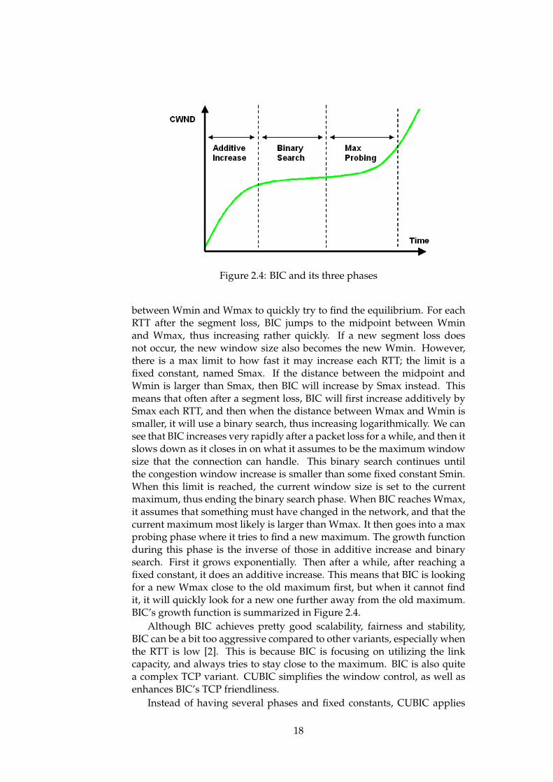
Figure 2.4: BIC and its three phases

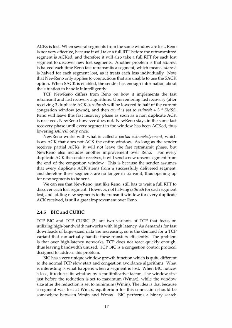
between Wmin and Wmax to quickly try to find the equilibrium. For eachRTT after the segment loss, BIC jumps to the midpoint between Wminand Wmax, thus increasing rather quickly. If a new segment loss doesnot occur, the new window size also becomes the new Wmin. However,there is a max limit to how fast it may increase each RTT; the limit is afixed constant, named Smax. If the distance between the midpoint andWmin is larger than Smax, then BIC will increase by Smax instead. Thismeans that often after a segment loss, BIC will first increase additively bySmax each RTT, and then when the distance between Wmax and Wmin issmaller, it will use a binary search, thus increasing logarithmically. We cansee that BIC increases very rapidly after a packet loss for a while, and then itslows down as it closes in on what it assumes to be the maximum windowsize that the connection can handle. This binary search continues untilthe congestion window increase is smaller than some fixed constant Smin.When this limit is reached, the current window size is set to the currentmaximum, thus ending the binary search phase. When BIC reaches Wmax,it assumes that something must have changed in the network, and that thecurrent maximum most likely is larger than Wmax. It then goes into a maxprobing phase where it tries to find a new maximum. The growth functionduring this phase is the inverse of those in additive increase and binarysearch. First it grows exponentially. Then after a while, after reaching afixed constant, it does an additive increase. This means that BIC is lookingfor a new Wmax close to the old maximum first, but when it cannot findit, it will quickly look for a new one further away from the old maximum.BIC’s growth function is summarized in Figure 2.4.

Although BIC achieves pretty good scalability, fairness and stability,BIC can be a bit too aggressive compared to other variants, especially whenthe RTT is low [2]. This is because BIC is focusing on utilizing the linkcapacity, and always tries to stay close to the maximum. BIC is also quitea complex TCP variant. CUBIC simplifies the window control, as well asenhances BIC’s TCP friendliness.

Instead of having several phases and fixed constants, CUBIC applies

18

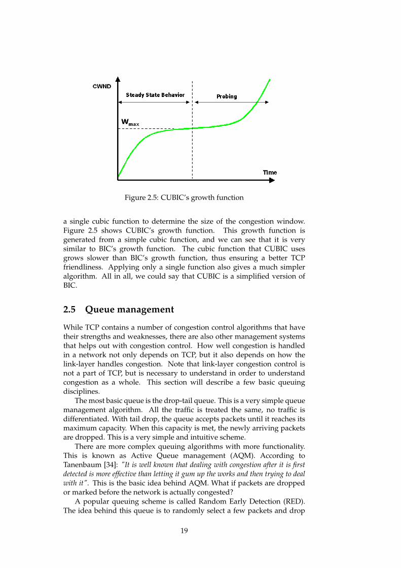
Figure 2.5: CUBIC’s growth function

a single cubic function to determine the size of the congestion window.Figure 2.5 shows CUBIC’s growth function. This growth function isgenerated from a simple cubic function, and we can see that it is verysimilar to BIC’s growth function. The cubic function that CUBIC usesgrows slower than BIC’s growth function, thus ensuring a better TCPfriendliness. Applying only a single function also gives a much simpleralgorithm. All in all, we could say that CUBIC is a simplified version ofBIC.

2.5 Queue management

While TCP contains a number of congestion control algorithms that havetheir strengths and weaknesses, there are also other management systemsthat helps out with congestion control. How well congestion is handledin a network not only depends on TCP, but it also depends on how thelink-layer handles congestion. Note that link-layer congestion control isnot a part of TCP, but is necessary to understand in order to understandcongestion as a whole. This section will describe a few basic queuingdisciplines.

The most basic queue is the drop-tail queue. This is a very simple queuemanagement algorithm. All the traffic is treated the same, no traffic isdifferentiated. With tail drop, the queue accepts packets until it reaches itsmaximum capacity. When this capacity is met, the newly arriving packetsare dropped. This is a very simple and intuitive scheme.

There are more complex queuing algorithms with more functionality.This is known as Active Queue management (AQM). According toTanenbaum [34]: "It is well known that dealing with congestion after it is firstdetected is more effective than letting it gum up the works and then trying to dealwith it". This is the basic idea behind AQM. What if packets are droppedor marked before the network is actually congested?

A popular queuing scheme is called Random Early Detection (RED).The idea behind this queue is to randomly select a few packets and drop

19

them when the queue is nearing its capacity. The point of this is toactivate the sender’s congestion control algorithm (given that the senderimplements such a thing) before the network is congested. Note that thequeue does not know anything about which source is causing most of thetrouble, so dropping packets at random is probably as good as it can do.

There are a lot of other queuing disciplines out there that functionquite differently from drop-tail queues and RED queues. Fair queuing forinstance, which tries to let each flow in the network have their piece of thecapacity. These queuing disciplines however are outside the scope of thisthesis.

2.6 Traffic generation

When simulating a network, we also need traffic to populate our network.In general, traffic generation can take either an open-loop approach, or aclosed-loop approach. An open-loop system is by far the simpler of thetwo. In an open-loop system there is some sort of input (for instance amathematical formula to produce a stream of packets), which is injectedinto the network, and produces some kind of output. An open-loop systemis very simple in the fact that it does not adjust itself based on feedbackfrom the network, but just "blindly" injects traffic into it. A closed-loopapproach to traffic generation on the other hand, generates traffic, monitorsthe network, and decides how to further generate more traffic. MicheleWeigle et al. [36] states that "The open-loop approach is now largely deprecatedas it ignores the essential role of congestion control in shaping packet-level trafficarrival processes" What this means is that generating traffic blindly in anopen-loop manner, without adapting to the response that the networkoffers, is very unrealistic. Also note that a congested network, i.e., a slowand sometimes unresponsive network, will actually alter the way the userinteracts with an application. For instance a user might give up on a webpage if it takes too long to get a hold of it. Floyd et al. [21] states that"Traffic generation is one of the key challenges in modelling and simulating theinternet". One way of generating traffic is to base the generator on trafficcaptured on a real network, i.e., a trace-driven simulation. Trace-drivensimulation might appear to be an obvious way to generate realistic traffic asseen in the real world. The problem however, is that the network on whichthe trace was captured most likely uses a different topology, a differenttype of cross-traffic, and in general is quite different from the simulatednetwork on which the generator is being used. The timing of a single packetfrom a connection only reflects the conditions of the network at the timethe connection occurred. Due to the different condition of the simulatednetwork, a trace-driven simulation will still have to react on its own to thenetwork. This means that the traces will have to be shaped. The problemwith shaping a trace like this is that if you reuse a connection’s packetsin another context, the connection behaves differently in the new contextthan it did in the original. This does not mean that shaping traffic basedoff of traces is pointless. It is still possible to deduce some kind of source

20

Figure 2.6: Typical HTTP session

behaviour that reassembles plausible traffic, although not perfect. Anotherdifficulty in generating traffic is to choose to what level the traffic shouldcongest the network links. "We find wide ranges of behaviour, such that wemust exercise great caution in regarding any aspect of packet dynamics as ’typical’"[29]. This leads to the conclusion that whenever modelling and simulatinga network, it is very important not to focus on a particular scenario at aparticular level of congestion, but rather explore the scenario over a rangeof different congestion levels.

2.6.1 Tmix - A tool to generate trace-driven traffic

In this thesis, where test scenarios are based off of the TCP evaluation suitedescribed in Section 2.7, we have a used a tool named tmix to generate ourtraffic. This is the same traffic generator used in the ns-2 version of the suite.In ns-2, this traffic generator is part of the standard codebase as of versionns-2.34. In ns-3, tmix comes as a standalone module, which we havemodified slightly for our purpose. Unfortunately there is nothing closeto an application like tmix in OMNeT++; therefore we have implementedthe core functionality of tmix for OMNeT++. This section contains a shortsummary of Tmix as described in [36] and [27].

Tmix tries to recreate traffic as seen on an actual network. The approachtaken is to not focus on traffic generated by single applications, but ratherfocus on traffic as a whole on the network, independent of applications.It is based on the fact that most application-level protocols are based ona few simple patterns of data exchanges. Take the HTTP protocol forinstance. HTTP is based on a very simple client-server architecture, wherethe server has information (a web page for instance) that the client isinterested in. This results in the client sending a single request to the server,and the server responding with the requested object. More generally, aclient makes a series of requests to the server, and after each request theserver will respond. Before making a new request, the client will wait foran answer. This is known as a sequential connection and is typically seenin applications such as HTTP, FTP-CONTROL and SMTP. An example of atypical HTTP session is shown in Figure 2.6.

Another pattern of traffic often seen on the Internet is a form of trafficwhere the application data units (ADUs) (which is a packet of data thatthe application passes to the transport layer) from both endpoints in aconnection are more or less independent of each other. This is known asa concurrent connection and is typically seen in application-layer protocols

21

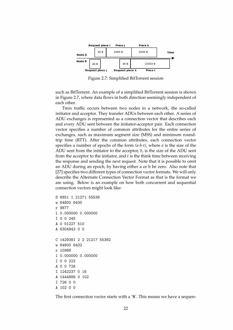
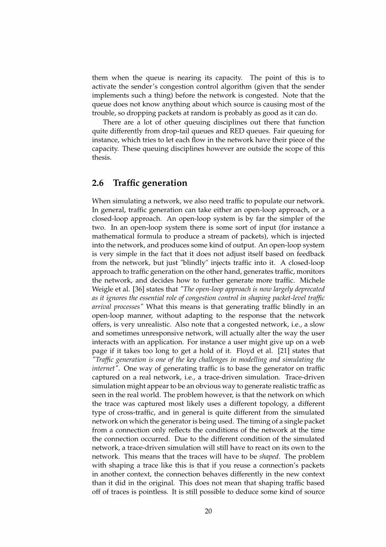
Figure 2.7: Simplified BitTorrent session

such as BitTorrent. An example of a simplified BitTorrent session is shownin Figure 2.7, where data flows in both direction seemingly independent ofeach other.

Tmix traffic occurs between two nodes in a network, the so-calledinitiator and acceptor. They transfer ADUs between each other. A series ofADU exchanges is represented as a connection vector that describes eachand every ADU sent between the initiator-acceptor pair. Each connectionvector specifies a number of common attributes for the entire series ofexchanges, such as maximum segment size (MSS) and minimum round-trip time (RTT). After the common attributes, each connection vectorspecifies a number of epochs of the form (a-b-t), where a is the size of theADU sent from the initiator to the acceptor, b, is the size of the ADU sentfrom the acceptor to the initiator, and t is the think time between receivingthe response and sending the next request. Note that it is possible to omitan ADU during an epoch, by having either a or b be zero. Also note that[27] specifies two different types of connection vector formats. We will onlydescribe the Alternate Connection Vector Format as that is the format weare using. Below is an example on how both concurrent and sequentialconnection vectors might look like:

S 6851 1 21271 55538w 64800 6430r 9877l 0.000000 0.000000I 0 0 245A 0 51227 510A 6304943 0 0

C 1429381 2 2 21217 55382w 64800 6432r 10988l 0.000000 0.000000I 0 0 222A 0 0 726I 1242237 0 16A 1444888 0 102I 726 0 0A 102 0 0

The first connection vector starts with a ’S’. This means we have a sequen-

22

tial connection. The rest of the first line is the start time (in microseconds),the number of epochs in the connection, and two identification numbers.In this case we have a sequential connection with one epoch, starting at6,851 ms (where 0 is the start of the simulation). The second line in a con-nection vector, starting with a ’w’, gives the window sizes of the initiatorand acceptor, respectively. The third line gives us a minimum RTT (in mi-croseconds), while the fourth line, which is the last line before the actualADUs, tells us the drop rate of the connection. For the actual ADUs, wehave lines starting with ’I’, which means an ADU sent from the initiator,and lines starting with ’A’ which means an ADU sent from the acceptor.The second and third field of these lines are two different types of waittimes. Note that one of these has to be zero. If the first one is non-zero, itmeans that we should wait an amount of time after sending our previousADU, before we send the next ADU. If the second one is non-zero, it meansthat we should wait an amount of time after receiving an ADU, before wesend the next one. In our first connection we first have an ADU of size 245sent from the initiator at time 0 (after the connection vector start). Upon re-ception of this ADU, the acceptor waits for 51,227 ms before replying with510 bytes, and then waits 6,3 seconds before closing the connection. Wesee that the last ADU is of size zero, this is a special placeholder ADU thatmeans we should close the connection. The second connection vector isquite similar to the first one. It starts with a ’C’, which tells us we havea concurrent connection. It specifies two numbers of epochs, as opposedto the one that the sequential connection specified. This is needed as theinitiator and acceptor are independent of each other, and may have a dif-ferent amount of epochs. The rest of the attributes preceding the ADUs,are the same for concurrent connections as for sequential connections. Theactual ADUs are self-explanatory. Note that the third field of each ADU isnever used, because the endpoints in a concurrent connection never waiton ADUs from its counterpoint. Also note that both ends close their con-nection.

2.7 The TCP evaluation suite

There is no doubt that the network research community could benefitfrom having a standardized set of test cases, to be used as an initialevaluation of new TCP extensions. Such an evaluation suite would allowresearchers proposing new TCP extensions to quickly and easily evaluatetheir proposed extensions through a series of well-defined, standard testcases, and also to compare newly proposed extensions with other proposalsand standard TCP versions. A common TCP evaluation suite has beenproposed by [17] and has been further developed by David Hayes [22] 1.

1The TCP evaluation suite is still a work in progress, meaning that some of the suitewill change, and some of the values have yet to be decided. The version cited is the latestversion released. There exists newer version. We have based our work on a snapshot of thesuite that we have acquired through private correspondence with David Hayes. There area few differences between the released version and the one we have. The differences will

23

In this chapter we will give a brief summary of the TCP evaluation suite asdescribed in the draft we received from Hayes.

2.7.1 Basic scenarios

There are a number of basic scenarios described in the evaluation suite:The data center, the access link, the trans-oceanic link, the geostationarysatellite, the wireless access scenario, and the dial-up link. All of thesescenarios are meant to model different networks as seen in the real world.

The access link scenario for instance, models a network connectingan institution, such as the University of Oslo, to an ISP. The central link(CL) itself has a very high bandwidth, and low delay. The leaf nodes onthe institution represent a group of users with varying amount of delayconnected to the institution’s network. Some of these users are perhaps oncampus, and are connected to the network through wireless access, thusgiving a high delay, while some of the users are directly connected to thenetwork by high-speed cabling, thus giving short delays.

The trans-oceanic link on the other hand, models the high capacity linksconnecting countries and continents to each other. The CL has a reallyhigh bandwidth, but also a high propagation delay because of the longdistances. The leaf nodes represent different types of users, with a varyingamount of delay, connected to the trans-oceanic link.

There are not only high-speed scenarios defined in the suite, there isalso the dial-up link scenario for instance. This models a network whereseveral users are connected to the same 64 kbps dial-up link. Scenarios likethese are reported as typical in Africa.

Each scenario is run for a set amount of time. The simulation runtime is different for each scenario. Some scenarios, like the access linkscenarios, have really high traffic and does not require as much time toachieve reasonable results, while others, like the dial-up link scenario,requires more time to achieve reasonable results. Every scenario also hasa warm-up period, in which measurements are not taken. This is to letthe network stabilize before taking measurements. The actual numbers arejust placeholder values in the version of the suite we have used, and aretherefore not described here. The values we have used in this thesis can beseen in the chapter about the ns-2 version of the suite.

Topology, node and link configurations

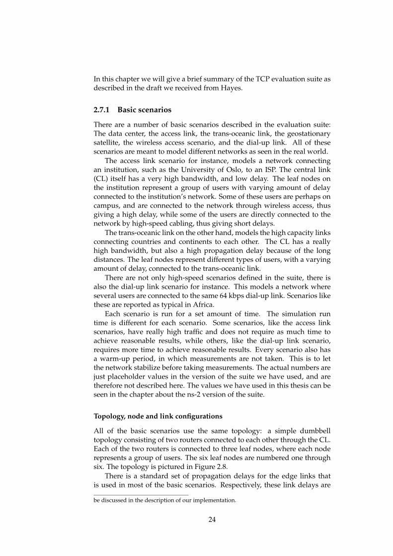
All of the basic scenarios use the same topology: a simple dumbbelltopology consisting of two routers connected to each other through the CL.Each of the two routers is connected to three leaf nodes, where each noderepresents a group of users. The six leaf nodes are numbered one throughsix. The topology is pictured in Figure 2.8.

There is a standard set of propagation delays for the edge links thatis used in most of the basic scenarios. Respectively, these link delays are

be discussed in the description of our implementation.

24

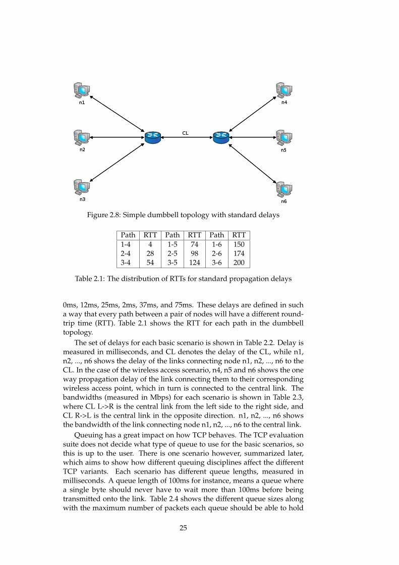
Figure 2.8: Simple dumbbell topology with standard delays

Path RTT Path RTT Path RTT1-4 4 1-5 74 1-6 1502-4 28 2-5 98 2-6 1743-4 54 3-5 124 3-6 200

Table 2.1: The distribution of RTTs for standard propagation delays

0ms, 12ms, 25ms, 2ms, 37ms, and 75ms. These delays are defined in sucha way that every path between a pair of nodes will have a different round-trip time (RTT). Table 2.1 shows the RTT for each path in the dumbbelltopology.

The set of delays for each basic scenario is shown in Table 2.2. Delay ismeasured in milliseconds, and CL denotes the delay of the CL, while n1,n2, ..., n6 shows the delay of the links connecting node n1, n2, ..., n6 to theCL. In the case of the wireless access scenario, n4, n5 and n6 shows the oneway propagation delay of the link connecting them to their correspondingwireless access point, which in turn is connected to the central link. Thebandwidths (measured in Mbps) for each scenario is shown in Table 2.3,where CL L->R is the central link from the left side to the right side, andCL R->L is the central link in the opposite direction. n1, n2, ..., n6 showsthe bandwidth of the link connecting node n1, n2, ..., n6 to the central link.

Queuing has a great impact on how TCP behaves. The TCP evaluationsuite does not decide what type of queue to use for the basic scenarios, sothis is up to the user. There is one scenario however, summarized later,which aims to show how different queuing disciplines affect the differentTCP variants. Each scenario has different queue lengths, measured inmilliseconds. A queue length of 100ms for instance, means a queue wherea single byte should never have to wait more than 100ms before beingtransmitted onto the link. Table 2.4 shows the different queue sizes alongwith the maximum number of packets each queue should be able to hold

25

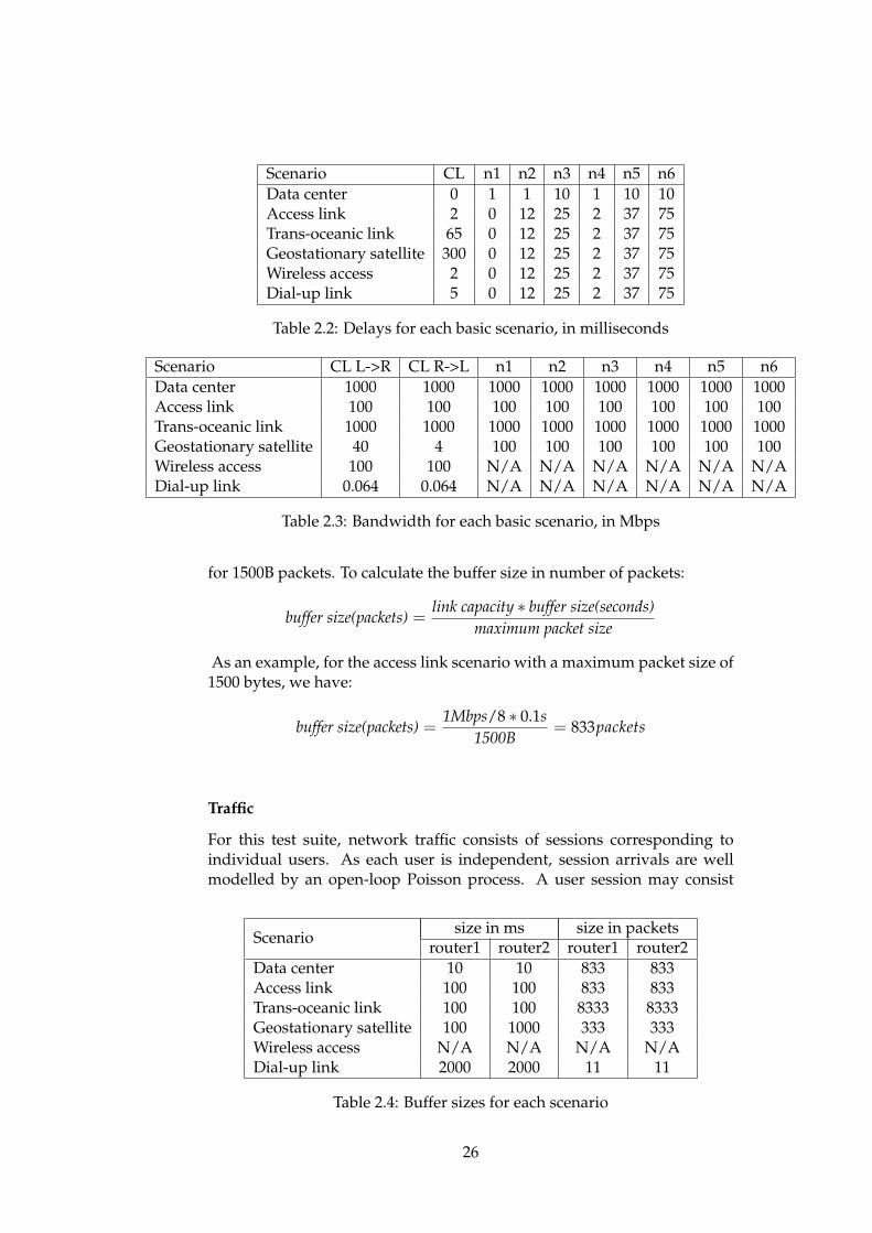
Scenario CL n1 n2 n3 n4 n5 n6Data center 0 1 1 10 1 10 10Access link 2 0 12 25 2 37 75Trans-oceanic link 65 0 12 25 2 37 75Geostationary satellite 300 0 12 25 2 37 75Wireless access 2 0 12 25 2 37 75Dial-up link 5 0 12 25 2 37 75

Table 2.2: Delays for each basic scenario, in milliseconds

Scenario CL L->R CL R->L n1 n2 n3 n4 n5 n6Data center 1000 1000 1000 1000 1000 1000 1000 1000Access link 100 100 100 100 100 100 100 100Trans-oceanic link 1000 1000 1000 1000 1000 1000 1000 1000Geostationary satellite 40 4 100 100 100 100 100 100Wireless access 100 100 N/A N/A N/A N/A N/A N/ADial-up link 0.064 0.064 N/A N/A N/A N/A N/A N/A

Table 2.3: Bandwidth for each basic scenario, in Mbps

for 1500B packets. To calculate the buffer size in number of packets:

buffer size(packets) =link capacity ∗ buffer size(seconds)

maximum packet size

As an example, for the access link scenario with a maximum packet size of1500 bytes, we have:

buffer size(packets) =1Mbps/8 ∗ 0.1s

1500B= 833packets

Traffic

For this test suite, network traffic consists of sessions corresponding toindividual users. As each user is independent, session arrivals are wellmodelled by an open-loop Poisson process. A user session may consist

Scenariosize in ms size in packets

router1 router2 router1 router2Data center 10 10 833 833Access link 100 100 833 833Trans-oceanic link 100 100 8333 8333Geostationary satellite 100 1000 333 333Wireless access N/A N/A N/A N/ADial-up link 2000 2000 11 11

Table 2.4: Buffer sizes for each scenario

26

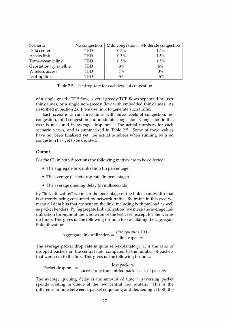
Scenario No congestion Mild congestion Moderate congestionData center TBD 0.5% 1.5%Access link TBD 0.5% 1.5%Trans-oceanic link TBD 0.5% 1.5%Geostationary satellite TBD 3% 6%Wireless access TBD 1% 3%Dial-up link TBD 5% 15%

Table 2.5: The drop rate for each level of congestion

of a single greedy TCP flow, several greedy TCP flows separated by userthink times, or a single non-greedy flow with embedded think times. Asdescribed in Section 2.6.1, we use tmix to generate such traffic.

Each scenario is run three times with three levels of congestion: nocongestion, mild congestion and moderate congestion. Congestion in thiscase is measured in average drop rate. The actual numbers for eachscenario varies, and is summarized in Table 2.5. Some of these valueshave not been finalized yet, the actual numbers when running with nocongestion has yet to be decided.

Output

For the CL in both directions the following metrics are to be collected:

• The aggregate link utilization (in percentage)

• The average packet drop rate (in percentage)

• The average queuing delay (in milliseconds)

By "link utilization" we mean the percentage of the link’s bandwidth thatis currently being consumed by network traffic. By traffic in this case wemean all data bits that are sent on the link, including both payload as wellas packet headers. By "aggregate link utilization" we mean the average linkutilization throughout the whole run of the test case (except for the warm-up time). This gives us the following formula for calculating the aggregatelink utilization:

Aggregate link utilization =throughput ∗ 100

link capacity

The average packet drop rate is quite self-explanatory. It is the ratio ofdropped packets on the central link, compared to the number of packetsthat were sent to the link. This gives us the following formula:

Packet drop rate =lost packets

successfully transmitted packets + lost packets

The average queuing delay is the amount of time a traversing packetspends waiting in queue at the two central link routers. This is thedifference in time between a packet enqueuing and dequeuing at both the

27

routers. As the link capacities of the edge links are always larger than thecapacity of the central link, we can assume that the queuing delay for theedge devices are 0, or close to 0. This gives us the following formula:

Queuing delay = (T2 − T1) + (T4 − T3)

where T2 is the timestamp on dequeuing from the first router, T1 isthe timestamp on enqueuing in the first router. T4 is the timestamp ondequeuing from the second router, and T3 is the timestamp on enqueuingin the second router. In addition to metrics collected for the central link,there are a number of metrics for each flow:

• The sending rate (in bps)

• Good-put (in bps)

• Cumulative loss (in packets)

• Queuing delay (in milliseconds)

The sending rate of a flow is the number of bits transmitted per second. Thisincludes both header and data, from both successfully transmitted packets,as well as packets that are eventually dropped. Good-put on the other hand,only measures the throughput of the original data. This means each andevery application level bit of data that is successfully transferred to thereceiver, excluding retransmitted packets and packet overhead. Cumulativeloss is the number of lost packets or the number of lost bytes. Queuingdelay is also measured for each flow, and is similar to the queuing delaydescribed for the central link. It is measured for each flow individually,and in addition to the central link queues, there may be other queues alongthe network which has to be taken into consideration.

2.7.2 The delay-throughput tradeoff scenario

Different queue management mechanisms have different delay-throughputtradeoffs. For instance, Adaptive Virtual Queue (AQM) gives low delay, atthe expense of lower throughput. The delay-throughput tradeoff (DTT)scenario investigates how TCP variants behave in the presence of differentqueue management mechanisms.

The tests in this scenario are run for the access link scenario. It is onlyrun for one level of congestion: moderate congestion when the queue size is100% of the bandwidth-delay product (BDP). The scenario is run five timesfor each queuing mechanism. When using drop-tail queues, the scenario isrun five times with queue sizes of 10%, 20%, 50%, 100%, and 200% of theBDP. For each AQM scenario (if used), five tests are run, with queue sizesof 2.5%, 5%, 10%, 20%, and 50% of the BDP.

For each scenario, the output should be two graphs. One shows theaverage throughput as a function of average queuing delay, while the othergraph shows the packet drop rate as a function of average queuing delay.

28

2.7.3 Other scenarios

We have described the most basic scenarios in detail in the precedingsections, and will briefly mention the rest of the scenarios in this section,so that the reader can get an impression of the range of tests that isincluded in the suite. There is one test named "Ramp up time". Thistest aims to determine how quickly existing flows make room for newflows. The "Transients" scenario investigates the impact of sudden changesin congestion. This scenario observes what happens to single long-livedTCP flow as congestion suddenly appears or disappears. One scenarioaims to show how the tested TCP extension impacts standard TCP traffic(where the standard TCP variant is defined to be NewReno). This scenariois run twice: once with only the standard TCP variant, and once wherehalf the traffic is generated by a standard TCP variant, and the otherhalf is generated by the TCP extension to be evaluated. The results ofthese two runs are compared. The "Intra-protocol and inter-RTT fairness"scenario aims to measure bottleneck bandwidth sharing among flows usingthe same protocol going through the same routing path, but also thebandwidth sharing among flows of the same protocol going through thesame bottleneck, but different routing paths. Finally, we have the "multiplebottlenecks" scenario where the relative bandwidth for a flow traversingmultiple bottlenecks is explored.

2.7.4 The state of the suite

A few words on the state of the evaluation suite are necessary. The TCPevaluation suite is the outcome of a "round-table" meeting in 2007 on TCPevaluation, and is described by Floyd et al. [17]. While the idea of creatinga standardized test suite to evaluate TCP is a good one, there are a numberof details that were not really thought through in the beginning. DavidHayes picked up on the suite eventually and started work on improvingthe suite. The evaluation suite has been constantly updated while we havebeen working on this thesis. We have been working on a snapshot of thesuite which we received from Hayes personally. At the moment, the projectis at a halt because of a number of issues with the suite. Unfortunately wedid not know this when we started working on this thesis. This section isbased on conversations with Hayes.

The main problem with the suite is the way that congestion is measured.Each test defines a level of congestion measured in average drop rate. Thismeans that traffic (from tmix) will have to be scaled in such a way that thetest reaches a target loss rate. For instance, the target loss rate for the accesslink basic scenario with moderate congestion is 1.5%.

The problem with doing it this way is that if the network is alwayscongested, packets will be retransmitted, which adds to the traffic, andcongests the network further. After a while a network collapse will occur.This is a state in which hardly any traffic gets through the network becauseof the enormous amount of traffic. The evaluation suite defines an averagedrop rate for each scenario, which means that there will have to be quite

29

a lot of traffic, and that the network is always on the verge of collapsing.Figure 2.9 shows this network collapse with the three levels of congestionthat each basic scenario defines marked on the curve. The network at thispoint is not very stable.

Tmix traffic also makes defining congestion by an average drop ratedifficult. This is because the traffic constantly changes along the run ofa simulation. At times there might be high peaks of traffic that is quitedifferent to the rest of the traffic. For short simulations, it is possible to finda scale for tmix, so that the average drop rate of the run matches the targetrate. However if the simulation is run for a long time, it is not possibleto find such a scale, because at some point along the simulation there willmost likely be a peak of traffic so high that the network will collapse andnot recover from it. Avoiding the peak by setting the scale lower will resultin the average drop rate being too low. According to Hayes, the suitewill have to go through some drastic changes when it comes to definingcongestion levels before the suite can be used for what it was originallyintended: evaluation of TCP extensions.

The suite defines congestion by a target drop rate, but it also specifiesthat the output of each test should be the average drop rate of the centrallink. This in itself is quite weird, because if the drop rate metric doesnot match the target drop rate, then the test is not implemented as it wasspecified in the suite. This is also quite difficult when it comes to runningthe suite with different TCP variants, because when different TCP variantsare used, different drop rates are measured, and all of them cannot meetthe target drop rate. While the suite is a bit unclear about this, it is possibleto compare the relative loss between different TCP variants as long as a"default" variant has been decided. The scale and target drop rate could bebased on the "default" variant.

Through talks with Hayes we now know that the evaluation suite in itscurrent state cannot be used as a tool to evaluate TCP; however there is noreason while the test cases cannot be used to compare network simulatorsas long as a proper scale is set, and the network does not collapse.

30

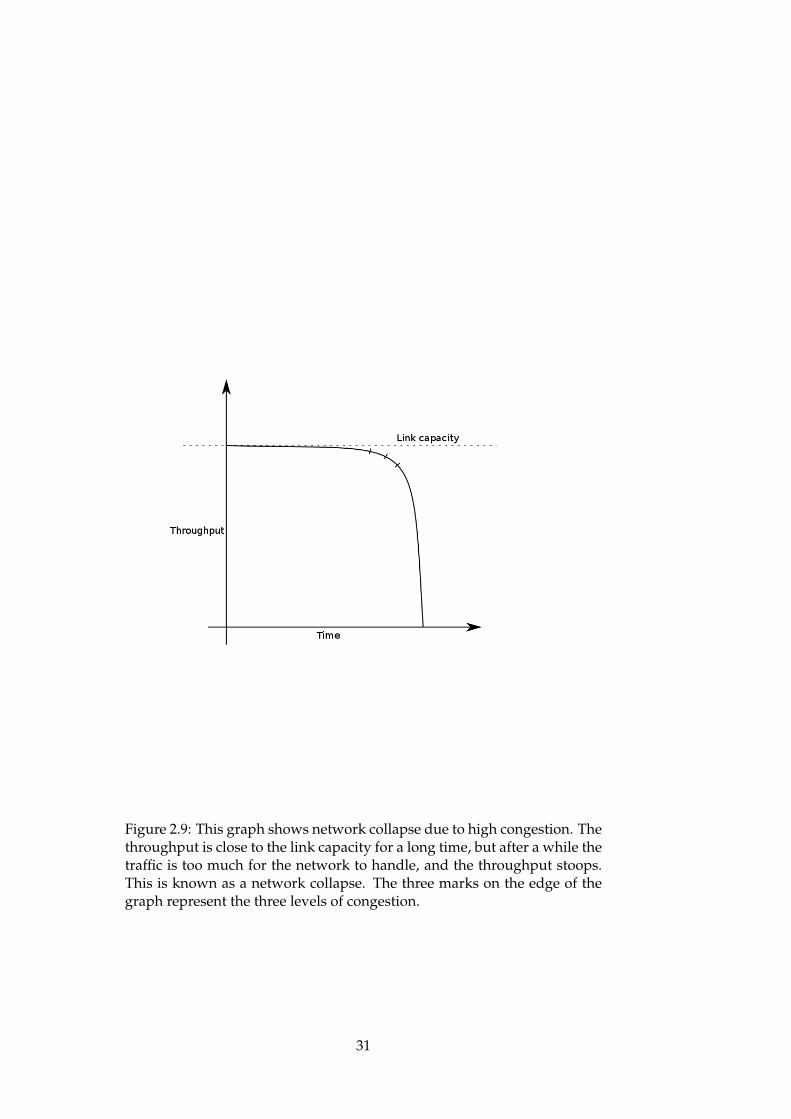
Figure 2.9: This graph shows network collapse due to high congestion. Thethroughput is close to the link capacity for a long time, but after a while thetraffic is too much for the network to handle, and the throughput stoops.This is known as a network collapse. The three marks on the edge of thegraph represent the three levels of congestion.

31

32

Chapter 3

The TCP evaluation suiteimplementation

In this chapter we will go through the TCP evaluation suite implementationfor each of three simulators. The ns-2 version of the TCP evaluation suite[9] is available online and has been developed by David Hayes. The draftwhere the TCP evaluation suite is described will hereby be referred to asthe draft. In this thesis we have used the TCP evaluation suite as a basicset of test cases that we can use to compare network simulators. Wheneverthe ns-2 version of the suite differs from the draft, we have tried to makeour simulations as close to the ns-2 version as possible to make the resultscomparable.

As mentioned in the section about the draft, the TCP evaluation suite isnot yet applicable as a tool to evaluate TCP due to a number of problems.The same goes for the ns-2 version of it. None the less, the ns-2 versionof the tool should still be useful for us to evaluate and compare networksimulators.

3.1 ns-2

This section will briefly introduce the ns-2 network simulator, as well asdescribe the ns-2 version of the TCP evaluation suite, with focus on thedifferences between the draft and the ns-2 implementation of it.

3.1.1 Introduction

ns-2 is an event-driven simulator, which has been proved useful instudying the dynamic nature of communication networks [23]. Due toits flexibility and modular nature, ns-2 quickly became a success in thenetwork research community after its release in 1989. For many years thens-2 network simulation tool has been the de-facto standard for academicresearch into networking protocols and communication methods accordingto [35], and a simple search on the web, both on Google[4] and on the ACMDigital Library[1], gives an enormous amount of results for ns-2 comparedto other network simulators.

33

ns-2 consists of two key languages: C++ and Object-oriented ToolCommand Language (OTcl). The internal mechanism of each module iswritten in C++, while OTcl is used to assemble and configure modules, aswell as to schedule events.

ns-2 has a vast number of simulation models available online, andmost research requires models which are beyond the scope of the built-in ns-2 modules. Incorporating these modules into ns-2 requires profoundunderstanding of ns-2 architecture, and may feel like daunting task for ns-2beginners. ns-2 has been criticized of being difficult to use, which is one ofthe reasons we see alternative network simulators today. Issariyakul et al.[23] says that "...the formal documentation of ns-2 is mainly written as a referencebook, and does not provide much information for beginners. The lack of guidelinesfor extending ns-2 is perhaps the greatest obstacle, which discourages numerousresearchers from using ns-2".

3.1.2 The evaluation suite implementation

The ns-2 evaluation suite follows the draft described in Section 2.7 asfar as possible. The main parts of the ns-2 version are implemented asdescribed in the draft, but there are still several minor differences betweenthe draft and the actual ns-2 implementation. The reason for why thens-2 implementation differs from the draft is because it is currently awork in progress and therefore constantly changes. The snapshot thatwe have of the draft probably differs from the snapshot of the draft thatthe ns-2 implementation is based on. The ns-2 version of the suite can bedownloaded from http://caia.swin.edu.au/ngen/tcptestsuite/tools.html.The connection vector files used can also be downloaded from the samelocation.

The suite is implemented in a very modular way, making it easy toadd new tests to the implementation, as well as adding new TCP variantsto it. The ns-2 implementation does not include every test described inthe draft, but includes the following ones: the basic scenarios, the delay-throughput tradeoff scenario, impact on standard TCP, ramp-up time andmultiple bottlenecks.

Every scenario in the ns-2 implementation uses the same set ofconnection vector files. To change the amount of traffic, they scale thetraffic generated by tmix. This means that the time at which a connection isscheduled to start is time * scale instead of just time. This makes it possibleto either spread out the connections, or to concentrate them. We havefollowed this example and added the possibility of scaling traffic in ns-3, and we have also built in this functionality in our OMNeT++ versionof tmix. Each basic scenario is run three times with three different levelsof congestion: uncongested, mild congestion, and moderate congestion.The draft does not specify a value for the uncongested run. In the ns-2 version, uncongested is twice the scale of mild congestion. For thedelay-throughput tradeoff scenario, the level of traffic is specified to havemoderate congestion when the buffer size is 100% of the bandwidth-delayproduct for a 100ms flow. Table 3.1 contains all the scales used in ns-2.

34

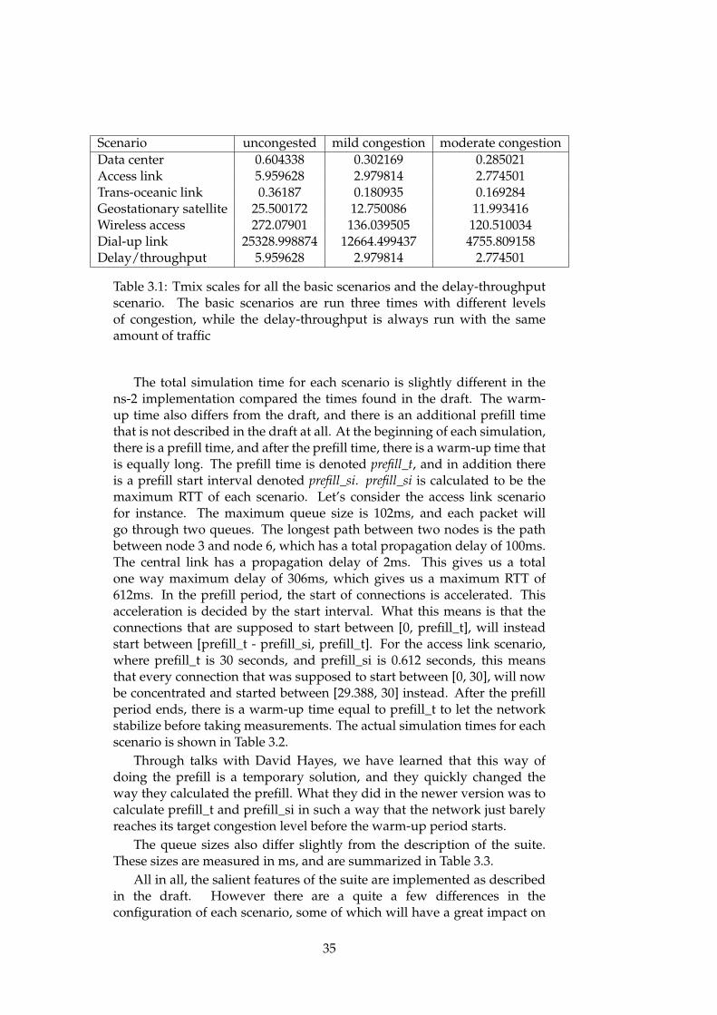
Scenario uncongested mild congestion moderate congestionData center 0.604338 0.302169 0.285021Access link 5.959628 2.979814 2.774501Trans-oceanic link 0.36187 0.180935 0.169284Geostationary satellite 25.500172 12.750086 11.993416Wireless access 272.07901 136.039505 120.510034Dial-up link 25328.998874 12664.499437 4755.809158Delay/throughput 5.959628 2.979814 2.774501

Table 3.1: Tmix scales for all the basic scenarios and the delay-throughputscenario. The basic scenarios are run three times with different levelsof congestion, while the delay-throughput is always run with the sameamount of traffic

The total simulation time for each scenario is slightly different in thens-2 implementation compared the times found in the draft. The warm-up time also differs from the draft, and there is an additional prefill timethat is not described in the draft at all. At the beginning of each simulation,there is a prefill time, and after the prefill time, there is a warm-up time thatis equally long. The prefill time is denoted prefill_t, and in addition thereis a prefill start interval denoted prefill_si. prefill_si is calculated to be themaximum RTT of each scenario. Let’s consider the access link scenariofor instance. The maximum queue size is 102ms, and each packet willgo through two queues. The longest path between two nodes is the pathbetween node 3 and node 6, which has a total propagation delay of 100ms.The central link has a propagation delay of 2ms. This gives us a totalone way maximum delay of 306ms, which gives us a maximum RTT of612ms. In the prefill period, the start of connections is accelerated. Thisacceleration is decided by the start interval. What this means is that theconnections that are supposed to start between [0, prefill_t], will insteadstart between [prefill_t - prefill_si, prefill_t]. For the access link scenario,where prefill_t is 30 seconds, and prefill_si is 0.612 seconds, this meansthat every connection that was supposed to start between [0, 30], will nowbe concentrated and started between [29.388, 30] instead. After the prefillperiod ends, there is a warm-up time equal to prefill_t to let the networkstabilize before taking measurements. The actual simulation times for eachscenario is shown in Table 3.2.

Through talks with David Hayes, we have learned that this way ofdoing the prefill is a temporary solution, and they quickly changed theway they calculated the prefill. What they did in the newer version was tocalculate prefill_t and prefill_si in such a way that the network just barelyreaches its target congestion level before the warm-up period starts.

The queue sizes also differ slightly from the description of the suite.These sizes are measured in ms, and are summarized in Table 3.3.

All in all, the salient features of the suite are implemented as describedin the draft. However there are a quite a few differences in theconfiguration of each scenario, some of which will have a great impact on

35

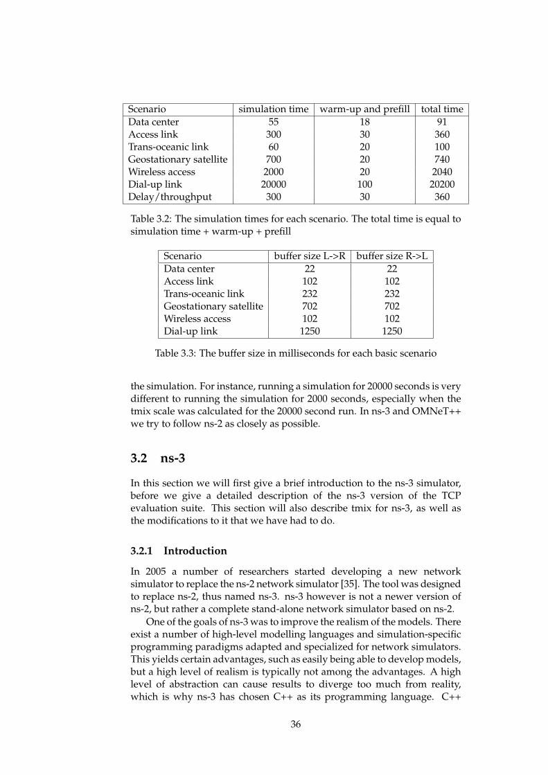
Scenario simulation time warm-up and prefill total timeData center 55 18 91Access link 300 30 360Trans-oceanic link 60 20 100Geostationary satellite 700 20 740Wireless access 2000 20 2040Dial-up link 20000 100 20200Delay/throughput 300 30 360

Table 3.2: The simulation times for each scenario. The total time is equal tosimulation time + warm-up + prefill

Scenario buffer size L->R buffer size R->LData center 22 22Access link 102 102Trans-oceanic link 232 232Geostationary satellite 702 702Wireless access 102 102Dial-up link 1250 1250

Table 3.3: The buffer size in milliseconds for each basic scenario

the simulation. For instance, running a simulation for 20000 seconds is verydifferent to running the simulation for 2000 seconds, especially when thetmix scale was calculated for the 20000 second run. In ns-3 and OMNeT++we try to follow ns-2 as closely as possible.

3.2 ns-3

In this section we will first give a brief introduction to the ns-3 simulator,before we give a detailed description of the ns-3 version of the TCPevaluation suite. This section will also describe tmix for ns-3, as well asthe modifications to it that we have had to do.

3.2.1 Introduction

In 2005 a number of researchers started developing a new networksimulator to replace the ns-2 network simulator [35]. The tool was designedto replace ns-2, thus named ns-3. ns-3 however is not a newer version ofns-2, but rather a complete stand-alone network simulator based on ns-2.

One of the goals of ns-3 was to improve the realism of the models. Thereexist a number of high-level modelling languages and simulation-specificprogramming paradigms adapted and specialized for network simulators.This yields certain advantages, such as easily being able to develop models,but a high level of realism is typically not among the advantages. A highlevel of abstraction can cause results to diverge too much from reality,which is why ns-3 has chosen C++ as its programming language. C++

36

is a powerful programming language with many possibilities. One ofthe main reasons for going with C++, is because most protocol stackimplementations are implemented in C, thus making them easier toincorporate into ns-3 simulations. Another reason to make a new stand-alone network simulator instead of making a new version of ns-2 isbecause of software maintenance. ns-3 (as well as ns-2) is not commerciallysupported, but open-source. This means that a lot of different people arecontributing to the code-base. One of the main points of ns-3 has been toenforce a strict coding standard, as well as a code review process and atest infrastructure to ensure a high quality in all software added to the tool.This was not the case with ns-2 which made the tool grow considerablyover time and led users to lose confidence in the results.

ns-3 models several objects from the real world. Below are a fewexamples of the models in ns-3:

• A Node represents end-points as well as routers, hubs and switches inthe network. There is no difference between the nodes in a network.Computation power for instance is not taken into consideration.Hardware is also not a part of the model.

• A Device represents the physical device that connects a node to acommunication channel. A switch for instance, may have severalEthernet network devices, while a wireless access point includes an802.11 device on which packets may arrive wirelessly.

• Communication channels connect to network devices and representa medium on which data may be transmitted. A communicationchannel could represent a fibre-optic link, a twisted pair cable, or thewireless spectrum for wireless communication.

• Communication protocols include common Internet protocols such asEthernet, 802.11, TCP or UDP for instance. Many of the typicalInternet protocols found in the TCP/IP stack are part of the ns-3 core.In ns-3 it is also possible to run real-world protocol stacks (such as theones found in Linux or in FreeBSD) through the network simulationcradle (NSC).

• Network packets represent packets being sent on the network. Eachpacket usually contains one or more protocol headers, as well as apayload of data that depends on the application being used.

• Applications are modelled as well. What is the point of buildinga network if there is no traffic? The applications found in ns-3are typically quite simple, for instance the OnOffApplication is anapplication that will send bursts of data at a given time interval.

Modelling elements from the real world is obviously necessary tocreate a simulator. In addition to the model itself, ns-3 includes severalpractical solutions which assist the user in both execution and analysis of asimulation: attributes, helper objects, and trace sources.

37

In most cases the user will have to change the behaviour of some of themodels used in a simulation. Each model is defined by several Attributes.These attributes can easily be set by the user through public functionsprovided by the objects. The PointToPointNetDevice class for instance canbe used with its default values, however if the user wants to change thebehaviour of this device, that is easily done by functions provided by theclass. ns-3 forces all models to be implemented with this attribute system.

Helper objects are used in ns-3 to assist the user in creating the simulationscript. Consider a very common task in any network simulation:connecting two nodes to each other by a common communication channel.To do this, one typically needs to perform a number of core operations.First of all, we need at least two nodes, where each of the nodes has theirown network device to which we can connect the channel. Each of thedevices will have to be assigned a MAC address for the link-layer protocolto function properly. The nodes will need a protocol stack (such as theIP/TCP protocol stack) installed etc. This is a very common task, andns-3 has a system to help perform such tasks more easily: helper objects.The point of these objects is to have the user quickly and easily performcommon tasks without having to dig into the details. An example of ahelper is the PointToPointHelper class. When using the PointToPointHelper,it is possible to set attributes for both the device and channel easily,such as the bandwidth and delay of the channel, and the maximumtransmission unit of the device. Once these details have been decided, thePointToPointHelper will be installed on a group of nodes. Each of the nodesincluded in this group will get a PointToPointNetDevice installed, as well asa PointToPointChannel connecting every pair of nodes. The same goes forsetting up a node with the TCP/IP protocol stack. There is a helper namedInternetStackHelper which will install the entire stack on a group of nodes.

The goal of any simulation is to generate data that can later be analysedand presented. Trace sources facilitate the logging of data during anexecution of a simulation. Trace sources are entities that signal certainevents whenever they happen during the course of a simulation. The tracesources are not useful on their own, but must be connected to other piecesof code that actually do something useful with the information providedby the trace source. The entities that consume trace information are calledtrace sinks. Trace sources generate events, while trace sinks consume them.When a trace sink expresses interest in receiving trace events, it adds acallback to the list of callbacks held by the trace source. Whenever the tracesource notices an event happening, it goes through this list of callbacks,and calls every trace sink registered. It is up to each and every trace sinkto decide what they want to do when an event happens. There are severalpre-defined packages in the core of ns-3 that use trace sources to generatedata. For instance, there is a package that outputs PCAP1 files based on aset of difference trace sources, and there is another package flowmon that

1PCAP [6] (packet capture) consists of an application programming interface forcapturing network traffic. Monitoring software may observe the network and output everypacket that passes through the network. These packets are printed in a PCAP file and canlater be analysed using software such as Wireshark or tcpdump.

38

generates statistics on each flow in the simulation. Through the use of acombination of both pre-defined packages and custom made trace sinks,the user should easily be able to generate interesting data.

3.2.2 Tmix for ns-3

The core of ns-3 contains a number of basic traffic generators, but nothinglike tmix, which is needed to make our ns-3 version of the evaluation suitecomparable to the ns-2 version. ns-3 tmix[13] was developed by a group ofstudents in a Google Summer of Code project in 20112.

The release of the tmix traffic generator for ns-3 was a very welcomeaddition to the simulator. However the generator is not perfect, thesource code is filled with comments about missing functionality and weakimplementation details that were to be fixed, but unfortunately never werebefore the release of it. As a result of this, we have had to do a bit of work toget the generator to do what we wanted. In addition to the traffic generatorbeing a bit buggy, it is also completely lacking any documentation.

Tmix for ns-3 was originally developed for version 3.10 in 2011. Severalnew versions of ns-3 have been released since then. In version 3.13 theentire source code structure was redesigned. This made it necessary toreorganize the source code of tmix as well to adhere to the new ns-3structure. The traffic generator consists of two modules: the tmix module,and the delaybox module. In the 3.10 version they were residing in foldersthat were removed in ns-3.13. To make it compile with ns-3.13, we madetmix and delaybox their own stand-alone modules. To make this work wehad to change a lot of the header includes as many of the modules thatthe older version depended on were either not existing anymore, mergedwith other modules, or moved. In addition to fixing the dependencies, wealso had to reorganize the code of tmix and delaybox into the new folderstructure that ns-3.13 introduced. This means splitting the module, helperclasses, documentation, examples and tests in their own folders. When wesubmitted the new ns-3.13 version of tmix, they released ns-3.14, whichmade tmix crash once again. Luckily, this was just a matter of renaming afew constants.

In ns-2, they have extended the functionality of tmix to make it moresuitable for the TCP evaluation suite. They have, for instance, created anadditional parameter ’m’ that defines the maximum segment size (MSS) ofeach connection vector. To do this in ns-3, we first had to extend the parserso that it read the ’m’ parameter, and then stored it in the connection vectorstructure together with the other parameters. When a tmix applicationis started, it creates a socket to communicate through. We modified theconfiguration of this socket so that the MSS was set correctly.

In ns-2, they have also extended the functionality of tmix so that it ispossible to scale the traffic. We have done the same for ns-3 tmix. This wasjust a matter of setting the time at which a connection is due to start to "time* scale" instead of just "time".

2Google Summer of Code is a global program that offers students the possibility ofworking on an open-source project together with a mentor.

39

Tmix includes a set of helper functions included in the file tmix-topology.cc. This makes it very easy to create a dumbbell topologywhere the nodes use the tmix traffic generator without having to diginto the implementation details. The problem with this helper was thateach acceptor expected to only communicate with one initiator. In ourevaluation suite however, every node on the left side communicates withevery node on the right side.

The way that the communication was set up was not very intuitive.Tmix traffic is always set up between an initiator and acceptor. In the ns-3 version of tmix, when the initiator started a new connection, it wouldgenerate a new port for that connection. It would not use the new port tobind a new socket itself however. The initiator would call a function at theacceptor, declaring that the initiator would soon connect to the given port.The acceptor would then listen to a connection on that port, and accept onlythe first connection. The problem occurred when we tried to let one nodeact as an acceptor in several initiator/acceptor pairs. This was becausethe initiators allocated port numbers on their own. These port numbersconflicted with the port numbers that the other initiators allocated.

The best solution would be to completely redesign this, and handlethe client/server communication a little differently. Instead of letting theinitiators allocate ports for the server, they could rather allocate ports forthemselves. The server could listen for connections on the same portthroughout the entire run of the simulation, and create a thread for eachincoming connection to handle it. This should be much simpler and moreintuitive as well. We have chosen an alternate solution, which is easier toimplement, but is really just a quick fix for the problem.

The tmix-topology helper sets up two routers and a pair of nodescommunicating in the initialization phase. It has a function named"NewPair" that adds an extra pair of nodes: one on the left side, and one onthe right side. This function sets up the nodes, as well as a tmix applicationthat generates the traffic. We have created an additional function named"AddAdditionalApplications". This does exactly the same as the NewPairfunction except for actually creating two new nodes. Instead it takes apair of already existing nodes as input and creates a tmix application inboth of them that communicate with each other. To make sure that the portnumbers do not conflict with each other, a range of port numbers is set inthe application. The port allocator will start at the lowest port available forthe application, and never go above the port number limit.

All in all, the tmix version that we have received has been of great helpin this thesis, although at times frustrating to use because of the lack ofdocumentation.

3.2.3 The evaluation suite implementation

The ns-3 TCP evaluation suite has been implemented according to thedescription in section 2.7. Where the ns-2 version of the suite differs fromthe description of the suite, we have chosen to make our version as close tothe ns-2 version as possible to make the results comparable. All the files of

40

the suite are bundled together in a folder named eval which is located in theexamples folder of ns-3). This means that the TCP evaluation suite in ns-3 isimplemented as an ns-3 example. This does not really have an impact onthe suite, only on how the suite is compiled. For instructions on how to usethe evaluation suite, see Appendix A.

Architecture

The test suite consists of a few components. For every topology there isa file building that topology. For instance there is a file for the dumbbelltopology, named dumbbell.cc (and its header file dumbbell.h). In additionto the topology, there is another file (named after the scenario it describes)that configures a scenario. For instance there is a file named basic-scenario.cc that configures each of the basic scenarios. This means choosingthe correct topology, choosing the bandwidth and delay of each link, andsetting up the traffic and so on. The utils folder contains a few utilities,such as the timestamp-tag, which makes it possible to attach a timestampto a packet, and a parser that can be used to parse simulation output. Toeasily use the evaluation suite, a main script has been included, tcp-eval.sh.This script accepts simple commands such as "./tcp-eval.sh accessLink" tostart the access link scenario, as well as run the analysis script when thesimulation is finished. This hides the implementation from the user.

Topology and protocol stack

The topology used in the simulation depends entirely on the scenario to berun. Most of the scenarios in the evaluation suite use a typical dumbbelltopology. The basic setup for most of our tests, is described in a file nameddumbbell.cc, which sets up a dumbbell topology using the TmixTopologyclass as help. The TmixTopology class is a sort of helper to quickly helpthe user setting up a standard topology for testing purposes. The topologyalways contains a central link, and it is possible to create pairs of nodesin addition to the central link, where one node is on the left side, and onenode is on the right side. These nodes are all properly set up using theInternetStackHelper so that every node has a complete stack of protocols.In addition to the normal nodes and routers, the topology contains aDelayBox, which is required for tmix.

As our link-layer protocol, we use the very simple Point-to-PointProtocol (PPP). This is a very basic protocol that hardly contains anyfunctionality at all. The reason for using such a simple protocol is to ensurethat we do not fool TCP into thinking the network is congested. TCPwill always treat lost packets as lost because of congestion, and as suchwill adjust its sending rate to avoid further congestion. We want to avoidthis happening because of random errors in the link and physical layer,therefore we have this very simple link-layer protocol together with PPPchannels that never drop packets, nor generate bit-errors.

The queues used for each device are all of the type DropTailQueue formost scenarios. The queue sizes are specified in the TCP evaluation suite,

41

but we use the values presented in the chapter about the ns-2 version ofthe suite. The topology builder class will take queue size in milliseconds asinput, but will calculate the actual size in number of packets. This is doneusing the following formula:

queue size =C ∗ T

M∗ 1

8

where C is the central link’s capacity, T is the maximum wait time for apacket, and M is the maximum packet size.

The network-layer protocol used is IPv4. The only other option reallywould be IPv6, but choosing either one should not make an impact onthe simulation. The packets will be able to find their way through thenetwork either way, and the packet overhead is not that different betweenthe versions anyway. The protocol header in IPv6 is slightly larger thanin IPv4, but this should not make a significant impact on the simulation,and even if it was significant, we use IPv4 for all three simulators. Thenetwork is configured in such a way that every endpoint on the left sidehas addresses of the form 10.1.0.0/16. The endpoints on the right side haveaddresses of the form 10.2.0.0/16, while the routers have addresses fromthe network mask 10.3.0.0/16. This means that our network is split intothree subnets. The reason for this is that it makes it very easy to decide inwhich direction a packet is heading. If it is heading towards an addressthat starts with 10.1 for instance, it is heading towards the left side of thenetwork. If it is heading towards an address that starts with 10.2, then it isheading towards the right side.

ns-3 has several TCP variants built-in: TCP with no congestion control,Tahoe, Reno, and NewReno. We have chosen to use Reno and NewRenoin our simulations. TCP with no congestion control is very out-dated, as isTCP Tahoe. In addition to the built-in variants, ns-3 has the possibility ofrunning real-world protocol stacks through the Network Simulation Cradle(NSC) [8]. NSC is a framework which allows real world TCP/IP stacks tobe used inside a network simulator. ns-3 currently only supports the Linuxstacks. The downside of running real-world protocol stacks, as opposedto running built-in protocol stacks, is that the real-world ones are muchmore complex, thus slowing down the simulations by quite a bit. We triedto run CUBIC through NSC in ns-3. Without changing anything but theprotocol stack however, the simulation crashes after running for a very longtime. Only the shortest running test (the dial-up link scenario) was able tocomplete using NSC, and this took quite a long time compared to runningthe built-in version.

Traffic generation

When we began working on this thesis, tmix was not yet released. Wewere looking for alternative ways to generate traffic that would looksomewhat like the traffic that tmix generates in ns-2. In ns-3 there are afew basic applications that generate traffic, including simple bulk transferapplications, on-off applications (which send bursts of data at a given time

42

interval) etc. These are too simple and too predictable to be comparable totmix.

We found a tool based on the Poisson Pareto Burst Process (PPBP) [16]for generating Internet traffic. The PPBP traffic generator aims to createa generator that matches certain attributes from real-life IP networks. Weused this traffic generator for a while, and even though it is more realisticthan the simple applications in the ns-3 core as it is less predictable, it is stilldifficult to configure the generator in such a way that the traffic reassemblestraffic as generated by tmix.

During the summer 2012, tmix for ns-3 was released and we decidedto use it. Traffic is described through a series of connection vector files,defined as a part of the topology definition. Each node on the left sidecommunicates with every node on the right side and vice versa. This meansthat there are nine pairs of communicating nodes, and for each one there isa connection vector file specifying the traffic. All traffic flows through thecentral link. This is the same as for ns-2.

We use the same connection vector files that are used in ns-2. Theproblem however is that they are in the original connection vector format(as described in the ns-2 manual [27]), while tmix for ns-3 only supportsthe newer alternate connection vector format. Some time was spent tryingto make the parser in ns-3 tmix compatible with both formats, but throughprivate correspondence with Michele Weigle (who has been part of the tmixproject for both ns-2 and ns-3) we have received a script that converts fromthe original format to the alternate format. Since the connection vector filesin the ns-2 version of the suite contains the additional ’m’ parameter, wehave extended the script to include this parameter as well.

Collecting and presenting statistics

The point of any simulation is to collect data and to present them in ameaningful way. For a description of the metrics to be collected see section2.7. As mentioned in section 3.2.1, ns-3 has several trace sources availablethat will notify trace sinks whenever certain events occur. There are severalpre-existing packages that produce statistics in ns-3. We have implementedthis part of the simulation twice. We will describe both our solutions as theyboth give the correct results, however, the first solution is more complex,slows down the simulation, as well as requiring quite a lot of disk space,which is why we decided to redo it.

One of the reasons for the poor design in our first attempt was becausewe did not fully understand the tracing system in ns-3. This made us relymostly on the pre-defined tracing packages. To generate our results, wemade every PPP net device in the simulation generate pcap files. The pcapfiles were then parsed with the parser found in the utils folder. To parse thepcap files we used the libpcap package for developers. This contains a lotof functions and structures to ease the process of parsing pcap files. Theparser is best described in pseudo code:

f o r ( every packet in the pcap f i l e )

43

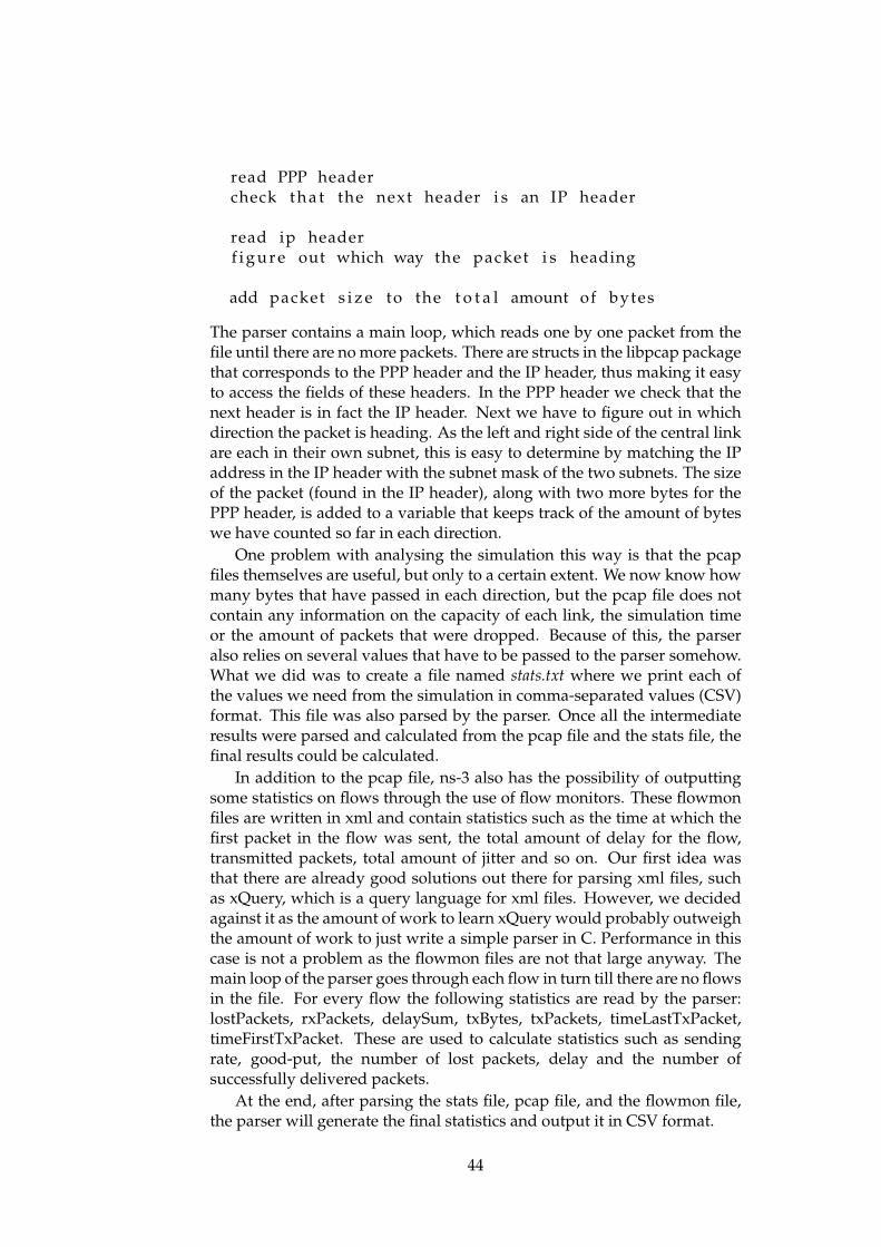
read PPP headercheck t h a t the next header i s an IP header

read ip headerf i g u r e out which way the packet i s heading

add packet s i z e to the t o t a l amount of bytes

The parser contains a main loop, which reads one by one packet from thefile until there are no more packets. There are structs in the libpcap packagethat corresponds to the PPP header and the IP header, thus making it easyto access the fields of these headers. In the PPP header we check that thenext header is in fact the IP header. Next we have to figure out in whichdirection the packet is heading. As the left and right side of the central linkare each in their own subnet, this is easy to determine by matching the IPaddress in the IP header with the subnet mask of the two subnets. The sizeof the packet (found in the IP header), along with two more bytes for thePPP header, is added to a variable that keeps track of the amount of byteswe have counted so far in each direction.

One problem with analysing the simulation this way is that the pcapfiles themselves are useful, but only to a certain extent. We now know howmany bytes that have passed in each direction, but the pcap file does notcontain any information on the capacity of each link, the simulation timeor the amount of packets that were dropped. Because of this, the parseralso relies on several values that have to be passed to the parser somehow.What we did was to create a file named stats.txt where we print each ofthe values we need from the simulation in comma-separated values (CSV)format. This file was also parsed by the parser. Once all the intermediateresults were parsed and calculated from the pcap file and the stats file, thefinal results could be calculated.

In addition to the pcap file, ns-3 also has the possibility of outputtingsome statistics on flows through the use of flow monitors. These flowmonfiles are written in xml and contain statistics such as the time at which thefirst packet in the flow was sent, the total amount of delay for the flow,transmitted packets, total amount of jitter and so on. Our first idea wasthat there are already good solutions out there for parsing xml files, suchas xQuery, which is a query language for xml files. However, we decidedagainst it as the amount of work to learn xQuery would probably outweighthe amount of work to just write a simple parser in C. Performance in thiscase is not a problem as the flowmon files are not that large anyway. Themain loop of the parser goes through each flow in turn till there are no flowsin the file. For every flow the following statistics are read by the parser:lostPackets, rxPackets, delaySum, txBytes, txPackets, timeLastTxPacket,timeFirstTxPacket. These are used to calculate statistics such as sendingrate, good-put, the number of lost packets, delay and the number ofsuccessfully delivered packets.

At the end, after parsing the stats file, pcap file, and the flowmon file,the parser will generate the final statistics and output it in CSV format.

44

The parser was our first attempt at generating statistics for ns-3.However, as we learned more about the simulator, and especially learnedmore about the tracing system, this seemed like a much simpler and moreelegant way of handling statistics. The trace sources that are generatedby the queues are especially useful. Each queue will report each enqueue,dequeue, and drop event. One way to connect trace sinks to trace sourcesis through the use of the config system. The config system requires a fullpath to the needed trace source, as well as a trace sink to call when thetrace source reports an event. The paths of the trace sources found in ns-3are well documented in the ns-3 application programming interface (API)(although quite hard to find if you do not know where to look). As anexample, see the code below:

std : : s t r ings t ream ss ;ss <<

"/ NodeList /"<< top−>GetRouter (0)−> GetId ( )<< "/ DeviceLis t /*/ $ns3 : : DelayBoxNetDevice/TxQueue/Drop " ;

Config : : Connect ( ss . s t r ( ) , MakeCallback (&DroppedPacketSink ) ) ;

At the beginning of the path is a global list of all nodes, the "NodeList",followed by a node ID. The config system accepts wildcards, so that it ispossible to choose all nodes by substituting the node ID by an asterisk.Each node contains a DeviceList containing all the devices of the node.The next part of the path is an asterisk, which means that we want to lookthrough every network device of the node. The next segment of the pathstarts with the ’$’ character. This character indicates that a GetObject() callshould be made looking for the type that follows. In our case, this meansthat we should look through every network device in our router looking fornetwork devices of the type DelayBoxNetDevice. For every device found,we access the TxQueue attribute (the transmit queue) and finally the tracesource named Drop.

There is a number of interesting trace sources that we can use tocalculate statistics for the central link. The queues of the central routers hasthree trace sources: Drop, Enqueue, and Dequeue. These are all very useful.In addition to this we use the MacTx trace source of all the edge nodes. Thisis used to find the total number of transmitted packets in each direction.

Whenever a packet is dequeued onto the central link, we know that itis going to reach its final destination. We can be certain of this because thecentral link will not drop packets, and the link connecting the destinationnode will never be congested as the capacity of the link is always greaterthan, or equal to the capacity of the central link. Because of this, we canuse the dequeue event on the routers to count the amount of successfullydelivered packets, as well as the amount of successfully delivered bytes.The sum of all delivered bytes, divided on the simulation time gives us theaverage throughput of our simulation. We can count the number of timespackets were dropped from these devices as well to calculate the drop rateof the central link.

Queuing delay is a little trickier. The idea is that we attach a timestamp

45

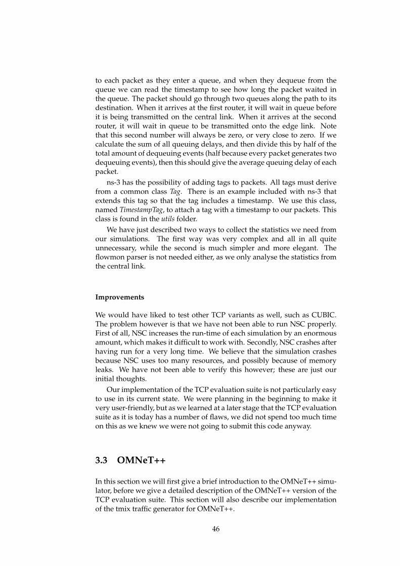
to each packet as they enter a queue, and when they dequeue from thequeue we can read the timestamp to see how long the packet waited inthe queue. The packet should go through two queues along the path to itsdestination. When it arrives at the first router, it will wait in queue beforeit is being transmitted on the central link. When it arrives at the secondrouter, it will wait in queue to be transmitted onto the edge link. Notethat this second number will always be zero, or very close to zero. If wecalculate the sum of all queuing delays, and then divide this by half of thetotal amount of dequeuing events (half because every packet generates twodequeuing events), then this should give the average queuing delay of eachpacket.

ns-3 has the possibility of adding tags to packets. All tags must derivefrom a common class Tag. There is an example included with ns-3 thatextends this tag so that the tag includes a timestamp. We use this class,named TimestampTag, to attach a tag with a timestamp to our packets. Thisclass is found in the utils folder.

We have just described two ways to collect the statistics we need fromour simulations. The first way was very complex and all in all quiteunnecessary, while the second is much simpler and more elegant. Theflowmon parser is not needed either, as we only analyse the statistics fromthe central link.

Improvements

We would have liked to test other TCP variants as well, such as CUBIC.The problem however is that we have not been able to run NSC properly.First of all, NSC increases the run-time of each simulation by an enormousamount, which makes it difficult to work with. Secondly, NSC crashes afterhaving run for a very long time. We believe that the simulation crashesbecause NSC uses too many resources, and possibly because of memoryleaks. We have not been able to verify this however; these are just ourinitial thoughts.

Our implementation of the TCP evaluation suite is not particularly easyto use in its current state. We were planning in the beginning to make itvery user-friendly, but as we learned at a later stage that the TCP evaluationsuite as it is today has a number of flaws, we did not spend too much timeon this as we knew we were not going to submit this code anyway.

3.3 OMNeT++

In this section we will first give a brief introduction to the OMNeT++ simu-lator, before we give a detailed description of the OMNeT++ version of theTCP evaluation suite. This section will also describe our implementationof the tmix traffic generator for OMNeT++.

46

3.3.1 Introduction

This section is a summary of the most vital information from the OMNeT++user manual [10]. OMNeT++ is often quoted as a network simulator[35],but is in fact a generic architecture that can be used in a number ofproblem domains, for instance: network modelling, protocol modelling,modelling of multiprocessors, and validation of hardware architecturesamongst others. OMNeT++ provides infrastructure and tools for writingdifferent kinds of simulations. It also provides a number of utilities to usetogether with the simulation, e.g., classes for random number generation,statistics collection and topology discovery.

OMNeT++ in itself is quite basic and will in most cases be used togetherwith other frameworks. OMNeT++ provides a very basic architecture fordesigning and connecting components. A simulation model is assembledfrom several reusable components, called modules. These modules are thebasic building blocks of any model and can be connected to each othermuch in the same way that one might connect LEGO-blocks. Modulesare connected via gates (the input and output interfaces of a module) andcommunicate with each other by passing messages. These messages maypass through a pre-defined route (as defined by the gate connections), orthey may be sent directly to a destination gate without passing throughconnections. The latter may be useful in simulating wireless connectionsfor instance. A module may also send messages to itself. This is used toschedule events within a module.

The smallest building block in an OMNeT++ simulation is called asimple module. Simple modules may be combined to create compoundmodules. An example of this could be implementing each component ofthe TCP/IP protocol stack as their own module, and combining all thesemodules into a larger compound module, representing a node on thenetwork containing the entire TCP/IP stack. In Figure 3.1, we can see acompound module named StandardNode from the INET framework. Itconsists of a number of modules, some of which are connected, and some ofwhich are not. The entire TCP/IP stack is represented in the figure. At thebottom we have a number of different link-layer protocols, wireless LAN,Ethernet, PPP and optional extensions. These have connections to the gatesof StandardNode, which are represented by the lines going from the link-layer protocols to the bottom. Note that the only way to communicate withthis node is to go through the gates at the bottom and through the link-layerprotocols. All the link-layer protocols are connected to the network layer,which includes the IP protocol. The network layer is connected to threetransport-layer protocols: tcp, udp and sctp. These are again connected toapplication at the top. In addition to the protocols, the StandardNode alsocontains a few other modules, which we will not go into details about here.

Simple modules are written in C++. This is a level of abstraction thatmakes it possible to write very detailed modules (i.e., close to real worldimplementations), while still having all the power of a full object orientedprogramming language. A simulation model in OMNeT++ is referred to

47

Figure 3.1: TCP/IP stack in OMNeT++

48

as a network. A network consists of hierarchical nested modules, where thetop level module is called the system module.

While the module functionality is written in C++, the module structure,and its sections, are described in OMNeT++’s NED language. This is a verysimple scripting language that describes for instance how many gates amodule should have, how each gate is connected to other gates and whichsubmodules a compound module consist of. Each module in OMNeT++may contain several sections that together describe the module, all of themare optional:

• types

• parameters

• gates

• submodules

• connections

The types defined in a NED file are really just local variables, used withinthe NED file. Parameters are variables that belong to a module. They canbe used to specify attributes such as the protocol to be used, the number ofnodes in a simulation, packet length and so on. The NED file also specifiesgates as already mentioned. These are the connection points betweenmodules in a simulation model. When defining a compound module,the submodules will have to be defined as well. Lastly, connectionsbetween gates are also defined using the NED language. When specifyinga connection, we may define simple attributes along with the connection,such as delay and bandwidth, but there are also more complex connectionsincluding loss rate etc.

Configuration and input data for the simulation are in a configurationfile, normally named omnetpp.ini. This file is line oriented and consistsof section headers, or key-value lines. When running an OMNeT++simulation, you get to choose from the different sections defined in theconfiguration file. The most commonly used section is the General section,which is the one used by default. This section will usually contain a baseconfiguration for all your simulations, while the other sections will containthe specifics of each single simulation. In each section there are key-valuelines, where the key is the path of a module parameter, and value is thevalue of the parameter. For instance "Network.server.transactionsPerSecond= 100" will find the Network named Network, then a node of some sortnamed server, and then the transactionsPerSecond parameter of the server.The configuration file accepts wildcard patterns as well, making it easyto configure groups of similar modules. A single asterisk matches zeroor more characters except for dots (which means that it will only matcha single module), while two asterisks match zero or more charactersincluding dots (which means that it may match several modules). Forinstance, ’**.tcpType = "TCPReno"’ will match any network and any node

49

and look for a parameter named tcpType. It will then set this type to"TCPReno" in every module that contains this parameter.

Collecting statistics is an important part of any simulation. OMNeT++provides built-in support for recording simulation results, via output vectorsor output scalars. Output vectors are time series data, recorded from simplemodules or channels. Examples of output vectors may include the round-trip-time (RTT) of each packet between a pair of nodes, the queuing time ofeach packet in a queue or packet drops. Output scalars on the other hand,are summary results. These scalars are computed while the simulationruns, and written out when the simulation ends. These scalars are typicallystatistical summaries of several fields. For instance, output scalars maybe results such as the number of packets dropped at a queue, the averagequeuing time for a flow, the longest RTT ever measured, the average linkutilization and so on.

There are two fundamental ways of recording statistics in OMNeT++.The first is based on the signal mechanism, which was introduced inOMNeT++ 4.1, while the second is based on directly recording statistics inthe C++ code by using the simulation library. The signal mechanism is thepreferred method of handling statistics according to the manual. Signalsare emitted by components. They are identified by signal names. Othermodules may listen to signals, and act whenever a signal of the appropriatetype occurs, or the signals may be used to generate statistics. When a signalis emitted, it can carry a value with it. The value may be a few selectedprimitive types, such as integers, or it may carry an object pointer, such asa pointer to a cPacket.

Statistics are declared in a module’s NED file by the @statistics property.A statistic is based on one or more signals. The statistic may be very simpleby just outputting a simple signal, thus outputting a vector containing allof the signals from the same signal ID. This could for instance be a vectorcontaining all the packets that were dropped. The statistic may be morecomplex as well by generating aggregate statistics , such as the sum of alllost bytes in the simulation.

In the IDE included with OMNeT++, there is an analysis tool thatis very helpful. This tool reads OMNeT++ output files and has thepossibility of combining chosen values into datasets, on which it is possibleto perform certain actions. These actions include computing the averageof all sums, multiplying values, dividing values and so on. In addition tomathematical functions, it is possible to output datasets in (amongst others)comma-separated values (CSV) format, which is useful for further analysis.According to the manual, the IDE’s analysis tool lacks a bit in handlingscalars, and suggests using other tools such as R [12], which is a toolfor statistical computing. The signal mechanism, along with the analysistool found in the IDE makes it relatively easy to work with statistics inOMNeT++.

The basic simulation framework however is not enough for ourpurpose. In addition to the OMNeT++ simulator, we have used the INETframework [5] to add Internet functionality to our simulations. The INETframework contains the most common Internet protocols, such as IPv4,

50

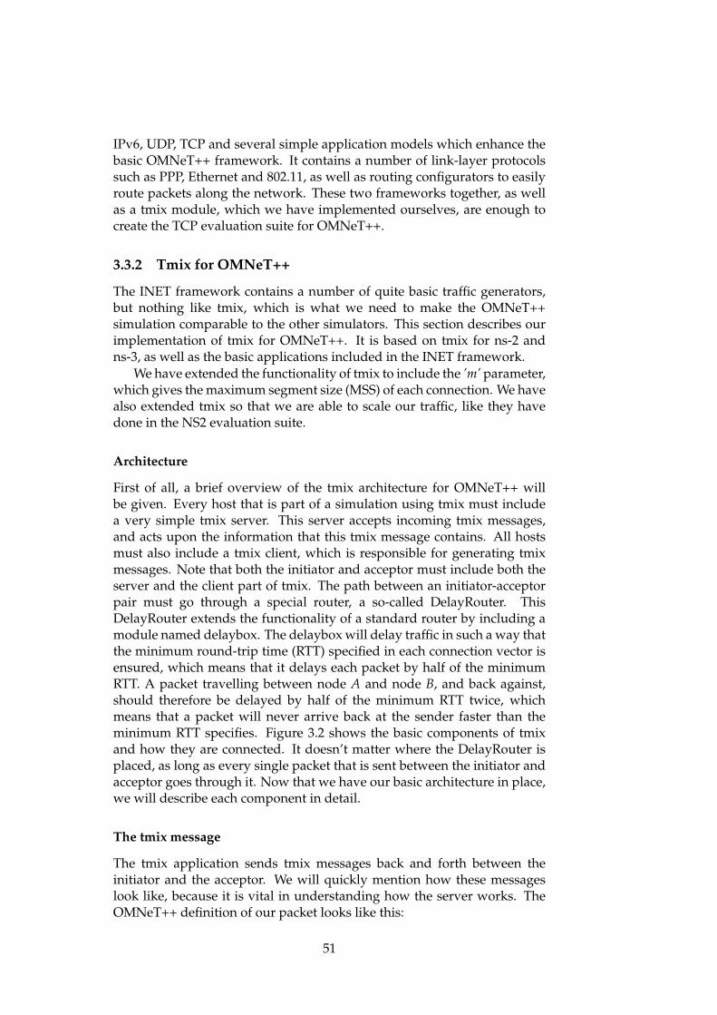
IPv6, UDP, TCP and several simple application models which enhance thebasic OMNeT++ framework. It contains a number of link-layer protocolssuch as PPP, Ethernet and 802.11, as well as routing configurators to easilyroute packets along the network. These two frameworks together, as wellas a tmix module, which we have implemented ourselves, are enough tocreate the TCP evaluation suite for OMNeT++.

3.3.2 Tmix for OMNeT++

The INET framework contains a number of quite basic traffic generators,but nothing like tmix, which is what we need to make the OMNeT++simulation comparable to the other simulators. This section describes ourimplementation of tmix for OMNeT++. It is based on tmix for ns-2 andns-3, as well as the basic applications included in the INET framework.

We have extended the functionality of tmix to include the ’m’ parameter,which gives the maximum segment size (MSS) of each connection. We havealso extended tmix so that we are able to scale our traffic, like they havedone in the NS2 evaluation suite.

Architecture

First of all, a brief overview of the tmix architecture for OMNeT++ willbe given. Every host that is part of a simulation using tmix must includea very simple tmix server. This server accepts incoming tmix messages,and acts upon the information that this tmix message contains. All hostsmust also include a tmix client, which is responsible for generating tmixmessages. Note that both the initiator and acceptor must include both theserver and the client part of tmix. The path between an initiator-acceptorpair must go through a special router, a so-called DelayRouter. ThisDelayRouter extends the functionality of a standard router by including amodule named delaybox. The delaybox will delay traffic in such a way thatthe minimum round-trip time (RTT) specified in each connection vector isensured, which means that it delays each packet by half of the minimumRTT. A packet travelling between node A and node B, and back against,should therefore be delayed by half of the minimum RTT twice, whichmeans that a packet will never arrive back at the sender faster than theminimum RTT specifies. Figure 3.2 shows the basic components of tmixand how they are connected. It doesn’t matter where the DelayRouter isplaced, as long as every single packet that is sent between the initiator andacceptor goes through it. Now that we have our basic architecture in place,we will describe each component in detail.

The tmix message

The tmix application sends tmix messages back and forth between theinitiator and the acceptor. We will quickly mention how these messageslook like, because it is vital in understanding how the server works. TheOMNeT++ definition of our packet looks like this:

51

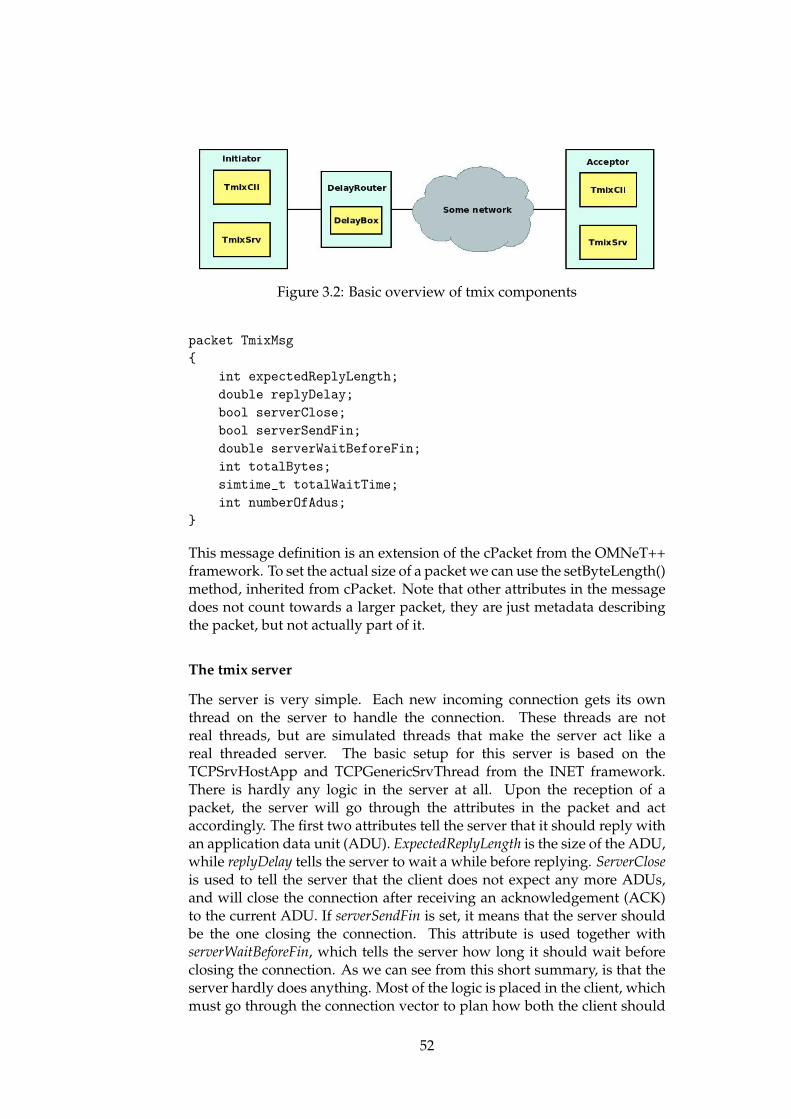
Figure 3.2: Basic overview of tmix components

packet TmixMsg{

int expectedReplyLength;double replyDelay;bool serverClose;bool serverSendFin;double serverWaitBeforeFin;int totalBytes;simtime_t totalWaitTime;int numberOfAdus;

}

This message definition is an extension of the cPacket from the OMNeT++framework. To set the actual size of a packet we can use the setByteLength()method, inherited from cPacket. Note that other attributes in the messagedoes not count towards a larger packet, they are just metadata describingthe packet, but not actually part of it.

The tmix server

The server is very simple. Each new incoming connection gets its ownthread on the server to handle the connection. These threads are notreal threads, but are simulated threads that make the server act like areal threaded server. The basic setup for this server is based on theTCPSrvHostApp and TCPGenericSrvThread from the INET framework.There is hardly any logic in the server at all. Upon the reception of apacket, the server will go through the attributes in the packet and actaccordingly. The first two attributes tell the server that it should reply withan application data unit (ADU). ExpectedReplyLength is the size of the ADU,while replyDelay tells the server to wait a while before replying. ServerCloseis used to tell the server that the client does not expect any more ADUs,and will close the connection after receiving an acknowledgement (ACK)to the current ADU. If serverSendFin is set, it means that the server shouldbe the one closing the connection. This attribute is used together withserverWaitBeforeFin, which tells the server how long it should wait beforeclosing the connection. As we can see from this short summary, is that theserver hardly does anything. Most of the logic is placed in the client, whichmust go through the connection vector to plan how both the client should

52

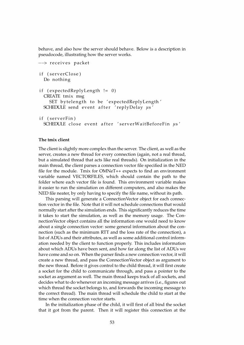
behave, and also how the server should behave. Below is a description inpseudocode, illustrating how the server works.

−−> r e c e i v e s packet

i f ( serverClose )Do nothing

i f ( expectedReplyLength != 0)CREATE tmix msg

SET byte length to be ’ expectedReplyLength ’SCHEDULE send event a f t e r ’ replyDelay µs ’

i f ( serverF in )SCHEDULE c l o s e event a f t e r ’ serverWaitBeforeFin µs ’

The tmix client

The client is slightly more complex than the server. The client, as well as theserver, creates a new thread for every connection (again, not a real thread,but a simulated thread that acts like real threads). On initialization in themain thread, the client parses a connection vector file specified in the NEDfile for the module. Tmix for OMNeT++ expects to find an environmentvariable named VECTORFILES, which should contain the path to thefolder where each vector file is found. This environment variable makesit easier to run the simulation on different computers, and also makes theNED file neater, by only having to specify the file name, without its path.

This parsing will generate a ConnectionVector object for each connec-tion vector in the file. Note that it will not schedule connections that wouldnormally start after the simulation ends. This significantly reduces the timeit takes to start the simulation, as well as the memory usage. The Con-nectionVector object contains all the information one would need to knowabout a single connection vector: some general information about the con-nection (such as the minimum RTT and the loss rate of the connection), alist of ADUs and their attributes, as well as some additional control inform-ation needed by the client to function properly. This includes informationabout which ADUs have been sent, and how far along the list of ADUs wehave come and so on. When the parser finds a new connection vector, it willcreate a new thread, and pass the ConnectionVector object as argument tothe new thread. Before it gives control to the child thread, it will first createa socket for the child to communicate through, and pass a pointer to thesocket as argument as well. The main thread keeps track of all sockets, anddecides what to do whenever an incoming message arrives (i.e., figures outwhich thread the socket belongs to, and forwards the incoming message tothe correct thread). The main thread will schedule the child to start at thetime when the connection vector starts.

In the initialization phase of the child, it will first of all bind the socketthat it got from the parent. Then it will register this connection at the

53

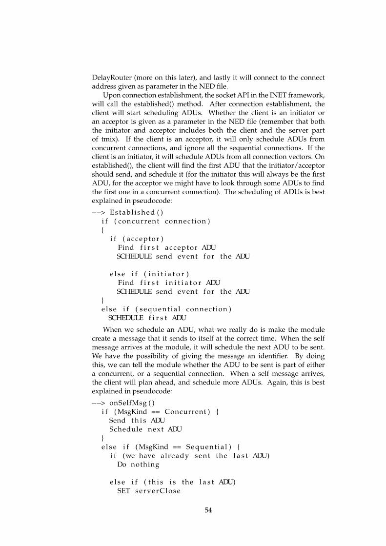
DelayRouter (more on this later), and lastly it will connect to the connectaddress given as parameter in the NED file.

Upon connection establishment, the socket API in the INET framework,will call the established() method. After connection establishment, theclient will start scheduling ADUs. Whether the client is an initiator oran acceptor is given as a parameter in the NED file (remember that boththe initiator and acceptor includes both the client and the server partof tmix). If the client is an acceptor, it will only schedule ADUs fromconcurrent connections, and ignore all the sequential connections. If theclient is an initiator, it will schedule ADUs from all connection vectors. Onestablished(), the client will find the first ADU that the initiator/acceptorshould send, and schedule it (for the initiator this will always be the firstADU, for the acceptor we might have to look through some ADUs to findthe first one in a concurrent connection). The scheduling of ADUs is bestexplained in pseudocode:

−−> Es t ab l i s h ed ( )i f ( concurrent connect ion ){

i f ( acceptor )Find f i r s t acceptor ADUSCHEDULE send event f o r the ADU

e l s e i f ( i n i t i a t o r )Find f i r s t i n i t i a t o r ADUSCHEDULE send event f o r the ADU

}e l s e i f ( s e q u e n t i a l connect ion )

SCHEDULE f i r s t ADU

When we schedule an ADU, what we really do is make the modulecreate a message that it sends to itself at the correct time. When the selfmessage arrives at the module, it will schedule the next ADU to be sent.We have the possibility of giving the message an identifier. By doingthis, we can tell the module whether the ADU to be sent is part of eithera concurrent, or a sequential connection. When a self message arrives,the client will plan ahead, and schedule more ADUs. Again, this is bestexplained in pseudocode:

−−> onSelfMsg ( )i f ( MsgKind == Concurrent ) {

Send t h i s ADUSchedule next ADU

}e l s e i f ( MsgKind == Sequent ia l ) {

i f (we have already sent the l a s t ADU)Do nothing

e l s e i f ( t h i s i s the l a s t ADU)SET serverClose

54

SEND t h i s ADU

e l s e i f (we should send two packets in a row )SEND t h i s ADUSCHEDULE next ADU

e l s e i f ( the next ADU i s the l a s t ADU)SET serverSendFinSET serverWaitBeforeFin to zeroSEND t h i s ADU

e l s e i f ( the two next ADUs are acceptor ADUs)SET serverSendFinSET serverWaitBeforeFinSEND t h i s ADU

e l s eSEND t h i s ADU

}

In the ConnectionVector object we keep a bit of additional information thatis not really part of the connection vector, but is rather used as a part of theclient algorithm. This includes an index to tell how far along the ADUs wehave come. Whenever we send a message, we increase this index as well,so that we know which ADU is the next one to send. When we receive aself message, handling a concurrent connection is very easy, as the client isnot depending on the server it is communicating with. As we do not haveto wait for ADUs from the server, we can just send the current ADU, andschedule the next ADU right away.

Sequential connections are a little more complex (note that onlyinitiators schedule ADUs from sequential connections). The first thing wecheck is whether our index has been increased beyond the number of ADUswe should send. If so, we do not have to do anything, as the last ADU hasalready been sent. If the current ADU happens to have the last index, wecan send the ADU, and tell the server that the current ADU is the last ADUand that we do not expect to get a reply (other than the ACK, but thatdoes not involve the server application, only the TCP module). If there aretwo packets in a row that are both sent from the initiator, we send the firstone, and schedule the next one. When we are getting near the end of aconnection vector, we will have to plan ahead to see how we should closethe connection. If the next ADU is the last ADU, then we know that theserver should close the connection right away, so that is what we tell it todo. The last conditional statement checks whether there are two ADUs ina row, both from the acceptor. This only happens in one special case. Thefirst of these two ADUs is a normal one, while the second ADU is a specialADU where the size if zero. This second ADU means that the server shouldclose the connection, and this ADU also specifies a wait time. This meansthat the server should send the first normal ADU, and then it should waitthe time specified in the second ADU before it closes the connection. So

55

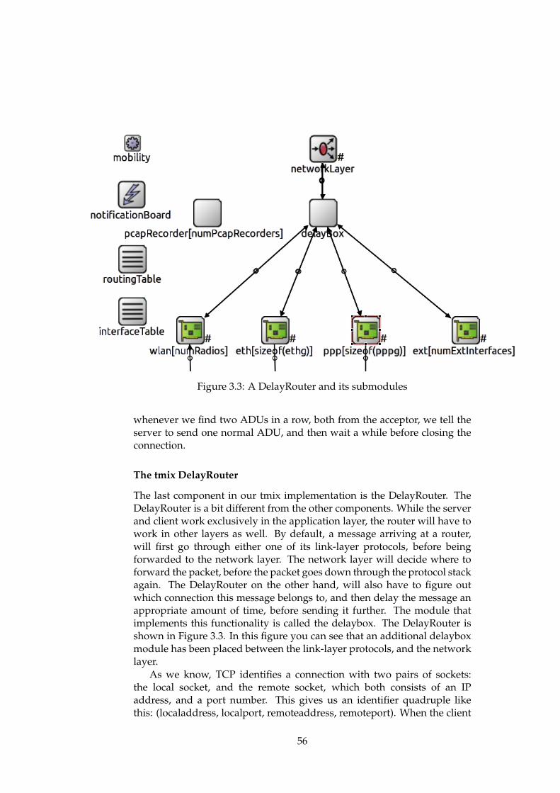
Figure 3.3: A DelayRouter and its submodules

whenever we find two ADUs in a row, both from the acceptor, we tell theserver to send one normal ADU, and then wait a while before closing theconnection.

The tmix DelayRouter

The last component in our tmix implementation is the DelayRouter. TheDelayRouter is a bit different from the other components. While the serverand client work exclusively in the application layer, the router will have towork in other layers as well. By default, a message arriving at a router,will first go through either one of its link-layer protocols, before beingforwarded to the network layer. The network layer will decide where toforward the packet, before the packet goes down through the protocol stackagain. The DelayRouter on the other hand, will also have to figure outwhich connection this message belongs to, and then delay the message anappropriate amount of time, before sending it further. The module thatimplements this functionality is called the delaybox. The DelayRouter isshown in Figure 3.3. In this figure you can see that an additional delayboxmodule has been placed between the link-layer protocols, and the networklayer.

As we know, TCP identifies a connection with two pairs of sockets:the local socket, and the remote socket, which both consists of an IPaddress, and a port number. This gives us an identifier quadruple likethis: (localaddress, localport, remoteaddress, remoteport). When the client

56

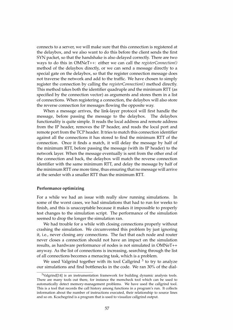
connects to a server, we will make sure that this connection is registered atthe delaybox, and we also want to do this before the client sends the firstSYN packet, so that the handshake is also delayed correctly. There are twoways to do this in OMNeT++: either we can call the registerConnection()method of the delaybox directly, or we can send a message directly to aspecial gate on the delaybox, so that the register connection message doesnot traverse the network and add to the traffic. We have chosen to simplyregister the connection by calling the registerConnection() method directly.This method takes both the identifier quadruple and the minimum RTT (asspecified by the connection vector) as arguments and stores them in a listof connections. When registering a connection, the delaybox will also storethe reverse connection for messages flowing the opposite way.

When a message arrives, the link-layer protocol will first handle themessage, before passing the message to the delaybox. The delayboxfunctionality is quite simple. It reads the local address and remote addressfrom the IP header, removes the IP header, and reads the local port andremote port from the TCP header. It tries to match this connection identifieragainst all the connections it has stored to find the minimum RTT of theconnection. Once it finds a match, it will delay the message by half ofthe minimum RTT, before passing the message (with its IP header) to thenetwork layer. When the message eventually is sent from the other end ofthe connection and back, the delaybox will match the reverse connectionidentifier with the same minimum RTT, and delay the message by half ofthe minimum RTT one more time, thus ensuring that no message will arriveat the sender with a smaller RTT than the minimum RTT.

Performance optimizing

For a while we had an issue with really slow running simulations. Insome of the worst cases, we had simulations that had to run for weeks tofinish, and this is unacceptable because it makes it impossible to properlytest changes to the simulation script. The performance of the simulationseemed to drop the longer the simulation ran.

We had trouble for a while with closing connections properly withoutcrashing the simulation. We circumvented this problem by just ignoringit, i.e., never closing any connections. The fact that each node and routernever closes a connection should not have an impact on the simulationresults, as hardware performance of nodes is not simulated in OMNeT++anyway. As the list of connections is increasing, searching through the listof all connections becomes a menacing task, which is a problem.

We used Valgrind together with its tool Callgrind 3 to try to analyzeour simulations and find bottlenecks in the code. We ran 30% of the dial-

3Valgrind[14] is an instrumentation framework for building dynamic analysis tools.There are many tools out there, for instance the memcheck tool which can be used toautomatically detect memory-management problems. We have used the callgrind tool.This is a tool that records the call history among functions in a program’s run. It collectsinformation about the number of instructions executed, their relationship to source linesand so on. Kcachegrind is a program that is used to visualize callgrind output.

57

Figure 3.4: The callee map before optimization, shown in kCacheGrind

up basic scenario with valgrind to benchmark our simulation. Figure 3.4shows the callee map from callgrind, shown in kCacheGrind. This mapshows all the functions in the simulation, and the size represent how muchof the simulation time has been spent in the function. In the middleof the map we can see a quite noticeable area highlighted. This is theDelayBox’s findDelayForSegment() function, which is the function that looksthrough the connection list to find the minimum RTT of the connection.The rest of the callee map shows a lot of OMNeT++ internal functions.The program spent 12.22% of its time in the findDelayForSegment() function.This number in itself is not a problem, but it confirmed what we expected:that the DelayBox’s lookup function was the main bottleneck. The numberis quite small because we only ran the dial-up basic scenario for 30% ofits time (running the simulation through Valgrind increases its run timesignificantly). This is the scenario with the least amount of traffic. We nowknew that this was the main bottleneck, and we also knew that the list ofconnections was growing without limits, which as a really big problem forthe other scenarios.

The first thought was that we could increase performance by decreasingthe size of the list of connections in the DelayRouter. To do this, we had tofigure out when connections could be safely closed without packets stillbeing in flight. For a while we believed that the algorithm of the client andserver was the problem, that we were actually closing connections at theincorrect time, but this was not the case. The problem was actually just abug in the client. To close a connection we do three things: close the socket,remove the connection from the delaybox, and kill the client thread. Whena client thread closes a socket, it means that the client is done sending ADUsand sends a FIN message. The server replies with its own FIN message.The problem was that when this FIN message arrived back at the mainclient thread, the main thread would still try to pass the FIN message to bethe child thread, although this thread was already removed, thus causing acrash. The easy fix was to just let the main thread handle this FIN messageon its own, rather than passing it to the child thread. We ran the dial-upscenario again for 30% of its time to compare our new simulation. Thecallee map is shown in Figure 3.5. As we can see, the highlighted partof the map is now noticeable smaller. The program now spends 9.36% of

58

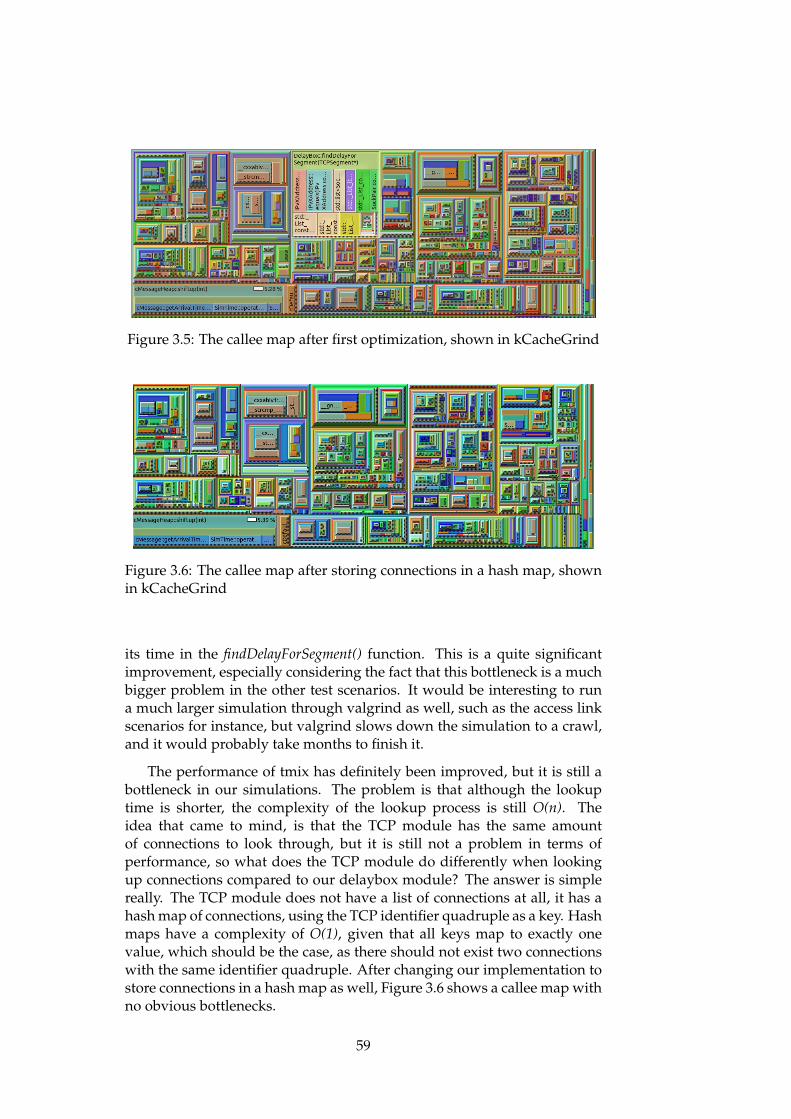
Figure 3.5: The callee map after first optimization, shown in kCacheGrind

Figure 3.6: The callee map after storing connections in a hash map, shownin kCacheGrind

its time in the findDelayForSegment() function. This is a quite significantimprovement, especially considering the fact that this bottleneck is a muchbigger problem in the other test scenarios. It would be interesting to runa much larger simulation through valgrind as well, such as the access linkscenarios for instance, but valgrind slows down the simulation to a crawl,and it would probably take months to finish it.

The performance of tmix has definitely been improved, but it is still abottleneck in our simulations. The problem is that although the lookuptime is shorter, the complexity of the lookup process is still O(n). Theidea that came to mind, is that the TCP module has the same amountof connections to look through, but it is still not a problem in terms ofperformance, so what does the TCP module do differently when lookingup connections compared to our delaybox module? The answer is simplereally. The TCP module does not have a list of connections at all, it has ahash map of connections, using the TCP identifier quadruple as a key. Hashmaps have a complexity of O(1), given that all keys map to exactly onevalue, which should be the case, as there should not exist two connectionswith the same identifier quadruple. After changing our implementation tostore connections in a hash map as well, Figure 3.6 shows a callee map withno obvious bottlenecks.

59

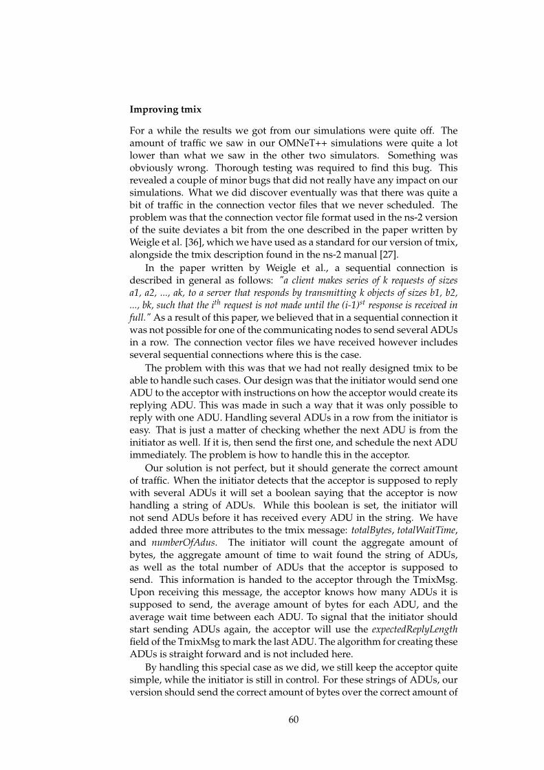
Improving tmix

For a while the results we got from our simulations were quite off. Theamount of traffic we saw in our OMNeT++ simulations were quite a lotlower than what we saw in the other two simulators. Something wasobviously wrong. Thorough testing was required to find this bug. Thisrevealed a couple of minor bugs that did not really have any impact on oursimulations. What we did discover eventually was that there was quite abit of traffic in the connection vector files that we never scheduled. Theproblem was that the connection vector file format used in the ns-2 versionof the suite deviates a bit from the one described in the paper written byWeigle et al. [36], which we have used as a standard for our version of tmix,alongside the tmix description found in the ns-2 manual [27].

In the paper written by Weigle et al., a sequential connection isdescribed in general as follows: "a client makes series of k requests of sizesa1, a2, ..., ak, to a server that responds by transmitting k objects of sizes b1, b2,..., bk, such that the ith request is not made until the (i-1)st response is received infull." As a result of this paper, we believed that in a sequential connection itwas not possible for one of the communicating nodes to send several ADUsin a row. The connection vector files we have received however includesseveral sequential connections where this is the case.

The problem with this was that we had not really designed tmix to beable to handle such cases. Our design was that the initiator would send oneADU to the acceptor with instructions on how the acceptor would create itsreplying ADU. This was made in such a way that it was only possible toreply with one ADU. Handling several ADUs in a row from the initiator iseasy. That is just a matter of checking whether the next ADU is from theinitiator as well. If it is, then send the first one, and schedule the next ADUimmediately. The problem is how to handle this in the acceptor.

Our solution is not perfect, but it should generate the correct amountof traffic. When the initiator detects that the acceptor is supposed to replywith several ADUs it will set a boolean saying that the acceptor is nowhandling a string of ADUs. While this boolean is set, the initiator willnot send ADUs before it has received every ADU in the string. We haveadded three more attributes to the tmix message: totalBytes, totalWaitTime,and numberOfAdus. The initiator will count the aggregate amount ofbytes, the aggregate amount of time to wait found the string of ADUs,as well as the total number of ADUs that the acceptor is supposed tosend. This information is handed to the acceptor through the TmixMsg.Upon receiving this message, the acceptor knows how many ADUs it issupposed to send, the average amount of bytes for each ADU, and theaverage wait time between each ADU. To signal that the initiator shouldstart sending ADUs again, the acceptor will use the expectedReplyLengthfield of the TmixMsg to mark the last ADU. The algorithm for creating theseADUs is straight forward and is not included here.

By handling this special case as we did, we still keep the acceptor quitesimple, while the initiator is still in control. For these strings of ADUs, ourversion should send the correct amount of bytes over the correct amount of

60

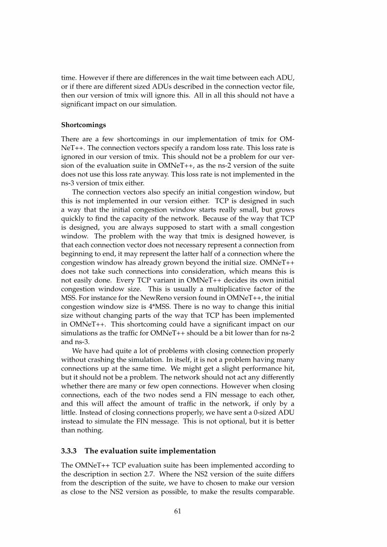
time. However if there are differences in the wait time between each ADU,or if there are different sized ADUs described in the connection vector file,then our version of tmix will ignore this. All in all this should not have asignificant impact on our simulation.

Shortcomings

There are a few shortcomings in our implementation of tmix for OM-NeT++. The connection vectors specify a random loss rate. This loss rate isignored in our version of tmix. This should not be a problem for our ver-sion of the evaluation suite in OMNeT++, as the ns-2 version of the suitedoes not use this loss rate anyway. This loss rate is not implemented in thens-3 version of tmix either.

The connection vectors also specify an initial congestion window, butthis is not implemented in our version either. TCP is designed in sucha way that the initial congestion window starts really small, but growsquickly to find the capacity of the network. Because of the way that TCPis designed, you are always supposed to start with a small congestionwindow. The problem with the way that tmix is designed however, isthat each connection vector does not necessary represent a connection frombeginning to end, it may represent the latter half of a connection where thecongestion window has already grown beyond the initial size. OMNeT++does not take such connections into consideration, which means this isnot easily done. Every TCP variant in OMNeT++ decides its own initialcongestion window size. This is usually a multiplicative factor of theMSS. For instance for the NewReno version found in OMNeT++, the initialcongestion window size is 4*MSS. There is no way to change this initialsize without changing parts of the way that TCP has been implementedin OMNeT++. This shortcoming could have a significant impact on oursimulations as the traffic for OMNeT++ should be a bit lower than for ns-2and ns-3.

We have had quite a lot of problems with closing connection properlywithout crashing the simulation. In itself, it is not a problem having manyconnections up at the same time. We might get a slight performance hit,but it should not be a problem. The network should not act any differentlywhether there are many or few open connections. However when closingconnections, each of the two nodes send a FIN message to each other,and this will affect the amount of traffic in the network, if only by alittle. Instead of closing connections properly, we have sent a 0-sized ADUinstead to simulate the FIN message. This is not optional, but it is betterthan nothing.

3.3.3 The evaluation suite implementation

The OMNeT++ TCP evaluation suite has been implemented according tothe description in section 2.7. Where the NS2 version of the suite differsfrom the description of the suite, we have to chosen to make our versionas close to the NS2 version as possible, to make the results comparable.

61

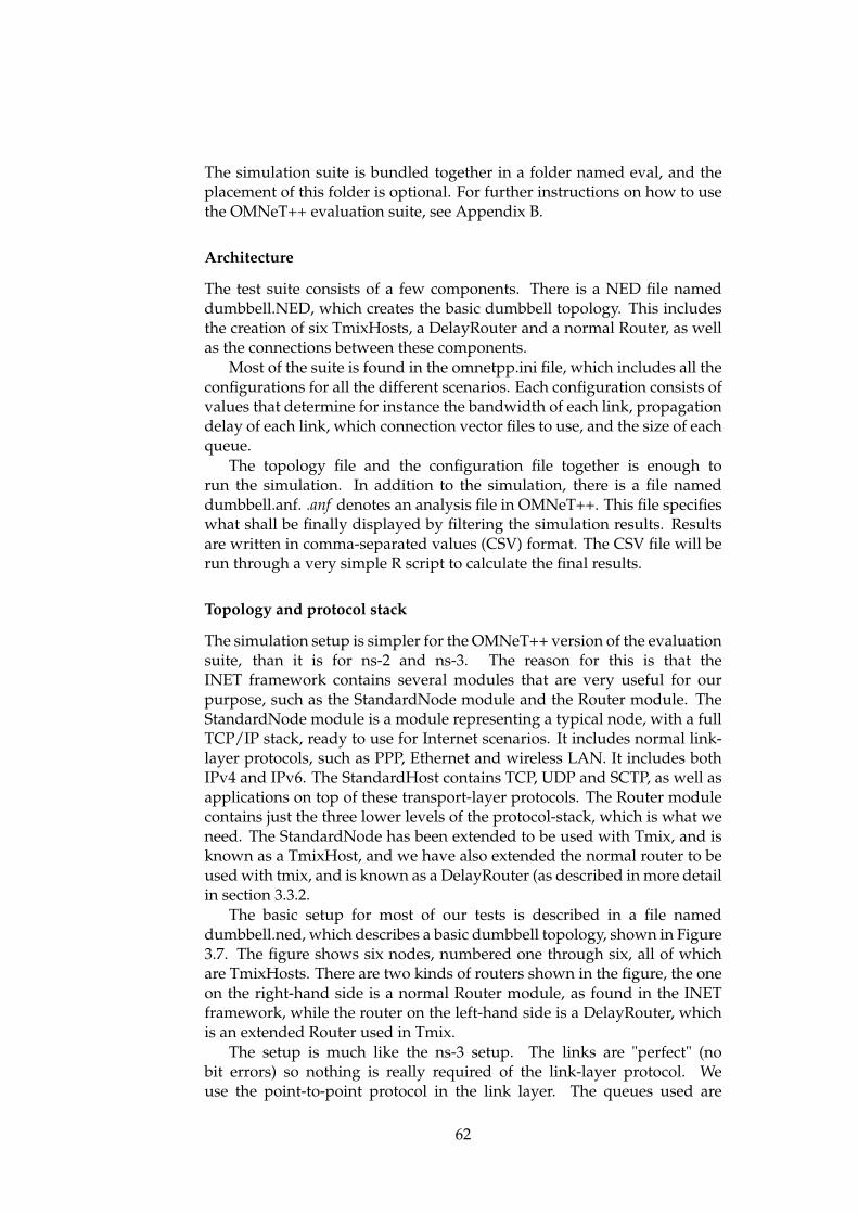
The simulation suite is bundled together in a folder named eval, and theplacement of this folder is optional. For further instructions on how to usethe OMNeT++ evaluation suite, see Appendix B.

Architecture

The test suite consists of a few components. There is a NED file nameddumbbell.NED, which creates the basic dumbbell topology. This includesthe creation of six TmixHosts, a DelayRouter and a normal Router, as wellas the connections between these components.

Most of the suite is found in the omnetpp.ini file, which includes all theconfigurations for all the different scenarios. Each configuration consists ofvalues that determine for instance the bandwidth of each link, propagationdelay of each link, which connection vector files to use, and the size of eachqueue.

The topology file and the configuration file together is enough torun the simulation. In addition to the simulation, there is a file nameddumbbell.anf. .anf denotes an analysis file in OMNeT++. This file specifieswhat shall be finally displayed by filtering the simulation results. Resultsare written in comma-separated values (CSV) format. The CSV file will berun through a very simple R script to calculate the final results.

Topology and protocol stack

The simulation setup is simpler for the OMNeT++ version of the evaluationsuite, than it is for ns-2 and ns-3. The reason for this is that theINET framework contains several modules that are very useful for ourpurpose, such as the StandardNode module and the Router module. TheStandardNode module is a module representing a typical node, with a fullTCP/IP stack, ready to use for Internet scenarios. It includes normal link-layer protocols, such as PPP, Ethernet and wireless LAN. It includes bothIPv4 and IPv6. The StandardHost contains TCP, UDP and SCTP, as well asapplications on top of these transport-layer protocols. The Router modulecontains just the three lower levels of the protocol-stack, which is what weneed. The StandardNode has been extended to be used with Tmix, and isknown as a TmixHost, and we have also extended the normal router to beused with tmix, and is known as a DelayRouter (as described in more detailin section 3.3.2.

The basic setup for most of our tests is described in a file nameddumbbell.ned, which describes a basic dumbbell topology, shown in Figure3.7. The figure shows six nodes, numbered one through six, all of whichare TmixHosts. There are two kinds of routers shown in the figure, the oneon the right-hand side is a normal Router module, as found in the INETframework, while the router on the left-hand side is a DelayRouter, whichis an extended Router used in Tmix.

The setup is much like the ns-3 setup. The links are "perfect" (nobit errors) so nothing is really required of the link-layer protocol. Weuse the point-to-point protocol in the link layer. The queues used are

62

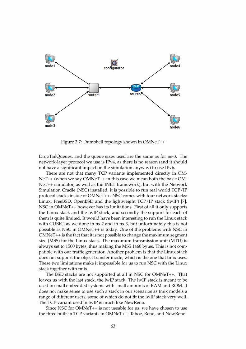
Figure 3.7: Dumbbell topology shown in OMNeT++

DropTailQueues, and the queue sizes used are the same as for ns-3. Thenetwork-layer protocol we use is IPv4, as there is no reason (and it shouldnot have a significant impact on the simulation anyway) to use IPv6.

There are not that many TCP variants implemented directly in OM-NeT++ (when we say OMNeT++ in this case we mean both the basic OM-NeT++ simulator, as well as the INET framework), but with the NetworkSimulation Cradle (NSC) installed, it is possible to run real world TCP/IPprotocol stacks inside of OMNeT++. NSC comes with four network stacks:Linux, FreeBSD, OpenBSD and the lightweight TCP/IP stack (lwIP) [7].NSC in OMNeT++ however has its limitations. First of all it only supportsthe Linux stack and the lwIP stack, and secondly the support for each ofthem is quite limited. It would have been interesting to run the Linux stackwith CUBIC, as we done in ns-2 and in ns-3, but unfortunately this is notpossible as NSC in OMNeT++ is today. One of the problems with NSC inOMNeT++ is the fact that it is not possible to change the maximum segmentsize (MSS) for the Linux stack. The maximum transmission unit (MTU) isalways set to 1500 bytes, thus making the MSS 1460 bytes. This is not com-patible with our traffic generator. Another problem is that the Linux stackdoes not support the object transfer mode, which is the one that tmix uses.These two limitations make it impossible for us to run NSC with the Linuxstack together with tmix.

The BSD stacks are not supported at all in NSC for OMNeT++. Thatleaves us with the last stack, the lwIP stack. The lwIP stack is meant to beused in small embedded systems with small amounts of RAM and ROM. Itdoes not make sense to use such a stack in our scenarios as tmix models arange of different users, some of which do not fit the lwIP stack very well.The TCP variant used in lwIP is much like NewReno.

Since NSC for OMNeT++ is not useable for us, we have chosen to usethe three built-in TCP variants in OMNeT++: Tahoe, Reno, and NewReno.

63

Traffic generation

To generate traffic we have used our own version of tmix implemented forOMNeT++, described in detail in section 3.3.2. Traffic is described througha series of connection vector files, given as input to the simulation throughthe configuration file. There are nine files in total, where one file describesthe traffic between a pair of nodes in the simulation. Each host in thesimulation contains a TmixSrv that the other clients can connect to. Eachnode from the left side connects to every node from the right side and viceversa. All traffic flows through the central link, which means that the nodeson either the left side, or the right, do not communicate among themselves.The setup is the same as in ns-2 and in ns-3.

As mentioned in the section about tmix for OMNeT++, tmix has beenextended so that we have the possibility of scaling traffic. The scales foreach scenario are the same as for the NS2 version of the evaluation suite.

Collecting and presenting statistics

There are a number of statistics to be collected, as described in theevaluation suite. As mentioned, OMNeT++ has a built-in system to handlestatistics, and many of the modules in the INET framework have severalvery useful pre-defined statistics, that we use to collect our statistics. Notethat for every simulation, it is possible to define a warm-up period. In thiswarm-up statistics are not collected. This warm-up period is set accordingto the warm-up periods defined in the evaluation suite.

To get the throughput of the central link, there is a statistic namedrxPkOk:sum(packetBytes) found in the PPP module, which is the sum of allbytes successfully received. We can use this statistic from both the routersto calculate the throughput in each direction. Throughput is here defined asthe number of bits per second traversing the central link, so calculating thethroughput is just a matter of dividing the number of bytes by the numberof seconds that the simulation ran for. This definition of throughput alsomakes it easy to derive the link utilization: throughput divided on the linkcapacity.

To find the drop rate in each direction, there is a statistic nameddropPk:count that is generated by the queue of each router. In addition to thedrop count in each router, there is also a statistic named rxPkOk:count foundin the PPP module of each router, which counts the number of packets thatwere successfully received. These two statistics together makes it possibleto calculate the drop rate.

A histogram is generated for each queue, which shows the queuingtime of each packet. There are also several scalars based on this histogram.These scalars include the aggregate mean queuing delay through the entiresimulation, and the aggregate mean queuing size.

To generate statistics, we have used the analysis tool in the IDE to createa dataset consisting of the values described above. This dataset is writtenas a CSV file, and further run through a basic R script to create the finalstatistics. The R script is very simple: it takes the link capacity as argument,

64

reads the CSV file from OMNeT++, and calculates the final statistics basedon these values.

shortcomings

Our version of tmix skips a few details from the connection vector files.Loss rate is ignored (just like ns-2 and ns-3 does), but also the initialcongestion window size is ignored, which makes our OMNeT++ versionof tmix different to the ones found in ns-2 and ns-3.

As a whole the evaluation suite for OMNeT++ is not very easy to use.Now this is not a big problem really as it will not be released for public useas the TCP evaluation suite suffers from a number of problems. A mainscript to automatically perform every task required to produce the resultsshould have been in place. The main problem with this is that we have usedthe IDE to develop the suite, and to analyse our results using the analysistool that came with the IDE. This analysis tool does not accept commandline commands, which makes it difficult to create such a script. OMNeT++does however include an analysis tool named scavetool that is commandline based. We have not prioritized rewriting the analysis part of the suitehowever, so for now the suite will have to be run in several steps.

65

66

Chapter 4

Simulation results

4.1 Introduction

An important question to answer is: "what are we actually looking for?". TheTCP evaluation suite (described in Section 2.7) defines a number of testscenarios, and a number of metrics that are collected during the course ofthe simulation. There are two general approaches to our analysis:

First of all, there are several studies (which are listed below in theactual analysis) that compare and evaluate existing TCP variants. Thesestudies should give us an indication on how TCP is expected to behaveunder certain conditions. To analyse our results we can use these studies totry and draw some conclusion on the simulated performance of each TCPvariant in the different simulators.

In addition to comparing the results from each simulator with studieson TCP, we will also analyse our results by comparing the results betweenthe simulators to try and see whether they differ in behaviour.

There are several metrics that we can evaluate. Metrics that are veryimportant when evaluating TCP is throughput, delay, and drop rate.There will always be a tradeoff between the three. Sending packets moreaggressively will lead to a higher throughput, but also to a higher delay aswell as a higher drop rate.

In this case we define throughput to be the amount of raw datatransferred over the network per time unit. This also includes all controlpackets, such as ACKs being sent back and forth.

Delay measures the amount of delay a packet suffers when travellingthrough a network. The amount of delay for a single packet increases inseveral steps along the path. It takes an amount of time to push a packetonto a link (based on the link’s bandwidth). It takes a while for the packetto propagate each link, based on the medium used and the length the link.Whenever the packet reaches a router it might have to wait in queue if thenetwork is congested etc. Round-trip time (RTT) is the cumulative delayfor a packet being sent from the sender to the receiver, and back again.While RTT definitely gives an indication on how the network performs,queuing delay (which is the amount of time each packet waits in queue)ignores the network topology and user think times entirely, thus giving a

67

better indication of the congestion level of the network.Drop rate is the number of packets dropped compared to the number

of packets that were successfully delivered. Whether a packet drop occursbecause of congestion (which causes a queue to drop the packet), becauseof bit-errors on the link (which may cause the link-layer protocol to dropthe packet), or because of any other problem that might cause the packetto be lost, does not make a difference to TCP. In our simulations, the onlytype of drop we should see is the one caused by congestion as other details(such as link-layer errors) are abstracted away.

4.2 The expected results

First of all we expect the different TCP variants to behave relative to eachother as seen in other research. In this section we will go through a fewresearch papers that compare the performance of TCP variants to see whatis expected.

Floyd and Fall [19] explore the benefits of adding selective acknow-ledgements (SACK) to TCP. They have a simple simulation setup wherethey send 20 packets and increment the loss rate for every run to see howeach variant reacts to an increased amount of loss. On the first run, onepacket is lost, on the second run, two packets are lost etc. This is done fourtimes. The experiment is run on the original ns simulator. Reno gives op-timal performance when a single packet is dropped. In the presence of asingle drop, Reno fast retransmits the packet before going into fast recov-ery. The problem is that whenever several drops occur in rapid succession,Reno lowers ssthresh several times, which lowers the throughput severely.In the scenarios with three or four lost packets, Reno will have to wait for aretransmit timer to recover. NewReno and Reno with SACK enabled lookquite alike each other. However, the NewReno sender is at most able toretransmit one packet every round-trip time (RTT). They also show thatwhen there are several lost packets from the same window, Tahoe signi-ficantly outperforms Reno, and barely outperforms NewReno. Both Renoand NewReno outperform Tahoe when there are few lost packets from thesame window. They compare the results to a Reno trace taken from ac-tual Internet traffic measurements. They conclude that the trace exhibitsbehaviour that is similar to the one seen in simulation.

Bateman et al. [18] compares the performance of several high speedTCP variants in ns-2 and in a real-world test bed using Linux. Althoughwe do not evaluate high speed TCP variants (such as BIC and CUBIC) inthis thesis because of lack of support, it is interesting to see whether ns-2results are comparable to the real world. They have a simple setup with lowcomplexity (a dumbbell topology) that is meant to highlight the behaviourof the TCP variants, rather than being realistic. They report that the ns-2 simulations in general behave very much like the test-bed does. Theybelieve that ns-2 simulations can be used to report behaviour that reflectsuse of TCP variants in operational use. They use the same code in boththe test-bed and in ns-2, and encourage more possibilities for inclusion of

68

real code in ns-2. Although they conclude that the ns-2 results and testbedresults to be equivalent, they also say that as complexity increases (morecomplex testbed, additional factors such as CPU scheduling hardwarevariations etc.) we may see more variation in the results. All in all theyconclude that ns-2 is a valuable tool to investigate protocols, although thereis always a small uncertainty to whether the results are actually realistic.

Jansen and McGregor [24] present their validation of the NetworkSimulation Cradle (NSC) for ns-2. They compare the results from atestbed network to a simulation using NSC. Both the simulation and thetestbed run the same protocol stack (which is the point of NSC after all).They conclude that the accuracy in results are very good, and that it isworthwhile to use real world based TCP stacks.

We have a good idea on how TCP should behave, but how do we expectthe network simulators to compare to each other? The TCP variants areclearly defined in RFCs, so in theory (given that all the optional options areconfigured identically across the network simulators) they should performvery similar to each other given that the network and traffic generator areequal in all three simulators. We do not expect the results to be exactly thesame across the simulators - that is unrealistic - but we do expect them togive similar results as we model exactly the same scenario in all three.

4.3 ns-2 results

The results from the ns-2 basic scenarios are summarized in Table 4.1 andTable 4.2. Each scenario was run for four TCP variants: Tahoe, Reno,NewReno, and Cubic. For each TCP variant, each scenario was run threetimes with three levels of congestion: no congestion, mild congestion,and moderate congestion. For each run, the throughput, total number ofpackets, total number of dropped packets, average queuing delay, averagequeue size, and loss rate was collected and are presented in the tables.There are five basic scenarios run (the wireless basic scenario is not runas they are not implemented in ns-3 and OMNeT++): Access Link (AL),Data Center (DC), Geostationary Satellite (GS), Trans-Oceanic link (TO),and Dial-Up (DU). The level of traffic is much higher in the reversedirection (from right to left), than it is in the normal direction (left to right),except for in the geostationary satellite connection where the central link isasymmetric. As the reverse direction has the highest amount of traffic, thisis also the direction we will focus on.

CUBIC is a TCP variant that is designed to utilize network resourcesby quickly finding the maximum network capacity. This means that inmost cases, CUBIC should have a very good throughput, although at theexpense of having a higher drop rate. This is seen very clearly in every ns-2 test. CUBIC shows the highest throughput in both directions in almostevery single scenario. CUBIC is very aggressive (at least compared to theother three variants), this is seen very clearly as well, as CUBIC has thehighest drop rate in most scenarios, and especially in the reverse direction.Not surprisingly, on the other end of the scale, we see that Tahoe has the

69

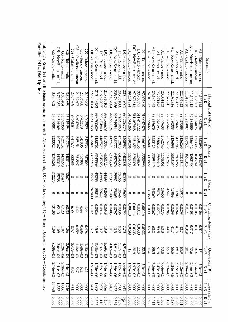
ScenarioT

hroughput(Mbps)

PacketsD

ropsQ

ueueingdelay

(ms)

Queue

size(B)

Lossrate

(%)

L->RR

->LL->R

R->L

L->RR

->LL->R

R->L

L->RR

->LL->R

R->L

AL

-Tahoe-uncon.

11.13599551.855756

12520901844237

00

0.01060.311

172.1e+03

0.0000.000

AL

-Reno

-uncon.11.135803

51.9148251253393

18457410

00.0105

0.31716.6

2.14e+030.000

0.000A

L-N

ewR

eno-uncon.

11.14494852.164500

12564121852138

00

0.01080.317

17.62.16e+03

0.0000.000

AL

-Cubic

-uncon.11.318910

52.2150071257521

18513460

00.0121

0.34920.1

2.38e+030.000

0.000A

L-Tahoe

-mild.

22.05492399.029588

24362663504344

015913

0.025940.7

85.95.12e+05

0.0000.454

AL

-Reno

-mild.

22.06943799.269682

24372033509288

013202

0.026441.5

88.35.22e+05

0.0000.376

AL

-New

Reno

-mild.

22.08263699.080388

24360963503487

017056

0.025941.7

85.55.24e+05

0.0000.487

AL

-Cubic

-mild.

22.67784199.866564

25154193562617

042441

0.028549.4

95.36.23e+05

0.0001.191

AL

-Tahoe-m

od.23.081433

99.9996392562748

35983610

596500.0275

60.893.8

7.64e+050.000

1.658A

L-R

eno-m

od.23.271498

99.9983932556634

35886100

507810.0273

59.591.9

7.47e+050.000

1.415A

L-N

ewR

eno-m

od.23.185062

99.9996702553123

35894450

542650.0267

60.288.3

7.56e+050.000

1.512A

L-C

ubic-m

od.24.019087

99.9996652694802

36698220

1319690.030

65.8104

8.25e+050.000

3.596D

C-Tahoe

-uncon.97.652810

518.0474732166193

33209960

00.00116

0.032222.3

2.1e+030.000

0.000D

C-R

eno-uncon.

99.750395511.491722

21601383294437

00

0.00120.0300

22.91.95e+03

0.0000.000

DC

-New

Reno

-uncon.97.874643

511.4674482151859

32900910

00.00114

0.030320.9

1.97e+030.000

0.000D

C-C

ubic-uncon.

99.461384516.709266

21402063275735

00

0.001100.0298

181.97e+03

0.0000.000

DC

-Tahoe-m

ild.205.449661

993.3367754308987

640050140556

196350.0793

7.734.91e+03

9.64e+050.941

0.307D

C-R

eno-m

ild.205.061808

994.7910684312873

641458539166

185460.0836

8.585.17e+03

1.07e+060.908

0.289D

C-N

ewR

eno-m

ild.203.764636

998.7495444332772

645787639982

238050.0797

10.34.91e+03

1.29e+060.923

0.369D

C-C

ubic-m

ild.212.487884

999.9711244427422

650458917732

1214870.0905

14.14.82e+03

1.77e+060.401

1.868D

C-Tahoe

-mod.

215.310107998.566678

45133546580725

4449392589

0.084913.9

5.69e+031.74e+06

0.9861.407

DC

-Reno

-mod.

216.622035998.674840

44875296545928

4388372642

0.081413.7

5.32e+031.72e+06

0.9781.110

DC

-New

Reno

-mod.

215.408483998.700629

44887026545369

4523388818

0.082613.9

5.48e+031.75e+06

1.0081.357

DC

-Cubic

-mod.

227.701084999.981958

46558926627218

19577262490

0.10215.2

5.54e+031.91e+06

0.4203.961

GS

-Tahoe-uncon.

2.1369088.703579

547936757009

00

4.440.496

1.48e+03621

0.0000.000

GS

-Reno

-uncon.2.136908

8.703579547936

7570090

04.44

0.4961.48e+03

6210.000

0.000G

S-N

ewR

eno-uncon.

2.1326078.604784

545151753597

00

4.420.459

1.48e+03567

0.0000.000

GS

-Cubic

-uncon.2.374769

9.689081641577

8835860

06.55

0.572.47e+03

8020.000

0.000G

S-Tahoe

-mild.

3.80186916.329494

10173941408142

126740

60.301.06

2.96e+042.4e+03

1.2460.000

GS

-Reno

-mild.

3.81848416.292358

10271321430278

185490

67.201.07

3.28e+042.38e+03

1.8060.000

GS

-New

Reno

-mild.

3.79928216.319469

10273671430019

157380

62.101.09

3.04e+042.41e+03

1.5320.000

GS

-Cubic

-mild.

3.98875217.870001

12333211595291

1722700

131.001.09

6.58e+042.74e+03

13.9680.000

Table4.1:R

esultsfrom

thebasic

scenariosfor

ns-2.AL

=A

ccessLink,D

C=

Data

Center,TO

=Trans-O

ceaniclink,G

S=

Geostationary

Satellite,DU

=D

ial-Up

link

70

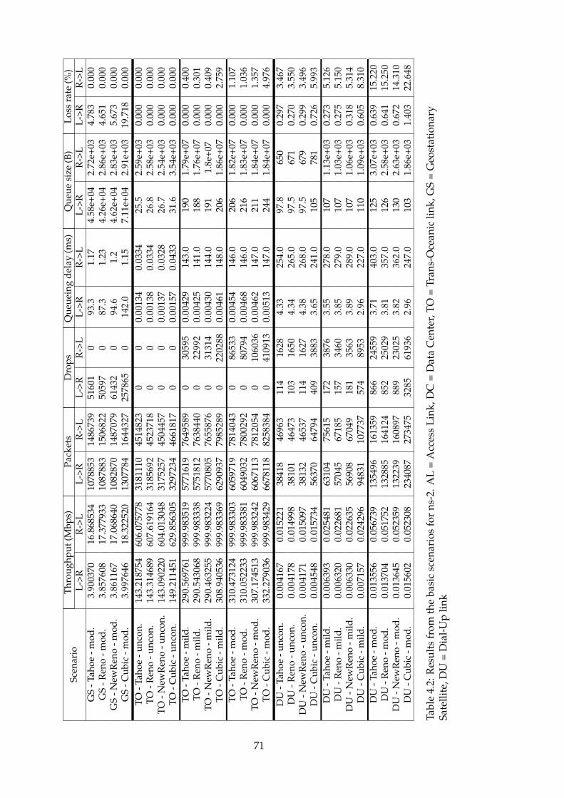
Scen

ario

Thro

ughp

ut(M

bps)

Pack

ets

Dro

psQ

ueue

ing

dela

y(m

s)Q

ueue

size

(B)

Loss

rate

(%)

L->R

R->

LL-

>RR

->L

L->R

R->

LL-

>RR

->L

L->R

R->

LL-

>RR

->L

GS

-Tah

oe-m

od.

3.90

0370

16.8

6853

410

7885

314

8673

951

601

093

.31.

174.

58e+

042.

72e+

034.

783

0.00

0G

S-R

eno

-mod

.3.

8576

0817

.377

933

1087

883

1506

822

5059

70

87.3

1.23

4.26

e+04

2.86

e+03

4.65

10.

000

GS

-New

Ren

o-m

od.

3.86

1167

17.0

6864

010

8287

014

8707

961

432

094

.61.

24.

62e+

042.

83e+

035.

673

0.00

0G

S-C

ubic

-mod

.3.

9976

4618

.322

520

1307

784

1644

327

2578

650

142.

01.

157.

11e+

042.

91e+

0319

.718

0.00

0TO

-Tah

oe-u

ncon

.14

3.21

8754

606.

0757

7831

8111

045

1482

30

00.

0013

40.

0334

25.5

2.59

e+03

0.00

00.

000

TO-R

eno

-unc

on.

143.

3146

8960

7.61

9164

3185

692

4523

718

00

0.00

138

0.03

3426

.82.

58e+

030.

000

0.00

0TO

-New

Ren

o-u

ncon

.14

3.09

0220

604.

0130

4831

7525

745

0445

70

00.

0013

70.

0328

26.7

2.54

e+03

0.00

00.

000

TO-C

ubic

-unc

on.

149.

2114

5162

9.85

6305

3297

234

4661

817

00

0.00

157

0.04

3331

.63.

54e+

030.

000

0.00

0TO

-Tah

oe-m

ild.

290.

5697

6199

9.98

3519

5771

619

7649

589

030

595

0.00

429

143.

019

01.

79e+

070.

000

0.40

0TO

-Ren

o-m

ild.

290.

5430

6899

9.98

3338

5751

812

7638

440

022

992

0.00

425

141.

018

81.

76e+

070.

000

0.30

1TO

-New

Ren

o-m

ild.

290.

4632

5599

9.98

3224

5770

805

7655

876

031

314

0.00

430

144.

019

11.

8e+0

70.

000

0.40

9TO

-Cub

ic-m

ild.

308.

9405

3699

9.98

3369

6290

937

7985

289

022

0288

0.00

461

148.

020

61.

86e+

070.

000

2.75

9TO

-Tah

oe-m

od.

310.

4731

2499

9.98

3303

6059

719

7814

043

086

533

0.00

454

146.

020

61.

82e+

070.

000

1.10

7TO

-Ren

o-m

od.

310.

0522

3399

9.98

3381

6049

032

7800

292

080

794

0.00

468

146.

021

61.

83e+

070.

000

1.03

6TO

-New

Ren

o-m

od.

307.

1745

1399

9.98

3242

6067

113

7812

054

010

6036

0.00

462

147.

021

11.

84e+

070.

000

1.35

7TO

-Cub

ic-m

od.

332.

2790

3699

9.98

3429

6678

118

8258

384

041

0913

0.00

513

147.

024

41.

84e+

070.

000

4.97

6D

U-T

ahoe

-unc

on.

0.00

4167

0.01

5221

3841

846

963

114

1628

4.33

254.

097

.865

00.

297

3.46

7D

U-R

eno

-unc

on.

0.00

4178

0.01

4998

3810

146

473

103

1650

4.34

265.

097

.567

10.

270

3.55

0D

U-N

ewR

eno

-unc

on.

0.00

4171

0.01

5097

3813

246

537

114

1627

4.38

268.

097

.567

90.

299

3.49

6D

U-C

ubic

-unc

on.

0.00

4548

0.01

5734

5637

064

794

409

3883

3.65

241.

010

578

10.

726

5.99

3D

U-T

ahoe

-mild

.0.

0063

930.

0254

8163

104

7561

517

238

763.

5527

8.0

107

1.13

e+03

0.27

35.

126

DU

-Ren

o-m

ild.

0.00

6320

0.02

2681

5704

567

185

157

3460

3.85

279.

010

71.

03e+

030.

275

5.15

0D

U-N

ewR

eno

-mild

.0.

0063

300.

0226

3556

908

6704

918

135

633.

8928

9.0

107

1.06

e+03

0.31

85.

314

DU

-Cub

ic-m

ild.

0.00

7157

0.02

4296

9483

110

7737

574

8953

2.96

227.

011

01.

09e+

030.

605

8.31

0D

U-T

ahoe

-mod

.0.

0135

560.

0567

3913

5496

1613

5986

624

559

3.71

403.

012

53.

07e+

030.

639

15.2

20D

U-R

eno

-mod

.0.

0137

040.

0517

5213

2885

1641

2485

225

029

3.81

357.

012

62.

58e+

030.

641

15.2

50D

U-N

ewR

eno

-mod

.0.

0136

450.

0523

5913

2239

1608

9788

923

025

3.82

362.

013

02.

63e+

030.

672

14.3

10D

U-C

ubic

-mod

.0.

0156

020.

0523

0823

4087

2734

7532

8561

936

2.96

247.

010

31.

86e+

031.

403

22.6

48

Tabl

e4.

2:R

esul

tsfr

omth

eba

sic

scen

ario

sfo

rns

-2.A

L=

Acc

ess

Link

,DC

=D

ata

Cen

ter,

TO=

Tran

s-O

cean

iclin

k,G

S=

Geo

stat

iona

rySa

telli

te,D

U=

Dia

l-U

plin

k

71

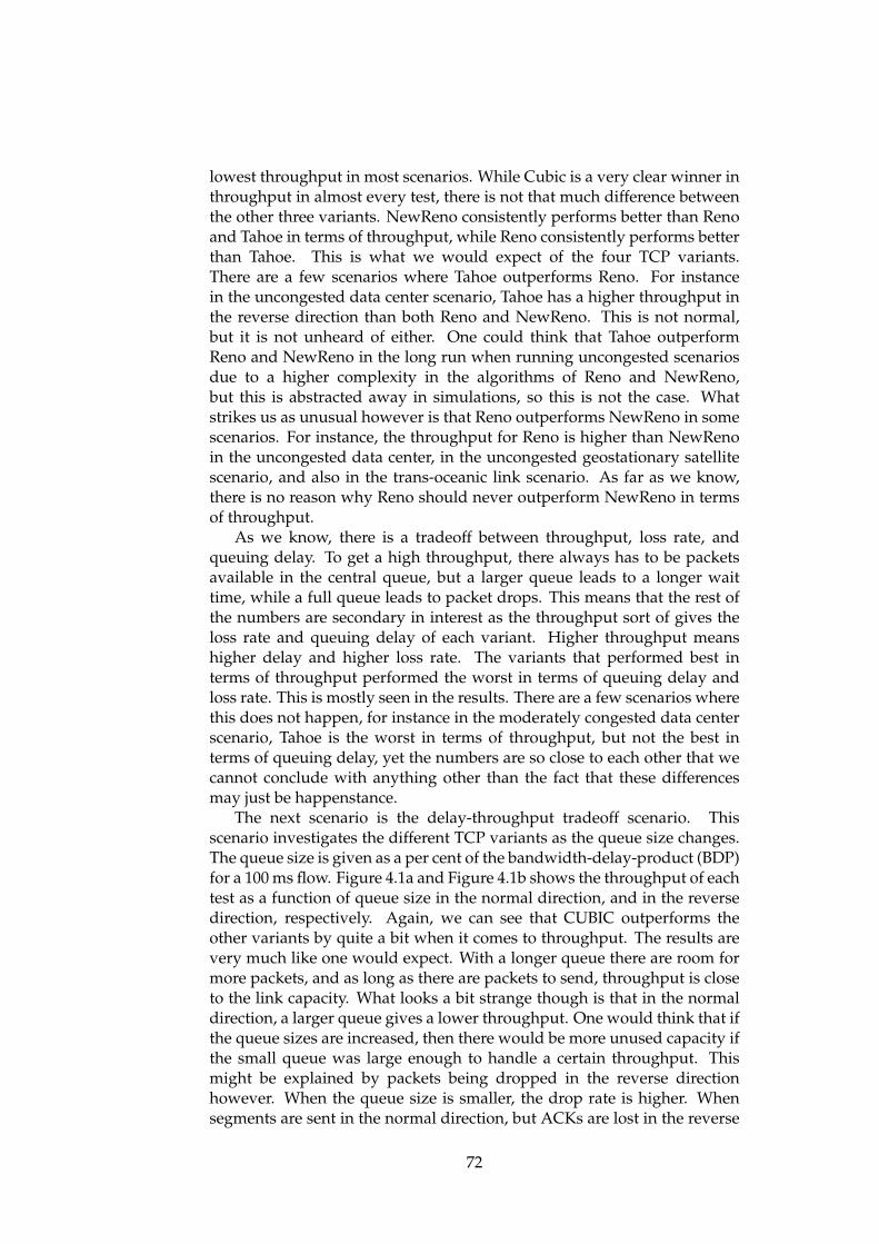
lowest throughput in most scenarios. While Cubic is a very clear winner inthroughput in almost every test, there is not that much difference betweenthe other three variants. NewReno consistently performs better than Renoand Tahoe in terms of throughput, while Reno consistently performs betterthan Tahoe. This is what we would expect of the four TCP variants.There are a few scenarios where Tahoe outperforms Reno. For instancein the uncongested data center scenario, Tahoe has a higher throughput inthe reverse direction than both Reno and NewReno. This is not normal,but it is not unheard of either. One could think that Tahoe outperformReno and NewReno in the long run when running uncongested scenariosdue to a higher complexity in the algorithms of Reno and NewReno,but this is abstracted away in simulations, so this is not the case. Whatstrikes us as unusual however is that Reno outperforms NewReno in somescenarios. For instance, the throughput for Reno is higher than NewRenoin the uncongested data center, in the uncongested geostationary satellitescenario, and also in the trans-oceanic link scenario. As far as we know,there is no reason why Reno should never outperform NewReno in termsof throughput.

As we know, there is a tradeoff between throughput, loss rate, andqueuing delay. To get a high throughput, there always has to be packetsavailable in the central queue, but a larger queue leads to a longer waittime, while a full queue leads to packet drops. This means that the rest ofthe numbers are secondary in interest as the throughput sort of gives theloss rate and queuing delay of each variant. Higher throughput meanshigher delay and higher loss rate. The variants that performed best interms of throughput performed the worst in terms of queuing delay andloss rate. This is mostly seen in the results. There are a few scenarios wherethis does not happen, for instance in the moderately congested data centerscenario, Tahoe is the worst in terms of throughput, but not the best interms of queuing delay, yet the numbers are so close to each other that wecannot conclude with anything other than the fact that these differencesmay just be happenstance.

The next scenario is the delay-throughput tradeoff scenario. Thisscenario investigates the different TCP variants as the queue size changes.The queue size is given as a per cent of the bandwidth-delay-product (BDP)for a 100 ms flow. Figure 4.1a and Figure 4.1b shows the throughput of eachtest as a function of queue size in the normal direction, and in the reversedirection, respectively. Again, we can see that CUBIC outperforms theother variants by quite a bit when it comes to throughput. The results arevery much like one would expect. With a longer queue there are room formore packets, and as long as there are packets to send, throughput is closeto the link capacity. What looks a bit strange though is that in the normaldirection, a larger queue gives a lower throughput. One would think that ifthe queue sizes are increased, then there would be more unused capacity ifthe small queue was large enough to handle a certain throughput. Thismight be explained by packets being dropped in the reverse directionhowever. When the queue size is smaller, the drop rate is higher. Whensegments are sent in the normal direction, but ACKs are lost in the reverse

72

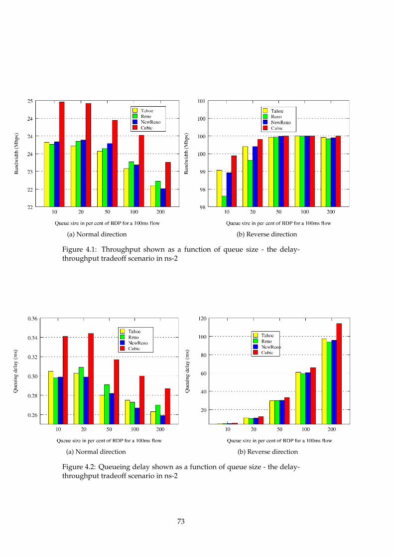
(a) Normal direction (b) Reverse direction

Figure 4.1: Throughput shown as a function of queue size - the delay-throughput tradeoff scenario in ns-2

(a) Normal direction (b) Reverse direction

Figure 4.2: Queueing delay shown as a function of queue size - the delay-throughput tradeoff scenario in ns-2

73

Figure 4.3: Drop rate shown as a function of queue size - the delay-throughput tradeoff scenario in ns-2

direction, this may cause the sender to retransmit segments. This adds tothe average throughput of the link in the normal direction. Because of thiswe actually see a lower throughout in the tests with the largest queues asthere are fewer retransmissions.

As mentioned above, Tahoe is better at handling bursts of packet lossthan Reno and NewReno without SACK. When the queue size is reallysmall, the chance of this happening is much greater; therefore Tahoeoutperforms Reno and NewReno in these cases.

Figure 4.2a and Figure 4.2b show the queuing delay for each test as afunction of queue size in the normal direction, and in the reverse direction,respectively. Again, we can see the throughput-delay tradeoff clearly bycomparing these two graphs to the throughput graphs. A longer queuegives the possibility for longer queuing delay, this is obvious. We can alsosee that the delay of CUBIC is always longer than the delay for the othervariants. This is because of the aggressive nature of CUBIC, always fillingup the queues more than the other variants do. In the normal directionwe see a lower queuing delay for the larger queues. This is explained by ahigher congestion in the reverse direction, as explained above.

Figure 4.3 shows the drop rate of each test as a function of queue size inthe reverse direction. The normal direction is left out because the drop rateis always close to or exactly zero, which is not very interesting. The droprate is much the other way around. A large queue stores more packets fora longer amount of time (as seen in the previous two graphs) instead ofdropping packets. Again, CUBIC, and its aggressive increase in congestionwindow, has a far higher drop rate than any of the other variants. The otherthree variants are more or less equal in terms of drop rate.

The conclusion is that a larger queue gives a better throughput as therealways are packets available to send. A large queue also gives a smallerloss rate as the queue can handle more packets at the same time. However,

74

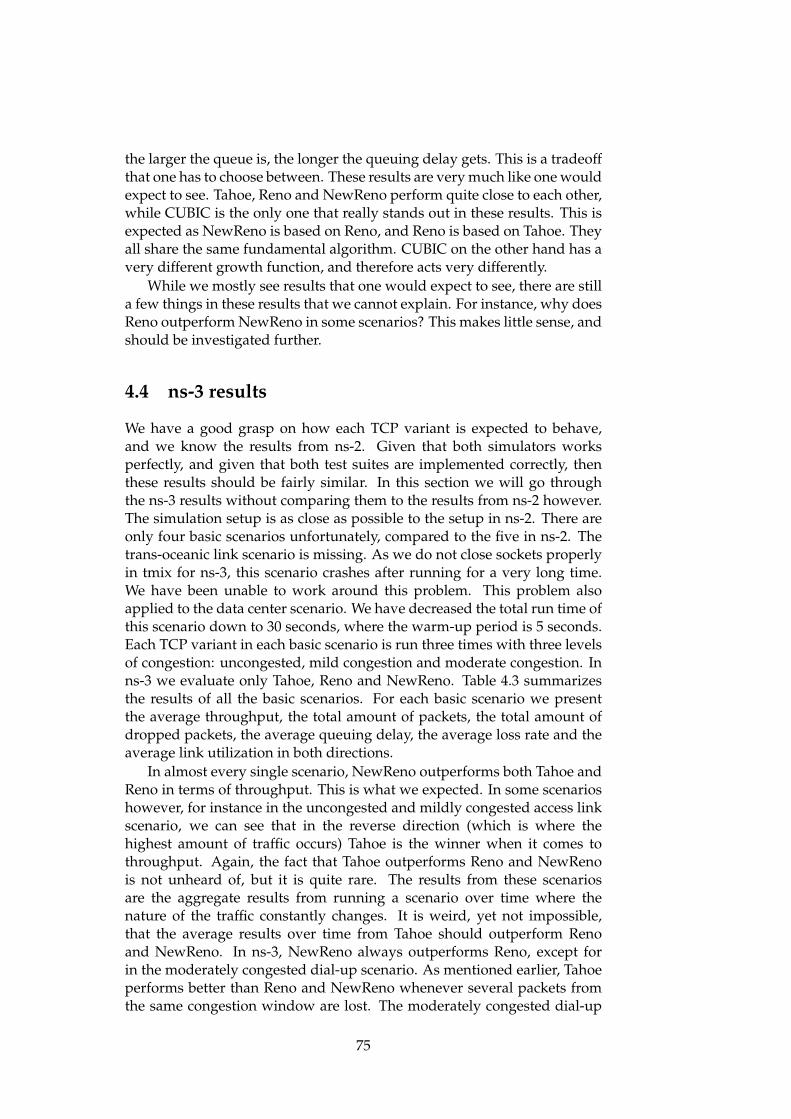
the larger the queue is, the longer the queuing delay gets. This is a tradeoffthat one has to choose between. These results are very much like one wouldexpect to see. Tahoe, Reno and NewReno perform quite close to each other,while CUBIC is the only one that really stands out in these results. This isexpected as NewReno is based on Reno, and Reno is based on Tahoe. Theyall share the same fundamental algorithm. CUBIC on the other hand has avery different growth function, and therefore acts very differently.

While we mostly see results that one would expect to see, there are stilla few things in these results that we cannot explain. For instance, why doesReno outperform NewReno in some scenarios? This makes little sense, andshould be investigated further.

4.4 ns-3 results

We have a good grasp on how each TCP variant is expected to behave,and we know the results from ns-2. Given that both simulators worksperfectly, and given that both test suites are implemented correctly, thenthese results should be fairly similar. In this section we will go throughthe ns-3 results without comparing them to the results from ns-2 however.The simulation setup is as close as possible to the setup in ns-2. There areonly four basic scenarios unfortunately, compared to the five in ns-2. Thetrans-oceanic link scenario is missing. As we do not close sockets properlyin tmix for ns-3, this scenario crashes after running for a very long time.We have been unable to work around this problem. This problem alsoapplied to the data center scenario. We have decreased the total run time ofthis scenario down to 30 seconds, where the warm-up period is 5 seconds.Each TCP variant in each basic scenario is run three times with three levelsof congestion: uncongested, mild congestion and moderate congestion. Inns-3 we evaluate only Tahoe, Reno and NewReno. Table 4.3 summarizesthe results of all the basic scenarios. For each basic scenario we presentthe average throughput, the total amount of packets, the total amount ofdropped packets, the average queuing delay, the average loss rate and theaverage link utilization in both directions.

In almost every single scenario, NewReno outperforms both Tahoe andReno in terms of throughput. This is what we expected. In some scenarioshowever, for instance in the uncongested and mildly congested access linkscenario, we can see that in the reverse direction (which is where thehighest amount of traffic occurs) Tahoe is the winner when it comes tothroughput. Again, the fact that Tahoe outperforms Reno and NewRenois not unheard of, but it is quite rare. The results from these scenariosare the aggregate results from running a scenario over time where thenature of the traffic constantly changes. It is weird, yet not impossible,that the average results over time from Tahoe should outperform Renoand NewReno. In ns-3, NewReno always outperforms Reno, except forin the moderately congested dial-up scenario. As mentioned earlier, Tahoeperforms better than Reno and NewReno whenever several packets fromthe same congestion window are lost. The moderately congested dial-up

75

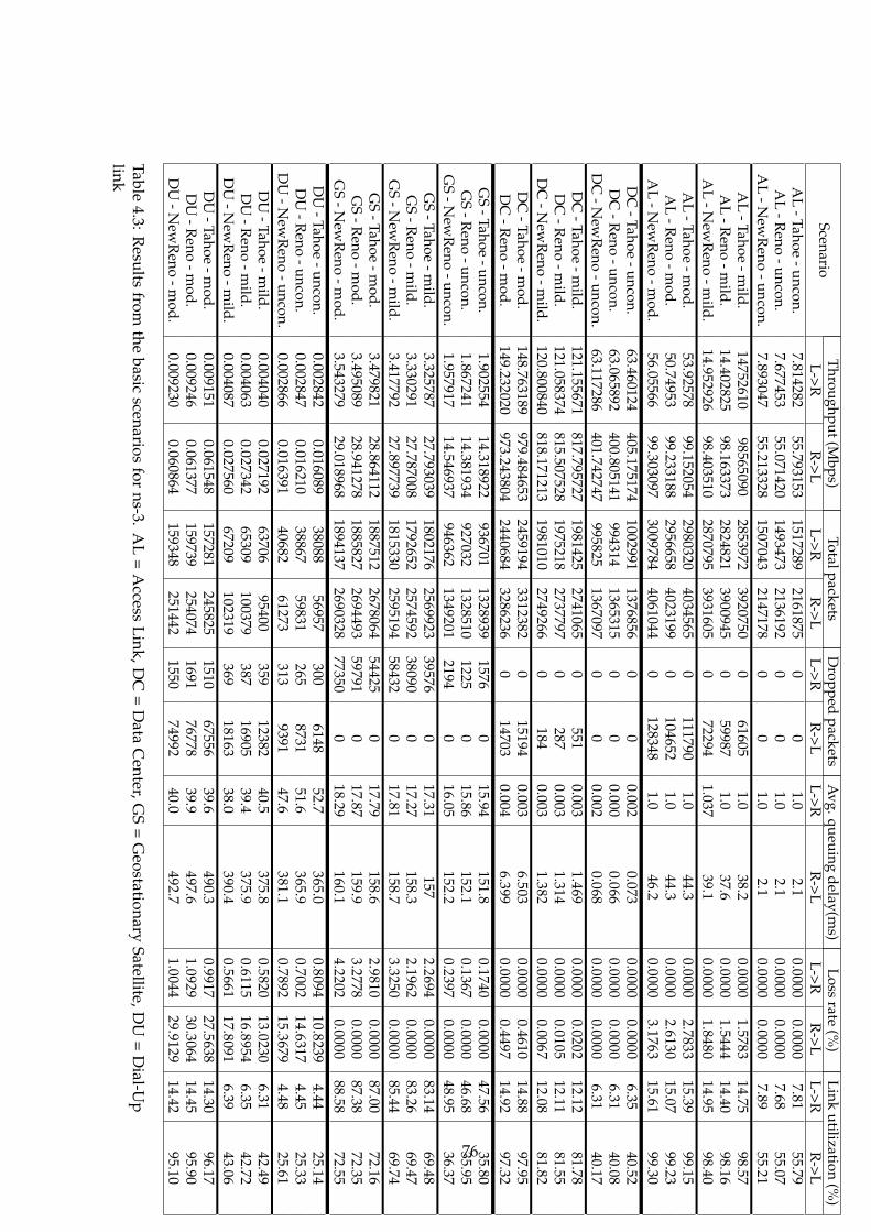
ScenarioT

hroughput(Mbps)

TotalpacketsD

roppedpackets

Avg.queuing

delay(ms)

Lossrate

(%)

Linkutilization

(%)

L->RR

->LL->R

R->L

L->RR

->LL->R

R->L

L->RR

->LL->R

R->L

AL

-Tahoe-uncon.

7.81428255.793153

15172892161875

00

1.02.1

0.00000.0000

7.8155.79

AL

-Reno

-uncon.7.677453

55.0714201493473

21361920

01.0

2.10.0000

0.00007.68

55.07A

L-N

ewR

eno-uncon.

7.89304755.213328

15070432147178

00

1.02.1

0.00000.0000

7.8955.21

AL

-Tahoe-m

ild.14752610

985650902853972

39207500

616051.0

38.20.0000

1.578314.75

98.57A

L-R

eno-m

ild.14.402825

98.1633732824821

39009450

599871.0

37.60.0000

1.544414.40

98.16A

L-N

ewR

eno-m

ild.14.952926

98.4035102870795

39316050

722941.037

39.10.0000

1.848014.95

98.40A

L-Tahoe

-mod.

53.9257899.152054

29803204034565

0111790

1.044.3

0.00002.7833

15.3999.15

AL

-Reno

-mod.

50.7495399.233188

29566584023199

0104652

1.044.3

0.00002.6130

15.0799.23

AL

-New

Reno

-mod.

56.0556699.303097

30097844061044

0128348

1.046.2

0.00003.1763

15.6199.30

DC

-Tahoe-uncon.

63.460124405.175174

10029911376856

00

0.0020.073

0.00000.0000

6.3540.52

DC

-Reno

-uncon.63.065892

400.805141994314

13653150

00.000

0.0660.0000

0.00006.31

40.08D

C-N

ewR

eno-uncon.

63.117286401.742747

9958251367097

00

0.0020.068

0.00000.0000

6.3140.17

DC

-Tahoe-m

ild.121.155671

817.7957271981425

27410650

5510.003

1.4690.0000

0.020212.12

81.78D

C-R

eno-m

ild.121.058374

815.5075281975218

27377970

2870.003

1.3140.0000

0.010512.11

81.55D

C-N

ewR

eno-m

ild.120.800840

818.1712131981010

27492660

1840.003

1.3820.0000

0.006712.08

81.82D

C-Tahoe

-mod.

148.763189979.484653

24591943312382

015194

0.0036.503

0.00000.4610

14.8897.95

DC

-Reno

-mod.

149.232020973.243804

24406843286236

014703

0.0046.399

0.00000.4497

14.9297.32

GS

-Tahoe-uncon.

1.90255414.318922

9367011328939

15760

15.94151.8

0.17400.0000

47.5635.80

GS

-Reno

-uncon.1.867241

14.381934927032

13285101225

015.86

152.10.1367

0.000046.68

35.95G

S-N

ewR

eno-uncon.

1.95791714.546937

9463621349201

21940

16.05152.2

0.23970.0000

48.9536.37

GS

-Tahoe-m

ild.3.325787

27.7930391802176

256992339576

017.31

1572.2694

0.000083.14

69.48G

S-R

eno-m

ild.3.330291

27.7870081792652

257459238090

017.27

158.32.1962

0.000083.26

69.47G

S-N

ewR

eno-m

ild.3.417792

27.8977391815330

259519458432

017.81

158.73.3250

0.000085.44

69.74G

S-Tahoe

-mod.

3.47982128.864112

18875122678064

544250

17.79158.6

2.98100.0000

87.0072.16

GS

-Reno

-mod.

3.49508928.941278

18858272694493

597910

17.87159.9

3.27780.0000

87.3872.35

GS

-New

Reno

-mod.

3.54327929.018968

18941372690328

773500

18.29160.1

4.22020.0000

88.5872.55

DU

-Tahoe-uncon.

0.0028420.016089

3808856957

3006148

52.7365.0

0.809410.8239

4.4425.14

DU

-Reno

-uncon.0.002847

0.01621038867

59831265

873151.6

365.90.7002

14.63174.45

25.33D

U-N

ewR

eno-uncon.

0.0028660.016391

4068261273

3139391

47.6381.1

0.789215.3679

4.4825.61

DU

-Tahoe-m

ild.0.004040

0.02719263706

95400359

1238240.5

375.80.5820

13.02306.31

42.49D

U-R

eno-m

ild.0.004063

0.02734265309

100379387

1690539.4

375.90.6115

16.89546.35

42.72D

U-N

ewR

eno-m

ild.0.004087

0.02756067209

102319369

1816338.0

390.40.5661

17.80916.39

43.06D

U-Tahoe

-mod.

0.0091510.061548

157281245825

151067556

39.6490.3

0.991727.5638

14.3096.17

DU

-Reno

-mod.

0.0092460.061377

159739254074

169176778

39.9497.6

1.092930.3064

14.4595.90

DU

-New

Reno

-mod.

0.0092300.060864

159348251442

155074992

40.0492.7

1.004429.9129

14.4295.10

Table4.3:

Results

fromthe

basicscenarios

forns-3.

AL

=A

ccessLink,D

C=

Data

Center,G

S=

Geostationary

Satellite,DU

=D

ial-Up

link

76

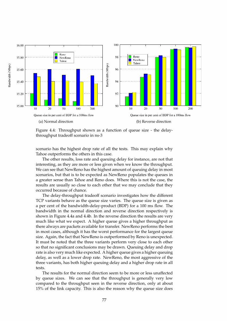
(a) Normal direction (b) Reverse direction

Figure 4.4: Throughput shown as a function of queue size - the delay-throughput tradeoff scenario in ns-3

scenario has the highest drop rate of all the tests. This may explain whyTahoe outperforms the others in this case.

The other results, loss rate and queuing delay for instance, are not thatinteresting, as they are more or less given when we know the throughput.We can see that NewReno has the highest amount of queuing delay in mostscenarios, but that is to be expected as NewReno populates the queues ina greater sense than Tahoe and Reno does. Where this is not the case, theresults are usually so close to each other that we may conclude that theyoccurred because of chance.

The delay-throughput tradeoff scenario investigates how the differentTCP variants behave as the queue size varies. The queue size is given asa per cent of the bandwidth-delay-product (BDP) for a 100 ms flow. Thebandwidth in the normal direction and reverse direction respectively isshown in Figure 4.4a and 4.4b. In the reverse direction the results are verymuch like what we expect. A higher queue gives a higher throughput asthere always are packets available for transfer. NewReno performs the bestin most cases, although it has the worst performance for the largest queuesize. Again, the fact that NewReno is outperformed by Reno is unexpected.It must be noted that the three variants perform very close to each otherso that no significant conclusions may be drawn. Queuing delay and droprate is also very much like expected. A higher queue gives a higher queuingdelay, as well as a lower drop rate. NewReno, the most aggressive of thethree variants, has both higher queuing delay and a higher drop rate in alltests.

The results for the normal direction seem to be more or less unaffectedby queue sizes. We can see that the throughput is generally very lowcompared to the throughput seen in the reverse direction, only at about15% of the link capacity. This is also the reason why the queue size does

77

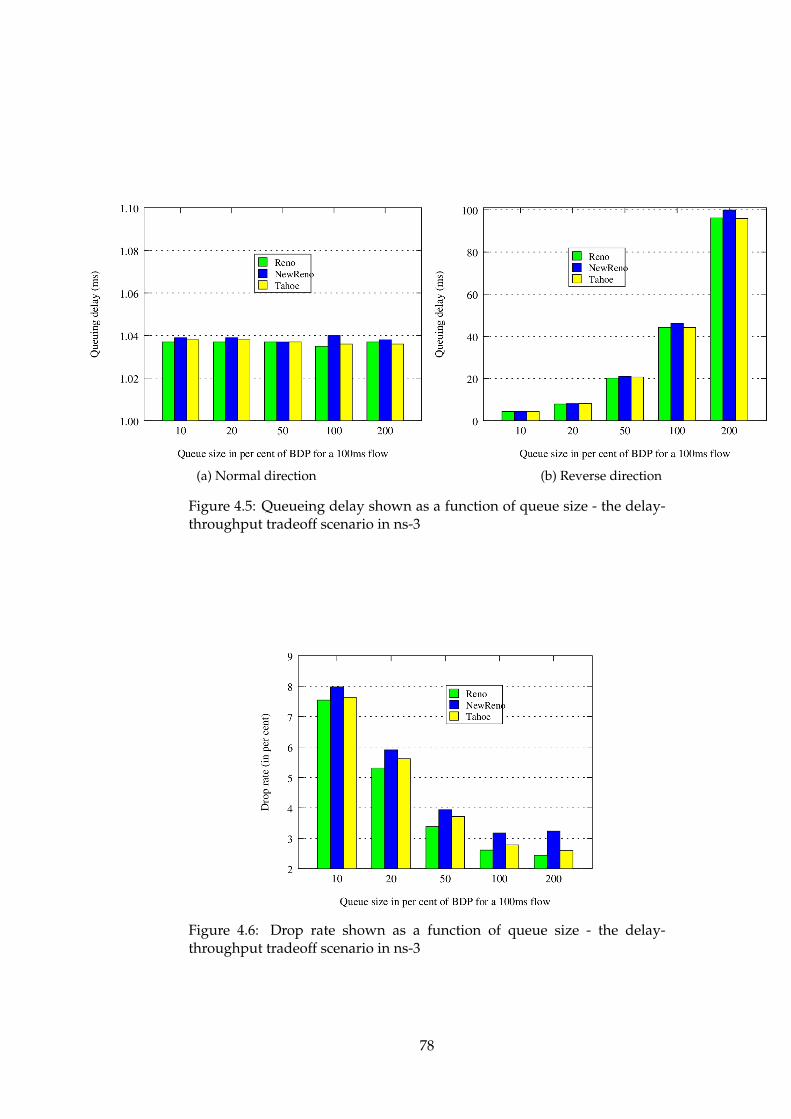
(a) Normal direction (b) Reverse direction

Figure 4.5: Queueing delay shown as a function of queue size - the delay-throughput tradeoff scenario in ns-3

Figure 4.6: Drop rate shown as a function of queue size - the delay-throughput tradeoff scenario in ns-3

78

not really affect the results, because there is always capacity to handle whatlittle traffic is flowing in this direction no matter how small the queue is. Ifthe smallest queue is enough to handle the traffic, then a larger queue willnot really make any difference.

All in all the TCP variants seem to behave according to what we wouldexpect in ns-3.

4.5 OMNeT++ results

The setup for OMNeT++ is the same as for the other scenarios. Eachscenario is run three times with three levels of congestion: uncongested,mild congestion, and moderate congestion. We test three TCP variantsin OMNeT++: Tahoe, Reno and NewReno. We run the same five basicscenarios as in ns-2. The results of these basic scenarios are summarized inTable 4.4 and Table 4.5.

We can see very clearly that these results do not correspond to theexpected results. The three TCP variants all perform more or less exactlythe same. This is seen very clearly in the link utilization columns, wherethe link utilization percentage is rounded. Because it is rounded, the linkutilization is exactly the same in almost every test for the three variants.This should not be the case.

The question we have to try to answer is why these results are so closeto each other. The first thing that came to mind was that we actually failedto switch TCP algorithm, but this does not seem to be the case. There isno randomness involved in these tests, which means that if the same testis run twice, then the results will be exactly the same. Because of this, it isclear that something happens when we change TCP algorithm. Then thereis the question of whether we change the algorithm for only one node, butthis should not be the case either. There is only one line in the configurationfile that decides the TCP algorithm to use, which looks like the followingfor Reno, NewReno and Tahoe respectively:

* * . tcp . tcpAlgorithmClass = "TCPReno"* * . tcp . tcpAlgorithmClass = "TCPNewReno"* * . tcp . tcpAlgorithmClass = " TCPTahoe "

Only one of these is present in the configuration file for each scenariorun, so that there is definitely no problem with precedence of commands.The wildcard notation ’**’ denotes that every single tcp module in thesimulation should use the given tcpAlgorithmClass. We are thereforeconfident that we are in fact running the correct TCP algorithm.

Next we try to consider whether there are scenarios where the threeTCP variants should behave similar to each other. They all share a commonslow start and congestion avoidance phase. The three variants handlepacket drops and retransmissions differently from each other, but if thereare no packet drops, then they should behave exactly the same. In theintuitive sense however, TCP is "greedy", which means that if a TCP senderhas data to send, it will keep increasing its sending rate until a packet

79

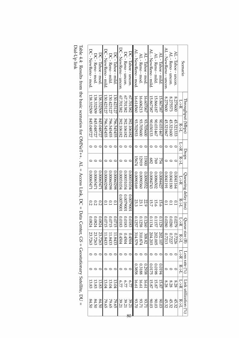
ScenarioT

hroughput(Mbps)

Drops

Queueing

delay(m

s)Q

ueuesize

(B)Loss

rate(%

)Link

utilization(%

)L->R

R->L

L->RR

->LL->R

R->L

L->RR

->LL->R

R->L

L->RR

->LA

L-Tahoe

-uncon.8.275600

45.3213330

00.0041164

0.10.0279

0.72260

08.28

45.32A

L-R

eno-uncon.

8.27557345.321600

00

0.00411800.1

0.02800.7227

00

8.2845.32

AL

-New

Reno

-uncon.8.275600

45.3218670

00.0041191

0.10.0280

0.72130

08.28

45.32A

L-Tahoe

-mild.

15.86738790.031467

0754

0.008442715.6

0.1129202.107

00.0194

15.8790.03

AL

-Reno

-mild.

15.86618790.031467

0769

0.008650215.6

0.1157202.005

00.0198

15.8790.03

AL

-New

Reno

-mild.

15.86738790.030133

0682

0.008474315.7

0.1134204.203

00.0175

15.8790.03

AL

-Tahoe-m

od.16.607067

93.7056000

119000.0090552

22.90.1260

308.820

0.293816.61

93.71A

L-R

eno-m

od.16.606213

93.7056000

129190.0090360

23.10.1258

310.8740

0.318816.61

93.71A

L-N

ewR

eno-m

od.16.614560

93.7029330

156740.0090169

23.30.1257

314.5790

0.385816.61

93.70D

C-Tahoe

-uncon.67.701382

392.1061820

00.00031034

0.00790010.0183

0.45040

06.77

39.21D

C-R

eno-uncon.

67.701382392.106182

00

0.000310340.0079001

0.01830.4504

00

6.7739.21

DC

-New

Reno

-uncon.67.701382

392.1061820

00.00031034

0.00790010.0183

0.45040

06.77

39.21D

C-Tahoe

-mild.

130.423127796.545455

00

0.000602980.1

0.071511.8433

00

13.0479.65

DC

-Reno

-mild.

130.423127796.545455

00

0.000602980.1

0.071511.8433

00

13.0479.65

DC

-New

Reno

-mild.

130.423127796.545455

00

0.000602980.1

0.071511.8433

00

13.0479.65

DC

-Tahoe-m

od.138.332509

845.0487270

00.00065471

0.20.0824

23.72630

013.83

84.50D

C-R

eno-m

od.138.332509

845.0487270

00.00065471

0.20.0824

23.72630

013.83

84.50D

C-N

ewR

eno-m

od.138.332509

845.0487270

00.00065471

0.20.0824

23.72630

013.83

84.50

Table4.4:

Results

fromthe

basicscenarios

forO

MN

eT++.A

L=

Access

Link,DC

=D

ataC

enter,GS

=G

eostationarySatellite,D

U=

Dial-U

plink

80

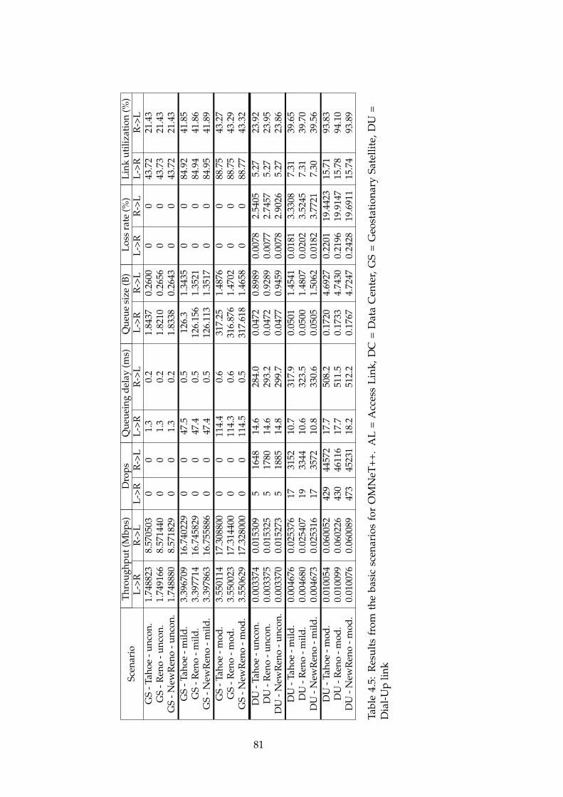
Scen

ario

Thr

ough

put(

Mbp

s)D

rops

Que

uein

gde

lay

(ms)

Que

uesi

ze(B

)Lo

ssra

te(%

)Li

nkut

iliza

tion

(%)

L->R

R->

LL-

>RR

->L

L->R

R->

LL-

>RR

->L

L->R

R->

LL-

>RR

->L

GS

-Tah

oe-u

ncon

.1.

7488

238.

5705

030

01.

30.

21.

8437

0.26

000

043

.72

21.4

3G

S-R

eno

-unc

on.

1.74

9166

8.57

1440

00

1.3

0.2

1.82

100.

2656

00

43.7

321

.43

GS

-New

Ren

o-u

ncon

.1.

7488

808.

5718

290

01.

30.

21.

8338

0.26

430

043

.72

21.4

3G

S-T

ahoe

-mild

.3.

3967

0916

.740

229

00

47.5

0.5

126.

31.

3435

00

84.9

241

.85

GS

-Ren

o-m

ild.

3.39

7714

16.7

4582

90

047

.40.

512

6.15

61.

3521

00

84.9

441

.86

GS

-New

Ren

o-m

ild.

3.39

7863

16.7

5588

60

047

.40.

512

6.11

31.

3517

00

84.9

541

.89

GS

-Tah

oe-m

od.

3.55

0114

17.3

0880

00

011

4.4

0.6

317.

251.

4876

00

88.7

543

.27

GS

-Ren

o-m

od.

3.55

0023

17.3

1440

00

011

4.3

0.6

316.

876

1.47

020

088

.75

43.2

9G

S-N

ewR

eno

-mod

.3.

5506

2917

.328

000

00

114.

50.

531

7.61

81.

4658

00

88.7

743

.32

DU

-Tah

oe-u

ncon

.0.

0033

740.

0153

095

1648

14.6

284.

00.

0472

0.89

890.

0078

2.54

055.

2723

.92

DU

-Ren

o-u

ncon

.0.

0033

750.

0153

255

1780

14.6

293.

20.

0472

0.92

890.

0077

2.74

575.

2723

.95

DU

-New

Ren

o-u

ncon

.0.

0033

700.

0152

735

1885

14.8

299.

70.

0477

0.94

590.

0078

2.90

265.

2723

.86

DU

-Tah

oe-m

ild.

0.00

4676

0.02

5376

1731

5210

.731

7.9

0.05

011.

4541

0.01

813.

3308

7.31

39.6

5D

U-R

eno

-mild

.0.

0046

800.

0254

0719

3344

10.6

323.

50.

0500

1.48

070.

0202

3.52

457.

3139

.70

DU

-New

Ren

o-m

ild.

0.00

4673

0.02

5316

1735

7210

.833

0.6

0.05

051.

5062

0.01

823.

7721

7.30

39.5

6D

U-T

ahoe

-mod

.0.

0100

540.

0600

5242

944

572

17.7

508.

20.

1720

4.69

270.

2201

19.4

423

15.7

193

.83

DU

-Ren

o-m

od.

0.01

0099

0.06

0226

430

4611

617

.751

1.5

0.17

334.

7430

0.21

9619

.914

715

.78

94.1

0D

U-N

ewR

eno

-mod

.0.

0100

760.

0600

8947

345

231

18.2

512.

20.

1767

4.72

470.

2428

19.6

911

15.7

493

.89

Tabl

e4.

5:R

esul

tsfr

omth

eba

sic

scen

ario

sfo

rO

MN

eT++

.A

L=

Acc

ess

Link

,DC

=D

ata

Cen

ter,

GS

=G

eost

atio

nary

Sate

llite

,DU

=D

ial-

Up

link

81

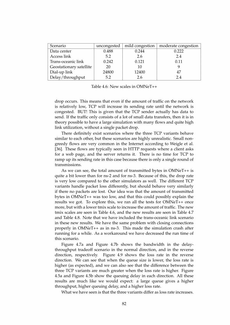
Scenario uncongested mild congestion moderate congestionData center 0.488 0.244 0.222Access link 5.2 2.6 2.4Trans-oceanic link 0.242 0.121 0.11Geostationary satellite 20 10 9Dial-up link 24800 12400 47Delay/throughput 5.2 2.6 2.4

Table 4.6: New scales in OMNeT++

drop occurs. This means that even if the amount of traffic on the networkis relatively low, TCP will increase its sending rate until the network iscongested. BUT! This is given that the TCP sender actually has data tosend. If the traffic only consists of a lot of small data transfers, then it is intheory possible to have a large simulation with many flows and quite highlink utilization, without a single packet drop.

There definitely exist scenarios where the three TCP variants behavesimilar to each other, but these scenarios are highly unrealistic. Small non-greedy flows are very common in the Internet according to Weigle et al.[36]. These flows are typically seen in HTTP requests where a client asksfor a web page, and the server returns it. There is no time for TCP toramp up its sending rate in this case because there is only a single round oftransmissions.

As we can see, the total amount of transmitted bytes in OMNeT++ isquite a bit lower than for ns-2 and for ns-3. Because of this, the drop rateis very low compared to the other simulators as well. The different TCPvariants handle packet loss differently, but should behave very similarlyif there no packets are lost. Our idea was that the amount of transmittedbytes in OMNeT++ was too low, and that this could possibly explain theresults we got. To explore this, we ran all the tests for OMNeT++ oncemore, but with a lower tmix scale to increase the amount of traffic. The newtmix scales are seen in Table 4.6, and the new results are seen in Table 4.7and Table 4.8. Note that we have included the trans-oceanic link scenarioin these new results. We have the same problem with closing connectionsproperly in OMNeT++ as in ns-3. This made the simulation crash afterrunning for a while. As a workaround we have decreased the run time ofthis scenario.

Figure 4.7a and Figure 4.7b shows the bandwidth in the delay-throughput tradeoff scenario in the normal direction, and in the reversedirection, respectively. Figure 4.9 shows the loss rate in the reversedirection. We can see that when the queue size is lower, the loss rate ishigher (as expected), and we can also see that the difference between thethree TCP variants are much greater when the loss rate is higher. Figure4.5a and Figure 4.5b show the queuing delay in each direction. All theseresults are much like we would expect: a large queue gives a higherthroughput, higher queuing delay, and a higher loss rate.

What we have seen is that the three variants differ as loss rate increases.

82

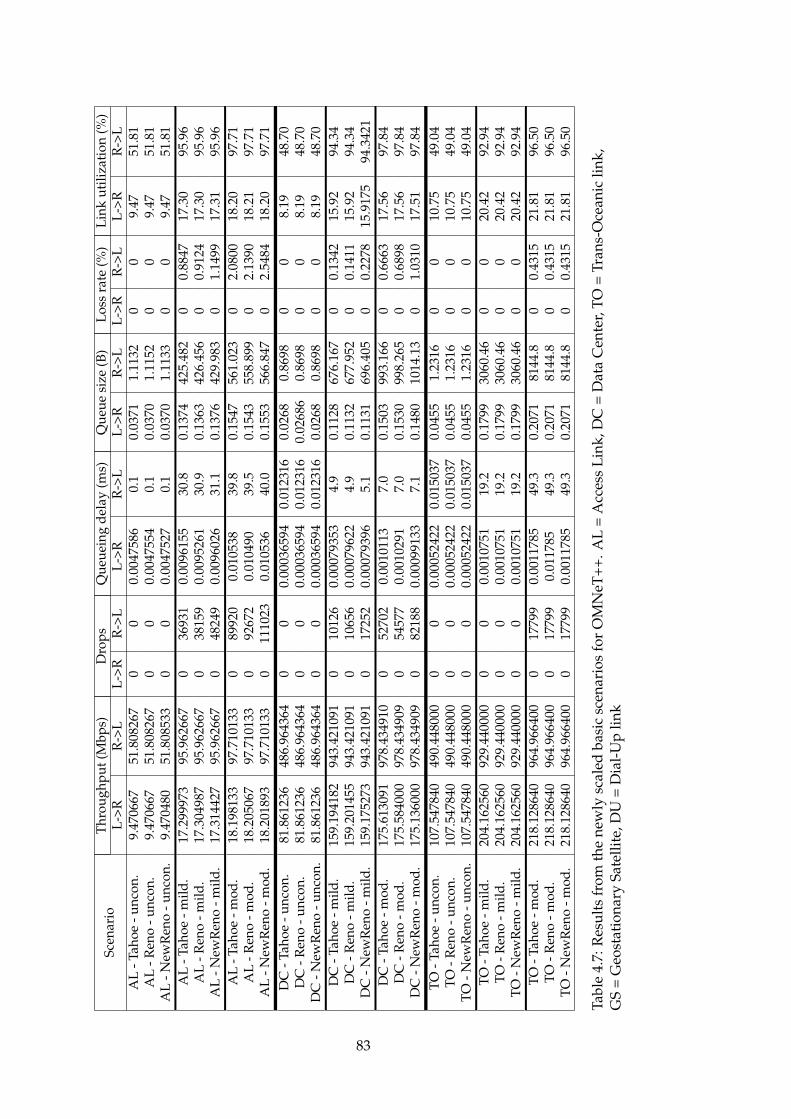
Scen

ario

Thro

ughp

ut(M

bps)

Dro

psQ

ueue

ing

dela

y(m

s)Q

ueue

size

(B)

Loss

rate

(%)

Link

utili

zati

on(%

)L-

>RR

->L

L->R

R->

LL-

>RR

->L

L->R

R->

LL-

>RR

->L

L->R

R->

LA

L-T

ahoe

-unc

on.

9.47

0667

51.8

0826

70

00.

0047

586

0.1

0.03

711.

1132

00

9.47

51.8

1A

L-R

eno

-unc

on.

9.47

0667

51.8

0826

70

00.

0047

554

0.1

0.03

701.

1152

00

9.47

51.8

1A

L-N

ewR

eno

-unc

on.

9.47

0480

51.8

0853

30

00.

0047

527

0.1

0.03

701.

1133

00

9.47

51.8

1A

L-T

ahoe

-mild

.17

.299

973

95.9

6266

70

3693

10.

0096

155

30.8

0.13

7442

5.48

20

0.88

4717

.30

95.9

6A

L-R

eno

-mild

.17

.304

987

95.9

6266

70

3815

90.

0095

261

30.9

0.13

6342

6.45

60

0.91

2417

.30

95.9

6A

L-N

ewR

eno

-mild

.17

.314

427

95.9

6266

70

4824

90.

0096

026

31.1

0.13

7642

9.98

30

1.14

9917

.31

95.9

6A

L-T

ahoe

-mod

.18

.198

133

97.7

1013

30

8992

00.

0105

3839

.80.

1547

561.

023

02.

0800

18.2

097

.71

AL

-Ren

o-m

od.

18.2

0506

797

.710

133

092

672

0.01

0490

39.5

0.15

4355

8.89

90

2.13

9018

.21

97.7

1A

L-N

ewR

eno

-mod

.18

.201

893

97.7

1013

30

1110

230.

0105

3640

.00.

1553

566.

847

02.

5484

18.2

097

.71

DC

-Tah

oe-u

ncon

.81

.861

236

486.

9643

640

00.

0003

6594

0.01

2316

0.02

680.

8698

00

8.19

48.7

0D

C-R

eno

-unc

on.

81.8

6123

648

6.96

4364

00

0.00

0365

940.

0123

160.

0268

60.

8698

00

8.19

48.7

0D

C-N

ewR

eno

-unc

on.

81.8

6123

648

6.96

4364

00

0.00

0365

940.

0123

160.

0268

0.86

980

08.

1948

.70

DC

-Tah

oe-m

ild.

159.

1941

8294

3.42

1091

010

126

0.00

0793

534.

90.

1128

676.

167

00.

1342

15.9

294

.34

DC

-Ren

o-m

ild.

159.

2014

5594

3.42

1091

010

656

0.00

0796

224.

90.

1132

677.

952

00.

1411

15.9

294

.34

DC

-New

Ren

o-m

ild.

159.

1752

7394

3.42

1091

017

252

0.00

0793

965.

10.

1131

696.

405

00.

2278

15.9

175

94.3

421

DC

-Tah

oe-m

od.

175.

6130

9197

8.43

4910

052

702

0.00

1011

37.

00.

1503

993.

166

00.

6663

17.5

697

.84

DC

-Ren

o-m

od.

175.

5840

0097

8.43

4909

054

577

0.00

1029

17.

00.

1530

998.

265

00.

6898

17.5

697

.84

DC

-New

Ren

o-m

od.

175.

1360

0097

8.43

4909

082

188

0.00

0991

337.

10.

1480

1014

.13

01.

0310

17.5

197

.84

TO-T

ahoe

-unc

on.

107.

5478

4049

0.44

8000

00

0.00

0524

220.

0150

370.

0455

1.23

160

010

.75

49.0

4TO

-Ren

o-u

ncon

.10

7.54

7840

490.

4480

000

00.

0005

2422

0.01

5037

0.04

551.

2316

00

10.7

549

.04

TO-N

ewR

eno

-unc

on.

107.

5478

4049

0.44

8000

00

0.00

0524

220.

0150

370.

0455

1.23

160

010

.75

49.0

4TO

-Tah

oe-m

ild.

204.

1625

6092

9.44

0000

00

0.00

1075

119

.20.

1799

3060

.46

00

20.4

292

.94

TO-R

eno

-mild

.20

4.16

2560

929.

4400

000

00.

0010

751

19.2

0.17

9930

60.4

60

020

.42

92.9

4TO

-New

Ren

o-m

ild.

204.

1625

6092

9.44

0000

00

0.00

1075

119

.20.

1799

3060

.46

00

20.4

292

.94

TO-T

ahoe

-mod

.21

8.12

8640

964.

9664

000

1779

90.

0011

785

49.3

0.20

7181

44.8

00.

4315

21.8

196

.50

TO-R

eno

-mod

.21

8.12

8640

964.

9664

000

1779

90.

0117

8549

.30.

2071

8144

.80

0.43

1521

.81

96.5

0TO

-New

Ren

o-m

od.

218.

1286

4096

4.96

6400

017

799

0.00

1178

549

.30.

2071

8144

.80

0.43

1521

.81

96.5

0

Tabl

e4.

7:R

esul

tsfr

omth

ene

wly

scal

edba

sic

scen

ario

sfo

rO

MN

eT++

.AL

=A

cces

sLi

nk,D

C=

Dat

aC

ente

r,TO

=Tr

ans-

Oce

anic

link,

GS

=G

eost

atio

nary

Sate

llite

,DU

=D

ial-

Up

link

83

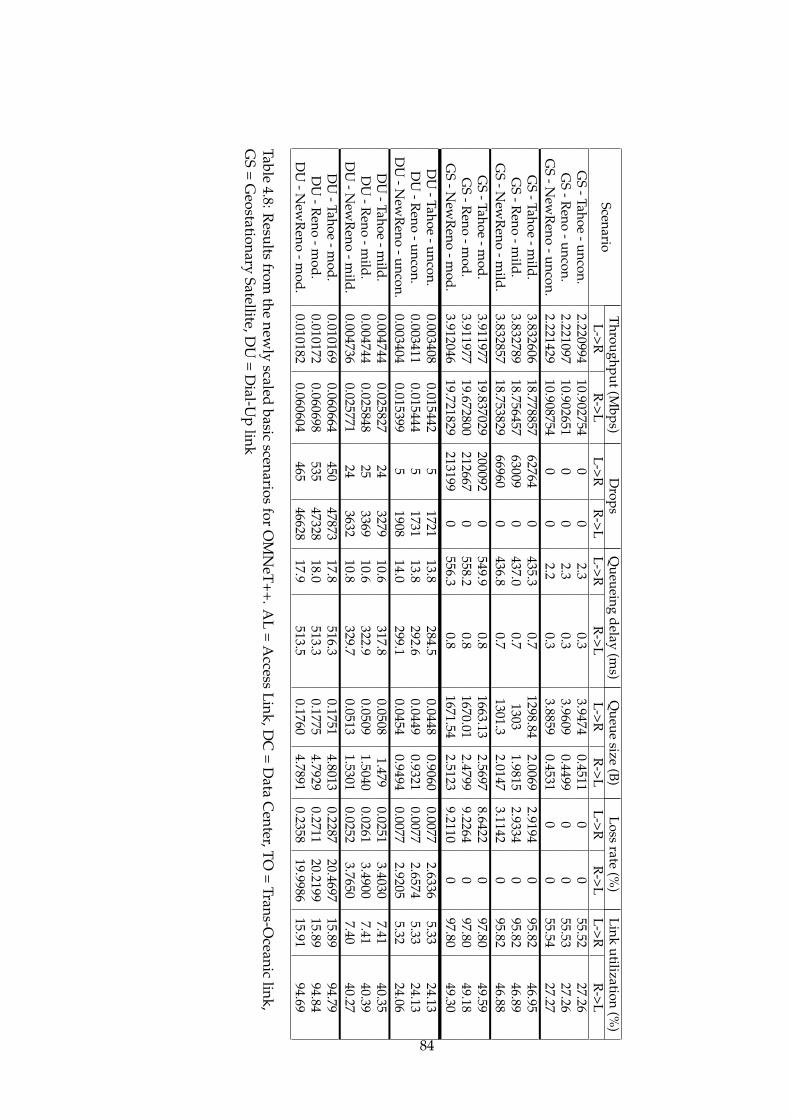
ScenarioThroughput(M

bps)D

ropsQ

ueueingdelay

(ms)

Queue

size(B)

Lossrate

(%)

Linkutilization

(%)

L->RR

->LL->R

R->L

L->RR

->LL->R

R->L

L->RR

->LL->R

R->L

GS

-Tahoe-uncon.

2.22099410.902754

00

2.30.3

3.94740.4511

00

55.5227.26

GS

-Reno

-uncon.2.221097

10.9026510

02.3

0.33.9609

0.44990

055.53

27.26G

S-N

ewR

eno-uncon.

2.22142910.908754

00

2.20.3

3.88590.4531

00

55.5427.27

GS

-Tahoe-m

ild.3.832606

18.77885762764

0435.3

0.71298.84

2.00692.9194

095.82

46.95G

S-R

eno-m

ild.3.832789

18.75645763009

0437.0

0.71303

1.98152.9334

095.82

46.89G

S-N

ewR

eno-m

ild.3.832857

18.75382966960

0436.8

0.71301.3

2.01473.1142

095.82

46.88G

S-Tahoe

-mod.

3.91197719.837029

2000920

549.90.8

1663.132.5697

8.64220

97.8049.59

GS

-Reno

-mod.

3.91197719.672800

2126670

558.20.8

1670.012.4799

9.22640

97.8049.18

GS

-New

Reno

-mod.

3.91204619.721829

2131990

556.30.8

1671.542.5123

9.21100

97.8049.30

DU

-Tahoe-uncon.

0.0034080.015442

51721

13.8284.5

0.04480.9060

0.00772.6336

5.3324.13

DU

-Reno

-uncon.0.003411

0.0154445

173113.8

292.60.0449

0.93210.0077

2.65745.33

24.13D

U-N

ewR

eno-uncon.

0.0034040.015399

51908

14.0299.1

0.04540.9494

0.00772.9205

5.3224.06

DU

-Tahoe-m

ild.0.004744

0.02582724

327910.6

317.80.0508

1.4790.0251

3.40307.41

40.35D

U-R

eno-m

ild.0.004744

0.02584825

336910.6

322.90.0509

1.50400.0261

3.49007.41

40.39D

U-N

ewR

eno-m

ild.0.004736

0.02577124

363210.8

329.70.0513

1.53010.0252

3.76507.40

40.27D

U-Tahoe

-mod.

0.0101690.060664

45047873

17.8516.3

0.17514.8013

0.228720.4697

15.8994.79

DU

-Reno

-mod.

0.0101720.060698

53547328

18.0513.3

0.17754.7929

0.271120.2199

15.8994.84

DU

-New

Reno

-mod.

0.0101820.060604

46546628

17.9513.5

0.17604.7891

0.235819.9986

15.9194.69

Table4.8:R

esultsfrom

thenew

lyscaled

basicscenarios

forO

MN

eT++.AL

=A

ccessLink,D

C=

Data

Center,TO

=Trans-O

ceaniclink,

GS

=G

eostationarySatellite,D

U=

Dial-U

plink

84

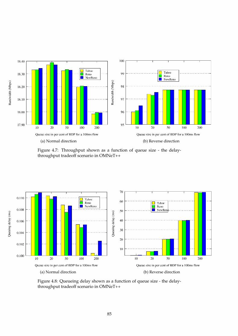
(a) Normal direction (b) Reverse direction

Figure 4.7: Throughput shown as a function of queue size - the delay-throughput tradeoff scenario in OMNeT++

(a) Normal direction (b) Reverse direction

Figure 4.8: Queueing delay shown as a function of queue size - the delay-throughput tradeoff scenario in OMNeT++

85

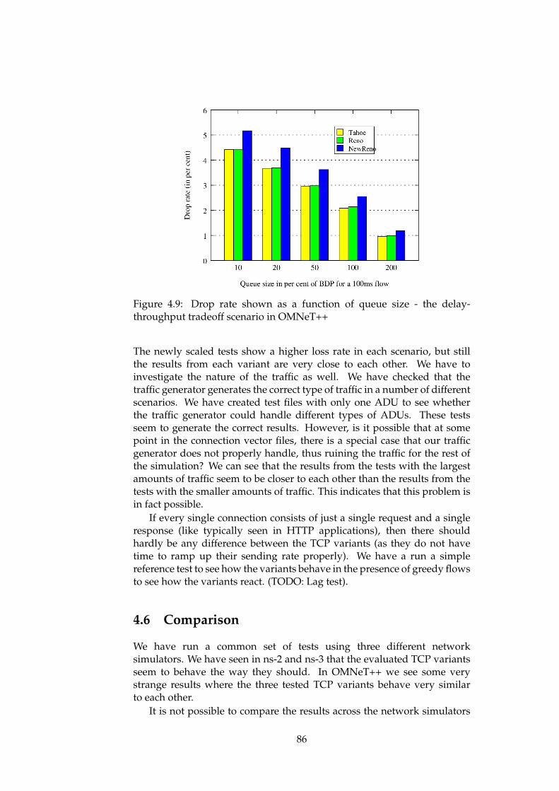
Figure 4.9: Drop rate shown as a function of queue size - the delay-throughput tradeoff scenario in OMNeT++

The newly scaled tests show a higher loss rate in each scenario, but stillthe results from each variant are very close to each other. We have toinvestigate the nature of the traffic as well. We have checked that thetraffic generator generates the correct type of traffic in a number of differentscenarios. We have created test files with only one ADU to see whetherthe traffic generator could handle different types of ADUs. These testsseem to generate the correct results. However, is it possible that at somepoint in the connection vector files, there is a special case that our trafficgenerator does not properly handle, thus ruining the traffic for the rest ofthe simulation? We can see that the results from the tests with the largestamounts of traffic seem to be closer to each other than the results from thetests with the smaller amounts of traffic. This indicates that this problem isin fact possible.

If every single connection consists of just a single request and a singleresponse (like typically seen in HTTP applications), then there shouldhardly be any difference between the TCP variants (as they do not havetime to ramp up their sending rate properly). We have a run a simplereference test to see how the variants behave in the presence of greedy flowsto see how the variants react. (TODO: Lag test).

4.6 Comparison

We have run a common set of tests using three different networksimulators. We have seen in ns-2 and ns-3 that the evaluated TCP variantsseem to behave the way they should. In OMNeT++ we see some verystrange results where the three tested TCP variants behave very similarto each other.

It is not possible to compare the results across the network simulators

86

however, as the numbers are quite far off. If the evaluation suite wasmodelled perfectly in all three simulators, we could draw the conclusionthat at least two of three network simulators do not function as they should.However the problem is that there is quite a bit of uncertainty in a numberof things, and especially in the traffic generator, so that we cannot drawsuch a conclusion. In this section we consider a few details in which wehave been uncertain and discuss the significance of these details.

For each pair of communicating initiator/acceptor pair in the simu-lation, there is a connection vector file describing the traffic. We havetried combining different files with different node-pairs, but this has notchanged the results significantly. We are confident that we now use thesame connection vector file in each of the three simulators to describe thetraffic between the same initiator/acceptor pair.

There are quite a few options in the configuration of TCP. We havemostly used the default values unless otherwise described in the evaluationsuite. Delayed acks, selective acknowledgements (SACK), window scaling,and timestamp support is disabled by default. Nagle’s algorithm is enabledfor ns-2 and OMNeT++, but is not supported in ns-3. These options shouldbe mostly equal for every simulator. We also know that OMNeT++ isdifferent from ns-2 and ns-3 because the OMNeT++ version of tmix ignoresthe initial congestion window size specified in the connection vector files.To see the effect of setting the correct initial congestion window size, wehave run a few of the scenarios in ns-3 without this functionality to seehow it affects the results. We have run the dial-up basic scenario with allcongestion levels, and we have also run the access link uncongested. Theresults are seen in Table 4.9 and we have included parts of the originalresults in Table 4.10 as well so that they are easier to compare. Whatwe can see in these results is that the new results have a slightly lowerthroughput, and the new results are also slightly closer to each other thanthe original results. These numbers are, however, not like the results wesee in OMNeT++, so we can conclude that the initial congestion windowsize functionality in itself is not the reason for why the OMNeT++ resultsare strange.

The most likely culprit in this case is the traffic generator. There is alarge difference between the results from the different simulators. This canprobably not be explained by small differences such as TCP options andsuch. A difference in how the traffic generator works may have the sort ofimpact that we see in our results.

4.7 Discussion

In the beginning of this thesis we were focused on trying to verify, or at leastexplore, the realism of network simulators. We chose the TCP evaluationsuite as a basis for our test cases. As the thesis has progressed, the focushas shifted more and more from the verification of network simulators, toworking on the TCP evaluation suite, and as a consequence, the tmix trafficgenerator.

87

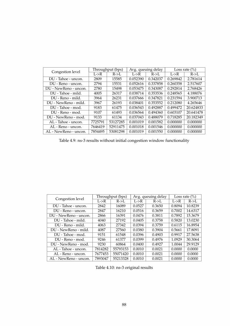
Congestion level Throughput (bps) Avg. queuing delay Loss rate (%)L->R R->L L->R R->L L->R R->L

DU - Tahoe - uncon. 2809 15585 0.052390 0.342037 0.269842 2.781614DU - Reno - uncon. 2794 15531 0.052616 0.337858 0.260358 2.517607

DU - NewReno - uncon. 2780 15498 0.053475 0.343087 0.292814 2.768426DU - Tahoe - mild. 4005 26317 0.038714 0.353536 0.248565 4.188076DU - Reno - mild. 3964 26231 0.037666 0.347821 0.231594 3.900713

DU - NewReno - mild. 3967 26193 0.038401 0.353552 0.212080 4.265646DU - Tahoe - mod. 9183 61475 0.036543 0.492887 0.499472 20.624833DU - Reno - mod. 9107 61493 0.036564 0.494360 0.603107 20.641478

DU - NewReno - mod. 9133 61134 0.037043 0.488079 0.718285 20.182349AL - Tahoe - uncon. 7725791 53127285 0.001019 0.001582 0.000000 0.000000AL - Reno - uncon. 7646419 52911475 0.001018 0.001546 0.000000 0.000000

AL - NewReno - uncon. 7854495 53081298 0.001019 0.001550 0.000000 0.000000

Table 4.9: ns-3 results without initial congestion window functionality

Congestion level Throughput (bps) Avg. queuing delay Loss rate (%)L->R R->L L->R R->L L->R R->L

DU - Tahoe - uncon. 2842 16089 0.0527 0.3650 0.8094 10.8239DU - Reno - uncon. 2847 16210 0.0516 0.3659 0.7002 14.6317

DU - NewReno - uncon. 2866 16391 0.0476 0.3811 0.7892 15.3679DU - Tahoe - mild. 4040 27192 0.0405 0.3758 0.5820 13.0230DU - Reno - mild. 4063 27342 0.0394 0.3759 0.6115 16.8954

DU - NewReno - mild. 4087 27560 0.0380 0.3904 0.5661 17.8091DU - Tahoe - mod. 9151 61548 0.0396 0.4903 0.9917 27.5638DU - Reno - mod. 9246 61377 0.0399 0.4976 1.0929 30.3064

DU - NewReno - mod. 9230 60864 0.0400 0.4927 1.0044 29.9129AL - Tahoe - uncon. 7814282 55793153 0.0010 0.0021 0.0000 0.0000AL - Reno - uncon. 7677453 55071420 0.0010 0.0021 0.0000 0.0000

AL - NewReno - uncon. 7893047 55213328 0.0010 0.0021 0.0000 0.0000

Table 4.10: ns-3 original results

88

The TCP evaluation suite seemed like a good basis for evaluating theTCP functionality of each network simulator. The problem with the suitehowever was that it was a work in progress (and still is). The draft that wegot from David Hayes was exactly that, a draft. This means that at severalpoints, the suite is very unclear, which has made it difficult to work with attimes.

Another big problem with choosing the TCP evaluation suite for ourcomparison of network simulators has been the traffic generation. Tmix isa very complex traffic generator, which makes it difficult to validate ourresults in general. How can we compare the results of ns-2, ns-3, andOMNeT++ if we cannot with absolute certainty claim that tmix works asintended? In talks with David we have learned that when they working onthe evaluation suite in ns-2, they had a lot of trouble with tmix, and theyhad to make several improvements on it before they were able to use it intheir suite. In this thesis we have also struggled a lot with tmix, both in ns-3,and in OMNeT++. We can conclude that when comparing simulators, tmixhas been an unnecessarily complicating factor. To compare the simulators,a simpler traffic generator that would be easier to reproduce in all threesimulators would have been a better choice.

4.7.1 Tmix

Through the work in this thesis, we have some thoughts on tmix as a trafficgenerator. First of all, tmix is a traffic generator that generates traffic basedon connections described in a connection vector file. This means that thetraffic not only depends on the generator itself, but also on the traces.

As mentioned above, we have scenarios where the average linkutilization is 80%, but there still is not a single packet drop. This is verystrange. One would think that even if the level of traffic is relatively low,TCP would still increase its sending rate in such a way that packet dropswould occur. Because of this we would see a difference in the behaviourof Tahoe, Reno, and NewReno even though the level of traffic was low.However if there are no greedy flows, i.e., a flow that actually needs a highamount of bandwidth, and there are quite a few non-greedy flows, then itis in theory possible to have a high link utilization and no packet loss.

In real life, there is no such thing a real greedy flow, i.e., a flow thatalways tries to hog as much of the network resources as possible, but thereare flows that are greedy in the more intuitive sense over a short amountof time. For instance the transfer of a 1GB file will act like a greedy flowfor a while in a network with low capacity like 1Mbps. In this case, theTCP sender will try to hog as much of the capacity as possible for a longtime. However, if we increase the network capacity to 10Gbps, then thistransfer is not really greedy in the intuitive sense anymore, as there is morethan enough capacity to transfer the file in a relative short amount of time,while still leaving network resources available for other flows.

This is part of what we think is the problem with tmix. Considerthe creation of a connection vector file. To create the connection vectorfiles, a tmix observer is placed somewhere in the network (preferably at

89

some bottleneck node of some sort). All the traffic that flows throughthis observer is saved in connection vector files, so that the traffic can bereproduced at a later point. Now consider what happens when a TCPsender wants to send a file larger than the maximum transmission unit(MTU), for instance 10MB. The TCP sender will split the file into severalsmaller segments. A typical MTU is 1500 bytes, with 40 bytes reservedfor the TCP and IP headers. 10MB / 1500B give us 6850 packets. Nowconsider the network capacity to be 8Mbps. If we ignore the slow startand congestion avoidance algorithm for now, it should take 10 secondsto complete this transfer, where each packet arrives with an interval ofroughly 1.5ms. If we try to replay this connection vector file in a similarnetwork, then the traffic that tmix generates will look much like the trafficin the original network. It will look like a connection that is "greedy"for 10 seconds. Now what happens if we increase the capacity of thenetwork? The problem is that the connection vector does not adapt to thenew network. If we were to transfer 10MB in a higher capacity network,there would still be 6850 packets (given that the MTU is still the same), butthe time between each of them would be much lower. Tmix does not reflectthis.

The general problem here is that it is very difficult when observinga network to know whether a single packet is just a part of a largeApplication Data Unit (ADU), or whether it is an actual ADU in itself.In the previous example, the observer cannot know whether each ofthe packets observed are all part of a large ADU, or whether they areall individual smaller ADUs. When increasing the network capacity,there no longer exist any greedy flows in the connection vector files asthe connection vector files are limited by the network where the tracewas created. Traffic may be scaled by concentrating the arrival rate ofconnections, and as such it is possible to get congestion in the network, butit is also possible to get high network utilization, while still never droppingpackets as there are no greedy flows.

Another problem with tmix is that it does not react to the state of thenetwork. As the network congestion increases, TCP will back off to tryto avoid a network collapse, but this is not the only thing that happensin real networks. For instance consider the users that surf the web orstream movies. What happens when packets are dropped repeatedly andthe performance of the network stoops? A user might decide to watch themovie at a later time, or the user might give up on a web page that loadstoo slowly.

Even though tmix does not necessarily react exactly like the real worldwould as the network changes, it does not mean that tmix is useless as atool to generate traffic. The traffic does have certain attributes from the realworld, and the nature of the traffic is similar to traffic observed in the realworld. We feel however that we are missing a few details, for instance thepossibility of identifying greedy flows. It must be noted that it is easy toinsert manually created connection vectors into the connection vector filesthat are greedy.

90

Chapter 5

Conclusion

The idea of this thesis was to try to investigate the TCP implementationof several commonly used network simulators to try to figure out whetherthey function like they are supposed to, i.e., as described in their respectiveRFCs, and also as seen in other research. There have been several problemshowever with this comparison, and the focus of this thesis has shifted moreand more towards working with the TCP evaluation suite, rather thanactually verifying the simulators.

We have implemented a subset of the tests described in the TCPevaluation suite in ns-3 and in OMNeT++. The reason for why we have notimplemented the entire suite is partly because of the time constraint of thisthesis, but also because we were getting a good indication of the results wecould expect from only running the subset that we have implemented. Wehave compared these results to the ns-2 version of the suite. In additionto implementing the tests in each simulator, we have also created thetmix traffic generator in OMNeT++, as well as improved the tmix trafficgenerator in ns-3.

We have a number of results from ns-2, ns-3, and OMNeT++. In theresults from ns-2 and ns-3 we can see the type of behaviour one wouldexpect to see in the TCP variants that we have tested. The results fromour OMNeT++ simulations do not show this kind of behaviour. If wecompare the results from one simulator with the results of the others, wecan see that the numbers deviate by quite a lot. Unfortunately, we cannotdraw any conclusion to whether the simulators behave in the way theyshould for a number of reasons. The results stem from the same suiteof tests, from the TCP evaluation suite. The TCP evaluation suite is veryimmature and is a work in progress. This fact has led to a bit of uncertaintywhen implementing the suite, which may have led to differences in thethree simulator implementations. Another complicating factor has been thetraffic generator tmix. We have worked a lot on making tmix work properlyfor ns-3, and we have also implemented this traffic generator from scratchin OMNeT++. Because our results deviate as much as they do, we believethat only element in the suite that may explain such a deviation is the trafficgenerator, which seems to have problems in its implementation. Becauseof this, we believe that the main cause of the differences we observe in the

91

three network simulators is caused by the traffic generator. As we suspectthat tmix is not functioning identically in all three simulators, we cannotdraw any conclusion to whether the simulators behave like the real world.

Even though we cannot verify the simulators, we have still worked alot with the three network simulators, the TCP evaluation suite and tmix,and we do have some observations regarding these.

OMNeT++ is very limited in its TCP functionality. OMNeT++ hasTahoe, Reno, and NewReno, as well as TCP without congestion controlbuilt-in in the simulator. In addition to the built-in TCP algorithms,OMNeT++ also has added support for the Network Simulation Cradle(NSC) that makes it possible to run real world protocol stacks. The supportfor NSC is still very limited in OMNeT++. It only supports the Linux stackand the lightweight IP (lwIP) stack at the moment. We have not used lwIP,but we tried to use the Linux stack. NSC comes with a few limitations thatmake it difficult to use with tmix. For instance, it is not possible to changethe maximum segment size (MSS), and it only supports the bytestreamtransfer mode, while tmix uses the object transfer mode.

ns-3 is also rather limited in its TCP functionality. ns-3, as OMNeT++,has built-in support for Tahoe, Reno and NewReno, as well as TCP withoutcongestion control. There is no support for selective acknowledgements(SACK) or Nagle’s algorithm. These three very basic TCP algorithmswithout support for SACK make for a very limited TCP functionality inns-3. In addition to the TCP algorithms however, ns-3 also supports NSC.NSC in ns-3 has its limitations as well. First of all it only supports Linuxstacks, and it has some other limitations as well, such as the fact that NSConly works on single-interface nodes. We were unable to run NSC in thisthesis because NSC crashed in almost every single simulation except forthe really short-running ones (the dial-up link scenario). NSC in ns-3 is stilla work in progress however, and we will probably see improvements in thefuture.

ns-2 is very rich in its TCP functionality compared to ns-3 andOMNeT++. ns-2 has built-in support for the more basic TCP variants suchas Tahoe, Reno and NewReno, but it also has built-in all the variants foundin the Linux kernel, which includes for instance Westwood, BIC, CUBICand Hybla. In addition to the built-in variants, it is also possible to run theNSC in ns-2 (actually, NSC was built for ns-2), and has no limitations likethe ones seen in ns-3 and OMNeT++ as far as we know.

We have, as far as we know, been the first to try the suite in practice, andin our opinion it is not ready yet. While the idea of creating a standardizedtest suite to evaluate TCP is a good one, there is still room for improvementin the current state of the suite.

One problem with the suite is the way that it defines congestion.Congestion is simply defined as an average drop rate. For instance, ascenario is defined to be moderately congested when the average lossrate of the simulation meets a certain value. The problem with definingcongestion in this way is that the TCP streams are constantly on the edge ofcollapsing, which makes them very unstable. In short simulation runs it ispossible to find a level of traffic so that the average loss rate meets the target

92

loss rate. In long simulation runs however, it is very difficult to maintain alevel of congestion without the network collapsing at some point. Anotherproblem with this way of defining congestion is that each TCP variantbehaves differently, making it impossible for every TCP variant to meetthe target loss rate at the same time. The evaluation suite is very vague atthis point.

Another concern we have for the TCP evaluation suite is the way thattraffic is generated. At the moment the tmix traffic generator is used. Tmixis based on network traces from real networks, and is thus realistic in thatsense. We argue however, that when the network changes (for instance ifwe increase the capacity of the network), the traffic generated by tmix doesnot reflect this. We believe that the traffic generated by tmix is limited bythe network in which the traces were captured.

5.1 Future work

Both ns-3 and OMNeT++ are very limited when it comes to TCP. We believethat once NSC is properly in place, this will improve. Then there is alsothe question of whether the simulators act the way that they should. Wehave found several unexpected results in our simulations that could befurther explored, for instance, why does Reno in some cases outperformNewReno?

We have also worked quite a bit with the tmix traffic generator. Oneof the problems with generating traffic from trace sources is that it isvery difficult when observing a network to reverse engineer what theapplication was originally doing. For instance, when a client requestsa large file, the observer will see a steady stream of smaller segmentedpackets coming from the server, but there is no way for the observer toknow what the original request looked like. This is seen clearly in tmix.Tmix will reproduce the traffic as seen in the network, so if the interarrivaltime of each packet observed was 1sec, then tmix will reproduce this. Whenthe capacity of the network increases however, the interarrival time of eachpacket should be decreased, but tmix does not reflect this. It would havebeen useful to have a traffic generator that could reverse engineer the trafficobserved in a better way than tmix does, although we acknowledge the factthat this would be very difficult to do. Another perhaps simpler solutionwould be to figure out a better way to scale tmix traffic, so that is reflectschanges in the network configuration in a better way than it does at themoment.

The TCP evaluation suite requires some work in its current state. Manyof the problems stem from the way that the suite defines congestion. Afundamentally different way of handling congestion is required before thesuite can be used as a reliable tool. No one argues the value of having astandardized test suite to evaluate TCP extensions. We believe that this isan important contribution to the research community. The TCP evaluationsuite in its current state however, has some way to go.

93

94

Appendix A

ns-3 README

A.1 Prerequisites and installation

The version of ns-3 used in this thesis, is version 3.14.1. A basic knowledgeof ns-3 is assumed (installing ns-3 and at least being able to run examples).In addition to the simulator itself, we use an additional model, the tmixmodel. We have extended the functionality of tmix in this thesis, and ourimproved version is included with the suite. The folders tmix and delayboxare to be placed in the src folder of ns-3. The folder eval, which includesthe simulation suite itself, is to be placed in the examples folder of ns-3.Because the suite is implemented as an example, examples must be enabledin ns-3 for the suite to be compiled. This can be enabled by doing ’./wafconfigure -d optimized –enable-examples’.

The evaluation suite expects to find an environment variable namedNS3EVAL that contains the path to the base folder of the suite, and it alsoexpects to find an environment variable named NS3 that contains the pathto the base folder of ns-3 (usually something like /home/user/matshr/ns-allinone-3.14.1/ns-3.14.1/).

The connection vector files are the same as for the ns-2 version of thesuite, and can be found at http://caia.swin.edu.au/ngen/tcptestsuite/tools.html.In the file dumbbell.cc, the path to these files must be given to each tmixapplication (just change the paths that are currently in the file).

A.2 Usage

There is a convenient script included with the ns-3 evaluation suite: tcp-eval.sh. Typing ’./tcp-eval.sh help’ gives an overview of the commandsavailable. Starting a scenario is just a matter of typing ’./tcp-eval.sh<testName>’, for instance ’./tcp-eval-sh accessLink’. The results areautomatically placed in the results folder in CSV format.

To change the TCP version to run tests with, there is a parameter namedtcpVersion that the simulation script can be started with. For instance’./waf –run ’basic-scenario –testName=accessLink –tcpVersion=TcpReno’.The main script does not include this functionality, so it is probably just

95

as easy to open the file named basic-scenario.cc and change the name of thevariable testName to whatever TCP version to test.

96

Appendix B

OMNeT++ README

B.1 Prerequisites

There are not many prerequisites for using the OMNeT++ evaluationsuite. The version used in this thesis is made for OMNeT++ version4.2.2, and uses the INET framework version 2.0 in addition to the basicsimulator. In addition to the simulator itself, there is a package namedtmix included with the evaluation suite that needs to be installed. Thefolder tmix is to be placed in the src folder of INET. Tmix expects to findan environment variable named VECTORFILES, which should contains thepath to a directory where each of the connection vector files are found. Theconnection vector files are the same as for the ns-2 version of the suite, andcan be found at http://caia.swin.edu.au/ngen/tcptestsuite/tools.html.

B.2 How to run the evaluation suite in OMNeT++

It is easiest to compile and run the suite from the IDE that comes withOMNeT++. To do this, place both the eval project and the inet project inthe same directory. Import both of these in the IDE as existing projects.To eval project must reference the inet project. This is done under projectreferences found in the project properties of eval. To run a scenario, right-click the omnepp.ini file of eval and select run as -> OMNeT++ simulation.

Analysing the results is not very intuitive. We have used the analysistool built into the IDE. The problem with this is that it is not possible touse this analysis tool from the command line, thus making it impossible tomake a script that first runs the simulation, then analyses the results. Thefile dumbbell.anf is the analysis file we have used. To use this file, openit, select the input tab, drag a results file (.sca) into the input files window,select the datasets tab, right click the data set and select export data as CSV.Doing this will select a few selected attributes from the results and printthese in CSV format. Choose a name for this output file. There is a scriptnamed analysisScript.sh that can be used to calculate the final results of thesimulation. The script is used like this: ’./analysisScript.sh <testName><testFile>’. For instance ’./analysisScript.sh accessLink AL_uncon’. Thisis given that the CSV file from the analysis tool is named AL_uncon.

97

The script will look in the default output folder of OMNeT++ (which is.../omnet-4.2.2/ide)

Using the tool is a bit unintuitive as it was not ment to be released. Ifanything is unclear, do not hesitate to mail me at matshr@ifi.uio.no.

98

Appendix C

Contents of CD-ROM

Included on the CD-ROM are our TCP evaluation suite implementationsfor ns-3 and OMNeT++, as well as tmix for both of them. Instructions onhow to use the suite is included in the two previous appendices, as well asin the README’s included with the suites.

99

100

Bibliography

[1] Acm digital library. http://dl.acm.org/.

[2] Bic and cubic. http://research.csc.ncsu.edu/netsrv/?q=content/bic-and-cubic. [Online; accessed 05.10-2012].

[3] Estinet. http://www.estinet.com/.

[4] Google. http://www.google.com.

[5] Inet framework. http://inet.omnetpp.org/.

[6] Libpcap file format. http://wiki.wireshark.org/Development/LibpcapFileFormat. [Online; accessed 23.05-2012].

[7] A lightweight tcp/ip stack. http://savannah.nongnu.org/projects/lwip/.[Online; accessed 11.11-2012].

[8] Network simulation cradle. http://research.wand.net.nz/software/nsc.php. [Online; accessed 03.11-2012].

[9] The ns-2 tcp evaluation suite. http://caia.swin.edu.au/ngen/tcptestsuite/tools.html.

[10] Omnet++ user manual. http://www.omnetpp.org/doc/omnetpp/manual/usman.html. [Online; accessed 29.05-2012].

[11] Opnet. http://www.opnet.com/.

[12] R. http://www.r-project.org/. [Online; accessed 22.10-2012].

[13] Tmix-ns3. http://code.google.com/p/tmix-ns3/.

[14] Valgrind. http://valgrind.org. [Online; accessed 03.11-2012].

[15] M. Allman, V. Paxson, and W. Stevens. TCP Congestion Control. RFC2581 (Proposed Standard). Obsoleted by RFC 5681, updated by RFC3390.

[16] Doreid Ammar, Thomas Begin, and Isabelle Guerin-Lassous. Anew tool for generating realistic internet traffic in ns-3. http://perso.ens-lyon.fr/thomas.begin/Publis/SIMUTools11.pdf. [Online; accessed01.11-2012].

101

[17] Lachlan Andrew, Cesar Marcondes, Sally Floyd, Lawrence Dunn,Romaric Guillier, Wang Gang, Lars Eggert, Sangtae Ha, and InjongRhee. Towards a common tcp evaluation suite. In PFLDnet 2008,March 2008.

[18] Martin Bateman, Saleem Bhatti, Greg Bigwood, Devan Rehunathan,Colin Allison, Tristan Henderson, and Dimitrios Miras. A comparisonof tcp behaviour at high speeds using ns-2 and linux. In Proceedings ofthe 11th communications and networking simulation symposium, CNS ’08,pages 30–37, New York, NY, USA, 2008. ACM.

[19] Kevin Fall and Sally Floyd. Simulation-based comparisons of tahoe,reno and sack tcp. SIGCOMM Comput. Commun. Rev., 26(3):5–21, July1996.

[20] S. Floyd, T. Henderson, and A. Gurtov. The NewReno Modification toTCP’s Fast Recovery Algorithm. RFC 3782 (Proposed Standard).

[21] Sally Floyd and Vern Paxson. Difficulties in simulating the internet.IEEE/ACM Trans. Netw., 9:392–403, August 2001.

[22] David Hayes, Sally Floyd, and Wang Gang. Common tcp evaluationsuite. http://tools.ietf.org/html/draft-irtf-tmrg-tests-02. [Online; ac-cessed 22.10-2012].

[23] Teerawat Issariyakul and Ekram Hossain. Introduction to NetworkSimulator NS2. Springer Publishing Company, Incorporated, 1 edition,2008.

[24] Sam Jansen and Anthony McGregor. Validation of simulated realworld tcp stacks. https://docs.google.com/present/view?id=dfk8s4n7_47ff5hgk6d&pli=1. [Online; accessed 18.11-2012].

[25] Woratat Makasiranondh, S. Paul Maj, and David Veal. Pedagogicalevaluation of simulation tools usage in network technology education.Engineering and Technology, 8:321–326, 2010.

[26] John Nagle. Congestion control in ip/tcp internetworks. SIGCOMMComput. Commun. Rev., 14(4):11–17, October 1984.

[27] The network simulator ns-2. http://www.isi.edu/nsnam/ns/doc/index.html. [Online; accessed 25.09-2012].

[28] Oracle. Oracle vm virtualbox. https://www.virtualbox.org/, 2010.[Online; accessed 24.05-2012].

[29] Vern Paxson. End-to-end internet packet dynamics. SIGCOMMComput. Commun. Rev., 27(4):139–152, October 1997.

[30] J. Postel. RFC 768: User Datagram Protocol, August 1980.

[31] J. Postel. RFC 793: Transmission Control Protocol, September 1981.

102

[32] Zhao A. Qun and Wang Jun. Application of ns2 in educationof computer networks. In Proceedings of the 2008 InternationalConference on Advanced Computer Theory and Engineering, pages 368–372, Washington, DC, USA, 2008. IEEE Computer Society.

[33] R. Stewart, Q. Xie, K. Morneault, C. Sharp, H. Schwarzbauer, T. Taylor,I. Rytina, M. Kalla, L. Zhang, and V. Paxson. Stream controltransmission protocol, 2000.

[34] Andrew Tanenbaum. Computer Networks. Prentice Hall ProfessionalTechnical Reference, 4th edition, 2002.

[35] Klaus Wehrle, Mesut Günes, and James Gross, editors. Modeling andTools for Network Simulation. Springer, 2010.

[36] Michele C. Weigle, Prashanth Adurthi, Félix Hernández-Campos,Kevin Jeffay, and F. Donelson Smith. Tmix: a tool for generatingrealistic tcp application workloads in ns-2. SIGCOMM Comput.Commun. Rev., 36(3):65–76, July 2006.

[37] Wikipedia. Compatibility mode (software). http://en.wikipedia.org/wiki/Compatibility_mode_%28software%29, February 2012. [Online;accessed 24.05-2012].

103