1

Unsupervised Brain Tumor Segmentation UsingKnowledge-Based and Fuzzy Techniques

Matthew C. Clark, Lawrence O. Hall, Dmitry B. Goldgof, Robert Velthuizen,1 F.Reed Murtaugh, and Martin S. Silbiger1

Department of Computer Science and Engineering1 Department of RadiologyUniversity of South Florida

Tampa, Fl. 33620hall@csee.usf.edu

I. Introduction

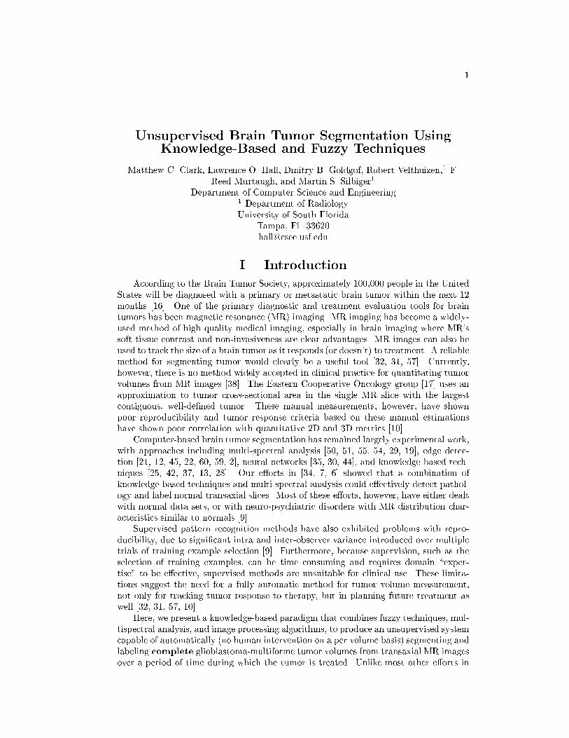
According to the Brain Tumor Society, approximately 100,000 people in the UnitedStates will be diagnosed with a primary or metastatic brain tumor within the next 12months [16]. One of the primary diagnostic and treatment evaluation tools for braintumors has been magnetic resonance (MR) imaging. MR imaging has become a widely-used method of high quality medical imaging, especially in brain imaging where MR'ssoft tissue contrast and non-invasiveness are clear advantages. MR images can also beused to track the size of a brain tumor as it responds (or doesn't) to treatment. A reliablemethod for segmenting tumor would clearly be a useful tool [32, 31, 57]. Currently,however, there is no method widely accepted in clinical practice for quantitating tumorvolumes from MR images [38]. The Eastern Cooperative Oncology group [17] uses anapproximation to tumor cross-sectional area in the single MR slice with the largestcontiguous, well-de�ned tumor. These manual measurements, however, have shownpoor reproducibility and tumor response criteria based on these manual estimationshave shown poor correlation with quantitative 2D and 3D metrics [10].

Computer-based brain tumor segmentation has remained largely experimental work,with approaches including multi-spectral analysis [50, 51, 55, 54, 29, 19], edge detec-tion [21, 12, 45, 22, 60, 59, 2], neural networks [35, 30, 44], and knowledge-based tech-niques [25, 42, 37, 13, 28]. Our e�orts in [34, 7, 6] showed that a combination ofknowledge-based techniques and multi-spectral analysis could e�ectively detect pathol-ogy and label normal transaxial slices. Most of these e�orts, however, have either dealtwith normal data sets, or with neuro-psychiatric disorders with MR distribution char-acteristics similar to normals [9].

Supervised pattern recognition methods have also exhibited problems with repro-ducibility, due to signi�cant intra and inter-observer variance introduced over multipletrials of training example selection [9]. Furthermore, because supervision, such as theselection of training examples, can be time consuming and requires domain \exper-tise" to be e�ective, supervised methods are unsuitable for clinical use. These limita-tions suggest the need for a fully automatic method for tumor volume measurement,not only for tracking tumor response to therapy, but in planning future treatment aswell [32, 31, 57, 10].

Here, we present a knowledge-based paradigm that combines fuzzy techniques, mul-tispectral analysis, and image processing algorithms, to produce an unsupervised systemcapable of automatically (no human intervention on a per volume basis) segmenting andlabeling complete glioblastoma-multiforme tumor volumes from transaxial MR imagesover a period of time during which the tumor is treated. Unlike most other e�orts in

2

segmenting brain pathology, this system has also been tested on a large number of un-seen images with a �xed parameter (rule) set (built from a set of \training images") andquantitatively compared with \ground truth" images. This allows tumor response totherapy to be tracked over repeat scans and aid radiologists in planning subsequenttreatment. More importantly, the system's unsupervised nature avoids the problems ofobserver variability found in supervised methods, providing complete reproducibility ofresults. Furthermore, observer-based training examples are not required, making thesystem suitable for clinical use.

Using knowledge gained during \pre-processing" (pathology detection) in [6, 8],extra-cranial tissues (air, skin, fat, etc.) are �rst removed based on the segmentationcreated by a fuzzy c-means clustering algorithm [5, 23]. The remaining pixels (reallyvoxels since they have thickness) form an intra-cranial mask. An expert system usesinformation from multi-spectral and local statistical analysis to �rst separate suspectedtumor from the rest of the intra-cranial mask, then re�ne the segmentation into a �nalset of regions containing tumor. A rule-based expert system shell, CLIPS [46, 20], isused to organize the system. Low level modules for image processing and high levelmodules for image analysis are all written in C and called as actions from the righthand sides of the rules.

Each slice was classi�ed as abnormal by systems described in [6, 8]. Of the tu-mor types that are found in the brain, glioblastoma-multiformes (Grade IV Gliomas)are the focus of this work. This tumor type was addressed �rst because of its rela-tive compactness and tendency to enhance well with paramagnetic substances, such asgadolinium. For the purposes of tumor volume tracking, segmentations from contigu-ous slices (within the same volume) are merged to calculate total tumor size in 3D. Thetumor segmentation matches well with radiologist-veri�ed \ground truth" images andis comparable to results generated by a supervised segmentation technique.

The remainder of the paper is divided into four sections. Section II. discusses theslices processed and gives a brief overview of the system. Section III. details the system'sthe major processing stages and the knowledge used at each stage. The last two sectionspresent the experimental results, an analysis of them, and future directions for this work.

II. Domain Background

A. Slices of Interest for the Study

The system described here can process any transaxial slice [43, 47] intersecting thebrain cerebrum, starting from an initial slice 7 to 8 cm from the top of the brain andmoving up towards the top of the head and down towards the shoulders. This \initialslice," which simply needs to intersect the ventricles, is used as the starting point dueto the relatively good signal uniformity within the MR coil used [6]. Each brain sliceconsists of three feature images: T1-weighted (T1), proton density weighted (PD), andT2-weighted (T2) [57] .

An example of a normal slice after processing is shown in Figures 1.1(a) and (b).Figures 1.1(c) and (d) show an abnormal slice through the ventricles, though pathologymay exist within any given slice. The labeled normal intra-cranial tissues of interest are:CSF (dark gray) and the parenchymal tissues, white matter (white) and gray matter(black). In the abnormal slice, pathology (light gray) occupies an area that wouldotherwise belong to normal tissues. In the approach described here, only part of thepathology (gadolinium-enhanced tumor) is identi�ed and labeled.

A total of 385 slices containing radiologist diagnosed glioblastoma-multiforme tumorwere available for processing. Table 1..4 in Section IV. lists the distribution of these slices

3

(a)

Ventricles

(b)

(c)

Pathology

(d)

Figure 1.1: Slices of Interest: (a) raw data from a normal slice (T1-weighted, PDand T2-weighted images from left to right) (b) after segmentation (c) raw data froman abnormal slice (T1-weighted, PD and T2-weighted images from left to right) (d)after segmentation. White=white matter; Black=gray matter; Dark Gray=CSF; LightGray=Pathology in (b) and (d).

across 33 volumes of eight patients who received varying levels of treatment, includingsurgery, radiation therapy, and chemo-therapy prior to initial acquisition and betweensubsequent acquisitions. Using a criteria of tumor size (per slice) and level of gadoliniumenhancement to capture the required characteristics of all data sets acquired with thisprotocol, a training subset of 65 slices was created. The heuristics to be discussed inSection III. were manually extracted from the training subset through the process of\knowledge engineering" and are expressed in general terms, such as \higher end of theT1 spectrum" (which does not specify an actual T1 value). This provides knowledgethat is more robust across slices, and avoids dependence on a slice's particular thickness,scanning protocol, or signal intensity, as was the case in [6].

B. Basic MR Contrast Principles

One of the key advantages in MR imaging is its ability to acquire multispectral databy rescanning a patient with di�erent combinations of pulse sequence parameters (in ourcase repetition time (TR), echo time (TE)). For example, the MR data used in this studyconsists of T1, PD, and T2-weighted feature images. A T1-weighted image is producedby a relatively short TR/short TE sequence, a PD-weighted image uses a long TR/shortTE sequence, while a long TR/long TE sequence produces a T2-weighted image [36, 15].For the purpose of brevity, the T1-weighted, PD-weighted, and T2-weighted featureswill be referred to as T1, PD, and T2 respectively.

A particular pulse sequence parameter will provide the best contrast between dif-ferent tissue types [36] and a series of these images can be combined to provide amultispectral data set. The physics of these pulse sequences are outside the scope ofthis paper and their discussion is left to other literature sources [36, 15, 48]. We areprimarily concerned with which pulse sequences best delineate speci�c tissues. Afterreviewing the available literature, a brief synopsis is shown in Table 1..1. This synopsis

4

Table 1..1: A Synopsis of T1, PD, and T2 E�ects on the Magnetic Resonance Image.TR=Repetition Time; TE=Echo Time.

Pulse Sequence E�ect Tissues(TR/TE) (Signal Intensity)

T1-weighted Short T1 relaxation Fat, Proteinaceous Fluid,

(short/short) (bright) Paramagnetic Substances (Gadolinium)

Long T1 relaxation Neoplasms, Edema, CSF,

(dark) Pure Fluid, In ammation

PD-weighted High proton density Fat, Blood

(long/short) (bright) Fluids, CSF

Low proton density Calcium, Air,

(dark) Fibrous Tissue, Cortical Bone

T2-weighted Short T2 relaxation Iron containing substances

(long/long) (dark) (blood-breakdown products)

Long T2 relaxation Neoplasms, Edema, CSF,

(bright) Pure Fluid, In ammation

is the starting point for acquired knowledge, which was re�ned for the speci�c task oftumor segmentation.

C. Knowledge-Based Systems

Knowledge is any chunk of information that e�ectively discriminates one class typefrom another [20]. In this case, tumor will have certain properties that other braintissues will not and visa-versa. In the domain of MRI volumes, there are two primarysources of knowledge available. The �rst is pixel intensity in feature space, whichdescribes tissue characteristics within the MR imaging system (based on a review ofliterature [36, 15, 48]). The second is image/anatomical space and includes expectedshapes and placements of certain tissues within the MR image. As each processing stageis described in Section III., the speci�c knowledge extracted and its application will bedetailed.

D. System Overview

A strength of the knowledge-based (KB) systems in [34, 7, 6] has been their \coarse-to-�ne" operation. Instead of attempting to achieve their task in one step, incrementalre�nement is applied with easily identi�able tissues located and labeled �rst, allowinga \focus" to be placed on the remaining pixels. To better illustrate the system's or-ganization, we present it at a conceptual level. Figure 1.2 shows the primary steps inextracting tumor from raw MR data. Section III. describes these steps in more detail.

The system has �ve primary steps. First a pre-processing stage developed in previ-ous works [34, 7, 6, 8], called Stage Zero here, is used to detect deviations from expectedproperties within the slice. Slices that are free of abnormalities are not processed fur-ther. Otherwise, Stage One extracts the intra-cranial region from the rest of the MRimage based on information provided by pre-processing. This creates an image maskof the brain that limits processing in Stage Two to only those pixels contained by themask.

An initial tumor segmentation is produced in Stage Two through a combinationof adaptive histogram thresholds in the T1 and PD feature images. Additional non-tumor pixels are removed in Stage Three via a \density screening" operation. Density

5

Raw MR image data: T1, PD, and T2-weighted images.

Radiologist’s handlabeled ground truth tumor.

Tumor segmentation refined using ‘‘density screening.’’

STAGE THREE

Initial tumor segmentation using adaptive histogram thresholds on intracranial mask.

STAGE TWO

Intracranial mask created from initial segmentationto reclaim possible losttumor pixels.

STAGE ONE STAGE 0 Pathology Detection.

Slice tissues are located and tested. Slices with detected abnormalities (such as in the white matter class shown) are segmented for tumor. Slices without abnormalities are not processed further.

Initial segmentationby unsupervisedclustering algorithm.

White matter class.

Removal of ‘‘spatial’’ regions that do not contain tumor.

STAGE FOUR

Final thresholding in T1spectrum. Remaining pixels are labeled tumor and processing halts.

STAGE FIVE

Figure 1.2: System Overview.

6

(a) (b) (c) (d) (e)

Figure 1.3: Building the Intra-Cranial Mask. (a) The original FCM-segmented image;(b) pathology captured in Group 1 clusters; (c) intra-cranial mask using only Group 2clusters; (d) mask after including Group 1 clusters with tumor; (e) mask after extra-cranial regions are removed.

screening is based on the observation that pixels of normal tissues are grouped moreclosely together in feature space than tumor pixels.

Stage Four continues tumor segmentation by separately analyzing each spatiallydisjoint \region" in image space created by a connected components operation. Thoseregions found to contain no tumor are removed and the remaining regions are passedto Stage Five for application of a �nal threshold in the T1 spectrum, using the approx-imated tumor boundary (determined with a fuzzy edge detector). The resulting imageis considered the �nal tumor segmentation and can be compared with a ground truthimage.

III. Classi�cation Stages

By its nature, tumor is much more di�cult to model in comparison to normalbrain tissues. Therefore, tumor is de�ned here more by what it isn't than what it is.Speci�cally, the tumor segmentation system operates by removing all pixels considerednot to be enhancing tumor, with all remaining pixels labeled as tumor.

A. Stage Zero: Pathology Detection

All slices processed by the tumor segmentation system have been automaticallyclassi�ed as abnormal. They are known to contain glioblastoma-multiforme tumor basedon radiologist pathology reports. Since this work is an extension of previous work,knowledge generated during \pre-processing" is available to the tumor segmentationsystem. Detailed information can be found in [34, 7, 6, 8], but a brief summary isprovided.

Slice processing begins by using an unsupervised fuzzy c-means (FCM) clusteringalgorithm [5, 23] to segment the slice. The initial FCM segmentation is passed to anexpert system which uses a combination of knowledge concerning cluster distribution infeature space and anatomical information to classify the slice as normal or abnormal.Knowledge implemented in the predecessor system includes rules such as: (1) in a normalslice, CSF belongs to the cluster center with the highest T2 value in the intra-cranialregion; (2) in image space, all normal tissues are roughly symmetrical along the verticalaxis (de�ned by each tissue having approximately the same number of pixels in eachbrain hemisphere). Abnormal slices are detected by their deviation from \expectations"concerning normal MR slices, such as the one shown in Figure 1.2 whose white matterclass failed to completely enclose the ventricle area. An abnormal slice, along withthe facts generated in labeling it abnormal, are passed on to the tumor segmentationsystem. Normal slices have all pixels labeled.

7

(a) (b) (c)

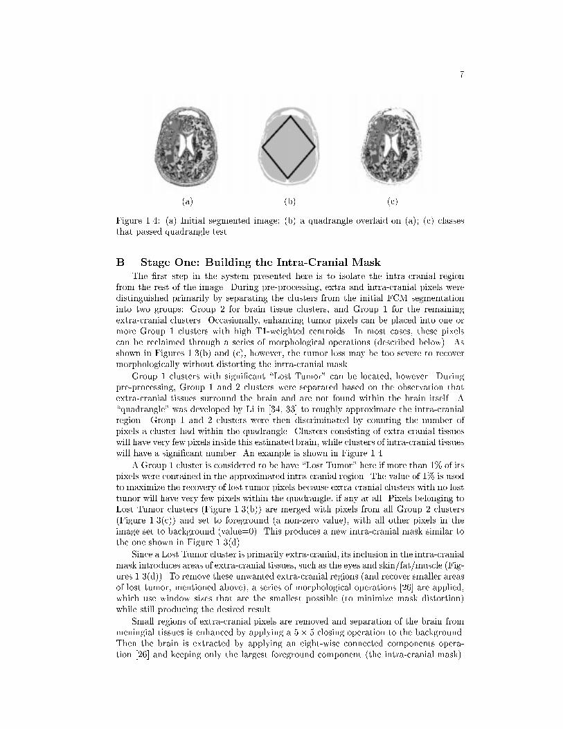
Figure 1.4: (a) Initial segmented image; (b) a quadrangle overlaid on (a); (c) classesthat passed quadrangle test.

B. Stage One: Building the Intra-Cranial Mask

The �rst step in the system presented here is to isolate the intra-cranial regionfrom the rest of the image. During pre-processing, extra and intra-cranial pixels weredistinguished primarily by separating the clusters from the initial FCM segmentationinto two groups: Group 2 for brain tissue clusters, and Group 1 for the remainingextra-cranial clusters. Occasionally, enhancing tumor pixels can be placed into one ormore Group 1 clusters with high T1-weighted centroids. In most cases, these pixelscan be reclaimed through a series of morphological operations (described below). Asshown in Figures 1.3(b) and (c), however, the tumor loss may be too severe to recovermorphologically without distorting the intra-cranial mask.

Group 1 clusters with signi�cant \Lost Tumor" can be located, however. Duringpre-processing, Group 1 and 2 clusters were separated based on the observation thatextra-cranial tissues surround the brain and are not found within the brain itself. A\quadrangle" was developed by Li in [34, 33] to roughly approximate the intra-cranialregion. Group 1 and 2 clusters were then discriminated by counting the number ofpixels a cluster had within the quadrangle. Clusters consisting of extra-cranial tissueswill have very few pixels inside this estimated brain, while clusters of intra-cranial tissueswill have a signi�cant number. An example is shown in Figure 1.4.

A Group 1 cluster is considered to be have \Lost Tumor" here if more than 1% of itspixels were contained in the approximated intra-cranial region. The value of 1% is usedto maximize the recovery of lost tumor pixels because extra-cranial clusters with no losttumor will have very few pixels within the quadrangle, if any at all. Pixels belonging toLost Tumor clusters (Figure 1.3(b)) are merged with pixels from all Group 2 clusters(Figure 1.3(c)) and set to foreground (a non-zero value), with all other pixels in theimage set to background (value=0). This produces a new intra-cranial mask similar tothe one shown in Figure 1.3(d).

Since a Lost Tumor cluster is primarily extra-cranial, its inclusion in the intra-cranialmask introduces areas of extra-cranial tissues, such as the eyes and skin/fat/muscle (Fig-ures 1.3(d)). To remove these unwanted extra-cranial regions (and recover smaller areasof lost tumor, mentioned above), a series of morphological operations [26] are applied,which use window sizes that are the smallest possible (to minimize mask distortion)while still producing the desired result.

Small regions of extra-cranial pixels are removed and separation of the brain frommeningial tissues is enhanced by applying a 5� 5 closing operation to the background.Then the brain is extracted by applying an eight-wise connected components opera-tion [26] and keeping only the largest foreground component (the intra-cranial mask).

8

(a)

T1-Weighted Value

PD

-Wei

gh

ted

Val

ue

CPa

Pa

Pa

T

T

T

High PD

High T1

(b)

Figure 1.5: (a) Raw T1, PD, and T2-weighted Data. The distribution of intra-cranialpixels are shown in (b) T1-PD feature space. C = CSF, Pa = Parenchymal Tissues, T= Tumor

Finally, \gaps" along the periphery of the intra-cranial mask are �lled by �rst applyinga 15� 15 closing, then a 3� 3 erosion operation. An example of the �nal intra-cranialmask can be seen in Figure 1.3(e).

C. Stage Two: Multi-spectral Histogram ThresholdingGiven an intra-cranial mask, there are three primary tissue types: pathology (which

can include gadolinium-enhanced tumor, edema, and necrosis), the brain parenchyma(white and gray matter), and CSF. We would like to remove as many pixels belongingto normal tissues as possible from the mask.

Each MR voxel of interest has a hT1; PD; T2i location in <3, forming a feature-space distribution. Based on the fact that pixels belonging to the same tissue type willexhibit similar relaxation behaviors (T1 and T2) and water content (PD), they will thenalso have approximately the same location in feature space [3]. Figure 1.5(a) shows thesignal-intensity images of a typical slice, while (b) shows a histogram for the bivariatefeatures T1/PD with approximate tissue labels overlaid. There is some overlap betweenclasses because the graphs are projections and also due to \partial-averaging" wheredi�erent tissue types are quantized into the same pixel/voxel.

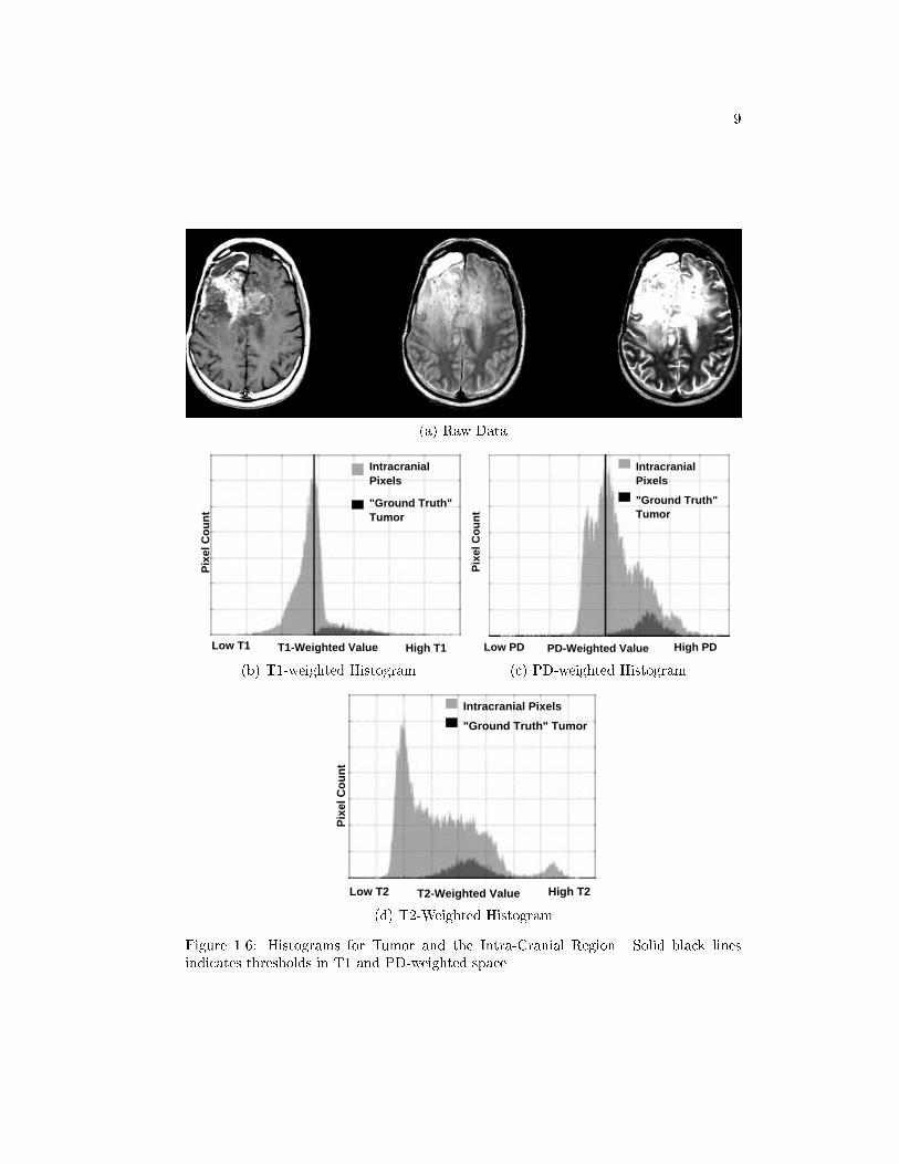
The typical relationships between enhancing tumor and other brain tissues can alsobe seen in Figure 1.6, which are histograms for each of the three feature images. Thesedistributions were examined and interviews were conducted with experts concerning thegeneral makeup of tumorous tissue, and the behavior of gadolinium enhancement in thethree MRI protocols. From these sources, a set of heuristics were extracted that couldbe included in the system's knowledge base:

1. Gadolinium-enhanced tumor pixels occupy the higher end of the T1 spectrum.

2. Gadolinium-enhanced tumor pixels occupy the higher end of the PD spectrum,though not with the degree of separation found in T1 space [24].

3. Gadolinium-enhanced tumor pixels were generally found in the \middle" of theT2 spectrum, making segmentation based on T2 values di�cult.

4. Slices with greater enhancement had better separation between tumor and non-tumor pixels, while less enhancement resulted in more overlap between tissuetypes.

Analysis of these heuristics revealed that histogram thresholding could provide asimple, yet e�ective, mechanism for gross separation of tumor from non-tumor pixels(and thereby an implementation for the heuristics). In fact, in the T1 and PD spectrums,

9

(a) Raw Data

T1-Weighted Value High T1Low T1

Pix

el C

ou

nt

Intracranial Pixels

"Ground Truth" Tumor

(b) T1-weighted Histogram

PD-Weighted Value High PDLow PD

Pix

el C

ou

nt

Intracranial Pixels

"Ground Truth" Tumor

(c) PD-weighted Histogram

T2-Weighted Value High T2Low T2

Pix

el C

ou

nt

Intracranial Pixels

"Ground Truth" Tumor

(d) T2-Weighted Histogram

Figure 1.6: Histograms for Tumor and the Intra-Cranial Region. Solid black linesindicates thresholds in T1 and PD-weighted space.

10

(a) (b) (c) (d)

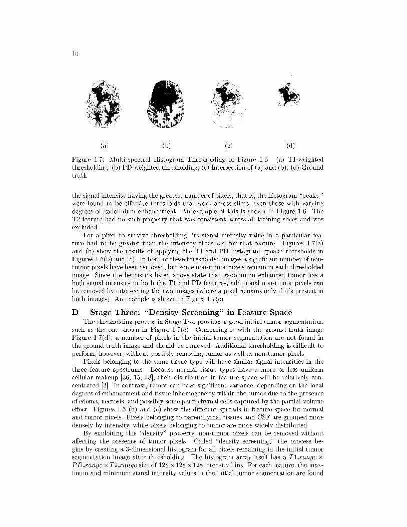
Figure 1.7: Multi-spectral Histogram Thresholding of Figure 1.6. (a) T1-weightedthresholding; (b) PD-weighted thresholding; (c) Intersection of (a) and (b); (d) Groundtruth.

the signal intensity having the greatest number of pixels, that is, the histogram \peaks,"were found to be e�ective thresholds that work across slices, even those with varyingdegrees of gadolinium enhancement. An example of this is shown in Figure 1.6. TheT2 feature had no such property that was consistent across all training slices and wasexcluded.

For a pixel to survive thresholding, its signal intensity value in a particular fea-ture had to be greater than the intensity threshold for that feature. Figures 1.7(a)and (b) show the results of applying the T1 and PD histogram \peak" thresholds inFigures 1.6(b) and (c). In both of these thresholded images a signi�cant number of non-tumor pixels have been removed, but some non-tumor pixels remain in each thresholdedimage. Since the heuristics listed above state that gadolinium enhanced tumor has ahigh signal intensity in both the T1 and PD features, additional non-tumor pixels canbe removed by intersecting the two images (where a pixel remains only if it's present inboth images). An example is shown in Figure 1.7(c).

D. Stage Three: \Density Screening" in Feature SpaceThe thresholding process in Stage Two provides a good initial tumor segmentation,

such as the one shown in Figure 1.7(c). Comparing it with the ground truth imageFigure 1.7(d), a number of pixels in the initial tumor segmentation are not found inthe ground truth image and should be removed. Additional thresholding is di�cult toperform, however, without possibly removing tumor as well as non-tumor pixels.

Pixels belonging to the same tissue type will have similar signal intensities in thethree feature spectrums. Because normal tissue types have a more or less uniformcellular makeup [36, 15, 48], their distribution in feature space will be relatively con-centrated [3]. In contrast, tumor can have signi�cant variance, depending on the localdegrees of enhancement and tissue inhomogeneity within the tumor due to the presenceof edema, necrosis, and possibly some parenchymal cells captured by the partial-volumee�ect. Figures 1.5 (b) and (c) show the di�erent spreads in feature space for normaland tumor pixels. Pixels belonging to parenchymal tissues and CSF are grouped moredensely by intensity, while pixels belonging to tumor are more widely distributed.

By exploiting this \density" property, non-tumor pixels can be removed withouta�ecting the presence of tumor pixels. Called \density screening," the process be-gins by creating a 3-dimensional histogram for all pixels remaining in the initial tumorsegmentation image after thresholding. The histogram array itself has a T1 range �PD range�T2 range size of 128�128�128 intensity bins. For each feature, the max-imum and minimum signal intensity values in the initial tumor segmentation are found

11

Low PD

HighPDLow

T1 High T1

Num

ber

of P

ixel

s

Low

High

(a) 2D-Histogram Projection

Lo

w P

D

Low T1 High T1

Hig

h P

D

(b) ScatterplotBefore Screening

Low T1 High T1

Lo

w P

DH

igh

PD

(c) ScatterplotAfter Screening

(d) Initial Tumor (e) Removed Pixels (Black) (f) Ground Truth

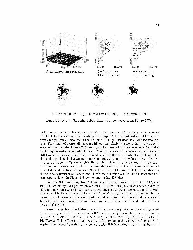
Figure 1.8: Density Screening Initial Tumor Segmentation From Figure 1.7(c).

and quantized into the histogram array (i.e., the minimum T1 intensity value occupiesT1 Bin 1, the maximum T1 intensity value occupies T1 Bin 128), with all T1 values inbetween \quantized" into one of the 128 bins. This quantization was done for two rea-sons. First, sizes of a three-dimensional histogram quickly became prohibitively large tostore and manipulate. Even a 2563 histogram has nearly 17 million elements. Secondly,levels of quantization can make the \dense" nature of normal pixels more apparent whilestill leaving tumor pixels relatively spread out. For the 12-bit data studied here, afterthresholding, slices had a range of approximately 800 intensity values in each feature.The actual value of 128 was empirically selected. Using 64 bins blurred the separationof tumor and non-tumor pixels in training slices where the tumor boundary was notas well de�ned. Values similar to 128, such as 120 or 140, are unlikely to signi�cantlychange the \quantization" e�ect and should yield similar results. The histograms andscatterplots shown in Figure 1.8 were created using 128 bins.

From the 3D histogram, three 2D projections are generated: T1/PD, T1/T2, andPD/T2. An example 2D projection is shown in Figure 1.8(a), which was generated fromthe slice shown in Figure 1.7(c). A corresponding scatterplot is shown in Figure 1.8(b).The bins with the most pixels (the highest \peaks" in Figure 1.8(a)) can be seen in thelowest T1/PD corner and are comprised of non-tumorous pixels that should be removed.In contrast, tumor pixels, while greater in number, are more widespread and have lowerpeaks in their bins.

In each projection, the highest peak is found and designated as the starting pointfor a region growing [27] process that will \clear" any neighboring bin whose cardinality(number of pixels in that bin) is greater than a set threshold (T1/PD=3, T1/T2=4,PD/T2=3). This will result in a new scatterplot similar to that shown in Figure 1.8(c).A pixel is removed from the tumor segmentation if it is located in a bin that has been

12

(a) (b) (c)

Figure 1.9: Regions in Image Space. After processing the intra-cranial mask (a), (b) isan initial tumor segmentation. Only one region, as shown in the ground-truth image(c) is actual tumor. Region analysis discriminates between tumorous and non-tumorousregions.

\cleared" in any of the three feature-domain projections. Figures 1.8(d) and (e) are thetumor segmentation before and after the entire density screening process is completed.Note that the resulting image is closer to ground truth.

The thresholds used were determined from training slices by creating a 3D his-togram, including 2D projections, using only pixels contained in the initial tumor seg-mentation. Then the ground truth tumor pixels for each slice were overlaid on therespective projections. So, given a 3D histogram of an initial tumor segmentation, allpixels not in the ground truth image are removed, leaving only tumor behind withoutchanging the dimensions and quantization levels of the histogram. The respective 2Dprojections of all training slices were examined. It was found that the smallest bin cardi-nality bordering a bin occupied by known non-tumor pixels made an accurate thresholdfor the given projection.

E. Stage Four: Region Analysis and LabelingIn Stages Two and Three, the knowledge extracted up to this point was applied to

pixels individually. Stage Four, allows spatial information to be introduced by consider-ing pixels on a region or component level. Applying an eight-wise connected componentsoperation [26] to the re�ned tumor segmentation generated by Stage Three, allows eachregion to be tested separately for the presence of tumor. An example is shown in Fig-ure 1.9. After processing the intra-cranial mask shown in Figure 1.9(a) in Stages Twoand Three, a re�ned tumor segmentation (b) is produced. The segmentation shows anumber of spatially disjoint areas, but ground truth tumor in Figure 1.9(c) shows thatonly one region actually contains tumor. Therefore, decisions must be made regardingwhich regions contain tumor and which do not.

1. Removing Meningial Regions

In addition to tumor, meningial tissues immediately surrounding the brain, suchas the dura or pia mater, receive gadolinium infused blood. As a result they can havea high T1 signal intensity that may violate with the knowledge base's assumption inSection 2. that regions with the highest T1 value are most likely tumor. These extra-cranial tissues can be identi�ed and removed via anatomical knowledge by noting thatsince they are thin membranes, meningial regions should lie along the periphery of thebrain in a relatively narrow margin.

Figure 1.10 shows that an approximation of the brain periphery can be used todetect meningial tissues. The unusual shape of the intra-cranial region is due to prior

13

(a) (b) (c) (d) (e)

Figure 1.10: Removing Meningial Pixels. A \ring" that approximates the brain pe-riphery is created by applying a 7� 7 erosion operation to the intra-cranial mask (a),resulting in image (b). Subtracting (b) from (a), creates a \ring", shown in (c). Byoverlaying this \ring" onto a tumor segmentation (d), small regions of meningial tissues(e) can be detected and removed. The unusual shape of the intra-cranial region is dueto prior resection surgery.

resection surgery. The periphery is created by applying a 7 � 7 erosion operation tothe intra-cranial mask and subtracting the resultant image from the original mask, asshown in Figure 1.10(a-c). Each component or separate region in the re�ned tumormask is now intersected with the brain periphery. Any region which has more than50% of its pixels contained in the periphery is marked as meningial tissue and removed.Figure 1.10(d) shows a tumor segmentation which is intersected with the periphery fromFigure 1.10(c). In Figure 1.10(e), the pixels that will be removed by this operation areshown and they are indeed meningial pixels.

2. Removing Non-Tumor Regions

Once any extra-cranial regions have been removed, the knowledge base is applied todiscriminate between regions with and without tumor based on statistical informationabout the region. A region mean, standard deviation, and skewness in hT1i, hPDi,and hT2i feature space respectively are used as features. The concept exploited is thattrends and characteristics described at a pixel level in Section C. are also applicable ona region level. By sorting regions in feature space based upon their mean values, rulesbased on their relative order can be created:

1. Large regions that contain tumor will likely contain a signi�cant number of pixelsthat are of highest intensity in T1 and PD space, while regions without tumorlikely contain a signi�cant number of pixels of lowest intensity in T1 and PDspace.

2. The means of regions with similar tissue types neighbor one another in featurespace.

3. The intra-cranial region with the highest mean T1 value and a \high" PD and T2value, is considered \First Tumor," against which all other regions are compared.

4. Other regions that contain tumor are likely to fall within 1 to 1.5 standard devi-ations (depending on region size) of First Tumor in T1 and PD space.

While most glioblastoma-multiforme tumor cases have only one tumorous spatiallycompact region that has the highest mean T1 value, in some cases, the tumor hasgrown such that it has branched into both hemispheres of the brain, causing the tumorto appear disjoint in some slices, or it has fragmented as a result of treatment. Also,

14

(a) (b) (c) (d) (e)

Figure 1.11: Using Pixel Counts to Remove Non-Tumorous Regions. Given a re�nedtumor segmentation after Stage Three (a), spatial regions with a signi�cant number ofpixels highest in T1 space (b) or PD space (c) are likely to contain tumor. Regions withpixels lowest in T1 space (d) are unlikely to contain signi�cant tumor. Ground truth isshown in (e).

Table 1..2: Region Labeling Rules Based on Pixel Presence.Region Size Pixels in intersections with the 3 masks Action

� 5 Any Bottom T1 Pixels AND RemoveLess than 2 Top T1 Pixels Non-Tumor

� 500 More than RegionSize� 0:06 Top T1 Pixels Label AsTumor

� 5 No Top T1 Pixels AND RemoveMore Than RegionSize� 0:005 Bottom T1 Pixels AND

Less Than RegionSize� 0:01 Top PD Pixels

di�erent tumor regions do not enhance equally. Thus, cases can range from a singlewell-enhancing tumor to a fragmented tumor with di�erent levels of enhancement. Incomparison, the makeup of non-tumor regions is generally more consistent than intumorous regions. Therefore, the knowledge base is designed to facilitate removal of non-tumor regions because their composition can be more reliably modeled and detected.

Regions that comply with the �rst heuristic listed above are the easiest to locateand their statistics can be used to examine the remaining regions. To apply the �rstheuristic, three new image masks are created. The �rst image mask takes the re�nedtumor segmentation image and keeps only 20% of the highest T1 value pixels (i.e., ifthere were 100 pixels in the re�ned tumor image, the 20 pixels with the highest T1values are kept). The second mask keeps the highest 20% in PD space, while the thirdmask keeps the 30% lowest in T1 space. Each region is isolated and intersected witheach of the 3 masks created. The number of pixels of the region in a particular maskis recorded and compared with the rules listed in Table 1..2. An example is shown inFigure 1.11.

Regions that do not activate any of the rules in Table 1..2 remain unlabeled and areanalyzed using the last two heuristics.

According to the third heuristic, given a region that has been positively labeledtumor as a point of reference, a search can be made in feature space for neighboringtumor regions. Normally, the region with the highest T1 mean value can be selected asthis point of reference (called \First Tumor"). To guard against the possibility that anextra-cranial region (usually meningial tissues at the inter-hemispheric �ssure) has beenselected instead, the selected region is veri�ed via the heuristic that a tumor region willnot only have a very high T1 mean value, but will also occupy the highest half of all

15

Table 1..3: Region Labeling Rules Based on Statistical Measurements. Largest is thelargest known tumor region.

(a) Rules Based on Standard Deviation (SD) of \First Tumor"Region Size If Region's Mean Values are: Action

� 10 OR More than 1 SD away in T1 space OR Remove� Largest=4 More than 1 SD away in PD space.

� 10 AND More than 1.5 SD away in T1 space AND Remove� Largest=4 More than 1.5 SD away in PD space.

(b) Labeling Rules Based on Region Statistics� 100 Region T1 Skewness � 0:75 AND Remove

Region PD Skewness � 0:75 AND

Region T2 Skewness � 0:75

regions in sorted PD and T2 mean space. For example, if there were 10 regions total,the region being tested must be one of the 5 highest mean values in both PD and T2space. If the candidate region passes, it is con�rmed as First Tumor. Otherwise, it isdiscarded and the region with the next highest T1 mean value is selected for testing asFirst Tumor.

Once First Tumor has been con�rmed, the search for neighboring tumor regions canbegin. Although tumorous regions can have between-slice variance, the third and fourthheuristics hold for the purpose of separating tumor from non-tumor regions within agiven slice. Furthermore, the standard deviations in T1 and PD space of a known tumorregion were found to be a useful and exible distance measure.

Table 1..3(a) lists the two rules that used the standard deviation to remove non-tumor regions, based on the size (number of pixels) of the region being tested. The rulein Table 1..3(b) serves as a tie-breaker for some regions that were not labeled before.The term Largest is used to indicate the largest known tumor region. In most casesthere was only a single tumor region, so the \�rst tumor" region was also the Largestregion. In cases where tumor was fragmented, however, a larger tumorous region wouldhave a greater number of pixels (and thus, more reliable sample) to calculate the meanand standard deviation for the distance measure. Therefore, the system would �ndLargest by searching for the largest region that was within one standard deviation inboth T1 and PD space to the First Tumor region. After the rules in Table 1..3 areapplied, all regions that were not removed are kept as regions containing tumor.

F. Stage Five: Final T1 ThresholdAt the end of Stage Four, the regions with no tumor have been removed, but non-

tumor pixels may still be found in those regions considered to contain tumor. Whileenhancing tumor has properties in each of the three available features that have beenused as knowledge, discussions with an expert radiologist [39] have indicated that �naltumor boundaries are determined by pixel intensities in the T1-weighted image. Thresh-olds were described in Section C. in a relatively coarse manner because the boundaryof enhancing tumor was \obscured" by pixels belonging to non-tumor tissues. Withthe removal of most of these non-tumor tissues in Stages Two through Four, however,a greater level of focus can be placed and a more precise threshold can be applied.

The threshold is determined using the principle that the spatial boundary betweenenhancing tumor and surrounding tissues contain pixels whose signal intensities cor-respond to the tumor/non-tumor boundary in T1-weighted space. One of the mostcommon methods of isolating spatial boundaries between objects of interest (with dif-

16

ferent intensities) has been edge detection. In our case, edges represent di�erences inT1-weighted signal intensities, the more distinct boundary a tumor has, the greater itsedge strength will be.

Most edge-detection based methods, such as those in [21, 12, 45, 22, 60, 59, 2] at-tempt to use edges to trace the tumor's contours. This can work well for tumors withdistinct boundaries, as shown in Figure 1.12(d) using a standard Sobel operator, but canhave signi�cant problems with more di�use tumors, shown in Figure 1.12(i). A varietyof edge detection operators have been introduced, such as Canny and Bergholm [27].Most of these, however, have a number of parameters that are di�cult to automaticallyoptimize, especially in a domain where the object of interest can have such wide rang-ing characteristics [14]. As a result, Dellepiane [12] and Ra� and Newman [45] havesuggested that edge detection is unlikely to work reliably for complex structures liketumors.

Edge detection may still provide knowledge to be exploited, however. By notingthat edges not only approximate the tumor boundary spatially, but can also indicatethe approximate signal intensity of that boundary which can be used in a thresholdoperation. Now detected edges need not be perfect, merely su�cient to indicate theappropriate signal intensity. Edge detection must still be reasonable, however, for themethod to work.

To address the problem of detecting edges in tumors with di�use, and to minimizethe problem of parameter optimization, the technique introduced here uses a \fuzzy"approach to edge detection presented by Tao and Thompson in [49] which used fuzzyif-then rules that were based on the relationship between each pixel and its eight-wiseneighbors. Structure elements, sixteen in total with examples shown in Figure 1.13, areused to develop a fuzzy if-then rule:IF [the di�erences (Dx's) between the intensities of the pixels (marked with \x") and thecenter pixel are small] AND [the di�erences (D's) between the intensities of the pixels(not marked with \x") and the center pixel are large] THEN the center pixel of thisstructure is an edge pixel.

The authors state that the fuzzy memberships small and large are de�ned with abell-shaped function, though they do not specify a particular function. Here, a Gaussian-based function is used and the fuzzy set small is de�ned as:

�small = e�Diff2

(a;b)

2�2

where Diff(a;b) is the absolute intensity di�erence between the center pixel and theeight-wise neighbor (a,b). The fuzzy set large is de�ned as: �large = 1��small. The ac-tual Gaussian formula is not used to allow a membership of �small = 1:0 to be returnedwhen Diff = 0. Also, in a standard Gaussian function, the value � represents the stan-dard deviation. For de�ning the fuzzy set, it controls how quickly �small decreases (and�large increases) as the intensity di�erence, Diff , becomes larger. In this preliminarystudy, � = 2:0, though it could be possible to have rules in the knowledge-base adjustthe value according to a tumor's characteristics.

The fuzzy if-then rule described above is used to determine a pixel's \edge potential"(PEP) within a given edge structure (Figure 1.13) by calculating the membershipsbetween the center pixel and each of it eight-wise neighbors for the fuzzy set small(if the neighbor is covered by an \x" in the edge structure) or large (if the neighboris uncovered), and returning the minimum membership. For example, using the �rststructure (PEP1) in Figure 1.13, its edge potential would be:�PEP1(x; y) = min(�small(Diff(x�1;y�1)); �small(Diff(x�1;y�1)); �small(Diff(x�1;y));

�small(Diff(x�1;y+1)); �small(Diff(x;y�1)); �small(Diff(x;y+1));

17

(a) Raw Data

(b) GT Tumor (c) KB Tumor (d) Sobel Edge (e) Fuzzy Edge

(f) Raw Data

(g) GT Tumor (h) KB Tumor (i) Sobel Edges (j) Fuzzy Edges

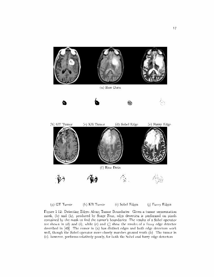
Figure 1.12: Detecting Edges Along Tumor Boundaries. Given a tumor segmentationmask, (b) and (h), produced by Stage Four, edge detection is performed on pixelscontained by the mask to �nd the tumor's boundaries. The results of a Sobel operatorare shown in (d) and (i), while (e) and (j) show the results of a fuzzy edge detectordescribed in [49]. The tumor in (a) has distinct edges and both edge detectors workwell, though the Sobel operator more closely matches ground truth (b). The tumor in(e), however, performs relatively poorly, for both the Sobel and fuzzy edge detectors.

18

X

XX

X

XX

X

XX X

XX

X

XXXX

X

X

X

XX

X X

Figure 1.13: Edge Structures for Fuzzy Edge Detection. Edge structures, examplesshown above, are used to generate the fuzzy if-then rules. Neighboring pixels coveredby an \x" are used to calculate membership in the fuzzy set small, while those uncoveredare used to calculate membership in the fuzzy set large.

�large(Diff(x+1;y�1)); �large(Diff(x+1;y)); �large(Diff(x+1;y+1)))

Given sixteen edge structures, a pixel will have sixteen possible edge memberships.The pixel's �nal edge membership is set by keeping the membership of the structurethe best matched the edge (i.e., the structure with the highest membership). Formally:

PEP (x; y) = max(�PEP1(x; y); : : : ; �PEP16(x; y))

Once �nal edge memberships have been calculated for all pixels, the detected edgesare \thinned" by removing redundant edge pixels through a local maxima operation.A \pseudo-centroid" of the remaining edge strengths is then calculated and only thoseedges that are stronger than the pseudo-centroid are kept, producing a �nal edge image,similar to those shown in Figures 1.12(f) and (j).

The method proposed by Tao and Thompson was implemented as described in [49]with the addition that the technique only considers pixels contained in an image mask(in this case, the tumor segmentation mask produced at the end of Stage Four). Oncethe �nal edge image is produced, the �nal T1 threshold is calculated by averaging theT1 signal intensities of all pixels contained in the �nal edge image. During averaging,the signal intensities are not weighted by edge strength as it did not signi�cantly a�ectthe �nal T1 threshold. Once the T1 threshold is calculated, it is applied to the tumorsegmentation image produced at the end of Stage Four (keeping only those pixels whoseT1 signal intensity is greater than the T1 threshold). The resultant image is consideredthe �nal tumor segmentation and processing halts.

IV. Results

A total of 385 slices from 33 volumes across 8 patients diagnosed with glioblastoma-multiforme tumor, who also underwent radiation and chemo-therapy treatment, wereavailable for processing. From this data set, 65 training slices, shown in Table 1..4, wereextracted and used to construct the knowledge base and rules.

After processing by the system, the knowledge-based tumor segmentations werecompared with radiologist-veri�ed \ground-truth" tumor segmentations [56], as well asthree supervised methods. To measure how well (on a pixel level) a tumor segmentationcompares with ground truth, two metrics were used. The �rst, \Percent Match," issimply the number of true positives divided by the total tumor size. The second, iscalled a \Correspondence Ratio," and was created to account for the presence of falsepositives:

Correspondence Ratio =True Pos. � (0:5 � False Pos.)

Number Pixels in Ground Truth Tumor

19

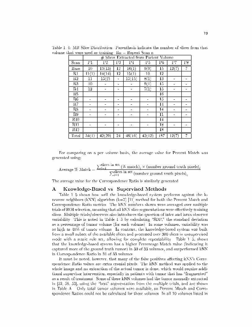
Table 1..4: MR Slice Distribution. Parenthesis indicate the number of slices from thatvolume that were used as training. Rn = Repeat Scan n.

# Slices Extracted from Patient VolumeScan P1 P2 P3 P4 P5 P6 P7 P8

Base 10 13(13) 12 16(1) 9(9) 15 12(7) 7R1 11(1) 14(14) 12 15(1) 10 12R2 11 15(2) - 15(15) 8(1) 13 - -R3 10 - - - 8(1) 15 - -R4 12 - - - 7(1) 15 - -R5 - - - - - 16 - -R6 - - - - - 15 - -R7 - - - - - 14 - -R8 - - - - - 14 - -R9 - - - - - 11 - -R10 - - - - - 14 - -R11 - - - - - 18 - -R12 - - - - - 18 - -

Total 54(1) 42(29) 24 46(16) 42(12) 187 12(7) 7

For comparing on a per volume basis, the average value for Percent Match wasgenerated using:

Average % Match =

Pslices in seti=1 (% match)i � (number ground truth pixels)iPslices in set

i=1 (number ground truth pixels)i

The average value for the Correspondence Ratio is similarly generated.

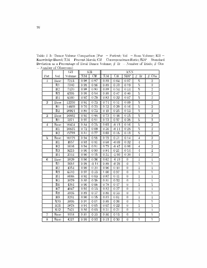
A. Knowledge-Based vs. Supervised MethodsTable 1..5 shows how well the knowledge-based system performs against the k-

nearest neighbors (kNN) algorithm (k=7) [11] method for both the Percent Match andCorrespondence Ratio metrics. The kNN numbers shown were averaged over multipletrials of ROI selection, meaning that all kNN slice segmentations were e�ectively trainingslices. Multiple trials/observers also introduces the question of inter and intra-observervariability. This is noted in Table 1..5 by calculating \SDP," the standard deviationas a percentage of tumor volume (for each volume). In some volumes, variability wasas high as 40% of tumor volume. In contrast, the knowledge-based system was builtfrom a small subset of the available slices and processed over 300 slices in unsupervisedmode with a static rule set, allowing for complete repeatability. Table 1..5, showsthat the knowledge-based system has a higher Percentage Match value (indicating itcaptured more of the ground truth tumor) in 30 of 33 volumes, and outperformed kNNin Correspondence Ratio in 31 of 33 volumes.

It must be noted, however, that many of the false positives a�ecting kNN's Corre-spondence Ratio values are extra-cranial pixels. The kNN method was applied to thewhole image and no extraction of the actual tumor is done, which would require addi-tional supervisor intervention, especially in patients with tumor that has \fragmented"as a result of treatment. Some of these kNN volumes had the tumor manually extractedin [52, 58, 53], using the \best" segmentation from the multiple trials, and are shownin Table A.. Only total tumor volumes were available, so Percent Match and Corre-spondence Ratios could not be calculated for these volumes. In all 10 volumes listed in

20

Table 1..5: Tumor Volume Comparison (Pat. = Patient; Vol. = Scan Volume; KB =Knowledge Based; %M=Percent Match; CR = Correspondence Ratio; SDP = StandardDeviation as a Percentage of Total Tumor Volume; # Tr. = Number of Trials; # Obs.= Number of Observers)

GT KB kNNPat. Vol. Volume %M CR %M CR SDP # Tr. # Obs

1 Base 7213 0.98 0.87 0.89 0.64 0.07 5 2R1 7240 0.98 0.86 0.89 0.52 0.19 5 2R2 7470 0.98 0.80 0.88 0.54 0.14 5 2R3 6395 0.98 0.84 0.88 0.47 0.40 5 2R4 6560 0.97 0.79 0.83 0.32 0.07 5 2

2 Base 12230 0.91 0.73 0.74 0.51 0.09 5 2R1 14609 0.76 0.70 0.52 0.29 0.16 5 2R2 20924 0.80 0.73 0.49 0.25 0.13 5 2

3 Base 10892 0.92 0.88 0.73 0.46 0.15 5 3R1 5971 0.97 0.81 0.72 0.37 0.28 5 3

4 Base 10454 0.84 0.75 0.63 -0.13 0.16 5 2R1 10835 0.72 0.69 0.56 -0.14 0.28 5 2R2 15788 0.81 0.77 0.69 0.15 0.13 5 2

5 Base 10178 0.94 0.88 0.79 0.51 0.14 4 2R1 4657 0.93 0.81 0.68 -0.09 0.32 4 2R2 5616 0.94 0.81 0.79 -0.47 0.06 4 2R3 9215 0.96 0.90 0.84 0.21 0.14 4 2R4 3544 0.90 0.55 0.51 -1.90 0.20 4 2

6 Base 5829 0.96 0.36 0.62 -0.19 0 1 1R1 2684 0.98 -0.14 0.88 -0.38 0 1 1R2 4354 0.99 0.20 0.96 0.40 0 1 1R3 6510 0.97 0.53 1.00 0.97 0 1 1R4 8688 0.92 0.63 0.87 0.41 0 1 1R5 3079 0.80 0.38 0.81 0.32 0 1 1R6 4384 0.96 0.66 0.78 0.47 0 1 1R7 4047 0.92 0.53 0.82 0.27 0 1 1R8 3935 0.89 0.57 0.80 0.53 0 1 1R9 3201 0.90 0.55 0.85 0.61 0 1 1R10 3895 0.91 0.61 0.88 0.26 0 1 1R11 5878 0.94 0.65 0.67 0.22 0 1 1R12 7421 0.86 0.63 0.51 0.21 0 1 1

7 Base 1018 0.81 0.50 0.86 0.13 0 1 1

8 Base 4521 0.99 0.92 0.53 0.30 0 1 1

21

Table 1..6: Knowledge-Based Tumor vs. kNN. (Pat. = Patient; GT = Ground truthvolume; KB = Knowledge-based; kNN SDP = kNN Standard Deviation as Percentageof Tumor Volume; Manual kNN = kNN volume after manual tumor extraction.)

Pat. Scan GT KB kNN kNN ManualVol. Vol. Vol. SDP kNN

1 Base 7213 8561 10022 0.07 6334R1 7240 8829 11958 0.19 6794R2 7470 9928 11576 0.14 6616R3 6395 8132 10870 0.40 5901R4 6560 8614 12115 0.07 5690

5 Base 10178 10784 14044 0.14 7938R1 4657 5489 10279 0.32 2834R2 5616 6773 18603 0.06 3952R3 9215 9833 18210 0.14 6729R4 3544 5730 19138 0.20 3035

Table A., manually extracted kNN consistently underestimated tumor volume, meaningthe method missed more radiologist veri�ed tumor than the knowledge-based method,signi�cantly in some cases.

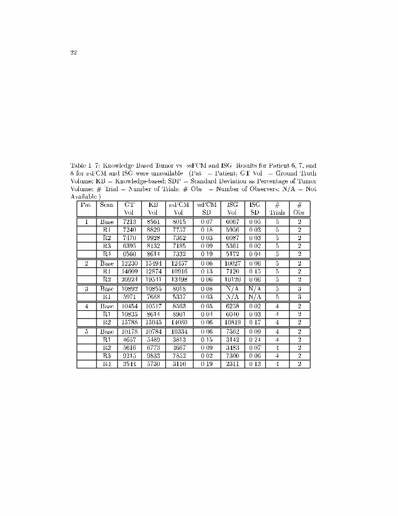
A comparison is also made against the semi-supervised FCM (ssFCM) algorithm,which was initialized with the same ROI's used to initialize kNN in Table 1..5 [52, 58, 53].The resultant ssFCM segmentation was then used to initialize ISG, a commercially avail-able seed-growing tool (ISG Technologies, Toronto, Canada) for supervised evaluationof tumor volumes. The ISG processing also removed any extra-cranial tissues found inthe ssFCM segmentation. Results available for the volumes processed by ssFCM andISG are shown in Table 1..7. The results reported in Table 1..7 are a mean over theset of trials performed for that volume and thus have a standard deviation, also listed.Only �nal tumor volumes were available from [52, 58, 53] ssFCM and ISG.

In terms of absolute di�erence, the ssFCM approach was closer to ground truth thanthe knowledge-based method in 10 out of 18 volumes, with 6 of these cases by more thanthe standard deviation of the ssFCM volume. In the 8 cases where the knowledge-basedmethod gave better results, however, 7 of them were better than ssFCM by more thanthe standard deviation. The knowledge-based method performs better against ISG, in9 out of 16 cases, with all 9 by more than the standard deviation of ISG. Furthermore,ssFCM underestimated total tumor volume in 12 instances, while ISG underestimatedtumor volume in all 16 available volumes, which is not helpful for any use involvingtreatment since the methods missed more radiologist veri�ed tumor.

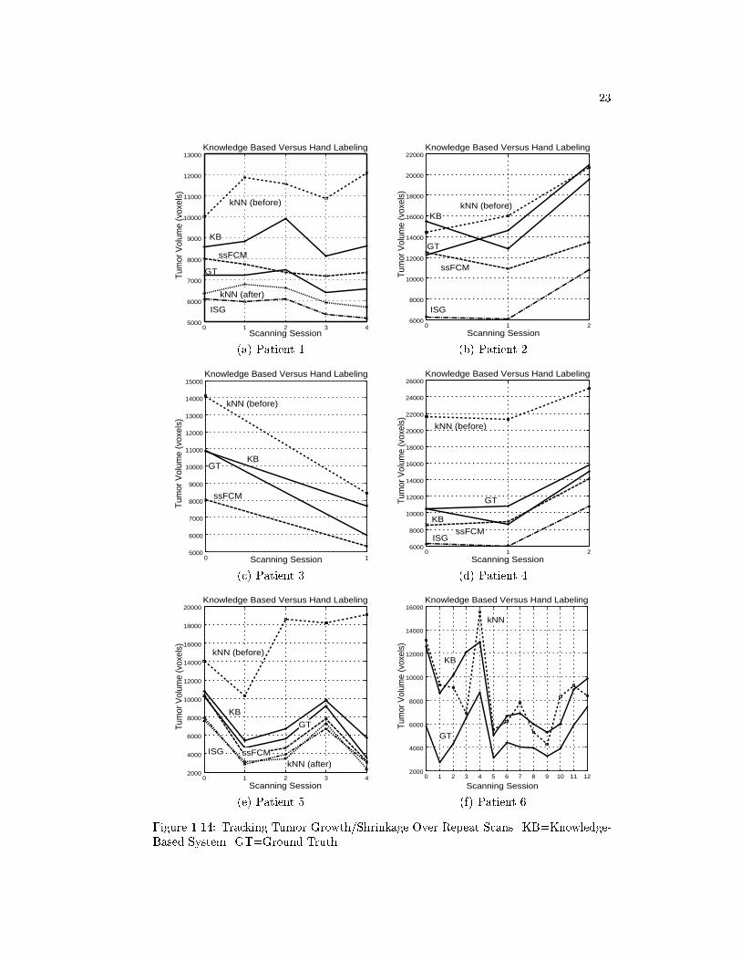
B. Evaluation Over Repeat Scans

An important use of tumor volume estimation is in tracking a tumor's response totreatment based on its growth/shrinkage. From the 33 volumes available, 25 \transi-tions" could be tracked (e.g., Baseline Scan to Repeat Scan 1 is one transition). Exam-ining tumor growth/shrinkage over repeat scans, the knowledge-based method failed toproperly track 3 of 25 transitions (12%). The kNN method, without manual tumor ex-traction, failed on 8 of 25 transitions (32%), while the manually extracted kNN volumesfailed in 2 of 10 transitions (20%). The ssFCM method failed on 3 of 13 transitions(23%), while ISG failed on 4 out of 12 (33%). Since the kNN, ssFCM, and ISG volumesare based on multiple trials, it is di�cult to assign a speci�c cause, although the im-

22

Table 1..7: Knowledge-Based Tumor vs. ssFCM and ISG. Results for Patient 6, 7, and8 for ssFCM and ISG were unavailable. (Pat. = Patient; GT Vol. = Ground TruthVolume; KB = Knowledge-based; SDP = Standard Deviation as Percentage of TumorVolume; # Trial = Number of Trials; # Obs. = Number of Observers; N/A = NotAvailable.)

Pat. Scan GT KB ssFCM ssFCM ISG ISG # #Vol. Vol. Vol. SD Vol. SD Trials Obs.

1 Base 7213 8561 8015 0.07 6067 0.05 5 2R1 7240 8829 7757 0.18 5956 0.03 5 2R2 7470 9928 7362 0.03 6087 0.03 5 2R3 6395 8132 7185 0.09 5361 0.02 5 2R4 6560 8614 7332 0.19 5172 0.04 5 2

2 Base 12230 15494 12457 0.06 10027 0.06 5 2R1 14609 12874 10916 0.13 7120 0.15 5 2R2 20924 19541 13498 0.06 10120 0.06 5 2

3 Base 10892 10855 8018 0.08 N/A N/A 5 3R1 5971 7688 5337 0.03 N/A N/A 5 3

4 Base 10454 10517 8563 0.05 6258 0.02 4 2R1 10835 8614 8901 0.04 6040 0.03 4 2R2 15788 15045 14080 0.06 10819 0.17 4 2

5 Base 10178 10784 10334 0.06 7562 0.09 4 2R1 4657 5489 3813 0.15 3142 0.24 4 2R2 5616 6773 4667 0.09 3483 0.07 4 2R3 9215 9833 7852 0.02 7300 0.06 4 2R4 3544 5730 3110 0.19 2311 0.13 4 2

23

5000

6000

7000

8000

9000

10000

11000

12000

13000

0 1 2 3 4

Tum

or V

olum

e (v

oxel

s)

Scanning Session

Knowledge Based Versus Hand Labeling

KB

GT

kNN (before)

ssFCM

ISG

kNN (after)

(a) Patient 1

6000

8000

10000

12000

14000

16000

18000

20000

22000

0 1 2

Tum

or V

olum

e (v

oxel

s)

Scanning Session

Knowledge Based Versus Hand Labeling

KB

GT

kNN (before)

ssFCM

ISG

(b) Patient 2

5000

6000

7000

8000

9000

10000

11000

12000

13000

14000

15000

0 1

Tum

or V

olum

e (v

oxel

s)

Scanning Session

Knowledge Based Versus Hand Labeling

KBGT

kNN (before)

ssFCM

(c) Patient 3

6000

8000

10000

12000

14000

16000

18000

20000

22000

24000

26000

0 1 2

Tum

or V

olum

e (v

oxel

s)

Scanning Session

Knowledge Based Versus Hand Labeling

KB

GT

kNN (before)

ssFCMISG

(d) Patient 4

2000

4000

6000

8000

10000

12000

14000

16000

18000

20000

0 1 2 3 4

Tum

or V

olum

e (v

oxel

s)

Scanning Session

Knowledge Based Versus Hand Labeling

KB

kNN (before)

ISG

GT

ssFCMkNN (after)

(e) Patient 5

2000

4000

6000

8000

10000

12000

14000

16000

0 1 2 3 4 5 6 7 8 9 10 11 12

Tum

or V

olum

e (v

oxel

s)

Scanning Session

Knowledge Based Versus Hand Labeling

KB

kNN

GT

(f) Patient 6

Figure 1.14: Tracking Tumor Growth/Shrinkage Over Repeat Scans. KB=Knowledge-Based System. GT=Ground Truth.

24

(a) Raw Image (b) KB Tumor (c) GT Tumor

(d) Raw Image (e) KB Tumor (f) GT Tumor

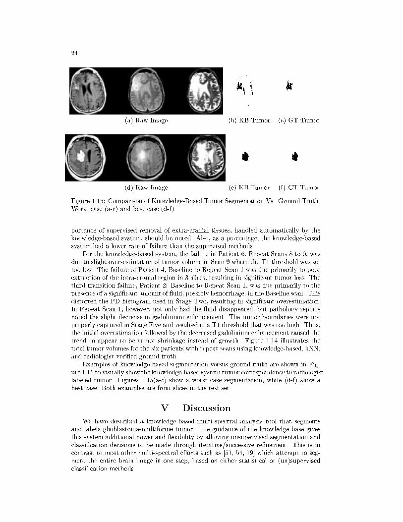
Figure 1.15: Comparison of Knowledge-Based Tumor Segmentation Vs. Ground Truth.Worst case (a-c) and best case (d-f).

portance of supervised removal of extra-cranial tissues, handled automatically by theknowledge-based system, should be noted. Also, as a percentage, the knowledge-basedsystem had a lower rate of failure than the supervised methods.

For the knowledge-based system, the failure in Patient 6, Repeat Scans 8 to 9, wasdue to slight over-estimation of tumor volume in Scan 9 where the T1 threshold was settoo low. The failure of Patient 4, Baseline to Repeat Scan 1 was due primarily to poorextraction of the intra-cranial region in 3 slices, resulting in signi�cant tumor loss. Thethird transition failure, Patient 2: Baseline to Repeat Scan 1, was due primarily to thepresence of a signi�cant amount of uid, possibly hemorrhage, in the Baseline scan. Thisdistorted the PD histogram used in Stage Two, resulting in signi�cant overestimation.In Repeat Scan 1, however, not only had the uid disappeared, but pathology reportsnoted the slight decrease in gadolinium enhancement. The tumor boundaries were notproperly captured in Stage Five and resulted in a T1 threshold that was too high. Thus,the initial overestimation followed by the decreased gadolinium enhancement caused thetrend to appear to be tumor shrinkage instead of growth. Figure 1.14 illustrates thetotal tumor volumes for the six patients with repeat scans using knowledge-based, kNN,and radiologist-veri�ed ground truth.

Examples of knowledge-based segmentation versus ground-truth are shown in Fig-ure 1.15 to visually show the knowledge-based system tumor correspondence to radiologist-labeled tumor. Figures 1.15(a-c) show a worst case segmentation, while (d-f) show abest case. Both examples are from slices in the test set.

V. Discussion

We have described a knowledge-based multi-spectral analysis tool that segmentsand labels glioblastoma-multiforme tumor. The guidance of the knowledge base givesthis system additional power and exibility by allowing unsupervised segmentation andclassi�cation decisions to be made through iterative/successive re�nement. This is incontrast to most other multi-spectral e�orts such as [51, 54, 19] which attempt to seg-ment the entire brain image in one step, based on either statistical or (un)supervisedclassi�cation methods.

25

The knowledge base was initially built with a general set of heuristics comparing thee�ects of di�erent pulse sequences on di�erent types of tissues. This process is called\knowledge-engineering" as we had to decide which knowledge was most useful for thegoal of tumor segmentation, followed by the process of implementing such informationinto a rule-based system. More importantly, the training set used was quite small -seventeen slices over three patients. Yet, the system performed well. A larger trainingset would most likely allow new and more e�ective trends and characteristics to berevealed. Thresholds used to handle a certain subset of the training set could be bettergeneralized.

The slices processed had a relatively large thickness of 5mm. Thinner slices whichexhibit a reduced partial-volume e�ect and allow better tissue contrast could be used.While relying on feature space distributions, the system was developed using generaltissue characteristics and relative relationships between tissues to avoid dependenceupon speci�c feature-domain values. The particular slices were acquired with the sameparameters, but gadolinium-enhancement has been found to be generally very robustin di�erent protocols and thickness [4, 24]. Should acquisition parameter dependencebecome an issue, given a large enough training base across multiple parameters, theknowledge base could automatically adjust to a slice's speci�c parameters since such in-formation is easily included when processing starts. The patient volumes processed hadreceived various degrees of treatment, including surgery, radiation and chemo-therapyboth before and between scans. Yet, despite the changes these treatments can cause,such as demyelinization of white matter, no modi�cations to the knowledge based sys-tem were necessary. Other approaches, like neural networks [1] or any sort of supervisedmethod which is based on a speci�c set of training examples could have di�culties indealing with slightly di�erent imaging protocols and the e�ects of treatment.

The promise of the knowledge-based system as a useful tool is demonstrated by thesuccessful performance of the system on the processed slices. The �nal KB segmen-tations compare well with radiologist-labeled \ground truth" images. The knowledge-based system also compared well with supervised methods, and was able to segmenttumor without the need for (multiple) human-based ROI's or post-processing, whichmake supervised methods clinically impractical.

As stated in the introduction, no method of quantitating tumor volumes is widelyaccepted and used in clinical practice [38]. An method by the Eastern CooperativeOncology group [17] approximates tumor area in the single MR slice with the largestcontiguous, well-de�ned tumor evident. The longest tumor diameter is multiplied byits perpendicular to yield an area. Changes greater than 25% in the area of a tumorover time are used, in conjunction with visual observations, to classify tumor responseto treatment into �ve categories from complete response (no measurable tumor left) toprogression. This approach does not address full tumor volume, depends on the exactboundary choices, and the shape of the tumor [31, 17]. By itself, the approach can leadto inaccurate growth/shrinkage decisions [10].

Overall, the knowledge-based approach tended to overestimate the tumor volume.Only two patients (2 and 4) showed noticeable underestimation by the knowledge-basedsystem. In all other cases, the knowledge-based system shows a number of \false pos-itives." Since the system segments tumor by removing only pixels proven not to betumor, leaving anything that remains being labeled as tumor, a higher level of falsepositives is not inconsistent with the paradigm. The �nal T1 threshold is applied us-ing a �xed parameter �, but the knowledge-based system's errors suggest that creatingrules to automatically set � (making Stage Five more adaptive to tumors with di�erentdegrees of enhancement) is worthy of investigation.

It should also be noted, however, that the process of creating ground truth images

26

is very imprecise [40] and has approximately a 5% inter-observer variability in tumorvolume [56]. All brain tumors have micro-in�ltration beyond the borders de�ned withgadolinium enhancement. This is especially true in glioblastoma-multiformes, whichare the most aggressive grade of primary glioma brain tumors, and no one can tell theexact tumor borders, even with invasive histopathological methods [9, 18, 41], whichwere unavailable. Ground truth images mark the areas of tumor exhibiting the mostangiogenesis (formation of blood vessels, resulting in the greatest gadolinium concen-tration) and represent those pixels which are \statistically most likely" to contain tu-mor [40, 41]. Such pixels would have the highest level of agreement agreement betweenradiologists, but they do not guarantee that all tumor has been identi�ed [40]. There-fore, the knowledge-based system may often capture tumor boundaries that extendinto areas showing lower degrees of angiogenesis (which would still be treated duringtherapy) [41].

Future work includes addressing the problems noted in Section IV. to improve thesystem's performance. The high number of false positives, which appear to be a matterof tumor boundaries, can be reduced by applying a �nal threshold in T1-space (thefeature image used primarily by radiologists in determining �nal tumor boundaries).Our primary concern was losing as little ground truth tumor as possible. Expanding thetraining set to include more patients should expand the generalizability of the knowledgebase. The next expected development in this system is to expand the processing rangeto all slices that intersect the brain cerebrum. Introducing new tumor types, such aslower grade gliomas will also be considered, as will complete labeling of all remainingtissues. Also, newer MRI systems may provide additional features, such as di�usionimages or edge strength to estimate tumor boundaries, which can be readily includedinto the knowledge base. The knowledge-base also allows straightforward expansion asnew tools are found e�ective.

In conclusion, the knowledge-based system is a multi-spectral tool that shows promisein e�ectively segmenting glioblastoma-multiforme tumors without the need for humansupervision. It has the potential of being a useful tool for segmenting tumor for therapyplanning, and tracking tumor response. Lastly, the knowledge-based paradigm allowseasy integration of new domain information and processing tools into the existing sys-tem when other types of pathology and MR data are considered.

Acknowledgements

This research was partially supported by a grant from the Whitaker foundationand a grant from the National Cancer Institute (CA59 425-01). Thanks to Dr. MohanVaidyanathan for his assistance in the ground truth work.

References[1] Amartur, S., Piriano, D., and Takefuji, Y. Optimization neural networks

for the segmentation of magnetic resonance images. IEEE TMI 11, 2 (June 1992),215{221.

[2] Bomans, M., H�ohne, K., Tiede, U., and Riemer, M. 3D segmentation ofMR images of the head for 3D display. IEEE TMI 9 (1990), 177{183.

[3] Bottomley, P., Foster, T., Argersinger, R., and Pfei�er, L. A review ofnormal tissue hydrogen NMR relaxation times and relaxation mechanisms from1-100 MHz: Dependency on tissue type, NMR frequency, temperature, species,excision and age. Medical Physics 11 (1984), 425{448.

27

[4] Bronen, R., and Sze, G. Magnetic resonance imaging contrast agents: Theoryand application to the central nervous system. Journal of Neurosurgery 73 (1990),820{839.

[5] Cannon, R., Dave, J., and Bezdek, J. E�cient implementation of the fuzzyc-mean clustering algorithms.IEEE Transactions on Pattern Analysis and MachineIntelligence 8, 2 (1986), 248{255.

[6] Clark, M., Hall, L., Goldgof, D., and et al. MRI segmentation using fuzzyclustering techniques: Integrating knowledge. IEEE Engineering in Medicine andBiology 13, 5 (1994), 730{742.

[7] Clark, M., Hall, L., Li, C., and Goldgof, D. Knowledge based (re-)clustering.In Proceedings of the 12th IAPR International Conference on Pattern Recognition(1994), pp. 245{250. Jerusalem, Israel.

[8] Clark, M. C.Knowledge-Guided Processing of Magnetic Resonance Images of theBrain. PhD thesis, University of South Florida, 1997.

[9] Clarke, L., Velthuizen, R., Camacho, M., Heine, J., Vaydianathan, M.,

Hall, L., Thatcher, R., and Silbiger, M. MRI segmentation: Methods andapplications. Magnetic Resonance Imaging 13, 3 (1995), 343{368.

[10] Clarke, L., Velthuizen, R., Clark, M., Gaviria, G., Hall, L., Goldgof,

D., and et al. MRI measurement of brain tumor response: Comparison of visualmetric and automatic segmentation. Submitted to Magnetic Resonance Imaging,June 1997.

[11] Dasarthy, B. Nearest Neighbor (NN) Norms: NN Pattern Classi�cation Tech-niques. IEEE Computer Society Press, Los Alamitos, Ca., 1991.

[12] Dellepiane, S. Image segmentation: Errors, sensitivity, and uncertainty. InProceedings of the 13th IEEE EMB Society (1991), vol. 13, pp. 253{254.

[13] Dellepiane, S., Venturi, G., and Vernazza, G. A fuzzy model for the process-ing and recognition of MR pathological images. In IPMI 1991 (1991), pp. 444{457.

[14] Dougherty, S. Discussions held with Sean Dougherty concerning edge detectionalgorithms in MR images, September 1997.

[15] Farrar, T. C. An Introduction to Pulse NMR Spectroscopy. Farragut Press, 1987.

[16] Feldman, G. B. Brain tumor facts and �gures. The Brain Tumor Society -http://www.thts.org/btfacts.htm, July 3 1997.

[17] Feun, L. Double-blind randomized trial of the anti-progestational agent mifepri-stone in the treatment of unresectable meningioma, phase iii. Tech. Rep. SWOG-9005, University of South Florida, Tampa, Fl., Southwest Oncology Group, 1995.

[18] Galloway, R., Maciunas, R., and Failinger, A. Factors a�ecting perceivedtumor volumes in magnetic resonance imaging. Annals of Biomedical Engineering21 (1993), 367{375.

[19] Gerig, G., Martin, J., Kikinis, R., and et al. Automating segmentation ofdual-echo MR head data. In The 12th International Conference of InformationProcessing in Medical Imaging (IPMI 1991) (1991).

[20] Giarratano, J., and Riley, G. Expert Systems: Principles and Programming,second ed. Boston: PWS Publishing, 1994.

[21] Gibbs, P., Buckley, D., Blackband, S., and Horsman, A. Tumor volumedetermination fromMR images by morphological segmentation.Physics in Medicineand Biology 41, 11 (November 1996), 2437{2446.

[22] Gong, L., and Kulikowski, C. Automatic segmentation of brain images: Selec-tion of region extraction methods. In SPIE Vol. 1450 Biomedical Image ProcessingII (1991), SPIE, pp. 144{153.

28

[23] Hall, L., Bensaid, A., Clarke, L., and et al. A comparison of neural networkand fuzzy clustering techniques in segmenting magnetic resonance images of thebrain. IEEE Transactions on Neural Networks 3, 5 (1992), 672{682.

[24] Hendrick, R., and Haacke, E. Basic physics of MR contrast agents and maxi-mization of image contrast. JMRI 3, 1 (1993), 137{148.

[25] Hillman, G., Chang, C., Ying, H., and et al. Automatic system for brain MRIanalysis using a novel combination of fuzzy rule-based and automatic clusteringtechniques. In Medical Imaging 1995: Image Processing (February 1995), SPIE,pp. 16{25. San Diego, CA.

[26] Jain, A. Fundamentals of Digital Image Processing. Englewood Cli�s,NJ: PrenticeHall, 1989.

[27] Jain, R., Kasturi, R., and Schunck, B. Machine Vision. McGraw-Hill, Inc.,1995.

[28] Kamber, M., Shingal, R., Collins, D., Francis, G., and Evans, A. Model-based 3D segmentation of multiple sclerosis lesions in magnetic resonance brainimages. IEEE TMI 14, 3 (1995), 442{453.

[29] Kikinis, R., Shenton, M., Gerig, G., and et al. Routine quantitative analysisof brain and cerebrospinal uid spaces with MR imaging. JMRI 2 (1992), 619{629.

[30] Kischell, E., Kehtarnavaz, N., Hillman, G., Levin, H., Lilly, M., and

Kent, T. Classi�cation of brain compartments and head injury lesions by neuralnetworks applied to MRI. Neuroradiology 37 (1995), 535{541.

[31] Laperrire, N., and Berstein, M.Radiotherapy for brain tumors.CA - A CancerJournal for Clinicians 4 (1994), 96{108.

[32] Leeds, N., and Jackson, E. Current imaging techniques for the evaluation ofbrain neoplasms. Current Science 6 (1994), 254{261.

[33] Li, C. Knowledge based classi�cation and tissue labeling of magnetic resonanceimages of the brain. Master's thesis, University of South Florida, 1993.

[34] Li, C., Goldgof, D., and Hall, L. Automatic segmentation and tissue labelingof MR brain images. IEEE TMI 12, 4 (December 1993), 740{750.

[35] Li, X., Bhide, S., and Kabuka, M. Labeling of MR brain images using booleanneural network. IEEE TMI 15, 2 (1996), 628{638.

[36] Lufkin, R. B. The MRI Manual. Year Book Medical Publishers, Inc., 1990.

[37] Menhardt, W., and Schmidt, K. Computer vision on magnetic resonanceimages. Pattern Recognition Letters 8, 2 (September 1988), 73{85.

[38] Murtagh, R., Phuphanich, S., Imam, N., Clarke, L., Vaidyanathan, M.,

and et.al. Novel methods of evaluating the growth response patterns of treatedbrain tumors. Cancer Control (1995), 293{299.

[39] Murtaugh, F. Discussions held with Dr. F. Reed Murtaugh, M.D., Dept. ofRadiology, University of South Florida, April 1997.

[40] Murtaugh, F. Discussions held with Dr. F. Reed Murtaugh, M.D., Dept. ofRadiology, University of South Florida, October, 1 1997.

[41] Murtaugh, F. Discussions held with Dr. F. Reed Murtaugh, M.D., Dept. ofRadiology, University of South Florida, October, 22 1997.

[42] Namasivayam, A., and Hall, L. Integrating fuzzy rules into the fast, robustsegmentation of magnetic resonance images. In New Frontiers in Fuzzy Logic andSoft Computing Biennial Conference of the North American Fuzzy InformationProcessing Society - NAFIPS 1996 (1996), pp. 23{27. Piscataway, NJ.

[43] Novelline, R., and Squire, L. Living Anatomy. Hanley and Belfus, 1987.

29

[44] �Ozkan, M., Dawant, B., and Maciunas, R. Neural-network-based segmenta-tion of multi-modal medical images: A comparative and prospective study. IEEETMI 12, 3 (September 1993), 534{545.

[45] Ra�, U., and Newman, F. Automated lesion detection and lesion quantitationin MR images using autoassociative memory. Medical Physics 19 (1992), 71{77.

[46] Riley, G. Version 4.3 CLIPS reference manual. Tech. Rep. JSC-22948, Arti�cialIntelligence Section, Lyndon B. Johnson Space Center, 1989.

[47] Schnitzlein, H., and Murtaugh, F. R.Imaging Anatomy of the Head and Spine:A Photographic Color Atlas of MRI, CT, Gross, and Microscopic Anatomy in Axial,Coronal, and Sagittal Planes, second ed. Baltimore: Urban & Schwarzenberg, 1990.

[48] Stark, D. D., and William G. Bradley, J. Magnetic Resonance Imaging,Second Ed., Volume One. Mosby Year Book, 1992.

[49] Tao, C., and Thompson, W.A fuzzy if-then approach to edge detection. In 1993IEEE International Conference on Fuzzy Systems (1993), IEEE, pp. 1356{1360.

[50] Taxt, T., and Lundervold, A. Multispectral analysis of the brain in mag-netic resonance imaging. In IEEE Workshop on Biomedical Image Analysis (1994),pp. 33{42. Los Alamitos, CA, USA.

[51] Taxt, T., and Lundervold, A.Multispectral analysis of the brain using magneticresonance imaging. IEEE TMI 13, 3 (September 1994), 470{481.

[52] Vaidyanathan, M., Velthuizen, R., Clarke, L., and Hall, L. Quantitationof brain tumor in MRI for treatment planning. In Proceedings of the 16th AnnualInternational Conference of the IEEE Engineering in Medicine and Biology Society(1994), vol. 16, pp. 555{556.

[53] Vaidyanathan, M., Velthuizen, R., Venugopal, P., and Clarke, L. Tu-mor volume measurements using supervised and semi-supervised MRI segmenta-tion methods. In Arti�cial Neural Networks in Engineering - Proceedings (ANNIE1994) (1994), vol. 4, pp. 629{637.

[54] Vannier, M., Butter�eld, R., Jordan, D., and et al. Multispectral analysisof magnetic resonance images. Radiology 154, 1 (January 1985), 221{224.

[55] Vannier, M., Speidel, C., and Rickmans, D. Magnetic resonance imagingmultispectral tissue classi�cation. News Physiol Sci 3 (August 1988), 148{154.

[56] Velthuizen, R., and Clarke, L.An interface for validation of MR image segmen-tations. In Proceedings of the 16th Annual International Conference of the IEEEEngineering in Medicine and Biology Society (1994), pp. 547{548.

[57] Velthuizen, R., Hall, L., and Clarke, L. Unsupervised fuzzy segmentation of3D magnetic resonance brain images. In Proceedings of the IS&TSPIE 1993 Inter-national Symposium on Electronic Images: Science & Technology (1993), vol. 1905,pp. 627{635. San Jose, CA, Jan 31-Feb 4.

[58] Velthuizen, R., Phuphanich, S., Clarke, L., Hall, L., and et al.Unsupervisedtumor volume measurement using magnetic resonance brain images. JMRI 5, 5(1995), 594{605.

[59] Wu, Z., and Leahy, R. A graph theoretic approach to segmentation of MRimages. In SPIE Vol.1450 Biomedical Image Processing II (1991), pp. 120{132.

[60] Wu, Z., and Leahy, R. Image segmentation via edge contour �nding: A graphtheoretic approach. In IEEE Computer Vision and Pattern Recognition (1992),pp. 613{619.