vehicle modeling and adams-simulink
DESCRIPTION
helpTRANSCRIPT
VEHICLE MODELING AND ADAMS-SIMULINK CO-SIMULATION WITH
INTEGRATED CONTINUOUSLY CONTROLLED ELECTRONIC SUSPENSION
(CES) AND ELECTRONIC STABILITY CONTROL (ESC) MODELS
A Thesis
Presented in Partial Fulfillment of the Requirements for
the Degree of Master of Science in the
Graduate School of The Ohio State University
By
Sughosh Jagannatha Rao, B.S.M.E
********
The Ohio State University
2009
Masters Examination Committee: Approved By: Prof. Dennis A. Guenther, Advisor ____________________ Advisor Dr. Gary J. Heydinger Graduate Program in Mechanical Engineering

ii
ABSTRACT
The purpose of this thesis is to evaluate the benefits of the CES suspension system
developed by Tenneco Automotive, and to evaluate the effects of the CES suspension on
the Electronic Stability Control (ESC) system using ADAMS simulation. The design of
the system and its function is explained.
The first stage of the process involved the creation of the ADAMS model of the
Ford Expedition. Next, the model was validated from the Expedition model used with the
National Advanced Driving Simulator (NADS) and experimental data collected at
Transportation Research Center (TRC). Once the vehicle model was ready, a model of
the ESC system was created using Matlab Simulink. Next, a co-simulation was set up to
integrate the ESC model with the vehicle model. The ESC equipped vehicle model was
then validated against experimental data.
The CES model supplied by Tenneco Automotive was then incorporated into the
validated model. This model was then used to evaluate the performance of the baseline
Ford Expedition and one equipped with the CES suspension system. The Sine with Dwell
maneuver was used to evaluate the ESC performance in both the cases in accordance with
the Federal Motor Vehicle Safety Standard No.126 (FMVSS No.126).

iii
DEDICATION
Dedicated to my Parents,
who are the reason I am here and
have ensured that I always had all I needed and more
To all of my family; my grandparents, uncles, aunts, cousins and friends,
for all of your love and support.

iv
ACKNOWLEGMENTS
I would like to offer thanks to a lot of people, without whom this study would not
have been possible. I would like to thank my advisors, Denny Guenther, Gary Heydinger
and Kamel Salaani for their support and constant encouragement which got me through
some really hard patches when progress was slow. More than advisors, they were like
friends, always there to answer my questions and lend a helping hand. Throughout the
project, they ensured that they did not put any unnecessary pressure. I would like to
especially thank Denny, for always keeping my interests in mind and making me feel at
home. I would also like to thank Tenneco Automotive for supporting this research with
both monetary and technical contributions, without their project, I would not be writing
this thesis.
I would also like to thank my colleagues Tejas Kinjawadekar and Neha Dixit who
kept me company and helped keep the stress low. I would also like to thank Don Butler
and Luka Wahab for their help. Thanks to my friends and roommates who have made this
journey fun and full of fond memories. Finally I would like to thank my family, without
their support and belief; this would not have been possible. Without the support of all the
people mentioned here, the completion of my Masters Degree would not have been
possible.
v
VITA
15 May 1985……………………Born – Mysore, India
June 2002……………………….Graduate, DAV Higher Sec. School
May 2006……………………….B.E.M.E. Anna University
Sept. 2006 – Aug 2007…………University Fellow, The Ohio State University
Sept. 2007 – Present……………Graduate Research Assistant, The Ohio State University
FIELDS OF STUDY
Major Field: Mechanical Engineering Vehicle Dynamics

vi
TABLE OF CONTENTS
ABSTRACT........................................................................................................................ ii
DEDICATION................................................................................................................... iii
ACKNOWLEGMENTS .................................................................................................... iv
VITA................................................................................................................................... v
TABLE OF CONTENTS................................................................................................... vi
LIST OF FIGURES ........................................................................................................... ix
LIST OF TABLES........................................................................................................... xiv
1 INTRODUCTION ...................................................................................................... 1
1.1 Motivation........................................................................................................... 1
1.2 Modeling/Simulation .......................................................................................... 3
1.3 Thesis Outline ..................................................................................................... 3
1.3.1 First Objective – Create Vehicle Model in Adams View ........................... 3
1.3.2 Second Objective – Create ESC model using Simulink ............................. 4
1.3.3 Third Objective – Setup Adams and Simulink Co-Simulation................... 4
1.3.4 Fourth Objective – Simulate Maneuvers on the Model .............................. 4
1.3.5 Fifth Objective – Obtain and Analyze Simulation Data ............................. 5
2 MODELING ............................................................................................................... 6
2.1 Overview............................................................................................................. 6
2.2 Hard Point Locations .......................................................................................... 6

vii
2.3 Multibody Model and Inertia Properties........................................................... 10
2.4 Springs and Shock Absorbers ........................................................................... 14
2.5 Tires and Road .................................................................................................. 14
2.6 Drive Train........................................................................................................ 15
2.7 Modeling Measures........................................................................................... 15
2.7.1 Wheel Camber Angle................................................................................ 15
2.7.2 Front Wheel Steer Angle .......................................................................... 16
2.7.3 Roll Angle................................................................................................. 16
2.7.4 Accelerometer Readings ........................................................................... 17
3 VALIDATION.......................................................................................................... 18
3.1 Introduction....................................................................................................... 18
3.2 Quasi-Static Tests ............................................................................................. 18
3.2.1 Bounce Tests............................................................................................. 18
3.2.2 Roll Test.................................................................................................... 23
3.2.3 Steering Ratio Test.................................................................................... 27
3.3 Dynamic Maneuvers ......................................................................................... 28
3.3.1 Slowly Increasing Steer Maneuver ........................................................... 28
3.3.2 Sine with Dwell Maneuver ....................................................................... 33
4 CO-SIMULATION................................................................................................... 43
4.1 Overview........................................................................................................... 43
4.2 Input and Output Variables............................................................................... 44
4.3 Setting up the Co-simulation ............................................................................ 46
4.3.1 Loading Adams/Controls .......................................................................... 46

viii
4.3.2 Defining Input and Output Variables........................................................ 47
4.3.3 Referencing Input Variables ..................................................................... 49
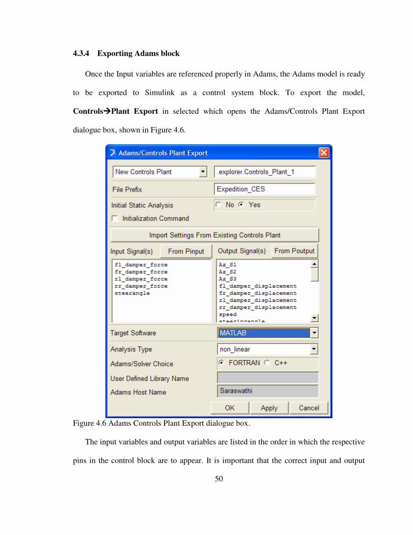
4.3.4 Exporting Adams block ............................................................................ 50
4.3.5 Connecting the Adams Block and the CES Block in Simulink. ............... 51
4.3.6 Running the Co-simulation ....................................................................... 55
4.3.7 Things to Remember................................................................................. 56
5 ELECTRONIC STABILITY CONTROL ................................................................ 57
5.1 Overview........................................................................................................... 57
5.2 ESC Model........................................................................................................ 58
5.3 Validation.......................................................................................................... 61
6 CONTINUOUSLY CONTROLLED ELECTRONIC SUSPENSION (CES)
SYSTEM........................................................................................................................... 73
6.1 Introduction....................................................................................................... 73
6.2 Results............................................................................................................... 74
6.3 Conclusion ........................................................................................................ 87
7 CONCLUSIONS AND RECOMMENDATIONS ................................................... 88
7.1 Conclusions....................................................................................................... 88
7.2 Recommendations............................................................................................. 89
REFERENCES ................................................................................................................. 91
ix
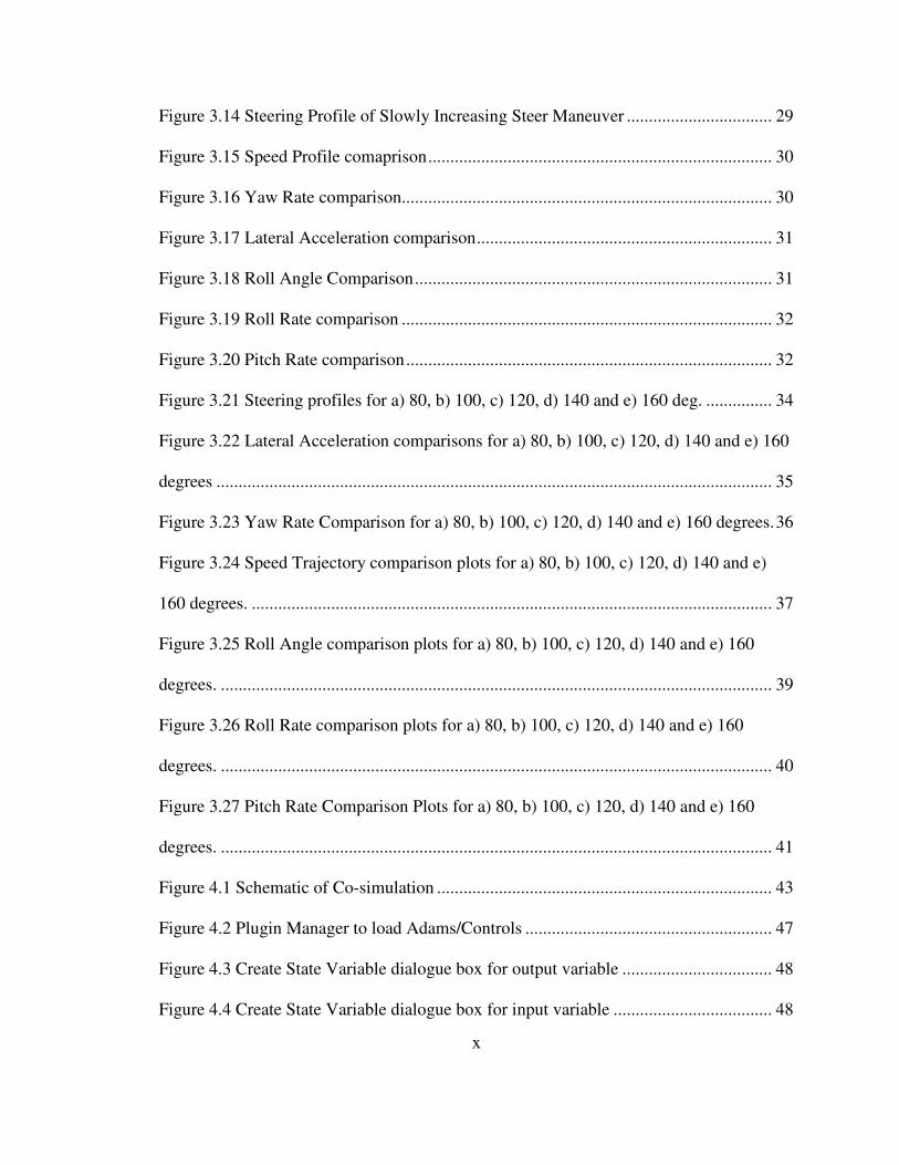
LIST OF FIGURES
Figure 2.1 Rear suspension roll stability bar ...................................................................... 8
Figure 2.2 Front Roll stability bar....................................................................................... 9
Figure 2.3 Adams Model of the Ford Expedition............................................................. 11
Figure 2.4 Topology map of Ford Expedition model. ...................................................... 12
Figure 2.5 Vertical Acceleration Measure of Accelerometer ........................................... 17
Figure 3.1 Front Suspension Spring Rate plot .................................................................. 19
Figure 3.2 Front Suspension Bounce Steer plot................................................................ 20
Figure 3.3 Front Suspension Bounce Camber plot ........................................................... 20
Figure 3.4 Rear Suspension Spring Rate plot ................................................................... 21
Figure 3.5 Rear Suspension Bounce Steer plot................................................................. 22
Figure 3.6 Rear Suspension Bounce Camber plot ............................................................ 22
Figure 3.7 Front Overall Roll Stiffness plot ..................................................................... 24
Figure 3.8 Front Roll Steer plot ........................................................................................ 24
Figure 3.9 Front Roll Camber Angle plot ......................................................................... 25
Figure 3.10 Rear Overall Roll Stiffness plot .................................................................... 26
Figure 3.11Rear Roll Steer plot ........................................................................................ 26
Figure 3.12 Rear Roll Camber plot................................................................................... 27
Figure 3.13 Steering Ratio Test plot of the model............................................................ 28
x
Figure 3.14 Steering Profile of Slowly Increasing Steer Maneuver ................................. 29
Figure 3.15 Speed Profile comaprison.............................................................................. 30
Figure 3.16 Yaw Rate comparison.................................................................................... 30
Figure 3.17 Lateral Acceleration comparison................................................................... 31
Figure 3.18 Roll Angle Comparison................................................................................. 31
Figure 3.19 Roll Rate comparison .................................................................................... 32
Figure 3.20 Pitch Rate comparison................................................................................... 32
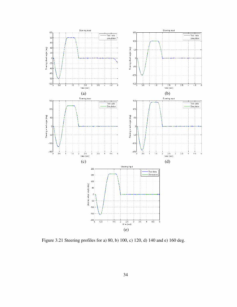
Figure 3.21 Steering profiles for a) 80, b) 100, c) 120, d) 140 and e) 160 deg. ............... 34
Figure 3.22 Lateral Acceleration comparisons for a) 80, b) 100, c) 120, d) 140 and e) 160
degrees .............................................................................................................................. 35
Figure 3.23 Yaw Rate Comparison for a) 80, b) 100, c) 120, d) 140 and e) 160 degrees.36
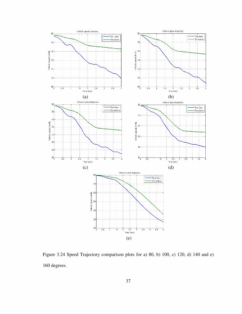
Figure 3.24 Speed Trajectory comparison plots for a) 80, b) 100, c) 120, d) 140 and e)
160 degrees. ...................................................................................................................... 37
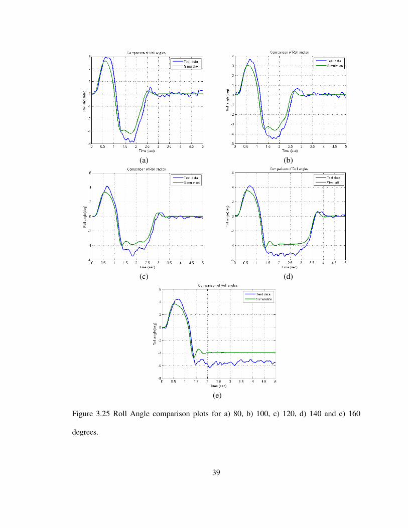
Figure 3.25 Roll Angle comparison plots for a) 80, b) 100, c) 120, d) 140 and e) 160
degrees. ............................................................................................................................. 39
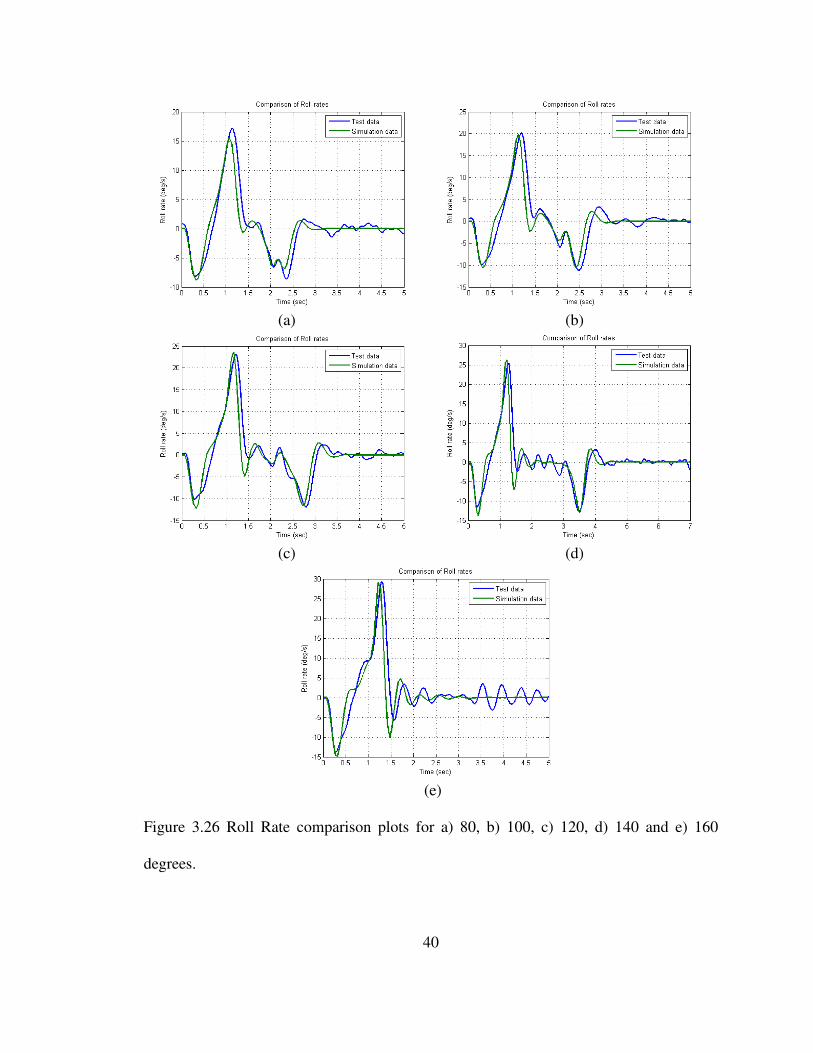
Figure 3.26 Roll Rate comparison plots for a) 80, b) 100, c) 120, d) 140 and e) 160
degrees. ............................................................................................................................. 40
Figure 3.27 Pitch Rate Comparison Plots for a) 80, b) 100, c) 120, d) 140 and e) 160
degrees. ............................................................................................................................. 41
Figure 4.1 Schematic of Co-simulation ............................................................................ 43
Figure 4.2 Plugin Manager to load Adams/Controls ........................................................ 47
Figure 4.3 Create State Variable dialogue box for output variable .................................. 48
Figure 4.4 Create State Variable dialogue box for input variable .................................... 48
xi
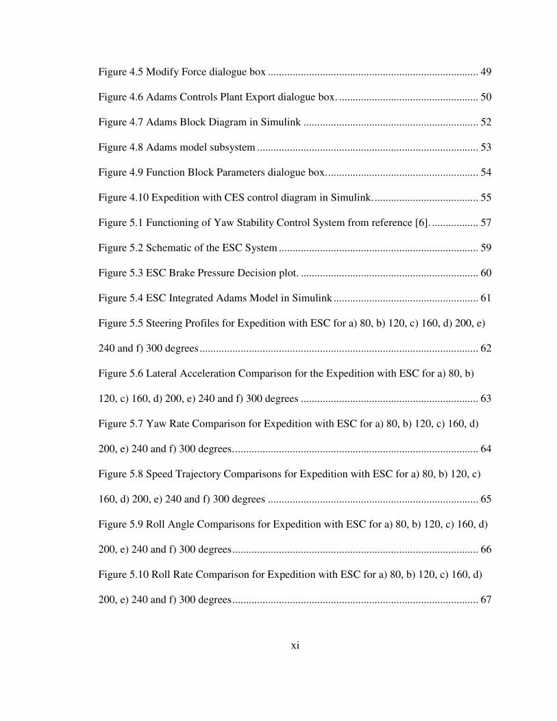
Figure 4.5 Modify Force dialogue box ............................................................................. 49
Figure 4.6 Adams Controls Plant Export dialogue box. ................................................... 50
Figure 4.7 Adams Block Diagram in Simulink ................................................................ 52
Figure 4.8 Adams model subsystem ................................................................................. 53
Figure 4.9 Function Block Parameters dialogue box........................................................ 54
Figure 4.10 Expedition with CES control diagram in Simulink....................................... 55
Figure 5.1 Functioning of Yaw Stability Control System from reference [6]. ................. 57
Figure 5.2 Schematic of the ESC System ......................................................................... 59
Figure 5.3 ESC Brake Pressure Decision plot. ................................................................. 60
Figure 5.4 ESC Integrated Adams Model in Simulink ..................................................... 61
Figure 5.5 Steering Profiles for Expedition with ESC for a) 80, b) 120, c) 160, d) 200, e)
240 and f) 300 degrees...................................................................................................... 62
Figure 5.6 Lateral Acceleration Comparison for the Expedition with ESC for a) 80, b)
120, c) 160, d) 200, e) 240 and f) 300 degrees ................................................................. 63
Figure 5.7 Yaw Rate Comparison for Expedition with ESC for a) 80, b) 120, c) 160, d)
200, e) 240 and f) 300 degrees.......................................................................................... 64
Figure 5.8 Speed Trajectory Comparisons for Expedition with ESC for a) 80, b) 120, c)
160, d) 200, e) 240 and f) 300 degrees ............................................................................. 65
Figure 5.9 Roll Angle Comparisons for Expedition with ESC for a) 80, b) 120, c) 160, d)
200, e) 240 and f) 300 degrees.......................................................................................... 66
Figure 5.10 Roll Rate Comparison for Expedition with ESC for a) 80, b) 120, c) 160, d)
200, e) 240 and f) 300 degrees.......................................................................................... 67
xii
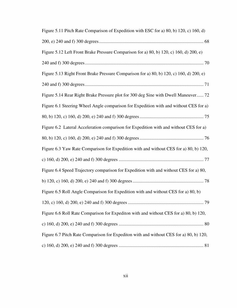
Figure 5.11 Pitch Rate Comparison of Expedition with ESC for a) 80, b) 120, c) 160, d)
200, e) 240 and f) 300 degrees.......................................................................................... 68
Figure 5.12 Left Front Brake Pressure Comparison for a) 80, b) 120, c) 160, d) 200, e)
240 and f) 300 degrees...................................................................................................... 70
Figure 5.13 Right Front Brake Pressure Comparison for a) 80, b) 120, c) 160, d) 200, e)
240 and f) 300 degrees...................................................................................................... 71
Figure 5.14 Rear Right Brake Pressure plot for 300 deg Sine with Dwell Maneuver...... 72
Figure 6.1 Steering Wheel Angle comparison for Expedition with and without CES for a)
80, b) 120, c) 160, d) 200, e) 240 and f) 300 degrees ....................................................... 75
Figure 6.2 Lateral Acceleration comparison for Expedition with and without CES for a)
80, b) 120, c) 160, d) 200, e) 240 and f) 300 degrees ....................................................... 76
Figure 6.3 Yaw Rate Comparison for Expedition with and without CES for a) 80, b) 120,
c) 160, d) 200, e) 240 and f) 300 degrees ......................................................................... 77
Figure 6.4 Speed Trajectory comparison for Expedition with and without CES for a) 80,
b) 120, c) 160, d) 200, e) 240 and f) 300 degrees ............................................................. 78
Figure 6.5 Roll Angle Comparison for Expedition with and without CES for a) 80, b)
120, c) 160, d) 200, e) 240 and f) 300 degrees ................................................................. 79
Figure 6.6 Roll Rate Comparison for Expediton with and without CES for a) 80, b) 120,
c) 160, d) 200, e) 240 and f) 300 degrees ......................................................................... 80
Figure 6.7 Pitch Rate Comparison for Expediton with and without CES for a) 80, b) 120,
c) 160, d) 200, e) 240 and f) 300 degrees ......................................................................... 81
xiii
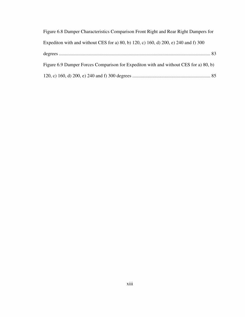
Figure 6.8 Damper Characteristics Comparison Front Right and Rear Right Dampers for
Expediton with and without CES for a) 80, b) 120, c) 160, d) 200, e) 240 and f) 300
degrees .............................................................................................................................. 83
Figure 6.9 Damper Forces Comparison for Expediton with and without CES for a) 80, b)
120, c) 160, d) 200, e) 240 and f) 300 degrees ................................................................. 85
xiv
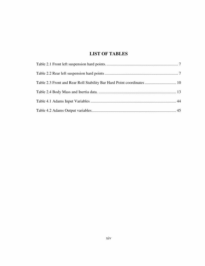
LIST OF TABLES
Table 2.1 Front left suspension hard points. ....................................................................... 7
Table 2.2 Rear left suspension hard points ......................................................................... 7
Table 2.3 Front and Rear Roll Stability Bar Hard Point coordinates ............................... 10
Table 2.4 Body Mass and Inertia data. ............................................................................. 13
Table 4.1 Adams Input Variables ..................................................................................... 44
Table 4.2 Adams Output variables.................................................................................... 45
1
CHAPTER 1:
INTRODUCTION
1.1 Motivation
Based on the 2004 Fatality Analysis Reporting Systems (FARS) and 2000-2004
National Automotive Sampling System (NASS) Crashworthiness Data System (CDS),
The National Highway Traffic Safety Administration (NHTSA) estimates that there were
34,314 police-reported passenger vehicle fatal crashes and over 2.5 million serious non-
fatal crashes (defined as at least one involved passenger vehicle was towed away). About
33,907 passenger vehicle occupant fatalities and 2,182,460 non-fatal injuries were
associated with these crashes. Single-vehicle crashes, which frequently include roadway
departure, accounted for about 53 percent (18,321 fatal crashes) of the fatal crashes and
33 percent (820,218 crashes) of the tow away crashes. A total of 15,611 occupant
fatalities and 516,500 non-fatal injuries were associated with these single-vehicle crashes.
Rollovers comprised a large share of these single-vehicle crashes and were responsible
for a disproportionate number of fatalities. Rollovers accounted for 42 percent (or 7,734
crashes) of the single-vehicle fatal crashes and 56 percent (8,487 fatalities) of the
occupant fatalities.
Single vehicle loss of control may occur when the driver attempts a sudden maneuver
(for example, to avoid an object or because one misjudged the severity of a curve), and
2
the vehicle responds differently than it does in ordinary driving as it nears the limits of
road traction.
Loss of control can result in either the rear of the vehicle “spinning out” or the front
of the vehicle “plowing out”. As long as there is sufficient road traction, a professional
race driver could maintain control in many spinout or plow out conditions by using
counter steering and other techniques. However, in a panic situation when the vehicle
begins to spin out, average drivers would be unlikely to counter steer like a race driver
and regain control. Under these circumstances, the ESC system is very effective. ESC
would potentially prevent many loss-of-control accidents from occurring and thus would
reduce associated fatalities and injuries. Based on NHTSA’s ESC effectiveness study [3]
& [4], which found that ESC is highly effective against rollovers, a large portion of these
benefits would be from rollover prevention.
Primarily, the ESC system uses automatic braking of individual wheels to adjust the
vehicle’s heading if it departs from the intended direction the driver is steering. Thus, it
prevents the heading from changing too quickly (spinning out) or not quickly enough
(plowing out) and maintains the vehicle in the direction of the heading. Although it
cannot increase the available traction, ESC controls the heading and provides sufficient
response to steering so that the driver has the maximum possibility of keeping the vehicle
on the road and avoiding obstacles in an emergency maneuver.
Over the last decade, ESC technology has advanced from just an electronic braking
control device to include other components of the vehicle like throttle control, engine
torque control and computer controlled shock absorbers to maintain stability and improve
responsiveness of the vehicle during extreme maneuvers. In their quest to constantly
3
improve the ESC performance, Tenneco Automotive has designed one such computer
controlled damper system called the Continuously Controlled Electronic Suspension
(CES) system.
The research outlined in this thesis is focused on evaluating the performance of the
CES system using simulation on a model created in Adams. The improvements in the
ESC performance due to the CES system are evaluated using the Sine with Dwell
maneuver.
1.2 Modeling/Simulation
Industries these days rely heavily on computer simulation to study the general trends
before investing heavily on actual experimental testing. Testing typically requires
multiple vehicles, numerous sets of tires and expensive instrumentation to obtain
indicative data on all the relevant parameters, and after all this there is still a possibility
that the results show that the desired results cannot be obtained thus making the whole
experiment a waste of resources. To alleviate the expenses associated, a model is first
created and simulations are run on it, to make sure that the trend shows improvement and
that one may indeed go ahead and invest in the experimentation.
1.3 Thesis Outline
1.3.1 First Objective – Create Vehicle Model in Adams View
The first portion of this thesis work involved creating a model of the Ford Expedition
in Adams View (using modeling data available from [5]). Once the model was created it
was validated using the experimental data already collected by NHTSA’s Vehicle

4
Research and Test Center (VRTC) of the basic vehicle. The Slowly Increasing Steer and
the Sine with Dwell maneuvers were used to validate the model. By varying the vehicle
compliance and tire parameters, the vehicle model was modified to provide results
consistent with real world values.
1.3.2 Second Objective – Create ESC model using Simulink
The second portion of this thesis work involved creating a black box ESC model to be
used in conjunction with the Adams vehicle model. Experimental data was used to create
look-up tables of brake pressure versus the difference in actual to desired yaw rate. This
look up table was used to create the ESC model in Simulink.
1.3.3 Third Objective – Setup Adams and Simulink Co-Simulation
The third portion of this thesis work involved setting-up the communication between
Adams and Simulink so that the ESC and CES models, both of which are modeled in
Simulink, can be incorporated into the vehicle model.
1.3.4 Fourth Objective – Simulate Maneuvers on the Model
The fourth portion of this thesis work involved simulating the Sine with Dwell
maneuver on the basic Ford Expedition with ESC and the Ford Expedition equipped with
both CES and ESC systems. The test was run for various steering wheel angles and initial
speeds of the vehicle.
5
1.3.5 Fifth Objective – Obtain and Analyze Simulation Data
The fifth part of this thesis work involved the collection and consolidation of data
from the simulations. The data was compared to determine the improvements in the
vehicle yaw response and ESC performance in the CES equipped Expedition in the
NHTSA Sine with Dwell maneuver.
6
CHAPTER 2:
MODELING
2.1 Overview
The vehicle model is created in Adams, using the graphical user interface of Adams
View. The modeling process is structured to facilitate ease of modification later in the
design, starting with creating hard points denoting the various key locations of the
suspension system. This is followed by creating links using those hard points, and finally
adding joints and constraints between the links to complete the geometry. The mass and
inertia properties are then added to the components of the suspension system.
2.2 Hard Point Locations
The SAE coordinate system was used while modeling the vehicle, with x forward, y
to the right, and z downward. The origin is located directly below the front axle and at the
middle of the track. SI units are used, i.e. meters for length, newtons for force, kilogram
for mass and seconds for time.
The data for the hard point locations were measured by SEA, Ltd. and they measured
the vehicle mass and inertia properties using their Vehicle Inertia Measurement Facility
[5]. Table 2.1 lists the hard point coordinates of the left front side suspensions hard
points. The right side hard points are coded as mirror images of left points about the x-z
7
plane. Hard-coding the right side as a mirror image of the left makes it simpler to make
changes in the suspension geometry, as changing the coordinates of a point on the left
side automatically maintains the symmetry of the right side. Table 2.2 lists the hard point
coordinates for the rear left suspension. Here again the right side is hard coded as the
mirror image of the left.
Table 2.1 Front left suspension hard points.
Table 2.2 Rear left suspension hard points
The hard point coordinates for the front and rear roll stability bars were measured
directly from the vehicle with the help of Mr. Masahiro Chuma at SEA, Ltd. Figures 2.1

8
and 2.2 show some pictures taken while the measurements were being made. The key
parts of the roll stability bar have been marked in the figures.
Figure 2.1 Rear suspension roll stability bar
a – Rear roll stability bar
b – Roll bar support, connecting the chassis to the roll bar
c – link (small rod) connecting roll bar to lower control arm

9
Figure 2.2 Front Roll stability bar
1 – Front Roll stability bar
2 – Link (small rod) connecting Roll bar to Lower control arm
3 – Support connecting roll bar to the chassis
The hard point coordinates for the front and rear anti roll bars are listed in Table 2.3.
The left side hard points are coded to be the mirror images of the right hard points about
the x-z plane.
10
Table 2.3 Front and Rear Roll Stability Bar Hard Point coordinates
2.3 Multibody Model and Inertia Properties
The suspension parts are created using the cylinder member in the Adams View tool
box. The hard points already created mark the end points of each of the suspension links,
these points are used to create the suspension geometry. Each suspension element is
modeled as a separate part, connected to other parts through joints. Figure 2.3 shows the
Ford Expedition model in Adams View. For clarity, the graphics of the Expedition body
are not modeled; however, the mass and inertia properties of the body are incorporated in
the model.
The Expedition employs a Double A-arm suspension on all four wheels. For each
wheel a lower control arm, upper control arm and knuckle are modeled as parts. The
upper and lower control arms are connected to the chassis with bushings and to the
knuckles with spherical joints. The bushings are used to introduce some steering
compliance and they are modeled to be extremely stiff in the vertical and longitudinal
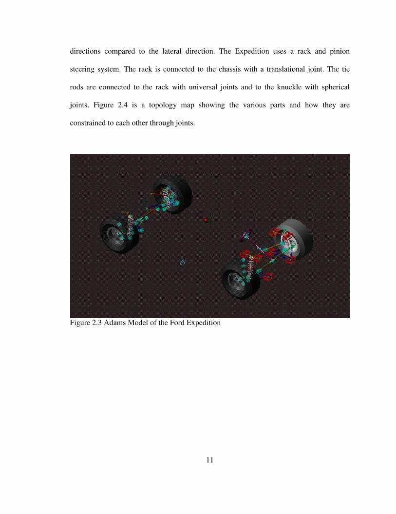
11
directions compared to the lateral direction. The Expedition uses a rack and pinion
steering system. The rack is connected to the chassis with a translational joint. The tie
rods are connected to the rack with universal joints and to the knuckle with spherical
joints. Figure 2.4 is a topology map showing the various parts and how they are
constrained to each other through joints.
Figure 2.3 Adams Model of the Ford Expedition
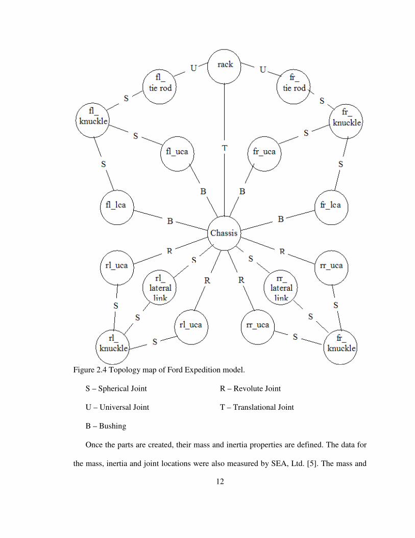
12
Figure 2.4 Topology map of Ford Expedition model.
S – Spherical Joint R – Revolute Joint
U – Universal Joint T – Translational Joint
B – Bushing
Once the parts are created, their mass and inertia properties are defined. The data for
the mass, inertia and joint locations were also measured by SEA, Ltd. [5]. The mass and
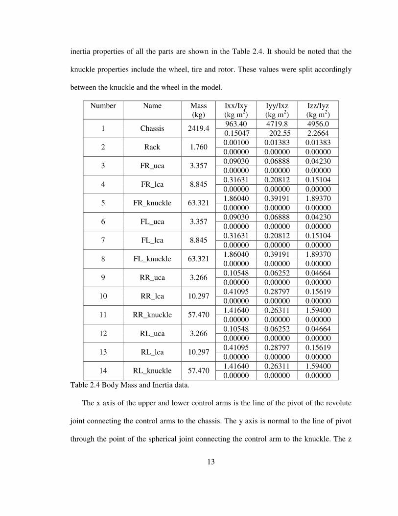
13
inertia properties of all the parts are shown in the Table 2.4. It should be noted that the
knuckle properties include the wheel, tire and rotor. These values were split accordingly
between the knuckle and the wheel in the model.
Number Name Mass (kg)
Ixx/Ixy (kg m2)
Iyy/Ixz (kg m2)
Izz/Iyz (kg m2)
963.40 4719.8 4956.0 1 Chassis 2419.4
0.15047 202.55 2.2664 0.00100 0.01383 0.01383
2 Rack 1.760 0.00000 0.00000 0.00000 0.09030 0.06888 0.04230
3 FR_uca 3.357 0.00000 0.00000 0.00000 0.31631 0.20812 0.15104
4 FR_lca 8.845 0.00000 0.00000 0.00000 1.86040 0.39191 1.89370
5 FR_knuckle 63.321 0.00000 0.00000 0.00000 0.09030 0.06888 0.04230
6 FL_uca 3.357 0.00000 0.00000 0.00000 0.31631 0.20812 0.15104
7 FL_lca 8.845 0.00000 0.00000 0.00000 1.86040 0.39191 1.89370
8 FL_knuckle 63.321 0.00000 0.00000 0.00000 0.10548 0.06252 0.04664
9 RR_uca 3.266 0.00000 0.00000 0.00000 0.41095 0.28797 0.15619
10 RR_lca 10.297 0.00000 0.00000 0.00000 1.41640 0.26311 1.59400
11 RR_knuckle 57.470 0.00000 0.00000 0.00000 0.10548 0.06252 0.04664
12 RL_uca 3.266 0.00000 0.00000 0.00000 0.41095 0.28797 0.15619
13 RL_lca 10.297 0.00000 0.00000 0.00000 1.41640 0.26311 1.59400
14 RL_knuckle 57.470 0.00000 0.00000 0.00000
Table 2.4 Body Mass and Inertia data.
The x axis of the upper and lower control arms is the line of the pivot of the revolute
joint connecting the control arms to the chassis. The y axis is normal to the line of pivot
through the point of the spherical joint connecting the control arm to the knuckle. The z

14
axis is then normal to each of these axes. The y axis of the knuckles is the rotation axis of
the wheel pointing to the right of the vehicle. The x axis is in the forward direction and
the z axis is downward. The x axis for the rack is along its direction of motion. The y and
z axes are arbitrarily chosen as normal to the x axis.
2.4 Springs and Shock Absorbers
The springs are modeled as nonlinear single component forces (S force in Adams)
acting between two points which are the mounting points of the strut. The force is defined
by a 2D curve with spring deflection on the x axis and force on the y axis. The spring
stiffness curves were calculated from the results of bounce tests performed by SEA, Ltd.
[5].
The shock absorbers are modeled as nonlinear single component forces acting
between the same points as the strut. The force is defined by a 2D curve with deformation
velocity along the x axis and force on the y axis. The front and rear shocks were tested at
Detroit Testing Laboratory, Inc. on a shock dynamometer. A curve fit was done on all the
data points for the various frequencies. This curve is used as the damping curve in the
model and the frequency dependence of the shock absorber is not modeled.
2.5 Tires and Road
The tires and road are modeled using the Adams Tire module available in Adams
View. One of the default flat road profiles available in the Adams database is used for the
road. The tire property file suitable for P264/70R17 113S tires was used.
15
2.6 Drive Train
The vehicle model is run only in coast mode for testing the ESC and CES systems,
and for this reason a drive train is not incorporated in the model. Instead, forced motions
are applied at the wheels to control the speed. The motions are then switched off using
scripted controls to let the vehicle coast while the maneuver is performed. Since the
scripted controls cannot be used during co-simulation with Matlab, torques are used
instead of the forced motions to control the vehicle speed when co-simulating with
Matlab.
2.7 Modeling Measures
Since Adams View is a general purpose multibody dynamics simulation software, it
does not have any specialized tools to measure the various vehicle parameters that need
to be monitored and recorded to compare the performance of the vehicle. Hence the
different tools to measure and monitor various parameters like steering angle, camber
angle, roll angle etc are created. Listed below are a few examples of these tools.
2.7.1 Wheel Camber Angle
The wheel camber angle is measured using two markers that are positioned on the
knuckle of the wheel. The first marker (steerangle_ref2) is situated at the wheel center on
the knuckle, and the second marker (steerangle_ref) is positioned on the axis of rotation
of the wheel but slightly inboard. The measure is defined in Adams as the equation:
)_refsteerangle_ref2,steerangle(
angle_ref)steer e_ref2,(steerangl
DY
DZATANSteerangle = (2.1)

16
DZ gives the z displacement and DY gives the y displacement between the two
markers specified with respect to the global origin. ATAN is the command for the inverse
tangent.
2.7.2 Front Wheel Steer Angle
The road wheel steer angle is calculated using the same markers used to measure the
camber angle. The steer angle measure is defined by the equation:
body.cm) _ref,steerangle gle_ref2,DY(steeran
body.cm) _ref,steerangle gle_ref2,DX(steeranATANSteer = (2.2)
The command DX is followed by the names of three markers, which returns the x
displacement between the first two markers with respect to the coordinate system of the
third marker (body.cm) which is the center of gravity of the chassis. This is done so that
the readings are consistent when the vehicle is moving.
2.7.3 Roll Angle
The chassis roll angle is calculated in a similar fashion to the camber angle and steer
angle using two markers. The two markers are fixed to the chassis of the vehicle, the first
marker (body.cm) is at the center of gravity of the body while the second marker
(roll_measure) is on the same horizontal plane but slightly to one side of the first marker.
The measure is defined by the equation:
).,.,_(
).,_(
cmbodycmbodymeasurerollDY
cmbodymeasurerollDZASINRollAngle = (2.3)
The ASIN command returns the inverse sine of the value supplied.

17
2.7.4 Accelerometer Readings
The CES system requires the vertical accelerations from three accelerometers that are
placed in specific points on a horizontal plane. The CES system uses these readings to
compute the roll angle, roll rate, pitch angle and pitch rate of the vehicle. These
accelerations are measured by placing three markers at the specified locations and then
measuring their z component of their acceleration. Figure 2.5 shows the measure dialogue
box.
Figure 2.5 Vertical Acceleration Measure of Accelerometer

18
CHAPTER 3:
VALIDATION
3.1 Introduction
In any computer model, the accuracy of the simulation relies on the accuracy of the
model and the vehicle parameters used to build the model. Hence the mode is checked
against experimental data to ensure that the data matches to confirm the accuracy of the
model. Different quasi-static tests and dynamic maneuvers are used to validate the model.
The experimental laboratory suspension characteristic data was collected by SEA, Ltd.
using their in-house Suspension Parameter Measurement Device (SPMD), reference
[5].The experimental field data was collected by NHTSA’s VRTC at the Transportation
Research Center (TRC), reference [5].
3.2 Quasi-Static Tests
Five different quasi-static tests are used to validate the model, namely: Front Bounce
Test, Rear Bounce Test, Front Roll Test, Rear Roll Test and Steering Ratio Test. These
tests validate the suspension parameters and the suspension kinematics of the vehicle.
3.2.1 Bounce Tests
In the bounce tests, a static load is applied to the chassis of the vehicle through a bar
attached to the frame. For several loads the steer angle and camber angle are measured

19
against the suspension deflection for both the front and rear axle. During the test, the
steering wheel is locked and the tires are positioned on free floating wheel-pad units so
that no lateral or longitudinal forces, or aligning moments would exist at the tires. This is
simulated in the model by setting the road friction to zero.
3.2.1.1 Front Bounce Test
Figures 3.1, 3.2 and 3.3 show the comparison between the experimental and
simulation data for the front bounce test.
Front Suspension Rate
-8000
-6000
-4000
-2000
0
2000
4000
6000
8000
-0.10 -0.05 0.00 0.05 0.10 0.15
Suspension Deflection (m)
Ve
rtic
al F
orc
e (
N)
Simulation Experimental
Figure 3.1 Front Suspension Spring Rate plot

20
Front Suspension Bounce Steer
-0.8
-0.6
-0.4
-0.2
0.0
0.2
0.4
0.6
0.8
-0.10 -0.05 0.00 0.05 0.10 0.15
Front Suspension Deflection (m)
Ste
er
An
gle
(d
eg
)
Simulation Experimental
Figure 3.2 Front Suspension Bounce Steer plot
Front Suspension Bounce Camber
-4.0
-3.0
-2.0
-1.0
0.0
1.0
-0.10 -0.05 0.00 0.05 0.10 0.15
Suspension Deflection (m)
Ca
mb
er
An
gle
(d
eg
)
Simulation Experimental
Figure 3.3 Front Suspension Bounce Camber plot
Reviewing the plots, it is clear that the model is very close to the experimental data
and confirms the accuracy of the front suspension parameters.
21
3.2.1.2 Rear Bounce Test
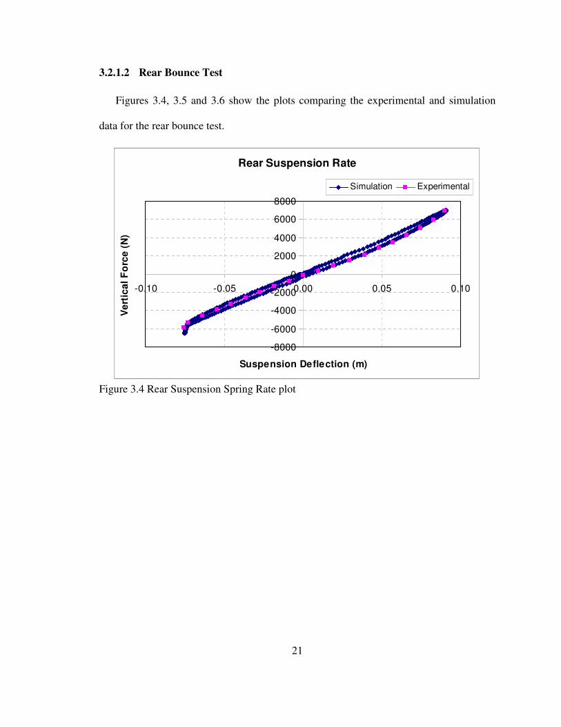
Figures 3.4, 3.5 and 3.6 show the plots comparing the experimental and simulation
data for the rear bounce test.
Rear Suspension Rate
-8000
-6000
-4000
-2000
0
2000
4000
6000
8000
-0.10 -0.05 0.00 0.05 0.10
Suspension Deflection (m)
Ve
rtic
al
Fo
rce
(N
)
Simulation Experimental
Figure 3.4 Rear Suspension Spring Rate plot

22
Rear Suspension Bounce Steer
-1.60
-1.20
-0.80
-0.40
0.00
0.40
-0.10 -0.05 0.00 0.05 0.10
Suspension Deflection (m)
Ste
er
An
gle
(d
eg
)
Simulation Experimental
Figure 3.5 Rear Suspension Bounce Steer plot
Rear Suspension Bounce Camber
-6.00
-4.00
-2.00
0.00
2.00
4.00
6.00
-0.10 -0.05 0.00 0.05 0.10
Suspension Deflection (m)
Ca
mb
er
An
gle
(d
eg
)
Simulation Experimental
Figure 3.6 Rear Suspension Bounce Camber plot
The simulation and experimental data match well for the rear spring rate plot while
some deviation is observed in the Rear Bounce Steer and Bounce Camber plots. Since the
magnitudes of the angles in question are very small, these deviations have only a

23
secondary effect on full vehicle response. These tests validate the rear suspension
parameters.
3.2.2 Roll Test
The roll test is performed by rolling the chassis of the vehicle with respect to the
wheels. The roll moment, camber angle and steer angles are measured against the roll
angle for both the front and rear axles. Similar to the bounce test, the wheels are placed
on free moving pads and the steering wheel is locked. This test serves to check the
accuracy of the roll stiffness bar and suspension kinematics.
3.2.2.1 Front Roll Test
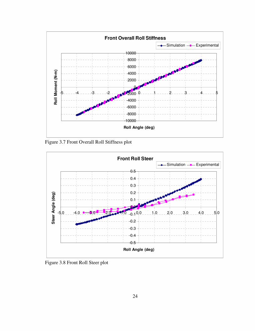
Figures 3.7, 3.8 and 3.9 show the comparison of experimental and simulation data for
the front roll test. Reviewing the plots, it is clear that the model very closely follows the
experimental results. A minor deviation is observed in the Roll Steer plot, but since it is
only to the order of a fraction of a degree, it can be neglected. This test confirms the
accuracy of the kinematics as well as the roll stiffness parameters of the front suspension.
24
Front Overall Roll Stiffness
-10000
-8000
-6000
-4000
-2000
0
2000
4000
6000
8000
10000
-5 -4 -3 -2 -1 0 1 2 3 4 5
Roll Angle (deg)
Ro
ll M
om
en
t (N
-m)
Simulation Experimental
Figure 3.7 Front Overall Roll Stiffness plot
Front Roll Steer
-0.5
-0.4
-0.3
-0.2
-0.1
0.0
0.1
0.2
0.3
0.4
0.5
-5.0 -4.0 -3.0 -2.0 -1.0 0.0 1.0 2.0 3.0 4.0 5.0
Roll Angle (deg)
Ste
er
An
gle
(d
eg
)
Simulation Experimental
Figure 3.8 Front Roll Steer plot
25
Front Roll Camber
-4.00
-3.00
-2.00
-1.00
0.00
1.00
2.00
3.00
4.00
-5.00 -4.00 -3.00 -2.00 -1.00 0.00 1.00 2.00 3.00 4.00 5.00
Roll Angle (deg)
Cam
ber
An
gle
(d
eg
)
Simulation Experimental
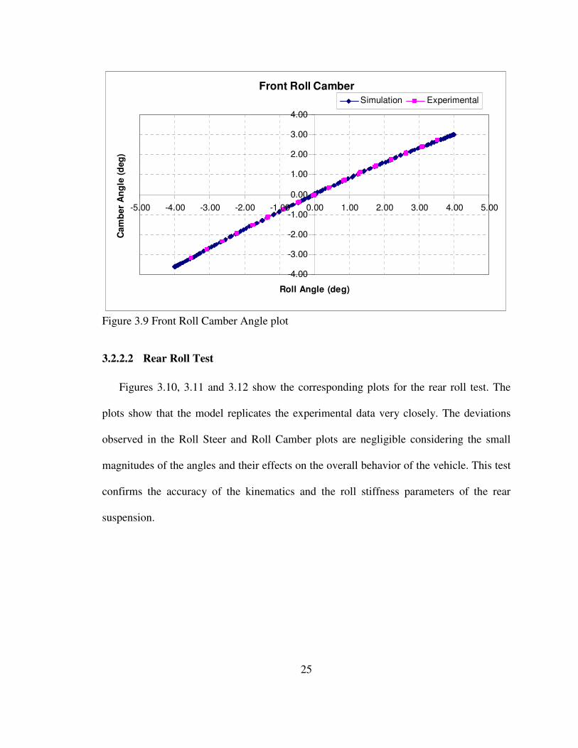
Figure 3.9 Front Roll Camber Angle plot
3.2.2.2 Rear Roll Test
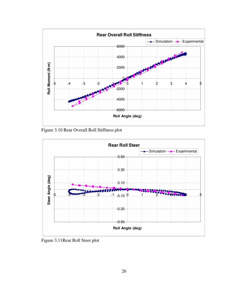
Figures 3.10, 3.11 and 3.12 show the corresponding plots for the rear roll test. The
plots show that the model replicates the experimental data very closely. The deviations
observed in the Roll Steer and Roll Camber plots are negligible considering the small
magnitudes of the angles and their effects on the overall behavior of the vehicle. This test
confirms the accuracy of the kinematics and the roll stiffness parameters of the rear
suspension.
26
Rear Overall Roll Stiffness
-6000
-4000
-2000
0
2000
4000
6000
-5 -4 -3 -2 -1 0 1 2 3 4 5
Roll Angle (deg)
Ro
ll M
om
en
t (N
-m)
Simulation Experimental
Figure 3.10 Rear Overall Roll Stiffness plot
Rear Roll Steer
-0.50
-0.30
-0.10
0.10
0.30
0.50
-5 -4 -3 -2 -1 0 1 2 3 4 5
Roll Angle (deg)
Ste
er
An
gle
(d
eg
)
Simulation Experimental
Figure 3.11Rear Roll Steer plot

27
Rear Roll Camber
-4
-3
-2
-1
0
1
2
3
4
-5 -4 -3 -2 -1 0 1 2 3 4 5
Roll Angle (deg)
Cam
ber
An
gle
(d
eg
)
Simulation Experimental
Figure 3.12 Rear Roll Camber plot
3.2.3 Steering Ratio Test
The steering ratio test is performed by rotating the hand steering wheel and measuring
the steer angle of the road wheel. This test is used to measure the ratio of hand wheel
angle to road wheel angle. Figure 3.13 shows the plot of hand wheel angle versus the
road wheel angle of the model. The steering wheel ratio from the plot 20.11 given by the
slope of the plot compares will with the experimental value of 19.71 from reference
[5].This test validates the steering system kinematics of the model.
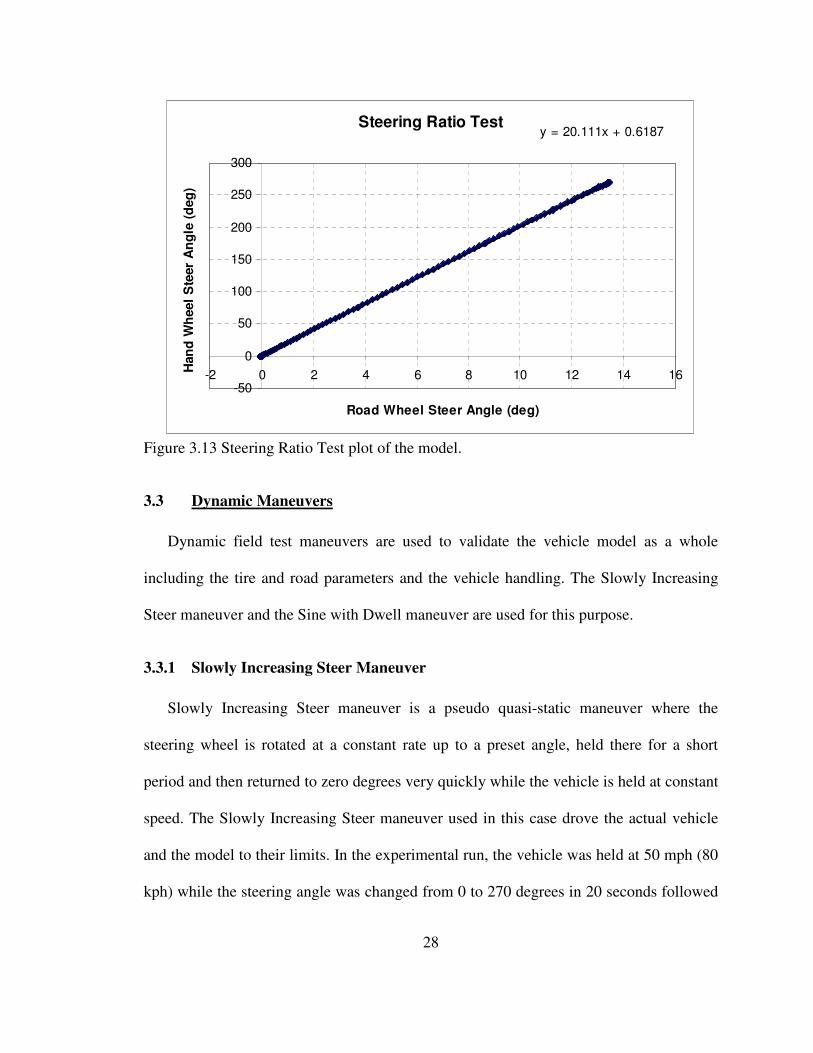
28
Steering Ratio Testy = 20.111x + 0.6187
-50
0
50
100
150
200
250
300
-2 0 2 4 6 8 10 12 14 16
Road Wheel Steer Angle (deg)
Han
d W
heel
Ste
er
An
gle
(d
eg
)
Figure 3.13 Steering Ratio Test plot of the model.
3.3 Dynamic Maneuvers
Dynamic field test maneuvers are used to validate the vehicle model as a whole
including the tire and road parameters and the vehicle handling. The Slowly Increasing
Steer maneuver and the Sine with Dwell maneuver are used for this purpose.
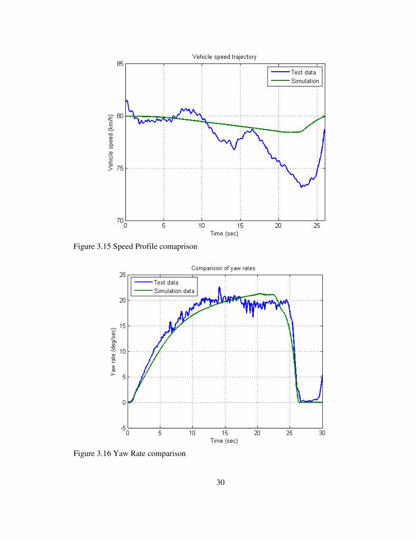
3.3.1 Slowly Increasing Steer Maneuver
Slowly Increasing Steer maneuver is a pseudo quasi-static maneuver where the
steering wheel is rotated at a constant rate up to a preset angle, held there for a short
period and then returned to zero degrees very quickly while the vehicle is held at constant
speed. The Slowly Increasing Steer maneuver used in this case drove the actual vehicle
and the model to their limits. In the experimental run, the vehicle was held at 50 mph (80
kph) while the steering angle was changed from 0 to 270 degrees in 20 seconds followed

29
by a dwell of 2 seconds and then brought back to 0 degrees in 4 seconds. The same
steering profile is used for the simulation runs to compare the plots. Figures 3.14 – 3.20
show the plots comparing the simulation and experimental results.
Figure 3.14 Steering Profile of Slowly Increasing Steer Maneuver
30
Figure 3.15 Speed Profile comaprison
Figure 3.16 Yaw Rate comparison
31
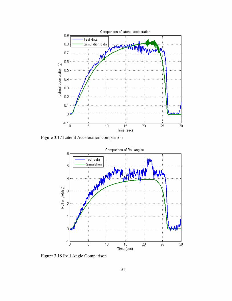
Figure 3.17 Lateral Acceleration comparison
Figure 3.18 Roll Angle Comparison

32
Figure 3.19 Roll Rate comparison
Figure 3.20 Pitch Rate comparison
33
Reviewing the plots, we can see that the Adams model replicates the experimental
data well. The maximum yaw rate and lateral accelerations match well, but the test
vehicle did not maintain full test speed beyond about 17 seconds. This reduction in test
speed resulted in reduced yaw rate and lateral acceleration responses between 17 and 22
seconds. The roll angle magnitudes are consistently lower than the experimental values,
but closely follow the same trends as do the other plots.
3.3.2 Sine with Dwell Maneuver
According to the Federal Motor Vehicle Safety Standards 126 (FMVSS 126) set by
the National Highway Transportation Safety Association (NHTSA), the Sine with Dwell
maneuver is the preferred maneuver to quantify the ESC effectiveness. Since the purpose
of this thesis is to study the effect of the CES shock absorber system on the performance
of the ESC, it is critical that the model gives accurate results for this maneuver.
In this maneuver, the vehicle is accelerated up to 50 mph (80 kph) and the throttle is
cut off to let it coast. As soon as the vehicle starts to coast down from the preset speed the
steering input is started. The steering input is in the form of a 0.7 Hz sinusoidal wave
with a 500 ms pause after the third quarter-cycle. The maneuver used in the experimental
runs is replicated in the model for various peak steering angles ranging from 80 degrees
to a maximum of 160 degrees and the results are compared in the Figures 3.21 to 3.26.
34
(a) (b)
(c) (d)
(e)
Figure 3.21 Steering profiles for a) 80, b) 100, c) 120, d) 140 and e) 160 deg.

35
(a) (b)
(c) (d)
(e)
Figure 3.22 Lateral Acceleration comparisons for a) 80, b) 100, c) 120, d) 140 and e) 160
degrees

36
(a) (b)
(c) (d)
(e)
Figure 3.23 Yaw Rate Comparison for a) 80, b) 100, c) 120, d) 140 and e) 160 degrees.
37
(a) (b)
(c) (d)
(e)
Figure 3.24 Speed Trajectory comparison plots for a) 80, b) 100, c) 120, d) 140 and e)
160 degrees.

38
From the figures plotted above, it is clear that the model generates very good
predictions for lateral acceleration and yaw rate for the Sine with Dwell maneuver. Figure
3.24 compares the speed trajectory between the simulation and the experimental data.
There seems to be large deviation in these graphs. This is in fact misleading as in the first
four cases, the test maneuver ends before 3.5 seconds when the yaw rate drops to zero.
Thus the experimental speed data after about 3.5 seconds is when the driver has taken
control of the vehicle and braked. This causes the speed difference to look large at the
end of 5 seconds, whereas in reality this data is not relevant for the test. Taking this into
consideration, it is clear that the model predicts the vehicle behavior very accurately.
Studying case (e) with 160 degrees steering, it is clear that both the experimental run
and the simulation yaw rates do not return to zero. This case is the “loss of control” run
for both simulation and experiment. This reiterates that the model is very well tuned to
correlate with experimental data.
Figures 3.25 below shows the roll angle plots for the five cases. Though the
simulation predicts the trends very well, the roll angle magnitudes are consistently lower
than the experimental values. This trend is consistent with that observed with the Slowly
Increasing Steer maneuver (Figure 3.18). Though the roll inertias have been modeled as
measured for the actual vehicle, this may be due to the fact that the actual vehicle has
more dynamic roll compliances, due to bushings etc., than measured on the SPMD and
that the real vehicle is not a perfect rigid body as it is in the model.
39
(a) (b)
(c) (d)
(e)
Figure 3.25 Roll Angle comparison plots for a) 80, b) 100, c) 120, d) 140 and e) 160
degrees.
40
(a) (b)
(c) (d)
(e)
Figure 3.26 Roll Rate comparison plots for a) 80, b) 100, c) 120, d) 140 and e) 160
degrees.

41
(a) (b)
(c) (d)
(e)
Figure 3.27 Pitch Rate Comparison Plots for a) 80, b) 100, c) 120, d) 140 and e) 160
degrees.
42
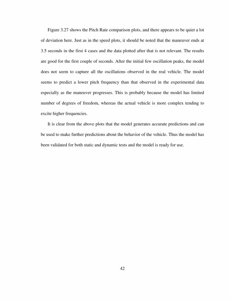
Figure 3.27 shows the Pitch Rate comparison plots, and there appears to be quiet a lot
of deviation here. Just as in the speed plots, it should be noted that the maneuver ends at
3.5 seconds in the first 4 cases and the data plotted after that is not relevant. The results
are good for the first couple of seconds. After the initial few oscillation peaks, the model
does not seem to capture all the oscillations observed in the real vehicle. The model
seems to predict a lower pitch frequency than that observed in the experimental data
especially as the maneuver progresses. This is probably because the model has limited
number of degrees of freedom, whereas the actual vehicle is more complex tending to
excite higher frequencies.
It is clear from the above plots that the model generates accurate predictions and can
be used to make further predictions about the behavior of the vehicle. Thus the model has
been validated for both static and dynamic tests and the model is ready for use.
43
CHAPTER 4:
CO-SIMULATION
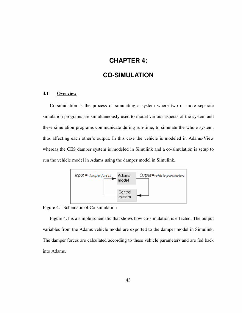
4.1 Overview
Co-simulation is the process of simulating a system where two or more separate
simulation programs are simultaneously used to model various aspects of the system and
these simulation programs communicate during run-time, to simulate the whole system,
thus affecting each other’s output. In this case the vehicle is modeled in Adams-View
whereas the CES damper system is modeled in Simulink and a co-simulation is setup to
run the vehicle model in Adams using the damper model in Simulink.
Figure 4.1 Schematic of Co-simulation
Figure 4.1 is a simple schematic that shows how co-simulation is effected. The output
variables from the Adams vehicle model are exported to the damper model in Simulink.
The damper forces are calculated according to these vehicle parameters and are fed back
into Adams.
44
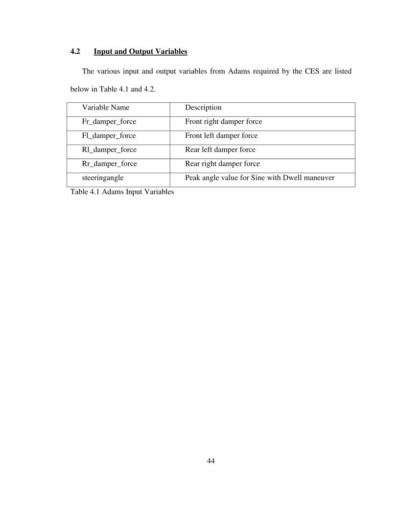
4.2 Input and Output Variables
The various input and output variables from Adams required by the CES are listed
below in Table 4.1 and 4.2.
Variable Name Description
Fr_damper_force Front right damper force
Fl_damper_force Front left damper force
Rl_damper_force Rear left damper force
Rr_damper_force Rear right damper force
steeringangle Peak angle value for Sine with Dwell maneuver
Table 4.1 Adams Input Variables

45
Variable Name Description
Az_S1 Vertical Accleration of sensor 1
Az_S2 Vertical Accleration of sensor 2
Az_S3 Vertical Accleration of sensor 3
Fl_damper_displacement Front left damper displacement
fr_damper_displacement Front right damper displacement
Rl_damper_displacement Rear left damper displacement
rr_damper_displacement Rear right damper displacement
Speed Vehicle speed
steeringangle Steering wheel angular displacement
steering_rate Steering wheel velocity
Brake_pressure Master cylinder pressure
Throttle Throttle position
Engine_torque Torque output at engine crank shaft
Engine_angular_speed Engine angular speed
Engine_angular_acc Engine angular acceleration
lateralaccleration Lateral Acceleration
Fl_damper_velocity Front left damper velocity
fr_damper_velocity Front right damper velocity
Rl_damper_velocity Rear left damper velocity
rr_damper_velocity Rear right damper velocity
Vz Vertical velocity of vehicle
Pitchrate Pitch Rate
Rollrate Roll Rate
Vertical_acc Vertical acceleration of chassis
Pitch_acc Pitch Acceleration
Roll_acc Roll Acceleration
Yawrate Yaw Rate
Rollangle Roll Angle
Table 4.2 Adams Output variables
46
4.3 Setting up the Co-simulation
The various steps involved in setting up a co-simulation between Adams and
Simulink are:
1. Loading Adams/Controls
2. Defining Input and Output Variables
3. Referencing Input Variables in the Adams Model
4. Exporting the Adams Block
5. Connecting the Adams Block and the CES Block in Simulink
6. Running the Co-simulation
7. Things to Remember
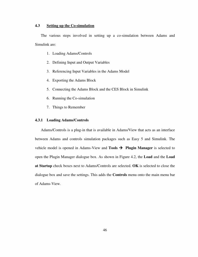
4.3.1 Loading Adams/Controls
Adams/Controls is a plug-in that is available in Adams/View that acts as an interface
between Adams and controls simulation packages such as Easy 5 and Simulink. The
vehicle model is opened in Adams-View and Tools ���� Plugin Manager is selected to
open the Plugin Manager dialogue box. As shown in Figure 4.2, the Load and the Load
at Startup check boxes next to Adams/Controls are selected. OK is selected to close the
dialogue box and save the settings. This adds the Controls menu onto the main menu bar
of Adams-View.

47
Figure 4.2 Plugin Manager to load Adams/Controls
4.3.2 Defining Input and Output Variables
Adams/Controls and controls applications such as Simulink communicate using what
are called as state variables. All input and output variables have to be defined as Adams
state variables. To create a new state variable, from the Build menu, System Element �
State Variable � New, is selected.

48
Figure 4.3 Create State Variable dialogue box for output variable
Figure 4.3 shows how output variables are defined, the name of the state variable is
entered in the Name box, and Run-Time Expression is selected in for the Definition box.
The expression to calculate the output variable is entered in the F(time,…) box.
As shown in Figure 4.4, input variables are also defined as state variables following
the same steps as for the output variables, except that the F(time,…) box is left with the
default value of zero. All the input and output variables, listed in Table 4.1 and 4.2, are
similarly defined.
Figure 4.4 Create State Variable dialogue box for input variable

49
4.3.3 Referencing Input Variables
Once the input and output variables have been defined, the input variable values that
are obtained from Simulink have to be applied/referenced at the proper location in the
Adams model. In this case, the value of the damper forces obtained from Simulink have
to be referenced at the respective damper s-forces. To reference the input variable,
Edit����Modify is selected. This opens the database navigator from which fr_damping is
double clicked. This opens the Modify Force dialogue box as shown in Figure 4.5.
Figure 4.5 Modify Force dialogue box
The Function box is filled in as VARVAL(fr_damper_force), where the command
VARVAL is used to reference the value of the input variable fr_damper_force as the
value to be used for the s-force fr_damping. The other input variables are also similarly
referenced at the corresponding s-forces and motions.
50
4.3.4 Exporting Adams block
Once the Input variables are referenced properly in Adams, the Adams model is ready
to be exported to Simulink as a control system block. To export the model,
Controls����Plant Export in selected which opens the Adams/Controls Plant Export
dialogue box, shown in Figure 4.6.
Figure 4.6 Adams Controls Plant Export dialogue box.
The input variables and output variables are listed in the order in which the respective
pins in the control block are to appear. It is important that the correct input and output
51
pins are connected to the correct control system elements for the proper functioning of
the system. For this reason the output variables are listed in the same order that the CES
controller reads them. Once the dialogue box is completed, OK is selected. This exports
three files with the file name specified in the File Prefix field of the dialogue box
followed by the extensions .adm, .cmd and .m. In this case the file name is specified as
Expedition_CES and thus the three files are Expedition_CES.adm, Expedition_CES.cmd
and Expedition_CES.m. These are saved in the working directory of Adams.
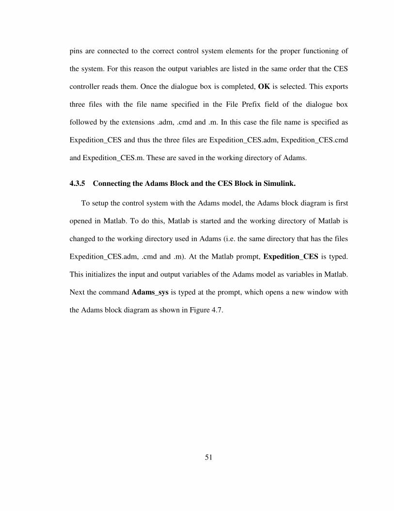
4.3.5 Connecting the Adams Block and the CES Block in Simulink.
To setup the control system with the Adams model, the Adams block diagram is first
opened in Matlab. To do this, Matlab is started and the working directory of Matlab is
changed to the working directory used in Adams (i.e. the same directory that has the files
Expedition_CES.adm, .cmd and .m). At the Matlab prompt, Expedition_CES is typed.
This initializes the input and output variables of the Adams model as variables in Matlab.
Next the command Adams_sys is typed at the prompt, which opens a new window with
the Adams block diagram as shown in Figure 4.7.
52
Figure 4.7 Adams Block Diagram in Simulink
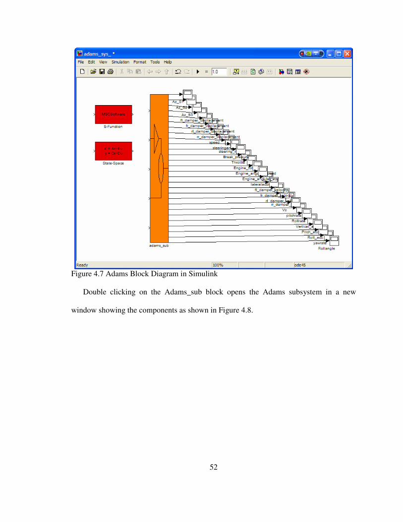
Double clicking on the Adams_sub block opens the Adams subsystem in a new
window showing the components as shown in Figure 4.8.
53
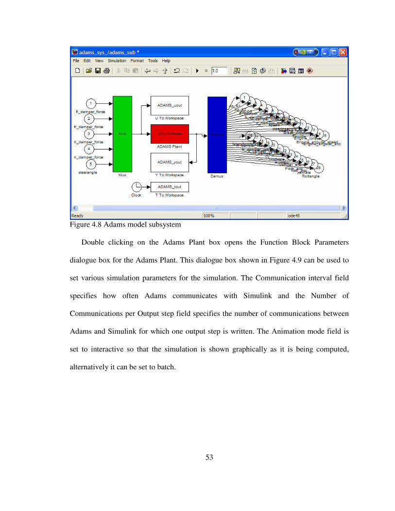
Figure 4.8 Adams model subsystem
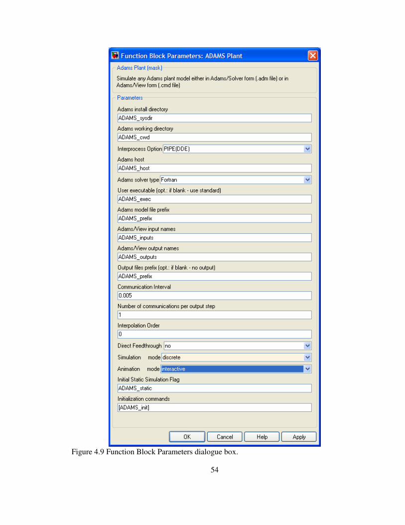
Double clicking on the Adams Plant box opens the Function Block Parameters
dialogue box for the Adams Plant. This dialogue box shown in Figure 4.9 can be used to
set various simulation parameters for the simulation. The Communication interval field
specifies how often Adams communicates with Simulink and the Number of
Communications per Output step field specifies the number of communications between
Adams and Simulink for which one output step is written. The Animation mode field is
set to interactive so that the simulation is shown graphically as it is being computed,
alternatively it can be set to batch.
54
Figure 4.9 Function Block Parameters dialogue box.

55
The Adams_sub block is then copied and pasted onto a new model window along
with the CES control system. The outputs from the Adams_sub block are then connected
to the inputs of the CES system and the outputs from the CES are fed back into the
Adams_sub block. Figure 4.10 shows the whole system.
Figure 4.10 Expedition with CES control diagram in Simulink.
4.3.6 Running the Co-simulation
Once the system is setup, the simulation time is entered in the box on top of the
screen and the play button is clicked to run the simulation. Simulink invokes Adams and
runs the model in Adams/View while the damper forces are calculated in Simulink and
fed into Adams while the simulation is running. Thus co-simulation is achieved.
56
4.3.7 Things to Remember
The variable ADAMS_cwd in the matlab file stands for Adams current working
directory, and stores the path of the current working directory that was in use when the
file was exported. This path has to match with the directory in which the Adams files are
when they are run. Thus if the files are moved, or the directory name changed, the
ADAMS_cwd variable has to be accordingly updated.
Adams Host name: The Adams Host Name field in the Adams Controls Plant Export
dialogue box (Figure 4.6) specifies the name of the computer along with the network
path. This information is stored in the variable ADAMS_host in the matlab file. This
information changes from computer to computer and from network to network. Thus this
file can only be run from the computer it was first exported from while it is connected to
the same network as it was when it was exported. To run from another system, all the
files have to be copied to the new system and the value of the ADAMS_host variable has
to be changed to match that of the new system, also the ADAMS_cwd variable has to be
updated to match the path in the new system.
57
CHAPTER 5:
ELECTRONIC STABILITY CONTROL
5.1 Overview
Electronic stability control (ESC) systems are active control systems that act to
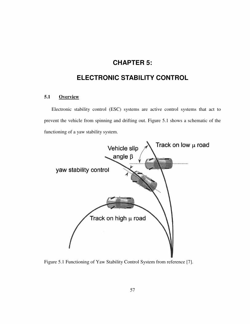
prevent the vehicle from spinning and drifting out. Figure 5.1 shows a schematic of the
functioning of a yaw stability system.
Figure 5.1 Functioning of Yaw Stability Control System from reference [7].

58
In the figure, the lower curve shows the trajectory the vehicle should follow in
response to a steering input from the driver if the road were dry and had a high tire road
friction coefficient. In this case, the high friction is able to provide sufficient lateral
forces to the car to negotiate the curved road. If the coefficient of friction of the road was
low or if the vehicle was traveling too fast, the vehicle would be unable to follow the
same curvature, but instead follow a wider curve like the one depicted by the upper curve
of Figure 5.1. The function of the ESC is to restore the yaw velocity of the vehicle as
much as possible to the nominal motion expected by the driver. If the friction is too low,
the ESC may not be able to entirely achieve the nominal yaw rate that is expected on a
high friction surface. In this case the ESC would partially succeed by making the yaw
rate as close to the nominal rate as possible as shown by the middle curve in Figure 5.1.
(From reference [7])
The active control can be effected in different ways, either by active torque
distribution, where the power delivered to each wheel is controlled to achieve the yaw
rate or by steer-by-wire where steering corrections are given by the computer to
compensate for the yaw rate. The Expedition uses a differential braking ESC system,
where the brakes on each wheel are individually applied to correct the yaw rate and
heading of the vehicle.
5.2 ESC Model
The ESC system used with the Adams model is modeled in Matlab Simulink. It is a
modified version of the ESC system used with the CarSim Expedition model developed
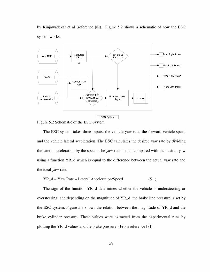
59
by Kinjawadekar et al (reference [8]). Figure 5.2 shows a schematic of how the ESC
system works.
Figure 5.2 Schematic of the ESC System
The ESC system takes three inputs; the vehicle yaw rate, the forward vehicle speed
and the vehicle lateral acceleration. The ESC calculates the desired yaw rate by dividing
the lateral acceleration by the speed. The yaw rate is then compared with the desired yaw
using a function YR_d which is equal to the difference between the actual yaw rate and
the ideal yaw rate.
YR_d = Yaw Rate – Lateral Acceleration/Speed (5.1)
The sign of the function YR_d determines whether the vehicle is understeering or
oversteering, and depending on the magnitude of YR_d, the brake line pressure is set by
the ESC system. Figure 5.3 shows the relation between the magnitude of YR_d and the
brake cylinder pressure. These values were extracted from the experimental runs by
plotting the YR_d values and the brake pressure. (From reference [8]).
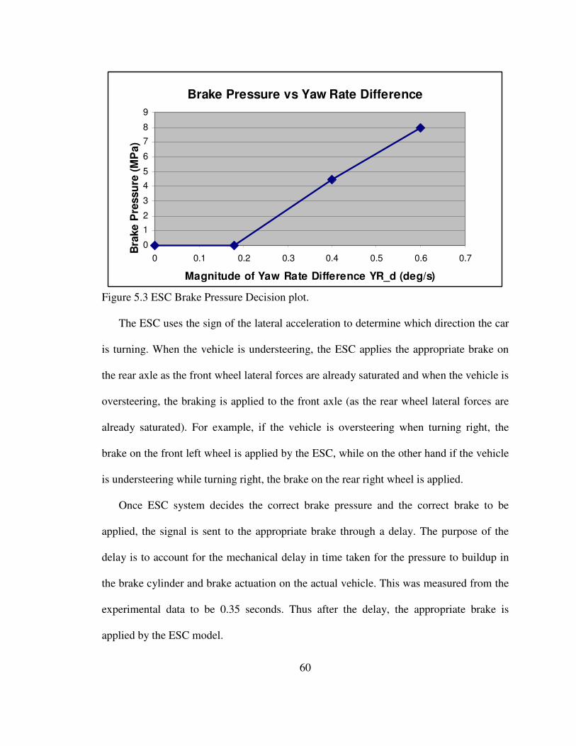
60
Brake Pressure vs Yaw Rate Difference
0
1
2
3
4
5
6
7
8
9
0 0.1 0.2 0.3 0.4 0.5 0.6 0.7
Magnitude of Yaw Rate Difference YR_d (deg/s)
Bra
ke P
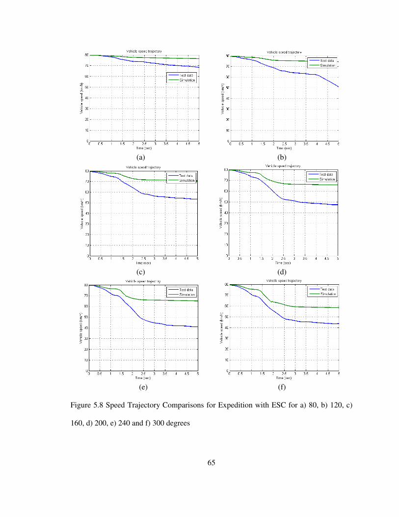
ressu
re (
MP
a)
Figure 5.3 ESC Brake Pressure Decision plot.
The ESC uses the sign of the lateral acceleration to determine which direction the car
is turning. When the vehicle is understeering, the ESC applies the appropriate brake on
the rear axle as the front wheel lateral forces are already saturated and when the vehicle is
oversteering, the braking is applied to the front axle (as the rear wheel lateral forces are
already saturated). For example, if the vehicle is oversteering when turning right, the
brake on the front left wheel is applied by the ESC, while on the other hand if the vehicle
is understeering while turning right, the brake on the rear right wheel is applied.
Once ESC system decides the correct brake pressure and the correct brake to be
applied, the signal is sent to the appropriate brake through a delay. The purpose of the
delay is to account for the mechanical delay in time taken for the pressure to buildup in
the brake cylinder and brake actuation on the actual vehicle. This was measured from the
experimental data to be 0.35 seconds. Thus after the delay, the appropriate brake is
applied by the ESC model.
61
5.3 Validation
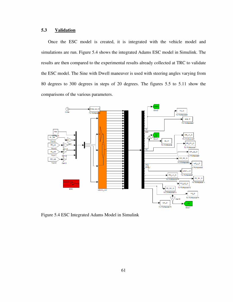
Once the ESC model is created, it is integrated with the vehicle model and
simulations are run. Figure 5.4 shows the integrated Adams ESC model in Simulink. The
results are then compared to the experimental results already collected at TRC to validate
the ESC model. The Sine with Dwell maneuver is used with steering angles varying from
80 degrees to 300 degrees in steps of 20 degrees. The figures 5.5 to 5.11 show the
comparisons of the various parameters.
Figure 5.4 ESC Integrated Adams Model in Simulink

62
(a) (b)
(c) (d)
(e) (f)
Figure 5.5 Steering Profiles for Expedition with ESC for a) 80, b) 120, c) 160, d) 200, e)
240 and f) 300 degrees
63
(a) (b)
(c) (d)
(d) (e)
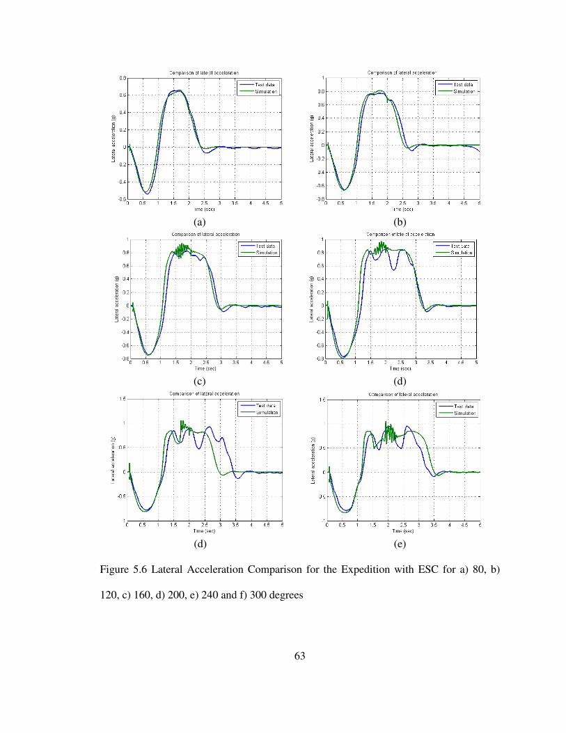
Figure 5.6 Lateral Acceleration Comparison for the Expedition with ESC for a) 80, b)
120, c) 160, d) 200, e) 240 and f) 300 degrees
64
(a) (b)
(c) (d)
(e) (f)
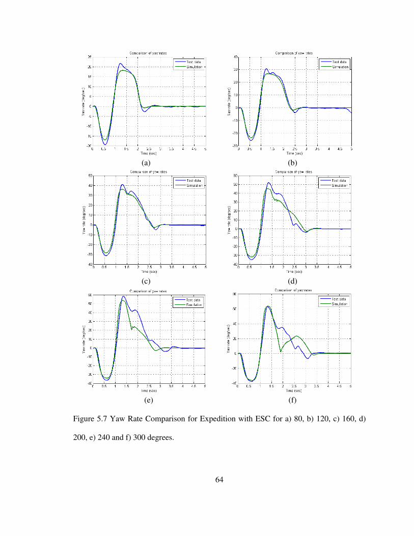
Figure 5.7 Yaw Rate Comparison for Expedition with ESC for a) 80, b) 120, c) 160, d)
200, e) 240 and f) 300 degrees.
65
(a) (b)
(c) (d)
(e) (f)
Figure 5.8 Speed Trajectory Comparisons for Expedition with ESC for a) 80, b) 120, c)
160, d) 200, e) 240 and f) 300 degrees
66
(a) (b)
(c) (d)
(e) (f)
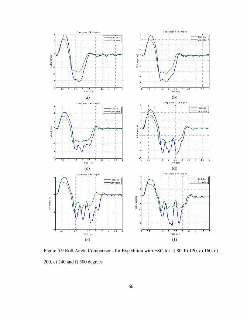
Figure 5.9 Roll Angle Comparisons for Expedition with ESC for a) 80, b) 120, c) 160, d)
200, e) 240 and f) 300 degrees

67
(a) (b)
(c) (d)
(e) (f)
Figure 5.10 Roll Rate Comparison for Expedition with ESC for a) 80, b) 120, c) 160, d)
200, e) 240 and f) 300 degrees

68
(a) (b)
(c) (d)
(e) (f)
Figure 5.11 Pitch Rate Comparison of Expedition with ESC for a) 80, b) 120, c) 160, d)
200, e) 240 and f) 300 degrees

69
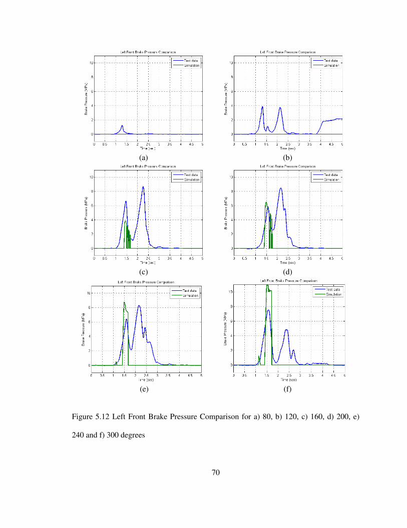
From the above graphs it is clear that the ESC model works very much like the actual
ESC for up to the 240 degree Sine with Dwell maneuver after which the results start to
deteriorate. Figure 5.6 shows lateral acceleration comparison, and there appears to be
some noise in the simulation data at around 1.5 seconds into the maneuver. This is in fact
not noise, but fluctuations caused due to rapid brake pulses that are applied at the same
time (Figure 5.12) during the simulation. Figure 5.9 shows the comparison of the roll
angles. The roll angles predicted are lower than that of the actual vehicle, which is
consistent with the previous roll angle predictions by the simulation.
To check the working of the ESC model, the brake pulses of the simulation and the
experimental runs are compared in Figures 5.12 and 5.13. These figures show the brake
pressures of the front left and front right brakes respectively. The rear brake pressures
remain zero for the experimental runs, as in this maneuver the vehicle is always
oversteering and hence the ESC activates the brakes only on the front axle. However in
the simulation the rear right wheel brake is activated for steering angles greater than 240
degrees. The brake pressure plot of the rear right wheel for the 300 degree Sine with
Dwell is shown in Figure 5.14.
70
(a) (b)
(c) (d)
(e) (f)
Figure 5.12 Left Front Brake Pressure Comparison for a) 80, b) 120, c) 160, d) 200, e)
240 and f) 300 degrees

71
(a) (b)
(c) (d)
(e) (f)
Figure 5.13 Right Front Brake Pressure Comparison for a) 80, b) 120, c) 160, d) 200, e)
240 and f) 300 degrees

72
Figure 5.14 Rear Right Brake Pressure plot for 300 deg Sine with Dwell Maneuver
From the above plots it is clear that the simulation needs much less ESC interference
than the actual vehicle to regain control. The front left brake plots indicate that the
simulation needs only one brake pulse around 1.5 seconds into the maneuver whereas the
actual vehicle has two brake pulses. A similar trend is observed for the front right brake
where the pulses in the simulation are of much less magnitude than observed on the
vehicle. Also from Figure 5.14, it is clear that the simulation vehicle starts to understeer
at around 2 seconds into the maneuver for runs with steering wheel angle greater than
240 degrees. However, the ESC model effectively brings the vehicle back to stability and
works well for most of the steering angles and can be used as a basis to quantify the
benefits of using the CES system.
73
CHAPTER 6:
CONTINUOUSLY CONTROLLED ELECTRONIC
SUSPENSION (CES) SYSTEM
6.1 Introduction
The CES system is an electronic suspension system that continuously adjusts shock-
absorber damping levels dependent on multiple driving variables, including driver inputs,
road conditions, and vehicle dynamics such as speed and cornering. The semi-active
system is able to achieve a balance between comfort and handling through the constantly
adaptive shock-absorber damping levels [9]. This system was developed by Tenneco
Automotive and the valve technology used was developed together with Öhlins Racing.
At the heart of the CES system is an electronic control unit (ECU) that processes
driver inputs and data from sensors placed at key locations on the vehicle. The sensors
include three accelerometers mounted on the vehicle body and four suspension position
sensors. The suspension position sensors give the current position of each strut on the car.
The ECU utilizes this information and sends signals that adjust independently the
damping level of each shock absorber valve in real time. Electronic dampers allow a
large range between maximum and minimum damping levels and adjust instantaneously
to ensure ride comfort and firm vehicle control [10].
74
The CES algorithm is programmed using Matlab Simulink, and a co-simulation is
setup with the ADAMS vehicle model to simulate a vehicle equipped with the CES
system.
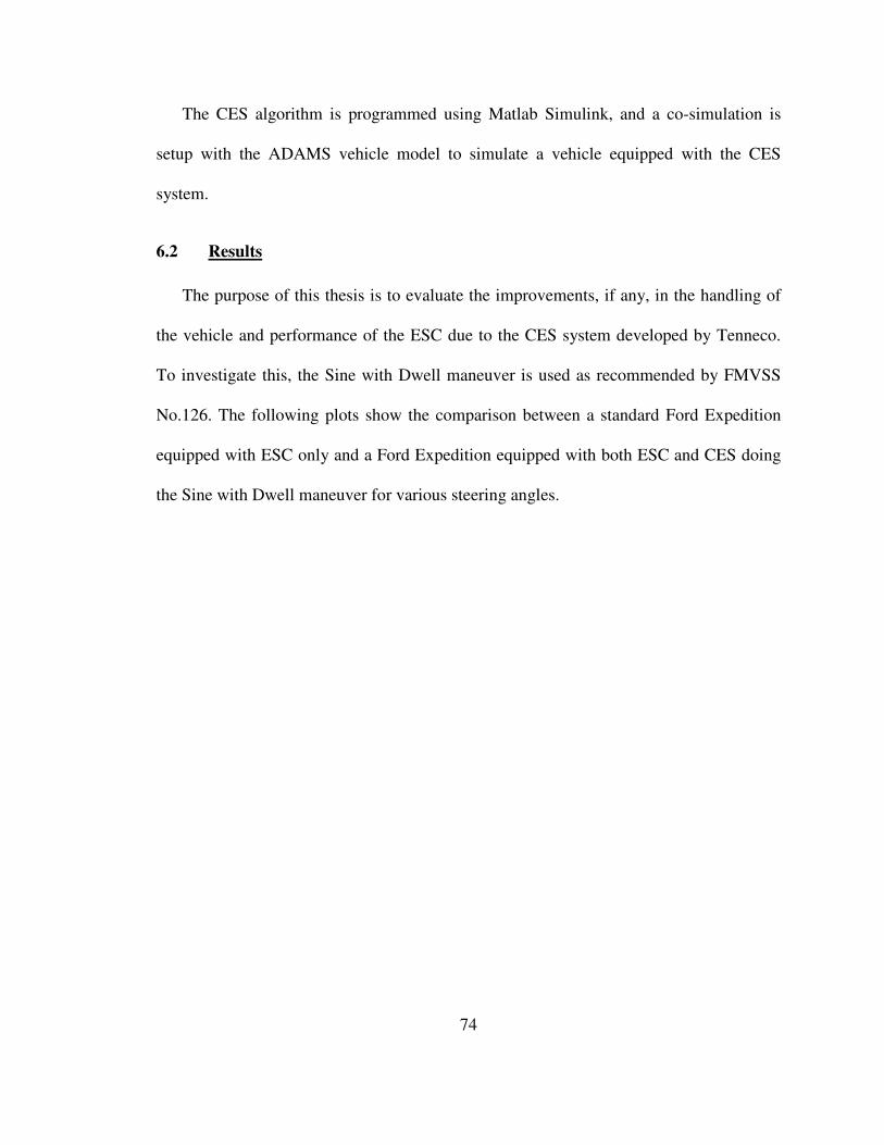
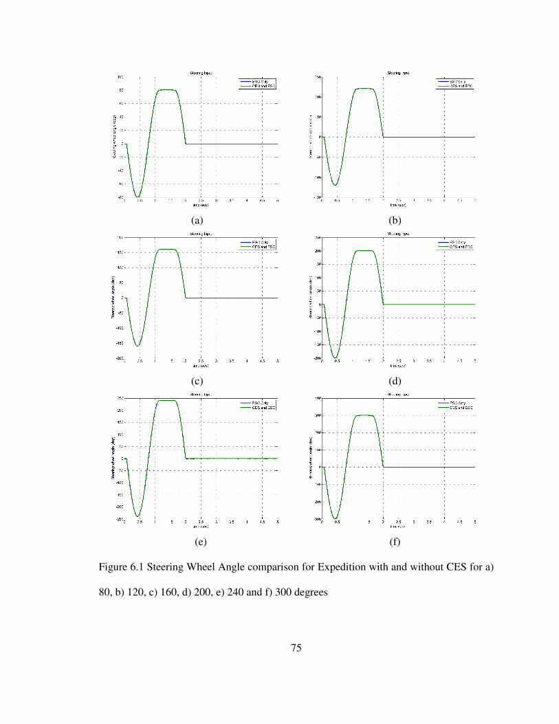
6.2 Results
The purpose of this thesis is to evaluate the improvements, if any, in the handling of
the vehicle and performance of the ESC due to the CES system developed by Tenneco.
To investigate this, the Sine with Dwell maneuver is used as recommended by FMVSS
No.126. The following plots show the comparison between a standard Ford Expedition
equipped with ESC only and a Ford Expedition equipped with both ESC and CES doing
the Sine with Dwell maneuver for various steering angles.
75
(a) (b)
(c) (d)
(e) (f)
Figure 6.1 Steering Wheel Angle comparison for Expedition with and without CES for a)
80, b) 120, c) 160, d) 200, e) 240 and f) 300 degrees
76
(a) (b)
(c) (d)
(e) (f)
Figure 6.2 Lateral Acceleration comparison for Expedition with and without CES for a)
80, b) 120, c) 160, d) 200, e) 240 and f) 300 degrees

77
(a) (b)
(c) (d)
(e) (f)
Figure 6.3 Yaw Rate Comparison for Expedition with and without CES for a) 80, b) 120,
c) 160, d) 200, e) 240 and f) 300 degrees

78
(a) (b)
(c) (d)
(e) (f)
Figure 6.4 Speed Trajectory comparison for Expedition with and without CES for a) 80,
b) 120, c) 160, d) 200, e) 240 and f) 300 degrees

79
(a) (b)
(c) (d)
(e) (f)
Figure 6.5 Roll Angle Comparison for Expedition with and without CES for a) 80, b)
120, c) 160, d) 200, e) 240 and f) 300 degrees
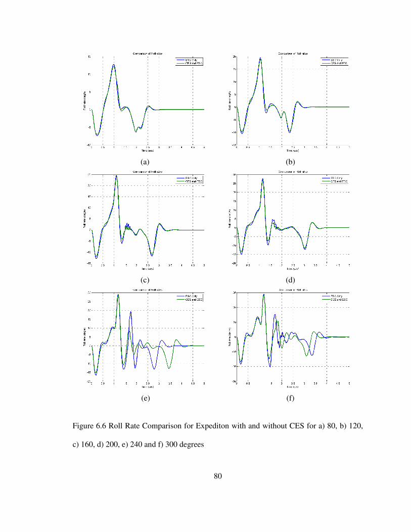
80
(a) (b)
(c) (d)
(e) (f)
Figure 6.6 Roll Rate Comparison for Expediton with and without CES for a) 80, b) 120,
c) 160, d) 200, e) 240 and f) 300 degrees
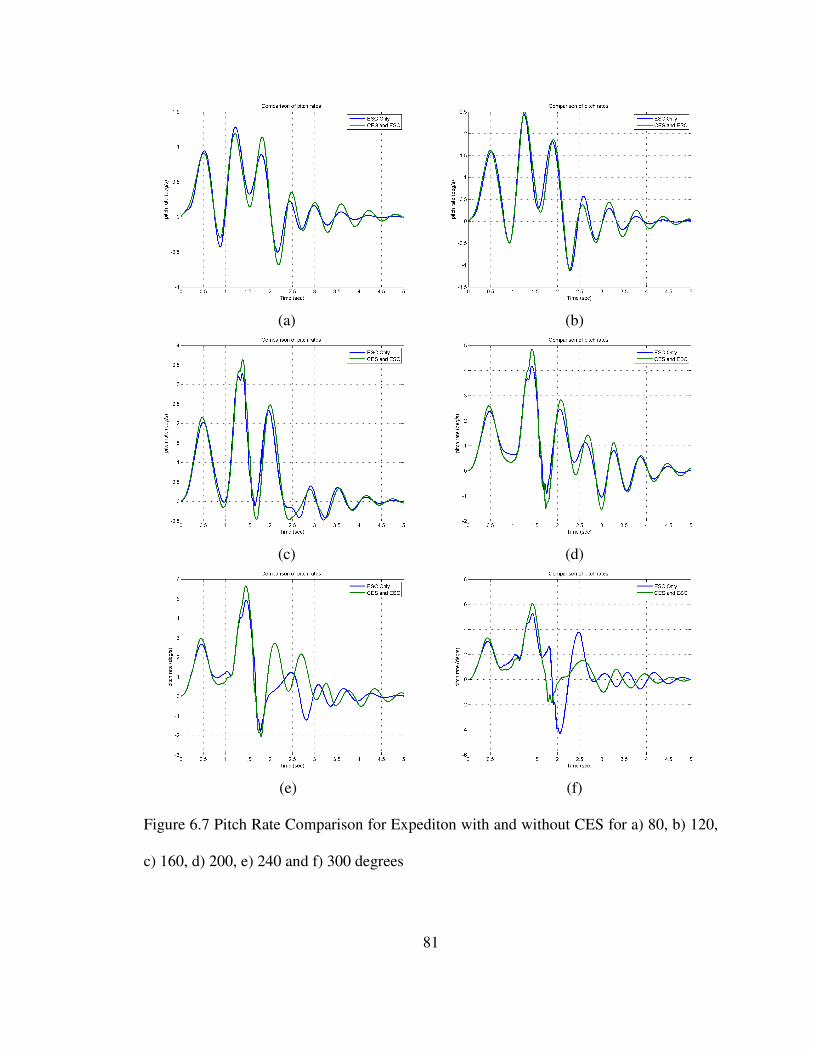
81
(a) (b)
(c) (d)
(e) (f)
Figure 6.7 Pitch Rate Comparison for Expediton with and without CES for a) 80, b) 120,
c) 160, d) 200, e) 240 and f) 300 degrees
82
Figure 6.8 shows the comparison of the right front and right rear damper
characteristics between the standard vehicle and the vehicle equipped with CES. These
plots show the dynamically changing characteristics of the CES dampers. The CES
dampers are also able to offer much higher damping forces compared to the stock
dampers. Figure 6.9 shows the damper forces versus time plots for both the vehicles. The
differences in peak forces produced by the stock and CES dampers are illustrated in this
plot.
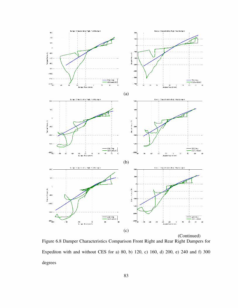
83
(a)
(b)
(c)
(Continued) Figure 6.8 Damper Characteristics Comparison Front Right and Rear Right Dampers for
Expediton with and without CES for a) 80, b) 120, c) 160, d) 200, e) 240 and f) 300
degrees
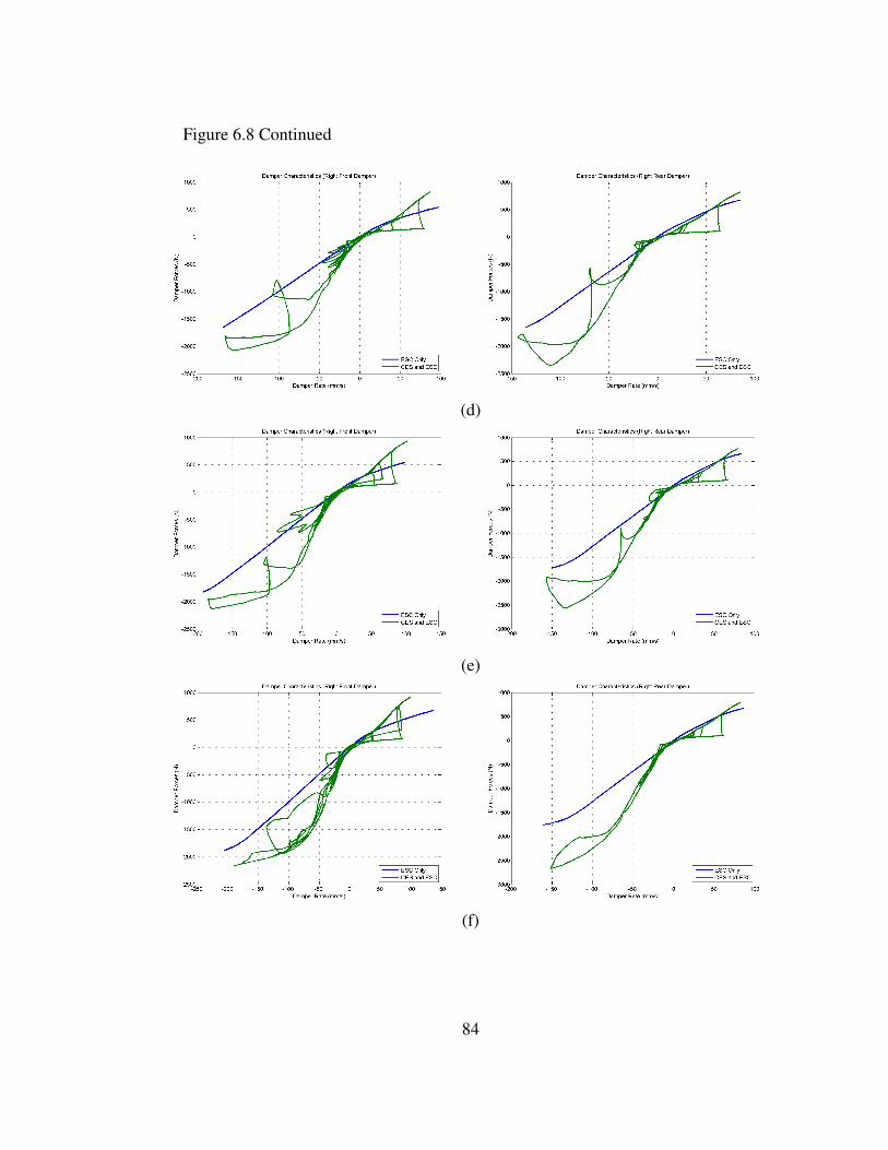
84
Figure 6.8 Continued
(d)
(e)
(f)

85
(a)
(b)
(c)
(Continued) Figure 6.9 Damper Forces Comparison for Expediton with and without CES for a) 80, b)
120, c) 160, d) 200, e) 240 and f) 300 degrees
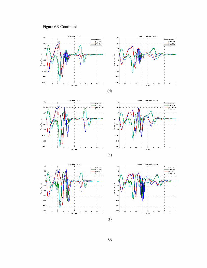
86
Figure 6.9 Continued
(d)
(e)
(f)
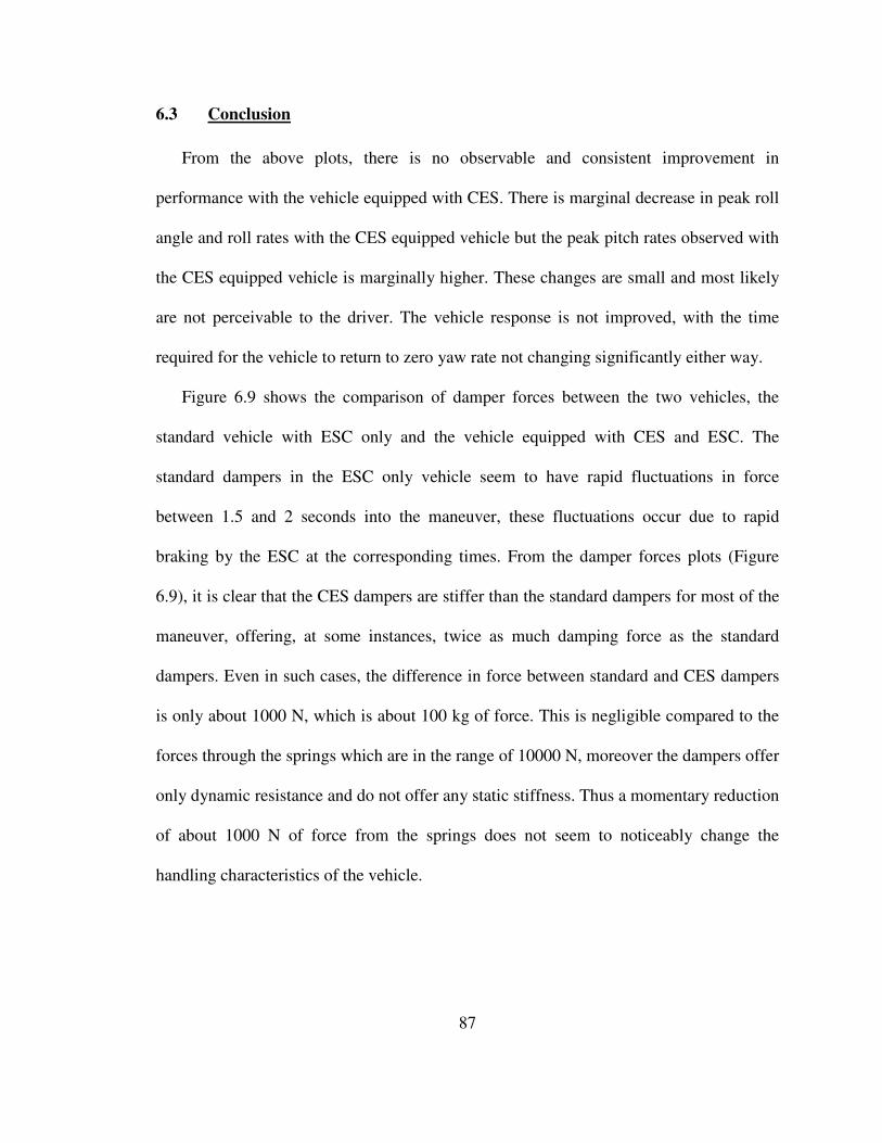
87
6.3 Conclusion
From the above plots, there is no observable and consistent improvement in
performance with the vehicle equipped with CES. There is marginal decrease in peak roll
angle and roll rates with the CES equipped vehicle but the peak pitch rates observed with
the CES equipped vehicle is marginally higher. These changes are small and most likely
are not perceivable to the driver. The vehicle response is not improved, with the time
required for the vehicle to return to zero yaw rate not changing significantly either way.
Figure 6.9 shows the comparison of damper forces between the two vehicles, the
standard vehicle with ESC only and the vehicle equipped with CES and ESC. The
standard dampers in the ESC only vehicle seem to have rapid fluctuations in force
between 1.5 and 2 seconds into the maneuver, these fluctuations occur due to rapid
braking by the ESC at the corresponding times. From the damper forces plots (Figure
6.9), it is clear that the CES dampers are stiffer than the standard dampers for most of the
maneuver, offering, at some instances, twice as much damping force as the standard
dampers. Even in such cases, the difference in force between standard and CES dampers
is only about 1000 N, which is about 100 kg of force. This is negligible compared to the
forces through the springs which are in the range of 10000 N, moreover the dampers offer
only dynamic resistance and do not offer any static stiffness. Thus a momentary reduction
of about 1000 N of force from the springs does not seem to noticeably change the
handling characteristics of the vehicle.

88
CHAPTER 7:
CONCLUSIONS AND RECOMMENDATIONS
7.1 Conclusions
In an effort to evaluate the benefits of the CES system, a model of the 2003 Ford
Expedition was created in Adams View. The various parameters of the model were
validated using quasi static tests results collected by SEA, Ltd. [5] and the overall
dynamics of the model was validated using experimental maneuvers [5]. From the
simulation, the model was shown to give accurate results for the purposes of this study.
Once the model was created, the ESC model was developed in Matlab Simulink and a
co-simulation was set up to integrate the ESC model with the vehicle model. The ESC
equipped vehicle model was validated using test data, and the ESC model proved to be
accurate for Sine with Dwell maneuvers of steering wheel angles up to 240 degrees. For
higher steering wheel angles, the results are still indicative of the performance of the test
vehicle but they start to deteriorate. Overall, the ESC model effectively reduces the time
required for the vehicle model to return to zero yaw rate in the Sine with Dwell
maneuver, and the results are similar to the ESC equipped test vehicle.
Next, a co-simulation was set up to incorporate the CES model, also programmed in
Matlab Simlink, into the vehicle model. Simulations were run and results were compared
with the results from the standard ESC equipped vehicle model. From the simulations,
89
the CES equipped vehicle was shown to offer no noticeable improvement in returning the
yaw rate to zero or in significantly reducing the roll and pitch response in the Sine with
Dwell maneuver. The CES system may offer comfort and customizability to the driver,
and may even improve handling under certain circumstances, but the results of this study
show that the CES system does not improve the performance of a vehicle put through the
Sine with Dwell maneuver.
7.2 Recommendations
It would be advisable to experimentally test a CES equipped vehicle and compare the
results with the simulation. Though simulation results are preferred as an initial
indication of trends, there is no substitute for actual testing. Testing would completely
validate the advantages, if any; of the system and also help ensure that the CES model
gives damper force outputs similar to the actual physical CES system.
The current Adams model provides very accurate results for the needs of this study,
but to further increase the scope of this model, there are several improvements that need
to be made. The tire model with the current tire parameters needs to be replaced with a
better tire model that reflects the properties of the actual tires more accurately.
The compliances added to the steering system of the model were values estimated
using scientific “guess-check” techniques. Though the model is providing accurate
results, it is possible that the compliances do not reflect the real values. The model does
not contain any other suspension compliance as all other joints are modeled as ideal
joints. Omitting the compliances can also lead to erroneous results. The suspension

90
characteristics could be better modeled to reflect the suspension compliances from test
data already available.
The ESC model created for this study is a very basic one, using the very basic inputs
and a simple algorithm. There is a lot of room to improve the ESC model. The algorithm
can be improved to take in more inputs such as steering rate. Other improvements would
include implementing an ABS and a roll stability system.
Lastly, a more detailed study of the effects of damping on ESC performance needs to
be done so that the CES algorithm can be improved. To achieve this, it would be ideal to
perform a full scale vehicle test and simulation using different damper settings and
comparing the results. With these changes/additions, one would have a better model and
a better understanding of the advantages of the CES system.
91
REFERENCES
1. U.S. Department of Transportation, NHTSA, “Traffic Safety Facts 2004”, 2004, DOT HS 809919
2. U.S. Department of Transportation, NHTSA, “PROPOSED FMVSS No.126 Electronic Stability Control Systems”, August 2006
3. Dang, Jennifer N., “Preliminary Results Analyzing The Effectiveness of Electronic Stability Control (ESC) Systems” September 2004, DOT HS809790
4. Forkenbrock, Garrick J., Elsasser, Devin., O’Harra, Bryan., “NHTSA’s Light Vehicle Handling and ESC Effectiveness Research Program” 05-0221
5. Pan, W. and Papelis, Y.E., “Real-Time Dynamic Simulation Of Vehicles With Electronic Stability Control: Modeling And Validation,” Int. J. Vehicle Systems Modeling and Testing, Vol. 1, Nos. 1/2/3, 2005
6. MSC Software Corp., “Getting Started Using Adams/Controls Introducing and Starting the Tutorials”, Mechanical Dynamics Inc., 2002
7. Rajamani, Rajesh “Vehicle Dynamics and Control”, Springer 2005
8. Kinjawadekar, T., Dixit, N. Heydinger, G.J., Guenther, D.A., and Salaani, M.K., “Vehicle Dynamics Modeling and Validation the 2003 Ford Expedition with ESC using CarSim”, SAE Paper 2009-01-0452, April 2008
9. http://www.trucktrend.com/features/news/2008/163_news080811_tenneco_will_p
rovide_ces_shock_absorbers_for_2009_volvo_xc60/index.html
10. http://www.tenneco.com/news/press/archive/press_2007/05082007.html