The Pennsylvania State University

The Graduate School

Department of Electrical Engineering

VECTOR SYMBOL DECODING WITH LISTS OF ALTERNATIVE VECTOR

SYMBOL CHOICES AND OUTER CONVOLUTIONAL CODES

A Thesis in

Electrical Engineering

by

Usana Tuntoolavest

Submitted in Partial Fulfillment of the Requirements

for the Degree of

Doctor of Philosophy

May 2002

We approve the thesis of Usana Tuntoolavest.

Date of Signature

John J. Metzner Professor of Electrical Engineering Professor of Computer Science and Engineering Thesis Advisor Chair of Committee

Mohsen Kavehrad Professor of Electrical Engineering

David J. Miller Associate Professor of Electrical Engineering

George Kesidis Associate Professor of Electrical Engineering

Associate Professor of Computer Science and Engineering

Guohong Cao Assistant Professor of Computer Science and Engineering

Kenneth Jenkins Professor of Electrical Engineering Head of the department of Electrical Engineering

ABSTRACT

Error correcting codes can play a key role in improving the efficiency and

reliability of digital communications. One way to simplify the decoder is by using

concatenated codes. Reed-Solomon codes have been popular as an outer code of

concatenated codes because they provide maximum minimum-distance (dmin) between

code words. However, Vector Symbol Decoding (VSD) for block outer codes has been

shown to achieve, in many cases, a better decoding success probability than Reed-

Solomon code decoding.

In this thesis, we present Vector Symbol Decoding (VSD) with list of alternative

vector symbol choices as a relatively simple and high performance decoding technique

for convolutional outer codes. The convolutional VSD technique has the advantage over

the block VSD technique in that most corrections are almost immediate based on

observation of only one or a few syndromes. (Some error events require consideration of

significantly larger numbers of syndromes, however.) The list decoding also improves the

performance and often simplifies the decoding. To implement VSD, the knowledge of the

parity check matrix is essential. A method for computing the parity check matrix for (n-

1)/n nonsystematic convolutional codes is presented. One main assumption of VSD is

that the error symbols are linearly independent, which usually is true for large symbol

size (24-bit, 32-bit or more). The effect of symbol size on the performance of VSD is

investigated and a way to reduce the decoding failures for smaller symbol size (16-bit) is

described.

iv

The performance of VSD is compared to the Reed-Solomon code decoding for

various types of inner codes and channel conditions. One difficulty in the comparison is

that VSD usually deals with a much larger vector symbol size than the Reed-Solomon

code decoding. In practice, Reed-Solomon codes are interleaved to handle larger symbol

size; thus, interleaved Reed-Solomon codes are also considered. Another difficulty in the

comparison is that Reed-Solomon codes are very effective for erasure symbols, but VSD

considered in this thesis can handle errors only. The decoding failure probability of VSD

with errors only is shown to be almost half an order of magnitude lower than that of

Reed-Solomon code with a mixture of errors and erasure for a special case of random

inner codes.

The decoding failure probability of VSD is evaluated by two computerized

approaches. The first one is by developing recursive equations based on the property of

the decoder. These equations are readily implemented in a computer program to find the

large vector upper bound performance. The second one is to simulate VSD directly to

compute the exact decoding failure probability. The upper bound is shown to be

extremely close to the simulation result. The decoding failure probability of VSD is

considerably lower than the Reed-Solomon code in most cases.

To gain more insight on VSD, another set of equations is derived to find the

average number of syndromes needed for each successful decoding for the First

Information Block (FIB). It is discovered that only a few syndromes are needed on

average and therefore, the average complexity is relatively low.

TABLE OF CONTENTS

LIST OF FIGURES......................................................................................................viii

LIST OF TABLES .......................................................................................................x

ACKNOWLEDGMENTS............................................................................................xi

Chapter 1 INTRODUCTION .......................................................................................1

1.1 Introduction .....................................................................................................1 1.2 Contributions of this Thesis ............................................................................8 1.3 Publications.....................................................................................................10

Chapter 2 BACKGROUND .........................................................................................11

2.1 Block Codes and Convolutional Codes ..........................................................11 2.2 Concatenated Codes........................................................................................12 2.3 BCH Codes and Reed-Solomon Codes...........................................................13 2.4 List Decoding ..................................................................................................16 2.5 Maximum-Likelihood Decoding and Viterbi Algorithm................................17 2.6 List Viterbi Algorithm (LVA).........................................................................19

Chapter 3 CONCEPT OF VECTOR SYMBOL DECODING (VSD).........................28

3.1 Vector Symbol Decoding for Block Codes.....................................................29 3.2 Vector Symbol Decoding for (n-1)/n Convolutional Codes ...........................34 3.3 VSD with Lists of Alternative Symbol Choices .............................................37 3.4 A Decoding Example for a (2,1,2) Convolutional Code (with 2

Alternative Choices): .....................................................................................39 3.5 Parity Check Matrix for (n-1)/n Nonsystematic Convolutional Codes...........42 3.6 Details of Steps in Decoding with VSD and Lists of 2 for (n-1)/n

Convolutional Codes......................................................................................49 3.7 Availability of Alternative Choices ................................................................52

Chapter 4 VECTOR SYMBOLS .................................................................................54

4.1 Concatenated Code with a Convolutional Inner Code....................................55 4.1.1 In a Simplified Two-State Fading Channel...........................................56 4.1.2 In an AWGN (Additive White Gaussian Noise) Channel ....................57

vi

4.1.3 In a Rayleigh Fading with AWGN Channel .........................................59 4.2 Concatenated Code with a Random Inner Code in a Simplified Two-State

Fading Channel ..............................................................................................62 4.3 Spread Spectrum in Channel with Interference...............................................66

4.3.1 Fast Frequency Hopping Spread Spectrum ............................................66 4.3.2 Time-hopping spread spectrum..............................................................69

Chapter 5 ERROR STATISTICS OF VECTOR SYMBOLS......................................71

5.1 A Convolutional Inner Code in a Simplified Two-State Fading Channel ......71 5.2 A Convolutional Inner Code in an AWGN (Additive White Gaussian

Noise) Channel ..............................................................................................74 5.3 A Convolutional Inner Code in a Rayleigh Fading with AWGN Channel .....75 5.4 A Random Inner Code in a Simplified Two-State Fading Channel................77 5.5 Fast Frequency-Hopping Spread Spectrum in Channel with Interferences ....79

Chapter 6 RECURSIVE METHOD FOR EVALUATING LARGE VECTOR UPPERBOUND PERFORMANCE OF VSD ......................................................85

6.1 Compute tNs(w) and tN(w) (the Weight Structure): ........................................86 6.2 Find Pe(w) (the Probability of Failure due to Covering Exactly One

Particular Code word of Weight w): ..............................................................93 6.3 Find Pu (the Large Vector Union Upper Bound Decoding Failure

Probability): ...................................................................................................93

Chapter 7 COMPARISON PERFORMANCE WITH NON-INTERLEAVED REED-SOLOMON CODES .................................................................................95

7.1 Methods...........................................................................................................95 7.1.1 Effect of the Size of Vector Symbols on Performance of VSD............97 7.1.2 Probability of Decoding Failure of Reed-Solomon Codes with a

Mixture of Errors and Erasures for Random Inner Codes in the Two-State Fading Channel..............................................................................101

7.1.3 A Note on Implementing the VSD Program.........................................105 7.2 Results.............................................................................................................106

7.2.1 Result of Large Vector Union Upper Bound Decoding Failure Probability...............................................................................................107

7.2.2 Results of VSD in Comparison with the Non-Interleaved Reed-Solomon Code ........................................................................................109 7.2.2.1 A Convolutional Inner Code in a Simplified Two-State

Fading Channel................................................................................110 7.2.2.2 A Random Inner Code in a Simplified Two-State Fading

Channel with 2 Cases of Reed-Solomon Code: Errors Only and a Mixture of Errors and Erasures.....................................................112

vii

7.2.2.3 Fast Frequency-Hopping System in a Channel with Interference......................................................................................114

7.2.3 Results on the effect of symbol size on VSD .......................................116

Chapter 8 INTERLEAVED REED-SOLOMON CODES ...........................................129

8.1 Examples of Relationship between the Symbol Error Probabilities of the Vector Symbols and their Subblocks.............................................................131

8.2 Results of VSD in Comparison with the Interleaved Reed-Solomon Code....139 8.2.1 A Convolutional Inner Code in a Simplified Two-State Fading

Channel ...................................................................................................139 8.2.2 A Convolutional Inner Code in an AWGN Channel ............................140 8.2.3 A Convolutional Inner Code in a Rayleigh Fading with AWGN

Channel ...................................................................................................141

Chapter 9 METHOD & RESULTS ON PERFORMANCE OF VSD FOR FIRST INFORMATION BLOCK (FIB)...........................................................................145

9.1 Compute tNs(w) and tN’(w) (the Weight Structure):.......................................147 9.2 Find Union Upper Bound on Ft and Ft

np : .......................................................148

9.3 Find tPsynd (Probability of Failure to Decode FIB Using a Maximum of t Syndromes): ...................................................................................................150

9.4 Expected Number of Syndromes Used in Decoding FIB: ..............................150 9.5 Complexity of VSD with Maximum of tmax Syndromes:................................151 9.6 Complexity Comparison between VSD and RS Decoder...............................152 9.7 Results of Decoding Failure Probability for FIB ............................................155

Chapter 10 DISCUSSIONS & CONCLUSIONS.........................................................161

Chapter 11 FUTURE WORK ......................................................................................170

BIBLIOGRAPHY ........................................................................................................173

LIST OF FIGURES

Figure 2.1: The encoder circuit of a (2,1,2) convolutional code with G(D) = [(1+D2) (1+D+D2)].............................................................................................21

Figure 2.2: a) Binary-input, quaternary-output channel and b) its bit metric table, adapted from Figure 11.3 in [26]. .........................................................................22

Figure 2.3: Example of parallel LVA with L = 2. .......................................................24

Figure 3.1: First information blocks for the case that the decoder uses one syndrome and the case that it uses two syndromes ...............................................36

Figure 4.1: Demodulation and Square-law detection of binary FSK signal (adapted from Figure 5-4-3 in [47]) ......................................................................60

Figure 4.2: The fast frequency-hopping spread spectrum in use (n frequencies, r chips). ....................................................................................................................66

Figure 4.3: The equivalent time-hopping system (r blocks of t time units each). .......69

Figure 6.1: An interval of the trellis diagram for the (2,1,2) code. The number(s) of each transition path represent a) output values and b) the number of output “1” .........................................................................................................................87

Figure 7.1: Comparison between the upper bound and the computer simulated perforamnce of 32-bit symbol VSD......................................................................119

Figure 7.2: Decoding failure probability of VSD and Non-interleaved Reed-Solomon code (32-bit symbols, convolutional inner code, 2-state fading channel) .................................................................................................................120

Figure 7.3: Post-decoded symbol error probability of VSD and Non-interleaved Reed-Solomon code (32-bit symbols, convolutional inner code, 2-state fading channel) .................................................................................................................121

Figure 7.4: Effect of quality of second choice on decoding failure probability of VSD.......................................................................................................................122

ix

Figure 7.5: Effect of quality of second choice on post-decoded symbol error probability of VSD................................................................................................123

Figure 7.6: Decoding failure probability of VSD and Non-interleaved Reed-Solomon code with errors only and a mixture of errors and erasures (32-bit symbols, random inner code, 2-state fading channel) ...........................................124

Figure 7.7: Post-decoded symbol error probability of VSD and Non-interleaved Reed-Solomon code (32-bit symbols, random inner code, 2-state fading channel) .................................................................................................................125

Figure 7.8: Decoding failure probability of VSD and Non-interleaved Reed-Solomon code (15-bit symbols, frequency-hopping, 60 users, 9 chips/row, efficiency = 0.389) ................................................................................................126

Figure 7.9: Post-decoded symbol error probability of VSD and Non-interleaved Reed-Solomon code (15-bit symbols, frequency-hopping, 60 users, 9 chips/row, efficiency = 0.389)...............................................................................127

Figure 7.10: Effect of vector symbol size on the decoding failure probability of VSD.......................................................................................................................128

Figure 8.1: The binary symmetric channel with probability pe that a received bit is erroneous. ..............................................................................................................132

Figure 8.2: Decoding failure probability of VSD (24-bit symbols) and Interleaved Reed-Solomon code (8-bit subblocks), 2-state fading channel.............................142

Figure 8.3: Decoding failure probability of VSD (24-bit symbols) and Interleaved Reed-Solomon code (8-bit subblocks), AWGN channel. .....................................143

Figure 8.4: Decoding failure probability of VSD (24-bit symbols) and Interleaved Reed-Solomon code (8-bit subblocks), Rayleigh fading with AWGN channel....144

Figure 9.1: Performance of VSD for a (2,1,2) convolutional outer code. (exact values for 1 and 2 syndromes cases, upper bound for others)...............................157

Figure 9.2: Average number of syndromes used in VSD for a (2,1,2) convolutional outer code. ......................................................................................158

Figure 9.3: Expected somplexity of VSD (relative to the one syndrome case) for a (2,1,2) convolutional outer code. ..........................................................................159

Figure 9.4: Effect of the quality of the second choice on the performance of VSD....160 (Do not type text in this document beyond here)

LIST OF TABLES

Table 5.1: Error statistics of vector symbols from simulations of a (2,1,4) convolutional inner code with LVA in two-state independent fading channel: a) 32-bit symbols, and b) 24-bit symbols. .............................................................73

Table 5.2: Error statistics of 24-bit vector symbols from simulations of a (2,1,4) convolutional inner code with LVA in AWGN channel.......................................74

Table 5.3: Error statistics of 24-bit vector symbols from simulations of a (2,1,4) convolutional inner code with LVA in a Rayleigh fading with AWGN channel ..................................................................................................................76

Table 5.4: Error statistics of 32-bit vector symbols from analytical result of a (72,32) randomly chosen code in two-state fading channel..................................78

Table 5.5: Error statistics of 15-bit vector symbols from simulation result of fast frequency-hopping spread spectrum in channel with interferences. a) 60 users, 9 chips/row, efficiency = 0.389 bits/chip, b) 60 users, 10 chips/row, efficiency = 0.350 bits/chip, c) 70 users, 10 chips/row, efficiency = 0.409 bits/chip, and d) 80 users, 12 chips/row, efficiency = 0.389 bits/chip. .................81

Table 6.1: Weight Distribution of the (3,2,2) convolutional code ...............................90

Table 8.1: Comparison of symbol error probability for 8-bit subblock and 24-bit symbol using a (2,1,4) convolutional code with dfree = 5 ......................................133

Table 8.2: Comparison of symbol error probability for 8-bit subblock and 16-bit symbol using the (31,16) three-error-correcting BCH code in binary symmetric channel. ...............................................................................................135

Table 8.3: Comparison of symbol error probability using a (2,1,5) convolutional code with dfree = 8 in binary symmetric channel. ..................................................136

ACKNOWLEDGMENTS

I am very grateful to Dr. John J. Metzner, my thesis advisor, for his excellent

advice, his guidance and his support during this research. Without him, this thesis

research could not have been completed.

I would like to thank the committee members: Dr. Mohsen Kavehrad, Dr. David

J. Miller, Dr. George Kesidis of the Department of Electrical Engineering and Dr.

Guohong Cao of the Department of Computer Science and Engineering for their valuable

time to serve as my doctoral committee.

I would like to express a special appreciation to my parents for their love, their

support and for giving me the opportunity to pursue my doctoral degree. Finally, I owe a

special thank to my husband, Munruk Tuntoolavest, for his love, support and

encouragement throughout this research.

Chapter 1

INTRODUCTION

1.1 Introduction

Reliable digital communication is an important aspect of communications

engineering. It is especially important and challenging for wireless channels because the

channel is random and time-varying. There are many ways to reduce the probability of

error at the receiver. Space diversity is usually employed by using multiple receiving

antennas [1,2,3,4]. Recently, Tarokh, Seshadri and Calderbank proposed space-time

codes, which used both multiple transmitting and receiving antennas [5,6]. In addition to

diversity, powerful error correcting codes are often used.

When information is transmitted, it is desired to be received correctly at the

receiver. However, many factors such as noises and interferences can affect the

information while it is being transferred. Suppose the information is random and can be

anything. If what is transmitted is purely the information, there is no way that the receiver

will know whether the information is correct. To overcome this problem, the transmitter

can send some additional redundancy data that are derived from the information. The

receiver will calculate the redundancy data by the received information. If the calculated

and the received redundancy data do not match, errors are detected. This technique is

2

called “error detection”. When the errors are detected, the receiver may request a

retransmission.

If the receiver is able to correct at least some types of errors (i.e., an error

correcting code is used at the receiver), the number of retransmission requests will be

reduced significantly. Efficient encoding and decoding techniques are possible based on

the Shannon paper in 1948 [7], which showed that with proper encoding of information,

the probability of error could be reduced to any level at any rate below channel capacity.

Unfortunately, he did not suggest any practical way to achieve this. After his paper, a lot

of research has been done on finding efficient encoding and decoding methods. However,

almost all of the high performance codes, such as turbo codes [8] and codes based on

ordered statistics [9], have the tradeoff of high complexity. One way to reduce the

complexity of the channel encoder and decoder is to use concatenated codes, which were

first proposed by Forney [10]. A simple concatenated code normally consists of an inner

code and an outer code. The inner code can be a simple code that brings the probability of

error down to a certain level. Then, the outer code will bring it further down to the

required value.

Vector Symbol Decoding (VSD) is very powerful for both block and

convolutional outer codes. It is capable of correcting a large number of nonbinary error

symbols even beyond the error correction bounds guaranteed by a maximum distance

code (Reed-Solomon code) [11], which is the most popular outer code. Reed-Solomon

codes have the maximum possible minimum Hamming distance (dmin) and a guaranteed

correction capability that they can correct all cases of (dmin-1)/2 or fewer error symbols.

3

Note that,, the terms “Reed-Solomon codes” and “maximum distance codes” are used

interchangeably in this thesis. VSD do not have the feature of guaranteed correction

capability, so it cannot correct some cases of fewer error symbols while it can correct

other cases of more error symbols. However, the average decoding failure probability of

VSD is lower than that of Reed-Solomon code decoder that corrects up to the guaranteed

correction capability in many conditions. This is because the high minimum Hamming

distance is not as important for the nonbinary symbols as for the binary symbols.

Consider two binary code words. They must be different in at least dmin positions

(or bits). If one of the bits in the position that they differ is wrong, this will bring the

received sequence closer to the wrong code word by one position. This is because a bit

has only two values and when it is wrong, its value is changed from “0” to “1” or “1” to

“0”. Next, consider two nonbinary code words. Suppose each symbol is an r-bit sequence

(i.e., the symbols are from GF(2r)). Since each symbol position has nonbinary value, the

two code words usually have different values in all positions especially when r is large.

When a symbol is wrong, it is unlikely that the error will make the symbol exactly the

same as the symbol value of the other code word at the same position especially when r is

large. Thus, this error rarely brings the received sequence closer to the wrong code word.

As a result, nonbinary codes can have good performance with relatively low dmin.

It is important to note that VSD is a decoding algorithm while Reed-Solomon

code is a type of code. In the comparison in this thesis, the performance of VSD with a

convolutional outer code is compared to the performance of Reed-Solomon code

decoding with a Reed-Solomon code, where both have the same length and rate. For

4

brevity, the comparison is usually referred to as the comparison between VSD and Reed-

Solomon code. The actual Reed-Solomon code decoder is not considered since Reed-

Solomon codes have guaranteed error correction capability and its performance can be

discovered from this property. Some Reed-Solomon code decoding algorithms can be

found in [12,13].

VSD can be used with a general block or convolutional code. It normally works

with the assumption that certain sets of error symbols are linearly independent error

symbols. If necessary, the likelihood of independence can be increased by inner symbol

data scrambling [14]. In this scrambling method, a different transformation is applied for

each of the symbols at the encoder output and an appropriate transformation is applied at

the decoder input. Consequently, a pair of two identical error symbols is transformed into

linearly independent error symbols.

The assumption of linearly independent error symbols is usually justified for large

vector symbol size (24-bit or 32-bit or larger symbols). Since the decoder in this thesis

uses this assumption, it will have a considerably higher decoding failure probability for

smaller symbol size such as 16-bit symbols. Some of the decoding failures are due to the

wrong corrections that can be identified. Therefore, an extra step should be added in the

VSD to check them and prevent these wrong corrections. This extra step is also

described. In addition, the effect of different symbol size and the effect of adding this

extra step are shown.

The idea of VSD for block codes was first proposed by Metzner in [14] and

independently by Haslach and A. J. Han Vick in [15]. Metzner also proposed the idea of

5

list decoding for VSD in [16]. The idea of VSD for convolutional codes without the use

of list decoding was extended by Seo [17]. However, only systematic convolutional codes

with the exception of rate ½ nonsystematic convolutional codes were discussed. In

addition, the length of the convolutional codes was assumed to be infinite, and therefore

the decoding failure probability of a terminated block of convolutional codes and the

post-decoded symbol error probability were not discussed. Consequently, comparison

between the VSD and maximum distance code was not possible. The nonbinary (vector)

symbols were also provided by some special encoding techniques. Although VSD for

block codes has been compared with Reed-Solomon code, the comparison was not

entirely fair. This is because it was assumed that both methods used the same large vector

symbol size directly even though Reed-Solomon code for large symbol size is usually

implemented by interleaving many Reed-Solomon codes with smaller symbol size.

Furthermore, these previous papers only considered the outer block codes or outer

convolutional codes with some assumption on the properties of vector symbols. No

vector symbol sources were investigated.

In this thesis, the idea of VSD with lists of alternative symbol choices for general

convolutional codes is presented. With the use of list decoding, the performance of VSD

is improved and the decoding is often simplified. These alternative choices may come

from a system that uses macrodiversity and microdiversity [1,2], from inner code

decoders such as List Viterbi Decoding (LVA) [18,19,20], from frequency or time

hopping spread spectrum system [21,22]. Various sources of vector symbols are

investigated to find their error statistics, which are necessary in discovering the

6

performance of VSD. Vector symbols in consideration are obtained from a convolutional

inner code, a randomly chosen inner code or a frequency-hopping spread spectrum

system. The convolutional VSD is attractive because it can often make corrections as it

examines only a small part of the received sequence. Block decoding technique, in

general, needs the whole received sequence before it can make corrections. Note that,,

occasionally, when a lot of symbols are erroneous, the convolutional technique would

need a large part of the received sequence.

Although the principle of VSD is simple, its evaluation is difficult. Unlike most

other outer codes, its error correction ability is not expressible as being able to correct

only all errors up to a specified maximum number based on the minimum distance

between code words. Three main approaches are presented for evaluating the

performance of VSD.

1. Bounds on decoding failure probabilities of terminated convolutional outer

codes can be derived based on the weight structures of the code. This is nontrivial

because the weight structures of codes are highly complex, except for some special cases.

A relatively simple recursive method is shown to compute the weight structure of codes

and consequently, find the large vector upper bound decoding failure probability in

Chapter 6. This probability can be directly compared with the computer simulation result.

2. A computer simulation is done to find the exact probability of error by

selecting a particular inner code and a particular outer code. For this approach, the outer

decoder is implemented by computer simulation. Most inner decoders are also computer

simulated except for the randomly chosen inner code, which does not have a practical

7

decoder and is investigated analytically. The vector symbols are simulated in various

channels such as a simplified two state-fading channel, an Additive White Gaussian

Noise (AWGN) channel and a Rayleigh fading with AWGN channels. Various vector

symbol sources are considered such as a convolutional inner code, a randomly chosen

inner code, and a fast frequency-hopping spread spectrum system.

One main problem to implement VSD, the outer code decoder, is to discover the

parity check matrix. Parity check matrices for systematic convolutional codes are well

known. However, good convolutional codes are usually nonsystematic. A way to

compute parity check matrices for (n-1)/n nonsystematic convolutional codes is presented

in Chapter 3. The simulation results of VSD with lists of alternative symbol choices are

compared with the performance of Reed-Solomon codes in terms of decoding failure

probability and post-decoded symbol error probability. The comparison between VSD

and Reed-Solomon codes also presents a difficulty because VSD is suitable for large

vector size symbols, while Reed-Solomon code usually uses 8-bit symbols. To handle

larger symbol size, the common practice is to interleave many Reed-Solomon codes with

8-bit symbols each. Examples of interleaved Reed-Solomon codes can be found in

[23,24,25]. Comparisons are shown for both the case that VSD and Reed-Solomon codes

use the same large vector symbol directly and the case that Reed-Solomon codes are

interleaved to achieve the large vector symbol. The effect of the quality of second choices

on the performance of VSD is also illustrated.

Another difficulty in the comparison of VSD and maximum distance is the fact

that the maximum distance code is the best code for erasures, but VSD is assumed to be

8

able to handle errors only. Note that,, VSD can be extended to handle a mixture of errors

and erasures and some preliminary work on a special case is very recently done [26].

Further study is still needed. For random inner code in two-state fading channel, the

performance of Reed-Solomon code with a mixture of errors and erasures can be

computed analytically quite easily and it is shown in this thesis. A comparison is also

shown for VSD with errors only and Reed-Solomon with a mixture of errors and erasures

for this code and this channel.

3. Bounds on decoding failure probability of the first information block (FIB) and

the average number of syndromes needed for each successful decoding can also be

derived based on the weight structures of the code. For the large vector upper bound, the

code is assumed to be terminated, but for the decoding failure probability of FIB, the

code length is assumed to be infinite (no termination). These two approaches require

different derivations and provide different parameters. While the latter approach cannot

be compared directly with the simulation result, it gives some insight on the average

number of syndromes that the decoder uses for each successful decoding of a FIB and the

complexity of the decoder. The derivation is shown in Chapter 9.

1.2 Contributions of this Thesis

• Extend and improve VSD for convolutional codes by using the list of alternative

vector symbol choices

9

• Extend VSD for (n-1)/n nonsystematic convolutional codes by presenting a way

to compute the parity check matrix for (n-1)/n nonsystematic convolutional codes.

• Make it possible to compare convolutional VSD with maximum distance code by

considering terminated convolutional codes instead of the non-terminated ones.

• Improve the way to compare VSD and maximum distance codes by using

interleaved Reed-Solomon code instead of assuming that Reed-Solomon code

uses the same symbol size directly as done in the block VSD.

• Show that VSD with errors has a better performance than Reed-Solomon code

with a mixture of errors and erasures at least for a randomly chosen inner code in

the simplified two-state fading channel.

• Show that the performance of VSD is considerably better than the maximum

distance codes for various vector symbol sources and various channel conditions.

• Present a recursive method to find the weight structure of any convolutional codes

in general.

• Present an analytical method to find error statistics (symbol error probabilities) of

a randomly chosen code.

• Present a method to compute the large vector union upper bound decoding failure

probability of VSD and show that it is very close to the simulation result.

• Present a way to gain some insight on the complexity of the VSD in terms of

average number of syndromes needed for each successful decoding.

• Justify the validity of the linearly independent assumption by showing the effect

of vector symbol size on the performance of VSD.

10

• Present a way to reduce the decoding failures for smaller symbol size.

1.3 Publications

The work from this thesis appears in the following publications:

1. U. Tuntoolavest and J.J. Metzner, “Vector symbol decoding with list inner

symbol decisions: performance analysis for a convolutional code,” 1st IEEE

Electro/Information Technology Conference Proceeding, June 8-11,2000, Chicago, IL,

paper session 105, paper reference EIT 574, file name: tuntoolavestmetzner.pdf in the

Conference Proceedings CD.

2. U. Tuntoolavest and J.J. Metzner, “Vector symbol decoding with list inner

symbol decisions and outer convolutional codes for wireless communications,” 2nd IEEE

Electro/Information Technology Conference Proceeding, June 6-9,2001, Oakland

University, paper session TE 301, paper reference EIT 164, file name: TE301_3F.doc in

the Conference Proceedings CD. – Awarded Second Place

3. U. Tuntoolavest and J.J. Metzner, “Vector symbol convolutional decoding with

list symbol decisions,” accepted for publication in Integrated Computer-Aided

Engineering Journal.

4. U. Tuntoolavest and J.J. Metzner, “Performance of vector symbol decoding

with various vector symbol sources and interleaved Reed-Solomon codes,” (plan to

submit to IEEE Transactions on Communications).

Chapter 2

BACKGROUND

2.1 Block Codes and Convolutional Codes

Given information as a binary sequence, we can encode this information to make

the information more reliable at the receiver by using a linear block code. An (n, k)

binary block code is a block of length n bits that consists of k information bits and n-k

check bits. The check bits are derived from the information bits by some certain rules.

The n-bits block is called a code word. Since there are k information bits in a block, there

are 2k possible code words. Each code word corresponds one-to-one to each pattern of k

information bits. A binary block code is also a linear block code if and only if the

modulo-2 sum of any two code words is also a code word [27]. An (n, k) block code with

nonbinary symbols is a block of length n symbols that consists of k nonbinary

information symbols and n-k nonbinary check symbols.

Convolutional codes were first proposed by Elias [28] in 1955. Several other

researchers such as Wozencraft [29] Massey [30] and Viterbi [31,32,33] proposed ways

to decode them. Viterbi’s maximum likelihood decoding is probably the most popular

scheme for small memory convolutional codes. Owing to its simpler implementation,

ease of using soft decision (likelihood) information and equal or better performance,

convolutional codes have become more attractive than block codes.

12

An (n, k, m) binary convolutional code is different from an (n, k) binary block

code in that the encoder of the former has memory of size m while the encoder of the

latter does not. An (n, k, m) convolutional encoder consists of k inputs, n outputs and an

m-stage shift register that contains the m*k previous information bits. With the memory,

the n bits are derived not only from the k new information bits, but also from the m*k

previous information bits. Note that,, an (n, k, m) convolutional code may also be called

rate k/n convolutional code with memory of size m. Similar to a block outer code with

nonbinary symbols, an (n, k, m) convolutional code with nonbinary symbols can be

constructed as the codes where the symbols of the outer code are nonbinary instead of

binary.

2.2 Concatenated Codes

Forney first proposed the idea of concatenated codes in 1966 [10]. Concatenation

is a practical method of constructing long codes from shorter codes. Long codes usually

require special or complex equipment, but concatenated codes can be decoded with the

same equipment as the shorter codes. A simple concatenated code normally consists of an

inner code and an outer code. The inner code is usually a code that maps the given r-bit

data vector into 2r possible waveforms. The outer encoder may be any block or

convolutional code with nonbinary symbols. The decoding of a concatenated code is

done in two steps. In the first step, the inner code decoder decodes each received inner-

code waveform by matching it to the list of 2r possible transmitted waveforms, each

13

representing a different binary r-tuple. This matching can be done in many ways such as

by using coded modulation or soft decision decoding. Each post-decoded inner-code

sequence, which is an r-bit vector symbol, is equivalent to one nonbinary symbol to the

outer decoder. An inner decoder may be able to provide more information to the outer

decoder by outputting a list of more than one possible r-bit vector symbols. If the outer

decoder can use this extra information, the overall performance will naturally be

improved. In the second step of the decoding, the outer decoder decodes the whole

received sequence that consists of many nonbinary symbols where each symbol results

from an inner decoder.

2.3 BCH Codes and Reed-Solomon Codes

BCH codes are named after Bose, Chaudhuri, and Hocquenghem. According to

[34], the first paper on binary BCH codes, “Codes correcteur d’erreurs”, was published in

1959 as “a generalization of Hamming’s work” by Hocquenghem. Independently in

1960, Bose and Chaudhuri proposed the same concept [35,36]. Nonbinary BCH codes

were generalized from binary BCH codes by Gorenstein and Zierler in 1961 [37].

BCH codes are widely known as a powerful class of multiple error-correcting

cyclic codes. Peterson proved their cyclic structure and presented the first decoding

algorithm known as “Peterson’s Direct Solution” method in 1960 [38]. After that,

several other decoding algorithms have been proposed, but the one by Berlekamp is the

first efficient one for both binary and nonbinary BCH codes [13,39,40]

14

BCH codes are cyclic codes that have a certain constraint on their generator

polynomials; this constraint ensures their minimum distances (dmin). Therefore dmin of

these codes are readily known. A computer is not needed to generate all possible nonzero

code words and search for the minimum-weight code word as must be done for other

codes in general.

Reed-Solomon codes were devised by Reed and Solomon in 1960 [11] and were

discovered to be a subclass of BCH codes by Gorenstein and Zierler [37]. Reed-Solomon

codes form the most important subclass of nonbinary BCH codes because they have a

unique property of maximum minimum-distance (dmin), which is not found in any other

BCH codes. This property is probably the reason why Reed-Solomon codes are widely

used, despite the fact that their decoding algorithms are very complicated. Reed-Solomon

codes are the most popular outer codes for concatenated codes.

A Reed-Solomon code is a nonbinary BCH code, which has symbols from GF(qm)

where q is a prime. An (n,k) t-error-correcting Reed-Solomon code has block length (n)

of qm-1 and 2t parity-check symbols [27]. Its minimum distance (dmin) is exactly 2t+1

which is the maximum possible dmin that an (n,k) code with 2t parity-check symbols can

have according to the Singleton bound stated in [34].

Similar to the binary BCH codes, the generator polynomial g(x) of a primitive t-

error-correcting Reed-Solomon code is chosen to have certain roots from GF(qm). To

obtain these roots, however, g(x) of a Reed-Solomon code can be expressed directly

without using the minimal polynomials as shown:

g(x) = (x + α)(x + α 2) … (x + α 2t) (2.1)

15

where α is a primitive element of GF(qm). Thus g(x) and every code word have α, α 2,

α3,…, α 2t as their roots. From this property, the decoding algorithms for binary BCH

codes can be applied to Reed-Solomon codes with the additional step of calculating the

values of errors since the symbols of Reed-Solomon codes are no longer binary [27]. A

lot of researches have been done to discover and improve Reed-Solomon code decoding

algorithm as well as its implementation since this code has been proposed in 1960. The

early ones are the Berlekamp-Massey algorithm [12] and the Berlekamp-Rumsey-

Solomon algorithm [39]. More details on Reed-Solomon codes, their decoding algorithms

and their applications can be found in [13,34,41].

Reed-Solomon codes can be shortened or punctured to have a desired length. By

shorthening, some data symbols of a Reed-Solomon code are deleted. By puncturing,

some check symbols of a Reed-Solomon code are deleted. The shortened or punctured

Reed-Solomon codes are still maximum distance codes. Therefore, Reed-Solomon codes

can be used with ARQ (Automatic Repeat Request) in incremental redundancy scheme

[42,43]. In this scheme, the code is punctured and the main part is transmitted first. The

punctured parts, which may be divided into many blocks, will be transmitted when there

is a request for more redundancy from the receiver.

Massey suggested the use of concatenated codes with inner convolutional codes

and outer Reed-Solomon codes in 1984 [44]. He proposed that convolutional codes

should be used as the inner codes since they can employ soft decision decoding easily.

Then Reed-Solomon codes should be used for outer codes to correct errors left by the

Viterbi algorithm, which are often short burst errors.

16

2.4 List Decoding

The list decoding idea mostly involves searching for the correct code word on a

single list by using overall error detection [9,19,45,46]. The decoding usually consists of

two main steps. The first step provides a list of possible decoded sequences (or code

words). This list should consist of enough alternative choices such that the correct code

word is almost always in the list. However, the more choices it contains, the longer it

takes to decode. In the second step, the decoder tests each sequence using error detection.

The sequence that agrees with the error detection (i.e., has zero syndromes) is considered

to be the decoded sequence. Notice that there is a single list for a whole received

sequence. Since error detection with a sufficient number of check bits can almost always

detect the errors, the decoding failure probability is almost negligible when the correct

sequence is a member of the list.

The list idea in this thesis is different from what was described. Instead of having

a single list for the whole received sequence, each vector symbol has its own list of

alternative choices. Consequently, there are too many combinations to search for if we

were to depend on overall error detection. These lists of alternative symbol choices will

be used with error correction in VSD algorithm. The decoding algorithm of VSD with

lists of alternative symbol choices is described in Chapter 3.

17

2.5 Maximum-Likelihood Decoding and Viterbi Algorithm

For convolutional codes, the transmitted symbols have memory. Therefore, the

decoder should make the decision based on the sequence of received symbols instead of

the decision based on the current received symbol only. In digital communications, the

optimum receiver is the one that minimizes the probability of decoding error. Maximum-

likelihood decoder is optimum when the code words are equally likely. To understand the

concept of maximum-likelihood decoding, we will follow the steps by Lin & Costello

[27]. Suppose an information sequence u was encoded into a convolutional codeword v

and transmitted. At the receiving end, the decoder provides an estimate ( v̂ ) of the

transmitted codeword based on the received sequence r. The decoding error probability is

P(E) = ∑ ≠r

rv/rv ))P(P ˆ( (2.2)

Since P(r) does not depend on the decoding algorithm, minimizing P(E) is the

same as minimizing )P v/rv ≠ˆ( or maximizing )P v/rv =ˆ( for any given r.

P(v/r) = [P(r/v)P(v)]/P(r) (2.3)

For equally likely code words (due to equally likely information sequences), P(v)

is constant. Therefore, maximizing P(v/r) is the same as maximizing P(r/v). A

maximum-likelihood decoder makes a decision based on maximizing P(r/v). In other

words, it chooses the code word that has the greatest likelihood of being the received

sequence. Note that,, it may not be optimum if the code words are not equally likely. In

many practical cases, however, P(v) is unknown to the receiver and thus, maximum-

likelihood decoding is the best the receiver can do. Choosing the most likely code word

18

may be done by comparing the 2k possible code words with the received sequence, where

k is the number of data bits encoded in the transmitted sequence. However, this

calculation is impractical when k is large [47,48].

The Viterbi Algorithm [31,32,33] is a practical way to implement maximum-

likelihood decoding. This is because it greatly simplifies the number of calculations for

maximum-likelihood decoding. From a trellis diagram of a convolutional code, define the

path metric at each node and each time interval as the sum of the branch metrics up to

that node and that time interval. A branch metric is the sum of the bit metrics on that

branch. The bit metric is calculated from the received signal. The examples of bit metrics

for AWGN channel and for Rayleigh fading AWGN channel are shown in Section 4.1.3.

At each node and each time interval when there is a merger of two or more incoming

paths, the Viterbi decoder only keeps the incoming path that has the highest path metric

and discards the rest. Note that,, our metrics are correlation metrics, and therefore the

path with the highest metric is the most likely path. However, if our metrics are

Euclidean distance metrics, the path with the lowest metric will be the most likely path

and the Viterbi decoder keeps the lowest metric path and discard the rest. Those paths can

be discarded because any particular path that originated from a certain node will

accumulate the same additional metric. Since the path kept is the most likely path up to

this node, it will always be more likely than the discarded paths. Therefore, the decoder

does not have to make further calculations for these discarded paths and the number of

calculations is reduced considerably.

19

Even if it is more practical than brute-forced maximum-likelihood decoding, the

complexity of Viterbi decoding for an (n, k, m) convolutional code still increases

exponentially with the constraint length (memory size) m [47]. Thus, we usually use a

relatively small k and m convolutional codes such as a (2,1,2), a (2,1,4) or a (3,2,2) code

considered in this thesis.

2.6 List Viterbi Algorithm (LVA)

For inner convolutional codes, one way to provide alternative choices for each

vector symbol is to use a List Viterbi Algorithm (LVA). Seshadri and Sundburg first

presented this idea with a list of two in 1989 [18]. The idea was generalized for list of

more than two in 1994 [19]. The application is for concatenated codes where the inner

code is a terminated convolutional code and the outer code is a block code with error

detection only. Chen and Sundburg extended the idea for continuous transmission in

2001 and the new algorithm was called “CLVA (Continuous List Viterbi Algorithm)”

[20], where the inner convolutional code was not terminated for each outer symbol. The

CLVA is useful for list decoding with error detection because each member of the list is a

possible decoded sequence for the overall block of concatenated codes. It is necessary to

have a sufficiently long list for LVA and CLVA because only error detection is

employed. The longer the list is, the more complex the decoder will be. In this thesis,

LVA is used for decoding a convolutional inner code, where the code is terminated for

each vector symbol. Instead of having only one list for an overall concatenated code,

20

there is a list for each vector symbol. This list is a short list that usually contains no more

than a few members and it may contain only one member. The outer code in

consideration is a convolutional code with Vector Symbol Decoding (VSD) technique

instead of a block code. VSD uses these lists of alternative choices to improve the

correction capability and to simplify the decoder.

There are two algorithms for LVA [19]. One is called “Parallel LVA”, which

simultaneously produces a rank ordered list of L most likely sequences. Another is called

“Serial LVA”, which iteratively produces the kth most likely sequence based on the first

k-1 most likely sequences. Parallel LVA is more straightforward than Serial LVA, but it

requires more storage and computations. Since we will use only L = 2 and a short length

convolutional code as our inner code, storage is not a problem in our case. For simplicity,

parallel LVA with L = 2 [18] is employed in our simulations. For L > 2 and longer length

convolutional code, serial LVA can be used. Basically, parallel LVA with list of two

means that the decoder keeps not only the path with the highest metric, but also the path

with the second highest metric. At termination, there are two survivors. The survivor with

the highest path metric is the first choice on the list and the survivor with the second

highest path metric is the second choice. To better understand Parallel LVA, a simplified

example is given.

Suppose a (2,1,2) convolutional code with the encoder circuit in Figure 2.1 is

used. The generator polynomial is G(D) = [(1+D2) (1+D+D2)].

21

Figure 2.1 The encoder circuit of a (2,1,2) convolutional code with G(D) = [(1+D2)

(1+D+D2)].

For simplicity, the channel is a discrete memoryless channel (DMC). Since we

would also like some type of soft decision decoding, assume that the channel is also

binary-input, quaternary-output. Use the definitions of hard-decision and soft-decision

decoding defined by Lin & Costello [27] as follows: for a binary coding system, soft-

decision decoding means that there are either more than two quantization levels or that

the received signal is unquantized at the demodulators, while hard-decision decoding

means that there are only two quantization levels. Strictly speaking, true soft-decision

decoding must operate on unquantized received signals. The soft decision for inner

decoder will be done in the simulation parts of this thesis. It should be emphasized that

although VSD, the outer decoder, uses lists of alternative choices as a type of soft

decision, this is not a true soft decision for the outer code. Therefore, the inner decoder

may use true soft decision, but the VSD does not use it. As a comparison, Reed-Solomon

code decoding, which is another type of concatenated outer code decoding, does not use

any soft decision decoding at all. Detail on the concept of VSD with lists is described in

Chapter 3.

+ +

+

22

To understand how LVA works, a simple example is shown. The channel is a

binary-input, quaternary-output channel with its metric table from [27]. The inner code is

the (2,1,2) convolutional code.

ri

vi

01

02

12

11

0 10 8 5 0

1 0 5 8 10

Figure 2.2 a) Binary-input, quaternary-output channel and b) its bit metric table, adapted

from Figure 11.3 in [27].

Suppose an information sequence of length 4 bits is encoded and transmitted. In

addition, suppose the received sequence is (0102 1102 0212 0201 0101 0102) and parallel

LVA with L = 2 is employed to obtain the two most likely sequences. This algorithm is

shown on the trellis diagram in Figure 2.3. The numbers 00,01,10 or 11 on each branch

are the corresponding outputs. The number in the parenthesis on each branch is the

0.4

0.4

0.20.3

0.3 0.2

0.1

0.1

1

0

01

02

11

12

23

branch metric. The numbers in the box next to each node are the accumulated path

metrics. The dashed line represents the most likely decoded sequence. The data part of

this is “the first choice” for the corresponding vector symbol. The dotted line represents

the second most likely decoded sequence. The data part of this is “the second choice” for

the same vector symbol.

24

Received seqeunce: 0102 1102 0212 0201 0101 0102

Figure 2.3 Example of parallel LVA with L = 2

S000

00 0000 00 00 00

11 11 11 11

11 11 11 11

01 01 01 01

01 01

10 10 10

10 10 10

00 00

(18)

(5) (5)

(8)

(5)

(18)

(13)

(13)

(13)

(13)

(16)

(16)

(10)

(10)

(18)

(5)

(5)

(18)

(8)

(8)

(15)

(15)

(20)

(0)

(10)

(10)

(18)

(5)

18 26 39,23

39,3310

523

23

39,23

39,33

57,44

54,48

57,51

47,41

77,64

67,64

95,82

t = 0 t = 1 t = 2 t = 3 t = 4 t = 5 t = 6

S101

S210

S311

25

Detailed steps for this example:

t = 1: The decoder calculates each existing branch metric based on the received bits in the

first interval and the metric table. Note that,, not all states are connected because the

encoder always departs from state S0. The received bits for this interval are 0102. For the

branch with corresponding outputs 00, the branch metric is 10 + 8 = 18. Similarly,

another branch metric is 0 + 5 = 5. Then the path metric at each state for the first interval

is simply the branch metric. The decoder also keeps record of the previous states.

t = 2: The branch metrics are calculated. The path metric at each state for the second

interval is the sum of the previous path metric and the current branch metric. The decoder

also keeps record of the previous states.

t = 3: The branch metrics are calculated. For the third interval, there are two incoming

paths at each state. For the normal Viterbi algorithm, the decoder will keep the most

likely path (highest correlation metric or lowest Euclidean distance metric) and discard

other(s). Since LVA with L=2 is used, the decoder will keep two most likely paths.

Therefore, no path is discarded at this point. The decoder always keeps record of the

previous states for the paths it keeps.

t = 4: The branch metrics are calculated. For the fourth interval, there are still two

incoming paths at each state, but there are four possible path metrics. For example, at

state S0, the four values are 57,41 (from previous state S0) and 44,38 (from previous state

26

from and discards the other two. If two discarded values correspond to the same branch,

that branch is shown to be eliminated by an X on the trellis.

t = 5, 6: Same steps as when t = 4. Note that,, not all states are connected because the

encoder is returning to state S0 at the end of the transmitted sequence. The trellis diagram

is terminated at t = 6 since the information sequence contains 4 bits and we use a rate 1/2

convolutional code with memory of 2.

Path backtracking:

The decoder traces back to find the two most likely sequence starting from the terminated

point at t = 6.

t = 6: The decoder finds that the two most likely sequences have the same previous state,

so they overlap in this time interval.

t = 5: Same as t = 6. They still overlap.

t = 4: At this interval, the two sequences separate. The most likely sequence has previous

state S0 and the second most likely one has the previous state S1.

t = 3: The decoder keeps track of the previous state only of the higher path metric one (39

and 39) for both sequences and discards the previous state of the lower path metric (23

27

and 33). That is the previous state of the most likely sequence is S0 and that of the second

most likely one is S2.

t = 2: Similar to t = 3. Notice that the two sequences have the same previous state S0 and

so they will merge.

t = 1: Both sequences overlap.

Therefore, the most likely decoded sequence is (00 00 00 00 00 00) and the second most

likely one is (00 11 01 11 00 00). The corresponding decoded information sequences are

(0 0 0 0) and (0 1 0 0) respectively.

It should be noted that the second most likely sequence always separates from the

most likely sequence at some time instant and always merges back at a later time instant

and they will stay overlap for the rest of the sequence [19]. This may serve as an easy

way to check if the result is reasonable.

For our application, the two decoded information sequences represent the first and the

second choice of an outer code symbol at the input of Vector Symbol Decoder (VSD),

which is the outer code decoder.

Chapter 3

CONCEPT OF VECTOR SYMBOL DECODING (VSD)

� Vector symbol decoding (VSD) was first presented by Metzner [14] in 1990 as a

decoding technique for block outer codes of concatenated codes. It was also rediscovered

by Haslach and Vinck [15] in 1999. It works with many randomly chosen linear block

codes that use nonbinary symbols. The structure of these outer codes can be the same as

binary codes’ structure while using nonbinary symbols. Note that,, each nonbinary

symbol of the outer code is a post-decoded inner code sequence. VSD can correct a large

number of nonbinary error symbols, usually beyond the guaranteed correcting capability

specified by the minimum Hamming distance of the codes. Metzner also proposed the

idea of using list decoding for block outer codes [16] in 2000.

The idea of VSD for convolutional codes was proposed by Seo [17] mainly for

systematic convolutional codes with the assumption that the code is not terminated. In

this thesis, the idea of VSD with lists of alternative symbol choices for convolutional

codes is presented. The use of list decoding improves the performance and simplifies the

decoding. In addition, the focus is on nonsystematic convolutional codes since good

convolutional codes are usually nonsystematic. To implement VSD for nonsystematic

convolutional codes, it is necessary to find their parity check matrix. One method to find

the parity check matrix for (n-1)/n nonsystematic convolutional codes is presented in

Section 3.5.

29

3.1 Vector Symbol Decoding for Block Codes

Consider an (n,k) linear block code with nonbinary symbols where each

nonbinary symbol is an r-bit sequence, which is the same as an r-tuple over GF(2) or an r-

bit vector. Although VSD deals with nonbinary (viewed as vector) symbols, the basic

structure is based on a binary code and the parity check matrix H is the same as the

binary matrix of the binary (n, k) block code. The vector symbol decoding technique can

be extended readily to the case where any entry in the H matrix is from any GF(q) and

each position in the r-component vector may come from any GF(q) instead of GF(2).

However, the discussion will be limited to the q = 2 case, which is the simplest, and yet

highly effective.

All (n, k) vector symbol code words V must satisfy the equation:

0 = H*V

or

=

n

3

2

1

k-n

2

1

v

vvv

*

h

hh

MM

L

MOM

MOM

L

00

00

(3.1)

where 0 = A matrix whose components are all 0’s. Here it is the same size as the

syndrome matrix S which is (n-k) x r.

H = (Binary) parity check matrix of size (n-k) x n.

V = An (n, k) vector symbol code word. It is a matrix of size n x r where each row

vi is an r-bit vector, denoted as a vector symbol.

30

Notation: A bold lower case letter indicates a vector while a bold upper case indicates a

matrix.

When a code word V is transmitted though a channel, it is subject to noise, which

may cause some vector symbols to be erroneous. Let the ith vector error symbol be ei and

the ith post–decoded inner code sequence be yi. Then,

yi = vi + ei (3.2)

The received symbol matrix Y can be represented in terms of the code word V and the

error symbol matrix E as

Y = V + E

or

+

=

n

3

2

1

n

3

2

1

n

3

2

1

e

eee

v

vvv

y

yyy

MMM

(3.3)

At the receiver, the decoder will compute the syndrome matrix

S = H*Y = H*E

or

=

=

n

3

2

1

k-n

2

1

n

3

2

1

k-n

2

1

k-n

2

1

e

eee

*

h

hh

y

yyy

*

h

hh

s

ss

MM

MMM

(3.4)

Where S = Syndrome matrix of size (n-k) x r.

Y = Received symbol matrix of size n x r.

31

E = error symbol matrix of size n x r.

si = ith row syndrome vector.

To explain the concept of VSD principle, some notations from [49] with slight

modification are used.

Notations:

Null combination - a member of the row space of H that is also in the null space of E.

Null indicator - an n-bit vector where the value is “1” at the index of the members in the

corresponding null combination and “0” elsewhere.

Error-locating vector – an n bit vector resulted from the logical OR operation of all n-k-t

linearly independent null combinations.

Ht = an n-k x t submatrix of H consisting of t columns where the errors are located.

These notations should be clear with the following example.

To understand the concept of VSD technique, consider that a syndrome vector (si)

is computed from multiplying each parity equation (a row in H matrix) to the error matrix

E. For example,

si = hi* E

sj = hj* E (3.5)

If si + sj = 0 (a zero vector), then

0 = (hi + hj)* E (3.6)

Since hi and hj are n-bit vectors, their sum is also an n-bit vector.

32

Suppose (hi + hj) = (1 0 1 0 0 0 1 0)

With the assumption that error symbols are linearly independent, the error symbols must

be a zero vector (= no error) at the positions where (hi + hj) = 1. Otherwise, Equation

(3.6) is not satisfied. This means that we have identified some of the received symbols

that are correct. From Equation (3.6), hi + hj is a null combination. For this null

combination, the null indicator is (0….0 1 0…0 1 0 ..0), where the first “1” is at the ith

position and the second “1” is at the jth position in the null indicator.

Suppose there are t linearly independent error symbols where t is fewer than the

number of bits per symbol r. This means that E has a rank of t. Since S = H*E, S usually

has a rank of t unless Ht has a rank less than t. If S has rank t, the syndrome matrix S

consists of n-k syndrome vectors with t linearly independent syndrome vectors.

Consequently, each of the remaining n-k-t syndrome vectors is in the row space of t

linearly independent syndrome vectors. This means that there is always a sum of each of

the remaining n-k-t syndrome vectors with the appropriate syndrome vectors from the t

linearly independent syndrome vectors that results in a zero vector. Since the rank of the

column space of S is t, there are n-k-t null indicators, which reveal n-k-t linearly

independent null combinations. For this example, one of the linearly independent null

combinations is hi + hj. In addition, suppose that (s1 + s3 + s4) = 0. Then another null

combination is h1 + h3 + h4.

Received symbol matrix containsno error in these positions.

33

For this example, if we perform an “OR” operation between the n-bit vector

resulted from (hi + hj) and the n-bit vector resulted from (h1 + h3 + h4), we will obtain a

new n-bit vector called “error-locating vector”. Note that,, if there are more than two

linearly independent null combinations, we need to perform an “OR” operation for all the

null combinations to obtain the error-locating vector. Suppose there are t error symbols in

this received symbol matrix. If all t error symbols are linearly independent (t ≤ r), then all

error symbol positions will be revealed by the “0” positions in the error-locating vector.

That is the error-locating vector will contain at least t “0’s”. To have exactly t “0’s” and

n-t “1’s” in the error-locating vector, certain condition must be met [14] The necessary

condition will be described in Section 3.3. Note that,, Gauss-Jordan reduction is done on

the syndrome matrix S to recognize the sets of syndrome vectors that add up to zeros.

The next step is to find the exact patterns of the error symbols. Recall that S =

H*E, so we should be able to calculate the error patterns from the knowledge of S and H.

This can be demonstrated as follows: Create a t x t submatrix from the parity-check

matrix H. This submatrix of H (or Hsub) consists of t rows (which correspond to t linearly

independent rows of S) and t columns (which correspond to the t error positions) from the

original H. Then, we can get the patterns of the error symbols by multipling Hsub -1

with

the submatrix of S (or Ssub) that consists of the t linearly independent rows of S. That is

Esub = Hsub -1* Ssub (3.7)

where Esub is the error symbol matrix that contains only the nonzero error symbols.

Since we now know the patterns of the nonzero error symbols and their positions,

the decoder can correct the received symbol matrix Y accordingly.

34

3.2 Vector Symbol Decoding for (n-1)/n Convolutional Codes

Using an (n,k,m) convolutional code (with k = n-1) as an outer code of a

concatenated code means that each input unit is a nonbinary symbol instead of a single

bit. Therefore, each shift register unit contains a nonbinary symbol and each output unit is

also a nonbinary symbol. Similar to block VSD, the basic structure for convolutional

VSD is based on a binary code and the parity check matrix H is the same as the binary

matrix of the binary (n,k,m) convolutional code. In addition, convolutional VSD can be

extended readily to GF(q), but the discussion will also be limited to the q = 2 case for

simplicity.

While the parity check matrix of a block code is a finite matrix, the parity check

matrix of a convolutional code is a semi-infinite matrix unless the code is terminated. For

convolutional codes, we need to consider only a submatrix, which is a part of the semi-

infinite parity check matrix, to decode a received sequence. The size of the submatrix

depends on the number of syndromes the decoder is using in the attempt to decode the

received sequence. If the decoder does not succeed with the current number of

syndromes, it can increase the number of syndromes and try again. Higher number of

syndromes also means that more received symbols are considered in the decoding process

at a given time. Therefore, when the decoder succeeds in correcting the errors, it would

correct the errors for the whole set of received symbols in consideration at that time.

However, a lower number of syndromes should be tried first because the complexity

increases more than linearly with the number of syndromes. Note that,, a block code has a

35

fixed number of syndromes and its decoder always decodes with that number of

syndromes.

Suppose that the decoder for convolutional VSD currently uses x syndromes. Any

vector symbol code word V must satisfy the Equation:

0 = H*V

or

=

nx

3

2

1

x

2

1

v

vvv

*

h

hh

MM

L

MOM

MOM

L

00

00

(3.8)

where 0 = A matrix all of whose components are 0’s. The size will be obvious from the

context.

H = A submatrix of a semi-infinite parity check matrix of size x by nx.

V = A vector symbol code word. It is a matrix of size nx by r where each row is

an r-bit vector.

Unlike in block codes, the codeword V is not the entire sequence of the encoded

convolutional code since this sequence can go on forever. The codeword V is only a part

of the encoded sequence. This concept should be clear when the received symbol matrix

Y is explained.

When a code word V is transmitted though a channel, it is subject to noise, which

may cause some vector symbols to be erroneous. Let the ith (nonbinary) error symbol be

ei and the ith post–decoded inner code sequence be yi. Then,

yi = vi + ei (3.9)

36

The received symbol matrix Y can be represented in terms of the code word V and the

error symbol matrix E as

Y = V + E

or

+

=

nx

3

2

1

nx

3

2

1

nx

3

2

1

e

eee

v

vvv

y

yyy

MMM

(3.10)

The received symbol matrix Y is not the entire received symbol sequence. Y is a

block of received symbols sequence that starts with the first yet undecoded received

symbol. This block is also known as First Information Block (FIB). Its length depends on

the number of syndromes the decoder is using as shown in Figure 3.1.

Figure 3.1 First information blocks for the case that the decoder uses one syndrome and

the case that it uses two syndromes

For a (n,n-1,m) convolutional code, Y for the one syndrome case consists of n

received symbols and Y for the two syndrome case consists of 2n received symbols and

so on.

At the receiver, the decoder will compute the syndrome matrix

S = H*Y = H*E

Received Symbol sequence

Decodedssymbols FIB (1 syndrome)

FIB (2 syndromes)

37

or

=

=

nx

3

2

1

x

2

1

nx

3

2

1

x

2

1

x

2

1

e

eee

*

h

hh

y

yyy

*

h

hh

s

ss

MM

MMM

(3.11)

Where S = Syndrome matrix of size x by r since the decoder currently use x syndromes

Y = Received symbol matrix of size nx by r.

E = Error symbol matrix of size nx by r.

si = ith row syndrome vector.

The idea of error-locating vector and error value computation is the same as in

block VSD case. Often, the solutions can be obtained by forward substitution rather than

full matrix inversion. This simplifying feature of convolutional codes for VSD had been

noted by Seo [17].

3.3 VSD with Lists of Alternative Symbol Choices

When the inner code decoder can provide a list of likely candidates for each

vector symbol, VSD is modified so that it can use this extra information to improve and

often simplify the decoding. Specifically, the decoder will append the differences

between those choices and the first choice as additional rows at the end of the syndrome

matrix S. When one of the alternative choices is correct, the recorded difference is the

true error value, which is almost always be recognized as a member of the row space of S

after some column operations. In addition, the position of the true error is known by

38

construction; thus this error can be corrected immediately and the number of remaining

errors is reduced. This improves the performance and often simplifies the correction.

Metzner showed in [16] that VSD without any alternative choices can correct

errors if the errors are at least two positions away from covering any code words while

the one with alternative choices can correct errors if the errors are at least one position

away with the requirement of one correct alternative choice. To better understand this

coverage condition, suppose an outer-code codeword is “111011”, which has weight of

five. If at most three error symbols occur in the “1” positions of this outer-code code

word, this means that the errors are at least two positions away from covering this outer-

code code word. If at most four error symbols occur in the “1’s” positions of this outer

code word and one of the covering error positions has a correct alternative choice, this

means that the errors are at least one position away and there is also one correct

alternative choice. The condition for the case of VSD with alternative choices is used in

developing the recursive equations in Chapter 6.

For the case of linearly independent errors where the errors are at least two

positions away from covering any code words, the rank of S is always equal to the

number of 0’s in the error-locating vector. In addition, [49] shows that even cases of

completely covering a single code word can be decoded if two of the erroneous first

choices in the covering set have correct second choices. A simple example was also

shown in [50]. Further research is necessary to extend this idea to a more general case. In

this thesis, the assumption is that VSD will fail whenever the coverage condition is

violated, unless noted otherwise.

39

A technique was also discovered to correct most cases of t dependent errors of

rank t-1 [49]. Also the presence of linear dependence can almost always be detected by

observing that the rank of S is greater than the number of errors in the error-locating

vector [14,51]. Actually, if the errors are at least two positions away from covering a

codeword, the presence of linear dependence can always be detected this way. In this

thesis, the assumption is that errors are linearly independent, unless noted otherwise. That

is the feature of being able to correct t errors of rank t-1 is not made use of in the thesis.

However, the discovery of correct alternative choices often eliminates dependent errors.

To better understand the decoding concept of convolutional VSD with alternative

choices, an example is given [50].

3.4 A Decoding Example for a (2,1,2) Convolutional Code (with 2 Alternative

Choices):

The generator matrix of the (2,1,2) code used is from Table 11.1c in [27]. Using

the same notation as [27], this code is defined by G(D) = [1+D2,1+D+D2]. Recall that

although VSD deals with nonbinary (viewed as vector) received symbols, the basic

structure is based on a binary convolutional code (i.e., the parity check matrix H is a

binary matrix, the states and the outputs of the trellis diagram are binary.)

Notations:

A bold lower case letter indicates a vector while a bold upper case indicates a matrix.

0 means the first choice symbol is correct.

40

ei’ is the value of the first choice symbol error when the second choice is correct.

ei is the value of the first choice symbol error when the second choice is also incorrect.

Assume that the decoder uses 3 syndromes and the error matrix E is

E =

000eee

3

'2

1

(3.12)

The (binary) parity check matrix H for 3 syndromes is

H =

111011001110000011

(3.13)

and the syndrome matrix S is

S = H*Y = H*E (3.14)

The (nonbinary) received symbols matrix Y is

Y =

6

5

4

3

2

1

yyyyyy

(3.15)

where yi are (nonbinary) received symbols.

From equation (3.12-3.14), the syndrome matrix is

41

S = H*E =

++++

3'21

31

'21

eeeeeee

(3.16)

Since we have two alternative choices, the decoder will append to S up to six

rows creating a modified syndrome matrix S’. These additional rows are the differences

between first and second choices for the symbols involved.

Thus,

S’ =

++++

xxxxex

eeeeeee

'2

3'21

31

'21

(3.17)

where x indicates the differences that do not match first choice errors.

Next, S’ is reduced by Gauss-Jordan column operations. This will reveal that e2’

is in the row space of S (the other five would rarely be in the row space of S). We also

know that it corresponds to symbol 2 by construction. Therefore, this e2’ is added to all

syndrome elements that involve e2’. The new syndrome matrix S” is

S” =

++

31

31

1

eeee

e (3.18)

Then the null combination (combination that results in a zero vector) is found to be the

combination of the second and the third elements, so we add the second and the third

42

rows of the H matrix, which results in 01 01 11. The zeros reveal the positions of the

error (symbol 1 and symbol 3). Finally, the values of e1 and e3 are solved for, using

equations from rows 1,2 and columns 1,3 of H:

⋅

=

3

1

2

1

ee

"s"s

1101

(3.19)

The solutions in this example can be obtained by forward substitution rather than

full matrix inversion.

3.5 Parity Check Matrix for (n-1)/n Nonsystematic Convolutional Codes

To implement VSD, the knowledge of the parity check matrix is required. There

are well known systematic methods to find the H matrix for systematic linear block codes

and systematic convolutional codes [27]. However, it is also desirable to find these

matrices for the nonsystematic convolutional codes because good convolutional codes are

usually nonsystematic.

One way to compute the H matrix of rate 1/2, 2/3 and 3/4 is shown in this thesis.

The notations are the same as in [27]. The principle of this method should work for any

(n-1)/n convolutional codes, although it is much more time consuming to compute the

final formula for higher n.

From [52], we have

G(D)HT(D) = 0 (3.20)

43

Where G(D) is the transfer function matrix

H(D) is the parity transfer function matrix

For an (n,k,m) convolutional code, Equation (3.20) can be expressed as follows:

⋅

(D)h

(D)h(D)h

(D)g(D)g(D)g

(D)g(D)g(D)g

(n)

(2)

(1)

(n)k

(2)k

(1)k

(n)1

(2)1

(1)1

ML

MMMM

L

= 0 (3.21)

Rate 1/2 convolutional codes:

For rate 1/2 convolutional codes, Equation (3.21) is simply

[g(1)(D) g(2)(D)]

(D)h(D)h

(2)

(1)

= 0 (3.22)

To simplify the notation, Equation (3.22) is rewritten as:

[A B]

(2)

(1)

hh

= 0 (3.23)

or Ah(1) + Bh(2) = 0

Therefore, Ah(1) = Bh(2)

Notice that there are two unknowns and one equation, so there is more than one answer.

We choose h(1) = B and h(2) = A to satisfy the equation.

Therefore, the formula for rate 1/2 convolutional code is

h(1)(D) = g(2)(D) and h(2)(D) = g(1)(D) (3.24)

Equation (3.24) can be rewritten in the form:

44

h(i)(D) = mim

ii DhDhh )()(1

)(0 ...+++ (3.25)

where i = 1,2 and m is the memory size of the convolutional code.

The next step is to relate H(D)or h(i)(D) with the semi-infinite H matrix.

H =

O

MM

OMM

MM

)2()1(

)2()1(

)2(1

)1(1

)2()1(

)2(0

)1(0

)2(1

)1(1

)2(0

)1(0

)2(1

)1(1

)2(0

)1(0

mm

mm

mm

hhhh

hhhhhhhh

hhhhhh

(3.26)

Rate 2/3 convolutional codes:

For rate 2/3 convolutional code, Equation (3.21) is

⋅

(D)h(D)h(D)h

(D)g(D)g(D)g(D)g(D)g(D)g

(3)

(2)

(1)

(3)2

(2)2

(1)2

(3)1

(2)1

(1)1 = 0 (3.27)

To simplify the notation, Equation (3.27) is rewritten as follows:

⋅

(3)

(2)

(1)

hhh

FEDCBA

= 0 (3.28)

Note: D in Equation (3.28)-(3.33) is only a simplified notation.

or Ah(1) + Bh(2) + Ch(3)= 0 (3.29)

Dh(1) + Eh(2) + Fh(3)= 0 (3.30)

Solving the above two equations, we obtain

(AE + BD) h(1) = (CE + BF) h(3) (3.31)

45

(AE + BD) h(2) = (AF + CD) h(3) (3.32)

Again there are three unknowns and two equations, so there are more than one answer.

We choose the answer that corresponds to the lowest degree of h(1)(D), which is

h(1) = (CE + BF)

h(2) = (AF + CD)

h(3) = (AE + BD) (3.33)

Therefore, the formulae for rate 2/3 convolutional codes are

h(1)(D) = ( )(D)g(D)g(D)g(D)g (3)2

(2)1

(2)2

(3)1 ⋅+⋅

h(2)(D) = ( )(D)g(D)g(D)g(D)g (1)2

(3)1

(3)2

(1)1 ⋅+⋅

h(3)(D) = ( )(D)g(D)g(D)g(D)g (1)2

(2)1

(2)2

(1)1 ⋅+⋅ (3.34)

h(i)(D) can also be rewritten as:

h(i)(D) = mim

ii DhDhh 2)(2

)(1

)(0 ...+++ (3.35)

where i = 1,2 and m is the memory size of the convolutional code.

It should be noted that the number of coefficients in h(i)(D) of rate 2/3

convolutional codes is 2m+1, while that of rate 1/2 codes is m+1.

46

The semi-infinite H matrix for rate 2/3 convolutional codes is

H =

O

MMM

OMMM

)3(2

)2(2

)1(2

)3(2

)2(2

)1(2

)3(1

)2(1

)1(1

)3(0

)2(0

)1(0

)3(1

)2(1

)1(1

)3(0

)2(0

)1(0

mmm

mmm

hhhhhh

hhhhhhhhh

hhh

(3.36)

To clarify this method, an example of calculating the H matrix for a (3,2,2) convolutional

code is demonstrated below:

Given the transfer function matrix G(D) of this code as:

G(D) =

+++++

22

22

1111

DDDDDDD

(3.37)

Apply the formulae in Equation (3.33), we obtain

h(1)(D) = ( )(D)g(D)g(D)g(D)g (3)2

(2)1

(2)2

(3)1 ⋅+⋅

= 1*(1+D2) + D2*(1+D+D2)

= 1+D3+D4 => coefficients are 10011.

h(2)(D) = ( )(D)g(D)g(D)g(D)g (1)2

(3)1

(3)2

(1)1 ⋅+⋅

= (1+D+D2)* (1+D+D2) + 1*D

= 1+D+D2+D4 => coefficients are 11101.

h(3)(D) = ( )(D)g(D)g(D)g(D)g (1)2

(2)1

(2)2

(1)1 ⋅+⋅

= (1+D+D2)*(1+D2) + D2 * D

= 1+D+D4 => coefficients are 11001.

47

From the coefficients of h(i)(D), the H matrix for this particular (3,2,2) convolutional

code is

H =

O

O

111001111010001110010111110

111

(3.38)

Rate 3/4 convolutional codes:

For rate 3/4 convolutional code, Equation (3.21) is

⋅

(D)h(D)h(D)h(D)h

(D)g(D)g(D)g(D)g(D)g(D)g(D)g(D)g(D)g(D)g(D)g(D)g

(4)

(3)

(2)

(1)

(4)3

(3)3

(2)3

(1)3

(4)2

(3)2

(2)2

(1)2

(4)1

(3)1

(2)1

(1)1

= 0 (3.39)

With the simplified notation, Equation (3.22) becomes

⋅

(4)

(3)

(2)

(1)

hhhh

LKJIHGFEDCBA

= 0 (3.40)

Using the similar approach as in rate1/2 and rate 2/3 cases, the formulae for the h(i)(D)

can be computed. Since the intermediate steps are straightforward and very long, they are

omitted. In addition, the final formulae are quite long for rate 3/4 codes, so they are

expressed in terms of the simplified notations from Equation (3.40).

48

The formulae for rate 3/4 convolutional codes are

h(1)(D) = DGJ + DFK + BGL + CFL + BIK + CIJ

h(2)(D) = AGL + CEL + DEK + DGI + AHK + CHI

h(3)(D) = BHI + AFL + BEL + AHJ + DEJ + DFI

h(4)(D) = AGJ + CEJ + BEK + BGI + AFK + CFI (3.41)

Similar to the previous results, the H matrix for rate 3/4 codes consists of a repeated

block of coefficients of h(i)(D). The number of coefficients is 3m+1 for rate 3/4

convolutional codes.

H =

O

MMMM

OMMMM

)4(3

)3(3

)2(3

)1(3

)4(3

)3(3

)2(3

)1(3

)4(1

)3(1

)2(1

)1(1

)4(0

)3(0

)2(0

)1(0

)4(1

)3(1

)2(1

)1(1

)4(0

)3(0

)2(0

)1(0

mmmm

mmmm

hhhhhhhh

hhhhhhhhhhhh

hhhh

(3.42)

For rate (n-1)/n convolutional codes in general, there are n equations for h(i)(D), which

corresponds to n columns in each repeated block in the H matrix. In addition, the number

of coefficients is (n-1)*m+1.

49

3.6 Details of Steps in Decoding with VSD and Lists of 2 for (n-1)/n Convolutional

Codes

For block VSD, a fixed number of syndromes are computed once for each

received block. For convolutional VSD, however, the decoder starts with one syndrome

and increases the number of syndromes when it fails to decode. Thus, the decoding is not

as straightforward as in the block VSD case. The details of decoding steps of VSD for (n-

1)/n convolutional codes and lists of 2 are described below: [53]

1. The VSD decoder starts at the beginning of the received symbol sequence and

computes one syndrome based on the first n received symbols. For a (3,2,2)

convolutional code, it will compute the syndrome based on the first 3

symbols. If the syndrome is a zero vector, the decoder will assume that there

is no error in the first n received symbols. Then it will repeat this syndrome

computation for the next n symbols and so on until it discovers a nonzero

syndrome. If it reaches the end of the terminated convolutional outer code

without finding any nonzero syndrome, it will assume that there is no error in

that particular received sequence.

2. When the decoder discovers a nonzero syndrome, it will attempt to correct the

error(s) in the n symbols involved by first using only one syndrome. Note

that,, the only case that the decoder will succeed with one nonzero syndrome

is when there is only one error symbol in the n symbols involved and it has a

correct second choice. Suppose the first choices and the second choices are

represented by x’s and y’s respectively. The decoder will append an additional

50

n rows, which are xi - yi, xi+1 - y i+1,…, xi+n - yi+n (i is the index of the first

symbol in the n symbols involved), at the end of the syndrome matrix S. If

there are any duplication between the first row of S and one of the appended

rows, the error value is found and the error position is also known by

construction. When this happens, the decoder will make a correction. Then it

will move on to compute a syndrome for the next n symbols until it discovers

another nonzero syndrome or reaches the end of the received sequence.

3. If the decoder cannot make a correction with one syndrome, it will compute

an additional syndrome from the next n symbols. After that, it will append xi -

yi, xi+1 - y i+1,…, xi+2n - yi+2n at the end of the syndrome matrix S. If any of the

appended rows is in the row space of original S, it is the error value [49]. A

general way to discover this is to perform Gauss-Jordan column operations on

the modified syndrome matrix (syndrome matrix with the appended rows).

Suppose the rank of the original syndrome matrix S is “a”. After the Gauss-

Jordan operation, any of the appended rows that are nonzero only in the first a

positions are in the row space of the original S [49]. For the error symbols that

are recognized by the correct second choices, the decoder made correction and

change the syndrome matrix according to the correction.

4. The decoder then computes the null combinations and the error-locating

vector as shown in Section 3.1. Note that,, Gauss-Jordan column operation is

also performed in the search of null combinations. If the rank of S is the same

as the number of zeros in the error-locating vector, the decoder will proceed to

51

compute the exact error values. If the rank of S is less than the number of

zeros, the decoder will increase the number of syndromes and try again until

the two values are equal. If the rank of S is more than the number of zeros, the

decoder will stop decoding and report failure due to dependent errors.

5. The exact values of the error symbols are computed as shown in Section 3.1

Gauss-Jordan operation can also be used to find the inverse of Hsub.

6. After the decoder finishes making corrections, all symbols involved are

considered to be decoded as shown in Figure 3.1 and the decoder will move

ahead by n symbols and repeat the decoding operation.

If lists of more than two choices are employed, the number of appended rows is

simply increased. The decoding algorithm remains the same. For example, if the first,

second and third choices are represented by x’s, y’s and z’s respectively. For the case that

n received symbols are considered, the decoder will append an additional 2n rows, which

are xi - yi, xi+1 - y i+1,…, xi+n - yi+n, xi - zi, xi+1 - z i+1,…, xi+n - zi+n (i is the index of the first

symbol in the n symbols involved), at the end of the syndrome matrix S.

The algorithm can be readily extended to the case that some symbols have only a

list of one choice and others have a list of more than one choice. This might be more

realistic because each received symbol may have a different level of confidence. The

additional task for the decoder in this case is to keep track of the number of alternative

choices each symbol has and make correction to the right symbol.

52

3.7 Availability of Alternative Choices

The alternative choices at the input of the VSD can be obtained either from the

inner decoders, from multiple receiving antennas in a macro and microdiversity system,

from fast frequency-hopping spread spectrum system or from time-hopping spread

spectrum system. For a convolutional inner code, list Viterbi decoding algorithm (LVA)

can be employed as the inner decoder to provide a list of the L globally best candidates in

the order of likelihood after a trellis search [18,19]. In this thesis, list Viterbi decoding

algorithm with L = 2 will be used for computer simulations of a convolutional inner code.

By using multiple receiving antennas in the macro and microdiversity system [1,2] and

picking L (L = 2 in this thesis) best-decoded sequences for each symbol, we can also

obtain alternative choices for each symbol. From the structure of fast frequency-hopping

spread spectrum system, the alternative choices can be directly obtained. The detail on

fast frequency-hopping spread spectrum is described in Section 4.3.1.

Very recently, Ultra Wide Band Radio (UWB), which has been used in the radar

and remote sensing, has received a lot of interest for multi-access wireless

communications. UWB uses impulse radio technology combined with the time hopping

spread spectrum [22]. The idea is similar to the fast frequency-hopping spread spectrum

model proposed in section 4.3.1. And this system can also provide alternative choices.

Note that,, for the LVA case or the frequency hopping case, the L alternative choices are

always different. However, for the multiple antenna case, some or all of the L alternative

choices can be the same, and therefore there may actually be fewer than L unique choices

53

for each symbol. Since the VSD technique does not require that all inner decisions supply

the same number of choices, this is not a problem.

Chapter 4

VECTOR SYMBOLS

VSD deals with vector (nonbinary) symbols. These vector symbols can be from

many sources. For example, they may come from concatenated codes. Since concatenated

codes consist of inner and outer codes, each post-decoded inner code sequence can be

considered as a vector symbol for VSD, the outer decoder. The inner code can also be a

block code, a terminated convolutional code or a non-terminated convolutional code. For

the non-terminated convolutional code, the outer decoder can treat each group of r bits as

a vector symbol. Vector symbols may also result from spread spectrum system such as

frequency-hopping, time-hopping spread spectrum system or DS-CDMA (Direct

Sequence Code Division Multiple Access), where each symbol consists of many chips or

bits. Some papers on DS-CSMA with concatenated codes are [54,55]. In addition, they

may come from coded-modulation system, which was first proposed by Ungerboeck [56].

Various papers [23,57,58] suggested a use of coded-modulations with concatenated

codes. The details vary, but they all use Reed-Solomon codes as the outer codes. In the

coded-modulation scheme, the modulation part and the encoding part are designed

together to maximize the minimum Euclidean distance between pairs of coded signals.

Since each coded-modulation signal point consists of coded bits or coded bits plus

uncoded bit(s), it always represents a nonbinary symbol. Usually, nonbinary symbols

from this method consist of only a few bits each, but they can be extended to more bits

with the same principle.

55

Three different cases of vector symbols and their error statistics (symbol error

probabilities) are considered in this thesis. First, the inner code is a convolutional code

and list Viterbi decoding algorithm is used to supply a list of two alternative choices for

each outer symbol. Simulations for this inner code are done for a simplified two-state

fading channel, an AWGN channel and a Rayleigh fading with AWGN channel. Second,

the inner code is a random code. The random code may be a block or terminated

convolutional code. An analytical method for random codes is shown for simplified two-

state fading channel. For other types of channels, an analytical method is very difficult.

For the third case, frequency-hopping spread spectrum is used. Simulation for the third

case is done for a channel with interference, since interference is the main source of

errors for this scheme.

The simulations and analysis are done to discover the error statistics of these

vector symbols, which determine the performance of VSD. With a list of two alternative

choices for each outer symbol, the error statistics of interest are p1, which is the symbol

error probability of the first choice and p2, which is the symbol error probability of the

second choice given that the first choice is wrong.

4.1 Concatenated Code with a Convolutional Inner Code

The coding scheme is a concatenated code. Both the inner code and the outer code

are convolutional codes. For convolutional codes, the maximum likelihood sequence

estimator (MLSE), which is usually implemented by the Viterbi algorithm, is known to

56

be the optimum decoder [47]. However, the large number of states makes it impractical to

use the Viterbi algorithm for the outer code. In this thesis, the inner decoder uses the List

Viterbi Algorithm (LVA) and the outer decoder uses the Vector Symbol Decoding (VSD)

algorithm. LVA is employed instead of the normal Viterbi algorithm because it provides

an ordered-list of two or more likely sequences instead of only the most likely sequence.

The outer decoder VSD uses this extra information to improve its performance and

reduce its complexity.

4.1.1 In a Simplified Two-State Fading Channel

A simplified two-state model of independent fading channel assumed is basically

a binary erasure channel. When the channel is in a fade state, the received bit is an

erasure. When the channel is in a non-fade state, the received bit is assumed to be

perfectly demodulated (error-free). The received sequence is randomly generated

according to a range of the fading probability of the channel. The bit metric for the LVA

is assigned such that any decoded sequence that has at least one disagreeing bit from the

received sequence would be eliminated and would never be a survivor at the end of the

trellis search. This is because the simplified channel produces a received sequence that

contains either erasures or error-free (perfectly demodulated) received bits only.

Simulation is done for a range of fading probability to discover p1 and p2.

57

4.1.2 In an AWGN (Additive White Gaussian Noise) Channel

For simplicity, assume that the modulation is Binary PSK (phase shift keying).

For the detection at the receiver, it is well known that a matched filter, or an equivalent

correlator, is optimum for AWGN channel because it minimizes the error probability

[48]. This is basically because they provide maximum amplitude of the signal to the

amplitude of the rms (root mean square) noise at the sampling instant. A proof is shown

in [48]. Therefore, we assume coherent detection with a matched filter or a correlator and

a sampler at the receiver.

The metric for LVA can be either a Hamming metric for hard-decision decoding

or a Euclidean metric for soft-decision decoding. Since soft-decision decoding provides

better performance than hard-decision decoding, soft-decision decoding will be used.

Let the two binary PSK signals be s0(t) and s1(t), which can be represented by

- bE and + bE in a signal space diagram. The matched filter output at the sampling

instance for the kth signal interval is [47]

rk = kb nE +± (4.1)

where Eb is the energy per bit and nk is a zero-mean Gaussian random variable with

variance σ2 = N0/2.

The conditional probability density functions are

P(rk/s0) = 2

2)(

2

21 σ

σπ

bEkr

e+−

(4.2)

And

58

P(rk/s1) = 2

2)(

2

21 σ

σπ

bEkr

e−−

(4.3)

The log likelihood function, also known as the metric is

M(rk,s0) = ln[P(rk/s0)] = ln

+−

2

2)(

2

21 σ

σπ

bEkr

e

= ln 2

2

2)(

21

σσπbk Er +

−

= ln 2

2

22

21

σσπbbkk EErr ++

−

(4.4)

By omitting the unnecessary terms that are common to all metrics and the constants, the

kth bit metric is

M(rk,s0) = -rk for bit value 0 (4.5)

Similarly,

M(rk,s1) = rk for bit value 1 (4.6)

These M(rk,s0) and M(rk,s1) are the bit metrics for the LVA decoder. Note that,, with this

set of bit metrics, LVA selects the highest metric path as the most likely sequence.

Simulation is done for a range of Eb/No to discover p1 and p2.

59

4.1.3 In a Rayleigh Fading with AWGN Channel

For this case, a channel similar to the one assumed by Proakis [47] is employed.

Consequently, the bit metric is similar to that shown by him with some modifications.

The channel is assumed to be independently fading according to a Rayleigh distribution

for each bit. This may be justified by interleaving a long sequence of bits. In addition,

the channel is corrupted by Additive White Gaussian Noise (AWGN). To choose the

modulation scheme, we assume that channel does not fade slowly enough to track the

phase and so we cannot use phase shift keying. Also, amplitude shift keying is very

susceptible to fading channel. Therefore, frequency shift keying (FSK) is selected and

each encoded bit is transmitted using binary FSK with frequency separation of 1/T where

T is the bit period for orthogonality.

Since the phase is unknown, the receiver will use square-law-detection, which is

the optimized noncoherent detector of orthogonal signals. The coding scheme is a

concatenated code with inner and outer convolutional codes. The inner decoder uses

LVA and the outer decoder uses VSD. The bit metrics used in List Viterbi algorithm are

the outputs of the square-law-detector as shown in Figure 4.1.

60

Figure 4.1 Demodulation and Square-law detection of binary FSK signal (adapted from

Figure 5-4-3 in [47])

With the noncoherent detection of binary FSK, the two binary FSK signal

waveforms can be expressed as

s0(t) = )2cos(*2 tfTE

cb

b π ; 0 ≤ t ≤ Tb represents binary “0” (4.7)

s1(t) = ))(2cos(*2 tffTE

cb

b ∆+π ; 0 ≤ t ≤ Tb represents binary “1” (4.8)

Where Eb is the energy per bit, Tb is the bit duration and fc is the carrier frequency. ∆f is

chosen so that the signals are orthogonal. We use ∆f = 1/T, where T is the sampling

period. This ∆f is the minimum value for the two signals to be orthogonal when the phase

of the received signal is unknown. Note that,, for coherent detection where the phase is

known, the frequency separation required for orthogonality is 1/(2T).

61

The outputs after the correlators and the samplers for Rayleigh fading AWGN

channel are as follows:

Case 1: If s0(t) is transmitted,

xc = R* cb nE 00 )cos(* +φ

xs = R* sb nE 00 )sin(* +φ (4.9)

and

yc = n1c

ys = n1s (4.10)

Where R is the Rayleigh random variable with the following pdf:

pR(R)= 2

2

22

σ

σ

R

eR −, R ≥ 0 (4.11)

φ is the random phase which is a uniform random variable from 0 - 2π.

n0c, n0s, n1c, n1s are statistically independent zero-mean gaussian random

variables.

Case 2: If s1(t) is transmitted

xc = n0c

xs = n0s (4.12)

and

yc = R* cb nE 11)cos(* +φ

ys = R* sb nE 11)sin(* +φ (4.13)

62

The kth bit metrics that are suggested by Proakis [47] as the optimum metrics for

noncoherent detection are simply

M(xk) = (xc,k2+xs,k

2) for the bit value 0 (4.14)

and

M(yk) = (yc,k2+ys,k

2) for the bit value 1 (4.15)

Simulation is done by using these bit metrics with LVA decoder for a range of

average received power (Eb2 *R) to discover p1 and p2. Similar to the previous case, LVA

selects the highest metric path as the most likely sequence with these bit metrics.

4.2 Concatenated Code with a Random Inner Code in a Simplified Two-State

Fading Channel

Assume that the channel is a simplified two-state fading channel described in

Section 4.1.1. Consider a general (n,k) randomly chosen block or terminated

convolutional code. Suppose that x bits of an (n,k) codeword are erased due to fading.

This means that x columns of the generator matrix G become irrelevant to the decoding

of this codeword. If the rank of the undeleted columns in the G matrix is k, the codeword

is unique and the decoder will decode it successfully because the non-erased bits are

error-free for this type of channel. If the rank is k-1 instead of k, there are two possible

code words that correspond to the computed syndrome. In general, if the rank is k-i, there

63

are 2i possible code words that correspond to the computed syndrome. If the decoder

picks one choice out of the 2i possible code words randomly, the probability that the

selected one will be the correct codeword is 2-i. If the decoder picks two choices instead

of one, the probability that one of the two will be the correct codeword is 2-(i-1).

Therefore, we conclude that

P(succeed with 1 choice and j undeleted columns)

= ∑−

=

−1

02

k

i

i *P(j undeleted columns have rank k-i) (4.16)

P(succeed with 2 choices and j undeleted columns)

= P(j undeleted columns have rank k)

+ ∑−

=

−2

02

k

i

i *P(j undeleted columns have rank k-i-1) (4.17)

Obviously, P(j undeleted columns have rank more than j) = 0. Thus, we only need

to compute P(j undeleted columns with a particular rank), where the rank is at most equal

to j. To do this, consider two cases. The first case is that the j undeleted columns are

linearly independent and their rank is j. For j undeleted columns to be full rank (rank j),

there are two requirements. First, the first j-1 undeleted columns must be full rank (rank

j-1) and second, the last column must not be a member of the column space of the first j-

1undeleted columns. Since each column of G contains k bits, there are 2k -1 (excluding

an all zero column) possible values for each column. Since the column space of j-1

64

columns with full rank has 2j-1-1 members, the probability of selecting the last column

randomly such that it is not in the column space of the first j-1 columns is

−

− −

1222 1

k

jk

.

Therefore, we obtain

P(j undeleted columns with rank j) = P(j-1 undeleted columns with rank j-1)*

−

− −

1222 1

k

jk

(4.18)

Note that,, equation (4.18) can be computed recursively starting with P(1 undeleted

column with rank 1) = 1.

The second case is that the j undeleted columns have rank j-a; 0 < a < j, which

means that there are some dependent on these j columns. For the j columns to have rank

j-a, there are two different possibilities. The first possibility is that the first j-1 columns

have rank j-a-1 and the last column is not the member of the column space of the first j-1

columns. The second possibility is that the first j-1 columns have rank j-a and the last

column is a member of the column space of the first j-1 columns. Therefore,

P(j undeleted columns with rank j-a;0<a<j)

= P(j-1 undeleted columns with rank j-a-1)*

−

− −−

1222 1

k

ajk

+ P(j-1 undeleted columns with rank j-a)*

−−−

1212

k

aj

(4.19)

Equation (4.19) can be computed recursively with the initialization from Equation (4.20),

which is

65

P(j undeleted columns with rank 1) = P(all j undeleted columns are the same)

= 1

121 −

−

j

k (4.20)

Since we have found all P(j undeleted columns with a particular rank), Equation

(4.16) and (4.17) provide P(succeed with 1 choice and j undeleted columns), and

P(succeed with 2 choices and j undeleted columns) respectively. Note that,, j undeleted

columns from n total columns of G matrix means that there are x = n-j erased bits. Let the

probability of average erasure for each bit be Pavg,era. This probability determines the

quality of the channel. Then, the average probability of decoding failure with 1 choice

(denoted p1) is

p1 = ∑−=

=

1

0

nx

xP(x erased bits)*(1- P(succeed with 1 choice and x erased bits)) (4.21)

where

P(x erased bits) = ( ) ( ) xneraavg

xeraavg PP

xn −−

,, 1

And

P(succeed with 1 choice and x erased bits)

= P(succeed with 1 choice and n-x undeleted columns)

Similarly the average probability of decoding failure with 2 choices (denoted pf2) is

pf2 = ∑−=

=

1

0

nx

xP(x erased bits)*(1- P(succeed with 2 choices and x erased bits)) (4.22)

66

The final step is to compute probability that the second choice is wrong given that

the first choice is wrong (denoted p2). p2 comes from the events that the decoding also

fails with two choices given that the decoder has already failed with one choice.

Therefore,

p2 = pf2/p1 (4.23)

In this case, p1 and p2 are computed analytically.

4.3 Spread Spectrum in Channel with Interference

4.3.1 Fast Frequency Hopping Spread Spectrum

Figure 4.2 The fast frequency hopping spread spectrum in use (n frequencies, r chips).

f

ra chip

f1 f2 f3 . . . . . . . fn

67

In a fast frequency hopping spread spectrum system, a signal is transmitted by a

series of radio frequencies. Each signal (or symbol) is transmitted in r time units called

“chips” (see Figure 4.1). During these r time units, it is hopped from frequency to

frequency based on a pseudorandom sequence. As an example of fast frequency hopping

system, suppose there are 4 possible data values (00,01,10,11) and FSK (frequency shift

keying) is used. Then 4 frequencies f0, f1, f2, and f3 are used to represent each data value

respectively. Note that,, in this example, each symbol consists of 2 bits. Suppose 00 is to

be sent, the transmitted signal is a series of r sinusoid pulses with frequency f0+fi where fi

is changing from chip to chip based on the current pseudorandom number. Note that,, the

shifted frequencies fi can be in a different range of frequencies from f0 to f3. At the

receiver, the same pseudorandom code sequence is used to shift the frequencies back. For

an ideal channel and with only one user, the receiver should obtain one full row of the

same frequency after the signals are shifted back by the pseudorandom sequence. Chips

in other rows would be empty. The receiver then assumes that this frequency is the

selected frequency (e.g., f0). In a more realistic channel with noises, fading and

interferences from other users, the receiver will assume that the frequency that has the

highest number of hits (i.e., the row that is filled up most) is the transmitted frequency. If

this is not true, the received symbol is erroneous.

Suppose 256 frequencies and r chips/row are used. Note that,, r chips/row means

that r chips are sent per nonbinary symbols. For convenience, the sum of the selected

frequency and the shifted frequency is made to always be a member of the 256

frequencies. For example if f224 represents the data value and f90 represents the shifted

68

frequency in the first chip, then the transmitted waveform uses the frequency f58. The

number 58 is (224+90) mod 256.

256 frequencies usually mean that there are at most 256 possible data values and

thus, each symbol consists of 8 bits. However, higher number of bits per symbol is

preferred for VSD. A way to obtain higher number of bits per symbol is to use more

frequencies. Another way, which is suggested by Metzner is to represent each symbol by

2 frequencies instead of one. This means that in each chip, a symbol is transmitted by two

waveforms with different frequencies instead of one waveform. With this modification

and using 257 frequencies instead of 256 frequencies, there are 257*256/2 = 32896

combinations, which lead to 15 bits per each symbol (2^15 = 32768). The two

frequencies are shifted together based on a pseudorandom code sequence. As a result, the

actual transmitted signals in each of the r chips are two sinusoidal pulses with frequency

(ff+fi) mod 257 and (fs+fi) mod 257 where ff and fs is the first and the second selected

frequencies and fi is the shifted frequency generated from a pseudorandom number

source. Similar to the one frequency case, the appropriate pseudorandom code sequence

is used to shift the frequencies back. For an ideal channel, the receiver should detect 2

full rows, which correspond to the two selected frequencies. However, when there are

interferences, the wrong rows can get filled up and there can be cancellations in the

correct rows.

Since the frequency hopping method produces nonbinary symbols, vector symbol

decoding can be used directly on these symbols to provide higher reliability. To provide

list of 2 symbol decisions to the VSD, the receiver can pick the 3 most likely frequencies

69

(the 3 rows that filled up most) f1, f2, and f3 respectively instead of 2 frequencies. Since

each choice of a symbol consists of two frequencies, the first choice will be f1 and f2 and

the second choice will be f1 and f3. Similarly, the receiver can provide a list of 3,4,… if

needed.

Assume that there are n senders, that there are f frequencies (f = 257 here) and

that the probability that two hits in a chip cancel each other is Pcancel. The cancellation can

happen when the two hits have about the same strength and are approximately out of

phase. If there are more than two hits in a chip, we assume that there is no cancellation.

Consider each received hit as a vector; it is highly unlikely that three or more vectors will

add up to a zero or an almost zero vector.

To discover p1 and p2 for this system, simulation is done for a range of

cancellation probability p, the number of user n and the number of chips/row r.

4.3.2 Time-hopping spread spectrum

Figure 4.3 The equivalent time-hopping system (r blocks of t time units each).

Although frequency-hopping spread spectrum is used as an example, the similar

idea can be used for time-hopping spread spectrum too. The time-hopping system may

become more common since ultra-wide bandwidth time-hopping spread spectrum system

[22] has received a lot of attention lately for the applications of wireless multiple access

r blocks

t

70

communications. For the time-hopping system described in [22], baseband

subnanosecond pulses are transmitted directly without carrier. The bandwidth for this

system occupies the frequency range from DC to Gig hertz. The time-hopping pulses are

shifted by a pseudorandom hopping sequence.

For comparison purpose, the time-hopping system described in this section is the

one that is equivalent to the frequency-hopping system described previously. Instead of

using f frequencies and r chips/row in a frequency-hopping system, the equivalent time-

hopping system uses r blocks of t time units each as shown in Figure 4.2. Each time unit

in a block is equivalent to each frequency. Instead of f0 to f256, there are t0 to t256. Suppose

one frequency case is considered, the transmitted waveform for a symbol is a sequence of

r baseband subnanosecond pulses with one pulse in each of the r blocks. The pulses are

shifted in time (instead of in frequency) by a pseudorandom sequence. At the receiver,

the same pseudorandom sequence is used to shift the pulses back. The time unit that has

the highest hits is assumed to be the selected time unit. Similarly to the two-frequency

case, pairs of pulses can be shifted together to obtain 15-bit vector symbols.

Chapter 5

ERROR STATISTICS OF VECTOR SYMBOLS

To evaluate the performance of VSD, only the error statistics of these vector

symbols are necessary. The error statistics in terms of the symbol error probability of the

first choice (p1) and the symbol error probability of the second choice given that the first

choice is wrong (p2) are shown for the vector symbol sources described in Chapter 4.

5.1 A Convolutional Inner Code in a Simplified Two-State Fading Channel

The channel is assumed to be a simplified two-state fading channel. For the

simulation, the inner code is a terminated (2,1,4) convolutional code with 32 data bits (72

encoded bits) or 24 data bits (56 encoded bits). Therefore, each vector symbol, which is a

post-decoded inner code sequence, consists of 32 bits and 24 bits respectively. The

generator polynomial matrix for this code is G(D) = [1+D+D4 1+D+D3+D4]. The inner

decoder uses a LVA with a list of two. Given a range of probability of being in fade, the

simulation result is shown in Table 5.1 a) for 32-bit vector symbols and in Table 5.2 b)

for 24-bit vector symbols. Since the received bit is an erasure if the channel is in fade,

this probability can also be referred to as probability of erasure. Pera = 0.4 means that on

average, 40% of the received bits are erased.

72

Even with a range of such a high probability of being in fade (37-40.7%) for 32-

bit symbols, the symbol error probability of the first choice (p1) is only in the range of 6-

13% and the symbol error probability of the second choice given that the first choice is

wrong (p2) is only in the range of 18-30%. This is because a relatively low rate (rate ½)

and good convolutional code is used. The free distance for this code is 5. LVA is also a

very good decoder. Moreover, the LVA is used with a constraint that the decoded

sequences must not have any disagreeing bit with the received sequence. This helps

eliminate some fault sequences. The constraint can be used because of the assumption

that the received bit is either an erasure or an error-free bit for this channel.

For 24-bit symbols, both p1 and p2 are even lower than the 32-bit symbol case for

a given Pera. This is expected because the 24-bit symbol case has more redundancy than

the 32-bit symbol case. For the 24-bit symbol case, the ratio of data bits over total

number of encoded bits for each block is 24/56 = 0.4286. For the 32-bit symbol case, the

ratio is 32/72 = 0.4444.

73

Table 5.1 Error statistics of vector symbols from simulations of a (2,1,4) convolutional

inner code with LVA in two-state independent fading channel:

a) 32-bit symbols

Probability of being in fade

(Pera)

p1 p2

0.365 0.060 0.181

0.370 0.067 0.198

0.375 0.074 0.206

0.380 0.082 0.220

0.388 0.096 0.242

0.392 0.103 0.254

0.398 0.115 0.275

0.403 0.125 0.288

0.407 0.134 0.299

Table 5.1b) 24-bit symbols.

Probability of being in fade

(Pera)

p1

p2

0.380 0.059 0.193

0.382 0.061 0.197

0.388 0.069 0.212

0.395 0.079 0.228

0.40 0.086 0.240

0.405 0.094 0.253

0.410 0.103 0.265

0.415 0.112 0.277

0.420 0.122 0.291

74

5.2 A Convolutional Inner Code in an AWGN (Additive White Gaussian Noise)

Channel

The channel is assumed to be an AWGN channel. The modulation is binary-PSK

and the detector is a matched filter. For the simulation, the same terminated (2,1,4)

convolutional code with 24 data bits (56 encoded bits) is used. Soft-decision decoding is

employed in assigning the metric for the inner decoder, which uses LVA with list of two.

Given a range of received SNR (Eb/No), the simulation result is shown in Table 5.2. In

the same range of p1, AWGN channel gives much higher p2 than the two-state fading

channel. One reason is that when the most-likely decoded sequence (first choice) is

wrong, the channel is in a very noisy condition. Therefore, it is quite often that some

other fault sequence also has higher likelihood than the correct sequence.

Table 5.2 Error statistics of 24-bit vector symbols from simulations of a (2,1,4)

convolutional inner code with LVA in AWGN channel

.Eb/No (dB) p1 (24-bit) p2 (24-bit)

1.8 0.115 0.492

1.9 0.104 0.474

2 0.093 0.457

2.1 0.083 0.440

2.2 0.074 0.424

2.3 0.065 0.407

2.4 0.058 0.391

2.5 0.051 0.375

2.6 0.044 0.359

2.7 0.039 0.343

75

5.3 A Convolutional Inner Code in a Rayleigh Fading with AWGN Channel

The channel is assumed to be a Rayleigh fading with AWGN channel. The

modulation is binary-FSK and the detector is a square-law-detector, which is an optimal

noncoherent detector for orthogonal signals. The same inner code and inner decoder as

described in AWGN channel are used in the simulation. Given the range of average

received power (R2 *Eb), the simulation result is shown in Table 5.3. Note that,, R is the

Rayleigh parameter and Eb is the energy per bit. The result shows that the p1 is worse

than the AWGN channel, which is expected because the present channel has both fading

in addition to noise. However with the same range of p1, this channel has a lower p2 than

the AWGN channel. This is because the likelihood of the decoded sequence for the

fading channel depends on both the fading factor and the noise. The fading factor makes

all sequences less likely be it a correct sequence or a wrong sequence, while the noise

may make the fault sequence more likely and the correct sequence less likely.

76

Table 5.3 Error statistics of 24-bit vector symbols from simulations of a (2,1,4)

convolutional inner code with LVA in a Rayleigh fading with AWGN channel

Eb

Rayleigh

parameter (R)

Average received

power in dB

(10logR2*Eb)

p1

p2

5 0.90 6.0746 0.214 0.559

5 0.95 6.5442 0.145 0.488

5 0.97 6.7251 0.123 0.459

5 1.00 6.9897 0.096 0.418

5 1.03 7.2464 0.075 0.378

5 1.05 7.4135 0.063 0.353

5 1.07 7.5774 0.053 0.329

5 1.10 7.8176 0.040 0.295

77

5.4 A Random Inner Code in a Simplified Two-State Fading Channel

The channel is assumed to be a simplified two-state fading channel. Analytical

method is used to discover p1 and p2 for random codes. For comparison, a (72,32) random

code is considered. This code has the same length and rate as the terminated (2,1,4)

convolutional code with 32 data bits. Given a range of probability of erasure Pera, the

analytical result is shown in Table 5.4. The result shows that p1 and p2 of random code is

lower than p1 and p2 of the (2,1,4) terminated convolutional code for the same Pera.

Although this result gives some insight to the range of p1 and p2, it is not convenient to

use a random code since there is no practical decoding technique especially to discover a

list of alternative choices. Moreover, it is difficult to derive the equations for other types

of channels.

78

Table 5.4 Error statistics of 32-bit vector symbols from analytical result of a (72,32)

randomly chosen code in two-state fading channel

Pera p1 p2

0.375 0.003 0.130

0.4 0.008 0.191

0.425 0.020 0.263

0.45 0.047 0.342

0.455 0.054 0.359

0.46 0.063 0.376

0.465 0.073 0.393

0.47 0.083 0.410

0.475 0.095 0.427

0.48 0.109 0.444

0.485 0.123 0.462

0.49 0.139 0.479

79

5.5 Fast Frequency-Hopping Spread Spectrum in Channel with Interferences

Assume that the frequency hopping spread spectrum system is as described in

Section 4.3.1 with 257 frequencies and selecting two frequencies for each symbol. Thus,

each vector symbol consists of 15 bits. The channel is assumed to have interferences.

This is the usual assumption for a spread spectrum channel since many users are

transmitting at the same time and their signals may interfere with each other. For high

efficiency channel, most errors are due to interference rather than noise. Therefore, the

effect of the noise is disregarded in this simulation. The efficiency is measured in terms

of bits/chip. To decide whether a chip is empty, a threshold value can be set. If the

received signal strength is lower than the threshold value, then the chip is considered

empty. Therefore, the probability of cancellation is the probability that there are two hits

in the same chip and that they cancel each other by being approximately out of fade and

have about the same strength.

In the simulation, a certain range of probability of cancellation is assumed. Given

a set of probability of cancellation, number of users and the number of chips/row, the

simulation result is shown in Table 5.5. The result shows that p1 are low even with the

relatively high efficiency. Notice that p2 are quite higher than in other cases and their

values do not necessarily increases when the values of p1 are increased as in all previous

cases. This is because the frequency-hopping spread spectrum system is very different

from the convolutional inner codes and random inner codes. When Pcancel is increased, the

channel condition is worse and it can be seen from that the probability that the correct

80

code word is not in the first three choices is increased. So the error statistics are not

unexpected.

For no cancellation case (Pcancel = 0), p2 is very high (about 0.5) but the

probability that the correct one is not in the first three choices is very low. This is because

when there is no cancellation, the errors are due to the ties of the full scores. For example,

suppose there are three frequencies fi, fj and fk that have full scores (i.e., all chips in their

role are hit and since there is no cancellation, none appears empty). Since the three are

tie, the decoder picks a set of two frequencies at random to be the first choice (e.g., fi and

fj), another set of two frequencies to be the second choice (e.g., fi and fk) and another set

to be the third choice (e.g., fj and fk). Suppose the first choice is wrong. Then there is

about 50% chance that the second choice is correct and 50% chance that the third choice

is the correct. Therefore, p2 is about 0.5. If the decoder is allowed a list of three choices,

it is obvious that the decoder will definitely be correct for this case. The decoder can still

be wrong if there are more than three frequencies that have full scores. However, these

events are rare and thus, the probability that the correct is not in the first three choices are

very low. As a result, in this frequency hopping system, lists of three choices should

provide a noticeable improvement on the lists of two choices especially if the vector

symbol size is larger than 15 bits. However, for this small symbol size, the number of

wrong recognitions is also increased when the list size is increased. The wrong

recognitions will be discussed in Section 7.1.1. For this thesis, we will limit the lists to

two choices.

81

Table 5.5 Error statistics of 15-bit vector symbols from simulation result of fast

frequency- hopping spread spectrum in channel with interferences.

a) 60 users, 9 chips/row, efficiency = 0.389 bits/chip

Pcancel p1 p2

P(correct one is not in

the first three)

0 0.0215 0.5033 0.00028

0.005 0.0275 0.4230 0.00148

0.01 0.0331 0.3941 0.00286

0.02 0.0442 0.3615 0.00560

0.03 0.0551 0.3607 0.00902

0.04 0.0655 0.3624 0.01228

0.05 0.0764 0.3697 0.01618

0.06 0.0875 0.3728 0.02006

0.07 0.0985 0.3845 0.02470

0.08 0.1097 0.4000 0.03018

0.09 0.1217 0.4097 0.03572

0.1 0.1333 0.4244 0.04196

82

Table 5.5 b) 60 users, 10 chips/row, efficiency = 0.350 bits/chip

Pcancel p1 p2

P(correct one is not

in the first three)

0 0.0086 0.4731 0.00001

0.01 0.0135 0.3713 0.00064

0.02 0.0199 0.3089 0.00178

0.03 0.0260 0.2898 0.00304

0.04 0.0321 0.2829 0.00450

0.05 0.0390 0.2973 0.00668

0.06 0.0468 0.3015 0.00890

0.07 0.0540 0.3048 0.01084

0.08 0.0613 0.3250 0.01388

0.09 0.0695 0.3479 0.01752

0.1 0.0782 0.3575 0.02104

83

Table 5.5 c) 70 users, 10 chips/row, efficiency = 0.409 bits/chip

Pcancel p1 p2

P(correct one is not

in the first three)

0 0.0268 0.5142 0.00042

0.01 0.0428 0.4031 0.00412

0.02 0.0585 0.3830 0.00858

0.03 0.0730 0.3812 0.01364

0.04 0.0887 0.3823 0.01908

0.05 0.1031 0.4010 0.02600

0.06 0.1182 0.4104 0.03246

0.07 0.1329 0.4277 0.04012

0.08 0.1478 0.4444 0.04822

0.09 0.1608 0.4618 0.05592

0.1 0.1744 0.4739 0.06372

84

Table 5.5 d) 80 users, 12 chips/row, efficiency = 0.389 bits/chip

Pcancel p1 p2

P(correct one is not

in the first three)

0 0.0161 0.4956 0.00014

0.01 0.0287 0.3587 0.00216

0.02 0.0410 0.3335 0.00524

0.03 0.0534 0.3258 0.00856

0.04 0.0674 0.3312 0.01316

0.05 0.0807 0.3475 0.01812

0.06 0.0946 0.3671 0.02378

0.07 0.1077 0.3916 0.03024

0.08 0.1216 0.4170 0.03754

0.09 0.1356 0.4356 0.04504

0.1 0.1495 0.4569 0.05332

Chapter 6

RECURSIVE METHOD FOR EVALUATING LARGE VECTOR UPPERBOUND PERFORMANCE OF VSD

A relatively simple recursive method to discover the weight structure of any

convolutional code is presented. The performance of VSD is evaluated in terms of the

large vector union upper bound decoding failure probability for the whole block of

terminated convolutional codes [59]. This decoding failure probability can be readily

compared with the computer simulation results. Note that,, the large vector upper bound

means that it is the upper bound for the case that each (vector) symbol contains a large

number of bits such that the error symbols are linearly independent.

Assumption: The error symbols are linearly independent. List of 2 inner symbol decisions

is used. Each symbol is independent identically distributed with symbol error

probabilities p1 and p2 as defined below.

Define:

p1 = symbol error probability of the first choice. (q1 = 1-p1)

p2 = symbol error probability of the second choice given that the first choice is wrong.(q2

= 1-p2)

t = index of the interval or the number of intervals until termination in a trellis

diagram.

86

tNs(w) = number of nonzero code word paths of weight w starting at interval 0 and

ending at state s at interval t, with the following properties: 1) They depart from

state S0 at interval 0 and 2) If they return to state S0 later, they do not depart from

state S0 again.

tN(w) = number of nonzero code word paths of weight w that depart from state S0 where

there are t intervals until the termination, and return only once to state S0. Thus,

tN(w) = tN0(w) where t is the number of intervals until the termination.

Pe(w) = probability of failure due to covering exactly one particular code word of

weight w.

Pu = large vector union upper bound decoding failure probability.

6.1 Compute tNs(w) and tN(w) (the Weight Structure):

The weight of a code word is the number of “1’s” in the code word. For example,

the code word 001101110000 is of weight five. To compute tNs(w) of a convolutional

code, consider the structure of the code from its trellis diagram. Any convolutional code

can be expressed in a trellis diagram. For example, a simple (2,1,2) convolutional code

with the generator polynomial G(D) = [(1+D2) (1+D+D2)] has the encoder circuit

shown in Figure 2.1 and the trellis diagram shown in Figure 2.3. More information on

convolutional codes and trellis diagram can be found in [27,33].

The trellis diagram repeats itself in every interval except at the beginning and the

end. At the beginning, the encoder circuit is always initialized to state 00 or S0, which

87

means that both memory registers contain 0. Therefore, the trellis always departs from

state S0 at t = 0 and not all states in the trellis can be reached in the beginning. At the end,

the encoder is fed with a zero sequence to clear the registers. Therefore, the trellis always

ends at state S0.

The all-zero sequence, which starts from state S0 and stays in the same state until

termination, is disregarded because its weight is known to be zero. Observe that the set of

all nonzero code word paths that start from state S0 at t = 0 has the same structure as all

nonzero code word paths that start from state S0 at t = 1, t = 2 and so on except for the

fact that those that start at a later time consist of fewer intervals before they are

terminated. From this observation, we will find the recursive formula to compute the

weight of those paths that start at t = 0 only. The weights of those that start at a later

interval can be computed the same way with the appropriate number of intervals.

a) b)

Figure 6.1 An interval of the trellis diagram for the (2,1,2) code. The number(s) of each

transition path represent a) output values and b) the number of output “1”.

Consider an interval of the trellis diagram for this simple (2,1,2) code in Figure

6.1a). There are 4 (memory) states in the trellis: s = 00, 01, 10, and 11 (or s = 0 to 3). To

0

2 2 0

1

1

1 1

00

11 1100

01

10

01 10

00 01 10 11

00 01 10 11

88

find tNs(w), we need only to know the number of output “1’s” for each transition path

(shown in Figure 6.1b) because this is the increment in weight from the previous state at

the end of (t-1)th interval to the next state at the end of tth interval. Then we can find all

tNs(w) recursively as follows:

tN0(w) = t-1N1(w-2) + t-1N0(w); t > 1 (6.1)

tN1(w) = t-1N2(w-1) + t-1N3(w-1); t > 1 (6.2)

tN2(w) = t-1N1(w); t > 1 (6.3)

tN3(w) = t-1N3(w-1) + t-1N2(w-1); t > 1 (6.4)

At t =1, there is only one binary code word of weight two.

The term t-1N0(w-2) is omitted from Equation (6.3), based on the definition of tNs(w).

Any computer program such as C++ can readily implement these recursive

equations. The first two intervals should be hard-coded in the program because not all

states can be reached in those intervals. Then tN(w) is simply tN0(w) where t is the

number of intervals until the termination. This tN(w) is the total number of terminated

code words with weight w at the end of the tth interval, which will be used in calculating

the union upper bound decoding failure probability of the whole block of terminated

convolutional codes. This probability will be compared with the computer simulation

result to show that they are very close.

89

For a higher rate and higher memory convolutional code than the (2,1,2) code, it

is very tedious to find the appropriate recursive equations by constructing the initial

stages of the trellis diagram. However, a program can be devised in order to find the

tNs(w) equations directly from the generator polynomial matrix.

Consider a (3,2,2) convolutional code with the generator polynomial matrix G(D)

=

+++++

22

22

1111

DDDDDDD

. We may rewrite G(D) as

G(D) =

110101

+ D

101001

+ 2

110011

D

(6.5)

This new equation separates the encoder into three terms. The first term shows

that effect of the current input bits (called x and y). The second term affects the most

recent previous input bits (called a and c) and the third term affects the second most

recent previous input bits (called b and d). Specifically, x, a and b correspond to the top

row of G(D), while y, c, and d correspond to the bottom row of G(D). Let out0 out1 and

out2 be the three output bits at each time interval. The output bits can be computed by

[out0 out1 out2] = [x y]

110101

+ [a c]

101001

+ [b d]

110011

(6.6)

= [(x+a+b+c) (y+b+d) (x+y+c+d)] (6.7)

There are 16 states in the trellis diagram from state S0 (abcd = 0000) to state S15

(abcd = 1111) and there are 4 branches coming out of each state. Equation (6.7) provides

a simple means of evaluating the state transition weights. The branch weights are simply

90

the number of “1’s” in the corresponding output bits. In addition, the next states are

updated by

b’ = a, a’ = x, d’ = c, c’ = y (6.8)

This program should show which four current states are the inputs of a particular

next state and also show the corresponding branch weight. This result is summarized and

shown in Table 6.1.

Table 6.1 Weight Distribution of the (3,2,2) convolutional code

Input states Output state Branch weight

0,1,4,5 0 0,2,2,2

2,3,6,7 1 2,2,2,0

(0),1,4,5 2 2,0,2,2

2,3,6,7 3 2,2,0,2

8,9,12,13 4 1,3,1,1

10,11,14,15 5 1,1,3,1

8,9,12,13 6 3,1,1,1

10,11,14,15 7 1,1,1,3

(0),1,4,5 8 2,2,2,0

2,3,6,7 9 0,2,2,2

(0),1,4,5 10 2,2,0,2

2,3,6,7 11 2,0,2,2

8,9,12,13 12 1,1,3,1

10,11,14,15 13 1,3,1,1

8,9,12,13 14 1,1,1,3

10,11,14,15 15 3,1,1,1

91

This Table can be used for two applications. The first one is to find the complete

weight distribution of this code. The second one is to find the weight distribution for our

purpose, which will be explained shortly. The complete weight distribution can also be

found by modifying the state diagram of the convolutional code and applying Mason’s

gain formula [27]. The Mason’s gain formula is also useful in finding additional

information about the structure of the code. However, it becomes impractical as the total

encoder memory (i.e., the sum of all the shift register lengths) exceeds 4 or 5 [27]. In this

thesis, a recursive method explained earlier is used instead of the Mason’s gain formula

since the weight structure for our purpose cannot be computed by Mason’s gain formula.

In addition, this recursive method is more practical for higher total encoder memory than

the Mason’s gain formula’s method since it can be programmed easily.

Notice that the input states 0 are in the parenthesis (0) for all equations except the

one that corresponds to output state 0. If the complete weight distribution is desired, the

terms in the parenthesis should be included and all recursive equations have four terms.

However, for our purpose, the terms in the parenthesis are disregarded and some

equations have three terms.

To understand why some terms are disregarded, consider that our goal is to

compute the upper bound performance of the VSD decoder. As previously stated, VSD

with alternative choices can correct if the errors are at least one position away from

covering any code word with the requirement of one correct alternative choice. In other

words, for every code word, at least one position of the code word is error-free, and at

least one additional position is correct in either the first or the second choice. Consider

92

two code words of a (2,1,2) convolutional code. One is (11 01 11 00 00 00 00 00 00). The

other is (00 00 00 00 11 10 10 11 00). The sum of these two is a third code word (11 01

11 00 11 10 10 11 00). Consider the sum of the probabilities of the events that cause

failures due to the first code word and the events that cause failures due to the second

code word. This sum has already included the events that cause failure due to the third

code word. Therefore, a union upper bound on decoding failure probability should

include only code words that depart just once from state S0; otherwise the bound would

be looser. Consequently, the term t-1N0(.) is omitted from all recursive equations except

for the one that we calculate tN0 (w). As a first step, we find recursive equations for the

weight distribution of code word paths that depart from state S0 at t = 0 and never again

part after returning to state S0.

The recursive equations can be expressed directly from Table 6.1. The equation

for tN0(w) comes from the first row. Equation for tN1(w) comes from the second row and

so on. There are a total of 16 equations corresponding to the number of states for the

(3,2,2) convolutional code. The first few equations are demonstrated as examples.

tN0 (w) = t-1N0(w) + t-1N1(w-2) + t-1N4(w-2) + t-1N5(w-2); t > 1 (6.9)

tN1 (w) = t-1N2(w-2) + t-1N3(w-2) + t-1N6(w-2) + t-1N7(w); t > 1 (6.10)

tN2 (w) = t-1N1(w) + t-1N4(w-2) + t-1N5(w-2); t > 1 (6.11)

At t = 1, there are only three code word paths of weight two.

Then, tN(w) is simply tN0 (w) where t is the number of intervals until the termination.

93

6.2 Find Pe(w) (the Probability of Failure due to Covering Exactly One Particular

Code word of Weight w):

For VSD with the list of two, there are two cases that the decoder will fail to

decode due to violating the coverage condition for a code word.

Case 1) All “1’s” positions in the code word have incorrect first choices.

The probability that this event occurs for a code word of weight w is p1w.

Case 2) One of the “1’s” positions in the code word has a correct first choice. The rest of

them have incorrect first and second choices.

The corresponding probability is wq1(p1p2)w-1

Since both cases are mutually exclusive, we have

Pe(w) = p1w + wq1(p1p2)w-1 (6.12)

6.3 Find Pu (the Large Vector Union Upper Bound Decoding Failure Probability):

This union upper bound is basically the sum of the product of the probability of

failure due to covering a particular code word and the number of terminated code words

at each weight.

Pu = ∑ ∑=

⋅w

t

ttet wPwN

max

min

)()( (6.13)

The summation starts from tmin because we consider only terminated

convolutional code words. The nonzero code words have a certain minimum weight and

94

thus, there is a certain minimum number of intervals for a path to depart from state S0 and

merge back to state S0. For example, any terminated code word of the (3,2,2) code with

G(D) in Equation (6.5) has a minimum weight of five and it takes at least three intervals

to depart from state S0 and merge back to state S0. Therefore, tmin is 3 for this code. tmax

depends on the length of the terminated code. For example, a code of length 21 of the

(3,2,2) code has three output bits for each interval and, thus tmax = 21/3 = 7.

Chapter 7

COMPARISON PERFORMANCE WITH NON-INTERLEAVED REED-

SOLOMON CODES

In this chapter, the performance of VSD is compared to that of non-interleaved

Reed-Solomon codes. Non-interleaved Reed-Solomon code means that the code uses the

same large vector symbol size as the VSD directly. The discussion on interleaved Reed-

Solomon codes, which improve the performance of Reed-Solomon codes and their results

in comparison to VSD, will be in Chapter 8. The comparisons are done mainly in terms

of decoding failure probability for the whole block of the received sequence for both

Chapter 7 and 8. The received sequence is a concatenated code with various types of

inner codes and a terminated convolutional outer code. Both VSD and Reed-Solomon

codes are assumed to use the same data length and data rate.

7.1 Methods

In addition to the principle of VSD and the decoding steps described in Chapter 3,

a few more concepts should be discussed before illustrating the results. The first issue is

the meaning of comparison results between VSD and Reed-Solomon code in this thesis.

VSD is actually a decoding algorithm for a general code, while Reed-Solomon code is a

96

restricted class of block code. Therefore, the comparisons are between the two cases as

follows:

1) Select a terminated convolutional outer code and use VSD as the decoding

algorithm.

2) Use the maximum distance code (or Reed-Solomon code) as an outer code with

the same data length and data rate as the terminated convolutional outer code. In this

Chapter, both cases also use the same symbol size directly. The decoding algorithm is

any algorithm that can decode a Reed-Solomon code.

The performance of VSD in terms of decoding failure probability can be found by

two approaches. The first approach is by calculating the large vector union upper bound

decoding failure probability from Chapter 6. The second approach is by using computer

simulation. The computer simulation results will be compared with the large vector union

upper bound decoding failure probability from Chapter 6 and with Reed-Solomon codes.

For Reed-Solomon codes, their performances are discovered using their error correcting

probabilities rather than implementing the actual decoder.

The second issue is the effect of symbol size on the performance of VSD. This

effect as well as a way to reduce the decoding failure probability due to some failure

events for smaller symbol size such as 16-bit symbols is discussed in section 7.1.1. Note

that,, the reduction is not necessary for large symbol size such as 24-bit or 32-bit symbols

since the associated decoding failure probability due to these failure events is negligible

for large symbol size.

97

The third issue is the use of erasures. It is well known that Reed-Solomon codes

are optimum codes when there are either erasures or error-free symbols, but no erroneous

symbols. On the other hand, the current VSD used in this thesis can handle erroneous

symbols, but not erasure symbols. VSD can be modified to handle a mixture of errors and

erasures and some preliminary work for a special case has been shown by Metzner in

[26], but more study needs to be done. However, it is interesting to see the comparison

between VSD with errors only and Reed-Solomon code with a mixture of errors and

erasures. Therefore, this comparison is done for the case of randomly chosen inner code

in the simplified two-state fading channel because it is possible to find analytical result

for the performance of Reed-Solomon code with mixture of errors and erasures in this

condition. The analytical method is described in section 7.1.2.

Finally, Section 7.1.3 presents some details on the implementation of VSD

algorithm. It includes a way to reduce the number of computations by doing some

operations at the bit level instead of at the byte (or 32-bit word) level since each position

is a binary number.

7.1.1 Effect of the Size of Vector Symbols on Performance of VSD

The size of the vector symbols is important for the validity of the linear

independence assumption. Since the decoder considered in this thesis assumes that error

symbols are linearly independent, VSD will fail with closely-spaced dependent errors. If

the dependent errors are further apart such that they are not involved in the same

98

decoding attempt of VSD, they will have the same effect as linearly independent errors

and not necessarily cause decoding failure. Moreover, the alternative choices sometimes

help eliminate the dependent error symbols too. Although a modification of VSD for

dependent errors is discussed in [49], that modification is not used in this thesis.

From simulations, a vector symbol should consist of about 24 to 32 bits or more.

There are two additional sources of decoding failure when this constraint is not met. The

first one is due to events that there are dependent errors among the first choice symbols.

The second one is due to the use of list decoding to simplify the decoding. Recall the

assumption that the differences between the first and the second choices are the true error

values when they are in the row space of the syndrome matrix S. When a difference is

recognized as the true error value, the corresponding received symbol is corrected

immediately. For a large vector symbol size, this assumption is almost always true.

However, when the vector size is too small, many cases of wrong recognitions, which

lead to wrong corrections, occur.

Some of the wrong recognitions can be avoided to reduce the probability of

decoding failure for the smaller symbol size. To see this, consider an example. Suppose

the outer code is a (2,1,2) convolutional code with G(D) = [1+D2,1+D+D2]. Use the same

notations as in Section 3.4 that 0 means the first choice symbol is correct while ei’ is the

value of the first choice symbol error when the second choice is correct and ei is the value

of the first choice symbol error when the second choice is also incorrect. Assume that

VSD currently uses two syndromes and the error matrix E is

99

E =

00ee

2

1

(7.1)

The (binary) parity check matrix H for 2 syndromes is

H =

11100011

(7.2)

and the syndrome matrix S is

S = H*E =

+

1

21

eee

(7.3)

The modified syndrome matrix S’ is

S’ =

+

4

3

2

1

1

21

xxxxe

ee

(7.4)

Suppose e1+e2+x4 (i.e., s1+x4) accidentally equals to 0 (a zero vector), where s1 is

the first syndrome vector in the S as well as S’ matrix and x4 is the difference between the

first and the second choice of the 4th symbol and it has no significant meaning since this

symbol is correct. However, x4 is in the row space of the syndrome matrix S.

Consequently, the decoder recognizes that it is the true error value of the 4th symbol and

might correct the 4th symbol with this error value. Obviously, this correction is wrong. To

avoid this type of wrong correction, the decoder should check whether the 4th symbol is

involved in the calculation of the syndrome vector(s) that it is in the row space of. For

100

this example, x4 is in the row space of the first syndrome, which involves only the 1st and

the 2nd symbols. Since the 4th symbol is not involved in this syndrome calculation, the

recognition must be false and the decoder should not do anything.

For another example, suppose s1+s2+x1 = 0. Usually the decoder will correct the

first symbol with the value of x1. However, this is a wrong correction because

s1+s2+x1 = e1+e2+e1+x1 (7.5)

= e2 +x1 (due to modulo 2)

Since there is an even number of e1 in the calculation, its effect is canceled and

therefore it is seen that x1 is not the true error value of the first symbol. By checking this,

the decoder will not make this type of wrong corrections. In general, the recognized error

symbol is not involved in the syndrome calculation if the corresponding received symbol

is not involved at all or involved for an even number of times. Note that,, Gauss-Jordan

Reduction is useful in determining which set of syndrome vector(s) and appended row

add to a zero vector.

For sufficient vector symbol size, the decoder needs not check this since the

chance of this happening is negligible. However, for smaller symbol size, this additional

check will help reduce the decoding failure probability of VSD.

101

7.1.2 Probability of Decoding Failure of Reed-Solomon Codes with a Mixture of

Errors and Erasures for Random Inner Codes in the Two-State Fading Channel

In this thesis, both VSD and Reed-Solomon code are usually assumed to deal with

received blocks that may contain errors, but no erasures. This may not be fair for Reed-

Solomon code since it is the best code for correcting erasures. Specifically, Reed-

Solomon code will be successful when

2e + t < dmin (7.6)

where e is the number of symbol errors

t is the number of symbol erasures

dmin is the minimum distance of the outer code

For a Reed-Solomon code,

dmin = N-K+1 (7.7)

where N is the total number of symbols for an outer codeword

K is the number of data symbols for an outer codeword

For Reed-Solomon codes, a threshold is set to determine whether a symbol should be

erased. A symbol is erased if it is not reliable enough. That is it has a high probability of

being wrong. The threshold may be set by parameters such as the likelihood of the

symbol. For a given inner code, it is not easy to find what the optimum value of threshold

should be. However, for the randomly chosen inner code in the simplified independent

two-state fading channel, the condition for erasing a symbol is clear. Based on the

discussion in Section 4.2, there are 2i possible code words that correspond to a syndrome

102

when the rank of the G matrix is k-i, where k is the number of data bit for the inner code.

If the inner decoder is assumed to select one of the 2i possible code words at random, the

probability that a symbol with this condition is correct is 2-i. If i is zero, the decoder is

always correct. If i is one, the decoder is correct half of the time. From Equation (7.6), it

is seen that two erasures have the same effect as one error on the correction capability of

Reed-Solomon code. Therefore, if i is one, the symbol can be considered as an error or an

erasure. It is assumed to be an error in this thesis. If i is more than one, however, the

chance that the decoder will be wrong is more than the chance that it will be right and

thus, the symbol should be erased.

To compute the decoding failure probability of Reed-Solomon analytically, there

are three steps:

Step 1: Compute the symbol error probability (denoted Psym,e)

Since the inner decoder is wrong half of the time when the G matrix has rank k-1, the

symbol error probability is

Psym,e = 1/2 * P(G matrix of a symbol has rank k-1) (7.8)

Equation (7.8) can be written as

Psym,e = 1/2 * [ ∑−=

n

kj 1

P(G matrix of a symbol has rank k-1 given j undeleted columns)*P(j

undeleted columns)]

= 1/2* [ ∑−=

n

kj 1

P(j undeleted columns with rank k-1)*P(j undeleted columns)] (7.9)

103

The first term on the right of Equation (7.9) can be computed recursively by using

Equation (4.18)-(4.20) in Section 4.2. In fact, these probabilities have been computed in

the intermediate steps of finding the error statistics of the random inner code in Section

4.2. The second term is computed as follows:

P(j undeleted columns) = ( ) ( ) jneraavg

jeraavg PP

jn −−

,,1 (7.10)

Where Pavg,era is the probability of average erasure for each bit be defined in Section 4.2.

Substitute the values of P(j undeleted columns with rank k-1) computed in Section 4.2

and Equation (7.10) into Equation (7.9) and Psym,e is found.

Step 2: Compute the symbol erasure probability (denoted Psym,t)

Since a symbol is erased when the G matrix has rank k-2 or less, the symbol erasure

probability is

Psym,t = 1 - P(G matrix of a symbol has rank k)

- P(G matrix of a symbol has rank k-1) (7.11)

Note that,, Equation (7.11) follows from the fact that the rank of the G matrix for k data

bits cannot be more than k.

Equation (7.11) can be expressed as

104

Psym,t = 1 - [∑=

n

kjP(G matrix of a symbol has rank k given j undeleted columns)*P(j

undeleted columns)] - 2* Psym,e

= 1 - [∑=

n

kjP(j undeleted columns with rank k)* P(j undeleted columns)]

- 2* Psym,e (7.12)

P(j undeleted columns with rank k) can be computed recursively by using Equation

(4.18)-(4.20) in Section 4.2 and they have already been computed in section 4.2.

Futhermore, P(j undeleted columns) and Psym,e were computed in step 1.Therefore, Psym,t

is found.

Step 3: Compute the decoding failure probability of the Reed-Solomon code (denoted

PRS,fail)

Finding the decoding failure probability is the same as finding the decoding success

probability (denoted PRS,succeed) since

PRS,fail = 1 - PRS,succeed (7.13)

PRS,succeed can be expressed in terms of the error correction capability as

PRS,succeed = P(2e + t < dmin)

= ∑ ∑−

=

−−

=

12

0

12

0

min

min

d

e

ed

tP(e error symbols and t erasure symbols in a received block)

(7.14)

105

The limits come from the condition 2e + t < dmin. The a refers the “ceiling” of the

number “a”, which is the smallest integer that is equal to or more than “a”.

Assume that each symbol is statistically independent, then

P(e error symbols and t erasure symbols in a received block)

= teNtsymesym

ttsym

eesym PPPP

teN

eN −−−−

−

)1.(. ,,,, (7.15)

From Equation (7.13)-(7.15), we obtain

PRS,fail = 1 - ∑ ∑−

=

−−

=

12

0

12

0

min

min

d

e

ed

t

−−

−

−− teNtsymesym

ttsym

eesym PPPP

teN

eN

)1.(. ,,,, (7.16)

Equation (7.16) is a general equation for decoding failure probability of Reed-Solomon

code with statistically independent symbol assumption. It does not depend on the type of

the inner code or the channel. However, Psym,e and Psym,t found in step 1 and 2 are only for

randomly chosen inner codes in the simplified two-state fading channel.

7.1.3 A Note on Implementing the VSD Program

In VSD algorithm, Gauss-Jordan operation played an important role and this

function was called regularly in the program. It is used to discover null combinations and

to compute inverted matrices. Therefore, this function should run efficiently. To reduce

the number of computations of this function, consider that each entry in the matrix is

either 1 or 0 only. Therefore, the program is written to operate on the bit level. This is

106

done by representing each column of the matrix as a 32-bit word. Note that,, if a column

has more than 32 entries, but no more than 64 entries, it is represented by two 32-bit

words and so on. In Gauss-Jordan reduction with column operation, there are basically

two main computations, which are swapping the columns and adding two columns. For

our purpose, the addition is modulo-two addition and it is equivalent to an exclusive-OR

(XOR) operation. When the columns need to be swapped, the corresponding words are

swapped instead of swapping all entries of the two columns. Similarly, when two

columns are added, the program only needs to perform an XOR between the

corresponding words. For a matrix with 32 rows (32 entries for each column), this results

in performing XOR once instead of 32 times for each addition.

For a uniform random number generator, the function rand() in C++ is used when

it is sufficient for a particular part of the program. When this function is not sufficiently

random such as in the part to simulate the Gaussian noise channel or in the part to

simulate the Rayleigh fading channel, the uniform random number generator

recommended by [60] is used.

7.2 Results

Section 7.2.1 shows the comparison between the large vector union upper bound

decoding failure probability and the computer simulation result for 32-bit vector symbol.

The result is shown for a simplified two-state fading channel as an example. However,

this result is more general and does not really depend on the type of channel. The channel

107

is used only to give examples of values of the error statistics (p1 and p2). If another

channel gives the same value of error statistics, the result will be exactly the same. The

main point is to verify the results and see how good the upper bound is.

Section 7.2.2 shows the comparison between VSD and maximum distance code.

The maximum distance code is a non-interleaved Reed-Solomon code, which simply

means that the Reed-Solomon code uses the large vector symbol directly. In the

subsections, the results are shown for a convolutional inner code and a randomly chosen

inner code in two-state fading channel and a fast frequency-hopping system in channel

with interference. Other channels such as Gaussian noise channel and Rayleigh fading

with AWGN channel are considered with the interleaved-Reed-Solomon code in Chapter

8.

Section 7.2.3 shows the effect of vector symbol size on the performance of VSD

when the error statistics (p1 and p2) of the inner code are the same. As expected, VSD is

suitable for large vector symbol size such as a 24-bit or larger symbol.

7.2.1 Result of Large Vector Union Upper Bound Decoding Failure Probability

The recursive and the large vector union upper bound equations described in

Equation (6.9)-(6.13) are implemented in a computer program. Since this first approach

of evaluating the VSD performance only relates to the property of the outer code, the

inner code can be anything. It is only necessary to know the statistics of the inner code

decoding errors. For comparison purpose, the same inner code and the same inner code

108

decoder are used in both the recursive method and the computer simulated method. The

inner code is a (2,1,4) convolutional code with G(D) = [1+D+D4 1+D+D3+D4]. The

inner code decoder used List Viterbi Algorithm (LVA) decoding [18,19], with a list of 2

alternative choices. A simplified model of the independent fading channel was employed

such that when the channel was in a fade state, the received bit was an erasure. When the

channel was in a non-fade state, the received bit was assumed to be perfectly

demodulated. The statistic of the inner code decoding errors for this channel is shown in

Table 5.1a). The outer code is also the same for both approaches and it is a (3,2,2)

convolutional code with G(D) =

+++++

22

22

1111

DDDDDDD

Figure 7.1 shows that the large vector upper bound is very close to the simulation

result for this set of inner and outer code. It also shows that VSD with a list of two has a

very good performance. At the input symbol first choice error rate of 10.3% (p1 = 0.103),

the decoding failure probability of the whole block is 2.35 x 10-4. The terminated block

contains 21 outer symbols, where each symbol contains 32 bits. Therefore, it is a block of

672 bits. If the block length is longer the decoding failure probability will naturally be

increased.

As previously stated, large vector upper bound is based on the assumption that

each (vector) symbol contains a large number of bits such that the error symbols are

linearly independent. In almost all of computer simulations in this thesis, 24-bit symbols

and 32-bit symbols are used. It is highly unlikely for linear dependency to occur for 32-

bit symbols and none occurred in our simulations (more than 100 million trials, where

each trial is a randomly generated received block). For 24-bit symbols, this effect is also

109

negligible (within a few percent of the failure events from the same number of trials).

However, the computer-simulated result can have a noticeably higher decoding failure

probability than the large vector union upper bound when the symbols consist of a

smaller number of bits such as 16. This is expected since small symbol size violates the

assumption of the large vector upper bound. The effect of symbol size on the

performance of VSD is discussed in detail in Section 7.1.1 and a simulation result is

shown in Section 7.2.3.

7.2.2 Results of VSD in Comparison with the Non-Interleaved Reed-Solomon Code

For the comparison, the results of VSD are from computer simulations. The

simulation program was written in C++. There were basically two main parts in the

program: The inner decoder and the outer decoder. Various inner codes and their

appropriate decoders are used and the error statistics (p1 and p2) for each of them has

been shown in Chapter 5. The outer code is a terminated (3,2,2) convolutional code for

VSD and a (21,10) non-interleaved Reed-Solomon code for the maximum distance case.

Since VSD in this thesis can handle errors, but not erasures, it is usually assumed that the

inner decoder provides either error-free symbols or erroneous symbols, but not erasure

symbols, to both VSD and Reed-Solomon codes. For the random inner code in the two-

state fading channel, however, there are two different cases in consideration. The first

case is that the inner decoder provides no erasures to both VSD and Reed-Solomon code

as usually assumed. The second is that the inner decoder provides a mixture of errors and

110

erasures to Reed-Solomon codes, while it provides errors and no erasures for VSD. This

second case improves the performance of Reed-Solomon code.

7.2.2.1 A Convolutional Inner Code in a Simplified Two-State Fading Channel

For the inner decoder part, the information sequence was randomly generated and

then encoded using the structure of the inner code, which was the (2,1,4) convolutional

code with G(D) = [1+D+D4 1+D+D3+D4]. The transmitted code word was subject to the

channel condition. The simplified two-state independent fading channel described in

Section 4.1.1 is also assumed in this simulation. The inner decoder at the receiver

decoded each received sequence based on the List Viterbi Algorithm [18,19]. Note that,,

the decoded sequence that had at least one disagreeing bit from the received sequence

would be eliminated and would never be a survivor at the end of the trellis search. This is

due to the fact that the simplified channel is a pure bit erasure channel. This inner code

part was done for a range of channel condition. The inner code and channel are used

mainly to provide an example of p1 and p2. The result is shown in Table 5.1.

For the outer decoder part, we implemented the VSD algorithm. To minimize the

probability of dependent errors, 32-bit vector symbols is used and we also assume data

scrambling such that each bit in a symbol has the same probability of being a “1” or a

“0”. Since data scrambling is assumed, we can use p1 and p2 from Table 5.1 as input

parameters instead of inputting the actual decoded sequences from the inner decoder part.

The outer code is a simple (3,2,2) convolutional code with G(D) from Equation (3.37)

111

and H matrix from Equation (3.38) with 32-bit symbols. Note that,, the maximum

distance decoding does not need to use 32-bit symbols. It can use 5-bit symbols and

interleave 7 Reed-Solomon codes or 8-bit symbols and interleave 4 Reed-Solomon codes,

which give better results than the 32-bit case. The interleaved case will be considered

later. At this section, we assume that both maximum distance decoding and VSD use the

same 32-bit vector symbols.

A series of simulations show the comparison between VSD with lists of 2

alternative choices for the (3,2,2) convolutional outer code with the (21,10) maximum

distance decoding. Note that,, the curves for maximum distance decoding can be plotted

from its property and do not need a computer simulation. The two codes in comparison

provide the same symbol length and data rate. The outer symbols are assumed to be 32-

bit symbols for both cases. Given a range of Pera (probability of bit erasure for the two-

state fading channel), the error statistics (p1 and p2) of the symbols from the (2,1,4)

convolutional code with list Viterbi decoding were shown in Table 5.1. Using these error

statistics, the simulation results of VSD are discovered. It is seen from Figure 7.2 that the

decoding failure probability of VSD with this simple (3,2,2) convolutional outer code is

about two orders of magnitude lower than that of Reed-Solomon code. Figure 7.3 shows

the post-decoded symbol error probability given the same Pera, and therefore the same p1

and p2 as in Figure 7.2. The result is similar to the result of decoding failure probability in

Figure 7.2. The post-decoded symbol error probabilities of VSD result from computer

simulation. However, those of Reed-Solomon code are computed analytically from the

assumption that the Reed-Solomon code decoder does not make correction when the

112

number of errors is more than its correction capability. Figure 7.4 and Figure 7.5 show

the effect of the quality of the second choice by keeping p1 to a fixed value (0.1) and vary

the value of p2. It is seen from these two figures that the performance of VSD both in

terms of the decoding failure probability and the post-decoded symbol error probability is

better than the non-interleaved maximum distance code even without the second choice

(p2 = 1).

7.2.2.2 A Random Inner Code in a Simplified Two-State Fading Channel with 2

Cases of Reed-Solomon Code: Errors Only and a Mixture of Errors and

Erasures

The vector symbols are from a (72,32) randomly chosen inner code. The channel

is the simplified two-state independent fading channel. Since it is a randomly chosen

code, the structure of the inner code is unknown and its error statistics are computed

analytically as described in Section 4.2. Specifically, the error statistics of a (72,32)

randomly chosen code are shown in Section 5.4. Due to the assumption that data

scrambling is used, there is no problem in finding the performance of VSD since it can be

simulated with the error statistics of the inner codes only.

In this section, the Reed-Solomon outer code is used to handle a mixture of errors

and erasures as well as the “errors only” case. “Errors only” means that a received

symbol is either an error-free symbol or and erroneous symbol; there is no erasure

symbol. By allowing a mixture of errors and erasures, the performance of Reed-Solomon

113

code is improved because the effect of an error to an erasure for the Reed-Solomon code

is 2-to-1. That is one error has the same effect as two erasures in terms of correction

capability of Reed-Solomon codes. As discussed previously, the threshold for deciding

whether a symbol should be erased is generally not clear, but it is clear for the random

inner code in the two-state fading channel. This is because the number of possible code

words is known for a given rank of G matrix. In addition, the decoder is assumed to

select one code word randomly from all possible code words. Thus, the probability of

successful decoding for the inner decoder is known for each case and a symbol should be

erased if this probability is less than 1/2 since the effect of an error to an erasure is 2-to-1

for Reed-Solomon codes. Consequently, the performance of Reed-Solomon code with a

mixture of errors and erasures can be computed analytically as shown in Section 7.1.3.

For VSD, “errors only” case is used. For Reed-Solomon code, there are two cases.

One is the “error only” case and the other is the mixture of errors and erasures case. The

outer codes are still the (3,2,2) convolutional code with 21 outer symbols for VSD and

the (21,10) Reed-Solomon code as the maximum distance code. These two outer codes

contain the same number of data bits and encoded bits.

Figure 7.6 shows that the decoding failure probability of VSD is about a little less

than half an order of magnitude lower than that of the non-interleaved Reed-Solomon

code with a mixture of errors and erasures and one and a half order of magnitude lower

than that of the non-interleaved Reed-Solomon code with errors only. It is as expected

that the performance of the Reed-Solomon code when erasures are allowed is much better

than the “errors only” case. Note that,, Reed-Solomon code is allowed to use erasures for

114

its benefit, while VSD still use very short lists of two choices in the comparison.

Therefore, the performance of VSD can be improved further by using longer lists. In

addition, the performance of VSD is expected to improve if VSD is modified to handle a

mixture of errors and erasures. This is because erasure symbols provide more information

to the outer decoder than the error symbols; the positions of erasure symbols are known.

However, this modification of VSD requires further study.

Figure 7.7 shows that posted decoded symbol error probability of VSD is about

one and a half order of magnitude lower than that of non-interleaved Reed-Solomon

code, where both cases use errors only. The case that there are erasures in Reed-Solomon

code is not considered since the post-decoded symbol error probability has no meaning in

the mixture of errors and erasures case.

7.2.2.3 Fast Frequency-Hopping System in a Channel with Interference

The vector symbols are from the fast frequency-hopping spread spectrum system

described in Section 4.3.1 with 257 frequencies and selecting two frequencies at a time.

Since it is a spread spectrum system, the channel is assumed to have interference. The

interference can fill up the wrong row and it can cancel some chips in the correct rows

and make these chips appear empty (the signal power is smaller than some low

threshold). The cancellation is assumed to be possible only when there are exactly two

hits in a chips and the probability of two hits canceling each other is Pcancel.

115

For this system, each vector symbol consists of 15 bits. Due to the small vector

symbol size, the extra step of identifying some wrong recognition described in Section

7.1.1 is implemented for VSD. Since 15 is not a multiple of 8, the maximum distance

code (Reed-Solomon code) is assumed to operate on the 15-bit symbol directly. Note

that,, it is also possible to interleave 3 Reed-Solomon codes with 5-bit symbols for the

maximum distance code since the outer code length is ≤ 31. In the simulation, 60 users

are assumed to use the spread spectrum system at the same time. In addition, r is assumed

to be 9 chips/row. These parameters lead to the efficiency of 0.389105 in terms of

bits/chip, which is quite high. For maximum distance code, the symbol error probability

is assumed to be statistically independent and uniformly distributed on the received

symbols. Its decoding failure probability is the same as probability of having more than 5

error symbols in each block of the 21 received symbols and this is computed analytically.

Given Pcancel, p1 and p2 for 60 users and 9 chips/row are shown in Table 5.5 a).

Figure 7.8 shows that the decoding failure probability of VSD is considerably lower than

that of non-interleaved Reed-Solomon code for a long range of p1. The decoding failure

probability of the two is about the same at p1 = 0.033 and Reed-Solomon code has lower

decoding failure probability for p1 < 0.033. However, Figure 7.9 shows that the post-

decoded symbol error probability of VSD is still a little bit lower than that of Reed-

Solomon code at p1 = 0.0275. This is because a lot of failure events of VSD for 5-bit

symbols are due to the dependency and therefore the number of actual error symbols are

not large in these cases. This indicates that if a large vector size is used, the performance

will be much improved. On the other hand, if a Reed-Solomon code fails, the number of

116

error symbols must be higher than its correction capability. Therefore, VSD has a better

post-decoded symbol error probability than the Reed-Solomon code from the range of p1

that is about 0.0275 or higher. The reason that the performance of VSD is not as good as

in other conditions is due to two factors. The first one is that 15-bit symbols are very

small for VSD. The second one is that only lists of two alternative choices are allowed

and p2 is very high for this system (see Table 5.5). If lists of three choices and larger

symbol size are used for frequency hopping system, the performance of VSD should be

much better since the probability that the correct code word is not in the first three

choices is very small for this type of system (see Table 5.5). If the symbol size is fixed at

15-bit, it may not worth the complexity to use lists of three choices because longer lists

mean more failure events due to wrong recognitions. Since it is not practical for the

frequency-hopping system in consideration to provide 24 or more bits per symbol, the

result is shown for the lists of two choices only.

Note that,, if lists of different size are allowed for different vector symbol, some

vector symbols may need only a list of one choice for this system. This is because some

errors are caused by ties (many frequencies have the same number of hits). If there is no

tie for a particular vector symbol, that symbol may use only a list of one choice.

7.2.3 Results on the effect of symbol size on VSD

In these simulations, three different symbol sizes are used: 16-bit symbol, 24-bit

symbol and 32-bit symbol. Different symbol size results in a different set of error

117

statistics (p1 and p2). However, the error statistics also depend on the structure of the

inner code. To show only the effect of dependent errors and the use of list decoding, the

same set of error statistics is used for all symbol sizes. Note that,, the dependent error

symbols refer to the dependency between the first choices of different symbols. However,

the error due to the use of list decoding is caused by wrong recognition due to the

dependency of the rows in the modified syndrome matrix S’. In the simulation, the error

statistics (p1 and p2) of 32-bit symbol from the (2,1,4) convolutional inner code in the

two-state independent fading channel is used. If there is no additional error due to the

dependent error symbols and the use of list decoding, the decoding failure probability

should be the same for the same input error statistics. As a result, the simulation provides

insight as to the validity of the linear independence assumption. Figure 7.10 shows the

performance of VSD in terms of decoding failure probability for three different symbol

sizes with the same set of p1 and p2. For 16-bit symbols, two cases are shown. One uses

the 16-bit symbols with the same VSD algorithm as in the larger vector symbol size.

Another one uses the 16-bit symbols with a modified VSD algorithm, which includes an

extra step to reduce decoding failure due to wrong recognitions. The detail of this extra

step was described in 7.1.1.

For the 32-bit symbol case, no decoding failure due to either dependent errors or

the use of list decoding was found to occur in 5 – 25 million trials for each simulation

point (for a total of more than 100 million trials). For the 24-bit symbol case, there is

negligible decoding failure probability due to both sources of errors. Specifically, the

effect of both wrong recognition and the dependent errors is within a few percent from 5

118

– 25 millions trials for each simulation point. For the 16-bit symbol case, however, there

are a lot of additional failure events as seen in Figure 7.10. If the extra step in reducing

the wrong recognitions is implemented for the 16-bit symbol case, the failure events due

to the wrong recognitions will be reduced, but the failure events due to dependent errors

are the same. It is seen that the 16-bit symbol with extra step has a better performance

than the one without the extra step.

The differences on the performance of VSD between 16-bit symbols and 24-bit or

32-bit symbols increase when the symbol error probability decreases. This is because for

small symbol error probability, the decoding failure events for large vector symbol are

rare and thus the effect of dependent errors and wrong recognitions is more significant.

119

Figure 7.1 Comparison between the upper bound and the computer simulated performance of 32-bit symbol VSD

1.00E-06

1.00E-05

1.00E-04

1.00E-03

1.00E-02

0.05 0.06 0.07 0.08 0.09 0.1 0.11 0.12 0.13 0.14

Input symbol error probability of the first choice (p1)

Dec

odin

g fa

ilure

pro

babi

lity

simulated VSD upperbound VSD

120

Figure 7.2 Decoding failure probability of VSD and Non-interleaved Reed-Solomon code (32-bit symbols, convolutional inner

code, 2-state fading channel)

1.00E-06

1.00E-05

1.00E-04

1.00E-03

1.00E-02

1.00E-01

1.00E+00

0.360 0.365 0.370 0.375 0.380 0.385 0.390 0.395 0.400 0.405 0.410

Probability of bit erasure for the two-state fading channel (Pera)

Dec

odin

g fa

ilure

pro

babi

lity

Reed-Solomon codeVSD

121

Figure 7.3 Post-decoded symbol error probability of VSD and Non-interleaved Reed-Solomon code (32-bit symbols,

convolutional inner code, 2-state fading channel)

1.00E-07

1.00E-06

1.00E-05

1.00E-04

1.00E-03

1.00E-02

1.00E-01

1.00E+00

0.360 0.365 0.370 0.375 0.380 0.385 0.390 0.395 0.400 0.405 0.410

Probability of bit erasure for the two-state fading channel (Pera)

Post

-dec

odin

g sy

mbo

l erro

r pro

babi

lity

Reed-Solomon codeVSD

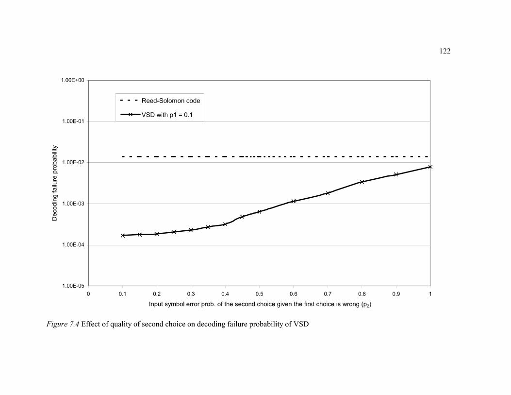
122

Figure 7.4 Effect of quality of second choice on decoding failure probability of VSD

1.00E-05

1.00E-04

1.00E-03

1.00E-02

1.00E-01

1.00E+00

0 0.1 0.2 0.3 0.4 0.5 0.6 0.7 0.8 0.9 1

Input symbol error prob. of the second choice given the first choice is wrong (p2)

Dec

odin

g fa

ilure

pro

babi

lity

Reed-Solomon code

VSD with p1 = 0.1

123

Figure 7.5 Effect of quality of second choice on post-decoded symbol error probability of VSD

1.00E-06

1.00E-05

1.00E-04

1.00E-03

1.00E-02

1.00E-01

1.00E+00

0 0.1 0.2 0.3 0.4 0.5 0.6 0.7 0.8 0.9 1Input symbol error prob. of the second choice given the first choice is wrong (p2)

Post

-dec

oded

sym

bol e

rror p

roba

bilit

y Reed-Solomon codeVSD with p1 = 0.1

124

Figure 7.6 Decoding failure probability of VSD and Non-interleaved Reed-Solomon code with errors only and a mixture of errors

and erasures (32-bit symbols, random inner code,2-state fading channel)

1.00E-06

1.00E-05

1.00E-04

1.00E-03

1.00E-02

1.00E-01

1.00E+00

0.445 0.45 0.455 0.46 0.465 0.47 0.475 0.48 0.485 0.49 0.495

Probability of bit erasure for the two-state fading channel (Pera)

Dec

odin

g fa

ilure

pro

babi

lity

Reed-Solomon code(errors only)Reed-Solomon code(errors & erasures)VSD

125

Figure 7.7 Post-decoded symbol error probability of VSD and Non-interleaved Reed-Solomon code (32-bit symbols, random

inner code, 2-state fading channel)

1.00E-07

1.00E-06

1.00E-05

1.00E-04

1.00E-03

1.00E-02

1.00E-01

1.00E+00

0.445 0.45 0.455 0.46 0.465 0.47 0.475 0.48 0.485 0.49 0.495

Probability of bit erasure for the two-state fading channel (Pera)

Post

-dec

oded

sym

bol e

rror p

roba

bilit

y

Reed-Solomon code(errors only)

VSD

126

Figure 7.8 Decoding failure probability of VSD and Non-interleaved Reed-Solomon code (15-bit symbols, frequency-hopping, 60

users, 9 chips/row, efficiency = 0.389)

1.00E-06

1.00E-05

1.00E-04

1.00E-03

1.00E-02

1.00E-01

1.00E+00

0.02 0.04 0.06 0.08 0.1 0.12 0.14Input symbol error probability of the first choice (p1)

Dec

odin

g fa

ilure

pro

babi

lity

Reed-Solomon codeVSD

127

Figure 7.9 Post-decoded sytmbol error probability of VSD and Non-interleaved Reed-Solomon code (15-bit symbols, frequency-

hopping, 60 users, 9 chips/row, efficiency = 0.389)

1.00E-06

1.00E-05

1.00E-04

1.00E-03

1.00E-02

1.00E-01

1.00E+00

0.02 0.04 0.06 0.08 0.1 0.12 0.14

Input symbol error probability of the first choice (p1)

Post

-dec

oded

sym

bol e

rror p

roba

bilit

y

Reed-Solomon codeVSD

128

Figure 7.10 Effect of vector symbol size on the decoding failure probability of VSD

1.00E-06

1.00E-05

1.00E-04

1.00E-03

1.00E-02

0.04 0.05 0.06 0.07 0.08 0.09 0.1 0.11 0.12 0.13 0.14

Input symbol error probability of the first choice (p1)

Dec

odin

g fa

ilure

pro

babi

lity

32-bit symbol

24-bit symbol

16-bit symbol

16-bit symbol withextra step

Chapter 8

INTERLEAVED REED-SOLOMON CODES

To minimize the likelihood of dependent errors for VSD, the vector symbols

should consist of at least 24 or 32 bits as seen in section 7.2.3. The symbol size restriction

of VSD leads to difficulty in comparing the performance of VSD with Reed-Solomon

codes. With the assumption of 32-bit symbols, the performance of VSD is shown to be

much better than Reed-Solomon code of the same number of bits. However Reed-

Solomon codes usually use fewer bits such as 8 bits per symbol. To handle a larger size

symbol, the common practice is to interleave many Reed-Solomon codes. Kasami

showed an example of interleaving 9 Reed-Solomon codes to achieve 72-bit symbols in

[23] and 5 Reed-Solomon codes to achieve 40 bit symbols in [24]. Jensen and Passke also

used interleaved Reed-Solomon code with inner sequential decoding in [25]. For a large

symbol size, VSD becomes more and more attractive since it can handle 32 or more

bits/symbol easily. Interleaving does improve the performance of Reed-Solomon code for

large symbol size. Therefore, to make the comparison between VSD and Reed-Solomon

codes fairer, interleaved Reed-Solomon codes are considered in this chapter.

In the comparison, when the inner code provides 24-bit symbols, VSD will use

24-bit symbols directly. However Reed-Solomon code will break the 24-bit symbols into

smaller size such as three 8-bit subblocks/symbol. Then three Reed-Solomon codes are

combined, each of which handles 8-bit subblocks (or 8-bit symbols since each of the

three codes will consider each 8-bit subblock as a symbol). As a result, the relationship

130

between the symbol probabilities of the large vector symbol (e.g., 24-bit) and the small

subblocks (e.g., 8-bit) is of interest. Unfortunately, there is no general rule for this

relationship. Given a different code, the relationship between different symbol sizes in

terms of symbol error probability can be totally different.

In general, powerful inner codes have high minimum distance and are designed to

correct a large number of errors. When their decoders make a wrong decision, which

means that they decide that the received block corresponds to a wrong codeword, they

tend to leave many data errors in all or most parts of the decoded block. This is because

each code word has a minimum distance that they differ from each other. For a block

code with minimum distance dmin, a wrong decision will lead to at least dmin error bits in

the code word. Since the code word consists of both data and check bits, some of the

error bits may be check bits and will be disregarded at the outer code decoder. Therefore,

the number of data bits in error and the positions of the errors still depend on the structure

of the code. However, the idea of dmin suggests that the symbol selected from double the

number of bits should have less than double the symbol error probability. The results in

this chapter show that this is true for the three different inner codes in consideration.

One effect of interleaving many Reed-Solomon codes, where each of them handle

subblocks, is that all codes must be successful in order for the received sequence to be

successfully decoded. This means that the effective block error probability for the total

interleaved Reed-Solomon code is higher than for an 8-bit-symbol individual code part

by some factor that is more than 1. This factor depends on the correlation of errors among

131

subblocks, which in turn depends both on the structure of inner codes and the degree of

burstiness of the channel.

8.1 Examples of Relationship between the Symbol Error Probabilities of the Vector

Symbols and their Subblocks

The relationship between the symbol error probabilities of the vector symbols and

their subblocks depends highly on the structure of the inner code. Therefore, we do not

attempt to generalize the results, but to give some examples of what they are.

In Table 8.1-8.3, the inner code is a (2,1,4) convolutional inner code with G(D) =

[1+D+D4 1+D+D3+D4] and dfree = 5. The channels are simplified two-state fading

channel, AWGN channel and Rayleigh fading with AWGN channel. It is seen from these

tables that the ratio of symbol error probability of 24-bit symbols and that of 8-bit

symbols (or subblocks) is much lower than the ratio of the number of bits between the

two symbol sizes. Specifically, the ratio of the number of bits is 24/8 = 3 and if only one

subblock is always wrong when the whole 24-bit symbol is wrong, the ratio of the

symbol error probability should be 3 too. However, the ratio of the symbol error

probability is about 1.8 – 2, which is much lower than 3 at least in the range of interest.

This means that when the 24-bit symbol is wrong, more than one subblock are often

wrong too. The results from these three tables will be used in the simulations in Section

8.2.

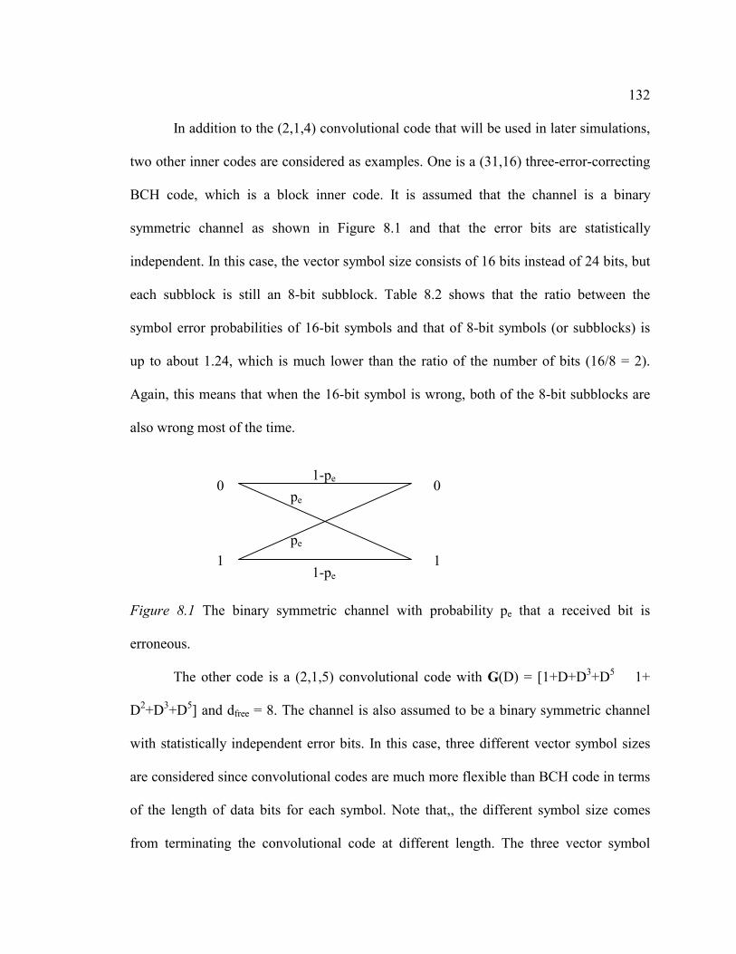
132

In addition to the (2,1,4) convolutional code that will be used in later simulations,

two other inner codes are considered as examples. One is a (31,16) three-error-correcting

BCH code, which is a block inner code. It is assumed that the channel is a binary

symmetric channel as shown in Figure 8.1 and that the error bits are statistically

independent. In this case, the vector symbol size consists of 16 bits instead of 24 bits, but

each subblock is still an 8-bit subblock. Table 8.2 shows that the ratio between the

symbol error probabilities of 16-bit symbols and that of 8-bit symbols (or subblocks) is

up to about 1.24, which is much lower than the ratio of the number of bits (16/8 = 2).

Again, this means that when the 16-bit symbol is wrong, both of the 8-bit subblocks are

also wrong most of the time.

0 0

1 1

Figure 8.1 The binary symmetric channel with probability pe that a received bit is

erroneous.

The other code is a (2,1,5) convolutional code with G(D) = [1+D+D3+D5 1+

D2+D3+D5] and dfree = 8. The channel is also assumed to be a binary symmetric channel

with statistically independent error bits. In this case, three different vector symbol sizes

are considered since convolutional codes are much more flexible than BCH code in terms

of the length of data bits for each symbol. Note that,, the different symbol size comes

from terminating the convolutional code at different length. The three vector symbol

pe

pe

1-pe

1-pe

133

sizes are 16, 24 and 32 bits. Each of them is broken up into two, three and four 8-bit

subblocks/symbol, respectively. Table 8.3 shows the results for the three symbol sizes.

Similar to the results of the two previous codes, the ratio between the symbol error

probability of the large vector symbols (16, 24 or 32 bits) and that of the 8-bit subblocks

are much smaller than the ratio of the number of bits (2,3 and 4 respectively).

Table 8.1 Comparison of symbol error probability for 8-bit subblock and 24-bit symbol

using a (2,1,4) convolutional code with dfree = 5

a) in two-state fading channel.

Pera

Symbol error

probability (8 bit)

Symbol error

probability (24 bit) Ratio of 24 bit/ 8bit

0.380 0.0292 0.0589 2.0136

0.385 0.0325 0.0650 1.9975

0.390 0.0361 0.0716 1.9823

0.395 0.0399 0.0786 1.9821

0.400 0.0440 0.0859 1.9674

0.405 0.0485 0.0940 1.9364

0.410 0.0533 0.1025 1.9223

0.415 0.0588 0.1121 1.9061

0.420 0.0645 0.1220 1.8902

134

Table 8.1 b) in AWGN channel.

Eb/No (dB)

Symbol error

probability (8 bit)

Symbol error

probability (24 bit) Ratio of 24 bit/ 8bit

1.8 0.0624 0.1153 1.8491

1.9 0.0556 0.1038 1.8669

2.0 0.0493 0.0930 1.8853

2.1 0.0436 0.0829 1.9026

2.2 0.0384 0.0736 1.9201

2.3 0.0336 0.0652 1.9378

2.4 0.0294 0.0576 1.9584

2.5 0.0256 0.0506 1.9771

2.6 0.0222 0.0442 1.9943

2.7 0.0191 0.0385 2.0159

Table 8.1 c) in Rayleigh fading with AWGN channel.

Average received

power in dB

(10logR2*Eb)

Symbol error

probability (8 bit)

Symbol error

probability (24 bit) Ratio of 24 bit/ 8bit

6.0746 0.1238 0.2140 1.7280

6.5442 0.0807 0.1450 1.7968

6.7251 0.0676 0.1233 1.8245

6.9897 0.0516 0.0962 1.8645

7.2464 0.0392 0.0746 1.9039

7.4135 0.0325 0.0627 1.9281

7.5774 0.0269 0.0526 1.9548

7.8176 0.0203 0.0404 1.9854

135

Table 8.2 Comparison of symbol error probability for 8-bit subblock and 16-bit symbol

using the (31,16) three-error-correcting BCH code in binary symmetric channel.

Bit error

probability

Symbol error

probability (8 bit)

Symbol error

probability (16 bit)

Ratio of 16 bit/

8bit

0.050 0.0721 0.0814 1.1290

0.060 0.0750 0.0930 1.2400

0.070 0.1315 0.1630 1.2395

0.080 0.1770 0.2100 1.1864

0.090 0.2543 0.2929 1.1518

0.100 0.3130 0.3620 1.1565

0.125 0.4710 0.5540 1.1762

0.150 0.6080 0.7040 1.1579

0.175 0.7360 0.8140 1.1060

0.200 0.8220 0.9240 1.1241

136

Table 8.3 Comparison of symbol error probability using a (2,1,5) convolutional code with

dfree = 8 in binary symmetric channel.

a) 8-bit subblock and 16-bit symbol

Bit error

probability

Symbol error

probability (8 bit)

Symbol error

probability (16 bit) Ratio of 16 bit/ 8bit

0.050 0.0042 0.0054 1.2689

0.060 0.0073 0.0093 1.2740

0.070 0.0120 0.0170 1.4167

0.080 0.0225 0.0320 1.4222

0.090 0.0470 0.0600 1.2766

0.100 0.0585 0.0750 1.2821

0.125 0.1240 0.1600 1.2903

0.150 0.2030 0.2540 1.2512

0.175 0.3270 0.4020 1.2294

0.200 0.4770 0.5780 1.2117

0.225 0.5800 0.6840 1.1793

137

Table 8.3 b) 8-bit subblock and 24-bit symbol

Bit error

probability

Symbol error

probability (8 bit)

Symbol error

probability (24 bit) Ratio of 24 bit/ 8bit

0.060 0.0110 0.0197 1.791

0.065 0.0162 0.0263 1.623

0.070 0.0217 0.0360 1.659

0.075 0.0267 0.0448 1.678

0.080 0.0436 0.0720 1.651

0.085 0.0439 0.0732 1.667

0.090 0.0578 0.0995 1.721

0.095 0.0716 0.1180 1.648

0.100 0.0845 0.1340 1.586

0.150 0.3280 0.4800 1.463

0.200 0.5964 0.7873 1.320

138

Table 8.3 c) 8-bit subblock and 32-bit symbol

Bit error

probability

Symbol error

probability (8 bit)

Symbol error

probability (32 bit) Ratio of 32 bit/ 8bit

0.060 0.0125 0.0280 2.240

0.065 0.0184 0.0400 2.174

0.070 0.0249 0.0540 2.169

0.075 0.0350 0.0732 2.091

0.080 0.0460 0.0970 2.109

0.085 0.0602 0.1195 1.985

0.090 0.0720 0.1400 1.944

0.095 0.0904 0.1730 1.914

0.100 0.1145 0.2100 1.834

0.150 0.3910 0.6020 1.540

0.200 0.6700 0.9040 1.349

139

8.2 Results of VSD in Comparison with the Interleaved Reed-Solomon Code

The simulations will be done for a convolutional inner code in three different

channels. They are not done for the randomly chosen inner code because the relationship

between vector symbols and their subblocks depends highly on the structure of the inner

code. Since the structure of the inner code is unknown for randomly chosen inner codes,

the decoding failure probability of interleaved Reed-Solomon code cannot be computed

accurately.

8.2.1 A Convolutional Inner Code in a Simplified Two-State Fading Channel

In this case, the channel is the simplified two-state fading channel where the

received bit is either error-free or erased. The maximum distance code is constructed

from interleaving many Reed-Solomon codes instead of using only one Reed-Solomon

code with a large vector symbol size directly as done in Chapter 7. VSD uses a

terminated (3,2,2) convolutional outer code with G(D) from Equation (3.37) and H

matrix from Equation (3.38). The lists of two alternative choices are assumed and these

lists result from LVA. In addition, there are 21 vector symbols for each received block

and the symbols are 24-bit symbols. The inner code is a terminated (2,1,4) convolutional

code with G(D) = [1+D+D4 1+D+D3+D4] and dfree = 5. Each inner code sequence is

terminated at 24 data bits to provide a 24-bit vector symbol to the outer code. For the

maximum distance code, three (21,10) Reed-Solomon codes with 8-bit symbols are

interleaved to achieve the 24-bit symbol requirement for the comparison. Since the

140

decoding of the overall maximum distance code fails when at least one of the interleaved

codes fails, the decoding failure is discovered from the simulations too. Figure 8.2 shows

that the decoding failure probability of VSD is still almost an order of magnitude lower

than that of the maximum distance code, which has the same total number of bits. Since

VSD uses 24-bit symbols, while each of the three Reed-Solomon codes uses 8-bit

symbols, the post-decoded symbol error probability is misleading and not shown.

8.2.2 A Convolutional Inner Code in an AWGN Channel

The vector symbols are from the same (2,1,4) terminated convolutional inner code

with 24 data bits per block. The channel is an additive white Gaussian noise (AWGN)

channel, instead of the simplified two-state independent fading channel. Consequently,

the inner decoder is LVA with list of two, where its metric for soft decision decoding is

as described in Section 4.1.2. For the outer code, VSD with the same (3,2,2)

convolutional code and 21 outer symbols is compared with the interleaved Reed-

Solomon code, which consists of three 8-bit-symbol (21,10) Reed-Solomon codes. Figure

8.3 shows that given the same received Eb/No, the decoding failure probability of VSD is

about half an order of magnitude lower than that of Reed-Solomon code in this case.

141

8.2.3 A Convolutional Inner Code in a Rayleigh Fading with AWGN Channel

The assumptions in this case are exactly the same as in the previous case except

that the channel is a Rayleigh fading with AWGN channel instead of simply an AWGN

channel. The fading is assumed to be independent for each bit and follows the Rayleigh

distribution, which can result from interleaving a long sequence of bits. The metric for

this present channel is described in Section 4.1.3. The inner code and the outer codes are

the same as in the previous section. Figure 8.4 shows that given the same average

received power, the decoding failure probability of Reed-Solomon code is more than

twice that of VSD at average received power of 7.81 dB and it is more than six times that

of the VSD at the average received power of 6.73 dB. Note that,, the average received

power is 10log(R2*Eb) where R is the Rayleigh parameter and Eb is the energy per bit.

142

Figure 8.2 Decoding failure probability of VSD (24-bit symbols) and Interleaved Reed-Solomon code (8-bit subblocks), 2-state

fading channel.

1.00E-06

1.00E-05

1.00E-04

1.00E-03

1.00E-02

1.00E-01

0.375 0.38 0.385 0.39 0.395 0.4 0.405 0.41 0.415 0.42 0.425

Probability of bit erasure for the two-state fading channel (Pera)

Dec

odin

g fa

ilure

pro

babi

lity

Reed-Solomon codeVSD

143

Figure 8.3 Decoding failure probability of VSD (24-bit symbols) and Interleaved Reed-Solomon code (8-bit subblocks), AWGN

channel.

1.00E-06

1.00E-05

1.00E-04

1.00E-03

1.00E-02

1.00E-01

1.5 1.7 1.9 2.1 2.3 2.5 2.7 2.9

Eb/No (dB)

Dec

odin

g fa

ilure

pro

babi

lity.

Reed-Solomon codeVSD

144

Figure 8.4 Decoding failure probability of VSD (24-bit symbols) and Interleaved Reed-Solomon code (8-bit subblocks), Rayleigh

fading with AWGN channel

1.00E-07

1.00E-06

1.00E-05

1.00E-04

1.00E-03

1.00E-02

1.00E-01

1.00E+00

5.5 6 6.5 7 7.5 8

Average received power in dB

Dec

odin

g fa

ilure

pro

babi

lity

Reed-Solomon codeVSD

Chapter 9

METHOD & RESULTS ON PERFORMANCE OF VSD FOR FIRST

INFORMATION BLOCK (FIB)

In addition to the large vector upper bound on the decoding failure probability in

chapter 6, the weight distribution can be used to gain some insight on the number of

syndromes needed for each successful decoding of the first information block. This gives

a very rough estimate of the complexity of the decoder. As described in Section 3.2, FIB

is a block of received symbol sequence that starts with the first yet undecoded received

symbol. The more syndromes the decoder is using, the longer the block of FIB.

To consider FIB instead of a terminated convolutional code in the case of the

large vector union upper bound, the received sequence is assumed to be infinite. In other

words, more received symbols are always available if they are needed for the decoding.

However, the maximum number of syndromes used is limited to sixteen for the

simulations. Even though the idea of the weight structure is similar to the one used on

section 6.1 to find the large vector union upper bound, the different assumptions make it

necessary to redefine some of the parameters. For clarity, the definitions for this section

is presented as follows:

146

Assumption: The error symbols are linearly independent. Each symbol is independent

identically distributed with probability of error p1 and p2 for the first and second choice

symbols respectively.

Define:

p1 = symbol error probability of the first choice. (q1 = 1- p1)

p2 = symbol error probability of the second choice given that the first choice is wrong.(q2

= 1-p2)

t = index of the interval on the trellis diagram which equals to the number of

syndromes used for decoding at that interval.

Note: The interval t starts at the first departure from zero of the trellis diagram.

Ft = probability of failure at the end of t intervals due to error symbol completely

covering or one position away from covering (without any correct second choice)

a binary code word that starts with non zero path in the trellis diagram (i.e., the

first two positions of the symbol sequence that we are trying to correct are non

zero.)

Ft np

= the same as Ft except we assume that the decoder does not recognize any pair of

error symbols that have incorrect first choices and correct second choices. (This

idea will be discussed more when Ft np is computed.)

tNs(w) = number of code word paths of weight w at state s and at the end of interval t.

tN’(w) = Σs[tNs(w)] = Total number of code word path of weight w at the end of interval

t. Note that,, this tN’(w) is different from tN(w) since the code is not terminated.

147

tPsynd = Probability of failure to decode the first information block using a maximum of

t syndromes.

To demonstrate this recursive method, a (2,1,2) convolutional code with G(D) =

[1+D2,1+D+D2] will be used as an example. The method can be extended to other

convolutional codes with some modifications. However, it is not important to extend this.

The purpose of this method is to gain some insight in the number of syndromes needed

for each successful decoding of a FIB. To find the performance of VSD in terms of the

decoding failure probability, the large vector upper bound or the computer simulation are

more appropriate. There are mainly 3 steps for this method as follows:

9.1 Compute tNs(w) and tN’(w) (the Weight Structure):

The tNs(w) equations were discovered in section 6.1. For convenience, the equations

are repeated here.

For this (2,1,2) code, the recursive functions for finding tNs(w) are, (for t > 1):

tN0(w) = t-1N1(w-2) + t-1N0(w); t > 1 (9.1)

tN1(w) = t-1N2(w-1) + t-1N3(w-1); t > 1 (9.2)

tN2(w) = t-1N1(w); t > 1 (9.3)

tN3(w) = t-1N3(w-1) + t-1N2(w-1); t > 1 (9.4)

For t = 1, there is only one binary codeword of weight two.

148

Note that,, the term t-1N0(w-2) is omitted from equation (9.3) because once the path goes

back to state 0, all continuing paths are included in the computation of Ft and Ft np

.

Then, tN’(w) is computed from Σs[tNs(w)].

9.2 Find Union Upper Bound on Ft and Ft np

:

Using equation (9.5) and (9.6) as follows:

Ft ≤ (p1p2)2{Min(1, Σw [tN’(w)*( p1w-2 + (w-2)q1(p1p2)w-3)]}

+ 2q1p1p2{Min(1, Σw[tN’(w)*( p1p2)w-2)]}

+ 2p12q2p2{Min(1, Σw[tN’(w)* p1

w-2)]}; t = 1,2,3… (9.5)

Ft np

≤ Ft + (p1q2)2*{Min(1, Σw[tN’(w)* p1 w-2)]}; t = 1,2,3… (9.6)

The first term in equation (9.5) is for the case that the two received symbols in the

first interval has both choices wrong (p1p2)2. The term p1w-2 means that the rest of the

“1’s” positions also have first choices wrong. The term q1(p1p2)w-3 means that in the rest

of the “1’s” positions, there is one correct first choice, while other “1’s” positions have

all first and second choices wrong. The one correct first choice can be in any of the (w-2)

position, so this term is multiplied by (w-2). The second term in (9.5) is for the case that

one of the two received symbols has correct first choice while the other has both choices

wrong (q1p1p2). There are two ways this can happen, so it is multiplied by two. The term

149

(p1p2)w-2 means that the rest of the “1’s” positions have both first and second choice

wrong. The third term in (9.5) is for the case that one of the two received symbols has

both choices wrong while the other has incorrect first choice and correct second choice

(p12q2p2). There are two ways this can happen, so it is multiplied by two.

The additional term in equation (9.6) is for the case that the two received symbols

have incorrect first choices and correct second choices. This additional term is included

in Ft np, but not in Ft because this term is considered as a failure event except in the first

interval. The distinction should become clear when tPsynd is computed. For the first

interval, we can correct this pair by using only one syndrome. To demonstrate this, let the

error matrix E = [e1’ e2’]T. With one syndrome case, the (binary) H matrix = [1 1] and the

syndrome matrix S = [e1’+ e2’]. Append the differences of the two choices and also the

sum of the differences (done only for the one syndrome case). The new syndrome matrix

is S’ = [(e1’+ e2’) e1’ e2’ (e1’+ e2’)]T. The decoder will recognize the duplication of the

first and the last element and the true errors are readily revealed as e1’ and e2’.

Additional note on equation (9.5) and (9.6):

a) Min (1, a) is included because all the terms that correspond to “a” in equation (9.5)

and (9.6) are probabilities and thus, they cannot exceed 1.

b) Equation (9.5) and (9.6) give exact results for t = 1 case.

c) To speed up the computation, the limit of the summations goes from w = 3 to w = 2t.

(The minimum weight is 3 when t >1 for this code and in general, the weight cannot

go beyond the number of outputs times the number of intervals.)

150

9.3 Find tPsynd (Probability of Failure to Decode FIB Using a Maximum of t

Syndromes):

We use union bound to find this probability. The decoder that can use a maximum

of t syndromes will fail if

1) The code words that depart the trellis at t = 0 (i.e., the beginning of the first interval)

are covered or one position away from being covered by error symbols without any

correct second choice. The corresponding probability is Ft.

2) The code words that depart the trellis at the end of interval t = 1,2,3,… are completely

covered or one position away from covered by error symbols without any correct

second choice. Since they depart at a later interval, the associated probability is Ft-i np

where i indicates the interval that the code words depart. In addition, a particular Ft-i np

is taken into account only when the decoder fails with i syndromes.

Therefore, tPsynd can be found by:

tPsynd ≤ Ft + 1Psynd *(Ft-1 np) + 2Psynd *(Ft-2

np) + … + t-1Psynd *(F1 np) (9.7)

9.4 Expected Number of Syndromes Used in Decoding FIB:

This can be calculated as follows:

E{# of syndromes used}

= { ∑−

=

⋅1maxt

1tt P(success with exactly t syndromes) }+ tmax P(success with at least tmax

syndromes)

151

= { ∑−

=

⋅1maxt

1tt [P(success with maximum of t syndromes) - P(success with maximum of t-1

syndromes)]} + tmax P(failure with maximum tmax –1 syndromes)

= { ∑−

=

⋅1maxt

1tt [(1 - tPsynd) – (1 - t-1Psynd)]} + tmax (tmax-1Psynd)

= { ∑−

=

⋅1maxt

1tt [ t-1Psynd - tPsynd] } + tmax (tmax-1Psynd) (9.8)

where tmax = maximum number of syndromes that the decoder will use.

9.5 Complexity of VSD with Maximum of tmax Syndromes:

To be very conservative, we assume that this complexity (relative to the one

syndrome case) is the cube of the number of syndromes used. The cubic rise is assumed

because the error values can generally be evaluated by inverting a matrix with dimension

less than the number of syndromes used. However, this is pessimistic because we can

often do simple forward substitution to find error values and the matrix inversion is not

needed [17] In addition, the matrix is binary, and each XOR operation can be used on a

word, which consists of many bits such as 32-bit word, instead of on each bit. This idea

was described in section 7.1.3. Therefore, even if the matrix inversion is necessary, the

cubic rise is still pessimistic. Based on the cubic rise assumption and Equation (9.8), we

obtain

152

Complexity (relative to one syndrome case)

≤ { ∑−

=

1maxt

1t

3t [ t-1Psynd - tPsynd] } + tmax3 (tmax-1Psynd) (9.9)

9.6 Complexity Comparison between VSD and RS Decoder

The complexity of VSD is comparable to that of an RS decoder. To show this, the

complexity in terms of the number of computations per decoded bit (suggested by

Metzner) is considered for both decoders. For an RS decoder, we assume the fast

generalized-minimum distance decoding proposed by Sorger [61]. This decoder uses a

modified Berlekamp-Massey algorithm [12,62]. The optimal asymptotic generalized-

minimum distance decoding complexity is O (d*N), where N is the number of outer

symbols and d is the distance of the code [61]. This complexity is counted as the number

of multiplications in the field [63]. For each field multiplication, suppose the dual basis

multiplication algorithm by Berlekamp [64] is used. The complexity of this multiplier is

O(r), where the Reed-Solomon code is over GF(2r), since the realization circuit requires

O(r) gates [13]. Notice that whether the Reed-Solomon code is interleaved or not, the

complexity is still of the same order with this multiplication technique. There are r*K

decoded bits per each received sequence for an (N,K) Reed-Solomon code. Therefore, the

complexity of the RS decoder in terms of the number of computations per decoded bit is

roughly O((d*N*r)/(r*K)), which is O(d*N/K) for the RS decoder.

For VSD, assume that the (2,1,2) convolutional code is used and it is terminated

to have N outer symbols and K data symbols. Note that,, a Reed-Solomon code can be

153

shortened or punctured so that it has the same data length and data rate as this terminated

convolutional code. Suppose N is 32, and then K will be 14. Assume that the

convolutional VSD uses x = 16 syndromes immediately without trying fewer number of

syndromes first. This makes the convolutional VSD similar to block VSD. It also

increases the complexity of convolutional VSD, but it will make the comparison simpler.

Since H is a binary matrix, a row or a column of H can be represented by one or a few

words. In the C++ programming used in this thesis, a word contains 32 bits. Then bitwise

XOR can be used to perform a column or a row operation. The following estimate of the

complexity is a rough estimate. Only the main steps that need most computations are

considered. These steps are the one that requires Gauss-Jordan operation. Suppose N =

32, K = 14 and number of syndromes = 16. Note that,, these numbers are used to make

the explanation clearer. Even if these parameters are changed, the order of the complexity

will be the same. We use the notations from Section 3.1 and 3.2.

1) Gauss-Jordan operation is performed to

a) Discover whether any appended row is in the row space of S. The Gauss-Jordan

operation is performed on the modified syndrome matrix S’. Since there are 16

syndromes and it is a rate ½ convolutional code with lists of two, there are 48

rows in S’ (including the appended rows). Each column can then be presented by

two 32-bit words and at most 2r computations for each row are needed for at most

x rows, where x is the number of syndromes (x = 16). The factor of 2 comes from

the fact that each operation needs to works on two words. For larger lists or larger

number of syndromes (x > 21 with lists of two), the factor will be higher

154

depending on the number of words needed to represented one column. The

operations are basically interchanging two columns or performing bitwise XOR

between two columns. Thus, there are at most 2*r*x computations for r*K

decoded bits for the Gauss-Jordan in this step. The number of computations per

decoded bit is approximately 2*x/K for this step. For rate ½ code, this is

2*(N/2)/K = N/K. For other rate, the number of computations per decoded bit will

be some factor times N/K.

b) The error-locating vector is the “OR” of the linearly independent null

combinations. The null combinations are discovered by performing Gauss-Jordan

reduction on S”, which contains x rows. With x = 16, each column can be

represented by a word. This step adds an additional x/K computations/decoded

bit.

c) Invert Hsub matrix to find error values. With e error symbols, this binary matrix

has a dimension of e by e. This adds another e/K computations per decoded bit.

2) Suppose that data scrambling is necessary. Assume that the transformations for

different vector symbols in data scrambling technique are multiplications of different

field elements. Then, there are N field multiplications. Each of them can be realized by

dual basis multiplication algorithm with the complexity of O(r). The number of decoded

bits are still r*K. Thus, the number of computations per decoded bit for this step is in the

order of (N*r)/(r*K) = N/K.

Therefore, the estimate number of computations per decoded bit for VSD is the

order of 2*x/K + x/K + e/K + N/K, which means that the complexity is O(N/K) since the

155

number of syndromes x is N/2 for rate ½ code and e is much less than N. This complexity

is in terms of the number of computations per decoded bit. Recall that the number of

computations per decoded bit for RS decoder is O(d*N/K). As a result, VSD has roughly

comparable complexity as the RS decoder.

9.7 Results of Decoding Failure Probability for FIB

The results are for the (2,1,2) convolutional outer code with 32-bit symbols from

(72,32) randomly chosen block inner code in simplified two-state fading channel. The

error statistics (p1 and p2) for this inner code was shown in Table 5.4. Figure 9.1

illustrated the upper bound on probability of failure to decode the first information block

(FIB) with different number of maximum syndromes allowed. Note that,, the decoder

does not use this maximum number of syndrome for every decoding attempt. In fact, it

rarely uses more than one syndrome. This maximum number of syndromes is the limit

that the decoder will not attempt to decode with more syndromes if it has failed with

maximum number of syndromes allowed. The exact performances are illustrated for the

one and two syndromes. The upper bound performances are shown for the two, four,

eight and sixteen syndromes. It is obvious that this decoding technique is very powerful

even for a very simple convolutional code. For example, with p1 = 0.047 and p2 = 0.263,

this probability of failure is upper bound around 7*10-7 with maximum of 8 syndromes. It

is as expected that higher number of maximum syndromes allowed provides better

decoding performance for VSD. Significant gains are achieved by increasing the

156

maximum number of syndromes from one to two, two to four and four to eight. However,

the gain is considerably less when the maximum number of syndromes is increased from

eight to sixteen. This gain does increase for the higher value of p1 as expected. This is

because for lower range of p1, most of the correctable error events that occur can be

corrected with at most 8 syndromes. For higher range of p1, there are more error symbols

and therefore more error events that need more number of syndromes to correct.

Figure 9.2 shows that the expected number of syndromes used by the decoder for

different symbol error probabilities are very low even up to symbol error probability of

0.139, which is a very high symbol error probability of the first choice. This shows that

most of the time, only one syndrome is needed. Figure 9.3 shows the expected (relative)

complexity as a function of symbol error probability, which is also very low up to symbol

error probability of about 0.139. For example, even with symbol error probability of

0.139, the decoder needs only one syndrome for 87.1% of the time and two syndromes

for 10.9% of the time and more than two syndrome for about 2% of the time. Note that,,

the maximum number of syndromes used for both Figure 9.2 and 9.3 is sixteen. While

Figures 9.1-9.3 use the error statistics (p1 and p2) from the randomly chosen inner code,

Figure 9.4 shows the effect of the quality of the second choice by fixing the symbol error

probability of the first choice. It is as expected that lower p2 (i.e., better quality of the

second choice) results in better decoding performance of VSD. Note that,, the decoder

should use the more likely received symbol as the first choices since it achieves better

performance when p1 = 0.1 and p2 = 0.2 than when p1 = 0.2 and p2 = 0.1.

157

Figure 9.1 Performance of VSD for a (2,1,2) convolutional outer code. (exact values for 1 and 2 syndromes, upper bound for

2,4,8 and 16 syndromes)

1.00E-07

1.00E-06

1.00E-05

1.00E-04

1.00E-03

1.00E-02

1.00E-01

1.00E+00

0.020 0.040 0.060 0.080 0.100 0.120 0.140 0.160

Input symbol error probability of the first choice (p1)

Upp

erbo

und

on p

roba

bilit

y of

failu

re w

ith m

ax t

synd

rom

es

2 syndromesexact

1 syndromeexact

4 syndromes,bound

2 syndromes,bound

8 syndromes,bound

16 syndromes,bound

158

Figure 9.2 Average number of syndromes used in VSD for a (2,1,2) convolutional outer code.

0

0.5

1

1.5

2

2.5

0.020 0.040 0.060 0.080 0.100 0.120 0.140 0.160

Input symbol error probability of the first choice (p1)

Exp

ecte

d nu

mbe

r of s

yndr

omes

use

d

159

Figure 9.3 Expected complexity of VSD (relative to the one syndrome case) for a (2,1,2) convolutional outer code

0

1

2

3

4

5

6

0.020 0.040 0.060 0.080 0.100 0.120 0.140 0.160

Input Symbol error probability of the first choice (p1)

Rel

ativ

e co

mpl

exity

(com

pare

with

the

one

sym

drom

e ca

se)

160

Figure 9.4 Effect of the quality of the second choice on the performance of VSD

1.00E-05

1.00E-04

1.00E-03

1.00E-02

1.00E-01

1.00E+00

0 0.05 0.1 0.15 0.2 0.25 0.3

Symbol error prob. of the second choice given that the first choice is wrong (p2)

Upp

erbo

und

on p

roba

bilit

y of

failu

re w

ith m

ax k

syn

drom

es

2 syndromes, exact, p1 = 0.1

4 syndromes, bound, p1 =0.1

2 syndromes, exact, p1 = 0.2

4 syndromes, bound, p1 =0.2

2 syndromes, exact, p1 = 0.1, no second choice

4 syndromes, bound, p1 = 0.1, no second choice

Chapter 10

DISCUSSIONS & CONCLUSIONS

Vector symbol decoding (VSD) with lists of alternative vector symbol choices for

outer convolutional codes has been presented. Convolutional VSD is different from block

VSD and maximum distance code decoding in that it often requires only one or a few

syndromes in each decoding attempt of FIB. After each successful decoding,

convolutional VSD can move ahead and consider the next FIB and so on. However, block

VSD and maximum distance code decoding can only decode when it has received the

whole block. This means that convolutional VSD generally requires fewer computations

since the number of computations increases more than linearly with the number of

syndromes involved.

The use of lists of alternative vector symbol choices is shown to improve the

performance of VSD. It is seen that even with very short lists (i.e., lists of two)

considered in this thesis, the effect is significant. The degree of improvement depends on

the quality of the alternative choices. Since the thesis focus on the lists of two choices,

the effect of the quality of the second choice is illustrated. If longer lists are considered,

the performance of VSD will be improved especially when the symbol size is large

enough. The lists of two were chosen in this thesis for simplicity. The principle of VSD

with lists allows lists of more than two and variable list size. However, longer lists may

require a more complex inner decoder such as serial LVA with L > 2. In other cases such

162

as a fast frequency-hopping spread spectrum system, lists of three can be obtained with

no additional complexity; only more storage is needed.

The lists can result from many sources such as inner decoders and space diversity.

Some examples of vector symbol sources and channel conditions are considered in this

thesis. Specifically, the vector symbols are from a convolutional inner code, a randomly

chosen inner code, or a fast frequency-hopping spread spectrum system. The channels are

a simplified two-state fading channel, AWGN channel, Rayleigh fading with AWGN

channel and channel with interference. The two-state fading channel is basically a pure

bit erasure channel, where the received bit is either an erasure or an error-free bit.

Rayleigh fading with AWGN channel is assumed to be independent fading according to

the Rayleigh distribution in the bit level with the additive white Gaussian noise. Channel

with interference is assumed to have interferences from other users in the spread

spectrum system, but no additive noise since decoding error is mainly due to

interferences in this type of system.

To obtain the lists of alternative symbol choices, the List Viterbi Algorithm

(LVA) can be used for the convolutional inner code. For the frequency-hopping system,

the decoder is adapted so that it records the second choice as well as the first choice. For

randomly chosen inner codes, there is no practical method to find the alternative choices

by the inner decoder. However, it can provide the average error statistics (p1 and p2) and

it serves as example to illustrate the average quality of the second choice for an (n, k)

randomly chosen code.

163

To simplify the computer simulation of the VSD, only the error statistics (p1 and

p2) and not the actual bit patterns of the vector symbols from various inner codes are

considered. This simplification is required in the case of randomly chosen inner code

because the actual patterns of the vector symbols are not available from the analytical

result. For lists of two choices considered in this thesis, the error statistics are the symbol

error probability of the first choice (p1) and the symbol error probability of the second

choice given that the first choice is wrong (p2). These error statistics are found by

computer simulations for the inner convolutional code and for the frequency hopping

spread spectrum system in different channel conditions. They are found by analytical

method for the randomly chosen code. In the computer simulation of VSD algorithm, it is

assumed, without loss of generality, that an all-zero outer code word is transmitted. The

error symbols are generated according to the error statistics and it is also assumed that on

average, there are the same number of “1’s” and “0’s” in each error symbol.

For the maximum distance code, there are two ways to handle large vector symbol

size. The first one is called “non-interleaved Reed-Solomon code”, where the decoder is

assumed to use the same symbol size as the VSD directly. The second one is called

“interleaved Reed-Solomon code”, where it is constructed from many smaller vector

symbol size Reed-Solomon codes. The interleaved Reed-Solomon code is normally used

when it is needed to handle a large vector symbol size. For example, if the inner decoders

provide 24-bit symbols, VSD will use this symbols directly, while interleaved Reed-

Solomon code will divide each symbol into many smaller blocks such as three 8-bit

subblock/24-bit symbol. Therefore, an 8-bit subblock can be correct even when the 24-bit

164

symbol is wrong. Consequently, the interleaved Reed-Solomon code has a better

performance than the non-interleaved one.

The decoding failure probability of non-interleaved Reed-Solomon code is

computed analytically by using the property of the code that it can correct certain amount

of errors successfully and that it will fail when the number of errors exceeds its correction

capability. Results show that for 32-bit vector symbols from (2,1,4) convolutional inner

code, both the decoding failure probability and the post-decoded symbol error probability

of VSD are about two orders of magnitude lower than that of the non-interleaved Reed-

Solomon code, which has the same number of data bits and encoded bits.

The decoding failure probability of the interleaved Reed-Solomon codes is found

by computer simulations at the inner code level. The simulation is necessary because the

relationship between the symbol error probabilities of different symbol sizes depends

highly on the structure of the inner codes. Some examples of this relationship are shown

for two convolutional codes and for a BCH code in a binary symmetric channel.

Moreover, the correlation between each subblock of the total block of each vector symbol

depends on the inner codes and the burstiness of the channel and cannot be easily

generalized.

15-bit vector symbol from frequency hopping spread spectrum system is also

considered even though VSD is not designed to use this small symbol size. An extra step

is added in order to reduce the decoding failure probability due to the wrong recognitions.

With this extra step, the performance of VSD for the 15-bit symbol is improved, but it is

still worse than the 24-bit and 32-bit symbol case, especially in the low symbol error

165

probability range. Therefore, it is as expected that the decoding failure probability of

VSD will be considerably lower than that of the non-interleaved Reed-Solomon code for

the range that symbol error probability is quite large. The difference is seen to be closer

when the symbol error probability is small and if it is very small, Reed-Solomon code

may eventually have a better performance.

For vector symbols that come from convolutional inner code, they are also

compared with the interleaved Reed-Solomon code. This makes the comparison fairer

since an interleaved Reed-Solomon code provides better performance than the non-

interleaved one and it is usually used to handle large symbol size. The simulations are

done for the (2,1,4) convolutional code in three different types of channels: the simplified

two-state fading channel, AWGN channel and the Rayleigh fading with AWGN channel.

The decoding failure probability of VSD is about an order of magnitude lower than the

interleaved Reed-Solomon code in all three channels. The post-decoded symbol error

probability is not shown since VSD uses 24-bit symbols, while each of the three Reed-

Solomon codes before the interleaving uses 8-bit symbols.

For most comparisons in this thesis, the vector symbols are assumed to be either

error-free or erroneous. The possibility of erasure symbols is usually not considered in

the comparisons because VSD can currently handle errors only although it is possible to

extend VSD to handle both errors and erasures. To make the comparison really fair,

Reed-Solomon codes should be allowed to use both the interleaved Reed-Solomon codes

and have a mixture of errors and erasures. This should then be compared with VSD that

can handle a mixture of errors and erasures; this type of VSD still needs further study. If

166

the VSD with errors only is to be compared with interleaved Reed-Solomon code with a

mixture of errors and erasures, the difference between the performances will be closer.

They will be more competitive. However, it is expected that VSD with a mixture of

errors and erasures will have better performance than VSD with errors only. Therefore, it

is still not clear how close the difference in performance will be between interleaved

Reed-Solomon codes and VSD when both use a mixture of errors and erasures. If the

system is such that there are errors symbols, but no erasure symbols, then the comparison

between VSD with errors only and interleaved Reed-Solomon code with errors only will

be a fair comparison.

The analytical method for computing the performance of randomly chosen outer

codes for VSD with a mixture of errors and erasures are shown in [26]. Comparison

results between a (255,223) maximum distance code and a randomly chosen vector

symbol code are also shown in the same paper and it is seen that for the mixture of errors

and erasures assumption, the performance of VSD is considerably better than that of the

Reed-Solomon code for a long range of symbol error probability and symbol erasure

probability, especially in the severe channel condition. Both VSD and Reed-Solomon

codes use the same 32-bit symbols in the comparisons though. Further investigation is

needed for implementing VSD with a mixture of errors and erasures.

For this thesis, it is assumed that VSD can handle errors only. However, for the

benefit of Reed-Solomon code, Reed-Solomon code is allowed to have a mixture of error

symbols and erasure symbols for the random inner code. Specifically, a comparison of

VSD with errors only and non-interleaved Reed-Solomon code with a mixture of errors

167

and erasures are shown for a randomly chosen inner code in the simplified two-state

fading channel. For this type of inner code and channel, it is relatively easy to compute

the performance of non-interleaved Reed-Solomon code for a mixture of errors and

erasures analytically and the method is shown in Section 7.1.2. The comparison is done

for non-interleaved Reed-Solomon code in this case because the structure of the random

inner code is unknown and thus, the interleaved Reed-Solomon code cannot be used. The

outer code for VSD is the same (3,2,2) convolutional code for VSD with 21 symbols and

the outer code for maximum distance code is the (21,10) Reed-Solomon code. The

comparison result shows that the decoding failure probability of VSD with errors only is

almost half an order of magnitude lower than that of the non-interleaved Reed-Solomon

code with a mixture of errors and erasures for the 32-bit vector symbols from (72,32)

randomly chosen inner code.

One difference between convolutional VSD and the maximum distance code

decoding is that the former handles convolutional outer codes and the later handles block

outer codes. Note that,, the principle of VSD with lists of alternative symbol choices can

decode both block and convolutional outer codes, while maximum distance codes are

only in a restricted class of block codes. Therefore, VSD is more flexible in this aspect

and in particular, convolutional VSD has another advantage in terms of the ease of the

encoder. However, convolutional VSD requires the knowledge of the parity check matrix

of the outer code. This knowledge is well known for systematic convolutional codes, but

not for nonsystematic ones. This is because convolutional codes are usually decoded by

Viterbi decoding algorithm or sequential decoding algorithm [29], both of which do not

168

require this knowledge. Nonsystematic convolutional codes are desirable since they

usually provide better performance than the systematic ones. Therefore, a way to

compute the parity check matrix for any rate 1/2, 2/3 and 3/4 convolutional codes are

presented with the formula in each case. The author believes that the same method can be

used to find parity check matrix for any (n-1)/n convolutional codes. The parity check

matrix found can always be checked for its validity since G*HT must equal a zero matrix

if the parity check matrix is valid.

The performance of VSD in terms of decoding failure probability is also

evaluated by a recursive method for large vector union upper bound. The recursive

method is used to compute the weight structure of convolutional codes and a set of

equations are derived to find this upper bound. One motivation of finding the upper

bound analytically is that it helps justify the simulation results. Similar to the computer

simulation approach, the upper bound calculation uses the error statistics of the vector

symbols as the input parameters. As an example, the error statistics of the two-state

fading channel for 32-bit symbols are used. It is shown that the large vector union upper

bound is very close to the computer simulation result. However, the large vector upper

bound is an upper bound for large symbol size. If the symbol size is small such as 16 bits,

the simulation result can be higher than this upper bound. In further investigation of the

performance of VSD, the exact performance by computer simulation approach is used

since they can provide more information such as the post-decoded symbol error

probability or the performance for different symbol size.

169

In summary, the presented VSD has many advantages over Reed-Solomon Codes.

First, VSD has a much better performance than Reed-Solomon code at least for the

considered conditions. The second one is the simplicity of the outer encoder since it is the

structure of a relatively low memory convolutional code encoder. Moreover, the error

value calculation for outer convolutional codes can often employ forward substitution

technique instead of matrix inversion [17] and thus, reducing the complexity of VSD.

Furthermore, when VSD decoder fails, it almost always knows which part of the outer

code was decoded successfully and which part was not. With this knowledge, ARQ can

be employed easily and only the part that was not decoded successfully would be

retransmitted. Lastly, the VSD principle can be used to decode both block and

convolutional codes, while Reed-Solomon codes are only in a restricted class of block

codes. Note that,, VSD and Reed-Solomon codes may be used for different applications.

VSD is more suitable with r-bit symbols where r is large (such as 24 or 32 bits or more),

while Reed-Solomon codes usually deal with much fewer bits per symbols (such as 8

bits). In addition to concatenated code application, VSD can be used with some other

applications such as ALOHA-Like Random-Access Scheme as mentioned in [15].

Chapter 11

FUTURE WORK

The research may be extended in many aspects. First, VSD may be

extended to handle a mixture of errors and erasures. Some preliminary work on the

mixture of errors and erasure has been recently done by Metzner for a special case of

randomly chosen outer code and the analytical method for this case is shown in [26].

Although Reed-Solomon code is the best code for erasures only condition, a comparison

example in the same paper shows that for the mixture of errors and erasures case, the

performance of VSD is considerably better than that of the Reed-Solomon code for a long

range of symbol error probability and symbol erasure probability. The codes used in the

example are a (255,223) maximum distance code and a randomly chosen vector symbol

code. Note that,, both VSD and Reed-Solomon codes use the same 32-bit symbols in the

comparisons, which is not quite fair for the Reed-Solomon code since it can be

interleaved to achieve better performance. Further study is necessary to understand and

implement VSD for specific outer code and inner code, with a mixture of errors and

erasures.

Next, the idea of continuous error detection can be adapted for VSD to reduce the

size of the lists while having the advantages of long lists. The idea of continuous error

detection has recently been proposed by Boyd et. al. [65] in 1997, Chen and Sundberg

[20] in May 2001 and by Anand et. al. [66] in September 2001. Basically, the idea is that

instead of using error detection at the end of the whole received sequence, error detection

171

should be used in the “continuous” fashion. One way is to put a few extra check bits after

every certain number of encoded bits. These check bits are used to check the validity of

alternative choices in a list. If a choice does not check, it will be eliminated. By

periodically checking the validity of the choices this way, most of the wrong choices are

eliminated and only a very short list of one or two choices may survive at the end of the

sequence. Note that,, for VSD, each sequence can be considered as a vector symbol and

the survived short list is then the list of a vector symbol. Therefore, a long list can be

allowed for each group of the encoded bits and the error detection bits will eliminate the

choices that does not check and leave a very short list of choices at the end of the

sequence. If the correct choice is not in the list, it is likely that none of the choices will

check up to the end of the sequence. Then, the symbol is erased and this introduces

erasure symbols. Therefore, VSD must be able to handle a mixture of errors and erasures

to use this continuous error detection idea.

In another aspect, VSD may be extended to handle dependent errors more

effectively for the applications that require smaller symbol size. Dependent errors for

block codes are discussed in [49]. Moreover, the inner code for VSD will be more

flexible if there is the inner decoder of block codes that can produce the list of alternative

choices with relatively low complexity. Note that, one indirect way to find alternative

choices for block inner code is to use space diversity. In addition, VSD may use different

list size for different vector symbol. When a symbol is very reliable, may be there is only

one choice in its list. When a symbol is less reliable, there may be more than two choices

in its list. VSD algorithm can be modified to handle variable list size quite easily. The

172

more important point is to determine how many choices should be in each list and how to

obtain more choices with low complexity.

Finally, the channels considered in this thesis are all memoryless channels. The

performance of VSD should be extended for the case of channels with memory to make

the channel models and the resulting performance more realistic such as for wireless

communication.

BIBLIOGRAPHY

1. W. C. Jakes, Jr., Microwave Mobile Communications. New York, NY: John

Wiley & Sons, 1974.

2. J. M. Chung, J.J. Metzner, and U. Tuntoolavest, “Macrodiversity combining of

concatenated Majority-logic-like vector symbol codes in mobile communication

channels,” 1st IEEE Electro/Information Technology Conference Proceeding,

June 8-11,2000, Chicago, IL, paper session 207, paper reference EIT 558, file

name: chungmetznertuntoolavest.pdf in the Conference Proceedings CD.

3. P. Balaban and J. Salz, “Optimum diversity combining and equalization in digial

data transmission and applications to cellular mobile radio-Part I,” IEEE

Transactions on Communications, vol. 40, no.5, pp.885-894,May 1992.

4. P. Balaban and J. Salz, “Optimum diversity combining and equalization in digial

data transmission and applications to cellular mobile radio-Part II,” IEEE

Transactions on Communications, vol. 40, no.5, pp.895-907, May 1992.

5. A.R. Calderbank, N. Seshadri, and V. Tarokh, “Space-time codes for wireless

communication,” IEEE International Symposium on Information Theory

Proceedings, pp. 146, 1997.

174

6. V. Tarokh, N. Seshadri, and A.R. Calderbank, “Space-time codes for high data

rate wireless communication: performance criterion and code construction”, IEEE

Transactions on Information Theory, vol. 44, pp. 744-765, March 1998.

7. C.E. Shannon, “A mathematical theory of communication,” Bell System Technical

Journal, July 1948, pp.379-423 (Part 1), 623-656 (Part 2).

8. C. Berrou, A. Glavieux and P. Thitimajshima, “Near Shannon limit error-

correcting coding and decoding: turbo codes,” Proceedings of IEEE International

Conference on Communications, May 1993, pp. 1064-1070.

9. M. Fossorier and S. Lin, “Soft-decision decoding of linear block codes based on

ordered statistics,” IEEE Transactions on Information Theory, IT-41, September

1995, pp. 1379-1396.

10. G.D. Forney, Jr., Concatenated Codes, MIT Press, Cambridge Mass.,1966.

11. I.S. Reed and G. Solomon, “Polynomial codes over certain finite fields,” SIAM

Journal on Applied Mathematics, vol.8, 1960, pp. 300-304.

12. E. R. Berlekamp, Algebraic Coding Theory, McGraw-Hill, London, 1968.

13. S. B. Wicker and V.K. Bhargava, Reed-Solomon Codes and Their Applications,

IEEE Press, New York, 1994.

175

14. J.J. Metzner and E.J. Kapturowski, “A general decoding technique applicable to

replicated file disagreement location and concatenated code decoding,” IEEE

Transactions on Information Theory, vol. 36, July 1990, pp. 911-917.

15. C. Haslach and A. J. Han Vick, “A Decoding algorithm with restrictions for array

codes,” IEEE Transactions on Information Theory, vol. 45, no. 7, pp. 2339-2344,

November 1999.

16. J.J. Metzner, “Vector symbol decoding with list inner symbol decisions,”

International Symposium on Information Theory 2000, June 25-30, 2000,

Sorrento, Italy.

17. Y.S. Seo, A new decoding technique for convolutional codes, Ph.D. Thesis,

Pennsylvania State University, May 1991.

18. N. Seshadri and C-E. W. Sundberg, “Generalized Viterbi algorithms for error

detection with convolutional codes,” GLOBECOM’ 89, Dallas, Texas, November

1989, Conference record, pp. 1534-1538.

19. N. Seshadri and C-E. W. Sundberg, “List Viterbi decoding algorithms with

applications,” IEEE Transactions on Communications, vol. 42, pp. 313-323,

Feb./Mar./Apr. 1994.

20. B. Chen and C-E. W. Sundberg, “List Viterbi algorithms for continuous

transmission,” IEEE Transactions on Communications, vol. 49, no.5, pp. 784-

792, May 2001.

176

21. S. H. Kim and S. W. Kim, “Frequency-hopped multiple-access communications

with multicarrier on-off keying in Rayleigh fading channel,” IEEE Transactions

on Communications, vol. 48, no.10, pp. 1692-1701, October 2000.

22. M.Z. Win, and R. A. Scholtz, “Ultra-wide bandwidth time-hopping spread

spectrum impulse radio for wireless multiple-access communications,” IEEE

Transactions on Communications, vol. 48, no. 4, pp. 679-691, April 2000.

23. T. Kasami, T. Takata, T. Fujiwara and S. Lin, “A concatenated coded modulation

scheme for error control,” IEEE Transactions on Communications, vol. 38,no. 6,

pp.752-763, June 1990.

24. T. Kasami, T. Takata, K. Yamashita, T. Fujiwara and S. Lin, “On bit-error

probability of a concatenated coding scheme,” IEEE Transactions on

Communications, vol. 45, no. 5, pp. 536-543, May 1997.

25. O. R. Jensen and E. Paaske, “Forced sequence sequential decoding: A

concatenated coding system with iterated sequential inner decoding,” IEEE

Transactions on Communications, vol. 46, no. 10, pp. 1280-1291, October 1998.

26. J.J. Metzner, “Vector symbol decoding with erasures, errors and symbol list

decisions,” (submitted to ISIT 2002)

27. S. Lin and D.J. Costello, Jr., Error Control Coding: Fundamentals and

Applications, pp.329-330, Prentice-Hall, Englewood Cliffs, N.J.,1983.

177

28. P. Elias, “Coding for noisy channels,” Institute of Radio Engineers Convention

Record, Part 4, pp. 37-47, 1955.

29. J. M. Wozencraft and B. Reiffen, Sequential Decoding, MIT Press, Cambridge,

Mass., 1961.

30. J. L. Massey, Threshold Decoding, MIT Press, Cambridge, Mass., 1963.

31. A.J. Viterbi “Error bounds for convolutional codes and an asymptotically

optimum decoding algorithm,” IEEE Transactions on Information Theory. IT-13,

April 1967.

32. A.J. Viterbi, “Convolutional codes and their performance in communications

systems,” IEEE Transactions on Communications Technology, vol. CT-19, pp.

751-771,Oct. 1971.

33. A.J. Viterbi and J.K. Omura, Principles of Digital Communication and Coding.

McGraw-Hill Book Company, New York, NY, 1979.

34. S. B. Wicker, Error Control Systems, Englewood Cliffs, NJ: Prentice-Hall, 1995.

35. R. C. Bose and D.K. Ray-Chaudhuri, “On a class of error correcting binary group

codes,” Information and Control, Vol. 3, pp. 68-70, March 1960.

36. R. C. Bose and D.K. Ray-Chaudhuri, “Further results on error correct binary

group codes,” Information and Control, Vol. 3, pp. 279-290, September 1960.

178

37. D. Gorenstein and N. Zierler, “A class of cyclic linear error-correcting codes in

pm symbols,” Journal of Society for Industrial and Applied Mathematics, 9, pp.

107-214, June 1961.

38. W. W. Peterson, “Encoding and error-correction procedures for the Bose-

Chaudhuri codes,” IRE IEEE Transactions on Information Theory, IT-6, pp. 459-

470, Sept 1960.

39. E.R. Berlekamp, H. Rumsey and G. Solomon, “On the solution of algebraic

equations over finite fields,” Information and Control, vol. 10, pp. 553-564, 1967.

40. E. R. Berlekamp, “On decoding binary Bose-Chaudhuri-Hocquenghem codes,”

IEEE Transaction on Information Theory, IT-11, pp. 577-580, October 1965.

41. A.M. Michelson and A.H. Levesque, Error-Control Techniques for Digital

Communication, New York: John Wiley & Sons, 1985.

42. D. M. Mandelbaum, “An adaptive feedback coding scheme using incremental

redundancy,” IEEE Transactions on Information Theory, vol. 20, pp. 388-389,

May 1974.

43. D. M. Mandelbaum, “On forward error correction with adaptive decoding,” IEEE

Transactions on Information Theory, vol. 21, pp. 230-233, March 1975.

179

44. J. L. Massey, “The how and why of channel coding,” Proceedings of the 1984

Zurich Seminar on Digital Communications, IEEE No. 84 CH 1998-4, pp. 67-73,

1984.

45. J. Snyders, "Reduced lists of error patterns for maximum likelihood soft

decoding," IEEE Transactions on Information Theory, vol. 37, pp. 1194-1200,

July 1991.

46. M.A. Shokrollahi and H. Wasserman, “List decoding of algebraic-geometric

codes,” IEEE Transactions on Information Theory, vol. 45, no.2, pp.432-437,

March 1999.

47. J.G. Proakis, Digital Communications, Third edition, McGraw-Hill, 1995.

48. B. P. Lathi, Modern Digital and Analog Communication Systems, Third edition,

Oxford University Press, 1998.

49. J.J. Metzner, “Vector symbol decoding with list inner symbol decisions and

dependent errors,” (submitted to IEEE Transaction on Communications.)

50. U. Tuntoolavest and J.J. Metzner, “Vector symbol decoding with list inner

symbol decisions: performance analysis for a convolutional code,” 1st IEEE

Electro/Information Technology Conference Proceeding, June 8-11,2000,

Chicago, IL, paper session 105, paper reference EIT 574, file name:

tuntoolavestmetzner.pdf in the Conference Proceedings CD.

180

51. K.T. Oh and J.J. Metzner, “Performance of a general decoding technique over the

class of randomly-chosen parity check codes,” IEEE Transactions on Information

Theory, vol. 40, pp.160-166, January 1994.

52. L. H. C. Lee, “Computation of the right-inverse of G(D) and the left-inverse of

Ht(D),” Electronic letters, vol. 26, no.13, June 1990, pp. 904-906.

53. U. Tuntoolavest and J.J. Metzner, “Vector symbol decoding with list inner

symbol decisions and outer convolutional codes for wireless communications,”

2nd IEEE Electro/Information Technology Conference Proceeding, June 6-9,2001,

Oakland University, paper session TE 301, paper reference EIT 164, file name:

TE301_3F.doc in the Conference Proceedings CD.

54. L.-L. Yang, K. Yen, and L. Hanzo, “A Reed-Solomon coded DS-CDMA system

using noncoherent m-ary orthogonal modulation over multipath fading Channels,”

IEEE Journal on Selected Areas in Communications, vol 18, no. 11, pp. 2240-

2251, November 2000.

55. Y. F. M. Wong and K. B. Letaief, “Concatenated coding for DS/CDMA

transmission in wireless communications,” IEEE Transaction on

Communications, vol 48, no. 12, pp. 1965-1969, December 2000.

56. G. Ungerboeck, “Channel coding with multilevel/phase signals,” IEEE

Transactions on Information Theory, IT-28, pp. 55-67, January 1982.

181

57. C. G. F Valadon, R. Tafazolli and B. G. Evans, “ Performance evaluation of

concatenated codes with inner trellis codes and outer Reed-Solomon code,” IEEE

Transactions on Communications, vol 49, no. 4, pp. 565-570, April 2001.

58. D. J. Rhee and S. Lin, “Multilevel concatenated-coded M-DPSK modulation

schemes for the shadowed mobile satellite communication channel,” IEEE

Transactions on Vehicular technology, vol. 48, no. 5, September 1999.

59. U. Tuntoolavest and J.J. Metzner, “Vector symbol convolutional decoding with

list symbol decisions,” accepted for publication in Integrated Computer-Aided

Engineering Journal.

60. W. H. Press, S. A. Teukolsky, W. T. Vetterling and B. P. Flannery, Numerical

Recipes in C: The Art of Scientific Computing. Cambridge University Press, 1992.

61. U. K. Sorger, “A new Reed-Solomon code decoding algorithm based on

Newton’s interpolation,” IEEE Transactions on Information Theory, vol. 39, no.

2, pp. 358-365, March 1993.

62. J. L. Massey, “Shift-register synthesis and BCH decoding,” IEEE Transactions on

Information Theory, IT-15, pp.122-127, Jan 1969.

63. R. Kotter, “Fast generalized minimum-distance decoding of algebraic-geometry

and Reed-Solomon codes,” IEEE Transactions on Information Theory, vol. 12,

no. 3, pp.721-737, May 1996.

182

64. E.R. Berlekamp, “Bit-serial Reed-Solomon Encoder,” IEEE Transactions on

Information Theory, IT-28, no. 6, pp. 869-874, November 1982.

65. C. Boyd, J. Cleary, S. Irvine, I. Rinsma-Melchert, and I. Witten, “Integrating error

detection into arithmetic coding,” IEEE Transactions on Communications, vol.

45, pp. 1-3, January 1997.

66. R. Anand, K. Ramchandran, and I.V. Kozintsev, “Continuous error detection

(CED) for reliable communication,” IEEE Transactions on Communications, vol.

49, pp. 1540-1549, September 2001.

VITA

Usana Tuntoolavest Present Address: Permanent Address: 626 S. Pugh St. Apt #25 642/3-7 Wongsawhang rd., State College, PA 1680, USA Bangsue, Bangkok 10800 (814)867-4941, usana@psu.edu THAILAND (662)9109840

EDUCATION: Ph.D. in Electrical Engineering, Concentration in Communications The Pennsylvania State University, PA, USA. GPA 3.96/4.00 M.S. in Electrical Engineering, December 1997, Concentration in Communications The Pennsylvania State University, PA, USA. GPA 3.93/4.00 B.Eng in Electrical Engineering, March 1995, Chulalongkorn University, Bangkok, Thailand SELECTED EMPLOYMENT: Instructor EE/CSE 458 Data Communications. (Summer 1998, Summer and Fall 2000) Teaching Assistant EE/CSE 458 Data Communications. (Fall 1998-Spring 1999 and Fall 2001) EE/CSE 554 Error Correcting Codes. (Spring 2000) SELECTED PUBLICATIONS: 1. U. Tuntoolavest and J.J. Metzner, “Vector symbol decoding with list inner symbol decisions: performance analysis for a convolutional code,” 1st IEEE Electro/Information Technology Conference Proceeding, June 8-11,2000, Chicago, IL 2. U. Tuntoolavest and J.J. Metzner, “Vector symbol decoding with list inner symbol decisions and outer convolutional codes for wireless communications,” 2nd IEEE Electro/Information Technology Conference Proceeding, June 6-9,2001, Oakland University. 3. U. Tuntoolavest and J.J. Metzner, “Vector symbol convolutional decoding with list symbol decisions,” accepted for publication in Integrated Computer-Aided Engineering Journal. HONORS: TAU BETA PI National Engineering Honor Society Second Place Award from 2nd IEEE Electro/Information Technology Conference, 2001